stable isotopes of water - eth zürich - homepage · stable isotopes of water the heavy stable...
TRANSCRIPT
Chapter 2
Stable Isotopes of Water
Stable water isotopes are a very powerful means to study the global water cycle, anda corner stone of paleoclimate reconstructions. This chapter reviews the concepts andprinciples of stable isotopes in the atmospheric water cycle. Thereby, the focus is onhow synoptic variability of the water cycle establishes longer-term mean isotope sig-nals. First, the background of stable isotope physics and some definitions will be given.The four sections thereafter describe stable isotope processes in the atmospheric branchof the hydrological cycle, advancing from the microphysical, to the synoptic, the sea-sonal, and finally the multi-annual scale. At the end, the current modelling efforts arebriefly summarised, and implications for this work are derived. Throughout the chap-ter, the focus is on pointing out current knowledge gaps, and on highlighting whereour trajectory-based methodology fits in.
2.1 Background and definitions
Physically, stable isotopes are atoms which take the same position in the table of ele-ments, but have a different number of neutrons and therefore mass. The most relevantisotopes for atmospheric and hydrologic sciences are 18O for oxygen (corresponding tothe most abundant isotope 16O), and 2H (or Deuterium, D) for hydrogen (correspondingto the most abundant isotope 1H) (e.g. Gat 1996; Mook 2001). The respective heavy wa-ter molecules are then H18
2 O and HDO. These stable isotope molecules are summarisedunder the term stable water isotopes. The stable isotope 17O and the radioactive isotope3H play a minor role for the present discussion, and are hence not considered further(see Mook (2001) for a detailed discussion).
The larger number of neutrons lends a larger atomic weight to the heavy isotopes.This increased mass can induce measurable physical and chemical effects. Duringphase changes, such as evaporation and condensation, stable isotopes become enrichedin one phase and depleted in the other. This separation of isotopes between reservoirsis termed isotopic fractionation. Disentangling how exactly the various atmospheric pro-cesses lead to isotopic fractionation is the core problem of stable isotope meteorology.
7
8 Chapter 2. Stable Isotopes of Water
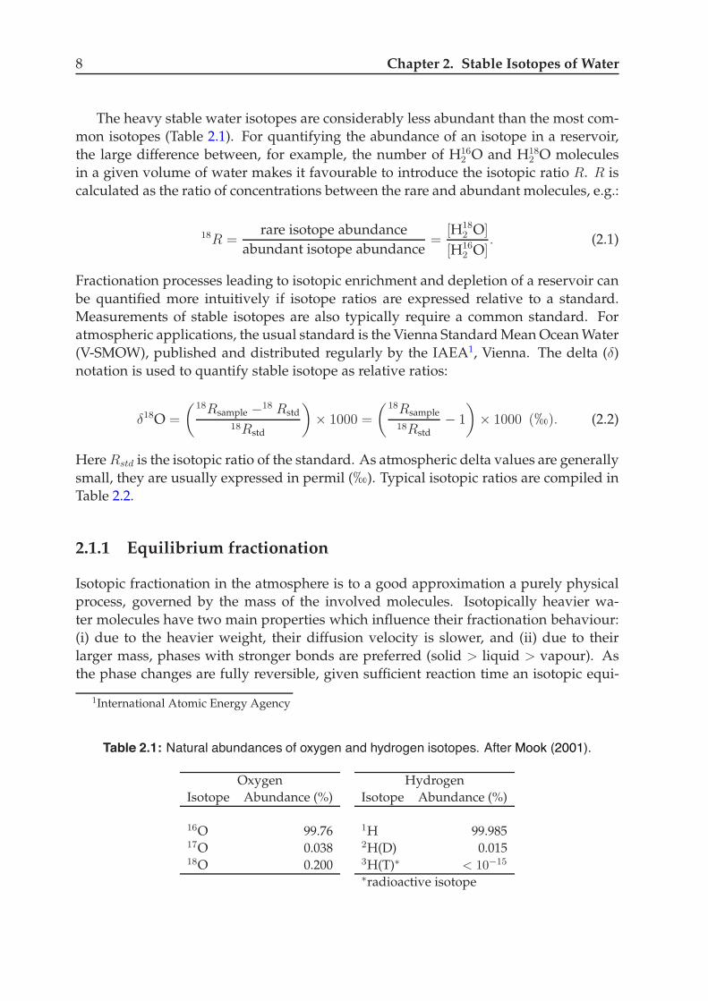
The heavy stable water isotopes are considerably less abundant than the most com-mon isotopes (Table 2.1). For quantifying the abundance of an isotope in a reservoir,the large difference between, for example, the number of H16
2 O and H182 O molecules
in a given volume of water makes it favourable to introduce the isotopic ratio R. R iscalculated as the ratio of concentrations between the rare and abundant molecules, e.g.:
18R =rare isotope abundance
abundant isotope abundance=
[H182 O]
[H162 O]
. (2.1)
Fractionation processes leading to isotopic enrichment and depletion of a reservoir canbe quantified more intuitively if isotope ratios are expressed relative to a standard.Measurements of stable isotopes are also typically require a common standard. Foratmospheric applications, the usual standard is the Vienna Standard Mean Ocean Water(V-SMOW), published and distributed regularly by the IAEA1, Vienna. The delta (!)notation is used to quantify stable isotope as relative ratios:
!18O =
!18Rsample !18 Rstd
18Rstd
"
" 1000 =
!18Rsample
18Rstd! 1
"
" 1000 (!). (2.2)
Here Rstd is the isotopic ratio of the standard. As atmospheric delta values are generallysmall, they are usually expressed in permil (!). Typical isotopic ratios are compiled inTable 2.2.
2.1.1 Equilibrium fractionation
Isotopic fractionation in the atmosphere is to a good approximation a purely physicalprocess, governed by the mass of the involved molecules. Isotopically heavier wa-ter molecules have two main properties which influence their fractionation behaviour:(i) due to the heavier weight, their diffusion velocity is slower, and (ii) due to theirlarger mass, phases with stronger bonds are preferred (solid > liquid > vapour). Asthe phase changes are fully reversible, given sufficient reaction time an isotopic equi-
1International Atomic Energy Agency
Table 2.1: Natural abundances of oxygen and hydrogen isotopes. After Mook (2001).
Oxygen HydrogenIsotope Abundance (%) Isotope Abundance (%)
16O 99.76 1H 99.98517O 0.038 2H(D) 0.01518O 0.200 3H(T)! < 10"15
!radioactive isotope
2.1. Background and definitions 9
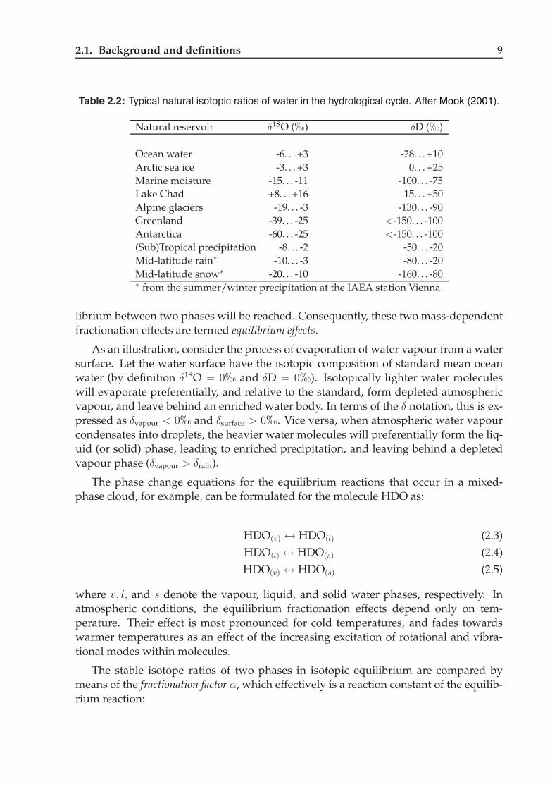
Table 2.2: Typical natural isotopic ratios of water in the hydrological cycle. After Mook (2001).
Natural reservoir !18O (!) !D (!)
Ocean water -6. . . +3 -28. . . +10Arctic sea ice -3. . . +3 0. . . +25Marine moisture -15. . . -11 -100. . . -75Lake Chad +8. . . +16 15. . . +50Alpine glaciers -19. . . -3 -130. . . -90Greenland -39. . . -25 <-150. . . -100Antarctica -60. . . -25 <-150. . . -100(Sub)Tropical precipitation -8. . . -2 -50. . . -20Mid-latitude rain! -10. . . -3 -80. . . -20Mid-latitude snow! -20. . . -10 -160. . . -80! from the summer/winter precipitation at the IAEA station Vienna.
librium between two phases will be reached. Consequently, these two mass-dependentfractionation effects are termed equilibrium effects.
As an illustration, consider the process of evaporation of water vapour from a watersurface. Let the water surface have the isotopic composition of standard mean oceanwater (by definition !18O = 0! and !D = 0!). Isotopically lighter water moleculeswill evaporate preferentially, and relative to the standard, form depleted atmosphericvapour, and leave behind an enriched water body. In terms of the ! notation, this is ex-pressed as !vapour < 0! and !surface > 0!. Vice versa, when atmospheric water vapourcondensates into droplets, the heavier water molecules will preferentially form the liq-uid (or solid) phase, leading to enriched precipitation, and leaving behind a depletedvapour phase (!vapour > !rain).
The phase change equations for the equilibrium reactions that occur in a mixed-phase cloud, for example, can be formulated for the molecule HDO as:
HDO(v) ! HDO(l) (2.3)
HDO(l) ! HDO(s) (2.4)
HDO(v) ! HDO(s) (2.5)
where v, l, and s denote the vapour, liquid, and solid water phases, respectively. Inatmospheric conditions, the equilibrium fractionation effects depend only on tem-perature. Their effect is most pronounced for cold temperatures, and fades towardswarmer temperatures as an effect of the increasing excitation of rotational and vibra-tional modes within molecules.
The stable isotope ratios of two phases in isotopic equilibrium are compared bymeans of the fractionation factor ", which effectively is a reaction constant of the equilib-rium reaction:
10 Chapter 2. Stable Isotopes of Water
!v/l =18Rv
18Rl=
"18v O + 1000
"18l O + 1000
(2.6)
Typically, ! is very close to 1.0, which is why frequently fractionation is expressed eitheras 1000 ! ln(!) or as #:
# = (! " 1) ! 1000. (2.7)
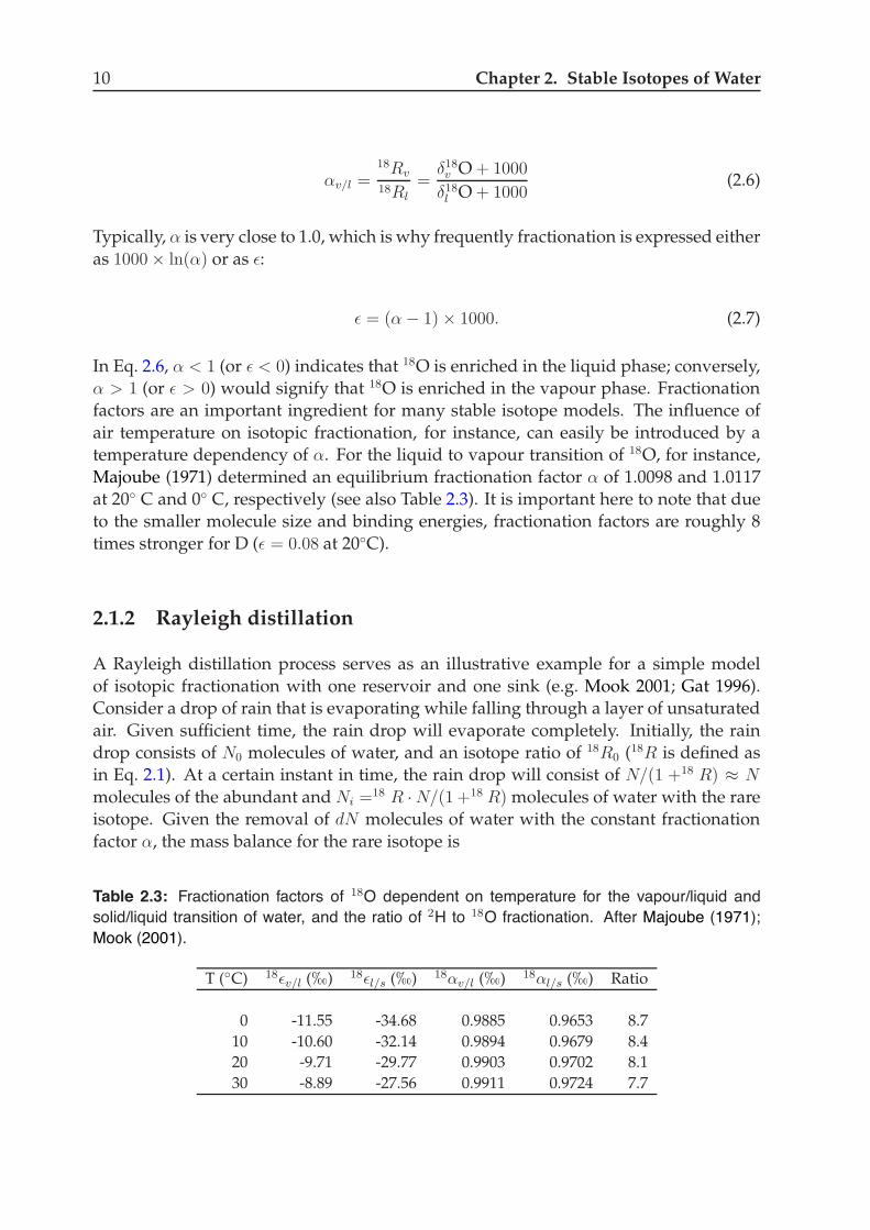
In Eq. 2.6, ! < 1 (or # < 0) indicates that 18O is enriched in the liquid phase; conversely,! > 1 (or # > 0) would signify that 18O is enriched in the vapour phase. Fractionationfactors are an important ingredient for many stable isotope models. The influence ofair temperature on isotopic fractionation, for instance, can easily be introduced by atemperature dependency of !. For the liquid to vapour transition of 18O, for instance,Majoube (1971) determined an equilibrium fractionation factor ! of 1.0098 and 1.0117at 20! C and 0! C, respectively (see also Table 2.3). It is important here to note that dueto the smaller molecule size and binding energies, fractionation factors are roughly 8times stronger for D (# = 0.08 at 20!C).
2.1.2 Rayleigh distillation
A Rayleigh distillation process serves as an illustrative example for a simple modelof isotopic fractionation with one reservoir and one sink (e.g. Mook 2001; Gat 1996).Consider a drop of rain that is evaporating while falling through a layer of unsaturatedair. Given sufficient time, the rain drop will evaporate completely. Initially, the raindrop consists of N0 molecules of water, and an isotope ratio of 18R0 (18R is defined asin Eq. 2.1). At a certain instant in time, the rain drop will consist of N/(1 +18 R) # Nmolecules of the abundant and Ni =18 R ·N/(1 +18 R) molecules of water with the rareisotope. Given the removal of dN molecules of water with the constant fractionationfactor !, the mass balance for the rare isotope is
Table 2.3: Fractionation factors of 18O dependent on temperature for the vapour/liquid andsolid/liquid transition of water, and the ratio of 2H to 18O fractionation. After Majoube (1971);Mook (2001).
T (!C) 18!v/l (!) 18!l/s (!) 18"v/l (!) 18"l/s (!) Ratio
0 -11.55 -34.68 0.9885 0.9653 8.710 -10.60 -32.14 0.9894 0.9679 8.420 -9.71 -29.77 0.9903 0.9702 8.130 -8.89 -27.56 0.9911 0.9724 7.7
2.1. Background and definitions 11
18R
1 +18 RN =
18R + d18R
1 +18 R + d18R(N + dN) !
!18R
1 + !18RdN. (2.8)
Taking all denominators equal to 18R + 1 and neglecting products of differentials, thisequation becomes
d18R18R
=dN
N(! ! 1). (2.9)
With the initial conditions N0 and 18R0, Eq. 2.9 can be integrated to
18R =18 R0
!
N
N0
"!!1
=18 R0 · f!!1 (2.10)
or, in " notation
"18O =1 + "18
0 O
f "! 1. (2.11)
Here, f = N/N0 is the fraction of the reservoir (the rain drop) which is remaining
surrounding vapourinstantaneousevaporateresidual reservoir
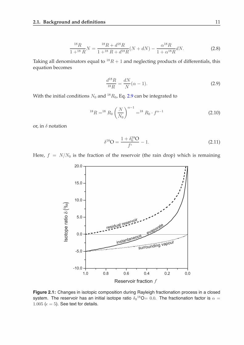
Figure 2.1: Changes in isotopic composition during Rayleigh fractionation process in a closedsystem. The reservoir has an initial isotope ratio !0
18O= 0.0. The fractionation factor is " =
1.005 (# = 5). See text for details.
12 Chapter 2. Stable Isotopes of Water
during the Rayleigh distillation. Fig. 2.1 shows the temporal evolution of the isotopiccomposition of the rain drop and the ambient water vapour, taking the reservoir frac-tion f as a (non-proportional) axis of time. The rain drop has an initial isotope ratio!0
18O= 0.0, and " = 1.005 (or # = 5). The residual rain drop has an increasingly en-riched isotopic composition during the fractionation process (Fig. 2.1, dashed line), asthe light isotopes evaporate preferentially. The isotopic ratio of the instantaneous evap-orate (Fig. 2.1, solid line) however also depends on the isotopic composition of thereservoir, and hence becomes increasingly enriched during the distillation. Note thatthe isotopic offset (Fig.2.1, arrow) according to the fractionation factor is constant withf . The isotopic composition of the total surrounding vapour (Fig. 2.1, dotted line) ac-cordingly increases from the smallest value !18O= !5! for f = 1 to zero (the initialcomposition of the liquid phase) at f = 0, i.e. when the rain drop has completely evap-orated.
Rayleigh distillation models are widely applied in isotope studies in the atmo-spheric sciences (see Section 2.6), and can be further extended by considering severalcoupled reservoirs, and modified to describe open systems systems (Gat 1996; Mook2001).
2.1.3 Non-equilibrium (kinetic) fractionation
In addition to the equilibrium fractionation effects, so-called kinetic or non-equilibriumfractionation can take place during phase changes. If the evaporating water vapourabove a water surface is for example continuously transported away by turbulent pro-cesses, the phase change reaction cannot reach an equilibrium, i.e. it is forced towardsone side of the reaction equation, e.g.
HDO(l) " HDO(v). (2.12)
In the transition from the saturated water surface to the turbulent boundary layer, watervapour passes through an intermediate layer where molecular diffusion velocities areimportant. Diffusion velocities are different for the two water isotope molecules HDOand H18
2 O. Unlike in equilibrium fractionation, there is not enough time, mostly for theslower-moving H18
2 O molecules, to reach an equilibrium state, which results in mea-surable deviations from equilibrium conditions. Namely, the fractionation ratio of thetwo molecules will deviate from the #1:8 ratio observed under equilibrium conditions(Table 2.3). The effects of non-equilibrium fractionation is quantified as the Deuteriumexcess (d-excess) (Dansgaard 1964). The d-excess is defined by the deviation of the com-bined isotopic information of !D and !18O from the relative fractionation under normalconditions:
d = !D ! 8 · !18O (!). (2.13)
2.2. Isotope fractionation processes 13
The extent of non-equilibrium fractionation during evaporation is influenced by vari-ous factors, such as the relative humidity gradient above the water surface, air and wa-ter temperature, and the evaporative cooling of the water surface (Merlivat and Jouzel1979; Cappa et al. 2003).
Some controversy surrounds the interpretation of this secondary isotope parame-ter. While usually being interpreted as a signal of the evaporation conditions, often inparticular as sea surface temperature signal (Barlow et al. 1993; Delaygue et al. 2000),kinetic fractionation does also occur during other atmospheric processes, e.g. in mixed-phase clouds during ice supersaturation (Ciais and Jouzel 1994; Ciais et al. 1995, seebelow).
Now that the basic notions of stable isotope processes have been laid out, a detailedand quantitative review of fractionation processes is undertaken in the following sec-tion.
2.2 Isotope fractionation processes
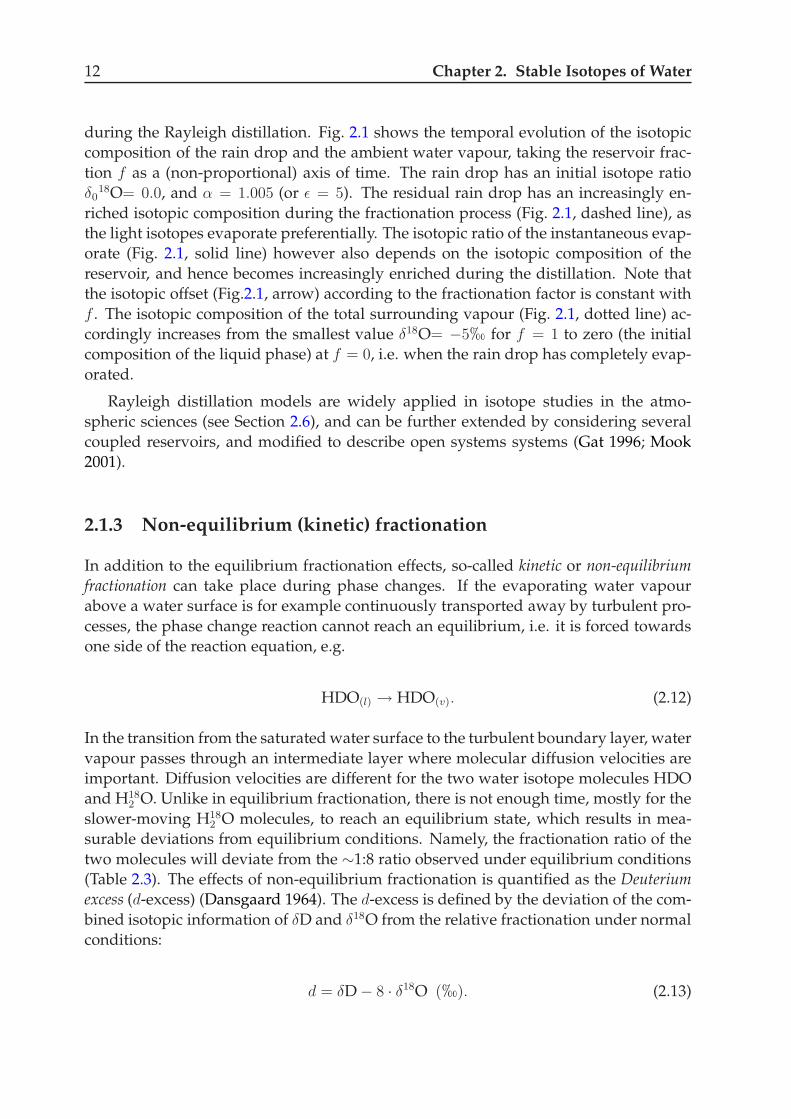
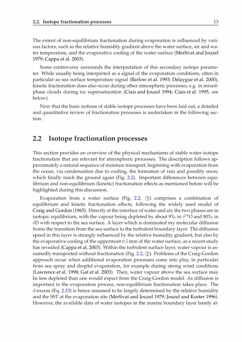
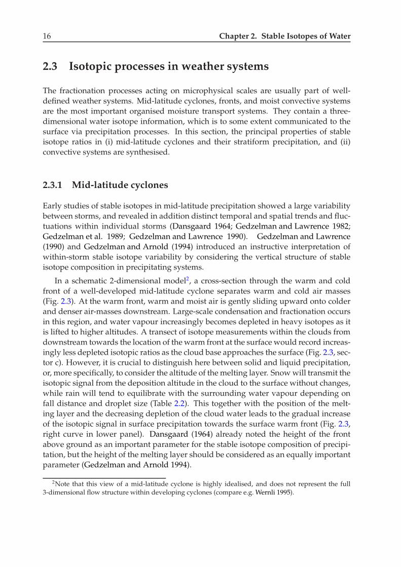
This section provides an overview of the physical mechanisms of stable water isotopefractionation that are relevant for atmospheric processes. The description follows ap-proximately a natural sequence of moisture transport, beginning with evaporation fromthe ocean, via condensation due to cooling, the formation of rain and possibly snow,which finally reach the ground again (Fig. 2.2). Important differences between equi-librium and non-equilibrium (kinetic) fractionation effects as mentioned before will behighlighted during this discussion.
Evaporation from a water surface (Fig. 2.2, !1 ) comprises a combination ofequilibrium and kinetic fractionation effects, following the widely used model ofCraig and Gordon (1965). Directly at the interface of water and air, the two phases are inisotopic equilibrium, with the vapour being depleted by about 9! in !18O and 80! in!D with respect to the sea surface. A layer which is dominated my molecular diffusionfroms the transition from the sea surface to the turbulent boundary layer. The diffusionspeed in this layer is strongly influenced by the relative humidity gradient, but also bythe evaporative cooling of the uppermost 0.5 mm of the water surface, as a recent studyhas revealed (Cappa et al. 2003). Within the turbulent surface layer, water vapour is as-sumedly transported without fractionation (Fig. 2.2, !2 ). Problems of the Craig-Gordonapproach occur when additional evaporation processes come into play, in particularfrom sea spray and droplet evaporation, for example during strong wind conditions(Lawrence et al. 1998; Gat et al. 2003). Then, water vapour above the sea surface maybe less depleted than one would expect from the Craig-Gordon model. As diffusion isimportant in the evaporation process, non-equilibrium fractionation takes place. Thed-excess (Eq. 2.13) is hence assumed to be largely determined by the relative humidityand the SST at the evaporation site (Merlivat and Jouzel 1979; Jouzel and Koster 1996).However, the available data of water isotopes in the marine boundary layer barely al-
14 Chapter 2. Stable Isotopes of Water
1
2
3
4
5
6
7
8
melting
layer
RH
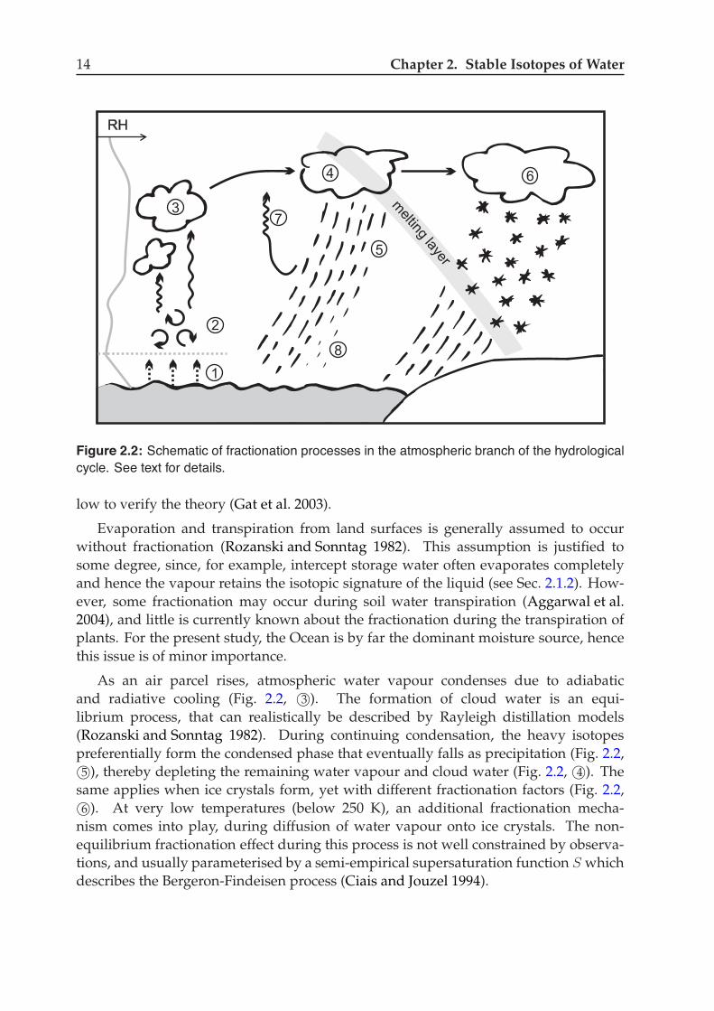
Figure 2.2: Schematic of fractionation processes in the atmospheric branch of the hydrologicalcycle. See text for details.
low to verify the theory (Gat et al. 2003).
Evaporation and transpiration from land surfaces is generally assumed to occurwithout fractionation (Rozanski and Sonntag 1982). This assumption is justified tosome degree, since, for example, intercept storage water often evaporates completelyand hence the vapour retains the isotopic signature of the liquid (see Sec. 2.1.2). How-ever, some fractionation may occur during soil water transpiration (Aggarwal et al.2004), and little is currently known about the fractionation during the transpiration ofplants. For the present study, the Ocean is by far the dominant moisture source, hencethis issue is of minor importance.
As an air parcel rises, atmospheric water vapour condenses due to adiabaticand radiative cooling (Fig. 2.2, !3 ). The formation of cloud water is an equi-librium process, that can realistically be described by Rayleigh distillation models(Rozanski and Sonntag 1982). During continuing condensation, the heavy isotopespreferentially form the condensed phase that eventually falls as precipitation (Fig. 2.2,!5 ), thereby depleting the remaining water vapour and cloud water (Fig. 2.2, !4 ). Thesame applies when ice crystals form, yet with different fractionation factors (Fig. 2.2,!6 ). At very low temperatures (below 250 K), an additional fractionation mecha-nism comes into play, during diffusion of water vapour onto ice crystals. The non-equilibrium fractionation effect during this process is not well constrained by observa-tions, and usually parameterised by a semi-empirical supersaturation function S whichdescribes the Bergeron-Findeisen process (Ciais and Jouzel 1994).
2.2. Isotope fractionation processes 15
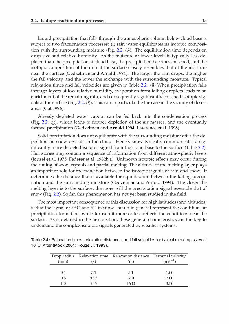
Liquid precipitation that falls through the atmospheric column below cloud base issubject to two fractionation processes: (i) rain water equilibrates its isotopic composi-tion with the surrounding moisture (Fig. 2.2, !5 ). The equilibration time depends ondrop size and relative humidity. As the moisture at lower levels is typically less de-pleted than the precipitation at cloud base, the precipitation becomes enriched, and theisotopic composition of the rain at the surface closely resembles that of the moisturenear the surface (Gedzelman and Arnold 1994). The larger the rain drops, the higherthe fall velocity, and the lower the exchange with the surrounding moisture. Typicalrelaxation times and fall velocities are given in Table 2.2. (ii) When precipitation fallsthrough layers of low relative humidity, evaporation from falling droplets leads to anenrichment of the remaining rain, and consequently significantly enriched isotopic sig-nals at the surface (Fig. 2.2, !8 ). This can in particular be the case in the vicinity of desertareas (Gat 1996).
Already depleted water vapour can be fed back into the condensation process(Fig. 2.2, !7 ), which leads to further depletion of the air masses, and the eventuallyformed precipitation (Gedzelman and Arnold 1994; Lawrence et al. 1998).
Solid precipitation does not equilibrate with the surrounding moisture after the de-position on snow crystals in the cloud. Hence, snow typically communicates a sig-nificantly more depleted isotopic signal from the cloud base to the surface (Table 2.2).Hail stones may contain a sequence of information from different atmospheric levels(Jouzel et al. 1975; Federer et al. 1982b,a). Unknown isotopic effects may occur duringthe riming of snow crystals and partial melting. The altitude of the melting layer playsan important role for the transition between the isotopic signals of rain and snow. Itdetermines the distance that is available for equilibration between the falling precip-itation and the surrounding moisture (Gedzelman and Arnold 1994). The closer themelting layer is to the surface, the more will the precipitation signal resemble that ofsnow (Fig. 2.2). So far, this phenomenon has not yet been studied in the field.
The most important consequence of this discussion for high latitudes (and altitudes)is that the signal of !18O and !D in snow should in general represent the conditions atprecipitation formation, while for rain it more or less reflects the conditions near thesurface. As is detailed in the next section, these general characteristics are the key tounderstand the complex isotopic signals generated by weather systems.
Table 2.4: Relaxation times, relaxation distances, and fall velocities for typical rain drop sizes at10!C. After (Mook 2001; Houze Jr. 1993).
Drop radius Relaxation time Relaxation distance Terminal velocity(mm) (s) (m) (ms"1)
0.1 7.1 5.1 1.000.5 92.5 370 2.001.0 246 1600 3.50
16 Chapter 2. Stable Isotopes of Water
2.3 Isotopic processes in weather systems
The fractionation processes acting on microphysical scales are usually part of well-defined weather systems. Mid-latitude cyclones, fronts, and moist convective systemsare the most important organised moisture transport systems. They contain a three-dimensional water isotope information, which is to some extent communicated to thesurface via precipitation processes. In this section, the principal properties of stableisotope ratios in (i) mid-latitude cyclones and their stratiform precipitation, and (ii)convective systems are synthesised.
2.3.1 Mid-latitude cyclones
Early studies of stable isotopes in mid-latitude precipitation showed a large variabilitybetween storms, and revealed in addition distinct temporal and spatial trends and fluc-tuations within individual storms (Dansgaard 1964; Gedzelman and Lawrence 1982;Gedzelman et al. 1989; Gedzelman and Lawrence 1990). Gedzelman and Lawrence(1990) and Gedzelman and Arnold (1994) introduced an instructive interpretation ofwithin-storm stable isotope variability by considering the vertical structure of stableisotope composition in precipitating systems.
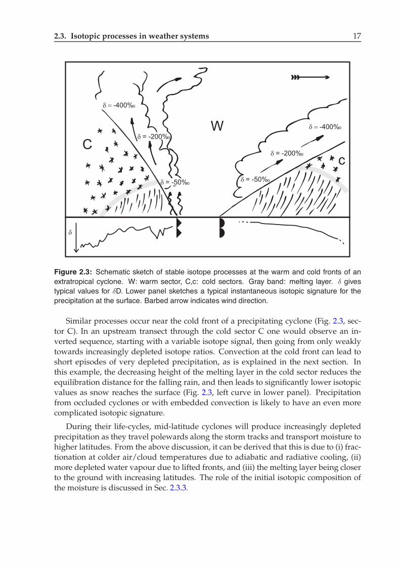
In a schematic 2-dimensional model2, a cross-section through the warm and coldfront of a well-developed mid-latitude cyclone separates warm and cold air masses(Fig. 2.3). At the warm front, warm and moist air is gently sliding upward onto colderand denser air-masses downstream. Large-scale condensation and fractionation occursin this region, and water vapour increasingly becomes depleted in heavy isotopes as itis lifted to higher altitudes. A transect of isotope measurements within the clouds fromdownstream towards the location of the warm front at the surface would record increas-ingly less depleted isotopic ratios as the cloud base approaches the surface (Fig. 2.3, sec-tor c). However, it is crucial to distinguish here between solid and liquid precipitation,or, more specifically, to consider the altitude of the melting layer. Snow will transmit theisotopic signal from the deposition altitude in the cloud to the surface without changes,while rain will tend to equilibrate with the surrounding water vapour depending onfall distance and droplet size (Table 2.2). This together with the position of the melt-ing layer and the decreasing depletion of the cloud water leads to the gradual increaseof the isotopic signal in surface precipitation towards the surface warm front (Fig. 2.3,right curve in lower panel). Dansgaard (1964) already noted the height of the frontabove ground as an important parameter for the stable isotope composition of precipi-tation, but the height of the melting layer should be considered as an equally importantparameter (Gedzelman and Arnold 1994).
2Note that this view of a mid-latitude cyclone is highly idealised, and does not represent the full3-dimensional flow structure within developing cyclones (compare e.g. Wernli 1995).
2.3. Isotopic processes in weather systems 17
!
C
W
c! = -50%0
! = -200%0
!"# -400%0
!"# -400%0
! = -200%0
! = -50%0
Figure 2.3: Schematic sketch of stable isotope processes at the warm and cold fronts of anextratropical cyclone. W: warm sector, C,c: cold sectors. Gray band: melting layer. ! givestypical values for !D. Lower panel sketches a typical instantaneous isotopic signature for theprecipitation at the surface. Barbed arrow indicates wind direction.
Similar processes occur near the cold front of a precipitating cyclone (Fig. 2.3, sec-tor C). In an upstream transect through the cold sector C one would observe an in-verted sequence, starting with a variable isotope signal, then going from only weaklytowards increasingly depleted isotope ratios. Convection at the cold front can lead toshort episodes of very depleted precipitation, as is explained in the next section. Inthis example, the decreasing height of the melting layer in the cold sector reduces theequilibration distance for the falling rain, and then leads to significantly lower isotopicvalues as snow reaches the surface (Fig. 2.3, left curve in lower panel). Precipitationfrom occluded cyclones or with embedded convection is likely to have an even morecomplicated isotopic signature.
During their life-cycles, mid-latitude cyclones will produce increasingly depletedprecipitation as they travel polewards along the storm tracks and transport moisture tohigher latitudes. From the above discussion, it can be derived that this is due to (i) frac-tionation at colder air/cloud temperatures due to adiabatic and radiative cooling, (ii)more depleted water vapour due to lifted fronts, and (iii) the melting layer being closerto the ground with increasing latitudes. The role of the initial isotopic composition ofthe moisture is discussed in Sec. 2.3.3.
18 Chapter 2. Stable Isotopes of Water
2.3.2 Convective systems
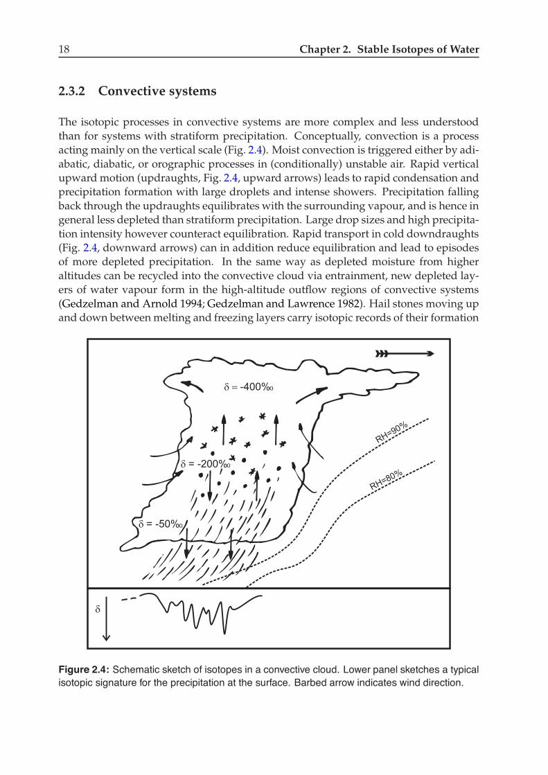
The isotopic processes in convective systems are more complex and less understoodthan for systems with stratiform precipitation. Conceptually, convection is a processacting mainly on the vertical scale (Fig. 2.4). Moist convection is triggered either by adi-abatic, diabatic, or orographic processes in (conditionally) unstable air. Rapid verticalupward motion (updraughts, Fig. 2.4, upward arrows) leads to rapid condensation andprecipitation formation with large droplets and intense showers. Precipitation fallingback through the updraughts equilibrates with the surrounding vapour, and is hence ingeneral less depleted than stratiform precipitation. Large drop sizes and high precipita-tion intensity however counteract equilibration. Rapid transport in cold downdraughts(Fig. 2.4, downward arrows) can in addition reduce equilibration and lead to episodesof more depleted precipitation. In the same way as depleted moisture from higheraltitudes can be recycled into the convective cloud via entrainment, new depleted lay-ers of water vapour form in the high-altitude outflow regions of convective systems(Gedzelman and Arnold 1994; Gedzelman and Lawrence 1982). Hail stones moving upand down between melting and freezing layers carry isotopic records of their formation
RH=90%
RH=80%
!
! = -50%0
! = -200%0
!"# -400%0
Figure 2.4: Schematic sketch of isotopes in a convective cloud. Lower panel sketches a typicalisotopic signature for the precipitation at the surface. Barbed arrow indicates wind direction.

2.3. Isotopic processes in weather systems 19
conditions to the surface (Federer et al. 1982b). If the convective cell precipitates intounsaturated air masses, rain water evaporation may again increase the isotope ratiosof the remaining rain. In an upstream transect below the convective cloud (Fig. 2.4,lower panel), an observer would generally measure a very variable isotopic signal, atfirst with slightly enriched isotope ratios, then strong excursions towards highly de-pleted values in downdraught and intense precipitation regions, and finally again aless depleted tailing-out of the isotope record, as equilibration in lighter rainfall sets inagain.
In the inter-tropical convergence zone (ITCZ), large-scale convective systems areresponsible for by far the largest part of the precipitation. In these areas, the isotopecharacteristics of convective systems also dominate the stable isotope seasonality inprecipitation. The moisture transport characteristics of Monsoon systems are at presentnot well understood. Again, such systems lead to sustained heavy precipitation withlarge droplets and relative humidity close to saturation below the cloud, which can al-low for the communication of depleted isotopic signals from high altitudes to groundlevel (see amount effect, pg. 24). In large-scale basins, such as the Amazon or centralChina, an important fraction of precipitation is recycled from land sources, which inaddition leads to successively depleted isotopes (see continentality effect, pg. 24). Trop-ical cyclonic systems, such as hurricanes, have been observed to produce very depletedprecipitation (Lawrence and Gedzelman 1996). Besides the very effective precipitationgeneration of such systems, which include embedded convective cells, moisture recy-cling between successive rain bands centered around the wall region has been proposedas a mechanism to produce such depleted isotopic signals (Lawrence et al. 1998).
2.3.3 Further remarks
In the above discussion, the initial isotopic composition of water vapour has not beentaken into consideration as a factor of influence. This influence is not well constrainedby observations, and is often assumed as equal to the isotopic ratios of precipitationnear the surface. The isotopic composition of !D and !18O near the surface can bemodelled, for example in a general circulation model (GCM) by means of the Craig-Gordon approach (see Sec. 2.6).
All of the above processes pose particular problems for the d-excess parameter, asvery little is known on non-equilibrium fractionation in clouds, and experimental datafrom the atmosphere are hardly available. While hence the short-term variability forthis parameter in precipitation or water vapour may be impossible to interpret, onlonger time scales it may still contain useful information, as will be further elucidatedbelow.
For a Lagrangian modelling approach the implications of the above discussion ofstable isotopes in weather systems are that after deposition in the cloud the isotopicratios of snow remain unchanged and should be successfully predictable by Rayleigh
20 Chapter 2. Stable Isotopes of Water
models. For rain, however, the processes acting below the cloud exert an importantinfluence on the isotopic ratios in precipitation at the surface, and should not be ne-glected. The preferred targets for Lagrangian isotope models are hence high latitudes,winter seasons, and high altitude locations.
In the following section, the understanding of the stable isotope signature of indi-vidual weather systems presented above will be applied to describe the mean globalwater isotope characteristics.
2.4 Isotopic processes on the seasonal to annual scale
On seasonal to annual time scales, a climatological mean state emerges from the super-position of weather-induced isotope signals. This isotopic mean state, in particular forprecipitation and the ocean surface, reflects some important characteristics of the globalhydrological cycle. Dansgaard’s (1964) work on the longer-term isotopic compositionin surface waters and precipitation was a corner stone to gain a semi-empirical under-standing of the atmospheric branch of the hydrological cycle. In this section, this now‘classical’ empirical view is re-interpreted from the viewpoint of a process-oriented un-derstanding of stable isotope fractionation. By regarding the so-called isotope effects intheir genetic context a physically consistent interpretation is achieved and conceptualcaveats become evident.
2.4.1 Annual mean isotopic signature
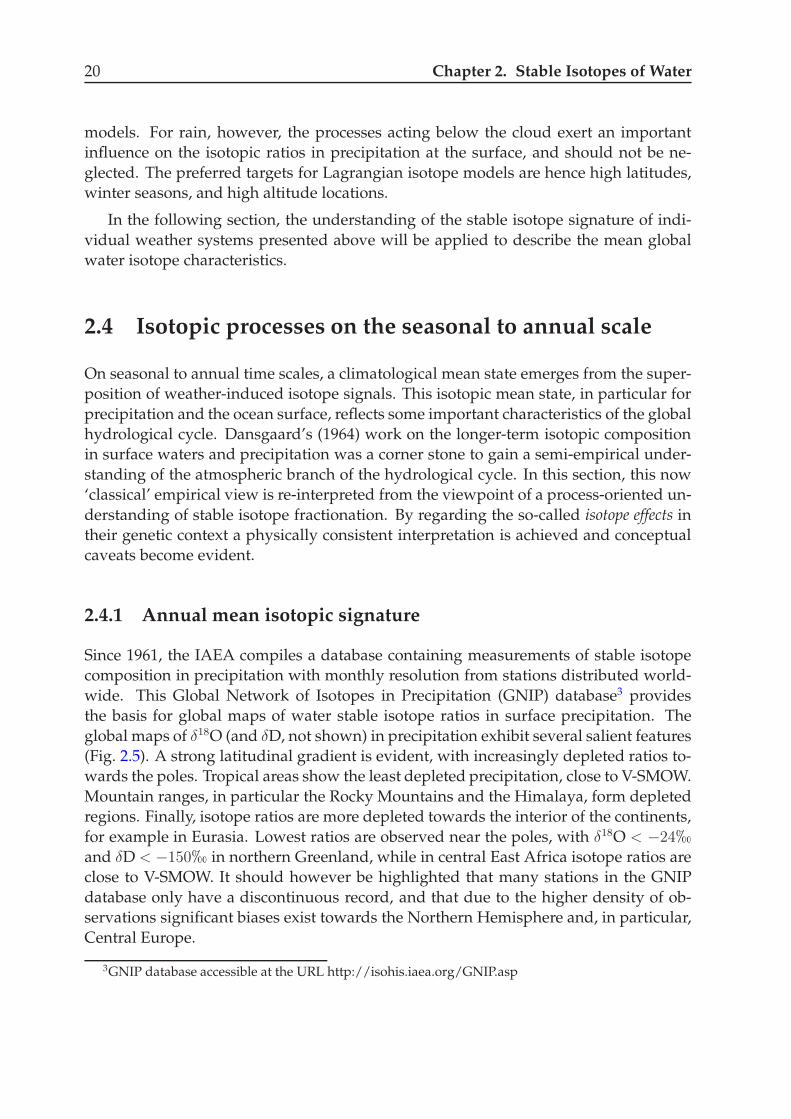
Since 1961, the IAEA compiles a database containing measurements of stable isotopecomposition in precipitation with monthly resolution from stations distributed world-wide. This Global Network of Isotopes in Precipitation (GNIP) database3 providesthe basis for global maps of water stable isotope ratios in surface precipitation. Theglobal maps of !18O (and !D, not shown) in precipitation exhibit several salient features(Fig. 2.5). A strong latitudinal gradient is evident, with increasingly depleted ratios to-wards the poles. Tropical areas show the least depleted precipitation, close to V-SMOW.Mountain ranges, in particular the Rocky Mountains and the Himalaya, form depletedregions. Finally, isotope ratios are more depleted towards the interior of the continents,for example in Eurasia. Lowest ratios are observed near the poles, with !18O < !24!and !D < !150! in northern Greenland, while in central East Africa isotope ratios areclose to V-SMOW. It should however be highlighted that many stations in the GNIPdatabase only have a discontinuous record, and that due to the higher density of ob-servations significant biases exist towards the Northern Hemisphere and, in particular,Central Europe.
3GNIP database accessible at the URL http://isohis.iaea.org/GNIP.asp
2.4. Isotopic processes on the seasonal to annual scale 21
Figure 2.5: Annual mean composition of !18O in precipitation compiled from the GNIP database(Araguas-Araguas et al. 2000)
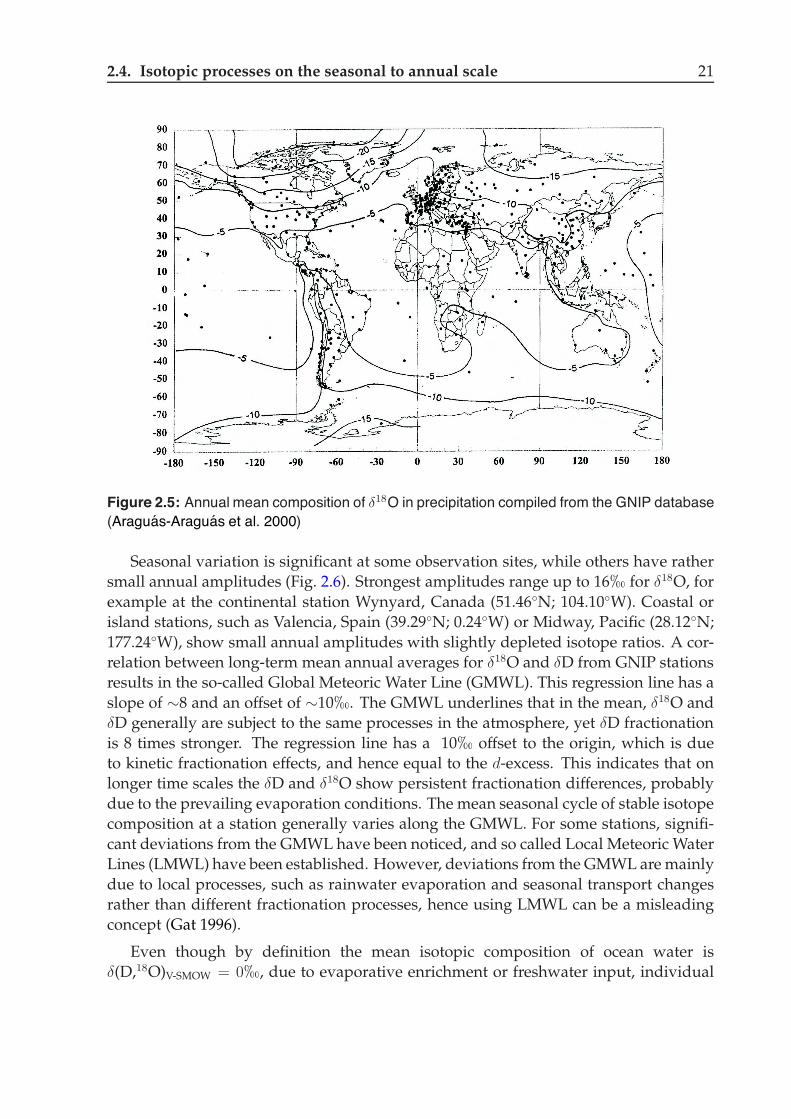
Seasonal variation is significant at some observation sites, while others have rathersmall annual amplitudes (Fig. 2.6). Strongest amplitudes range up to 16! for !18O, forexample at the continental station Wynyard, Canada (51.46!N; 104.10!W). Coastal orisland stations, such as Valencia, Spain (39.29!N; 0.24!W) or Midway, Pacific (28.12!N;177.24!W), show small annual amplitudes with slightly depleted isotope ratios. A cor-relation between long-term mean annual averages for !18O and !D from GNIP stationsresults in the so-called Global Meteoric Water Line (GMWL). This regression line has aslope of !8 and an offset of !10!. The GMWL underlines that in the mean, !18O and!D generally are subject to the same processes in the atmosphere, yet !D fractionationis 8 times stronger. The regression line has a 10! offset to the origin, which is dueto kinetic fractionation effects, and hence equal to the d-excess. This indicates that onlonger time scales the !D and !18O show persistent fractionation differences, probablydue to the prevailing evaporation conditions. The mean seasonal cycle of stable isotopecomposition at a station generally varies along the GMWL. For some stations, signifi-cant deviations from the GMWL have been noticed, and so called Local Meteoric WaterLines (LMWL) have been established. However, deviations from the GMWL are mainlydue to local processes, such as rainwater evaporation and seasonal transport changesrather than different fractionation processes, hence using LMWL can be a misleadingconcept (Gat 1996).
Even though by definition the mean isotopic composition of ocean water is!(D,18O)V-SMOW = 0!, due to evaporative enrichment or freshwater input, individual
22 Chapter 2. Stable Isotopes of Water
Figure 2.6: Selected seasonal cycles of !18O from Northern Hemisphere GNIP stations (Mook2001).
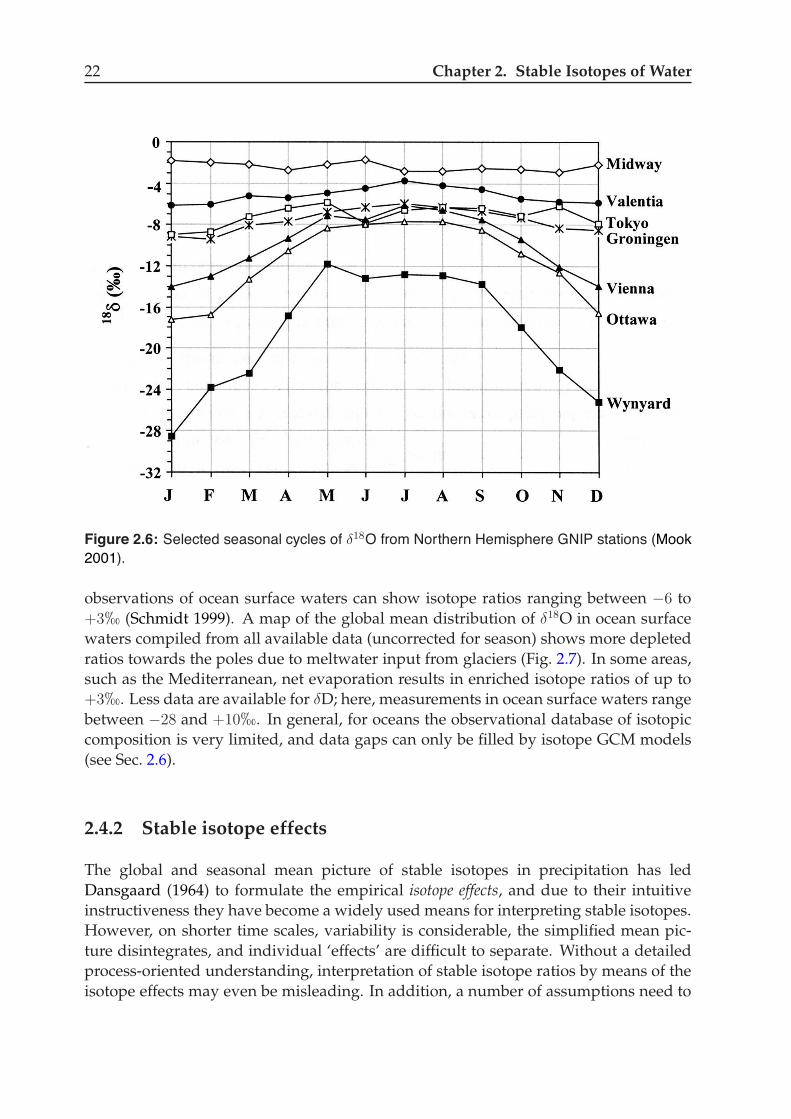
observations of ocean surface waters can show isotope ratios ranging between !6 to+3! (Schmidt 1999). A map of the global mean distribution of !18O in ocean surfacewaters compiled from all available data (uncorrected for season) shows more depletedratios towards the poles due to meltwater input from glaciers (Fig. 2.7). In some areas,such as the Mediterranean, net evaporation results in enriched isotope ratios of up to+3!. Less data are available for !D; here, measurements in ocean surface waters rangebetween !28 and +10!. In general, for oceans the observational database of isotopiccomposition is very limited, and data gaps can only be filled by isotope GCM models(see Sec. 2.6).
2.4.2 Stable isotope effects
The global and seasonal mean picture of stable isotopes in precipitation has ledDansgaard (1964) to formulate the empirical isotope effects, and due to their intuitiveinstructiveness they have become a widely used means for interpreting stable isotopes.However, on shorter time scales, variability is considerable, the simplified mean pic-ture disintegrates, and individual ‘effects’ are difficult to separate. Without a detailedprocess-oriented understanding, interpretation of stable isotope ratios by means of theisotope effects may even be misleading. In addition, a number of assumptions need to
2.4. Isotopic processes on the seasonal to annual scale 23
Figure 2.7: Ocean surface mean isotopic composition compiled from all available observations(Schmidt 1999).
be made, such as a fixed moisture source for global precipitation between 40! N and40! S, which now have partly been shown to be too simplified. Transport influencesare mostly neglected, even though they are very relevant for the interpretation of theglobal water isotope pattern (Rozanski et al. 1982).
In the following, Dansgaard’s isotope effects are listed and discussed from a process-oriented perspective.
Latitude effect: The latitude effect is based on the observation of a gradually depletedisotope signal in precipitation towards higher latitudes (Fig. 2.5). The averagegradient for !18O is !0.6!/! latitude in mid-latitudes, and up to !2!/! lati-tude in Antarctica (Mook 2001). Along with latitude, isotope ratios correlate withannual mean surface temperature according to the isotope-temperature relationship(!-T relationship) (Eq. 2.14, Dansgaard 1964):
!18O = 0.62 · T ! 15.25 (!). (2.14)
This relationship between stable isotopes and surface temperature has becomeone of the principal tools of paleoclimatology, primarily in the interpretation ofhigh-latitude ice cores. In light of the previous sections, it is evident that a num-ber of processes contribute to this latitude effect. Condensation temperature andhence fractionation factors change as moisture condensates at more northerly lat-itudes (Table 2.3). Precipitation increasingly falls as snow at high latitudes, and
24 Chapter 2. Stable Isotopes of Water
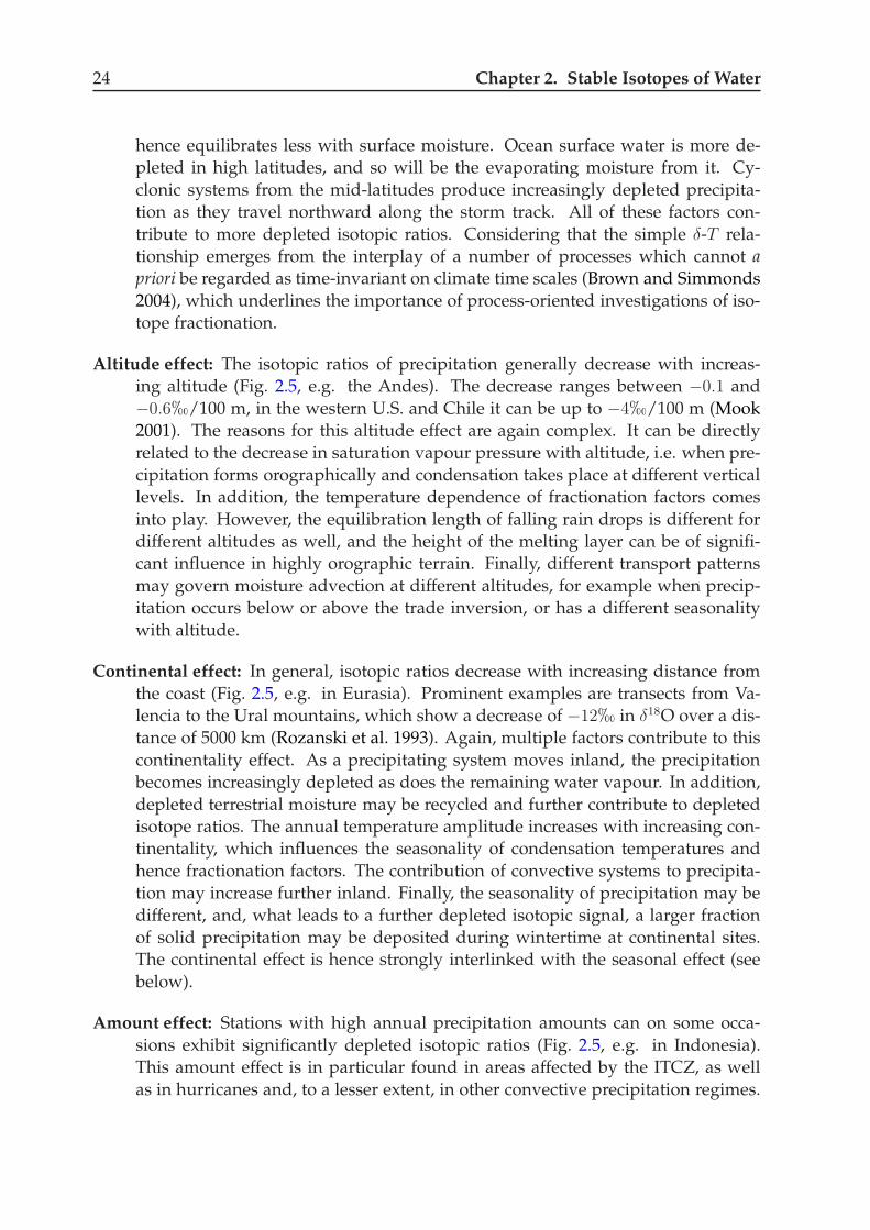
hence equilibrates less with surface moisture. Ocean surface water is more de-pleted in high latitudes, and so will be the evaporating moisture from it. Cy-clonic systems from the mid-latitudes produce increasingly depleted precipita-tion as they travel northward along the storm track. All of these factors con-tribute to more depleted isotopic ratios. Considering that the simple !-T rela-tionship emerges from the interplay of a number of processes which cannot apriori be regarded as time-invariant on climate time scales (Brown and Simmonds2004), which underlines the importance of process-oriented investigations of iso-tope fractionation.
Altitude effect: The isotopic ratios of precipitation generally decrease with increas-ing altitude (Fig. 2.5, e.g. the Andes). The decrease ranges between !0.1 and!0.6!/100 m, in the western U.S. and Chile it can be up to !4!/100 m (Mook2001). The reasons for this altitude effect are again complex. It can be directlyrelated to the decrease in saturation vapour pressure with altitude, i.e. when pre-cipitation forms orographically and condensation takes place at different verticallevels. In addition, the temperature dependence of fractionation factors comesinto play. However, the equilibration length of falling rain drops is different fordifferent altitudes as well, and the height of the melting layer can be of signifi-cant influence in highly orographic terrain. Finally, different transport patternsmay govern moisture advection at different altitudes, for example when precip-itation occurs below or above the trade inversion, or has a different seasonalitywith altitude.
Continental effect: In general, isotopic ratios decrease with increasing distance fromthe coast (Fig. 2.5, e.g. in Eurasia). Prominent examples are transects from Va-lencia to the Ural mountains, which show a decrease of !12! in !18O over a dis-tance of 5000 km (Rozanski et al. 1993). Again, multiple factors contribute to thiscontinentality effect. As a precipitating system moves inland, the precipitationbecomes increasingly depleted as does the remaining water vapour. In addition,depleted terrestrial moisture may be recycled and further contribute to depletedisotope ratios. The annual temperature amplitude increases with increasing con-tinentality, which influences the seasonality of condensation temperatures andhence fractionation factors. The contribution of convective systems to precipita-tion may increase further inland. Finally, the seasonality of precipitation may bedifferent, and, what leads to a further depleted isotopic signal, a larger fractionof solid precipitation may be deposited during wintertime at continental sites.The continental effect is hence strongly interlinked with the seasonal effect (seebelow).
Amount effect: Stations with high annual precipitation amounts can on some occa-sions exhibit significantly depleted isotopic ratios (Fig. 2.5, e.g. in Indonesia).This amount effect is in particular found in areas affected by the ITCZ, as wellas in hurricanes and, to a lesser extent, in other convective precipitation regimes.
2.5. Isotopic processes on the inter-annual to climate scale 25
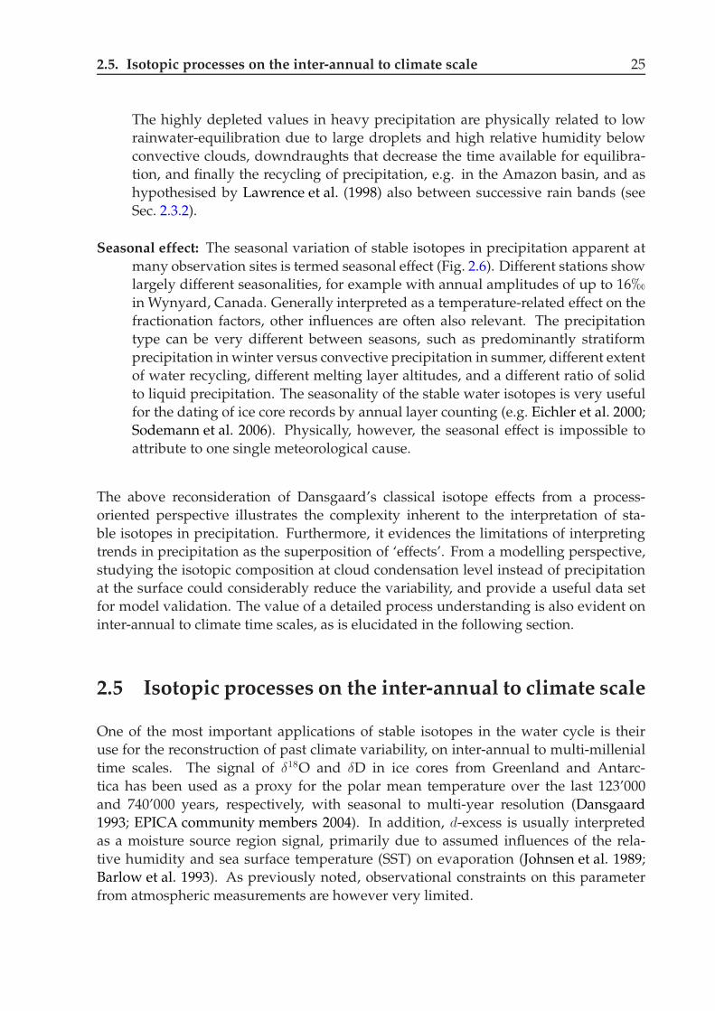
The highly depleted values in heavy precipitation are physically related to lowrainwater-equilibration due to large droplets and high relative humidity belowconvective clouds, downdraughts that decrease the time available for equilibra-tion, and finally the recycling of precipitation, e.g. in the Amazon basin, and ashypothesised by Lawrence et al. (1998) also between successive rain bands (seeSec. 2.3.2).
Seasonal effect: The seasonal variation of stable isotopes in precipitation apparent atmany observation sites is termed seasonal effect (Fig. 2.6). Different stations showlargely different seasonalities, for example with annual amplitudes of up to 16!
in Wynyard, Canada. Generally interpreted as a temperature-related effect on thefractionation factors, other influences are often also relevant. The precipitationtype can be very different between seasons, such as predominantly stratiformprecipitation in winter versus convective precipitation in summer, different extentof water recycling, different melting layer altitudes, and a different ratio of solidto liquid precipitation. The seasonality of the stable water isotopes is very usefulfor the dating of ice core records by annual layer counting (e.g. Eichler et al. 2000;Sodemann et al. 2006). Physically, however, the seasonal effect is impossible toattribute to one single meteorological cause.
The above reconsideration of Dansgaard’s classical isotope effects from a process-oriented perspective illustrates the complexity inherent to the interpretation of sta-ble isotopes in precipitation. Furthermore, it evidences the limitations of interpretingtrends in precipitation as the superposition of ‘effects’. From a modelling perspective,studying the isotopic composition at cloud condensation level instead of precipitationat the surface could considerably reduce the variability, and provide a useful data setfor model validation. The value of a detailed process understanding is also evident oninter-annual to climate time scales, as is elucidated in the following section.
2.5 Isotopic processes on the inter-annual to climate scale
One of the most important applications of stable isotopes in the water cycle is theiruse for the reconstruction of past climate variability, on inter-annual to multi-millenialtime scales. The signal of !18O and !D in ice cores from Greenland and Antarc-tica has been used as a proxy for the polar mean temperature over the last 123’000and 740’000 years, respectively, with seasonal to multi-year resolution (Dansgaard1993; EPICA community members 2004). In addition, d-excess is usually interpretedas a moisture source region signal, primarily due to assumed influences of the rela-tive humidity and sea surface temperature (SST) on evaporation (Johnsen et al. 1989;Barlow et al. 1993). As previously noted, observational constraints on this parameterfrom atmospheric measurements are however very limited.
26 Chapter 2. Stable Isotopes of Water
In the absence of detailed process-based knowledge, the primary tools for the pale-oclimatic interpretation of stable isotope records are the empirical isotope-temperaturerelationship, and the isotope effects proposed by Dansgaard (1964). However, consid-erable uncertainty exists on how constant this empirical relation has been through time,and on additional parameters that could influence this dependency (Jouzel et al. 1997;Brown and Simmonds 2004). Isotope GCM studies have more recently increased theunderstanding of isotope processes on climate time scales (see Sec. 2.6).
The main points of uncertainty are linked to the following questions:
(i) How do individual precipitation events translate into a mean value (Helsen et al.2005a)?
(ii) What is the relation between the surface and cloud temperatures?
(iii) What is the influence of transport variability?
(iv) Were the patterns and their seasonality of atmospheric moisture transport constanton climatic time scales (e.g., Krinner et al. 1997; Krinner and Werner 2003)?
(v) Which transformations can occur in the archive after deposition (e.g.,Delmotte et al. 2000)?
While questions (i)–(iii) are in the focus of the Lagrangian methodology introducedbelow, (iv) and (v) cannot be considered here.
Process-aimed studies are virtually impossible to accomplish on climate time scales,as direct observations are replaced by ever sparser proxy data from various archives asone goes further backward in time. One possibility to circumvent this difficulty is touse inter-annual variability of the present-day climate as a proxy for the atmosphericreorganisations that accompanied past climate variability. On inter-annual time scales,isotope data in precipitation during the last !50 years, mainly from firn cores, are as-sisted by reliable observations of the general circulation, such as reanalysis data.
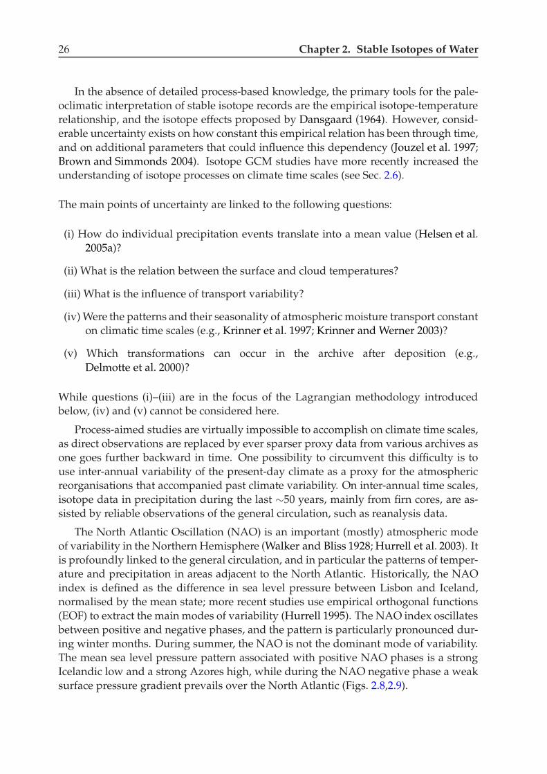
The North Atlantic Oscillation (NAO) is an important (mostly) atmospheric modeof variability in the Northern Hemisphere (Walker and Bliss 1928; Hurrell et al. 2003). Itis profoundly linked to the general circulation, and in particular the patterns of temper-ature and precipitation in areas adjacent to the North Atlantic. Historically, the NAOindex is defined as the difference in sea level pressure between Lisbon and Iceland,normalised by the mean state; more recent studies use empirical orthogonal functions(EOF) to extract the main modes of variability (Hurrell 1995). The NAO index oscillatesbetween positive and negative phases, and the pattern is particularly pronounced dur-ing winter months. During summer, the NAO is not the dominant mode of variability.The mean sea level pressure pattern associated with positive NAO phases is a strongIcelandic low and a strong Azores high, while during the NAO negative phase a weaksurface pressure gradient prevails over the North Atlantic (Figs. 2.8,2.9).
2.5. Isotopic processes on the inter-annual to climate scale 27
(a)
984
996
996
996
1008
1008
1008
10081020
1020
1020
1020
1020
1020
1020
1020
1020
1020
1020
1020
1020
(b)
1008
1008
1020
1020
1020
1020
10201020
10201020
1020
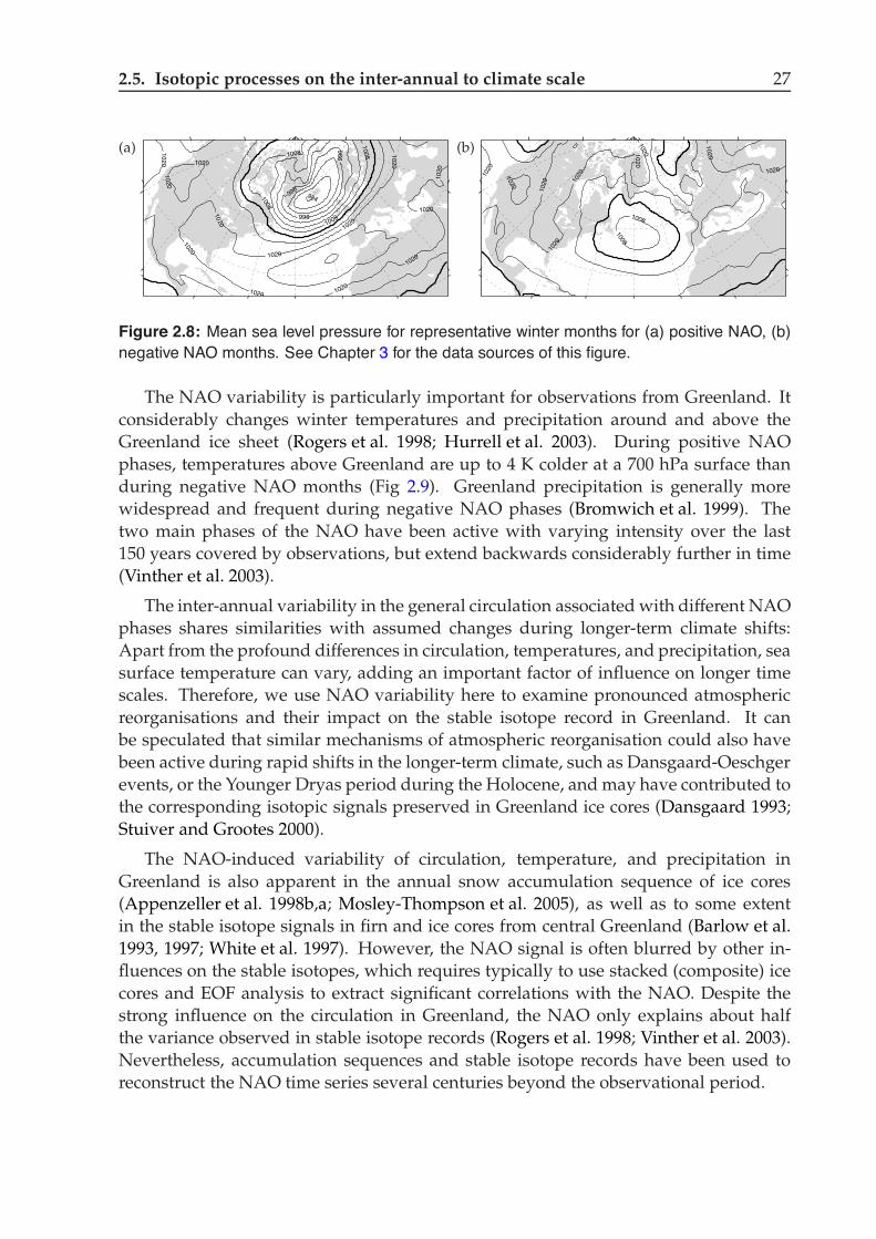
Figure 2.8: Mean sea level pressure for representative winter months for (a) positive NAO, (b)negative NAO months. See Chapter 3 for the data sources of this figure.
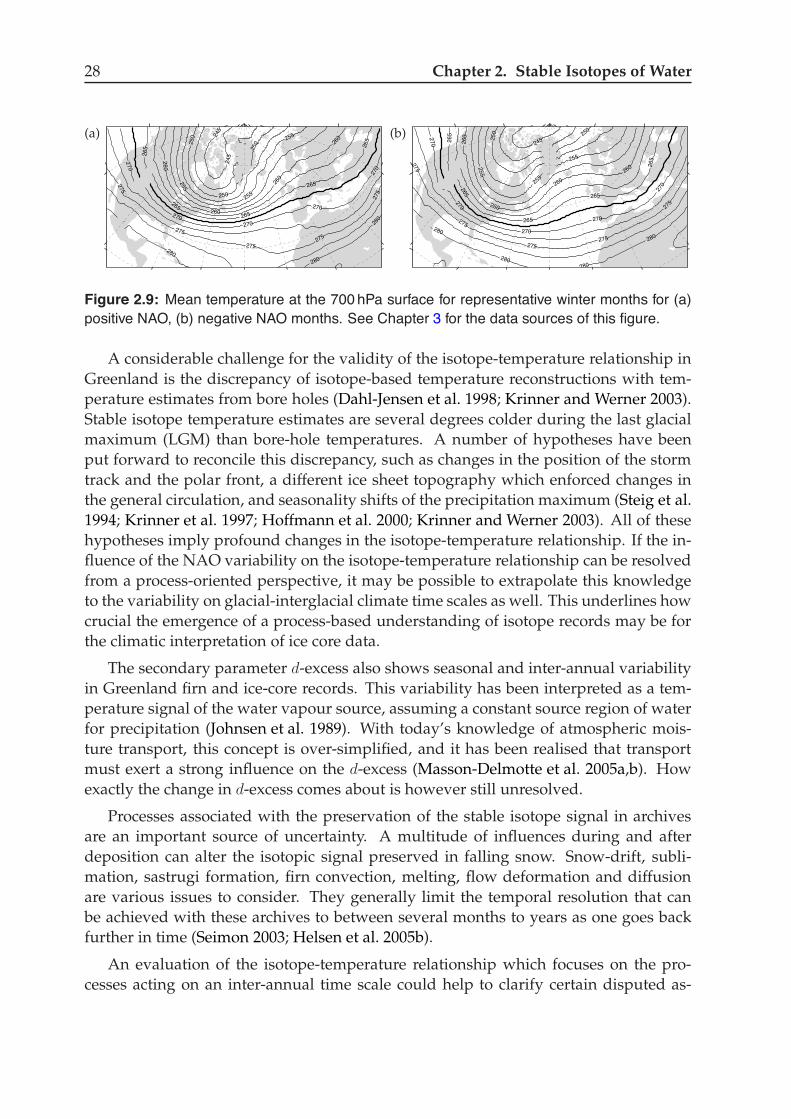
The NAO variability is particularly important for observations from Greenland. Itconsiderably changes winter temperatures and precipitation around and above theGreenland ice sheet (Rogers et al. 1998; Hurrell et al. 2003). During positive NAOphases, temperatures above Greenland are up to 4 K colder at a 700 hPa surface thanduring negative NAO months (Fig 2.9). Greenland precipitation is generally morewidespread and frequent during negative NAO phases (Bromwich et al. 1999). Thetwo main phases of the NAO have been active with varying intensity over the last150 years covered by observations, but extend backwards considerably further in time(Vinther et al. 2003).
The inter-annual variability in the general circulation associated with different NAOphases shares similarities with assumed changes during longer-term climate shifts:Apart from the profound differences in circulation, temperatures, and precipitation, seasurface temperature can vary, adding an important factor of influence on longer timescales. Therefore, we use NAO variability here to examine pronounced atmosphericreorganisations and their impact on the stable isotope record in Greenland. It canbe speculated that similar mechanisms of atmospheric reorganisation could also havebeen active during rapid shifts in the longer-term climate, such as Dansgaard-Oeschgerevents, or the Younger Dryas period during the Holocene, and may have contributed tothe corresponding isotopic signals preserved in Greenland ice cores (Dansgaard 1993;Stuiver and Grootes 2000).
The NAO-induced variability of circulation, temperature, and precipitation inGreenland is also apparent in the annual snow accumulation sequence of ice cores(Appenzeller et al. 1998b,a; Mosley-Thompson et al. 2005), as well as to some extentin the stable isotope signals in firn and ice cores from central Greenland (Barlow et al.1993, 1997; White et al. 1997). However, the NAO signal is often blurred by other in-fluences on the stable isotopes, which requires typically to use stacked (composite) icecores and EOF analysis to extract significant correlations with the NAO. Despite thestrong influence on the circulation in Greenland, the NAO only explains about halfthe variance observed in stable isotope records (Rogers et al. 1998; Vinther et al. 2003).Nevertheless, accumulation sequences and stable isotope records have been used toreconstruct the NAO time series several centuries beyond the observational period.
28 Chapter 2. Stable Isotopes of Water
(a) 245
245
250
250
250
255
255
255
260
260
260
260
265
265265
265
265
270
270270
270
270
275
275
275275
275
280280
280
(b)245
250 250
255
255
255
260
260
260260
265
265
265
265
265
270
270
270
270
270
275
275
275275
275
280
280280
280
Figure 2.9: Mean temperature at the 700hPa surface for representative winter months for (a)positive NAO, (b) negative NAO months. See Chapter 3 for the data sources of this figure.
A considerable challenge for the validity of the isotope-temperature relationship inGreenland is the discrepancy of isotope-based temperature reconstructions with tem-perature estimates from bore holes (Dahl-Jensen et al. 1998; Krinner and Werner 2003).Stable isotope temperature estimates are several degrees colder during the last glacialmaximum (LGM) than bore-hole temperatures. A number of hypotheses have beenput forward to reconcile this discrepancy, such as changes in the position of the stormtrack and the polar front, a different ice sheet topography which enforced changes inthe general circulation, and seasonality shifts of the precipitation maximum (Steig et al.1994; Krinner et al. 1997; Hoffmann et al. 2000; Krinner and Werner 2003). All of thesehypotheses imply profound changes in the isotope-temperature relationship. If the in-fluence of the NAO variability on the isotope-temperature relationship can be resolvedfrom a process-oriented perspective, it may be possible to extrapolate this knowledgeto the variability on glacial-interglacial climate time scales as well. This underlines howcrucial the emergence of a process-based understanding of isotope records may be forthe climatic interpretation of ice core data.
The secondary parameter d-excess also shows seasonal and inter-annual variabilityin Greenland firn and ice-core records. This variability has been interpreted as a tem-perature signal of the water vapour source, assuming a constant source region of waterfor precipitation (Johnsen et al. 1989). With today’s knowledge of atmospheric mois-ture transport, this concept is over-simplified, and it has been realised that transportmust exert a strong influence on the d-excess (Masson-Delmotte et al. 2005a,b). Howexactly the change in d-excess comes about is however still unresolved.
Processes associated with the preservation of the stable isotope signal in archivesare an important source of uncertainty. A multitude of influences during and afterdeposition can alter the isotopic signal preserved in falling snow. Snow-drift, subli-mation, sastrugi formation, firn convection, melting, flow deformation and diffusionare various issues to consider. They generally limit the temporal resolution that canbe achieved with these archives to between several months to years as one goes backfurther in time (Seimon 2003; Helsen et al. 2005b).
An evaluation of the isotope-temperature relationship which focuses on the pro-cesses acting on an inter-annual time scale could help to clarify certain disputed as-
2.6. Modelling of stable water isotopes 29
pects: What is the spatial variability of isotopic signals on the Greenland plateau?How strong is the event-to-event variability in isotopic parameters? Does the isotope-temperature relationship vary with changes in the NAO? Stable isotope models areinvaluable means to accomplish this task. Their past and present use, as well as a pro-posed extension are compiled in the following section.
2.6 Modelling of stable water isotopes
Aiming to enhance the understanding of stable water isotope processes on local toglobal scales, current stable isotope models attempt to synthesise the available knowl-edge on stable isotope processes to various degrees. From the earliest Rayleigh-distillation models, research has advanced to GCMs which have stable isotope pro-cesses coupled into the model’s hydrological cycle (Joussaume et al. 1984). The (zero-dimensional) Rayleigh model has been presented as an example in Section 2.1. In thissection, details of more advanced modelling attempts are given, together with a discus-sion of the limitations of each model type. Furthermore, it is discussed how they canbe combined to study unresolved aspects of stable water isotopes in the atmosphere.
A fundamental distinction in stable isotope modelling can be made between twomodel families, namely Lagrangian and Eulerian approaches. The Lagrangian categoryconsiders the fractionation of the moisture in an air parcel during its transport throughspace and time. Eulerian model approaches calculate isotopic fractionation based onfirst principles for the whole temporally and spatially discretised model domain. Bothapproaches are seconded by parameterisations of sub-grid scale processes. While inboth categories increasingly complex models have been developed, several intermedi-ate approaches have been proposed recently which try to combine the advantages ofthe two families. A description of the characteristics, strengths and weaknesses for thevarious existing approaches provides the framework for the approach applied in thiswork.
Lagrangian Rayleigh models: Lagrangian Rayleigh distillation models are commonlyused in conjunction with prescribed idealised or ’climatological’ pseudo-trajectories, which follow the hypothetical path of atmospheric moisture trans-port (Dansgaard 1964; Johnsen et al. 1989). Jouzel and Merlivat (1984) andCiais and Jouzel (1994) included microphysics parameterisations into such amodel (Mixed Cloud Isotope Model, MCIM), which allowed an application tocold polar regimes. The original idea of the MCIM model was to understandstable isotope fractionation on climate time scales, but in principle it can be ap-plied to shorter time scales as well. The intriguing intuitiveness of this conceptis alleviated by a number of difficulties. First, idealised trajectories of moisturetransport do generally fall short of representing the large variability of atmo-spheric moisture transport, as they assume a fixed water source in the tropics.Second, due to lack of better information at that time, several parameterisations
30 Chapter 2. Stable Isotopes of Water
based on semi-empirical knowledge are build into the model. This concerns therelation between surface and cloud temperature and the kinetic fractionation ef-fect in supersaturated ice clouds. Finally, the initial isotope ratios of air parcelsare not well-constrained, while being quite important for the final isotope ratio(Jouzel and Koster 1996). Further details on the MCIM model are given in Ap-pendix C.
2D column models: Two-dimensional column models have been developed mainly toincrease the understanding of tropospheric isotope fractionation in the vertical(Rozanski and Sonntag 1982; Gedzelman and Arnold 1994). These models havebeen applied to precipitation events on time scales of hours to days, and partlycontain advanced microphysics parameterisations, such as cloud ice, liquid, grau-pel, hail, and vapour species. The strength of these models is to increase the un-derstanding of the vertical processes in idealised situations as they capture allprocesses that influence the isotopic ratio of surface precipitation. Furthermore,they help to understand observed time series of isotopes in precipitation on timescales of minutes to hours. Major limitations are the difficulty to initialise suchmodels (e.g. from soundings), the sparsity of vertical stable isotope profiles in thetroposphere to compare with, and the exclusion of isotope advection and fraction-ation during surface evaporation.
2D advection models: Two-dimensional isotope advection models are a recent ap-proach to modelling stable isotopes in mid- and low latitudes. The model ofYoshimura et al. (2003) combines a moisture budget equation on a single-level2.5!!2.5! global grid with an upstream advection scheme and Rayleigh distilla-tion equations. Driven by reanalysis data, the model is able to reproduce surfaceprecipitation variability to a fair degree, yet with considerable offsets. Isotope ad-vection models highlight the importance of advection for isotopes in precipitationin temperate and tropical regions, and provide a possibility to evaluate some as-pects of reanalysis data for these regions (Yoshimura et al. 2004). However, rathercrude assumptions regarding important processes such as evaporation and cloudmicrophysics probably lead to the offset noted above, and considerably limit newprocess understanding by this kind of model. Kavanaugh and Cuffey (2003) de-veloped an intermediate complexity model (ICM) that simulates isotopic fraction-ation along a meridional transport path, and combines the influences of advectionand eddy diffusivity. From the required model tuning, they derived that diffusive‘isotopic recharge’ during transport is crucial to achieve realistic results with suchan ICM.
3D GCMs and RCMs: Global circulation models fitted with water isotope processeswere first introduced by Joussaume et al. (1984). By now, several GCMs and oneregional climate model (RCM) (Sturm et al. 2005; Fischer and Sturm 2006) are ca-pable of simulating the stable isotope composition of the hydrological cycle in anEulerian framework (Hoffmann et al. 1998; Schmidt 1999; Noone and Simmonds
2.6. Modelling of stable water isotopes 31
2002). All sub-grid scale fractionation processes have to be parameterised in thesemodels, which introduces uncertainty where process understanding is limited.This is in particular the case for mixed-phase clouds and low-temperature en-vironments. Nevertheless, the stable isotope patterns in precipitation are well-reproduced, with some exceptions for high latitudes, and the Deuterium excess(Hoffmann et al. 2000; Delaygue et al. 2000; Werner et al. 2001). Such models canalso be used to fill data-sparse regions. The process understanding gained from3D models is despite their success limited, since the simulated isotope patternrepresents the influences of different fractionation processes, and errors may mu-tually compensate. Due to lack of suitable observational data, validation of thesimulated vertical structure is virtually impossible. Required spin-up times andlow resolutions are further difficulties, in particular in polar regions, where in-terest is largest. Biases due to specific model climate characteristics exist, butcould be circumvented by nudging GCMs with reanalysis data (G. Hoffmann,pers. comm., 2005).
Intermediate approaches: Modelling efforts which make use of both Lagrangian andEulerian information to gain a better process understanding are considered hereas intermediate approaches. Three-dimensional kinematic backward trajectoriescalculated from reanalysis data provide moisture transport information whichcan be compared with surface observations from 1957 onwards. They also cap-ture a considerable part of the variability present on synoptic time scales. Asproposed by Jouzel and Koster (1996), GCM-produced fields of stable isotope ra-tios of water vapour can provide initial conditions for Lagrangian fractionationstudies. Helsen et al. (2004) used such an approach to study the isotope signalof a single firn core location in Antarctica. Large numbers of backward trajec-tories can be used to describe the fractionation history of a complete air mass.Thereby, fractionation-relevant parameters are accessible with high spatial andtemporal resolution, and a degree of similarity to the actual evolution of atmo-spheric flow that is not available from current GCMs. Combined with a suitablemoisture transport diagnostics, backward trajectories can in addition provide in-formation on the sources and fractionation history of moisture in an air parcel.Due to the available reanalysis data, such studies are currently limited to thelast 44 years, and computational constraints make such studies only feasible onmonthly to multi-annual time scales.
A summary of the advantages and limitation of the different types of stable isotopemodels is compiled in Tab. 2.5. From the comparison of the strengths and weaknessesin current models, four main themes in enhancing the process understanding due tofuture stable isotope model development can be designated. These challenges are
(i) to identify the reasons for poorly reproduced patterns of non-equilibrium fraction-ation processes, in particular during evaporation, and to find better parameteri-sations for these,
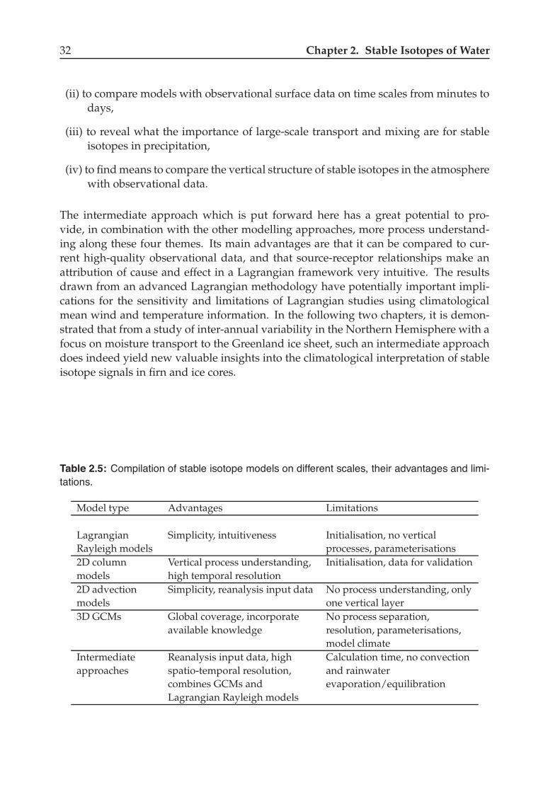
32 Chapter 2. Stable Isotopes of Water
(ii) to compare models with observational surface data on time scales from minutes todays,
(iii) to reveal what the importance of large-scale transport and mixing are for stableisotopes in precipitation,
(iv) to find means to compare the vertical structure of stable isotopes in the atmospherewith observational data.
The intermediate approach which is put forward here has a great potential to pro-vide, in combination with the other modelling approaches, more process understand-ing along these four themes. Its main advantages are that it can be compared to cur-rent high-quality observational data, and that source-receptor relationships make anattribution of cause and effect in a Lagrangian framework very intuitive. The resultsdrawn from an advanced Lagrangian methodology have potentially important impli-cations for the sensitivity and limitations of Lagrangian studies using climatologicalmean wind and temperature information. In the following two chapters, it is demon-strated that from a study of inter-annual variability in the Northern Hemisphere with afocus on moisture transport to the Greenland ice sheet, such an intermediate approachdoes indeed yield new valuable insights into the climatological interpretation of stableisotope signals in firn and ice cores.
Table 2.5: Compilation of stable isotope models on different scales, their advantages and limi-tations.
Model type Advantages Limitations
LagrangianRayleigh models
Simplicity, intuitiveness Initialisation, no verticalprocesses, parameterisations
2D columnmodels
Vertical process understanding,high temporal resolution
Initialisation, data for validation
2D advectionmodels
Simplicity, reanalysis input data No process understanding, onlyone vertical layer
3D GCMs Global coverage, incorporateavailable knowledge
No process separation,resolution, parameterisations,model climate
Intermediateapproaches
Reanalysis input data, highspatio-temporal resolution,combines GCMs andLagrangian Rayleigh models
Calculation time, no convectionand rainwaterevaporation/equilibration
Bibliography
Adams, J. W., D. Rodriguez, and R. A. Cox. 2005. The uptake of SO2 on Saharan dust: a flowtube study. Atmos. Chem. Phys. 5, 2679–2689.
Aggarwal, P. K., M. A. Dillon, and A. Tanweer. 2004. Isotope fractionation at the soil-atmosphere interface and the 18O budget of atmospheric oxygen. Geophys. Res. Lett. 31,L14202. 10.1029/2004GL019945.
Alpert, P., and E. Ganor. 1993. A jet-stream associated heavy dust storm in the western Mediter-ranean. J. Geophys. Res. 98, 7339–7349.
Andersson, E., P. Bauer, A. Beljaars, F. Chevallier, E. Holm, M. Janiskova, P. Kallberg, G. Kelly,P. Lopez, A. McNally, E. Moreau, A. J. Simmons, J.-N. Thepaut, and A. M. Tompkins. 2005.Assimilation and modeling of the atmospheric hydrological cycle in the ECMWF forecastingsystem. BAMS 82, 387–402.
Ansmann, A., J. Bosenberg, A. Chaikovsky, A. Comeron, S. Eckhardt, R. Eixmann, V. Freuden-thaler, P. Ginoux, L. Komguem, H. Linne, M. A. L. Marquez, V. Matthias, I. Mattis, V. Mitev,D. Muller, S. Music, S. Nickovic, J. Pelon, L. Sauvage, P. Sobolewsky, M. K. Srivastava,A. Stohl, O. Torres, G. Vaughan, U. Wandinger, and M. Wiegner. 2003. Long-range trans-port of Saharan dust to northern Europe: The 11–16 October 2001 outbreak observed withEARLINET. J. Geophys. Res. 108, 4783. 10.1029/2003JD003757.
Appenzeller, C., and H. C. Davies. 1992. Structure of stratospheric intrusions into the tropo-sphere. Nature 358, 570–572.
Appenzeller, C., H. C. Davies, and W. A. Norton. 1996. Fragmentation of stratospheric intru-sions. J. Geophys. Res. 101, 1435–1456.
Appenzeller, C., J. Schwander, S. Sommer, and T. Stocker. 1998a. The North Atlantic Oscillationand its imprint on precipitation and ice accumulation in Greenland. Geophys. Res. Lett. 25,1939–1942.
Appenzeller, C., T. Stocker, and M. Anklin. 1998b. North Atlantic Oscillation dynamics recordedin Greenland ice cores. Science 282, 446–449.
Araguas-Araguas, L., K. Frohlich, and K. Rozanski. 2000. Deuterium and oxygen-18 isotopecomposition of precipitation and atmospheric moisture. Hydrol. Process. 14, 1341–1355.
Avila, A., I. Queralt-Mitjans, and M. Alarcon. 1997. Mineralogical composition of African dustdelivered by red rains over northeastern Spain. J. Geophys. Res. 102, 21977–21996.
219
220 BIBLIOGRAPHY
Aymoz, G., J.-L. Jaffrezo, V. Jacob, A. Colomb, and C. George. 2004. Evolution of organic andinorganic components of aerosol during a Saharan dust episode observed in the French Alps.Atmos. Chem. Phys. 4, 2499–2512.
Barkan, J., P. Alpert, H. Kutiel, and P. Kishcha. 2005. Synoptics of dust transportation days fromAfrica toward Italy and central Europe. J. Geophys. Res. 110, D07208.
Barlow, L. K., J. C. Rogers, M. C. Serreze, and R. G. Barry. 1997. Aspects of climate variabilityin the North Atlantic sector: Discussion and relation to the Greenland Ice Sheet Project 2high-resolution isotopic signal. J. Geophys. Res. 102, 26333–26344.
Barlow, L. K., J. W. C. White, R. G. Barry, J. C. Rogers, and P. M. Grootes. 1993. The NorthAtlantic Oscillation signature in Deuterium and Deuterium excess signals in the Greenlandice sheet project 2 ice core, 1840-1970. Geophys. Res. Lett. 24, 2901–2904.
Bergametti, G., L. Gomes, C. G., P. Rognon, and M.-N. le Coustumer. 1989. African dust ob-served over Canary Islands - Source-regions identification and transport pattern for somesummer situations. J. Geophys. Res. 94, 14855–14864.
Blattmann-Singh, M. 2005. Durchfuhrung idealisierter Simulationen im regionalen KlimamodellCHRM mit einem Wasserdampftracer. B.sc. thesis. IAC, ETH Zurich.
Bleck, R., and C. Mattocks. 1984. A preliminary analysis of the role of potential vorticity inAlpine lee cyclogenesis. Contrib. Atmos. Phys. 57, 357–368.
Bonasoni, P., P. Cristofanelli, F. Calzolari, U. Bonafe, F. Evangelisti, A. Stohl, S. Zauli, R. van Din-genen, T. Colombo, and Y. Balkanski. 2004. Aerosol-ozone correlations during dust transportepisodes. Atmos. Chem. Phys. 4, 1201–1215.
Bosc, E., A. Bricaud, and D. Antoine. 2004. Seasonal and interannual variability in algal biomassand primary production in the Mediterranean Sea, as derived from 4 years of SeaWiFS obser-vations. Global Biogeochem. Cycles. 10.1029/2003GB002034.
Bosilovich, M. 2002. On the vertical distribution of local and remote sources of water for pre-cipitation. Meteorol. Atmos. Phys. 80, 31–41.
Bosilovich, M., and S. Schubert. 2002. Water vapour tracers as diagnostics of the regional hy-drologic cycle. J. Hydrometeorol. Pp. 149–165.
Bosilovich, M. G., Y. C. Sud, S. D. Schubert, and G. K. Walker. 2003. Numerical simulation ofthe large-scale North American monsoon water sources. J. Geophys. Res. 108, 8614.
Bricaud, A., E. Bosc, and D. Antoine. 2002. Algal biomass and sea surface temperature in theMediterranean Basin Intercomparison of data from various satellite sensors, and implicationsfor primary production estimates. Remote Sens. Environ. 81, 163–178.
Bromwich, D. H., Q. Chen, Y. Li, and R. I. Cullather. 1999. Precipitation over Greenland and itsrelation to the North Atlantic Oscillation. J. Geophys. Res. 104, 22103–22115.
Brown, J., and I. Simmonds. 2004. Sensitivity of the !18O-temperature relationship to the distri-bution of continents. Geophys. Res. Lett. 31, L09208.
BIBLIOGRAPHY 221
Brubaker, K. L., P. A. Dirmeyer, A. Sudradjat, B. S. Levy, and F. Bernal. 2001. A 36-yr climato-logical description of the evaporative sources of warm-season precipitation in the Mississippiriver basin. J. Hydromet. 2, 537–557.
Budyko, M. I. 1974. Climate and Life. Academic Press, San Diego.
Cappa, C. D., M. B. Hendricks, D. J. DePaolo, and R. C. Cohen. 2003. Isotopic fractionation ofwater during evaporation. J. Geophys. Res. 108, 4525.
Charles, R. D., D. Rind, J. Jouzel, R. D. Koster, and R. G. Fairbanks. 1994. Glacial-interglacialchanges in moisture sources for Greenland: Influences on the ice core record of climate. Sci-ence 263, 508–511.
Christensen, J. H., and O. B. Christensen. 2003. Severe summertime flooding in Europe. Nature421, 805–806.
Ciais, P., and J. Jouzel. 1994. Deuterium and oxygen 18 in precipitation: Isotopic model, includ-ing mixed cloud processes. J. Geophys. Res. 99, 16793–16803.
Ciais, P., J. W. C. White, J. Jouzel, and J. R. Petit. 1995. The origin of present-day Antarcticprecipitation from surface snow deuterium excess data. J. Geophys. Res. 100, 18917–18927.
Claquin, T., M. Schulz, and Y. J. Balkanski. 1999. Modeling the mineralogy of atmospheric dustsources. J. Geophys. Res. 104, 22243–22256.
Collaud Coen, M., E. Weingartner, D. Schaub, C. Hueglin, C. Corrigan, S. Henning,M. Schwikowski, and U. Baltensperger. 2004. Saharan dust events at the Jungfraujoch: detec-tion by wavelength dependence of the single scattering albedo and first climatology analysis.Atmos. Chem. Phys. 4, 2465–2480.
Craig, H., and L. I. Gordon. 1965. Deuterium and oxygen 18 variations in the ocean and themarine atmosphere. Pp. 9–130. In Stable isotopes in oceanographic studies and paleotemperatures.E. Tongiorgi (ed.). Consiglio nazionale delle ricerche, Laboratorio di geologia nucleare, Pisa.
Dahl-Jensen, D., K. Mosegaard, N. Gundestrup, G. D. Clow, S. J. Johnsen, A. Hansen, andN. Balling. 1998. Past temperatures directly from the Greenland ice sheet. Science 282, 268–271.
Dansgaard, W. 1964. Stable isotopes in precipitation. Tellus 16, 436–468.
Dansgaard, W. e. a. 1993. Evidence for past climate from a 250-kyr ice-core record. Nature 364,218–220.
Davies, H. C. 1976. A lateral boundary formulation for multi-level prediction models. Q. J. R.Mereorol. Soc. 102, 405–418.
DeFries, R. S., and J. R. G. Townshend. 1994. NDVI-derived land cover classification at globalscales. Int. J. Remote Sensing 15, 3567–3586.
Delaygue, G., V. Masson, J. Jouzel, R. D. Koster, and R. J. Healy. 2000. The origin of Antarcticprecipitation: a modelling approach. Tellus 52B, 19–36.
222 BIBLIOGRAPHY
Delmotte, M., V. Masson, J. Jouzel, and V. I. Morgan. 2000. A seasonal deuterium excess signalat Law Dome, coastal eastern Antarctica: A southern ocean signature. J. Geophys.Res. 105,7187–7197.
Dickinson, R. E. 1984. Modeling Evapotranspiration for 3-dimensional Global Climate Models. Pp. 58–72. number 29 in Geophysical Monographs. American Geophysical Union.
Dirmeyer, P. A., and K. L. Brubaker. 1999. Contrasting evaporative moisture sources during thedrought of 1988 and the flood of 1993. J. Geophys. Res. 104, 19383–19397.
Druyan, L. M., and R. D. Koster. 1989. Sources of Sahel precipitation for simulated drought andrainy seasons. J. Climate 2, 1438–1446.
Duce, R., P. S. Liss, J. T. Merrill, E. L. Atlas, P. Buatt-Menard, B. B. Hicks, J. M. Miller, J. M. Pros-pero, R. Arimoto, T. M. Church, W. Ellis, J. N. Galloway, L. Hansen, T. D. Jickells, A. H. Knap,K. H. Reinhardt, B. Schneider, A. Soudine, J. J. Tokos, S. Tsunogai, R. Wollast, and M. Zhou.1991. The atmospheric input of trace gas species to the world ocean. Global Biogeochem. Cycles5, 193–259.
DWD 1995. Dokumentation des EM/DM Systems. Deutscher Wetterdienst, Abteilung Forschung,Offenbach/Main.
Eckhardt, S., A. Stohl, H. Wernli, P. James, C. Forster, and N. Spichtinger. 2004. A 15-yearclimatology of warm conveyor belts. J. Climate 17, 218–237.
Eichler, A., M. Schwikowski, H. W. Gaggeler, V. Furrer, H.-A. Synal, J. Beer, M. Saurer, andM. Funk. 2000. Glaciochemical dating of an ice core from upper Grenzgletscher (4200 ma.s.l). J. Glaciol. 46, 507–515.
EPICA community members 2004. Eight glacial cycles from an Antarctic ice core. Nature 429,623–628.
Federer, B., B. Thalmann, and J. Jouzel. 1982a. Stable isotopes in hailstones. Part II: Embryo andhailstone growth in different storms. J. Atmos. Sci. 39, 1336–1355.
Federer, B., N. Brichet, and J. Jouzel. 1982b. Stable isotopes in hailstones. Part I: The isotopiccloud model. J. Atmos. Sci. 39, 1323–1335.
Fischer, M. J., and K. Sturm. 2006. REMOiso forcing for the iPILPS Phase 1 experiments and the.Hydrol. Process. 51, 73–89. 10.1016/j.gloplacha.2005.12.006.
Franzen, L. G., M. Hjelmroos, P. Kallberg, A. Rapp, J. O. Mattsson, and E. Brorstrom-Lunden.1995. The Saharan dust episode of south and central Europe, and northern Scandinavia,March 1991. Weather 50, 313–318.
Frei, C., J. H. Christensen, M. Deque, D. Jacob, R. G. Jones, and P. L. Vidale. 2003. Daily precipi-tation statistics in regional climate models: Evaluation and intercomparison for the EuropeanAlps. J. Geophys. Res. 108, 4124.
Fukutome, S., C. Prim, and C. Schar. 2001. The role of soil states in medium-range weatherpredictability. Nonlin. Process. Geophys. 8, 373–386.
BIBLIOGRAPHY 223
Gat, J. R. 1996. Oxygen and hydrogen isotopes in the hydrologic cycle. Annu. Rev. Earth Planet.Sci. 24, 225–262.
Gat, J. R., B. Klein, Y. Kushnir, W. Roether, H. Wernli, R. Yam, and A. Shemesh. 2003. Isotopecomposition of air moisture over the Mediterranean Sea: an index of air-sea interaction pat-tern. Tellus 55B, 953–965.
Gedzelman, S. D., and J. R. Lawrence. 1982. The isotopic composition of cyclonic precipitation.J. Appl. Meteorol. 21, 1385–1404.
Gedzelman, S. D., and J. R. Lawrence. 1990. The isotopic composition of precipitation from twoextratropical cyclones. Mon. Wea. Rev. 118, 495–509.
Gedzelman, S. D., and R. Arnold. 1994. Modeling the isotopic composition of precipitation. J.Geophys. Res. 99, 10455–10472.
Gedzelman, S. D., J. M. Rosenbaum, and J. R. Lawrence. 1989. The megalopolitan snowstormof 11-12 February 1983: Isotopic composition of the snow. J. Atmos. Sciences 46, 1637–1649.
Gedzelman, S., J. Lawrence, J. Gamache, M. Black, E. Hindman, R. Black, J. Dunion,H. Willoughby, and X. P. Zhang. 2003. Probing hurricanes with stable isotopes of rain andwater vapor. Mon. Wea. Rev. 131, 1112–1127.
Goudie, A. S., and N. J. Middleton. 2001. Saharan dust storms: nature and consequences. Earth-Sci. Rev. 56, 179–204.
Hamonou, E., P. Chazette, D. Balis, F. Dulac, X. Schneider, E. Galani, G. Ancellet, and A. Pa-payannis. 1999. Characterization of the vertical structure of Saharan dust export to theMediterranean basin. J. Geophys. Res. 104, 22257–22270.
Hanna, E., P. Valdes, and J. McConnell. 2001. Patterns and variations of snow accumulation overGreenland, 1979-98, from ECMWF analyses, and their verification. J. Climate 14, 3521–3535.
Hecht, M. W., W. R. Holland, and P. J. Rasch. 1995. Upwind-weighted advection schemes forocean tracer transport: An evaluation in a passive tracer context. J. Geophys. Res. 100, 20763–20778.
Heck, P., D. Luethi, H. Wernli, and C. Schaer. 2001. Climate impacts of European-scale anthro-pogenic vegetation changes: A sensitivity study using a regional climate model. J. Geophys.Res. 106, 7817–7835.
Helsen, M. M. 2005. On the interpretation of stable isotopes in Antarctic precipitation. PhD Thesis,Utrecht University.
Helsen, M. M., R. S. W. van de Wal, M. R. van den Broeke, E. R. T. Kerstel, V. Masson-Delmotte,H. A. J. Meijer, C. H. Reijmer, and M. P. Scheele. 2004. Modelling the isotopic composition ofsnow using backward trajectories: a particular precipitation event in Dronning Maud Land,Antarctica. Ann. Glaciol. 39, 293–299.
224 BIBLIOGRAPHY
Helsen, M. M., R. S. W. van de Wal, M. R. van den Broeke, V. Masson-Delmotte, H. A. J. Meijer,M. P. Scheele, and M. Werner. 2005a. Modelling the isotopic composition of Antarctic snowusing backward trajectories: Simulation of snow pit records. J. Geophys. Res. Pp. submitted.
Helsen, M. M., R. W. van de Wal, M. van den Broeke, D. van As, H. Meijer, and C. Reijmer.2005b. Oxygen isotope variability in snow from western Dronning Maud Land, Antarcticaand its relation to temperature. Tellus 57B, 423–435.
Henning, S., E. Weingartner, M. Schwikowski, H. W. Gaeggeler, R. Gehrig, K.-P. Hinz, A. Trim-born, B. Spengler, and U. Baltensperger. 2003. Seasonal variation of water-soluble ionsof the aerosol at the high-alpine site Jungfraujoch (3580 m asl). J. Geophys. Res. 108, 4030.10.1029/2002JD002439.
Hinz, K.-P., A. Trimborn, E. Weingartner, S. Henning, U. Baltensperger, and B. Spengler. 2005.Aerosol single particle composition at the Jungfraujoch. J. Aerosol Sci. 36, 123–145.
Hoerling, M., and A. Kumar. 2003. The perfect ocean for drought. Science 299, 691–694.
Hoffmann, G., J. Jouzel, and V. Masson. 2000. Stable water isotopes in atmospheric generalcirculation models. Hydrol. Process. 14, 1385–1406.
Hoffmann, G., M. Werner, and M. Heimann. 1998. Water isotope module of the ECHAM at-mospheric general circulation model: A study on timescales from days to several years. J.Geophys. Res. 103, 16871–16896.
Holzer, M., T. M. Hall, and R. B. Stull. 2005. Seasonality and weather-driven variability oftranspacific transport. J. Geophys. Res. 110, D23103.
Houghton, J. T., Y. Ding, D. J. Griggs, M. Noguer, P. J. van der Linden, and D. Xiaosu. (Eds.) 2001.Climate Change 2001: The Scientific Basis. Contribution of Working Group I to the Third AssessmentReport of the Intergovernmental Panel on Climate Change (IPCC). Cambridge University Press,UK.
Houze Jr., R. A. 1993. Cloud Dynamics. Academic Press, San Diego.
Huebert, B. J., B. W. Blomquist, J. E. Hare, C. W. Fairall, J. E. Johnson, and T. S. Bates. 2004.Measurement of the air-sea DMS flux and transfer velocity using eddy correlation. Geophys.Res. Lett. 31, L23113. 10.1029/2004GL021567.
Hurrell, J. W. 1995. Decadal trends in the North Atlantic oscillation: Regional temperatures andprecipitation. Science 269, 676–679.
Hurrell, J. W., Y. Kushir, G. Ottersen, and M. Visbeck. 2003. The North Atlantic Oscillation. number134 in Geophysical Monographs. American Geophysical Union, Washington, USA.
Jacobsen, I., and E. Heise. 1982. A new economic method for the computation of the surfacetemperature in numerical models. Beitr. Phys. Atmos. 55, 128–141.
James, P., A. Stohl, N. Spichtinger, S. Eckhardt, and C. Forster. 2004. Climatological aspectsof the extreme European rainfall of August 2002 and a trajectory method for estimating theassociated evaporative source regions. NHESS 4, 733–746.
BIBLIOGRAPHY 225
Johnsen, S. J., W. Dansgaard, and J. W. C. White. 1989. The origin of Arctic precipitation underpresent and glacial conditions. Tellus 41B, 452–468.
Jones, C., N. Mahowald, and C. Luo. 2003. The role of easterly waves on African desert dusttransport. J. Climate 16, 3617–3628.
Jordan, C. E., J. E. Dibb, B. E. Anderson, and H. E. Fuelberg. 2003. Uptake of nitrate and sulfateon dust aerosols during TRACE-P. J. Geophys. Res. 108, 8817. 10.1029/2002JD003101.
Joussaume, J., R. Sadourny, and J. Jouzel. 1984. A general circulation model of water isotopecycles in the atmosphere. Nature 311, 24–29.
Joussaume, S., R. Sadourny, and C. Vignal. 1986. Origin of precipitating water in a numericalsimulation of July climate. Ocean-Air Interact. 1, 43–56.
Jouzel, J., and L. Merlivat. 1984. Deuterium and oxygen 18 in precipitation, modelling of theisotopic effects during snow formation. J. Geophys. Res. 89, 11749–11757.
Jouzel, J., and R. D. Koster. 1996. A reconsideration of the inital conditions used for stable waterisotope models. J. Geophys. Res. 101, 22933–22938.
Jouzel, J., L. Merlivat, and E. Roth. 1975. Isotopic study of hail. J. Geophys. Res. 80, 5015–5030.
Jouzel, J., R. B. Alley, K. M. Cuffey, W. Dansgaard, P. Grootes, G. Hoffmann, S. J. Johnsen, R. D.Koster, D. Peel, C. A. Shuman, M. Stievenard, M. Stuiver, and J. White. 1997. Validity of thetemperature reconstruction from water isotopes in ice cores. J. Geophys. Res. 102, 26471–26487.
Kavanaugh, J. L., and K. M. Cuffey. 2003. Space and time variation of d18O and dD in Antarcticprecipitation revisited. Global Biogeochem. Cycles 17, 1017. 10.1029/2002GB001910.
Keil, C., H. Volkert, and D. Majewski. 1999. The Oder flood in July 1997: Transport routes ofprecipitable water diagnosed with an operational forecast model. Geophys. Res. Lett. 26, 235–238.
Kessler, E. 1969. On the distribution and continuity of water substance in atmospheric circulations.number 10 in Meteorological Monographs. American Geophysical Union.
Knippertz, P., A. H. Fink, A. Reiner, and P. Speth. 2003. Three late summer/early autumn casesof tropical-extratropical interactions causing precipitation in northwest Africa. Mon. Wea. Rev.131, 116–135.
Koren, I., and Y. J. Kaufman. 2004. Direct wind measurements of Saharan dust events from Terraand Aqua satellites. Geophys. Res. Lett. 31, L06122. 10.1029/2003GL019338.
Koster, R. D., J. Jouzel, R. J. Suozzo, and G. L. Russell. 1992. Origin of July Antarctic precipitationand its influence on deuterium content: a GCM analysis. Climate Dynamics 7, 195–203.
Koster, R., J. Jouzel, R. Souzzo, G. Russell, W. Broecker, D. Rind, and P. Eagleson. 1986. Globalsources of local precipitation as determined by the NASA/GISS GCM. Geophys. Res. Lett. 13,121–124.
226 BIBLIOGRAPHY
Krinner, G., and M. Werner. 2003. Impact of precipitation seasonality changes on isotopic signalsin polar ice cores: a multi-model analysis. Earth Plan. Sci. Lett. 216, 525–538.
Krinner, G., C. Genthon, and J. Jouzel. 1997. GCM analysis of local influences on ice core dsignals. Geophys. Res. Lett. 24, 2825–2828.
Lawrence, J. R., and S. D. Gedzelman. 1996. Low stable isotope ratios of tropical cyclone rains.Geophys. Res. Lett. 23, 527–530.
Lawrence, J. R., S. D. Gedzelman, X. Zhang, and R. Arnold. 1998. Stable isotope ratios of rainand vapor in 1995 hurricanes. J. Geophys. Res. 103, 11381–11400.
Leon, J.-F., D. Tanre, J. Pelon, Y. J. Kaufman, J. M. Haywood, and B. Chatenet. 2003. Profilingof a Saharan dust outbreak based on a synergy between active and passive remote sensing. J.Geophys. Res. 108, 8575. 10.1029/2002JD002774.
Lin, S.-J., and R. B. Rood. 1996. Multidimensional flux form semi-Lagrangian transport schemes.Mon. Wea. Rev. 124, 2046–2070.
Lin, Y.-L., R. D. Farley, and H. D. Orville. 1983. Bulk parameterization of the snow field in acloud model. J. Climate Appl. Meteor. 22, 1065–1092.
Loewe, E. 1936. The Greenland ice cap as seen by a meteorologist. Quart. J. Roy. Meteorol. Soc.62, 359–377.
Louis, J.-F. 1979. A parametric model of vertical eddy fluxes in the atmosphere. Bound.-LayerMeteorol. 17, 187–202.
Louis, J.-F., M. Tiedtke, and J. F. Geleyn. 1982. A short history of the operational PBL parameter-ization at ECMWF. Proceedings of the ECMWF Workshop on Boundary Layer Parameterizations.ECMWF. Reading, UK. Pp. 59–79.
Luthi, D., A. Cress, H. C. Davies, C. Frei, and C. Schar. 1996. Interannual variability and regionalclimate simulations. Theor. Appl. Climatol. 53, 185–209.
Mahowald, N. M., and J.-L. Dufresne. 2004. Sensitivity of TOMS aerosol index to boundary layerheight: Implications for detection of mineral aerosol sources. Geophys. Res. Lett. 31, L03103.10.1029/2003GL018865.
Majewski, D. 1991. The Europa-Model of the Deutscher Wetterdienst. Proceedings of the ECMWFWorkshop on Boundary Layer Parameterizations. Vol. 2 of ECMWF Proceedings of numerical meth-ods in atmospheric models. ECMWF. Reading, UK. Pp. 147–191.
Majoube, M. 1971. Fractionnement en oxygene 18 et en deuterium entre l’eau et sa vapeur. J.Chem. Phys. 10, 1423–1436.
Marsh, T. J., and R. B. Bradford. 2003. The floods of August 2002 in central Europe. Weather 58,168.
BIBLIOGRAPHY 227
Martius, O., E. Zenklusen, C. Schwierz, , and H. C. Davies. 2006. Episodes of Alpine heavy pre-cipitation with an overlying elongated stratospheric intrusion: A Climatology. Int. J. Climatol.26, 1149–1164. 10.1002/joc.1295.
Massacand, A. C., H. Wernli, and H. C. Davies. 1998. Heavy precipitation on the Alpine south-side: An upper-level precursor. Geophys. Res. Lett. 25, 1435–1438.
Masson-Delmotte, V., A. Landais, M. Stievenard, O. Cattani, S. Falourd, J. Jouzel, S. J. Johnsen,D. Dahl-Jensen, A. Sveinsbjornsdottir, J. W. C. White, T. Popp, and H. Fischer. 2005a.Holocene climatic changes in Greenland: Different deuterium excess signals at GreenlandIce Core Project (GRIP) and NorthGRIP. J. Geophys. Res. 110, D14102.
Masson-Delmotte, V., J. Jouzel, A. Landais, M. Stievenard, S. J. Johnsen, J. W. C. White,M. Werner, A. Sveinbjornsdottir, and K. Fuhrer. 2005b. GRIP deuterium excess reveals rapidand orbital-scale changes in Greenland moisture origin. Science 309, 118–121.
Mattis, I., A. Ansmann, D. Mueller, U. Wandinger, and D. Althausen. 2002. Dual-wavelengthRaman lidar observations of the extinction-to-backscatter ratio of Saharan dust. Geophys. Res.Lett. 20, 20. 10.1029/2002GL014721.
Mellor, G. L., and T. Yamada. 1974. A hierarchy of turbulent closure models for planetaryboundary layers. J. Atmos. Sci. 31, 1791–1806.
Merlivat, L., and J. Jouzel. 1979. Global climatic interpretation of the Deuterium-Oxygen 18relationship for precipitation. J. Geophys. Res. 84, 5029–5033.
Mladek, R., J. Barckicke, P. Binder, P. Bougeault, N. Brzovic, C. Frei, J. F. Geleyn, J. Hoffman,W. Ott, T. Paccagnella, P. Patruno, P. Pottier, and A. Rossa. 2000. Intercomparison and eval-uation of precipitation forecasts for MAP seasons 1995 and 1996. Meteorol. Atmos. Phys. 72,111–129.
Mook, W. M. E. 2001. Environmental Isotopes in he Hydrological Cycle. Principles and Applications.UNESCO/IAEA Series, http://www.-naweb.iaea.org/napc/ih/volumes.asp.
Morgenstern, O., and H. C. Davies. 1999. Disruption of an upper-level PV-streamer by oro-graphic and cloud-diabatic effects. Contr. Atmos. Phys. 72, 173–186.
Mosley-Thompson, E., C. R. Readinger, P. Craigmil, L. G. Thompson, and C. A. Calder. 2005. Re-gional sensitivity of Greenland precipitation to NAO variability. Geophys. Res. Lett. 32, L24707.
Moulin, C., C. E. Lambert, U. Dayan, V. Masson, M. Ramonet, P. Bousquet, M. Lagrand, Y. J.Balkanski, W. Guelle, B. Marticorean, G. Bergametti, and F. Dulac. 1998. Satellite climatologyof African dust transport in the Mediterranean atmosphere. J. Geophys. Res. 103, 13137–13144.
Newell, R. E., N. E. Newell, Y. Zhu, and C. Scott. 1992. Tropospheric rivers? - A pilot study.Geophys. Res. Lett. 12, 2401–2404.
Noone, D., and I. Simmonds. 2002. Annular variations in moisture transport mechanisms andthe abundance of d18O in Antarctic snow. J. Geophys. Res. 107, 4742.
228 BIBLIOGRAPHY
Numaguti, A. 1999. Origin and recycling processes of precipitating water over the Eurasiancontinent: Experiments using an atmospheric general circulation model. J. Geophys.Res. 104,1957–1972.
O’Dowd, C. D., M. C. Facchini, F. Cavalli, D. Ceburnis, M. Mircea, S. Decesari, S. Fuzzi, Y. J.Yoon, and J.-P. Putaud. 2004. Biogenically driven organic contribution to marine aerosol.Nature 431, 676–680.
O’Reilly, J. E., S. Maritorena, B. G. Mitchell, D. A. Siegel, K. L. Carder, S. A. Garver, M. Kahru,and C. McClain. 1998. Ocean color chlorophyll algorithms for SeaWiFS. J. Geophys. Res. 103,24937–24953.
ornexl, B. E., M. Gehre, R. Hofling, and R. A. Werner. 1999. On-line delta O-18 measurement oforganic and inorganic substances. Rapid Comm. Mass Spectr. 13, 1685–1693.
Osada, K., H. Iida, M. Kido, K. Matsunaga, and Y. Iwasaka. 2004. Mineral dust layers in snow atMount Tateyama, Central Japan: formation processes and characteristics. Tellus 56B, 382–392.
Papayannis, A., D. Balis, V. Amiridis, G. Chourdakis, G. Tsaknakis, C. Zerefos, A. D. A. Cas-tanho, S. Nickovic, S. Kazadzis, and J. Grabowski. 2005. Measurements of Saharan dustaerosols over the Eastern Mediterranean using elastic backscatter-Raman lidar, spectropho-tometric and satellite observations in the frame of the EARLINET project. Atmos. Chem. Phys.5, 2065–2079.
Petit, J. R., J. W. C. White, N. W. Young, J. Jouzel, and Y. S. Korotkevich. 1991. Deuterium excessin recent Antarctic snow. J. Geophys. Res. 96, 5113–5122.
Preunkert, S., D. Wagenbach, M. Legrand, , and C. Vincent. 2000. Col du Dome (Mt Blanc Massif,French Alps) suitability for ice-core studies in relation with past atmospheric chemistry overEurope. Tellus 52B, 993–1012.
Prodi, F., and G. Fea. 1978. Transport and deposition of Saharan dust over Alps. Proceedings der15. Internationalen Tagung fur Alpine Meteorologie. Vol. 40. Grindelwald. Pp. 179–182.
Prodi, F., and G. Fea. 1979. A case of transport and deposition of Saharan dust over the Italianpeninsula and southern Europe. J. Geophys. Res. 84, 6951–6960.
Prospero, J. M., and P. J. Lamb. 2003. African droughts and dust transport to the Caribbean:Climate change implications. Science 302, 1024–1027.
Ravi, S., P. D’Odrioco, T. M. Over, and T. M. Zobeck. 2004. On the effect of air humidity onsoil susceptibility to wind erosion: The case of air-dry soils. Geophys. Res. Lett. 31, L09501.10.1029/2004GL019485.
Reale, O., L. Feudale, and B. Turato. 2001. Evaporative moisture sources during a sequence offloods in the Mediterranean region. Geophys. Res. Lett. 28, 2085–2088.
Robasky, F. M., and D. H. Bromwich. 1994. Greenland precipitation estimates from the atmo-spheric moisture budget. Geophys. Res. Lett. 21, 2495–2498.
BIBLIOGRAPHY 229
Rogers, J. C., J. F. Bolzan, and V. A. Pohjola. 1998. Atmospheric circulation variability associatedwith shallow-core seasonal isotopic extremes near Summit, Greenland. J. Geophys. Res. 103,11205–11219.
Rouault, M., P. Florenchie, N. Fauchereau, and C. J. C. Reason. 2003. South East tropical Atlanticwarm events and southern African rainfall. Geophys. Res. Lett. 30, 8009.
Rozanski, K., and C. Sonntag. 1982. Vertical distribution of deuterium in atmospheric watervapour. Tellus 34, 135–141.
Rozanski, K., C. Sonntag, and K. O. Munnich. 1982. Factors controlling stable isotope composi-tion of European precipitation. Tellus 34, 142–150.
Rozanski, K., L. Araguas-Araguas, and R. Gonfiantini. 1993. Isotopic patterns in modern globalprecipitation. Pp. 1–37. In Climate Change in Continental Isotopic Records. S. et al. (ed.). Geo-physical Monographs. American Geophysical Union.
Russell, G. L., and J. A. Lerner. 1981. A new finite-differencing scheme for the tracer transportequation. J. App. Met. 20, 1483–1498.
Ryall, D. B., R. G. Derwent, A. J. Manning, A. L. Redington, J. Corden, W. Millington, P. G.Simmonds, S. O’Dotherty, N. Carslaw, and G. W. Fuller. 2002. The origin of high particulateconcentrations over the United Kingdom, March 2000. Atmos. Env. 36, 1363–1378.
Saurer, M., I. Robertson, R. Siegwolf, and M. Leuenberger. 1998. Oxygen isotope analysis ofcellulose: An interlaboratory comparison. Analyt. Chem. 70, 2074–2080.
Schar, C. 2002. Numerische Methoden in der Umweltphysik. IACETH, ETH Zurich.
Schar, C., D. Luthi, U. Beyerle, and E. Heise. 1999. The soil precipitation feedback: A processstudy with a regional climate model. J. Climate 12, 722–741.
Schar, C., P. L. Vidale, D. Luthi, C. Frei, C. Haberli, M. A. Liniger, and C. Appenzeller. 2004.The role of increasing temperature variablility in European summer heatwaves. Nature 427,332–336.
Scherrer, S. C., M. Croci-Maspoli, C. Schwierz, and C. Appenzeller. 2006. Two-dimensionalindices of atmospheric blocking and their statistical relationship with winter climate patternsin the Euro-Atlantic region. Int. J. Climatol. 26, 233–249.
Schmidli, J., C. Schmutz, C. Frei, H. Wanner, and C. Schaer. 2002. Mesoscale precipitation vari-ability in the region of the European Alps during the 20th century. Int. J. Climatol. 22, 1049–1074.
Schmidt, G. A. 1999. Forward modeling of carbonate proxy data from planktonic foraminiferausing oxygen isotope tracers in a global ocean model. Palaeooceanography 14, 482–497.
Schoenfeldt, H.-J., and S. von Loewis. 2003. Turbulence-driven saltation in the atmosphericsurface layer. Meteorol. Z. 12, 257–268.
230 BIBLIOGRAPHY
Schutz, L., and M. Sebert. 1987. Mineral aerosols and source identification. J. Aerosol Sci. 18,1–10.
Schwierz, C. 2001. Interactions of Greenland-scale orography and extra-tropical synoptic-scale flow.Diss. eth no. 14356. IACETH, ETH Zurich.
Schwikowski, M., P. Seibert, U. Baltensperger, and H. W. Gaggeler. 1995. A study of an out-standing Saharan dust event at the high-alpine site Jungfraujoch, Switzerland. Atmos. Env.15, 1829–1842.
Seimon, A. 2003. Improving climatic signal representation in tropical ice cores: A case studyfrom the Quelccaya Ice Cap, Peru. Geophys. Res. Lett. 30, 1772.
Seneviratne, S. I., J. S. Pal, E. A. B. Eltahir, and C. Schaer. 2002. Summer dryness in a warmerclimate: a process study with a regional climate model. Climate Dynamics 20, 69–85.
Shao, Y., and L. M. Leslie. 1997. Wind erosion prediction over the Australian continent. J. Geo-phys. Res. 102, 30091–30105.
Simmonds, A. J., and J. K. Gibson. 2000. The ERA-40 Project Plan. ECMWF. Shinfield Park,Reading, UK.
Simmons, A. J., and D. M. Burridge. 1981. An energy and angular-momentum conserving ver-tical finite-difference scheme and hybrid vertical coordinates. Mon. Wea. Rev. 109, 758–766.
Smolarkiewicz, P. K. 2005. Multidimensional positive defnite advection transport algorithm:An overview. Int. J. Numer. Meth. Fluids Pp. 1–22.
Smolarkiewicz, P. K., and L. G. Margolin. 1998. MPDATA: A finite-difference solver for geo-physical flows. J. Comput. Phys. 140, 459–480.
Smolarkiewicz, P. K., and W. W. Grabowski. 1990. The multidimensional positive definite ad-vection transport algorithm - nonoscillatory option. J. Comput. Phys. 86, 355–375.
Sodemann, H. 2000. Relationships between the Origin of Air Masses and Carbon Monoxide Measure-ments at the Cape Point Trace Gas Monitoring Station. B.sc. (hons) thesis. University of CapeTown, SA. Department of Environmental and Geographical Science.
Sodemann, H., A. Palmer, C. Schwierz, M. Schwikowski, and H. Wernli. 2006. The transporthistory of two Saharan dust events archived in an Alpine ice core. Atmos. Chem. Phys. 6, 667–688.
Sodemann, H., and T. Foken. 2005. Special characteristics of the temperature structure near thesurface. Theor. Appl. Climatol. 80, 81–89.
Steig, E. J., P. M. Grootes, and M. Stuiver. 1994. Seasonal precipitation timing and ice corerecords. Science 266, 1885–1886.
Steinacker, R. 1984. The isentropic vorticity and the flow oer and around the Alps. Riv. Met. Aer.43, 79–83.
BIBLIOGRAPHY 231
Stohl, A. 1998. Computation, accuracy, and applications of trajectories - a review and bibliogra-phy. Atmos. Env. 32, 947–966.
Stohl, A., and P. James. 2004. A Lagrangian analysis of the atmospheric branch of the globalwater cycle. Part I: Method description, validation, and demonstration for the August 2002flooding in Central Europe. J. Hydrometeorol. 5, 656– 678.
Stohl, A., and P. James. 2005. A Lagrangian analysis of the atmospheric branch of the globalwater cycle. Part II: Moisture transports between Earth’s ocean basins and river catchments.J. Hydrometeorol. 6, 961–984.
Stuiver, M., and M. Grootes. 2000. GISP-2 oxygen-isotope ratios.. Quatern. Res. 53, 277–284.
Sturm, K., G. Hoffmann, B. Langmann, and W. Stichler. 2005. Simulation of d18O in precipita-tion by the regional. Glob. Planet. Change 19, 3425–3444.
Tafferner, A. 1990. Lee cyclogenesis resulting from the combined outbreak of cold air and po-tential vorticity against the Alps. Meteorol. Atmos. Phys. 43, 31–47.
Takacs, L. L. 1985. A two-step scheme for the advection equation with minimized dissipationand dispersion errors. Mon. Wea. Rev. 113, 1050–1065.
Tegen, I., and I. Fung. 1994. Modeling of mineral dust in the atmosphere: Sources, transport,and optical thickness. J. Geophys. Res. 99, 22897–22914.
Temperton, C. 1988. Implicit normal mode initialization. Mon. Wea. Rev. 116, 1013–1033.
Tiedtke, M. 1989. A comprehensive mass flux scheme for cumulus parameterization in large-scale models. Mon. Wea. Rev. 117, 1779–1800.
Trenberth, K. E. 1997. Using atmospheric budgets as a constraint on surface fluxes. J. Climate 10,2796–2809.
Troen, I., and L. Mahrt. 1986. A simple model of the atmospheric boundary-layer - Sensitivityto surface evaporation. Bound.-Layer Meteorol. 37, 129–148.
Ulbrich, U., T. Bruecher, A. H. Fink, G. C. Leckebusch, A. Krueger, and J. G. Pinto. 2003a. Thecentral European floods of August 2002: Part 1 - Rainfall periods and flood development.Weather 58, 371–377.
Ulbrich, U., T. Bruecher, A. H. Fink, G. C. Leckebusch, A. Krueger, and J. G. Pinto. 2003b. Thecentral European floods of August 2002: Part 2 - Synoptic causes and considerations withrespect to climatic change. Weather 58, 434–442.
van Bebber, W. J. 1891. Die Zugstrassen der barometrischen Minima nach den Bahnenkartender Deutschen Seewarte von 1987–1890. Meteorol. Z. 8, 361–366.
van Loon, H., and J. C. Rogers. 1978. Seesaw in winter temperatures between Greenland andNorthern Europe. 1. General description. Mon. Wea. Rev. 106, 296–310.
Vidale, P. L., D. Luethi, C. Frei, S. I. Seneviratne, and C. Schar. 2003. Predictability and uncer-tainty in a regional climate model. J. Geophys. Res. 108, 4586.
232 BIBLIOGRAPHY
Vidale, P. L., D. Luthi, P. Heck, C. Schar, and C. Frei. 2002. The Development of Climate HRM(ex-DWD EM). IACETH, ETH Zurich.
Vinther, B. M., S. J. Johnsen, K. K. Andersen, H. B. Clausen, and A. W. Hansen. 2003. NAOsignal recorded in the stable isotopes of Greenland ice cores. Geophys. Res. Lett. 30, 1387.10.1029/2002GL016193.
Wagenbach, D., and K. Geis. 1989. The mineral dust record in a high altitude Alpine glacier(Colle Gnifetti, Swiss Alps). Pp. 543–564. In Paleoclimatology and Paleometeorology: Modern andPast Patterns of Global Atmospheric Transport. M. Leinen, and R. Sarnthein. (Eds.). Kluwer Aca-demic Publishers.
Walker, G. T., and E. W. Bliss. 1928. World weather IV: Some applications to seasonal foreshad-owing. Mem. Roy. Meteorol. Soc. 3, 81–95.
Werner, M., M. Heimann, and G. Hoffman. 2001. Isotopic composition and origin of polarprecipitation in present and glacial climate simulations. Tellus 53B, 53–71.
Wernli, H. 1995. Lagrangian perspectives of extratropical cyclogenesis. Diss. eth no. 11016. IACETH,ETH Zurich.
Wernli, H. 1997. A Lagrangian-based analysis of extratropical cyclones. II: A detailed case-study. Q. J. R. Meteorol. Soc. 123, 1677–1706.
Wernli, H., and H. C. Davies. 1997. A Lagrangian-based analysis of extratropical cyclones. I:The method and some applications. Q. J. R. Meteorol. Soc. 123, 467–489.
Wernli, H., S. Dirren, M. Liniger, and M. Zillig. 2002. Dynamical aspects of the life cycle of thewinter storm ’Lothar’. Q. J. R. Meteorol. Soc. 128, 405–429.
White, J. W. C., L. K. Barlow, D. Fisher, P. Grootes, J. Jouzel, S. J. Johnsen, M. Stuiver, andH. Clausen. 1997. The climate signal in the stable isotopes of snow from Summit, Greenland:Results of comparisons with modern climate observations. J. Geophys. Res. 102, 26425–26439.
Yoshimura, K., T. Oki, and K. Ichiyanagi. 2004. Evaluation of two-dimensional atmosphericwater circulation fields in reanalyses by using precipitation isotopes databases. J. Geophys.Res. 109, D20109.
Yoshimura, K., T. Oki, N. Ohte, and S. Kanae. 2003. A quantitative analysis of short-term 18Ovariability with a Rayleigh-type isotope circulation model. J. Geophys. Res. 108, 4647.
Zangl, G. 2004. Numerical simulations of the 12-13 August 2002 flooding event in eastern Ger-many. Q. J. R. Meteorol. Soc. 130, 1921 – 1940.