standard for ground vehicle mobility - dtic

M

US Army Corpsof Engineers ®Engineer Research andDevelopment Center

Standard for Ground Vehicle MobilityE. Alex Baylot, Jr., Burhman Q. Gates, John G. Green, February 2005Paul W. Richmond, Niki C. Goerger, George L. Mason,Chris L. Cummins, and Laura S. Bunch

0 f

Apoefopu birees;dsrbtoisulme.

ERDC/GSL TR-05-6February 2005

Standard for Ground Vehicle MobilityE. Alex Baylot, Jr., Burhman Q. Gates, John G. Green,Paul W. Richmond, Niki C. Goerger, George L. Mason,and Chris L. Cummins

Geotechnical and Structures LaboratoryU.S. Army Engineer Research and Development Center3909 Halls Ferry RoadVicksburg, MS 39180-6199

Laura S. Bunch

North Wind, Inc.3046 Indiana Ave.Suite R, PMB 172Vicksburg, MS 39180-5252

Final report

Approved for public release; distribution is unlimited

20050421 058Prepared for Office of Assistant Secretary of the Army for Acquisition,

Logistics, and TechnologyWashington, DC 20310

ABSTRACT: Mobility implementation in military models and simulations (M&S) currently is tailored primar-ily for specific models, leading to inconsistency between models. To assist decision-makers in analysis, acquisition,and training activities, it is necessary to provide and promote consistency among the models.

The NATO Reference Mobility Model (NRMM), Version II, is the Army Battle Command, Simulation and Ex-perimentation Directorate, standard for single vehicle ground movement representation. This report describes thedevelopment of an NRMM-based Standard Mobility (STNDMob) Application Programming Interface (API) as ameans of readily achieving higher fidelity movement representation by incorporating terrain-limited speeds intoM&S.

As described in the report, the STNDMob API, Version 3, includes descriptions of two derivative models: thelow-resolution (Level 1) and the medium-resolution (Level 2) capabilities of STNDMob within the tactical/entityfidelity. Each level of resolution has two degrees of fidelity. These levels of resolution are an implementation of thephysical models for steady-state speed conditions. As a whole, STNDMob can be classified as a service module thatprovides vehicle speeds to a vehicle routing service/planner.

Included in the report are descriptions of the input/output data, algorithm process and supporting equations, andexample data. Appendixes provide supporting data descriptions, software documentation, and a comparison ofSTNDMob to NRMM.

DISCLAIMER: The contents of this report are not to be used for advertising, publication, or promotional purposes.Citation of trade names does not constitute an official endorsement or approval of the use of such commercial products.All product names and trademarks cited are the property of their respective owners. The findings of this report are notto be construed as an official Department of the Army position unless so designated by other authorized documents.

DESTROY THIS REPORT WHEN IT IS NO LONGER NEEDED. DO NOT RETURN TO THE ORIGINATOR.

Contents

Conversion Factors, Non-SI to SI Units of Measurement ............................... vi

Preface ................................................................................................................. vii

1- Introduction ...................................................................................................... 1

Overview ............................................................................................................ 1Scope ........................................................................................................ 3

2- Low -Resolution M obility M odeling (Level 1) .......................................... 4

Overview ...................................................................................................... .4Input Data ..................................................................................................... 5

Terrain ....................................................................................................... 5Vehicle ..................................................................................................... 6

Process ...................................................................................................... 7Representative vehicles and preset terrain (Fidelity Degree 1) ................. 7Specific vehicles and preset terrain (Fidelity Degree 2) ................................. 8

Output .......................................................................................................... 11Data tables .............................................................................................. 11Vehicle data ............................................................................................ 12

Exam ple Output .......................................................................................... 13Representative vehicles and preset terrain (Level 1, Fidelity 1) ............. 13Specific vehicles and preset terrain (Fidelity 2) ..................................... 13

3- Medium-Resolution Mobility Modeling (Level 2) ................................... 14

Input Data ................................................................................................... 14Terrain ..................................................................................................... 14Vehicle ..................................................................................................... 15

Process .......................................................................................................... 17Description .............................................................................................. 17Physical m odel ....................................................................................... 17

Behavioral M odel ....................................................................................... 35Exam ple Output .......................................................................................... 36

Representative vehicles and variable terrain (Level 2, Fidelity 3) ....... 36Specific vehicles and variable terrain (Level 2, Fidelity 4) ..................... 37

4- Sum m ary ................................................................................................... 38

iii

R eferences ............................................................................................................ 40

Appendix A: Generation of Mobility Speed Predictions ................................ Al

Appendix B: WARSIM Terrain Common Data Model (TCDM) STGJto M LU M appings ..................................................................... B I

Appendix C: Vehicle Data, Fidelity 3 and 4 ................................................... CI

Appendix D: Comparison of NRMM and STNDMob .................................... DI

SF 298

List of Figures

Figure I. I. The suite of STNDMob APIs will span the hierarchy withexpanded degrees of fidelity in the tactical/entity hierarchylevel based on terrain and vehicle data ...................................... 2

Figure 1.2. Structure of model hierarchy ..................................................... 3

Figure 3. 1. Comparison of tractive force required and tractive forceavailab le ..................................................................................... 18

Figure 3.2. Traction-required relationships under slippery conditionsfor the given soil group for a vehicle as a function of soilstrength and vehicle speed ......................................................... 20

Figure 3.3. Friction circle, with forces in coefficient form .......................... 26

Figure 3.4. Free-body diagram ..................................................................... 30

Figure 3.5. Plot of maximum vehicle speeds for the AASHOalgorithm in N RM M .................................................................. 31

Figure 3.6. Comparison of the "bicycle" model with the NRMMA SHAT02 algorithm ................................................................ 34

List of Tables

Table 2. 1. Vehicle Bins and Representative Vehicles with Mappings ....... 6

Table 2.2. File Inform ation ......................................................................... I I

Table 2.3. Definition of Index Values ........................................................ 12

Table 2.4. V ehicle Inform ation ................................................................... 12

iv

Table 2.5. Predictions for High-Mobility Tracked Vehicle ....................... 13

Table 2.6. Predictions for a T-80 Tank ...................................................... 13

Table 3.1. Coefficient of Rolling Resistance ............................................. 21

Table 3.2. Description of Effects to Be Modeled During a TurningM aneuver ................................................................................. 25

Table 3.3. On-Road Friction Coefficients Available for Use inN R M M ..................................................................................... 26

Table 3.4. AASHO Maximum Speeds Used in NRMM ............................ 31

Table 3.5. Example of High-Mobility Tracked Vehicle ............................ 37

Table 3.6. Example of T-72 Tank ............................................................. 37

Conversion Factors, Non-SIto SI Units of Measurement

Non-SI units of measurement used in this report can be converted to SI unitsas follows:

Multiply By To Obtainfeet 0.3048 metershorsepower (550 foot-pounds 745.6999 watts(force) per second)inches 25.4 millimetersmiles (U.S. statute) 1.609347 kilometerspounds (mass) 0.4535924 kilogramstons (2,000 pounds, mass) 907.1847 kilograms

vi

Preface

The research reported herein was conducted under the sponsorship of theOffice of the Assistant Secretary of the Army for Acquisition, Logistics, andTechnology under the 62784/T40/154 project element from fiscal years 2000to 2003. The project was executed in partnership with the U.S. Army Trainingand Doctrine Command Analysis Center (TRAC) COMBATxx' simulation teamunder the guidance of the Army Battle Command, Simulation, andExperimentation Directorate (BCSED). The authors would like to acknowledgethe contributions of the COMBATxx' team, particularly Mr. Dave Durda andMAJ Simon R. Goerger, regarding design and implementation for theCOMBATxxl simulation model.

This research was conducted by personnel of the U.S. Army EngineerResearch and Development Center's (ERDC) Geotechnical and StructuresLaboratory (GSL) and North Wind, Inc. Work was conducted under the generalsupervision of Dr. David W. Pittman, Director, GSL; Dr. Albert J. Bush III,Chief, GSL Engineering Systems and Materials Division; and Dr. William E.Willoughby, Acting Chief, GSL Mobility Systems Branch (MSB). Mr. E. AlexBaylot, Jr., led the overall report development. The report was prepared byMessrs. Baylot, Burhman Q. Gates, Jr., John G. Green, and Chris L. Cummins,and Drs. Niki C. Goerger, George L. Mason, Jr., and Paul W. Richmond, GSL;and Ms. Laura S. Bunch, North Wind, Inc.

COL James R. Rowan, EN, was Commander and Executive Director ofERDC, and Dr. James R. Houston was Director.

vii

1 Introduction

Overview

As computer hardware and models improve and the use of computer modelsand simulations (M&S) escalates, users subsequently demand more realism, andthus, fidelity requirements tend to increase. Many stand-alone, high-fidelity,engineering-level models have been developed, accepted, and repeatedly used inanalyses and studies by the Department of Defense. For example, in the area ofground movement, the NATO Reference Mobility Model (NRMM) Version II isthe Army Battle Command, Simulation and Experimentation Directorate(BCSED), standard for single vehicle ground movement representation (Ahlvinand Haley 1992). While representation of ground vehicle mobility in both entity-and aggregate-level M&S has typically been simplified, developing M&S such asCOMBATxxl and OneSAF Objective System (OneSAF) have functional andoperational requirements to portray mobility at a higher fidelity. This reportdescribes the development of an NRMM-based Standard Mobility (STNDMob)Application Programming Interface (API) as a means of readily achieving higherfidelity movement representation by incorporating terrain-limited speeds intoM&S. The Standard Mobility API is written in Java and uses Extensible MarkupLanguage (XML) for database structures. The U.S. Army Engineer Research andDevelopment Center (ERDC) and the U.S. Army Training and DoctrineCommand Analysis Center collaborated early on regarding API development andintegration into COMBATxx' as a test-bed to prove the usability of the API(Baylot et al. 2003). Additionally, versions of the API were provided to OneSAFin FY03 for reuse consideration (Baylot and Goerger 2003, U.S. Army 2002). Byproviding a standard interface for applications, this work helps reduce theproliferation of differing mobility models, provides access to standard speedprediction algorithms, and promotes reuse.

The ultimate goal is to develop three independent but related APIs to provideNRMM-based terrain-limited speed results to aggregate, tactical/entity, andengineering-level models to support the needs of the M&S community.Figure 1.1 illustrates the suite of STNDMob APIs spanning this hierarchy.Aggregate M&S generally model ground vehicle movement as units rather thanmodeling the movement of individual vehicle platforms. At the tactical/entitylevel, ground vehicles are modeled as individual entities. At the engineeringlevel, vehicle dynamics and subsystem components are modeled. These modelswould support such things as engineering design and issues of importance in theresearch, development, and acquisition domain of M&S.

Chapter 1 Introduction

•Fou Dqe •es

Figure 1.1. The suite of STNDMob APIs will span the hierarchy with expandeddegrees of fidelity in the tactical/entity hierarchy level based onterrain and vehicle data

This document describes the implementation of the current STNDMob API,Version 3. This version includes descriptions of two derivative models: the low-resolution (Level 1) and the medium-resolution (Level 2) capabilities ofSTNDMob within the tactical/entity fidelity. Each level of resolution has twodegrees of fidelity. These levels of resolution are an implementation of thephysical models for steady-state speed conditions. A diagram showing thecurrent and future hierarchy of the STNDMob API development is given asFigure 1.2. The current STNDMob implementation is shown in bold and italicsby the tactical/entity level model as Figure 1.2. Future versions of STNDMobare defined in Figure 1.2 as the aggregate-level and engineering-levelrepresentations. Both these additions are expected to support future models andsimulations.

The STNDMob API does not handle dynamic conditions, so this documentdoes not discuss dynamic conditions. Some guidance will be given for computing"speed limits" influenced by driver behavior in this document. A series ofexamples are included to further define how the methodology is employed,providing a means for the developer to verify the model.

2 Chapter 1 Introduction

Hierarchy* Aggregate* Tactical/Entity

o Level 1- Fidelity Degree 1- Fidelity Degree 2

o Level 2- Fidelity Degree 3- Fidelity Degree 4

* Engineering

Figure 1.2. Structure of model hierarchy

The low-resolution model is based on preprocessed speed predictions fromNRMM. Interpolation between slope values is used to allow some sensitivity tovariations in terrain characteristics. The medium-resolution model is based onpreprocessed tractive force relationships and the forces limiting movement in theenvironment. The attainable speed resulting from the available traction is deter-mined once the sum of resistant forces and driver/vehicle speed limitations areconsidered. Additionally, plowing or blade forces are considered whenapplicable. As a whole, STNDMob can be classified as a service module thatprovides vehicle speeds to a vehicle routing service/planner.

Scope

This report will describe the two levels of resolution and the correspondingtwo degrees of fidelity for each level within the tactical/entity fidelity API.Descriptions of the input/output data, algorithm process and supportingequations, and example data will be given. Within the appendixes are supportingdata descriptions, software documentation, and a comparison of STNDMob toNRMM.

Chapter I Introduction 3

2 Low-Resolution MobilityModeling (Level 1)

Overview

The level of representation discussed in this chapter is regarded as low-resolution or Level 1. This modeling method includes accommodations necessaryto ensure compatibility with the Warfighter Simulation 2000 (WARSIM) andCommand, Control, Communications, Computers, Intelligence, Surveillance,and Reconnaissance systems, also known as Battle Command systems. Wherepossible, equations were reduced to look-up tables to minimize runtimecomputational loads.

Level 1 has two fidelity level settings. Fidelity Degree 1 refers to using onlyrepresentative vehicles to model the performance of specific vehicles (Baylot andGates 2002). Thus, specific vehicles are not explicitly modeled. Fidelity Degree 2is obtained by modifying the speed of Fidelity Degree 1 by a precomputed speed-reduction factor. The speed-reduction factor scales the performance of therepresentative vehicle to the specific vehicle based on a ratio of the representativevehicle maximum speed and representative vehicle speed under the given terrainconditions multiplied by the specific vehicle's maximum speed. The assumption,then, is that the specific vehicle's performance is degraded proportionately to therepresentative vehicle's performance given the different terrain conditions. Thismethodology was originally applied in WARSIM 2000 for ground vehiclemobility representation.

In Level 1 for both fidelity levels, the terrain features and attributes aremapped to preset levels used to index look-up tables based on climate zone,scenario (dry-normal, wet-slippery, or snow), slope category, obstacle-visibilitycategory, and soil-vegetation category or road category. Other factors, such assoil strength and stem-size distribution for a vegetated area, are needed byNRMM to compute vehicle speed (Ahlvin and Haley 1992). These data are notsupported by the current terrain databases developed for M&S or by the NationalGeospatial and Imagery Agency standard products. In the past years, the ERDCdeveloped inference routines for estimating values for these data elements tosupport NRMM predictions in environments where the data values were notdirectly measured or provided in the terrain data (Bullock 1994). These inferenceroutines were used to provide values for terrain attribution for use with theNRMM when computing tables for the STNDMob tactical/entity Level 1.

4 Chapter 2 Low-Resolution Mobility Modeling (Level 1)

The overall approach for generating vehicle speeds for Level 1 is as follows.Given a specific vehicle or vehicle bin and information on terrain, the appropriatevalue in the series of look-up tables can be indexed to provide the application avehicle speed. The terrain information includes climate zone; dry, wet, or snowcondition; soil-vegetation or road surface material; visibility; obstacle spacing;and slope. For Level 1, Fidelity Degree 1, only representative vehicles are used.Thus, if the vehicle in question is not one of the 12 representative vehicles, thevehicle must be binned, or matched, to the closest representative vehicle. ForLevel 1, Fidelity Degree 2, specific vehicles are represented based on a ratio ofperformance degradation as determined by the representative vehicle for thatmobility bin. The input data for terrain and vehicle and the process for theFidelity Degrees are discussed in the remainder of this chapter.

Input Data

Terrain

The terrain data (features and attributes) used in STNDMob were determinedbased on readily available data in the M&S terrain databases and were developedin concert with several M&S developers and terrain database producers. Further-more, data needed by the mobility model were used as a driver for the set offeatures and attributes selected. Previous work had been conducted to developlook-up tables for WARSIM 2000 based on NRMM mobility, including the iden-tification of the terrain features and attributes for indices in the look-up tables(U.S. Army 1995). Work was conducted with WARSIM 2000 team members,members of the BCSED MOVE Standards Category, including ERDC, and theU.S. Army Materiel and Systems Analysis Activity (AMSAA).

The terrain data keyed to STNDMob are based on the WARSIM TerrainCommon Data Model (TCDM) Surface Trafficability Group Joint Simulations(STGJs) for consistency in M&S (Birkel 1999). The WARSIM TCDM was thebasis of the OneSAF Objective System (OOS) Environmental Data Model(EDM) and was extended during OOS EDM development (U.S. Army 2000).The terrain features and attributes related to soil types, vegetation types, and roadtypes did not change; however, the STGJ codes were eliminated from the OOSEDM as they were considered a duplicative feature that could be reconstitutedusing the soil and vegetation, or road information. The terrain data features andattributes ingested by and used internally in STNDMob are compatible with OOSEDM versions 1.0-1.3, which are the most current. Appendix A contains moredetailed information regarding the terrain feature and attribute values used inSTNDMob Level 1.

The hierarchical structure of the preset or established terrain features andattributes for which the speed predictions are sensitive is given as factor, unittype below. Abbreviations are defined as follows: QB = quantified by, STGJ= Surface Trafficability Group JSIMS, and MLU = mobility look-up. Theattributes given in parentheses are the names identified in the OOS EDM.

Chapter 2 Low-Resolution Mobility Modeling (Level 1) 5

a. ClimateZone (determines values for SoilWetness,SoilCone IndexQBMeasurement,TerrainRoughness_RootMeanSquare, MeanStemDiameter,MeanStemrSpacingQBStemDiameter for STGJ Code), index.

b. Ground (cross-country or road comes fromTerrainTransportationRouteSurface_Type,RoadMinimumTraveledWayWidth, PathCount), index.

c. Condition (dry, wet, snow: SoilWetness & Frozen_Water Type), index.

d. STGJ Codes (combination of Soil Type, VegetationType, and otherfactors, mapped to MLU Codes), index.

e. Vis (Maximum Visibility Range {four values, road only} derived fromweather, sensor range, obscurants, illumination, etc.), index.

f VisObs (Maximum Visibility Range {four values, same as Vis} andObstacle Spacing {four values} combinations derived fromTerrainObstacleType, Width, OverallVerticalDimension,RowDistance, RowSpacingInterval), index.

g. VehiclePitch (use SurfaceSlope or pitch along direction of vehicletravel {nine values}), percent.

Vehicle

The 12 representative vehicles bins are given in Table 2.1 (Baylot and Gates2002).

Table 2.1Vehicle Bins and Representative Vehicles with MappingsNo. Vehicle OOSIWARSIM Name [CCTT-SAF1 MIA1 High-Mobility Tracked High-Mobility Tracked2 M270 MLRS Medium-Mobility Tracked Good-Mobility Tracked3 M60 AVLB Low-Mobility Tracked Low-Mobility Tracked4 M1084 MTV High-Mobility Wheeled High-Mobility Wheeled5 M985 HEMTT Medium-Mobility Wheeled Low-Mobility Wheeled6 M917 Dump Truck Low-Mobility Wheeled Not applicable7 M1084/M1095 High-Mobility Wheeled w/Towed Trailer Not applicable8 M985/M989 Medium-Mobility Wheeled w/Towed Trailer Not applicable9 M911/M747 HET Low-Mobility Wheeled wlTowed Trailer Not applicable10' M113A2 Tracked ACV Moderate-Mobility

Tracked11' LAV25 Wheeled ACV Not applicable12' Kawasaki ATV Light ATV Not applicable

(high shock)

Not yet approved by WARSIM, but implemented into JWARS and recommended by Baylot andGates (2002).

The vehicle data needed to determine bin membership for a specific vehicleand its relationship to the bin's representative vehicle are given below.


a. Type (Traction Element: Track or Wheeled), number.

b. TowingTrailer (Attached), number.

c. PrimaryUse (Truck, Amphibious Combat Vehicle (or similar design),Heavy Equipment Transporter, other), number.

d. GrossWeight (Combat Vehicle Weight), kg.

e. Engine-Power, hp.

f MaximumGradient, percent.

g. MaximumOnRoad, kph.

h. AmphibDesign, number.

Additional vehicle data are provided for characterizing the vehicle and estab-lishing speed caps or boundaries. RepresentativeBin, Speed Factor, andPower to WeightRatio are computed using the above vehicle data.

a. VehicleName, text.

b. VehicleID, number.

c. RepresentativeBin, number.

d. Fording (speed), kph.

e. Swimming (speed), kph.

f Speed Factor, number.

g. Powerto WeightRatio, number.

Process

Representative vehicles and preset terrain (Fidelity Degree 1)

This level will help ensure consistent mobility representation with WARSIM2000, battle-command systems, theater-level models, and other systems based onunit or aggregation of individual entities. Models that are based on platformentity-level movement may use this level of fidelity, but the user must understandthat the speeds are based on preset terrain values and the nature of therepresentative vehicle-terrain interaction. For example, OOS has a requirement tointeroperate with WARSIM 2000 and battle-command systems (U.S. Army2002). Having this implementation of mobility will support consistent inter-operability for mobility speed predictions; however, the implementation ofrouting and unit movement representation is not within the scope of STNDMob.


Except for slope, exact terrain attributes are required along the heading of thevehicle. To obtain maximum terrain-limited speed for values of slope that are notpreprocessed or indexed, a linear interpolation of speed between givenpreprocessed slope values is performed. Guidance for translating the meaning ofvisibility, obstacle, and wetness index classes is provided in Appendix A.

Specific vehicles and preset terrain (Fidelity Degree 2)

This level is a close match with current WARSIM 2000 implementation. Thedifference is that WARSIM 2000 uses data files containing the ratio of actualspeed for each mobility look-up (MLU) to the maximum road speed, rather thanthe actual speed for each MLU. The inputs and outputs are the same as FidelityDegree 1, except a selected vehicle must be associated with a bin. This isperformed with an algorithm using the given attributes of vehicle data and themaximum terrain-limited speed adjusted by a multiplicative factor. Thisalgorithm is described within this section.

Exact terrain attributes are required except for slope/pitch along the headingof the vehicle. For values of slope that are not preprocessed, a linear interpolationof vehicle speed between given slope/vehicle pitch values is performed tocompute maximum terrain-limited speed. Guidance for translating the meaning ofvisibility, obstacle, and wetness classes is provided in Appendix A.

Using the given set of vehicle data, one would compute the bin membershipor Semi-Automated Forces (SAF) class from the list of categories/bins given inTable 2.1 using the method described in Baylot and Gates (2002). Then, onewould proceed in the same manner as described for Fidelity Degree 1, with theexception that once the maximum terrain-limited speed for the representativevehicle is found, the maximum terrain-limited speed for the given vehicle will beadjusted by a multiplicative factor computed as the ratio of the given vehiclemaximum road speed to the representative vehicle maximum road speed of its binmembership. (Note: No known research has been conducted to quantify theaccuracy of this multiplication factor. Accuracy is assumed to be sufficient foron-road and cross-country conditions when surfaces are hard and open.)

It is conceivable that bin membership would be computed at simulationstartup and not be recomputed during the course of the simulation. However,should the values of the factors that define bin membership change significantly,a new computation might be warranted.

The process is described as such:

If the vehicle is tracked and its Combat Vehicle Weight > 500 kg, then go tostep a. If the vehicle is wheeled and its Combat Vehicle Weight > 500 kg, go tostep b. Otherwise, vehicle is a Light All-Terrain Vehicle (ATV); thus, go tostep c.


a. Tracked Vehicles (Bins 1-3, 10):

(1) Collect, at a minimum, the following information on a trackedvehicle. If the vehicle is an Amphibious Combat Vehicle (ACV),then go to step 2.

Combat Vehicle Weight (kg), Power (hp), Maximum Road Speed(kph)

or

Power-to-Weight Ratio (hp/ton), Maximum Road Speed (kph)

(2) If the Primary Use Code is equal to 2, place the vehicle in Bin 10.

(3) Otherwise, use the following equation to compute Tactical High(TH) Speed, YTH (kph).

YTH = 2.4 + 0.229- (Power - to - Weight Ratio)

+ 0.382. Maximum Road Speed

or

YTH = 2.4 + 0.229. PowerCombat Vehicle Weight . 0.00111

+ 0.382 . Maximum Road Speed

(4) Use the value of YTH to select the vehicle bin using:

Bin I YTH 31. 2

Bin 2 YTH 26.3 and YTH < 31.2Bin 3 YTH < 2 6 .3

b. Wheeled Vehicles (Bins 4-9, 11):

(1) Collect the following information on a wheeled vehicle. If thevehicle is an ACV, go to step 2.

Maximum Gradient (percent), Primary Use Code (1: Truck;2: ACV; 3: Heavy Equipment Transporter), Trailer Attached(True/False), Combat Vehicle Weight (kg), Power (hp)

or

Maximum Gradient (percent), Primary Use Code (1: Truck;2: ACV; 3: Heavy Equipment Transporter), Trailer Attached(True/False), Power-to-Weight Ratio (hp/ton)

(2) If the Primary Use Code is equal to 2, place the vehicle in Bin 11.


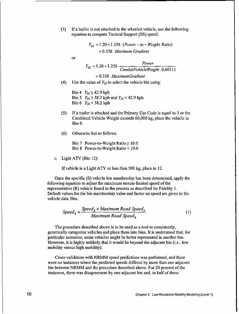
(3) If a trailer is not attached to the wheeled vehicle, use the followingequation to compute Tactical Support (SS) speed:

Yss = 1.20 +1.258. (Power - to - Weight Ratio)

+ 0.338. Maximum Gradient

orYss = 1.20 + 1.258. Power

Combat Vehicle Weight -0.00111

+ 0.338 -MaximumGradient(4) Use the value of Yss to select the vehicle bin using:

Bin 4 Yss > 42.9 kphBin5 Yss >38.2kph and Yss<42.9kphBin 6 Yss < 38.2 kph

(5) If a trailer is attached and the Primary Use Code is equal to 3 or theCombined Vehicle Weight exceeds 60,000 kg, place the vehicle inBin 9.

(6) Otherwise bin as follows:

Bin 7 Power-to-Weight Ratio ? 10.0Bin 8 Power-to-Weight Ratio < 10.0

c. Light ATV (Bin 12):

If vehicle is a Light ATV or less than 500 kg, place in 12.

Once the specific (S) vehicle bin membership has been determined, apply thefollowing equation to adjust the maximum terrain-limited speed of therepresentative (R) vehicle found in the process as described for Fidelity 1.Default values for the bin membership value and factor on speed are given in thevehicle data files.

Speeds = SpeedR x Maximum Road Speeds (1)Maximum Road SpeedR

The procedure described above is to be used as a tool to consistently,generically categorize vehicles and place them into bins. It is understood that, forparticular scenarios, some vehicles might be better represented in another bin.However, it is highly unlikely that it would be beyond the adjacent bin (i.e., lowmobility versus high mobility).

Cross-validation with NRMM speed predictions was performed, and therewere no instances where the predicted speeds differed by more than one adjacentbin between NRMM and the procedure described above. For 20 percent of theinstances, there was disagreement by one adjacent bin and, in half of those


instances, the categorization was near the edges of adjoining bins (Baylot andGates 2002).

Output

Maximum terrain-limited speed as an output will be used to govern whether acommanded speed is achievable or not. A routing service outside this model willdetermine the heading and position of the ground vehicle.

Data tables

An example of the terrain data and NRMM speed predictions contained inthe various input files is given in Table 2.2. The files are divided by climate zone

Table 2.2File InformationTitle: NRMMII Predictions Mapped to MLU CodesClimate Zone: 2Bin: High-Mobility TrackedGround Off-RoadCondition dry Speed for the given slopelpitch in percent (mph)visobs 1 -40 -30 -20 -10 0 10 20 30 40mlu 1 0.0 0.0 13.2 36.7 26.9 0.0 0.0 0.0 0.0mlu 2 0.0 0.0 13.2 36.7 26.9 0.0 0.0 0.0 0.0mlu 3 40.0 40.0 40.0 40.0 12.3 6.0 3.9 1.9 0.0... _ __ __ ... _ .. I. .. .. ..... ...... ...

mlu 256 0.0 0.0 0.0 0.0 100.0 0.0 0.0 0.0 0.0

Condition wetvisobs Imlu 1 0.0 0.0 13.2 36.7 26.9 0.0 0.0 0.0 0.0mlu 2 0.0 0.0 13.2 36.7 26.9 0.0 0.0 0.0 0.0

mlu 3 38.1 40.0 40.0 40.0 11.6 5.0 0.0 0.0 0.0

... __ ... ... .. .. .. ... .. .. .. ..mlu 256 0.0 0.0 0.0 0.0 0.0 0.0 0.0 0.0 0.0

Condition snowvisobs I

mlu 1 0.0 30.7 40.0 40.0 40.0 9.3 4.9 0.0 0.0mlu 2 0.0 30.7 40.0 40.0 40.0 9.3 4.9 0.0 0.0mlu 3 40.0 40.0 40.0 40.0 23.7 7.6 4.6 3.0 0.0... ... ... ... ... ... ... ... ... ... ...

mlu 256 0.0 0.0 0.0 0.0 0.0 0.0 0.0 0.0 0.0

Ground road Speed for the given slopelpitch in percent (mph)Condition dry -15 -12 -8 -4 0 4 8 12 15vis 1 27.7 30.0 30.0 30.0 26.6 14.6 0.0 0.0 0.0mlu 726 27.7 30.0 30.0 30.0 26.6 14.6 0.0 0.0 0.0mlu 727 30.0 30.0 30.0 23.6 12.3 8.7 6.8 5.5 4.8mlu 728 ... ... ... ... ... ... ... ... ...

S30.0 30.0 30.0 30.0 23.5 12.3 1 8.8 6.81 5.8

Note: filename: dryclimates_.xml


and subdivided by condition. The reasoning is that it is unlikely that a computer-generated forces simulation (CGF) like OneSAF will simulate a scenarioinvolving more than one climate zone or soil condition, thus, saving computermemory resources. However, this does not preclude additional climatic zone/ soilconditions from being used. Locations of climate zones as 1-deg grids are givenin the STNDMob file climatezones.txt. A utility function is provided fortranslation in STNDMob. The range and meaning of index values are given inTable 2.3.

Table 2.3Definition of Index ValuesIndex Range of Values ReferenceClimate Zone Dry climates (2), humid mesothermal (3), See Appendix A

humid microthermal (4), undifferentiatedhighland (6)

Condition Dry, wet, snow See Appendix ABin 1-12 See Table 1 and Appendix AGround Cross-country, road See Appendix A,visobs 1-16 See Appendix Avis 1-4 See Appendix Amlu 1 - 256 (cross-country) See Appendix A and Appendix B

726 - 749 (road)slope/pitch -40, -30, -20, -10, 0, 10, 20, 30, 40 (cross- See Appendix A

country)-15, -12,_-8, -4, 0,4, 8,_12,15_(road)

Vehicle data

The following tables present the characterization data for the High-MobilityTracked representative vehicle and two other members of this bin. Vehicle IDvalues are arbitrary with values I to 99 reserved for representative bins. For anexample, see Table 2.4.

Table 2.4Vehicle InformationTitle Vehicle Data FileDate-Time of Creation 1112512002Developer USAERDCCertifier PendingVehicle Name MIA1 AMX 30 LeClerc T-80Vehicle ID 1 100 103Representative Bin 1 1 1Speed Factor 1.0 0.9 0.97Gross Weight (kg) 54545 36000 42500On Road Speed Max (kph) 72 65 70Swimming Speed Max (kph) 0 0 0Fording Speed Max (kph) 8 8 8Amphibious Capable 0 0 0Maximum Gradient 60 60 63Engine Power (hp) 1500 793 1213Type (tracked, wheeled) 1 1 1Primary Use 5 5 5Towing Trailer (Y/N) 0 0 0Note: vehiclelDmap.xml


Example Output

Representative vehicles and preset terrain (Level 1, Fidelity 1)

For the most part, the input data indexes to a given NRMM representativevehicle speed prediction. The exception is that linear interpolation is performedon the speed prediction given two adjacent slopes on the index. Table 2.5provides an example for a high-mobility tracked vehicle.

Table 2.5Predictions for High Mobility Tracked Vehicle

Input Output

Soil Visibility/ STGJ Code Slope SpeedClimate Zone Wetness Obstacles MLU % mph

2 Dry 1 270( 19) 0 26.9

2 Dry 1 270 (19) 10 02 Dry 1 270(19) -10 30.0

2 Dry 16 270(19) 0 02 Wet 1 313 (37) 0 11.62 Wet 1 313 (37) 10 5.02 Wet 1 313 (37) 5 8.3_

1 Interpolated from 0- and 10-percent slopes for NRMM predictions.

Specific vehicles and preset terrain (Fidelity 2)

Level 1, Fidelity 2, uses the representative vehicle to serve effectively asthe basis of the speed prediction for a specific vehicle. The ratio of the specificvehicle's maximum road speed and the representative vehicle's maximum roadspeed serves as a factor for the speed as given for Fidelity 1. Table 2.6 providesan example for a T-80 tank as represented by a high-mobility tracked vehicle(MIAI).

Table 2.6Predictions for a T-80 Tank

Input OutputSoil Visibility/ STGJ Code Slope Speed

Climate Zone Wetness Obstacles MLU % mph2 Dry 1 270(19) 0 26.22 Dry 1 270 (19) 10 02 Dry 1 270 (19) -10 29.22 Dry 16 270(19) 0 02 Wet 1 313 (37) 0 11.32 Wet 1 313 (37) 10 4.92 Wet I 313_375 8.1'

'Interpolated from 0- and 10-percent slopes for NRMM predictions.Note: Max speed for MIAl = 72 kph; max speed for T-80 = 70 kph.


3 Medium-ResolutionMobility Modeling (Level 2)

Medium-resolution or Level 2 mobility has two degrees of fidelity. These areenumerated as 3 and 4. The fidelity as described for Degree 3 is much morecomplex than Fidelity Degree 1 and 2 (from Level 1) because of the variability ofthe terrain state and characteristic attributes of the given representative vehicle.Fidelity Degree 4 is described in exactly the same manner as Degree 3, with theexception that a specific vehicle is chosen over a representative vehicle.

Fidelity Degree 4 is an improvement over the Close Combat Tactical TrainerSemi-Automated Forces (CCTT-SAF) as CCTT-SAF uses only representativevehicles (U.S. Army 1996a, b). Furthermore, this capability will allow modelssuch as computer-generated forces to serve better as an analytical tool todistinguish mobility performance between specific vehicles or vehicle designs.

Input Data

Terrain

For this degree of fidelity specific vehicles are not modeled, and theirmobility performance is dictated strictly by their representative vehicle. Theterrain data attribution is generally mapped to the corresponding OneSAFEnvironmental Data Model label given inside parentheses.

a. soilUSCSType (SoilType), number.

b. soilStrengthCone_40 (SoilCone_IndexQBMeasurement to 40 cm).

c. frozenWater Type (FrozenWater Type).

d surfaceType (TerrainRouteType).

e. surfaceCondition (SurfaceSlippery).

f surfaceRoughness (Terrainroughness rootmean_square).

14 Chapter 3 Medium-Resolution Mobility Modeling (Level 2)

g. snowDepth (Snow-Depth).

h. snowDensity (Snow-Density).

i. vegetationTreeDiameter (MeanStemDiameter).

j. vegetationAverageStemSpacing(MeanStemSpacingQBStemDiameter).

k. obstacleHeight (HeightAboveSurfaceLevel).

L. obstacleWidth (Width).

m. obstacleApproachAngle (Surface-Slope).

n. obstacleMaterialType (Primary_Material_Type).

o. obstacleMu (ObstacleTractionCoefficient).

p. radiusCurvature (computed from array of segment nodes, not in EDM).

Vehicle

Description attributions for vehicle data are as follows:

a. Configuration

(1) TractionElement _Type (Track or Wheeled)

(2) TrailerAttached

(3) PlowBladeCapable

(4) Primary _Use (truck, amphibious (or similar design) combatvehicle, heavy equipment transporter, other)

b. DimensionalData

(1) GrossVehicleWeight, kg

(2) Units (Independent units: powered or unpowered)

(3) Unit-Length, in.

(4) Maximum _UnitWidth, in.

(5) MinimumUnit _GroundClearance, in.

(6) MaximumPushBarForce, lb

Chapter 3 Medium-Resolution Mobility Modeling (Level 2) 15

(7) EnginePower, hp

(8) RotatingMassFactor, none

(9) CenterOf Gravity, in.

(10) Tipping Angle, rad

(11) AxleWidth, in.

(12) AvgTireCorneringStiffness, deg

(13) AssemblyWeight, N

(14) CenterToCenterTreadWidth, m

(15) TrackGroundLength, m

(16) NumTires, none

c. Speed-Boundaries

(1) SpeedBoundaries, kph

(2) MaximumRoadSpeed, kph

(3) Fording, kph

(4) Swimming, kph

(5) RideComfort, rms and kph

(6) Shock, g/kph

d ObstacleManeuver

(1) Maximum_VerticalObstacle, m

(2) MaximumArticulationAngle, deg

(3) MaximumFordingDepth, m

(4) MaximumGradient, %

(5) ObstacleGeometry versusOverRideForceMatrix, in. and rad

(6) ObstacleGeometryInducedShockversusSpeedMatrix, in./sec

e. SurfaceTractionData (for each Power/Throttle Setting, same as CCTT-SAF)


(1) Dry conditions

(2) Slippery conditions

(3) Winter conditions (snow and ice)

f BrakingData (for five positions)

(1) Dry conditions

(2) Slippery conditions

(3) Winter conditions (snow and ice)

g. MotionAttribution

(1) Vehicle-Pitch (SurfaceSlope or pitch)

(2) ThrottlePosition (100, 80, 60, 40, 20 percent of maximum throttle)

NOTE: More detail and example data are given in Appendix C.

Process

Description

This level resembles the mobility implementation in OTB-JVB, OTB-MMBL, JointSAF 5.7, and CCTT-SAF (U.S. Army 1996a, b; Mason et al. 2001;JPSD Program Office 2002). The implementation considers the physicalinteraction between forces and the effects on the velocity of the vehicle.Additionally, behavioral factors are addressed.

Physical model

Tractive forces. The traction-speed relation for the vehicle is determinedfrom the vehicle's power train and traction element characteristics and the currentsoil type, strength, and surface condition. Various vehicle mobility impedimentsin the form of resistances are determined. The sum of all impeding resistances iscompared with the traction-speed relation. If the traction exceeds the resistanceforce sum, excess vehicle traction is available and a suitable running speed isdetermined. Otherwise, if resisting forces are greater than available traction, avehicle immobilization (maximum speed = 0) condition results.

NRMM incorporates a representation of a vehicle's power train to estimatethe vehicle's theoretical power in the form of a maximum available-traction-versus-drive-element-speed relation. This model requires performance andconfiguration characteristics of the power train including the engine output


torque versus speed (rpm) relation curve, torque converter characteristics (ifapplicable), transmission gear ratios and efficiencies, and final drive information.Optionally, the theoretical traction-speed relation can be determined throughphysical testing and provided as an input to NRMM.

The traction-slip relation and soil motion resistance is derived for the givensoil type, soil strength, and surface condition. NRMM uses this information toproduce a traction-speed relation for the specific vehicle/terrain combination. Thefundamental soil relations in NRMM use an empirical system that relates vehicleperformance to soil strength in terms of rating cone index (RCI) for cohesivesoils (clays, silts, and wet sands) or the (semi-empirical) numeric system relatingperformance to soil cone index (CI) for noncohesive soils (dry sands).Performance on winter surfaces (ice, snow, packed snow, snow over soft soil) isbased on empirical algorithms within the NRMM.

In Figure 3.1, a comparison of tractive force required by a typical vehicle andmaximum tractive force made available to the drive train is given (U.S. Army1996a). NRMM, and thus STNDMob, uses an approximation of the tractive-force available to estimate the performance of the vehicle. The differencebetween these forces is the force available for accelerating the vehicle. Lowerthrottle settings would yield a smaller difference.

Tractive Force

.- Tractive - force required

-- - Tractive - force availablew/gearing

First Gear ....... Tractive - maximum forcet-•. available

•/ NSecond Gear

I•"•..•. High Gear

Speed

Figure 3.1. Comparison of tractive force required and tractive force available


The traction coefficient can relate directly to the vehicle's ability to climbslopes, override vegetation, and negotiate obstacles. Soil strength is defined forthe subsurface and is indicated by Rating Cone Index (RCI) on the axis. Thetraction coefficient is defined as the required tractive force divided by vehicleweight.

fT FT (2)WV

where

FT - required tractive force {func of TP, Vt, ST, SS, SL, SN, SD, Sd}

Wv gross vehicle weight

TP throttle position

V = translatory speed

ST soil type, USCS, nondimensional

SS soil strength, RCI

SL slipperiness, nondimensional

SN snow type

SD = snow depth

Sd snow density

Figure 3.2 illustrates the variation of tractive force required to achieve agiven speed. These relationships will change as a function of soil types and soilstrength.

To reduce the complexity and data volume for lower resolution models,NRMM can produce traction coefficient tables that vary as a function of soiltype, soil strength, slipperiness, and throttle position. The tractive forcecoefficient is based on a rectangular hyperbola in Equation 3 and is fitted to thetraction-speed relation using a modified least-squares curve-fit algorithm.Additionally, maximum and minimum traction coefficients are provided torealistically bound the extents of the hyperbolic equation values. This level offidelity is sufficient for a CGF.

f = ffTMIN> b° -b 2 < fTMX (3)V -b,

where

frmAx = normalized maximum tractive force, coefficient

fTMlN = normalized minimum tractive force, coefficient


Traction Performance of a Tracked Vehicle (GRIZZLY)USCS Soil Types: SM, SM/SC, GM, GM/GC Operating on Slippery Surfaces

0.1

03

02

Speed, MPH

S; Soil Strength, RCI

Figure 3.2. Traction-required relationships under slippery conditions for thegiven soil group for a vehicle as a function of soil strength andvehicle speed

FTMAX = maximum tractive force {func of TP, Vt, ST, SS, SL, SN,SD, Sd}

FTMIN = minimum tractive force {func of TP, Vt, ST, SS, SL, SN,SD, Sd}

b0,b1,b 2 = hyperbolic curve-fit coefficients for tractive force

and the normalized tractive force can be computed at a given speed, V, and noacceleration.

Resistance forces. The forces considered here encompass resistances due tosoil interaction/surface friction, air, snow, water, and gravity. Adhesion tosurfaces is greatly affected by the contact area of the tire (sensitive to inflationpressure) or track, surface material, and conditions of the surface. Thus, theresulting rolling resistance force, FR, can widely vary. This is illustrated inTable 3.1.


Table 3.1Coefficient of Rolling Resistance

Vehicle Type Concrete Hard Soil Sand

Heavy truck 0.012 0.06 0.25

Tracked vehicle 0.0381 0.0451

Note: Computed by dividing rolling resistance, FR, by vehicle weight W (Taborek 1957).1 Field observed values used for on-road conditions by NRMM.

There are empirical methods for computing rolling resistance as a function ofsoil type, road type, snow, ice, vehicle traction element (wheel/track), etc. Thesemethods are found in pages 58-67 of the NRMM User's Guide with specificupdates to snow/ice found in the appendix of the NRMM Addendum.' NRMMholds the value of FR as a constant although it tends to increase as the speed ofthe vehicle increases (Taborek 1957). Since cross-country speeds are typically agreat deal less than on-road speeds, this is a good assumption and suitable for aCGF.

The drag forces caused by water and air are modeled in NRMM. Empiricalformulas for computing the hydrodynamic drag and aerodynamic drag resistanceforces are found in the NRMM User's Guide (Ahlvin and Haley 1992). Theseforces can be substantial and limiting. For purposes of a CGF, hydrodynamicforces will not be considered since ground vehicles are expected to be in wateronly a small fraction of the operation duration. Instead, a maximum speed forfording and swimming is provided for the vehicle when crossing bodies of water.

As was shown for the required tractive forces, NRMM has a method forreducing the complexity for models such as a CGF. It does this by adding theaerodynamic resistance coefficient to the tractive force required. This isacceptable as they both are a function of vehicle speed. Thus, as implemented inSTNDMob, the values for tractive-force-required is a summation of the surfaceresistance and the aerodynamic resistance (at sea level).

Braking forces. The NRMM defines total braking as the sum of the motionresistance of braked and unbraked traction elements and the forces acting on thebraking mechanisms for each traction element. Furthermore, NRMM considersthe weight of the vehicle as supported by braked, unbraked, powered, andunpowered traction elements. STNDMod differs in that it does not consider theindividual attributes of each traction element when applying the braking force;instead, it uses the net effect on the vehicle. Therefore, STNDMob is dependentupon NRMM to yield the net effect and is sufficient for a CGF. The total brakingforce occurs at the centroid of the vehicle body and is a function of the forceapplied to the braking mechanism, the motion resistance as limited by the terrain,and the power train resistance internal to the vehicle. NRMM does not considerany change in motion resistance that varies with speed. For simplification, the

1 R. B. Ahlvin, "NRMM Edition II, User's Guide Addendum" (in preparation), U.S.

Army Engineer Research and Development Center, Vicksburg, MS.


braking force due to braked traction elements, BF, on a level surface will be

supplied from NRMM.

FE = min(BP. BF, FTMAX) (4)

where

BP = brake setting expressed as a fraction from zero to one

BF = braking force due to braked traction elements {func of ST, SS,SL, SN, SD, Sd}

FTMAx = maximum tractive force {func of ST, SS, SL, SN, SD, Sd)

Sum of longitudinal resistive forces and gravitational effect. Resistiveforces discussed thus far in this section have dealt with forces that impede themovement of the vehicle at the traction element. Their sum and available tractiveforce, F, on a level surface is given as

F = FT + FR + FB (5)

where F is the sum and available tractive force along a level surface, in pounds.

Since these forces act only in the direction of travel, their effect on availabletractive force is diminished by the cosine of the grade, 0, and the force ofgravity, Wy, will vary by the sine of the grade. Thus, on a level surface there is noeffect of gravity, and on a vertical surface the force of gravity is equal to theweight of the vehicle.

Since the field data used by NRMM available for FT, FR, and FE aremeasured only on a level surface and act only along this vector component, theavailable tractive force, FG, must be resolved to the vector component parallel tothe grade. Thus,

FG =FT• cose+FR cosEO+FB• cosO®+WV *sinjn (6)

where E is the slope (pitch, grade).

However, the tractive force-speed relationships used in NRMM and thusSTNDMob are developed strictly for a level surface. Thus,

FG=F (7)cos0

After substitution of FG in Equation 6 and with simplification:

F =FT +FR +FB +Wv -tanE (8)

This relationship is important, as it is the basis for Equation 3. Thisrelationship will be further developed in later sections.


Vegetation and obstacle forces. The NRMM computes vegetation andobstacle interaction effects as external forces acting on the vehicle, typically viainterpolated look-up tables or empirical equations. These forces as modeled byNRMM can act as either a point obstacle or area obstacle. The key distinctionbetween vegetation modeled as an obstacle and other obstacles is that, if thevehicle is powerful enough, it can deform a tree (drive over) and thus override.

The force required to override a tree is referred to as the push-bar-force, FpB.This force occurs at the impact point, hpB, of the vehicle bumper and tree. Theamount of force required to override the tree is given as a function of tree diam-eter, D. The field data used by NRMM for push-bar forces were measured atvarious heights and are valid for heights below 80 in. The empirical formulationis given in Equation 8.

The required push-bar force isF =Cl 40 hPB 3hPB ) (9)

where

c, = conversion factor, lb/in.4

hpB = vehicle bumper/push-bar height above ground, in.

D = tree diameter, in.

If the value of FpB is greater than or equal to the maximum push-bar forceallowed either by vehicle design or driver comfort, the vehicle will not beallowed to override the tree. Equation 9 is useful for calculating the forcerequired to override a single-tree encounter or perhaps an orchard of trees withequal diameters. The NRMM uses another method for computing multiplesimultaneous encounters within a typical forest. This method considers theaverage stem diameter, D of trees within a class of tree stem diameters. There areeight stem diameter classes: >0 cm, >2.5 cm, >6 cm, >10 cm, >14 cm, >18 cm,>22 cm, and >25 cm. These values also are used to set the maximum stemdiameters, DmAx, for each class. The sum of the simultaneously encounteredforces for all stem diameter classes is given in the empirical equation below.

n

FVEG = c 2 ' 12-wd. 100. Zd j Dj3 (10)j=l

where

C2 = conversion factor, lb/in.2

wd = vehicle width, in.

n = number of classes

j = index increment


d = vegetation density for each class, in.2

D = average stem diameter of class, in.

At present, obstacles other than vegetation are assumed to be nondeformable.Thus, the concept of push-bar force does not apply. NRMM uses preprocesseddata from other models such as OBSMOD or VEHDYN to determine whetherthe geometry of a vehicle can traverse an obstacle without the geometry of anobstacle interfering with the crossing (Creighton 1986). The obstacle geometry isassumed to be a trapezoid defined by the approach (ingress/egress) angle, height,and width. The interaction between geometries is ultimately reduced to theclearance of a vehicle over the obstacle. A zero or negative value of clearance inthe data would indicate a "no-go" condition and, thus, the vehicle certainly couldnot traverse the obstacle without deformation.

For the case when the minimum clearance is greater than zero, a linear,multidimensional interpolation is performed on the generalized trapezoidalshapes found in the given data to be the closest in shape to the obstacle inquestion, in order to compute the maximum required tractive force, FOBMAX,

required to traverse the obstacle and the average resistance force, FOB. Theaverage resistance force is used for considerations of simultaneous encounters ofother obstacles such as trees, whereby their sum of forces required to overridemay cause a "no-go" or speed-reduction circumstance. STNDMob does not yetconsider this complex obstacle case.

Plowing forces. The STNDMob uses a data table to interpolate the plowingforce resistance, Fp, from a multidimensional array of plow depths, soilstrengths, and soil groups (NRMM specific). These tables are provided for a full-width plow with tines, a track-width plow with tines, a full-width blade/rake withno tines, and a track-width blade/rake with no tines. In the final sum of forcesequation, this force is treated simply as an additional resistance.

Resistance forces and speed limits associated with steering. It is beyondthe scope of this effort to provide a complete review of the tire/terrain/vehicledynamics involved in a turning maneuver. However, two significant textbooksthat address this are Milliken and Milliken (1995) and Gillespie (1992).Additionally, as the Army Standard Mobility Model and the basis for STNDMobAPI, the NRMM documentation also provides insight and applicable algorithms(Ahlvin and Haley 1992). The STNDMob API was not intended to model allaspects of vehicle dynamics, but to capture the effects of vehicle performanceand terrain interaction to the extent that, in a CGF application, vehicle behaviorsneed only be represented to the point where an analyst or user does not observeunrealistic behavior.

Table 3.2 indicates which terrain effects can be easily modeling in twodimensions and within a CGF. Studying the issue from another perspective,speeds on a curve or in a turning maneuver can be controlled primarily bytraction (slide/spin or overshoot) or by the vehicle suspension (rollover).


Table 3.2Description of Effects to Be Modeled During a Turning ManeuverEffect I Description/Example/Issue important parameters1

Limit speed on a curve "Spin out," rollover Lateral force, super-elevation,weight distribution,wheelbase, radius ofcurvature or planned path,current heading, tirecornering stiffness,suspension

Steering angle and yaw How fast can the vehicle react to a Slip angle, velocity, corneringvelocity change in steering angle/or react to stiffness

change in heading orderLimit/reduce speed due Given that a future maneuver Route plan, radius ofto maneuver anticipation requires a lower speed, some curvature, current speed

method is required to determine thedeceleration as that maneuverlocation is approached

Induced resistance in Longitudinal component of cornering Cornering stiffness, radius ofthe longitudinal direction force; give an example of 20 percent curvature, super-elevation

power requirement to overcome force(Milliken and Milliken 1995)

Surface type, grade, and other parameters associated with straight-line movement are assumed.

The rationale, algorithms, and procedures for implementation of turningeffects on vehicle performance in STNDMob API are often described by a frictioncircle diagram, which can be used to portray traction forces in a turningmaneuver (Figure 3.3). The y-axis represents the traction available forlongitudinal motion (in the direction of the current heading), negative valuesindicate braking. The x-axis represents the traction available for changing thecurrent heading (lateral force); positive values are for right-hand turns, andnegative values for left-hand turns. What is important to recognize is that avehicle generally operates within the circle (race car drivers attempt to operate onthe circle) and that the magnitude of the resultant of the traction forces requiredfor forward and lateral motion is

Fresutt -(F1""g2 + Fiaterai2 1/2 (11)

where Flong and Fatert are functions of longitudinal slip, slip angle, and maximumtraction coefficient. (The term coefficient implies that the normal force was usedto normalize the lateral or longitudinal force, i.e., a friction coefficient).


Heading

L ft Turn Rig tt rn

- 0.204 .6

B r B k kin

Figure 3.3. Friction circle, with forces incoefficient form

For on-road analysis, NRMM uses the friction coefficients in Table 3.3.Within STNDMob, dry normal and wet slippery coefficients are implementedand are selected through use of variables found in the EDM (see Input Datasection of this chapter).

Table 3.3On-Road Friction Coefficients Available for Use in NRMMRoad Surface Condition' [ Driving [ Braking

Dry, normal 0.9 0.75Dry, slippery 0.8 0.75Wet, normal 0.7 0.6Wet slippery 0.5 0.45Ice 0.1 0.07

'These descriptions correspond to NRMM scenario names and typical combinations.

Within the NRMM, as previously discussed, a tractive force-speed curve isdeveloped based on non-velocity-dependent forces (soil strength, engine power,slope resistance, etc.), and this curve is then adjusted for speed-dependent forces(e.g., cornering forces, aerodynamic drag). Finally, those effects that produceabsolute speed limits are determined (e.g., absorbed shock, rollover) to adjust thespeed. The minimum of the speed limits and the tractive force-speed curve is out-put as the maximum terrain-limited speed for the given conditions. In otherwords, the NRMM produces estimates of both velocity- and non-velocity-dependent resistances to motion, along with absolute speed limits, and combinesthese with potential vehicle performance to estimate a maximum vehicle-capablespeed for a given set of terrain conditions.

Much of the following is extracted directly from Ahlvin and Haley (1992)and the NRMM source code. The resulting effects-associated algorithms andapplications associated with vehicle performance during a turn are described


below. For cornering and side slope effects, NRMM considers three terrain

conditions:

a. Roads (superhighway, primary and secondary roads).

b. Trails (deformable soil surfaces).

c. Cross-country (deformable soil surfaces).

Additionally, wheeled and tracked vehicles or vehicles that have both wheel andtrack elements are treated differently. For roads and trails, radius of curvature andsuper-elevation are inputs; for cross-country, a radius of curvature is calculatedbased on vegetation stem spacing (for each vegetation class). The assumption isthat the only reason to turn on cross-country terrain is related to vegetationavoidance. Cornering forces are generally velocity dependent and are used toadjust the tractive-force-speed curve, while stability effects are represented asspeed limits. Calculations are generally made on a traction element (axle) basisand summed over traction elements, differentiating between powered andnonpowered elements when necessary.

Vehicle cornering speed limits and resistances on trails. Longitudinalresistance during cornering induced by lateral forces is summed over the wheelelements (axles) of wheeled or partially wheeled vehicles (e.g., half-tracks). Thelongitudinal cornering resistance (F,,) is originally from Smith (1970):

Fc = y(V 2m/R )2 ;r/[180 nfc (u/lO.75)] (12)

where

V = tangential velocity of the vehicle

m = mass of the vehicle supported by an element

R = radius of curvature to the center of gravity of the vehicle

n = number of tires on the element

f = empirical correlation coefficient (0.96)

c = average cornering stiffness (lbf/deg)

p = maximum friction coefficient for current terrain

Interestingly, Smith (1970) suggests this as an approximation with [t as anempirical constant of 0.2 based on limited testing. It may be possible to derive asimilar equation based on an expanded bicycle model, but the approach taken forEquation 12 has yet to be implemented.

Super-elevation correction factor for tire cornering resistance. Althoughnot fully implemented yet, a correction (multiplier) to the cornering resistance forsuper-elevation is given as


FE = (1 - gR®/V2)2 (13)

where

e = road super-elevation angle, rad

g = acceleration of gravity, ft/sec2

Tandem axle alignment drag force on a level surface. This applies to allwheel assembles identified as tandem. Thus, the summation over the number oftandem assemblies is given by

FTc = (uY WT cos (grade) Lr)/2R (14)

where

/u = traction coefficient (u/ or Tf as appropriate)

WT = weight on i h tandem axle, lb

grade = current slope (vehicle pitch) angle, rad

LT = center-to-center spacing of tandem wheels on ith tandemaxle, in.

R = radius of curvature of road, in.

Tipping and sliding on trails (cross country). The sliding equation fortrails is the same as for on-road, using the traction coefficient based on soil typeand strength, or snow type, and the slope (vehicle roll direction) for super-elevation. Tipping off-road is concerned with both static rollover, rollover downhill, and dynamic rollover (primarily down hill, as in a turn with negative super-elevation). The equation is much more elaborate than the on-road algorithm, andrequires significant amounts of information regarding the suspension. Thedocumentation does not state why this is the case, although it is possible that it isdue to the steep off-road slopes and increased deflections. The requiredsimultaneous equations and their solution is much too complex to include inSTNDMob API, thus static analysis is used.

Tracked vehicles on roads and trails. Lateral forces associated withsteering tracked suspension elements (NRMM subroutineIV6R2) are computedas a resistance. This resistance is given by the Merritt equation (Merritt 1946 orRay 1979) in terms of the vehicle width-to-length ratio (Merrit 1946, Ray 1979,Peters 1995).

For an individual traction element (or track "set") I, the "Merritt constant" iscalculated as

Mki= ao + a, Ai + a 2 Ai2 a3 Ai 3 (15)

where

Ai = center-to-center distance between tracks on ground


ao = 1.0624

a, = -0.6999

a2 = 0.051848

a3 = 0.05488

thus, a "radius factor" (Ki) is derived as

Ki= Mki(ao-a1R + a2R2 + a3R

3) (16)

where

R = radius of curvature of road, ft

ao = 1.18

a, = -9.0895 x 10-3

a2 = 3.779 x 10-5

a3 = -6.70476 x 10-8

Furthermore, where the summation is over the total number of tracked assembliesand

p = surface traction coefficient

Wi = weight on the ith tracked assembly (lb)

the turning resistance is then calculated by

FCT = PYXKiWi (17)

Additionally, the radius of curvature should be less then 309 ft for trackedvehicles because Ki can become negative and thus

K, = MAX(Ki, 0.0) (18)

On-road cornering speed limits and resistances. Speed limited by sliding(NRMM subroutine IV 1 OR) is the speed at which the centrifugal force of thevehicle in the curve is balanced by the contact friction force (Figure 3.4), asfollows:

VsLIDING = [Rg(pu+ tan 0)/(1 - u tanO)]0 2 (19)


Figure 3.4. Free-body diagram

Speed limited by tipping. Tipping is obtained from the equationexpressing the equilibrium of moments around the outer tire (or track) and thepavement contact point. The forces involved are the centrifugal force and theweight of the vehicle. Thus, the tipping velocity, VTlp, can be determined by

VTip = [Rg(W,,,,, + Ycg tan (O)/(Ycg - Wt..,. tan E)]/ 2 (20)

where

R = radius of curvature, ft

g = gravity, ft/sec2

Wtmx = controlling lateral distance to the center of gravity (the smallestof 1/2 the distance between wheel centers over all axles)

Y = height of center of gravity, corrected for tire inflation, in.

e = road super-elevation angle, rad

The AASHO maximum speeds are taken from relations derived from criteriaused by the American Association of State Highway Officials (1966). (AASHOis now called the American Association of State Highway and TransportationOfficials, AASHTO.) There are two implementations within the NRMM. Theoriginal is an interpolation of Table 3.4, shown plotted in Figure 3.5. Thesevalues are based on conservative traction forces. The second implementationwas developed from changes to this rationale and is explained in Ahlvin andHaley (1992). This revised algorithm was implemented in NRMM version 2.2.0and is referenced as the function "ASHATO2." Primarily, this approach nowestimates a lateral friction coefficient based on the AASHTO ratio and NRMM-predicted longitudinal force. The following equations are solved iteratively, bycomparing the input radius of curvature to that produced by Equation 21:


Table 3.4AASHO Maximum Speeds Used in NRMM_ _ __

Radius of Superhighways Primary SecondaryTrismpCurvature, ft mph Roads, mph Roads, mph

5730 100 100 70 55

1910 70 70 60 49

1146 60 60 58 44

819 54 54 50 42

637 48 48 43 39

458 41 41 36 34

327 34 34 31 29

229 29 29 26 23

164 25 25 23 19

115 19 19 19 14

82 13 13 13 10

Speed, mph

100

90 -

80

•.,• ° .o.- . .... -.... -.........60 . ..........

50 -40 -- "--. . Super-highways &

30 47"Primary roads30 - ---.-.-.-.-.. Secondary roads

10• - Trails

00 1000 2000 3000 4000 5000 6000

Radius of curvature, ft

Figure 3.5. Plot of maximum vehicle speeds for the AASHO algorithm in NRMM

R 14.95(e+f) (21)

where

V = maximum safe speed, mph

f = friction coefficient, none

e = tan 0


This empirical equation will yield the maximum safe speed V, for a given radiusR (ft). The AASHTO friction coefficient, As, is a function of speed, V, wherefAsis the AASHTO friction coefficient (none). Thus,

fAS = 0.678 - 0.00468 V (22)

A straight-line fit of the AASHTO coefficient of longitudinal friction for drypavements was obtained from a variety of stopping tests,fAL, versus speed, where

JAL is the AASHTO longitudinal friction coefficient (none). Thus,

fAL = 0.670-0.00174 V (23)

The ratio of the side friction to longitudinal friction for a given speed is usedas a factor to convert the actual NRMM-predicted coefficient to an equivalentside friction. The following equation is used to determine the side frictioncoefficient for curvature speed predictions (fps) as a function of speed andNRMM-predicted longitudinal friction coefficient (fpL):

f PS= f fPL (24)f AL

where

fps = side friction coefficient, none

fpL = NRMM-computed longitudinal friction coefficient, none

The next relation determines the margin of "safety factor" to be included.This is related to the AASHTO-recommended design coefficient (fA) by settingthe safety factor, S, to a value of 1.0 and to the maximum side coefficient (fps) bysetting it to a value of 0.0 or anywhere in between as a compromise. Thefollowing equation yields the final friction coefficient:

f = (A -fA) S + fPs (25)

where

fA = AASHTO road design coefficient, none

S = compromising factor from physical and AASHTO design limit,none

To facilitate obtaining the AASHTO-recommended side friction coefficients(JA), the following curve was obtained by fitting the data points to a hyperbola.For speeds <20 mph, the value for 20 mph (0.21) is used. The followingequation yields the side friction coefficient:


1

fA= V >:20(3.264+0.07648V) (26)

= 0.21, V<20

wherefAL is the recommended side friction coefficient (none).

In the implementation, the maximum AASHTO-recommended coefficient offriction is not allowed to exceed the model prediction for longitudinal traction.The scheme used for hard surfaces was arbitrarily applied to the soft soils (trails)and snow-covered roads and trails. The AASHTO reference provides very littleinformation concerning the friction coefficients for wet pavements. Theimplications are that the longitudinal friction coefficients are usually much lessthan for dry pavements. The AASHTO design criterion used is the same since itis assumed to apply to an arbitrarily poor condition. Therefore, the same frictionreduction scheme used for dry pavements was assumed to apply to wetpavements. Note that, for the NRMM implementation, the AASHTO informationregarding coefficients of friction on dry pavements is used only to determine theratio of longitudinal to lateral friction; the actual longitudinal friction is obtainedfrom other relations in the NRMM model.

Figure 3.6 illustrates this algorithm, which compares the "bicycle" modelapproximation with the NRMM ASHATO2 algorithm for two high-mobilitymultipurpose wheeled vehicles (HMMWVs) in a steady-state turn of radius132 m. Based on this analysis, the STNDMob implementation uses a value of0.5 for S.

The final on-road curvature speed limit is the minimum of VsLID, VTIp, and theASHATO2 speed. This is later compared with other terrain-limited speeds toarrive at the maximum predicted speed of the vehicle in question.

Sum of longitudinal forces. The physical forces discussed thus far act on thecentroid of the vehicle. The previous sections dealt with resistance forces actingat the traction element, gravitational forces, and forces external to the vehicle.Since the weight of obstacles is seldom known, any gravitational effect fromthese external forces is neglected. However, the gravitational force induced bythe weight of an attached plow is accounted for in Equation 28. Building uponthe previously described Equation 6, the available tractive force, F, is

FG =(FT +F, +FB).cosO+(Wv +Wp).sinO (27)

+ (FPBXOrFVG ) + (FOBAXorFOB )+ FP

where Wp is the weight of attached plow/rake and, with simplification using

Equation 7,

F=(FT +FR +FB)+(Wv +Wp).tanO

+ [(FPB orFVEG ) + (FOB orFOBMAX)] (28)cosO


Steering angle, deg.

12 I NRMM

S=O.0

10 I I Neutral steerIIangle

NRMM - Bicycle model8S=0.5 / understeer grad = 4.5

A//II-Characteristic velocity,understeer grad = 4.5

NRMM ........ Bicycle model,

S = 1.0 understeer grad = -0.34

4 I I -- Critical speed,understeer grad = -0.34

2 I .1 .......................0 I

10 24 30 40 50 60 70 80

"-2Velocity, M/s

Figure 3.6. Comparison of the "bicycle" model (HMMWVs with understeer gradients of 4.5 and -0.34)with the NRMM ASHATO2 algorithm

Maximum terrain-limited speed, longitudinal. The maximum terrain-limited speed can be computed by solving Equation 3 for V, substituting it withVTL, substituting fT with F/(W y+Wp) andfTmIN andfTMx. The resultingEquation 29 is developed. This is the concluding equation found in STNDMobfor computing maximum terrain-limited speed. Where VTL is the maximumterrain-limited speed (mph),

VTL= +b b2, FTMIN F FTMAx (29)

4 C


Behavioral Model

Vehicle behavior should not be limited to what "should be done," but ratherwhat the driver, be it human or autonomous, directs the vehicle to do. The phys-ical model should report to the behavioral model that sliding or tipping is aboutto occur, so that the decision can be made in the next time period whether tochange the settings for throttle, steering, and braking. Some of these speedboundaries were introduced in the previous sections regarding tipping andsliding. It is a source of debate whether AASHTO-recommended settings are aphysical or behavioral boundary.

Without debate, a vehicle predicted speed due to visibility conditions isdriver dependent. Visibility inputs are expected to come from three sources. Theatmosphere will provide an attribute-defining visibility as correlated toobscurants such as fog or smoke near the ground. The terrain will provideattribution-defining visibility as controlled by the vegetation. There will be aline-of-sight based on elevation contours. The minimum of these three attributeswill be the input for mobility modeling purposes.

Speed constraints on a vehicle due to a driver's recognition distance (visibil-ity) are based on stopping distance. The standard method for measuring visibilityin vegetation is based on a 1-ft star placed just above the ground and at a heightof 5 ft above the ground. The driver must recognize at least two points on thestar. For on-road purposes, the visibility is based on the recognition distance for asmall object in the road. For the purposes of a CGF we can assume that visibilityand driver recognition distances are equal and neglect the effect of height aboveground.

As discussed in a previous section, braking force is conditional to the brakingposition as dictated by the driver in Equation 4. An expansion of this relationshipis

FB = min (DCLMAX . W, BP . BF, FTmx) (30)

where DCLMAXis the maximum braking acceleration the driver will accept,expressed as a factor on acceleration of gravity (g = 32.2 ft/sec 2).

Additionally, if the distance, D, is greater than the distance required to avoidimpact or miss a way-point, the FB should be increased by increasing BP and therequired deceleration to come to a complete stop at the desired point. Thus,

a F- (31)W

where a is the required deceleration (ft/sec2).

The maximum speed or velocity permitted in order to stop within or at thespecified distance is given by


Vv-s =a -t + t+ 2 Da (32)

where

Vvjs = required speed, ft/sec

t = time between recognition and application of brakes, sec

D = recognition distance and distance required to stop, ft

In consideration of the amount of absorbed-power due to surface roughnessthe driver/equipment is willing to endure over a given amount of time, a "ride"speed, VR1DE, is set. This limit is usually about 8 hr for 6 W absorbed power bythe driver/equipment. STNDMob provides this as a look-up table as a functionof surface roughness and speed.

Similarly, STNDMob considers the amount of shock that a driver orequipment is willing to sustain when encountering an obstacle. The impact of thevehicle's traction element and the obstacle varies and usually increases as theheight of the obstacle increases. Thus, the impact speed, VoBs, will decrease asthe height of the obstacle increases and will eventually become zero at a givenheight. STNDMob provides this as a look-up table as a function of obstacleheight and speed.

For safe tire operation, STNDMob provides "limits" on speed, VTIrE, due totire design and suspension of the vehicle. This is the maximum safe tire speed,VTIRE, and is the speed limit for which a tire of a particular design and deflectioncan endure the buildup of heat within the tire for a sustained hour. Neither ofthese speed limits is suitable for a CGF unless the speed limit is given as afunction of sustained time.

After consideration of both terrain-limited speed and driver-behavior-limitedspeed, the predicted speed is

V =min (VTL,VVIsVRDE,5VoBS,VTIRE) (33)

Example Output

Representative vehicles and variable terrain (Level 2, Fidelity 3)

Table 3.5 provides an example for a high-mobility tracked vehicle. AnM1AI is used as the representative vehicle.


Table 3.5Example of High-Mobility Tracked Vehicle

Soil Vegetation Surface

Soil Type Strength Surface Obstacle Avg Spacing IRoughness Slope Speed(USCS) (RCIICI) I Condition Height, in. Jft (RMS), in. 1% Imph

SM 300 Dry 0 0 0 0 39.5SM 300 Dry 0 0 0 10 17.5SM 300 Dry 0 0 0 40 4.1SM 50 Dry 0 0 0 0 22.0SM 50 Dry 0 0 0 10 12.3SM 50 Dry 0 0 0 40 2.8

SM 50 Slippery 0 0 0 40 1.5SM 100 Snow 0 0 0 0 33.3SM 100 Snow 0 0 0 20 7.3SM 300 Dry 24 0 0 0 25.3SM 300 Dry 0 20 0 0 27.8SM 300 Dry 0 0 3 0 13.3SP 300 Dry 0 0 0 0 40.7SP 300 Dry 0 0 0 10 18.8SP 300 2y 0 0 0 40 0.0

Note: All terrain attributes as defined in the input data section are not given in this example.______

Specific vehicles and variable terrain (Level 2, Fidelity 4)

Level 2, Fidelity 3, uses the representative vehicle to serve effectively as asubstitute for the speed prediction of a specific vehicle, whereas Fidelity 4 usesthe actual vehicle data file for a specific vehicle. Table 3.6 provides an examplefor a T-72 tank.

Table 3.6Example of T-72 TankSoil Soil Obstacle Vegetation SurfaceType Strength Surface Height Avg Roughness Slope Speed(USCS) (RCIICl) Condition in. Spacing, ft (RMS), in. % mph

SM 300 Dry 0 0 0 0 31.5SM 300 Dry 0 0 0 10 16.0SM 300 Dry 0 0 0 40 2.9SM 50 Dry 0 0 0 0 19.7SM 50 Dry 0 0 0 10 11.1SM 50 Dry 0 0 0 40 1.7SM 50 Slippery 0 0 0 40 1.5SM 100 Snow 0 0 0 0 27.5SM 100 Snow 0 0 0 20 6.3SM 300 Dry 24 0 0 0 0.0SM 300 Dry 0 20 0 0 20.4SM 300 Dry 0 0 3 0 12.0SP 300 Dry 0 0 0 0 35.5SP 300 Dry 0 0 0 10 16.8SP 300 Dry 0 0 0 40 0.0

Note: All terrain attributes as defined in the input data section are not given in this example.


4 Summary

Mobility is a key performance parameter that must be represented accuratelyand consistently within and across military M&S to produce valid interactionsand support conclusions for decision-makers regarding system performance,force design, tactics, and doctrine. The detail required to represent ground vehiclemobility varies with the study level (engineering level versus tactical versusoperational) with the goal of the simulation (e.g., training versus analysis). Modelimplementation within a simulation impacts the consistency with representationsin other simulations. These further impact consistencies between unit locations,selected routes, traverse times, and discrimination in platform performance. Amodel-centric approach to mobility implementation tends to preclude generalizedapplicability to other simulations within or across levels of fidelity.

Current mobility implementation in M&S is largely tailored for specificmodels, leading to inconsistency between models. Cross-model consistencyrefers to agreement between representations in M&S of differing resolutions orlevels of detail. For example, the mobility implementation in one simulation issuch that vehicles are grouped into four classes for performance calculations:high and low mobility wheeled and tracked vehicles. Furthermore, vehicle speedwithin a class is calculated based on nine slope values and one of four visibilitylevels. In the second simulation vehicles are mapped into nine bins, and speedcalculations incorporate a continuous function of slope and visibility levels.Thus, the same vehicle will likely exhibit different speed performance under thesame conditions in the two simulations.

To assist the decision-makers in analysis, acquisition, and training issues, itis necessary to provide and promote consistency between models to be used inthe analysis. The developing M&S systems plan to employ the NRMM, theAMSO standard for ground vehicle mobility (e.g., OneSAF OperationalRequirements Document, COMBATxxl Functional Requirements Document).Without a holistic approach, actual implementations could produceinconsistencies and invalid behaviors for cross-model analysis andinteroperability. Furthermore, this approach should enable NRMM enhancementsand upgrades to be readily implemented as the STNDMob matures toaccommodate advanced system issues (e.g., robotics and urban operations use).

The development of the STNDMob API suite is a definitive step in achievingthe goal of cross-model consistency for ground vehicle mobility representation.The STNDMob API is a generalized, platform-independent implementation

38 Chapter 4 Summary

derived from NRMM to facilitate the standardized integration of entity-levelmobility constraints into Department of Defense (DoD) simulations. A validationstudy of Level 1 was conducted by the AMSAA and has been documented(Fischer 2004). A comparison of NRMM and STNDMob Level 2 is given inAppendix D so that a user can understand the limitations of the derivation.

Ease of integration was accomplished with the assistance of softwareenhancements such as Java and XML. The use of the API in COMBATxxI showsits viability as a DoD product. Within the STNDMob API design, there areimplementations that account for various levels of fidelity associated with theresolution of the input and output parameters. The development of generic APIsor object models will facilitate integration of the model into future simulations.Moreover, this approach will allow for upgrading the model with minimalreengineering of simulation links. The results of this research will savedevelopers time and money and will promote implementation of model andalgorithm improvements.

Chapter 4 Summary 39

References

Ahlvin, R. B., and Haley, P. W. (1992). "NATO Reference Mobility Model,Edition II; NRMM user's guide," Technical Report GL-92-19, U.S. ArmyEngineer Research and Development Center, Vicksburg, MS.

American Association of State Highway Officials (AASHO). (1966), "A policyon geometric design of rural highways, 1965,"Washington, DC.

Baylot, E. A., and Gates, B. Q. (2002). "Procedure for categorizing groundvehicles," ERDC/GSL TR-02-21, U.S. Army Engineer Research andDevelopment Center, Vicksburg, MS.

Baylot, E. A., and Goerger, N. C. (2003). "Ground vehicle mobility steady state:Low resolution (Level 1), " KEMA070007, U.S. Army Materiel SystemsAnalysis Activity, Aberdeen Proving Ground, MD.

Baylot, E. A., Gates, B. Q., Goerger, N. C., and Goerger, S. R. (2003). "Gettingone of the basics right for distributed simulations: A mobility service/serverfor the present and future," 03F-SIW-123, Simulation InteroperabilityWorkshop. Simulation Interoperability Standards Organization, Orlando, FL.

Birkel, P. (1999). "The Terrain Common Data Model (TCDM): A joint effort forJSIMS, STOW, and JWARS," 8th-CGF-004, Lockheed Martin,Burlington, MA.

Bullock, C. D. (1994). "Methodology for the development of inferencealgorithms for worldwide application of interim terrain data to the NRMM,"Technical Report GL-94-37, U.S. Army Engineer Research and Develop-ment Center, Vicksburg, MS.

Creighton, D. C. (1986). "Revised vehicle dynamics module: User's guide forcomputer program VEHDYN II," Technical Report SL-86-9, U.S. ArmyEngineer Research and Development Center, Vicksburg, MS.

Fisher, W. (2004). "Validation of the standard mobility applicationprogrammers' interface; Vol 1, Fiedlity I and 2," Technical Report No. 754,U.S. Army Materiel Systems Analysis Activity, Aberdeen Proving Ground,MD.

40 References

Gillespie, T. D. (1992), Fundamentals of vehicle dynamics, ISBN 1-56091-199-9. SAE International, Warrendale, PA.

Joint Precision Strike Demonstration (JPSD) Program Office. (2002). "Systemdetailed description for the Joint Virtual Battlespace (JVB)," FortBelvoir, VA.

Mason, G. L., Ahlvin, R. B., and Green, J. G. (2001). "Short-term operationalforecasts of trafficability," ERDC/GSL TR-01-22, U.S. Army EngineerResearch and Development Center, Vicksburg, MS.

McKinley, G. B., Deliman, N. C., and Falls, T. C. (2001). "A standards basedmovement and infrastructure aggregation methodology for mobilityrepresentation in modeling and simulations," ERDC/GSL TR-0 1-21, U.S.Army Engineer Research and Development Center, Vicksburg, MS.

Merrit, H. E. (1946). "The evolution of a tank transmission," Proceedings,Institution of Mechanical Engineers 154, 412. Institution of MechanicalEngineers, London, UK.

Milliken, W. F., and Milliken, D. L. (1995). Race car vehicle dynamics.ISBN 1-56091-526-9. SAE International, Warrendale, PA.

Peters, J. (1995), "Analysis of soil-track interaction for computer programTVSTEER," Technical Report GL-95-6, U.S. Army Engineer Research andDevelopment Center, Vicksburg, MS.

Ray, J. R. (1979). "Investigation of the factors involved in steering tracklayingvehicles," Technical Report No. 10969 (AD871157), U.S. Army Tank-Automotive Command, Warren, MI.

Smith, G. L. (1970). "Commercial vehicle performance and fuel economy,"SP-355, The Society of Automotive Engineers, New York, NY.

Taborek, J. J. (1957). "Mechanics of vehicles," Parts 1-13. Machine Design,Cleveland, OH.

U.S. Army. (1995). "Warfighter's Simulation 2000 software descriptiondocument," Program Executive Office Simulation Training Instrumentation(PEO-STRI), Orlando, FL.

S(1 996a). "CCTT dynamic behavior, design synthesis report," PEO-STRI, Orlando, FL.

___ (1996b). "Compendium of CCTT algorithms, data, data structuresand generic system mappings," PEO-STRI, Orlando, FL.

_ (2000). "OneSAF objective system environmental data model,"Version 1.0, PEO-STRI, Orlando, FL.

References 41

U.S. Army. (2002). "OneSAF operational requirements document," Version 1.1,PEO-STRI, Orlando, FL.

42 References

Appendix AGeneration of Mobility SpeedPredictions

The U.S. Army Engineer Research and Development Center (ERDC) hasdeveloped a set of standard databases for use in representing vehicle mobilityacross major M&S programs. The Program Executive Office SimulationTraining Instrumentation for the Warfare Simulation 2000 (WARSIM) sponsoredthe development of the off-road mobility requirements. Resulting mobilitydatabases have been implemented in JWARS, OneSAF, and COMBATxxI in aneffort to promote reuse and interoperability among M&S programs.

NRMM terrain databases were built for four major regions (climate zones)using WARSIM-specific soil, vegetation, slopes, visibilities, and obstaclerequirements and inference algorithms developed by the ERDC Geotechnical andStructures Laboratory (GSL). Mobility predictions were made for dry, wet, andsnow scenarios using representative vehicles from each mobility class.

Regions

The Worldwide Climate Zones as produced by G. T. Trewartha and pub-lished in Goode's WorldAtlas (16th edition, Rand McNally and Company, 1983)are listed in Table Al. Terrain databases have been produced for all majorclimate zones excluding the Tropical Rainy and the Polar Climates. The Desert,the Humid Subtropical, and the Humid Continental-Warm Summer subclimatezones were selected to represent the Dry, the Humid Mesothermal, and theHumid Microthermal climate zones, respectively.

Scenarios

ERDC-GSL was sponsored by WARSIM to provide mobility data for dry-normal and wet-slippery scenarios. In support of COMBATxxl and JWARSmobility efforts, snow data were also generated.

Appendix A Generation of Mobility Speed Predictions Al

Table AlWorldwide Climate Zones - Subclimate ZonesA- Tropical Rainy Climates

Tropical Rainforest, Tropical Savanna

B. Dry ClimatesSteppe, Desert

C. Humid Mesothermal ClimatesMediterranean or Dry Summer Subtropical, Humid Subtropical, Marine West Coast

D. Humid Microthermal ClimatesHumid Continental, Warm Summer, Humid Continental, Cool Summer, Sub-Arctic

E. Polar ClimatesTundra, Ice Caps

F. Undifferentiated HighlandsUndifferentiated Highlands

Vehicles

Vehicles were bundled into 12 groups based on mobility and configuration,and representative vehicles were selected per group. Table A2 lists the vehiclebundles and representative vehicle for each bundle.

Table A2Vehicle Bundles and Representative VehiclesVehicle Bundle Representative Vehicle

High-Mobility Tracked MIA1Medium-Mobility Tracked M270-MLRSLow-Mobility Tracked M60-AVLBHigh- Mobility Wheeled M1084Medium-Mobility Wheeled M985Low-Mobility Wheeled M917High-Mobility Wheeled w/trailer M1084-M1095Medium-Mobility Wheeled w/trailer M985-M989Low-Mobility Wheeled w/trailer M911-M747Amphibious Combat Vehicle Tracked M113A2Amphibious Combat Vehicle Wheeled LAV25Light ATV (unmanned) Kawasaki ATV

MLU Code Development

There are 255 Mobility Look-Up (MLU) off-road and 24 MLU on-roadtrafficability codes that map to the WARSIM Terrain Common Data Model(TCDM) surface trafficability groups JSIMS (STGJ) (Birkel 1999).' These off-road codes are based on the exhaustive combinations of 15 Interim Terrain Data(ITD) vegetation coverage codes and 17 ITD soil types (Table A3). The on-roadcodes are based on road type and surface material combinations (Table A4).(Note: Not every vegetation and soil type combination exists in the real world.Furthermore, codes exist only in particular regions of the world. However, for

See References at the conclusion of the main text.

A2 Appendix A Generation of Mobility Speed Predictions

implementation and balance purposes, all 255 indices are used in each climatezone.)

ETable A3

Specified Vegetation and Soil Types _ ______

[Index Vegetation J Soil

1 Wetlands GW2 Bareground GP3 Dry Agriculture GM4 Wet Agriculture GC5 Orchard/Plantation SW6 Vineyard/Hops SP7 Grassland/Pasture/Meadow SM8 Brushland/Scrub SC9 Bamboo/Cane ML

10 Deciduous Forest CL11 Coniferous Forest OL12 Mixed Forest CH13 Forest Clearing MH14 Swamp OH15 Mangrove PT16 _________________ Evaporites (CLM L)17 Rock Crops (Rock)

Table A4Road DescriptionsCart Track or US-Trail UK-Trail/Footpath: GW

Cart Track or US-Trail UK-Trail/Footpath: GP

Cart Track or US-Trail UK-Trail/Footpath: GM

Cart Track or US-Trail UK-Trail/Footpath: GC

Cart Track or US-Trail UK-Trail/Footpath: SW

Cart Track or US-Trail UK-Trail/Footpath: SP

Cart Track or US-Trail UK-Trail/Footpath: SM

Cart Track or US-Trail UK-Trail/Footpath: SC

Cart Track or US-Trail UK-Trail/Footp•ath: ML

Cart Track or US-Trail UK-Trail/Footp3ath: CL

Cart Track or US-Trail UK-Trail/Footp•ath: OL

Cart Track or US-Trail UK-Trail/Footp3ath: CH

Cart Track or US-Trail UK-Trail/Footp•ath: MH

Cart Track or US-Trail UK-Trail/Footp3ath: OH

Cart Track or US-Trail UK-Trail/Footp•ath: PT

Cart Track or US-Trail UK-Trail/Footpath: Evaporites

Road: Hard/Paved

Road: Loose/Paved

Road: Loose/Light

Road: Corduroy

Road: Grass/Sod (Soft)

Road: Natural

Road: Permanent

Road: Temporary

NRMM Terrain Development

NRMM terrain format 7 was used to create the terrain files. This format wasselected because it allows both road and spatial data in the same terrain file and itis in a free-field format (space or comma delimited). Both on-road and off-roadterrain require the following characteristics: surface condition and depth, soiltype, soil strengths for 0- to 6-in. and 6- to 12-in. layers, depth to bedrock, slope,surface roughness and visibility. Additional characteristics include road type andsurface, super-elevation angle (in degrees), and radius of curvature (feet) for on-road terrain and obstacle geometry and vegetation spacing for off-road terrain(Bullock 1994).

WARSIM specified values for off-road slopes and for visibility and obstaclespacing distances. ERDC-GSL inference routines were used to define region-specific soil strengths, surface roughness, and vegetation spacing. ERDC subjectmatter experts provided number values for road type, soil/surface type, surfacecondition and depth, depth to bedrock, super-elevation angle, and radius ofcurvature. Separate terrain files were created by climate zone, scenario, roadtype, and visibility-obstacle spacing categories.

Specified Data

Visibility

Situational visibility is a function of the surface and slope on which thevehicle is operating, the distance the driver can see, and the vehicle's maximumbraking ability. Visibility is related to the maximum speed the vehicle can traveland still be brought to a stop under maximum braking within the visibilitydistance. Based on work with WARSIM developers, the visibility distanceswere set at 25, 50, 100, 300 ft (where 300 ft is equivalent to an unlimitedvisibility condition). Table A5 provides the rationale for these values. Table A6further extends the rationale for visibility of off-road terrain based upon land use,seasons, and climate zone.

Battlefield clutter or obstacle spacing

Based on work with WARSIM developers, it was determined that all obsta-cles would be 8 ft long, 8 ft wide, and 45 in. tall with a 90-deg approach angle.Obstacles would be simulated at spacings of 20, 25, 30, and 150 ft (where 150 ftis equivalent to a no-clutter condition). These settings virtually ensured that novehicle could maneuver over the obstacles and that distinctions in maneuver-ability between larger and smaller vehicles would be apparent. See Table A7 forvisibility settings when obstacles are combined.


Table A5Visibility for On-Road ConditionsVisibility (vis, Distanceroad) (ft) Meaning

1 300 Unlimited, distance spacing of vehicles, no precipitation, daytimelighting, headlights at night, no obscurants, good contrast.

Somewhat limited, distant spacing of vehicles, light precipitation,2 100 daytime lighting, headlights at night, obscurants or blackout

w/vision enhancement devices, fair contrast.Limited, close spacing of vehicles, heavy precipitation/fog, low

3 50 solar/lunar illumination, heavy obscurants w/vision enhancementdevices, poor contrast.Very limited, close spacing of vehicles, no solar/lunar illumination,

4 25 heavy obscurants and/or blackout w/no enhanced vision devices,very poor contrast.

SSee the references listed below for additional information on these topics:

- Convoy spacing [McKinley et al. 2001]- Computing transmissivity due to obscurants ["Combined obscuration model for battlefield

induced contaminants (COMBIC)," U.S. Army Research Laboratory, Adelphi, MD]- Computing recognition distance due to contrast as a function of transmissivity ["Target

Acquisition Model (TARGAC)," U.S. Army Research Laboratory, Adelphi, MD, and "NightVision Goggle Operations (NOWS)," Phillips Laboratory, Geophysics Directorate, HanscomAFB, Maine]

Table A6Seasonal Visibility Based on Land Use Type

Climate ZoneHumid Humid Undifferentiated

Dry Mesothermal Microthermal HighlandsLand Use Type W SISFs F w sIsSlF WI S SIFWetland 3 3 4 3 2 3 3 2 2 3 3 2 2 2 2 2Dry crop 1 4 4 1 1 3 4 1 1 3 3 1 1 4 4 1Shifting crop 1 4 4 1 1 3 4 1 1 3 3 1 1 4 4 1Terraced crop 1 4 4 1 1 3 4 2 1 3 3 1 1 4 4 1Rice paddy 1 3 4 1 1 3 3 1 1 3 3 1 1 3 4 1Agricult. w/scat trees 1 4 4 1 1 3 3 1 1 3 3 1 1 4 4 1Orchard 2 3 3 22 1 2 3 2 2 2 22 2 3 3 2Vineyard 2 3 3 2 2 3 3 2 2 3 3 2 2 3 3 2Pasture/meadow 1 2 2 1 1 2 2 1 1 2 2 1 1 2 2 1Grassland 1 3 4 1 1 2 2 1 1 2 2 12 2 1Grasslandw/scat 1 3 4 2 1 2 2 1 1 2 2 1 1 2 2 1treesScrub 3 4 4 2 2 3 4 2 2 2 2 2 2 3 3 2Bamboo 4 4 4 4 4 4 4 4 4 4 4 4 4 4 4 4Deciduous forest 2 3 3 3 2 3 3 2 2 3 3 3 2 3 3 2Coniferous forest 2 3 3 3 2 3 3 3 2 3 3 3 2 3 3 2Mixed forest 3 3 3 3 2 3 3 3 2 3 3 3 2 3 3 2Palm 2 3 4 2 2 2 3 2 2 2 2 2j 2 2 3 2Mangrove 4 4 4 4 4 4 4 4 3 4 4 3 4 4 4Forest clearing 1 2 2 1 1 1 1 1 1 1 1 1 2 2 1Bareground 1 1 111 11 11 1 1 11 1 1 1

W - Winter Jan-Mar, S - Spring Apr-Jun, S - Summer Jul-Sep, F - Fall Oct-Dec.Visibility 1 (300 ft), 2 (100 ft), 3 (50 ft), 4 (25 ft).More climate zones are given in Bullock (1994), but must be mapped to the 4 visibility distances.

Appendix A Generation of Mobility Speed Predictions A5

Table A7Visibility and Obstacle CombinationsVisibility andOba Obstacle

Combinations Obstacle(visobs, cross- Distance Spacingcountry) ft ft Meaning

1 300 150 See vis meaning plus uncluttered, no vegetation,bareground.

2 100 150 See vis meaning plus uncluttered, sparsevegetation or vegetation in winter.

3 50 150 See vis meaning plus uncluttered, vegetation inspring to fall.

4 25 150 See vis meaning plus uncluttered, densevegetation.

5 300 30 See vis meaning, cluttered due to urban orindustrial area damage, concentration of damagedvehicles, cratering, rubble, rock outcrops, somevegetation.

6 100 30 "7 50 308 25 309 300 25 Same as above and redundant.

10 100 2511 50 2512 25 2513 300 20 See vis meaning, severely cluttered due to heavy

urban or industrial area damage, denseconcentration of damaged vehicles, cratering,rubble, rock outcrops, dense vegetation.

14 100 2015 50 20 116 25 20

Note: See Tables A4 and A5.

Slopes

Off-road. WARSIM predetermined slopes for off-road terrain were set as-40, -30, -20, -10, 0, 10, 20, 30, and 40 percent. These values correspond withthe CCTT values.

On-road. By road design, major roads will not have slopes greater than30 or 40 percent. According to research accomplished in concurrence with theJWARS mobility effort, maximum slopes would be 15 percent (McKinley et al.2001). Based on input from subject matter experts, it was determined that trailcategories could be set as equivalent to off-road slope categories (0, 10, 20, 30,40 percent), but maximum slopes on superhighways, primary, and secondaryroads should be limited to 15 percent. Thus, slopes were assigned for these roadsas 0, 4, 8, 12, 15, -4, -8, -12, and -15 percent (McKinley et al. 2001).


Surface condition

Surface condition was set to 1 for normal conditions and 2 for slipperyconditions.

Surface depth

Surface depth equals 0 when scenario is dry or wet. Surface depth equalsdepth of snow or ice for winter conditions.

Depth to bedrock

Depth to bedrock was arbitrarily set to 99 in. NRMM ignores any valuelarger than 12.

Distance

Distance per terrain unit was set to 0.05 mile (264 ft).

Super-elevation and radius of curvature

ERDC specified super-elevation angles (EANG) and radius of curvaturevalues (RADC) for roads are shown in Table A8.

Table A8Super-Elevation (EANG) and Radius of Curvature (RADC) DataRoad Type J IROAD I EANGý deg I RADC, ftOff-road 0 n/a n/aSuperhighway 1 0.12 5730Primary road 2 0.12 5730Secondary road 3 0.06 5730Trail 4 0.00 5730

Road and road surface material types

ERDC specified road type (IROAD) and surface material type for roads andcart tracks, as shown in Table A9.


Table A9Road and Road Surface Material Types

SurfaceRoad Description IROAD Type/

I MaterialCart Track or US-Trail UK-Trail/Footpath: GW 4 GWCart Track or US-Trail UK-Trail/Footpath: GP 4 GPCart Track or US-Trail UK-Trail/Footpath: GM 4 GMCart Track or US-Trail UK-Trail/Footpath: GC 4 GCCart Track or US-Trail UK-Trail/Footpath: SW 4 SWCart Track or US-Trail UK-Trail/Footpath: SP 4 SPCart Track or US-Trail UK-Trail/Footpath: SM 4 SMCart Track or US-Trail UK-Trail/Footpath: SC 4 SCCart Track or US-Trail UK-Trail/Footpath: ML 4 MLCart Track or US-Trail UK-Trail/Footpath: CL 4 CLCart Track or US-Trail UK-Trail/Footpath: OL 4 OLCart Track or US-Trail UK-Trail/Footpath: CH 4 CHCart Track or US-Trail UK-Trail/Footpath: MH 4 MHCart Track or US-Trail UK-Trail/Footpath: OH 4 OHCart Track or US-Trail UK-Trail/Footpath: PT 4 PTCart Track or US-Trail UK-Trail/Footpath: Evaporites 4 CLMLRoad: Hard/Paved 2 PAVERoad: Loose/Paved 3 MLRoad: Loose/Light 4 MLRoad: Corduroy 1 PAVERoad: Grass/Sod (Soft) 4 SMRoad: Natural 4 SMRoad: Permanent 1 PAVERoad: Temporary 4 SM

Inference Data

Soil strength

Soil strength, or Relative Cone Index (RCI), values are given for layers 0-6 in. and 6-12 in., respectively. RCIs are inferred from wetness index, soil type,soil moisture, and region. Soil moisture is determined using soil type, andwetness index is inferred by slope, soil type, vegetation, and region.

a. Wetness indices (Table AIO) are dependent upon climate zone and slope.

Table A10Wetness Index

Wetness Index Description

0 AridI Dry (steep slopes, semiarid regions)

2 Average (well drained)3 Wet (poorly drained, bottomlands)4 Saturated (flooded part of the year)5 Waterlogged (perennially waterlogged)


b. Rules used for assigning the wetness index (WI) are as follows (Bullock1994):

(1) If vegetation = wetlands, swamp, or mangrove, WI = 5.

(2) If vegetation = wet crops, WI = 4.

(3) If vegetation # wetlands, swamp, mangrove, or wet crops, considerthe climate region and slope as given in the following table.

Table AllWetness Indices for Vegetation Not Equal toWetlands, Swamp, Mangrove, or Wet CropsRegion/Slope 10 110 J20 130 J40Desert 2 1 1 1 1

Humid Mesothermal 4 3 3 2 2

Humid Microthermal 4 4 3 2 2

Undiff Highlands 3 2 2 2 2

(4) WI for negative slopes: use those given for positive slopes.

Surface roughness

Surface roughness measurements (RMS) were inferred from vegetation, soiltype, and region. Sources include Table 46 of Bullock (1994) and the XLATEtranslation algorithm that contained some of the tables as referenced. When thetwo differed, Table 46 of Bullock (1994) was used. Table A12 provides thepertinent values.

a. Major versus minor. XLATE contained RMS values for each majorclimate zone but not for the subclimate zones.

b. Bareground Table 46 shows that RMS varies by soil type whenvegetation = bareground. In discussing RMS values for trails, this wouldalso be true.

c. Swamp. No RMS data are given in Table 46 for swamps. In XLATE,swamps were assumed mixed, and RMS data for mixed forests wereassigned to swamps. This was assumed in TVCC-VEG as well.

d. Crops. Dry crops = wet crops.

e. Forests. Coniferous forest = mixed forest = swamp.


Table A12RMS Data Used

Humid Humid F UndiffDesert Mesothermal Microthermal Highlands

Wetland 0.3 1.4 1.4 1.4Bareground - Gravel 0.6 0.6 0.6 1.0Bareground - Sand 0.3 0.6 0.6 1.0Bareground - Clay/Silt 0.6 0.6 0.6 1.4Bareground - Rock 1.8 1.8 1.8 2.2Dry Crops 0.6 0.6 0.6 1.0Orchard/Plantation 0.6 0.6 1.0 1.0Vineyard 0.6 0.6 1.0 1.0Grassland 0.6 0.6 0.6 1.0Brush/Scrub 1.4 1.4 1.4 1.8Bamboo 1.0 1.0 1.0 1.0Deciduous Forest 1.0 1.0 1.4 1.4Coniferous Forest 1.0 1.4 1.4 1.4

Forest Clearing 1.0 1.4 1.8 1.8Mangrove 1.8 1.8 1.8 1.8

Vegetation

Vegetation is necessary only for orchards, forests, and swamps. Bullock(1994) does not include vegetation for swamps. Swamps were assumed mixedtree types. Swamps and mangroves are not different by climate zone, and neitherare orchards. Tables A13-A16 provide the indicated spacings given in units offeet. The value of 328 ft (100 m) is assumed to be the greatest distance that thespacing of vegetation would influence speed.

Table A13Vegetation for Desert _T_6_SS

I Bins ISi S2 IS3 1S4 Is S 5 6 IS7 IS8Dec Forest 1-5 1 3 15 328 328 328 328 328Con Forest 1-5 1 2 25 328 328 328 328 328Mix Forest 1-5 1 2 21 328 328 328 328 328Orchard XLATE 30 30 32 32 34 45 55 60Swamp XLATE 30 30 32 32 34 45 55 60Mangrove XLATE 22 22 22 22 22 28 28 30

Inferred from the ERDC-GSL XLATE algorithm for vegetation spacing and given in feet.


Table A14Vegetation for Humid Mesothermal

I Bins [S1 ]s2 [S3 1S4 IS5 6 S S7 6s80 26-30 9 10 11 12 15 20 31 115Con Forest 26-30 9 10 10 12 14 20 34 248Mix Forest 26-30 9 9 12 15 18 22 28 66

Orchard XLATEi 30 30 32 32 34 45 55 60Swamp XLATE 30 30 32 32 34 45 55 60Mangrove XLATE 22 22 22 22 22 28 28 30


Table A15Vegetation for Humid Microthermal

IBins [IS Is2 [S3 IS4 Is5 S6 IS7 IS8 JDec Forest 11-15 4 5 11 45 328 328 328 328Con Forest 11-15 4 5 11 45 328 328 328 328Mix Forest 11-15 4 5 11 38 195 328 328 328Orchard XLATE' 30 30 32 32 34 45 55 60Swamp XLATE 30 30 32 32 34 45 55 60Mangrove XLATE 22 22 22 22 22 28 28 30

SInferred from the ERDC-GSL XLATE algorithm for vegetation spacing and given in feet.- ____

Table A16Vegetation for Undifferentiated Highlands

IBins [sI IS2 [S3 ]S4 IS S6 Is s7 Is8 1Dec Forest 26-30 9 10 11 12 14 18 27 87Con Forest 26-30 9 9 10 11 14 22 41 328Mix Forest 26-30 9 9 12 14 17 21 28 78Orchard XLATE_ 30 30 32 32 34 45 55 60Swamp XLATE 30 30 32 32 34 45 55 60Mangrove XLATE 22 22 22 22 22 28 28 30


Appendix A Generation of Mobility Speed Predictions All

Appendix BWARSIM Terrain Common DataModel (TCDM) STGJ to MLUMappings

Appendix B WARSIM Terrain Common Data Model (TCDM) STGJ to MLU Mappings B1

STGJ FACC WARSIM

Code Name Feature BMC BUD DMT FTC RST SIC STP VEG MLU

0 Unknown 0

1 Areal Urban: AAO1O Mine AA010 0

2 jreal Urban: AA012 Quarry AA012 0

3 Areal Urban: AA052 Oil / Gas Field; STP: GW AA052 1 18

4 Areal Urban: AA052 Oil / Gas Field; STP: GP AA052 2 19

5 Aeal Urban: AA052 Oil / Gas Field; STP: GM AA052 3 20

6 [eal Urban: AA052 Oil / Gas Field; STP: GC AA052 4 21

7 Aeal Urban: AA052 Oil / Gas Field; STP: SW AA052 5 22

8 Aeal Urban: AA052 Oil / Gas Field; STP: SP AA052 6 23

9 Areal Urban: AA052 Oil / Gas Field; STP: SM AA052 7 24

10 Areal Urban: AA052 Oil / Gas Field; STP: SC AA052 8 25

11 Areal Urban: AA052 Oil / Gas Field; STP: ML AA052 9 26

12 Areal Urban: AA052 Oil / Gas Field; STP: CL AA052 10 27

13 Areal Urban: AA052 Oil / Gas Field; STP: OL AA052 11 28

14 Areal Urban: AA052 Oil / Gas Field; STP: CH AA052 12 29

15 Areal Urban: AA052 Oil / Gas Field; STP: MH AA052 13 30

16 Areal Urban: AA052 Oil / Gas Field; STP: OH AA052 14 31

17 Areal Urban: ACOOO Processing Plant ACOOO 0

18 Areal Urban: AC030 Settling Pond AC030 0

19 Areal Urban: AC040 Oil / Gas Facilities AC040 0

20 Areal Urban: AD010 Power Plant ADOO 0

21 Areal Urban: AD030 Substation AD030 0

22 real Urban: AE010 Fabrication Facility AE010 0

23 Areal Urban: AK030 Amusement Park; STP: GW AK030 1 18

24 Areal Urban: AK030 Amusement Park; STP: GP AK030 2 19

25 Areal Urban: AK030 Amusement Park; STP: GM AK030 3 20

26 real Urban: AK030 Amusement Park; STP: GC AK030 4 21

27 Areal Urban: AK030 Amusement Park; STP: SW AK030 5 22

28 Areal Urban: AK030 Amusement Park; STP: Sp AK030 6 23

29 Areal Urban: AK030 Amusement Park; STP: SM AK030 7 24

30 Areal Urban: AK030 Amusement Park; STP: SC AK030 8 25

31 Areal Urban: AK030 Amusement Park; STP: ML AK030 9 26

32 Areal Urban: AK030 Amusement Park; STP: CL AK030 10 27

33 Areal Urban: AK030 Amusement Park; STP: OL AK030 11 28

34 Areal Urban: AK030 Amusement Park; STP: CH AK030 12 29

35 Areal Urban: AK030 Amusement Park; STP: MH AK030 13 30

36 Areal Urban: AK030 Amusement Park; STP: OH AK030 14 31

37 Areal Urban: AKI 10 Grandstand AK110 0

B2 Appendix B WARSIM Terrain Common Data Model (TCDM) STGJ to MLU Mappings

STGJ FACC WARSIMCode Name Feature BMC BUD DMT FTC RST SIC STP VEG MLU

38 Areal Urban: AK130 US Race Track; STP: GW AK130 1 0

39 Areal Urban: AK130 US Race Track; STP: GP AK130 2 0

40 Areal Urban: AK130 US Race Track; STP: GM AK130 3 0

41 Areal Urban: AK130 US Race Track; STP: GC AK130 4 0

42 Areal Urban: AK130 US Race Track; STP: SW AK130 5 0

43 Areal Urban: AK130 US Race Track; STP: SP AK130 6 0

44 Areal Urban: AK130 US Race Track; STP: SM AK130 7 0

45 Areal Urban: AK130 US Race Track; STP: SC AK130 8 0

46 Areal Urban: AK130 US Race Track; STP: ML AK130 9 0

47 Areal Urban: AK130 US Race Track; STP: CL AK130 10 0

48 Areal Urban: AK130 US Race Track; STP: OL AK130 11 0

49 Areal Urban: AK130 US Race Track; STP: CH AK130 12 0

50 Areal Urban: AK130 US Race Track; STP: MH AK130 13 0

51 Areal Urban: AK130 US Race Track; STP: OH AK130 14 0

52 Areal Urban: AK160 US Stadium / Amphitheater AK160 0

53 Areal Urban: AL015 Building AL015 0

54 Areal Urban: AL020 Built-Up Area AL020 0

55 Areal Urban: ALl05 Settlement; STP: GW ALl05 1 18

56 Areal Urban: ALl05 Settlement; STP: GP ALl05 2 19

57 Areal Urban: ALl05 Settlement; STP: GM ALl05 3 20

58 Areal Urban: ALl05 Settlement; STP: GC ALl05 4 21

59 Areal Urban: ALl 05 Settlement; STP: SW ALl05 5 22

60 Areal Urban: ALl05 Settlement; STP: SP ALl 05 6 23

61 Areal Urban: ALl 05 Settlement; STP: SM AL105 7 24

62 Areal Urban: ALl 05 Settlement; STP: SC ALl05 8 25

63 Areal Urban: ALl05 Settlement; STP: ML ALl05 9 26

64 Areal Urban: ALl05 Settlement; STP: CL ALl05 10 27

65 Areal Urban: AL105 Settlement; STP: OL AL105 11 28

66 Areal Urban: ALl05 Settlement; STP: CH AL105 12 29

67 Areal Urban: ALl05 Settlement; STP: MH AL105 13 30

68 Areal Urban: ALl05 Settlement; STP: OH AL105 14 31

69 Areal Urban: ALI35 Native Settlement; STP: GW AL135 1 18

70 Areal Urban: AL135 Native Settlement; STP: GP AL135 2 19

71 Areal Urban: AL135 Native Settlement; STP: GM AL135 3 20

72 Areal Urban: ALI35 Native Settlement; STP: GC AL135 4 21

73 Areal Urban: AL135 Native Settlement; STP: SW AL135 5 22

74 Areal Urban: ALl 35 Native Settlement; STP: SP AL135 6 23

75 Areal Urban: ALl35 Native Settlement; STP: SM AL135 7 24



76 Areal Urban: ALI 35 Native Settlement; STP: SC AL135 8 25

77 Areal Urban: AL135 Native Settlement; STP: ML AL135 9 26

78 Areal Urban: AL135 Native Settlement; STP: CL AL135 10 27

79 Areal Urban: AL135 Native Settlement; STP: OL AL135 11 28

80 Areal Urban: AL135 Native Settlement; STP: CH AL135 12 29

81 Areal Urban: AL135 Native Settlement; STP: MH AL135 13 30

82 Areal Urban: AL135 Native Settlement; STP: OH AL135 14 31

83 Areal Urban: AL200 Ruins; STP: GW AL200 1 18

84 Areal Urban: AL200 Ruins; STP: GP AL200 2 19

85 Areal Urban: AL200 Ruins; STP: GM AL200 3 20

86 Areal Urban: AL200 Ruins; STP: GC AL200 4 21

87 Areal Urban: AL200 Ruins; STP: SW AL200 5 22

88 Areal Urban: AL200 Ruins; STP: SP AL200 6 23

89 jreal Urban: AL200 Ruins; STP: SM AL200 7 24

90 Areal Urban: AL200 Ruins; STP: SC AL200 8 25

91 Areal Urban: AL200 Ruins; STP: ML AL200 9 26

92 Areal Urban: AL200 Ruins; STP: CL AL200 10 27

93 ýAreal Urban: AL200 Ruins; STP: OL AL200 11 28

94 Areal Urban: AL200 Ruins; STP: CH AL200 12 29

95 Areal Urban: AL200 Ruins; STP: MH AL200 13 30

96 Areal Urban: AL200 Ruins; STP: OH AL200 14 31

97 Areal Urban: AM010 Depot (Storage) AM010 0

98 Areal Urban: AN060 Rail Yard AN060 0

99 Areal Urban: AT050 Communication Building AT050 0

100 Areal Water: Fore Shore; BMC: Clay and Silt BA020 1 0

101 Areal Water: BA020 Fore Shore; BMC: Silty BA020 2 0

102 Areal Water: BA020 Fore Shore; BMC: Sand and BA020 3 0

103 Areal Water: BA020 Fore Shore; BMC: Gravel BA020 4 0104and Cobble BA020 F SrRk A 5

105 Areal Water: BA020 Fore Shore; BMC: Rocks BA020 5 0___and Boulders________

105 Areal Water: BAO20 Fore Shore; BMC: Bedrock BA020 6 0

106 Areal Water: BA020 Fore Shore; BMC: Paved BA020 7 0

107 Areal Water BA020 Fore Shore; BMC: Peat BA020 8 0

108 Areal Water: BA020 Fore Shore; BMC: Sand BA020 9 0over mud ____

109 [Areal Water: BA020 Fore Shore; BMC: Mixed BA020 10 0____ ualities ____

110 Areal Water: BA020 Fore Shore; BMC: Coral BA020 11 0

111 Areal Water: BA020 Fore Shore; BMC: Slash BA020 12 0

112 Areal Water: BA020 Fore Shore; BMC: BA020 13 0Seamount _ _



113 Areal Water BA020 Fore Shore; BMC: Sand BA020 14 0

114 Areal Water: BA040 Water (Except Inland); BA040 1 0BMC: Clay and Silt

115 Areal Water: BA040 Water (Except Inland); BA040 2 0BMC: Silty Sands

116. Areal Water: BA040 Water (Except Inland); BA040 3 0BMC: Sand and Gravel

117 Areal Water: BA040 Water (Except Inland); BA040 4 0BMC: Gravel and Cobble

118 Areal Water: BA040 Water (Except Inland); BA040 5 0BMC: Rocks and Boulders

119 Areal Water: BA040 Water (Except Inland); BA040 6 0BMC: Bedrock

120 Areal Water: BA040 Water (Except Inland); BA040 7 0BMC: Paved

121 Areal Water: BA040 Water (Except Inland); BA040 8 0BMC: Peat

122 Areal Water: BA040 Water (Except Inland); BA040 9 0BMC: Sand over mud

123 Areal Water: BA040 Water (Except Inland); BA040 10 0BMC: Mixed qualities

124 Areal Water: BA040 Water (Except Inland); BA040 11 0BMC: Coral

125 Areal Water: BA040 Water (Except Inland); BA040 12 0BMC: Slash

126 Areal Water: BA040 Water (Except Inland); BA040 13 0BMC: Seamount

127 Areal Water: BA040 Water (Except Inland); BA040 14 0BMC: Sand

128 Areal Water or Hydrography: BHO10 Aqueduct; BH010 1 0BMC: Clay and Silt

129 real Water or Hydrography: BHO10 Aqueduct; BHO10 2 0BMC: Silty Sands

130 Areal Water or Hydrography: BHO10 Aqueduct; BHOIO 3 0BMC: Sand and Gravel

131 Areal Water or Hydrography: BHO10 Aqueduct; BH010 4 0BMC: Gravel and Cobble

132 Areal Water or Hydrography: BHO10 Aqueduct; BHO10 5 0BMC: Rocks and Boulders

133 Areal Water or Hydrography: BH010 Aqueduct; BHO10 6 0BMC: Bedrock

134 Areal Water or Hydrography: BHO10 Aqueduct; BHO10 7 0BMC: Paved

135 Areal Water or Hydrography: BHO1 0 Aqueduct; BH010 8 0BMC: Peat

136 Areal Water or Hydrography: BHO10 Aqueduct; BHO10 9 0BMC: Sand over mud

137 Areal Water or Hydrography: BHO1 0 Aqueduct; 1H010 10 0BMC: Mixed qualities

138 Areal Water or Hydrography: BHO10 Aqueduct; BHOIO 14 0BMC: Sand

139 Areal Water or Hydrography: BH020 Canal; BH020 1 0BMC: Clay and Silt

140 Areal Water or Hydrography: BH020 Canal; BH020 2 0BMC: Silty Sands

141 Areal Water or Hydrography: BH020 Canal; BH020 3 0BMC: Sand and Gravel

142 Areal Water or Hydrography: BH020 Canal; BH020 4 0BMC: Gravel and Cobble

143 real Water or Hydrography: BH020 Canal; BH020 5 0

BMC: Rocks and Boulders



144 Areal Water or Hydrography: BH020 Canal; BH020 6 0BMC: Bedrock

145 Areal Water or Hydrography: BH020 Canal; BH020 7 0BMC: Paved

146 real Water or Hydrography: BH020 Canal; BH020 8 0146 BMC: Peat BH_20_8_

147 [real Water or Hydrography: BH020 Canal; BH020 9 0BMC: Sand over mud

148 Areal Water or Hydrography: BH020 Canal; BH020 10 0BMC: Mixed qualities149 Areal Water or Hydrography: BH020 Canal; BH020 14 0

BMC: Sand

150 Areal Urban: BH040 Filtration Beds BH040 0

151 Areal Water: BHO50 Fish Hatchery BH050 0

152 Areal Water: BHO80 Lake / Pond; BMC: Clay and BHO80 1 0Silt

153 Areal Water: BH080 Lake / Pond; BMC: Silty BHO80 2 0Sands

154 Areal Water: BHO80 Lake / Pond; BMC: Sand BHO80 3 0land Gravel

155 Areal Water: BH080 Lake / Pond; BMC: Gravel BHO80 4 0and Cobble

156 Areal Water: BH080 Lake / Pond; BMC: Rocks BH080 5 0and Boulders

157 Areal Water: BHO80 Lake / Pond; BMC: Bedrock BH080 6 0

158 Areal Water: BH080 Lake / Pond; BMC: Paved BH080 7 0

159 Areal Water: BH080 Lake / Pond; BMC: Peat BH080 8 0

160 Areal Water: BH080 Lake / Pond; BMC: Sand BH080 9 050over mud16 real Water BHO80 Lake / Pond; BMC: Mixed161 iqualities BH080 10 0

162 jreal Water: BHO80 Lake / Pond; BMC: Sand BH080 14 0

163 Areal Vegetation: BH095 Marsh / Swamp; DMT BH095 ? 1 222-= 25, STP: GW

164 Areal Vegetation: BH095 Marsh / Swamp; DMT BH095 ? 2 223-= 25, STP: GP

165 Areal Vegetation: BH095 Marsh / Swamp; DMT BH095 ? 3 224< 25, STP: GM

166 Areal Vegetation: BH095 Marsh / Swamp; DMT BH095 ? 4 225<= 25, STP: GC

167 Areal Vegetation: BH095 Marsh / Swamp; DMT BH095 ? 5 226- 25, STP: SW

168 Areal Vegetation: BH095 Marsh / Swamp; DMT BH095 ? 6 227- 25, STP: SP

169 Areal Vegetation: BH095 Marsh / Swamp; DMT BH095 ? 7 228- 25, STP: SM

Areal Vegetation: BH095 Marsh / Swamp; DMT BH095 ? 8 2291< 25, STP: SC

171 Areal Vegetation: BH095 Marsh / Swamp; DMT BH095 ? 9 230<= 25, STP: ML

172 Areal Vegetation: BH095 Marsh / Swamp; DMT BH095 ? 10 231<= 25, STP: CL

173 Areal Vegetation: BH095 Marsh / Swamp; DMT BH095 ? 11 232< 25, STP: OL

174 Areal Vegetation: BH095 Marsh / Swamp; DMT BH095 ? 12 233<= 25, STP: CH B

175 Areal Vegetation: BH095 Marsh / Swamp; DMT BH095 ? 13 234B6 25, STP: MHA n B 13 234



176 Areal Vegetation: BH095 Marsh / Swamp; DMT BH095 ? 14 235<= 25, STP: OH

177 Areal Vegetation: BH095 Marsh / Swamp; DMT BH095 ? 15 236<= 25, STP: PTAreal Vegetation: BH095 Marsh / Swamp; DMT

178 >= 26, STP: GW BH095 1 222

179 Areal Vegetation: BH095 Marsh / Swamp; DMT BH095 ? 2 223- 26, STP: GP

180 Areal Vegetatidn: BH095 Marsh I Swamp; DMT BH095 ? 3 224>= 26, STP: GM

181 Areal Vegetation: BH095 Marsh / Swamp; DMT BH095 ? 4 225>= 26, STP: GC

182 Areal Vegetation: BH095 Marsh / Swamp; DMT BH095 ? 5 226>= 26, STP: SW

183 Areal Vegetation: BH095 Marsh / Swamp; DMT BH095 ? 6 227>= 26, STP: SP

184 Areal Vegetation: BH095 Marsh / Swamp; DMT BH095 ? 7 228>= 26, STP: SM

185 Areal Vegetation: BH095 Marsh / Swamp; DMT BH095 ? 8 229>= 26, STP: SC

186 Areal Vegetation: BH095 Marsh / Swamp; DMT BH095 ? 9 230> 26, STP: ML

187 Areal Vegetation: BH095 Marsh / Swamp; DMT BH095 ? 10 231>= 26, STP: CL

188 Areal Vegetation: BH095 Marsh / Swamp; DMT BH095 ? 11 232>= 26, STP: OL

189 Areal Vegetation: BH095 Marsh / Swamp; DMT BH095 ? 12 233>= 26, STP: CH

190 Areal Vegetation: BH095 Marsh / Swamp; DMT BH095 ? 13 234>= 26, STP: MH

191 Areal Vegetation: BH095 Marsh I Swamp; DMT BH095 ? 14 235>= 26, STP: OH

192 Areal Vegetation: BH095 Marsh / Swamp; DMT BH095 ? 15 236>= 26, STP: PT

193 Hydrography: BH120 Rapids; BMC: Silty Sands BH120 2 0

194 Hydrography: BH120 Rapids; BMC: Sand and BH120 3 0Gravel

195 Hydrography: BH120 Rapids; BMC: Gravel and BH120 4 0Cobble

196 Hydrography: BH120 Rapids; BMC: Rocks and BH120 5 0Boulders

197 Hydrography: BH120 Rapids; BMC: Bedrock BH120 6 0

198 Hydrography: BH120 Rapids; BMC: Paved BH120 7 0

199 Hydrography: BH120 Rapids; BMC: Mixed BH120 10 0qualities

200 Areal Water: BH130 Reservoir; BMC: Clay and BH130 1 0Silt

201 Areal Water: BH130 Reservoir; BMC: Silty BH130 2 0Sands

202 Areal Water: BH130 Reservoir; BMC: Sand and BH130 3 0Gravel

203 Areal Water: BH130 Reservoir; BMC: Gravel and BH130 4 0Cobble

204 Areal Water: BH130 Reservoir; BMC: Rocks and BH130 5 0Boulders

205 Areal Water: BH130 Reservoir; BMC: Bedrock BH130 6 0

206 Areal Water: BH130 Reservoir; BMC: Paved BH130 7 0

207 Areal Water: BH130 Reservoir; BMC: Peat BH130 8 0



208 Areal Water BH130 Reservoir; BMC: Sand over BH130 9 0mud209 Areal Water: BH130 Reservoir; BMC: Mixed BH130 10 0

.qualities

210 kreal Water: BH130 Reservoir; BMC: Sand BH130 14 0

211 Areal Vegetation: BH135 Rice Field; STP: GW BH135 1 35

212 Areal Vegetation: BH135 Rice Field; STP: GP BH135 2 36

213 Areal Vegetation: BH135 Rice Field; STP: GM BH135 3 37

214 Areal Vegetation: BH135 Rice Field; STP: GC BH135 4 38

215 Areal Vegetation: BH135 Rice Field; STP: SW BH135 5 39

216 Areal Vegetation: BH135 Rice Field; STP: SP BH135 6 40

217 Areal Vegetation: BH135 Rice Field; STP: SM BH135 7 41

218 Areal Vegetation: BH135 Rice Field; STP: SC BH135 8 42

219 Areal Vegetation: BH135 Rice Field; STP: ML BH135 9 43

220 Areal Vegetation: BH135 Rice Field; STP: CL BH135 10 44

221 Areal Vegetation: BH135 Rice Field; STP: OL BH135 11 45

222 Areal Vegetation: BH135 Rice Field; STP: CH BH135 12 46

223 Areal Vegetation: BH135 Rice Field; STP: MH BH135 13 47

224 Areal Vegetation: BH135 Rice Field; STP: OH BH135 14 48

225 Areal Water or Hydrography: BH140 River I BH140 1 0Stream; BMC: Clay and Silt

226 eal Water or Hydrography: BH140 River / BH140 2226 Stream; BMC: Silty Sands 0H140 2_0

227 eal Water or Hydrography: BH140 River / BH140 3 0227 Stream; BMC: Sand and Gravel

228 Areal Water or Hydrography: BH140 River / BH140 4 0Stream; BMC: Gravel and Cobble

229 eal Water or Hydrography: BH140 River / BH140 5 0229 Stream; BMC: Rocks and Boulders

230 real Water or Hydrography: BH140 River / BH140 6 0Stream; BMC: Bedrock

231 Areal Water or Hydrography: BH140 River / BH140 7 0Stream; BMC: Paved

232 Areal Water or Hydrography: BH140 River / BH140 8 0Stream; BMC: Peat

233 Areal Water or Hydrography: BH140 River / BH140 9 0Stream; BMC: Sand over mud

234 Areal Water or Hydrography: BH140 River / BH140 10 0Stream; BMC: Mixed qualities BH4_1_

235 Areal Water or Hydrography: BH140 River / BH140 14 0Stream; BMC: Sand

236 Areal Physiography: BH150 Salt Pan; STP: BH150 18 33Evaporites

237 Areal Urban: BH155 Salt Evaporator; STP: BH155 18 33Evaporites

238 Areal Physiography: BH160 Sebkha; STP: 18 332 Evaporites BH160

239 Areal Water: BH190 Lagoon / Reef Pool; BMC: BH190 1 0Clay and Silt

240 Areal Water: BH190 Lagoon / Reef Pool; BMC: BH190 2 0Silty Sands

241 Areal Water: BH190 Lagoon / Reef Pool; BMC: BH190 3 0Sand and Gravel I II



242 Areal Water: BH190 Lagoon / Reef Pool; BMC: BH190 4 0Gravel and Cobble

243 Areal Water: BH190 Lagoon / Reef Pool; BMC: BH190 5 0Rocks and Boulders

244 Areal Water: BH190 Lagoon / Reef Pool; BMC: BH190 6 0Bedrock

245 Areal Water: BH190 Lagoon / Reef Pool; BMC: BH190 7 0Paved

246 Areal Water: BH190 Lagoon / Reef Pool; BMC: BH190 8 0Peat

247 Areal Water: BH190 Lagoon / Reef Pool; BMC: BH190 9 0Sand over mud

248 Areal Water: BH190 Lagoon / Reef Pool; BMC: BH190 10 0Mixed qualities

249 Areal Water: BH190 Lagoon / Reef Pool; BMC: BH190 11 0Coral

250 Areal Water: BH190 Lagoon / Reef Pool; BMC: BH190 12 0Slash I

251 Areal Water: BH190 Lagoon / Reef Pool; BMC: BH190 14 0Sand

252 Areal Vegetation: BJ110 Tundra; STP: GW, BJ110 1 69 103_ EG: Tundra

253 Areal Vegetation: B1J310 Tundra; STP: GP, VEG: BJ110 2 69 104Tundra

254 real Vegetation: B1Jl10 Tundra; STP: GM, BJ10 3 69 105254 VEG: Tundra BJ110 3_69 _105

255 Areal Vegetation: BJ110 Tundra; STP: GC, VEG: BJ110 4 69 106_ Tundra

256 Areal Vegetation: BJ1 10 Tundra; STP: SW, B1J310 5 69 107VEG: Tundra

257 Areal Vegetation: BJI 10 Tundra; STP: SP, VEG: BJ110 6 69 108Tundra258 Areal Vegetation: BJ1 10 Tundra; STP: SM, VEG: BJ110 7 69 109Tundra

259 Areal Vegetation: BJ110 Tundra; STP: SC, VEG: BJ110 8 69 110Tundra

260 Areal Vegetation: BJ110 Tundra; STP: ML, VEG: BJ110 9 69 '11Tundra

261 Areal Vegetation: B1J310 Tundra; STP: CL, VEG: BJ110 10 69 112Tundra

262 Areal Vegetation: B1J310 Tundra; STP: OL, VEG: BJ110 11 69 113Tundra

263 Areal Vegetation: BJ110 Tundra; STP: CH, VEG: BJ110 12 69 114Tundra264 Areal Vegetation: BJ110 Tundra; STP: MH, BJ110 13 69 115

VEG: Tundra

265 Areal Vegetation: B1J310 Tundra; STP: OH, VEG: BJ110 14 69 116Tundra

266 Areal Vegetation: B1 310 Tundra; STP: PT, VEG: BJ110 15 69 117Tundra

267 Areal Physiography: BJ1OO Snow Field; SIC: BJ100 1 0Snow

268 Areal Physiography: B1J100 Snow Field; SIC: Ice BJ100 2 0

269 Areal Physiography: DA010 Ground Surface DA010 1 18Element; STP: GW

270 Areal Physiography: DA010 Ground Surface DA010 2 19Element; STP: GP

271 Areal Physiography: DA010 Ground Surface DA010 3 20Element; STP: GM

272 Areal Physiography: DA010 Ground Surface DA010 4 21-Element; STP: GC



273 Areal Physiography: DA010 Ground Surface DA010 5 22Element; STP: SW

274 Areal Physiography: DA010 Ground Surface DA010 6 23Element; STP: SP

275 Areal Physiography: DA010 Ground Surface DA010 7 24Element; STP: SM 1

276 Areal Physiography: DA010 Ground Surface DA010 8 25Element; STP: SC

277 Areal Physiography: DA010 Ground Surface DA010 9 26Element; STP: ML

278 Areal Physiography: DA010 Ground Surface DA010 10 27Element; STP: CL

279 Areal Physiography: DA010 Ground Surface DA010 11 28Element; STP: OL

280 Areal Physiography: DA010 Ground Surface DA010 12 29Element; STP: CHAreal Physiography: DA010 Ground Surface DA013

281 Element; STP: MH

282 Areal Physiography: DA010 Ground Surface DA010 14 31Element; STP: OH

283 Areal Physiography: DB160 Rock Strata / Rock DB160 34Formation

284 Areal Physiography: DB170 Sand Dune / Hills; DB170 2 19STP: GP

285 Areal Physiography: DB170 Sand Dune/ Hills; DB170 3 20STP: GM

286 jAreal Physiography: DB170 Sand Dune / Hills; DB170 4 21_ STP: GC

287 Areal Physiography: DB170 Sand Dune / Hills; DB170 5 22STP: SW

288 Areal Physiography: DB170 Sand Dune I Hills; DB170 6 23STP: SP

289 Areal Physiography: DB170 Sand Dune/ Hills; DB170 7 24STP: SM

290 [Areal Physiography: DB170 Sand Dune / Hills; DB170 8 25_ STP: SC

291 Areal Vegetation: EA010 Cropland; FTC: EA010 0 1 35Unknown, STP: GW

292 Areal Vegetation: EA010 Cropland; FTC: Slash EA010 1 1 35and Bum-Shifting cultivation, STP: GW

293 Areal Vegetation: EA010 Cropland; FTC: EA010 2 1 35Permanent field, STP: GW

294 Areal Vegetation: EA010 Cropland; FTC: Ditch EA010 4 1 35Irrigation, STP: GW

295 Areal Vegetation: EA010 Cropland; FTC: EA010 5 1 35_ Grazing, STP: GW

296 Areal Vegetation: EA010 Cropland; FTC: EA010 6 1 35Regular (planting pattern), STP: GW

297 eal Vegetation: EAO10 Cropland; FTC: Linear EA010 7 1 35_ (planting pattern), STP: GW

298 Areal Vegetation: EA010 Cropland; FTC: Not EA010 9 1 3529 pplicable, STP: GW

299 Areal Vegetation: EA010 Cropland; FTC: Type of EA010 98 1 35field Pattem, STP: GW

300 Areal Vegetation: EA010 Cropland; FTC: Other, EA010 999 1 35STP: GW E009913

301 real Vegetation: EA010 Cropland; FTC:301 Unknown, STP: GP EA010 0 2 36

302 jreal Vegetation: EA010 Cropland; FTC: Slash EA010 1 2 36land Bum-Shifting cultivation, STP: GP

303 Keal Vegetation: EA010 Cropland; FTC: EA010 2 2 36permanent field, STP: GP ______

Bl0 Appendix B WARSIM Terrain Common Data Model (TCDM) STGJ to MLU Mappings

STGJ FACC WARSIMCode Name Feature BMC BUD DMT FTC RST SIC STP VEG MLU304 Areal Vegetation: EA010 Cropland; FTC: Ditch EA010 4 2 36

Irrigation, STP: GP305 Areal Vegetation: EA010 Cropland; FTC: EA010 5 2 36

Grazing, STP: GP

306 Areal Vegetation: EA010 Cropland; FTC: EA010 6 2 36Regular (planting pattern), STP: GP

307 Areal Vegetation: EA010 Cropland; FTC: Linear EA010 7 2 36(planting pattern), STP: GP

308 Areal Vegetation: EA010 Cropland; FTC: Not EA010 9 2 36Applicable, STP: GP

309 Areal Vegetation: EA010 Cropland; FTC: Type of EA010 98 2 36field Pattern, STP: GP

310 Areal Vegetation: EA010 Cropland; FTC: Other, EA010 999 2 36STP: GP

311 Areal Vegetation: EA010 Cropland; FTC: EA010 0 3 37Unknown, STP: GM

312 Areal Vegetation: EA010 Cropland; FTC: Slash EA010 1 3 37and Bum-Shifting cultivation, STP: GM

313 Areal Vegetation: EA010 Cropland; FTC: EA010 2 3 37Permanent field, STP: GM

314 Areal Vegetation: EA010 Cropland; FTC: Ditch EA010 4 3 37Irrigation, STP: GM

315 Areal Vegetation: EA010 Cropland; FTC: EA010 5 3 37Grazing, STP: GM

316 Areal Vegetation: EA010 Cropland; FTC: EA010 6 3 37Regular (planting pattern), STP: GM

317 Areal Vegetation: EA010 Cropland; FTC: Linear EA010 7 3 37(planting pattern), STP: GM

318 Areal Vegetation: EA010 Cropland; FTC: Not EA010 9 3 37Applicable, STP: GM

319 Areal Vegetation: EA010 Cropland; FTC: Type of EA010 98 3 37field Pattern, STP: GM

320 Areal Vegetation: EA01 0 Cropland; FTC: Other, EA010 999 3 37STP: GM

321 Areal Vegetation: EA010 Cropland; FTC: EA010 0 4 38Unknown, STP: GC

322 Areal Vegetation: EA010 Cropland; FTC: Slash EA010 1 4 38and Bum-Shifting cultivation, STP: GC

323 Areal Vegetation: EA010 Cropland; FTC: EA010 2 4 38Permanent field, STP: GC

324 Areal Vegetation: EA010 Cropland; FTC: Ditch EA010 4 4 38Irrigation, STP: GC

325 Areal Vegetation: EA010 Cropland; FTC: EA010 5 4 38Grazing, STP: GC

326 Areal Vegetation: EA010 Cropland; FTC: EA010 6 4 38Regular (planting pattern), STP: GC

327 Areal Vegetation: EA010 Cropland; FTC: Linear EA010 7 4 38(planting pattern), STP: GC

328 Areal Vegetation: EA010 Cropland; FTC: Not 9 4 38328 Applicable, STP: GC E00943

329 Areal Vegetation: EA010 Cropland; FTC: Type of EA010 98 4 38field Pattern, STP: GC

330 Areal Vegetation: EA010 Cropland; FTC: Other, EA010 999 4 38STP: GC

331 Areal Vegetation: EA010 Cropland; FTC: EA010 0 5 38Unknown, STP: SW

332 Areal Vegetation: EA010 Cropland; FTC: Slash EA010 1 5 39and Burn-Shifting cultivation, STP: SW

333 Areal Vegetation: EA010 Cropland; FTC: EA010 2 5 39Permanent field, STP: SW

334 Areal Vegetation: EA010 Cropland; FTC: Ditch EA010 4 5 39__Irrigation, STP: SW

Appendix B WARSIM Terrain Common Data Model (TCDM) STGJ to MLU Mappings B1 I

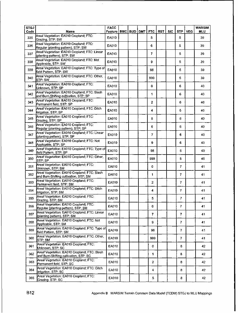
STGJ FACC WARSIMCode Name Feature BMC BUD DMT FTC RST SIC STP VEG MLU335 Areal Vegetation: EA010 Cropland; FTC: EA010 5 5 39

__ Grazing, STP: SW336 Areal Vegetation: EA010 Cropland; FTC: EA010 6 5 39

_ Regular (planting pattern), STP: SW337 t'eal Vegetation: EA010 Cropland; FTC: Linear EA010 7 5 39

1 planting pattern), STP: SW338 Areal Vegetation: EA010 Cropland; FTC: Not EA010 9 5 39

- pplicable, STP: SW

339 Areal Vegetation: EA010 Cropland; FTC: Type of EA010 98 5 39field Pattern, STP: SW

340 Areal Vegetation: EA010 Cropland; FTC: Other, EA010 999 5 39STP: SW 1 9

341 real Vegetation: EA010 Cropland; FTC: EA010 0 6 40341 Unknown, STP: SP

342 lreal Vegetation: EA010 Cropland; FTC: Slash EA010 1 6 40land Bum-Shifting cultivation, STP: SP

343 Areal Vegetation: EA010 Cropland; FTC: EA010 2 6 40_ Permanent field, STP: SP

344 Areal Vegetation: EA010 Cropland; FTC: Ditch EA010 4 6 40Irrigation. STP: SPAreal Vegetation: EA010 Cropland; FTC: EA010 5 6 40

345 Grazing, STP: SP346 Areal Vegetation: EA010 Cropland; FTC: EA010 6 6 40

__ Regular (planting pattern), STP: SP347 Areal Vegetation: EA010 Cropland; FTC: Linear EA010 7 6 40

_ (planting pattern), STP: SP348 Aeal Vegetation: EA010 Cropland; FTC: Not EA010 9 6 40

Applicable, STP: SP349 Areal Vegetation: EAO10 Cropland; FTC: Type of EA010 98 6 40

field Pattern, STP: SP350 Areal Vegetation: EA010 Cropland; FTC: Other, EA010 999 6 40

STP: SP

351 Areal Vegetation: EA010 Cropland; FTC: EA010 0 7 41Unknown, STP: SM352 Areal Vegetation: EA010 Cropland; FTC: Slash EA010 1 7 41

land Bum-Shifting cultivation, STP: SM33 real Vegetation: EA01O Cropland; FTC: E002 7 41

Permanent field, STP: SM354 Areal Vegetation: EA010 Cropland; FTC: Ditch EA010 4 7 41

Irrigation. STP: SM355 Areal Vegetation: EA010 Cropland; FTC: 5 7 41

Grazing, STP: SM EA010 5_7_41

356 Areal Vegetation: EA010 Cropland; FTC: EA010 6 7 41Regular (planting pattern), STP: SM357 Areal Vegetation: EA010 Cropland; FTC: Linear EA010 7 7 41

__ (planting pattern), STP: SM358 Areal Vegetation: EA010 Cropland; FTC: Not EA010 9 7 41

lpplicable, STP: SM359 Areal Vegetation: EA010 Cropland; FTC: Type of EA010 98 7 41

field Pattern, STP: SM360 Areal Vegetation: EA010 Cropland; FTC: Other, EA010 999 7 41

STP: SM

361 Areal Vegetation: EA010 Cropland; FTC: EA010 0 8 42Unknown, STP: SC

362 Areal Vegetation: EA010 Cropland; FTC: Slash 1 8 42362 and Bum-Shifting cultivation, STP: SC EAO10363 real Vegetation: EA010 Cropland; FTC: EA010 2 8 42

Permanent field, STP: SC364 Areal Vegetation: EA010 Cropland; FTC: Ditch EA010 4 8 42

Irrigation, STP: SC

365 Areal Vegetation: EA010 Cropland; FTC: EA010 5 8 42Grazing, STP: SC



366 Areal Vegetation: EA010 Cropland; FTC: EA010 6 8 42:Regular (planting pattern), STP: SC

367 Areal Vegetation: EA010 Cropland; FTC: Linear EA010 7 8 42(planting pattern), STP: SC

368 Areal Vegetation: EA010 Cropland; FTC: Not EA010 9 8 42Applicable, STP: SC

369 Areal Vegetation: EA010 Cropland; FTC: Type of EA010 98 8 42field Pattern, STP: SC

370 Areal Vegetation: EA010 Cropland; FTC: Other, EA010 999 8 42STP: SC

371 Areal Vegetation: EA010 Cropland; FTC: EA010 0 9 43Unknown, STP: ML372 Areal Vegetation: EA010 Cropland; FTC: Slash EA010 1 9 43

and Bum-Shifting cultivation, STP: ML373 Areal Vegetation: EA010 Cropland; FTC: EA010 2 9 43

Permanent field, STP: ML374 Areal Vegetation: EA010 Cropland; FTC: Ditch EA010 4 9 43

Irrigation, STP: ML375 Areal Vegetation: EA010 Cropland; FTC: EA010 5 9 43

Grazing, STP: ML376 Areal Vegetation: EA010 Cropland; FTC: EA010 6 9 43

:Regular (planting pattern), STP: MLAreal Vegetation: EA010 Cropland; FTC: Linear EA010 7 9 43(planting pattern), STP: ML

378 Areal Vegetation: EA010 Cropland; FTC: Not EA010 9 9 43Applicable, STP: ML

379 Aeal Vegetation: EA010 Cropland; FTC: Type of EA010 98 9 43field Pattern, STP: ML

380 Areal Vegetation: EA010 Cropland; FTC: Other, EA010 999 9 43STP: ML

381 real Vegetation: EA010 Cropland; FTC: EA010 0 10 44381 Unknown, STP: CL

382 Areal Vegetation: EA010 Cropland; FTC: Slash EA010 1 10 44and Burn-Shifting cultivation, STP: CL

383 Areal Vegetation: EA010 Cropland; FTC: EA010 2 10 44Permanent field, STP: CL

384 Areal Vegetation: EA010 Cropland; FTC: Ditch EA010 4 10 44Irrigation, STP: CL

385 Areal Vegetation: EA010 Cropland; FTC: EA010 5 10 44Grazing, STP: CL

386 Areal Vegetation: EA010 Cropland; FTC: EA010 6 10 44Regular (planting pattern), STP: CL

387 Areal Vegetation: EA010 Cropland; FTC: Linear EA010 7 10 44(planting pattern), STP: CL

388 Areal Vegetation: EA010 Cropland; FTC: Not EA010 9 10 44Applicable, STP: CL

389 Areal Vegetation: EA010 Cropland; FTC: Type of EA010 98 10 44field Pattern, STP: CL

390 Areal Vegetation: EA010 Cropland; FTC: Other, EA010 999 10 44STP: CL

391 Areal Vegetation: EA010 Cropland; FTC: EA010 0 11 45Unknown, STP: OL

392 Areal Vegetation: EA010 Cropland; FTC: Slash EA010 1 11 45and Bum-Shifting cultivation, STP: OL

393 Areal Vegetation: EA010 Cropland; FTC: EA010 2 11 45Permanent field, STP: OL

394 Areal Vegetation: EA010 Cropland; FTC: Ditch EA010 4 11 45Irrigation, STP: OL

395 Areal Vegetation: EA010 Cropland; FTC: EA010 5 11 45Grazing, STP: OL

396 Areal Vegetation: EA010 Cropland; FTC: EA010 6 11 45Regular (planting pattern), STP: OL


STGJ FACC WARSIMCode Name Feature BMC BUD DMT FTC RST SIC STP VEG MLU39 Areal Vegetation: EA01 0 Cropland; FTC: Linear 7 11 45

S(planting pattem), STP: OL ____7114

398 Areal Vegetation: EA01 0 Cropland; FTC: Not EA010 9 11 459 Applicable, STP: OL EA010 9_1__45

399 &real Vegetation: EA01 0 Cropland; FTC: Type of EA010 98 11 45

field Pattern, STP: OL400 Areal Vegetation: EA010 Cropland; FTC: Other, EA010 999 11 45

40STP: OL'EA199114401 Areal Vegetation: EA010 Cropland; FTC: EA010 0 12 46

Unknown, STP: CH

402 Areal Vegetation: EA010 Cropland; FTC: Slash EA010 1 12 46and Bum-Shifting cultivation, STP: CH

403 real Vegetation: EA010 Cropland; FTC: EA010 2 12 46

Permanent field, STP: CH

404 Areal Vegetation: EA010 Cropland; FTC: Ditch EA010 4 12 46Irrigation, STP: CH405 eal Vegetation: EA010 Cropland; FTC:5124

405 Grazing, STP: CH EA1__24406 Areal Vegetation: EA010 Cropland; FTC: EA010 6 12 46

Regular (planting patter), STP: CH407 Areal Vegetation: EA010 Cropland; FTC: Linear EA010 7 12 46

_ (planting pattern), STP: CH

408 Areal Vegetation: EA010 Cropland; FTC: Not EA010 9 12 46

Applicable,rn), STP: CH I409 Areal Vegetation: EA010 Cropland; FTC: Type of EAt10 98 12 46

field Pattern, STP: CH

410 Areal Vegetation: EA010 Cropland; FTC: Other, EA010 999 12 46___STP: CH___

411 rjreal Vegetation: EA010 Cropland; FTC: EA010 0 13 47___ nknown, STP: MH___412 [Areal Vegetation: EA010 Cropland; FTC: Slash EA010 1 13 47

and Bum-Shifting cultivation, STP: MH413 real Vegetation: EA010 Cropland; FTC: EA010 2 13 47

_ Permanent field, STP: MH414 Areal Vegetation: EA010 Cropland; FTC: Ditch EA010 4 13 47

Irrigation, STP: MH415 Areal Vegetation: EA010 Cropland; FTC: EA010 5 13 47

Grazing, STP: MH

416 Areal Vegetation: EA010 Cropland; FTC: EA010 6 13 47Regular (planting pattern), STP: MH

417 Areal Vegetation: EA010 Cropland; FTC: Linear EA010 7 13 47_ (planting pattern), STP: MH

418 Areal Vegetation: EA010 Cropland; FTC: Not EA010 9 13 474 Applicable, STP: MH419 Areal Vegetation: EA010 Cropland; FTC: Type of EA010 98 13 47

field Pattern, STP: MH

420 Areal Vegetation: EA010 Cropland; FTC: Other, EA010 999 13 47S T P : M H_ _ _ _

421 real Vegetation: EA010 Cropland; FTC: EA010 0 14 48Unknown, STP: OH EA1__44

422 Areal Vegetation: EA010 Cropland; FTC: Slash EA010 1 14 48

and Bum-Shifting cultivation, STP: OH423 Areal Vegetation: EA010 Cropland; FTC: EA010 2 14 48

Permanent field, STP: OH424 Areal Vegetation: EA010 Cropland; FTC: Ditch EA010 4 14 48

Irrigation, STP: OH425 real Vegetation: EA010 Cropland; FTC: EAO1O 5 14 48

lGrazing, STP: OH

426 Areal Vegetation: EA010 Cropland; FTC: EA010 6 14 48Regular (planting pattern), STP: OH

427 real Vegetation: EA010 Cropland; FTC: Linear EA010 7 14 48(planting pattern), STP: OH



428 Areal Vegetation: EA010 Cropland; FTC: Not EA010 9 14 48Spplicable, STP: OH

429 Areal Vegetation: EA010 Cropland; FTC: Type of EA010 98 14 48field Pattern, STP: OH

430 Areal Vegetation: EA010 Cropland; FTC: Other, EA010 999 14 48STP: OH

431 Areal Vegetation: EA010 Cropland; FTC: EA010 3 1 35Terraced, STP: GW432 Areal Vegetation: EA010 Cropland; FTC: EA010 3 2 36

Terraced, STP: GP

433 Areal Vegetation: EA010 Cropland; FTC: EA010 3 3 37Terraced, STP: GM

434 Areal Vegetation: EA010 Cropland; FTC: EA010 3 4 38Terraced, STP: GC

435 Areal Vegetation: EA010 Cropland; FTC: EA010 3 5 39Terraced, STP: SW

436 Areal Vegetation: EA010 Cropland; FTC: EA010 3 6 40Terraced, STP: SP

437 Areal Vegetation: EA010 Cropland; FTC: EA010 3 7 41Terraced, STP: SM

438 Areal Vegetation: EA010 Cropland; FTC: EA010 3 8 42Terraced, STP: SC

439 Areal Vegetation: EA010 Cropland; FTC: EA010 3 9 43Terraced, STP: ML

440 Areal Vegetation: EA010 Cropland; FTC: EA010 3 10 44Terraced, STP: CL

441 Areal Vegetation: EA010 Cropland; FTC: EA010 3 11 45Terraced, STP: OL

442 Areal Vegetation: EA010 Cropland; FTC: EA010 3 12 46Terraced, STP: CH

443 Areal Vegetation: EA010 Cropland; FTC: EA010 3 13 47Terraced, STP: MH

444 Areal Vegetation: EA010 Cropland; FTC: EA010 3 14 48Terraced, STP: OH

445 Areal Vegetation: EA010 Cropland; FTC: Crop EA010 8 1 35Rotation, STP: GW

446 Areal Vegetation: EA010 Cropland; FTC: Crop EA010 8 2 36Rotation, STP: GP

447 Areal Vegetation: EA010 Cropland; FTC: Crop EA010 8 3 37Rotation, STP: GM

448 Areal Vegetation: EA010 Cropland; FTC: Crop EA010 8 4 38Rotation, STP: GC49 real Vegetation: EA010 Cropland; FTC: Crop EA0 8 5 39Rotation, STP: SW

450 real Vegetation: EA01 0 Cropland; FTC: Crop EA010 8 6 40450 Rotation, STP: SP

451 Areal Vegetation: EA010 Cropland; FTC: Crop EA010 8 7 41Rotation, STP: SM

452 Areal Vegetation: EA010 Cropland; FTC: Crop EA010 8 8 42Rotation, STP: SC

453 Areal Vegetation: EA010 Cropland; FTC: Crop EA010 8 9 43Rotation, STP: ML

454 Areal Vegetation: EA010 Cropland; FTC: Crop EA010 8 10 44Rotation, STP: CL

455 Areal Vegetation: EA010 Cropland; FTC: Crop EA010 8 11 45Rotation, STP: OL

456 Areal Vegetation: EA010 Cropland; FTC: Crop EA010 8 12 46Rotation, STP: CH

457 Areal Vegetation: EA010 Cropland; FTC: Crop EA010 8 13 47Rotation, STP: MH

458 real Vegetation: EA010 Cropland; FTC: Crop EA010 8 14 48SRotation, STP: OH


STGJ FACC WARSIM


459 Areal Vegetation: EA040 Orchard; STP: GW EA040 1 69

460 Areal Vegetation: EA040 Orchard; STP: GP EA040 2 70

461 Areal Vegetation: EA040 Orchard; STP: GM EA040 3 71

462 Areal Vegetation: EA040 Orchard; STP: GC EA040 4 72

463 Areal Vegetation: EA040 Orchard; STP: SW EA040 5 73

464 Areal Vegetation: EA040 Orchard; STP: SP EA040 6 74

465 Areal Vegetation: EA040 Orchard; STP: SM EA040 7 75

466 Areal Vegetation: EA040 Orchard; STP: SC EA040 8 76

467 Areal Vegetation: EA040 Orchard; STP: ML EA040 9 77

468 Areal Vegetation: EA040 Orchard; STP: CL EA040 10 78

469 Areal Vegetation: EA040 Orchard; STP: OL EA040 11 79

470 Areal Vegetation: EA040 Orchard; STP: CH EA040 12 80

471 Areal Vegetation: EA040 Orchard; STP: MH EA040 13 81

472 Areal Vegetation: EA040 Orchard; STP: OH EA040 14 82

473 Areal Vegetation: EA050 Vineyard; STP: GW EA050 1 86

474 Areal Vegetation: EA050 Vineyard; STP: GP EA050 2 87

475 Areal Vegetation: EA050 Vineyard; STP: GM EA050 3 88

476 Areal Vegetation: EA050 Vineyard; STP: GC EA050 4 89

477 Areal Vegetation: EA050 Vineyard; STP: SW EA050 5 90

478 Areal Vegetation: EA050 Vineyard; STP: SP EA050 6 91

479 Areal Vegetation: EA050 Vineyard; STP: SM EA050 7 92

480 Areal Vegetation: EA050 Vineyard; STP: SC EA050 8 93

481 Areal Vegetation: EA050 Vineyard; STP: ML EA050 9 94

482 Areal Vegetation: EA050 Vineyard; STP: CL EA050 10 95

483 Areal Vegetation: EA050 Vineyard; STP: OL EA050 11 96

484 Areal Vegetation: EA050 Vineyard; STP: CH EA050 12 97

485 Areal Vegetation: EA050 Vineyard; STP: MH EA050 13 98

486 Areal Vegetation: EA050 Vineyard; STP: OH EA050 14 99

487 Areal Vegetation: EA055 Hops; STP: GW EA055 1 86

488 Areal Vegetation: EA055 Hops; STP: GP EA055 2 87

489 Areal Vegetation: EA055 Hops; STP: GM EA055 3 88

490 Aeal Vegetation: EA055 Hops; STP: GC EA055 4 89

491 Areal Vegetation: EA055 Hops; STP: SW EA055 5 90

492 Areal Vegetation: EA055 Hops; STP: SP EA055 6 91

493 Areal Vegetation: EA055 Hops; STP: SM EA055 7 92

494 Areal Vegetation: EA055 Hops; STP: SC EA055 8 93

495 Areal Vegetation: EA055 Hops; STP: ML EA055 9 94

496 Areal Vegetation: EA055 Hops; STP: CL EA055 10 95


STGJ FACC WARSIM


497 Areal Vegetation: EA055 Hops; STP: OL EA055 11 96

498 Areal Vegetation: EA055 Hops; STP: CH EA055 12 97

499 Areal Vegetation: EA055 Hops; STP: MH EA055 13 98

500 Areal Vegetation: EA055 Hops; STP: OH EA055 14 99

501 Areal Vegetation: EB010 Grassland; STP: GW, EB010 1 8 103VEG: Pasture, meadow, steppe

502 Areal Vegetation: EB010 Grassland; STP: GW, EBOIO 1 10 103VEG: Tropical Grass E0010 0

503 Areal Vegetation: EB010 Grassland; STP: GP, EB010 2 8 104VEG: Pasture, meadow, steppe

504 Aeal Vegetation: EB010 Grassland; STP: GP, EBOIO 2 10 104VEG: Tropical Grass

505 Areal Vegetation: EB010 Grassland; STP: GM, EBOIO 3 8 105VEG: Pasture, meadow, steppe I 3

506 Areal Vegetation: EB010 Grassland; STP: GM, EBOIO 3 10 105VEG: Tropical Grass

507 Areal Vegetation: EB010 Grassland; STP: GC, EB010 4 8 106VEG: Pasture, meadow, steppe

508 Areal Vegetation: EB010 Grassland; STP: GC, EBO0O 4 10 106VEG: Tropical Grass

509 Areal Vegetation: EB010 Grassland; STP: SW, EB010 5 8 107VEG: Pasture, meadow, steppe

510 Areal Vegetation: EB010 Grassland; STP: SW, EBO0O 5 10 107VEG: Tropical Grass

511 Areal Vegetation: EB010 Grassland; STP: SP, EB010 6 8 108VEG: Pasture, meadow, steppe

512 Areal Vegetation: EB010 Grassland; STP: SP, EBOIO 6 10 108VEG: Tropical Grass

513 Areal Vegetation: EB010 Grassland; STP: SM, EBOIO 7 8 109VEG: Pasture, meadow, steppe

514 Areal Vegetation: EB010 Grassland; STP: SM, EB010 7 10 109VEG: Tropical Grass

515 Areal Vegetation: EB010 Grassland; STP: SC, EB010 8 8 110VEG: Pasture, meadow, steppe

516 Areal Vegetation: EB010 Grassland; STP: SC, EBOlO 8 10 110VEG: Tropical Grass

517 Areal Vegetation: EBOlO Grassland; STP: ML, EBOlO 9 8 IllVEG: Pasture, meadow, steppe

518 Areal Vegetation: EBO0O Grassland; STP: ML, EB010 9 10 111VEG: Tropical Grass

519 Areal Vegetation: EBO0O Grassland; STP: CL, EB010 10 8 112VEG: Pasture, meadow, steppe

520 Areal Vegetation: EBOlO Grassland; STP: CL, EB010 10 10 112VEG: Tropical Grass

521 Areal Vegetation: EBOlO Grassland; STP: OL, EBOlO 11 8 113VEG: Pasture, meadow, steppe

522 Areal Vegetation: EBOO Grassland; STP: OL, EB010 11 10 113VEG: Tropical Grass

523 Areal Vegetation: EBOIO Grassland; STP: CH, EB010 12 8 114VEG: Pasture, meadow, steppe

524 Areal Vegetation: EB010 Grassland; STP: CH, EB010 12 10 114VEG: Tropical Grass 1

525 Areal Vegetation: EB010 Grassland; STP: MH, EB010 13 8 115VEG: Pasture, meadow, steppe

526 Areal Vegetation: EBOO Grassland; STP: MH, EBOO 13 10 115VEG: Tropical Grass

527 Areal Vegetation: EB010 Grassland; STP: OH, EB010 14 8 116VEG: Pasture, meadow, steppe

528 Areal Vegetation: EB010 Grassland; STP: OH, EBOO 14 10 116



VEG: Tropical Grass

529 Areal Vegetation: EB010 Grassland; STP: GW, EB010 1 9 103VEG: Grassland with scattered trees530 Areal Vegetation: EB010 Grassland; STP: GP, EB010 2 9 104

rEG: Grassland with scattered trees1531 0real Vegetation: EB010 Grassland; STP: GM, EB010 3 9 105

VEG: Grassland with scattered treesAreal Vegetation: EB010 Grassland; STP: GC,9 10

VEG: Grassland with scattered trees9 106

533 Areal Vegetation: EB010 Grassland; STP: SW, EB010 5 9 107VEG: Grassland with scattered trees

534 Areal Vegetation: EB010 Grassland; STP: SP, EB010 6 9 108VEG: Grassland with scattered trees

535 Areal Vegetation: EB010 Grassland; STP: SM, EB010 7 9 109VEG: Grassland with scattered trees

536 Areal Vegetation: EB010 Grassland; STP: SC, EB010 8 9 110VEG: Grassland with scattered trees

537 Areal Vegetation: EB010 Grassland; STP: ML, EB010 9 9 111VEG: Grassland with scattered trees538 Areal Vegetation: EB010 Grassland; STP: CL, EB010 10 9 112

VEG: Grassland with scattered trees539 Areal Vegetation: EB010 Grassland; STP: OL, EB010 11 9 113

EG: Grassland with scattered trees

540 [eal Vegetation: EB010 Grassland; STP: CH, EB010 12 9 114VEG: Grassland with scattered trees

541 Areal Vegetation: EB010 Grassland; STP: MH, EB010 13 9 115VEG: Grassland with scattered trees542 Areal Vegetation: EB010 Grassland; STP: OH, EB010 14 9 116

VEG: Grassland with scattered trees543 Areal Vegetation: EB020 Scrub / Brush / Bush; EB020 1 1 120

BUD: Open (<=5%), STP: GW544 rreal Vegetation: EB020 Scrub / Brush / Bush; EB020 2 1 120

BUD: Sparse (>5% and <=15%), STP: GW545 real Vegetation: EB020 Scrub / Brush / Bush; EB020 3 1 120

_ BUD: Medium (>15% and <=50%), STP: GW

546 Areal Vegetation: EB020 Scrub / Brush / Bush; EB020 1 2 121_ BUD: Open (<=5%), STP: GP

547 Areal Vegetation: EB020 Scrub / Brush / Bush; EB020 2 2 121-BUD: Sparse (>5% and <15%), STP: GP

548 Areal Vegetation: EB020 Scrub / Brush / Bush; EB020 3 2 121BUD: Medium (>15% and <=50%), STP: GP

549 Areal Vegetation: EB020 Scrub / Brush / Bush; EB020 1 3 122BUD: Open (<=5%), STP: GM5 real Vegetation: EB020 Scrub / Brush / Bush; EB020 2 3 122BUD: Sparse (>5% and <=15%), STP: GM

551 real Vegetation: EB020 Scrub / Brush / Bush; 3 122BUD: Medium (>15% and <50%), STP: GM 020 3

552 Areal Vegetation: EB020 Scrub / Brush / Bush; EB020 1 4 123BUD: Open (<=5%), STP: GC 1

553 Areal Vegetation: EB020 Scrub / Brush / Bush; EB020 2 4 123BUD: Sparse (>5% and <15%), STP: GC

554 Areal Vegetation: EB020 Scrub / Brush / Bush; EB020 3 4 123BUD: Medium (>15% and <=50%), STP: GC

555 Areal Vegetation: EB020 Scrub / Brush / Bush; EB020 1 5 124BUD: Open (<=5%), STP: SW

556 Areal Vegetation: EB020 Scrub / Brush / Bush; EB020 2 5 124BUD: Sparse (>5% and <=15%), STP: SW 2557 Areal Vegetation: EB020 Scrub / Brush / Bush; EB020 3 5 124

BUD: Medium (>15% and <=50%), STP: SW

558 Areal Vegetation: EB020 Scrub / Brush / Bush; 1 6 125__ BUD: Open (<=5%), STP: SP


STGJ FACC WARSIMCode Name Feature BMC BUD DMT FTC RST SIC STP VEG MLU559 Areal Vegetation: EB020 Scrub / Brush / Bush; EB020 2 6 125

BUD: Sparse (>5% and <=15%), STP: SP560 Areal Vegetation: EB020 Scrub / Brush / Bush; EB020 3 6 125

BUD: Medium (>15% and <=50%), STP: SP

561 Areal Vegetation: EB020 Scrub / Brush / Bush; EB020 1 7 126BUD: Open (<=5%), STP: SM

562 Areal Vegetation: EB020 Scrub / Brush / Bush; EB020 2 7 126BUD: Sparse (>5% and <-15%), STP: SM

563 Areal Vegetation: EB020 Scrub / Brush I Bush; EB020 3 7 126BUD: Medium (>15% and <=50%), STP: SM

564 Areal Vegetation: EB020 Scrub / Brush / Bush; EB020 1 8 127BUD: Open (<=5%), STP: SC

565 Areal Vegetation: EB020 Scrub / Brush / Bush; EB020 2 8 127BUD: Sparse (>5% and <=15%), STP: SC

566 Areal Vegetation: EB020 Scrub / Brush / Bush; EB020 3 8 127BUD: Medium (>15% and <=50%), STP: SC

567 Areal Vegetation: EB020 Scrub / Brush / Bush; EB020 1 9 128BUD: Open (<=5%), STP: ML

568 Areal Vegetation: EB020 Scrub / Brush / Bush; EB020 2 9 128BUD: Sparse (>5% and <=15%), STP: ML

569 Areal Vegetation: EB020 Scrub I Brush / Bush; EB020 3 9 128BUD: Medium (>15% and <=50%), STP: ML

570 Areal Vegetation: EB020 Scrub / Brush / Bush; EB020 1 10 129BUD: Open (<=5%), STP: CL

571 Areal Vegetation: EB020 Scrub / Brush / Bush; EB020 2 10 129BUD: Sparse (>5% and <=15%), STP: CL572 Areal Vegetation: EB020 Scrub / Brush / Bush; EB020 3 10 129

BUD: Medium (>15% and <=50%), STP: CL573 Areal Vegetation: EB020 Scrub / Brush / Bush; EB020 1 11 130

BUD: Open (<=5%), STP: OL574 Areal Vegetation: EB020 Scrub / Brush / Bush; EB020 2 11 130

BUD: Sparse (>5% and <=15%), STP: OL575 Areal Vegetation: EB020 Scrub / Brush / Bush; EB020 3 11 130

BUD: Medium (>15% and <=50%), STP: OL576 Areal Vegetation: EB020 Scrub / Brush / Bush; EB020 1 12 131

BUD: Open (<=5%), STP: CH577 Areal Vegetation: EB020 Scrub / Brush / Bush; EB020 2 12 131

BUD: Sparse (>5% and <=15%), STP: CH578 Areal Vegetation: EB020 Scrub / Brush / Bush; EB020 3 12 131

BUD: Medium (>15% and <=50%), STP: CH579 Areal Vegetation: EB020 Scrub / Brush / Bush; EB020 1 13 132

BUD: Open (<=5%), STP: MH

580 Areal Vegetation: EB020 Scrub / Brush / Bush; EB020 2 13 132BUD: Sparse (>5% and <=15%), STP: MH

581 Areal Vegetation: EB020 Scrub / Brush / Bush; EB020 3 13 132BUD: Medium (>15% and <50%), STP: MH

582 Areal Vegetation: EB020 Scrub / Brush / Bush; EB020 1 14 133BUD: Open (<=5%), STP: OH

583 Areal Vegetation: EB020 Scrub / Brush / Bush; EB020 2 14 133BUD: Sparse (>5% and <=15%), STP: OH

584 Areal Vegetation: EB020 Scrub / Brush / Bush; EB020 3 14 133BUD: Medium (>15% and <=50%), STP: OH

585 Areal Vegetation: EB020 Scrub !,Brush / Bush; EB020 4 1 120BUD: Dense (>50%), STP: GW

586 Areal Vegetation: EB020 Scrub / Brush / Bush; EB020 4 2 121BUD: Dense (>50%), STP: GP587 Areal Vegetation: EB020 Scrub / Brush / Bush; EB020 4 3 122

BUD: Dense (>50%), STP: GM588 Areal Vegetation: EB020 Scrub ! Brush / Bush; EB020 4 4 123

BUD: Dense (>50%), STP: GC589 Areal Vegetation: EB020 Scrub / Brush / Bush; EB020 4 5 124

BUD: Dense (>50%), STP: SW


STGJ FACC WARSIMCode Name Feature BMC BUD DMT FTC RST SIC STP VEG MLU590 Areal Vegetation: EB020 Scrub / Brush / Bush; EB020 4 6 125

BUD: Dense (>50%), STP: SP

591 Areal Vegetation: EB020 Scrub / Brush / Bush; EB020 4 7 126.BUD: Dense (>50%), STP: SM

592 real Vegetation: EB020 Scrub / Brush / Bush; EB020 4 8 127BUD: Dense (>50%), STP: SC B 1

593 •,real Vegetation: EB020 Scrub / Brush / Bush; EB020 4 9 128_ BUD: Dense (>50%), STP: ML

594 Areal Vegetation: EB020 Scrub / Brush / Bush; EB020 4 10 129_ BUD: Dense (>50%), STP: CL

595 Areal Vegetation: EB020 Scrub / Brush / Bush; EB020 4 11 130BUD: Dense (>50%), STP: OL

596 Areal Vegetation: EB020 Scrub / Brush I Bush; EB020 4 12 131BUD: Dense (>50%), STP: CH

597 Areal Vegetation: EB020 Scrub / Brush / Bush; EB020 4 13 132BUD: Dense (>50%), STP: MH

598 Areal Vegetation: EB020 Scrub / Brush / Bush; EB020 4 14 133BUD: Dense (>50%), STP: OH

599 Areal Vegetation: ECO10 Bamboo; STP: GW, ECO10 1 68 137VEG: Bamboo

600 Areal Vegetation: ECO10 Bamboo; STP: GP, ECO10 2 68 138VEG: Bamboo

601 Areal Vegetation: ECO10 Bamboo; STP: GM, ECO10 3 68 139VEG: Bamboo602 Areal Vegetation: ECO10 Bamboo; STP: GC, ECO10 4 68 140

VEG: Bamboo 1 _ 1

603 Areal Vegetation: EC010 Bamboo; STP: SW, ECO10 5 68 141VEG: Bamboo

604 Areal Vegetation: EC010 Bamboo; STP: SP, ECO10 6 68 142VEG: Bamboo605 Areal Vegetation: ECO10 Bamboo; STP: SM, ECO10 7 68 143

_ EG: Bamboo606 Areal Vegetation: ECO10 Bamboo; STP: SC, ECO10 8 68 144

VEG: Bamboo607 Areal Vegetation: ECO10 Bamboo; STP: ML, ECO10 9 68 1456 EG: Bamboo

608 ,real Vegetation: ECO10 Bamboo; STP: CL, ECO10 10 68 146EG: Bamboo

609 ,real Vegetation: EC010 Bamboo; STP: OL, ECO10 11 68 147EG: Bamboo610 Areal Vegetation: ECO10 Bamboo; STP: CH, ECO10 12 68 148

EG: Bamboo

611 Areal Vegetation: ECO10 Bamboo; STP: MH, ECO10 13 68 149VEG: Bamboo

612 Areal Vegetation: ECO10 Bamboo; STP: OH, ECO10 14 68 150VEG: Bamboo

613 Areal Vegetation: EC030 Trees; STP: GW, VEG: EC030 1 12 171Coniferous

614 Areal Vegetation: EC030 Trees; STP: GP, VEG: EC030 2 12 172Coniferous6 real Vegetation: EC030 Trees; STP: GM, VEG: EC030 173Coniferous 3_12

616 Areal Vegetation: EC030 Trees; STP: GC, VEG: EC030 4 12 174Coniferous C

617 Areal Vegetation: EC030 Trees; STP: SW, VEG: EC030 5 12 175Coniferous

618 Areal Vegetation: EC030 Trees; STP: SP, VEG: EC030 6 12 176Coniferous619 real Vegetation: EC030 Trees; STP: SM, VEG: EC030 7 12 177

Coniferous

620 Areal Vegetation: EC030 Trees; STP: SC, VEG: EC030 8 12 178_ Coniferous C



621 Areal Vegetation: EC030 Trees; STP: ML, VEG: EC030 9 12 179Coniferous

622 Areal Vegetation: EC030 Trees; STP: CL, VEG: EC030 10 12 180Coniferous

623 AealVegetation: EC030 Trees; STP: OL, VEG: EC030 11 12 181Coniferous

624 Areal Vegetation: EC030 Trees; STP: CH, VEG: EC030 12 12 182Coniferous

625 Areal Vegetation: EC030 Trees; STP: MH, VEG: EC030 13 12 183Coniferous

626 Areal Vegetation: EC030 Trees; STP: OH, VEG: EC030 14 12 184Coniferous 1C167 real Vegetation: EC030 Trees; STP: GW, VEG: EC030 1 24 154

627 Deciduous

628 real Vegetation: EC030 Trees; STP: GP, VEG: EC030 2 24 155D2 eciduous

629 Aeal Vegetation: EC030 Trees; STP: GM, VEG: EC030 3 24 156_ Deciduous

630 Areal Vegetation: EC030 Trees; STP: GC, VEG: EC030 4 24 157Deciduous

631 Areal Vegetation: EC030 Trees; STP: SW, VEG: EC030 5 24 158Deciduous

632 Areal Vegetation: EC030 Trees; STP: SP, VEG: EC030 6 24 159Deciduous

633 Areal Vegetation: EC030 Trees; STP: SM, VEG: EC030 7 24 160Deciduous

634 Areal Vegetation: EC030 Trees; STP: SC, VEG: EC030 8 24 161Deciduous

635 Areal Vegetation: EC030 Trees; STP: ML, VEG: EC030 9 24 162Deciduous

636 Areal Vegetation: EC030 Trees; STP: CL, VEG: EC030 10 24 163Deciduous 1

637 Areal Vegetation: EC030 Trees; STP: OL, VEG: EC030 11 24 164Deciduous

638 Areal Vegetation: EC030 Trees; STP: CH, VEG: EC030 12 24 165Deciduous

639 Areal Vegetation: EC030 Trees; STP: MH, VEG: EC030 13 24 166Deciduous

640 Areal Vegetation: EC030 Trees; STP: OH, VEG: EC030 14 24 167Deciduous

641 Areal Vegetation: EC030 Trees; STP: GW, VEG: EC030 1 50 188Mixed Trees

642 Areal Vegetation: EC030 Trees; STP: GP, VEG: EC030 2 50 189Mixed Trees I

643 Areal Vegetation: EC030 Trees; STP: GM, VEG: EC030 3 50 1906 Mixed Trees 3

644 Areal Vegetation: EC030 Trees; STP: GC, VEG: EC030 4 50 191Mixed Trees 1

645 Areal Vegetation: EC030 Trees; STP: SW, VEG: EC030 5 50 192Mixed Trees 5

646 Areal Vegetation: EC030 Trees; STP: SP, VEG: EC030 6 50 193_ Mixed Trees 1C3

647 Areal Vegetation: EC030 Trees; STP: SM, VEG: EC030 7 50 194Mixed Trees 7

648 Areal Vegetation: EC030 Trees; STP: SC, VEG: EC030 8 50 195Mixed Trees 1

649 Areal Vegetation: EC030 Trees; STP: ML, VEG: EC030 9 50 196Mixed Trees

650 Areal Vegetation: EC030 Trees; STP: CL, VEG: EC030 10 50 197Mixed Trees

651 Aeal Vegetation: EC030 Trees; STP: OL, VEG: EC030 11 50 198Mixed Trees



652 Areal Vegetation: EC030 Trees; STP: CH, VEG: EC030 12 50 199Mixed Trees

653 Areal Vegetation: EC030 Trees; STP: MH, VEG: EC030 13 50 200Mixed Trees

654 Areal Vegetation: EC030 Trees; STP: OH, VEG: EC030 14 50 201Mixed Trees 1

655 Areal Vegetation: EC030 Trees; STP: GW, VEG: EC030 1 19 239Mangrove

656 Areal Vegetation: EC030 Trees; STP: GP, VEG: EC030 2 19 240Mangrove

657 Areal Vegetation: EC030 Trees; STP: GM, VEG: EC030 3 19 241Mangrove

658 eal Vegetation: EC030 Trees; STP: GC, VEG: EC030 4 19 242658 Mangrove 1C1

659 Areal Vegetation: EC030 Trees; STP: SW, VEG: EC030 5 19 243VMangrove

660 Areal Vegetation: EC030 Trees; STP: SP, VEG: EC030 6 19 2446 Mangrove

661 Areal Vegetation: EC030 Trees; STP: SM, VEG: EC030 7 19 245Mangrove

662 l•'eal Vegetation: EC030 Trees; STP: SC, VEG: EC030 8 19 246Mangrove

663 Aeal Vegetation: EC030 Trees; STP: ML, VEG: EC030 9 19 247Mangrove 1C1

664 Aeal Vegetation: EC030 Trees; STP: CL, VEG: EC030 10 19 248_ Mangrove

665 Areal Vegetation: EC030 Trees; STP: OL, VEG: EC030 11 19 249Mangrove

666 Areal Vegetation: EC030 Trees; STP: CH, VEG: EC030 12 19 250666 Mangrove

667 Areal Vegetation: EC030 Trees; STP: MH, VEG: EC030 13 19 251Mangrove

668 Areal Vegetation: EC030 Trees; STP: OH, VEG: EC030 14 19 252Mangrove

669 Areal Vegetation: EC040 US-Cleared Way / Cut; EC040 1 205STP: GW

670 Areal Vegetation: EC040 US-Cleared Way / Cut; EC040 2 206_ STP: GP

671 ArealVegetation: EC040 US-Cleared Way / Cut; EC040 3 207STP: GM

672 Area Vegetation: EC040 US-Cleared Way / Cut; EC040 4 208STP: GC

673 Areal Vegetation: EC040 US-Cleared Way/Cut; EC040 5 209

STP: SW

674 •'eal Vegetation: EC040 US-Cleared Way / Cut; EC040 6 210STP: SP

675 real Vegetation: EC040 US-Cleared Way / Cut; EC040 7 211STP: SM676 Areal Vegetation: EC040 US-Cleared Way / Cut; EC040 8 212

STP: SC677 Areal Vegetation: EC040 US-Cleared Way / Cut; EC040 9 213

STP: ML

678 [Areal Vegetation: EC040 US-Cleared Way/Cut; EC040 10 214STP: CLAreal Vegetation: EC040 US-Cleared Way / Cut; EC040 11 215

679 STP: OL

680 Areal Vegetation: EC040 US-Cleared Way / Cut; EC040 12 216STP: CH

681 Areal Vegetation: EC040 US-Cleared Way / Cut; EC040 13 217STP: MH

682 Areal Vegetation: EC040 US-Cleared Way / Cut; EC040 14 218STP: OH


STGJ FACC WARSIM


683 Areal Urban: GBOO5 Airport / Airfield; STP: GW BG005 1 18

684 Areal Urban: GB005 Airport / Airfield; STP: GP BG005 2 19

685 Areal Urban: GB005 Airport / Airfield; STP: GM BG005 3 20

686 Areal Urban: GB005 Airport / Airfield; STP: GC BG005 4 21

687 Areal Urban: GBOO5 Airport / Airfield; STP: SW BG005 5 22

688 Areal Urban: GB005 Airport / Airfield; STP: SP BG005 6 23

689 Areal Urban: GB005 Airport / Airfield; STP: SM BG005 7 24

690 Areal Urban: GB005 Airport / Airfield; STP: SC BG005 8 25

691 Areal Urban: GBOO5 Airport / Airfield; STP: ML BG005 9 26

692 Areal Urban: GBOO5 Airport / Airfield; STP: CL BG005 10 27

693 Areal Urban: GB005 Airport / Airfield; STP: OL BG005 11 28

694 Areal Urban: GBOO5 Airport / Airfield; STP: CH BG005 12 29

695 Areal Urban: GB005 Airport / Airfield; STP: MH BG005 13 30

696 Areal Urban: GB005 Airport / Airfield; STP: OH BG005 14 31

697 Areal Urban: GBOO5 Airport / Airfield; STP: PT BG005 15 32

698 Areal Urban: GB005 Airport / Airfield; STP: BG005 18 33Evaporites

699 Areal Urban: GBO15 US Apron / Hardstand; GBO15 1 742RST: Hard / Paved

700 Areal Urban: GBO15 US Apron / Hardstand; GBO15 2 743RST: Loose / Unpaved

701 Areal Urban: GBO15 US Apron / Hardstand; GBO15 3 744RST: Loose / Light

702 Areal Urban: GBO15 US Apron / Hardstand; GBO15 4 745RST: Corduroy

703 Areal Urban: GBO15 US Apron / Hardstand; GBO15 5 746RST: Grass / Sod (Soft)

704 Areal Urban: GBO15 US Apron ! Hardstand; GBO15 6 747RST: Natural

705 Areal Urban: GBO15 US Apron / Hardstand; GBO15 7 748RST: Permanent

706 Areal Urban: GBO15 US Apron / Hardstand; GBO15 8 749RST: Temporary

707 Areal Urban: GB035 Heliport; RST: Hard / Paved GB035 1 742

708 Areal Urban: GB035 Heliport; RST: Loose / GB035 2 743Unpaved

709 Areal Urban: GB035 Heliport; RST: Loose / Light GB035 3 744

710 Areal Urban: GB035 Heliport; RST: Corduroy GB035 4 745

711 Areal Urban: GB035 Heliport; RST: Grass / Sod GB035 5 746(Soft)

712 Areal Urban: GB035 Heliport; RST: Natural GB035 6 747

713 Areal Urban: GB035 Heliport; RST: Permanent GB035 7 748

714 Areal Urban: GB035 Heliport; RST: Temporary GB035 8 749

715 Areal Urban: GB075 Taxiway; RST: Hard / BG075 1 742Paved

716 Areal Urban: GB075 Taxiway; RST: Loose / BG075 2 743Unpaved BG 753_4

717 Areal Urban: GB075 Taxiway; RST: Loose/ Light BG075 3 744



718 Areal Urban: GB075 Taxiway; RST: Corduroy BG075 4 745

719 Areal Urban: GB075 Taxiway; RST: Grass / Sod BG075 5 74619 (Soft)

720 Areal Urban: GB075 Taxiway; RST: Natural BG075 6 747721 kreal Urban: GB075 Taxiway; RST: Permanent BG075 7 748722 Areal Urban: GB075 Taxiway; RST: Temporary BG075 8 749

723 Areal Physiography: SA030 Exposed Bedrock SA030 0

724 Transportation: AN010 Railroad ABO10 0

725 Transportation: AN050 Railroad Siding AN050 0

726 Transportation: AP010 Cart Track or AP050 US- AP010 1 726Trail UK-Trail / Footpath; STP: GW 1

727 Transportation: AP010 Cart Track or AP050 US- AP010 2 727Trail UK-Trail / Footpath; STP: GP

728 Transportation: AP010 Cart Track or AP050 US- AP010 3 7287 Trail UK-Trail / Footpath; STP: GM

729 ransportation: AP010 Cart Track or AP050 US- AP010 4 729Trail UK-Trail / Footpath; STP: GC730 Transportation: AP01 0 Cart Track or AP050 US- AP010 5 730

Trail UK-Trail / Footpath; STP: SW731 rransportation: AP010 Cart Track or AP050 US- AP010 6 731731 Trail UK-Trail / Footpath; STP: SP732 rransportation: APO0O Cart Track or AP050 US- AP010 7 732

rail UK-Trail / Footpath; STP: SM733 ransportation: AP01 Cart Track orAP050 US- AP010 8 733

trail UK-Trail / Footpath; STP: SC734 'ransportation: APO0O Cart Track or AP050 US- AP010 9 734

rail UK-Trail / Footpath; STP: ML735 Rransportation: APO0O Cart Track or AP050 US- AP010 10 735

rail UK-Trail / Footpath; STP: CL736 ransportation: AP010 Cart Track or AP050 US- AP010 11 736

Trail UK-Trail / Footpath; STP: OL737 Transportation: AP01 Cart Track orAP050 US- AP010 12 737

rail UK-Trail / Footpath; STP: CH7 ransportation: APO 0O Cart Track or AP050 US- AP010Trail UK-Trail / Footpath; STP: MH

739 Transportation: AP010 Cart Track or AP050 US- AP010 14 739rail UK-Trail / Footpath; STP: OH

740 ransportation: AP010 Cart Track or AP050 US- AP010 15 740Trail UK-Trail / Footpath; STP: PT

741 Transportation: AP010 Cart Track or AP050 US- 18 741Trail UK-Trail / Footpath; STP: Evaporites AP 017

742 Transportation: AP030 Road; RST: Hard / Paved AP030 1 742

743 Transportation: AP030 Road; RST: Loose / AP030 2 743Unpaved

744 Transportation: AP030 Road; RST: Loose I Light AP030 3 744

745 Transportation: AP030 Road; RST: Corduroy AP030 4 745

746 Transportation: AP030 Road; RST: Grass / Sod AP030 5 746(Soft)

747 Transportation: AP030 Road; RST: Natural AP030 6 747

748 Transportation: AP030 Road; RST: Permanent AP030 7 748

749 Transportation: AP030 Road; RST: Temporary AP030 8 749

750 VALUE INTENTIONALLY LEFT BLANK 0

751 [ALUE INTENTIONALLY LEFT BLANK _ 0








757 Maritime: BB040 Breakwater / Groyne BB040 0

758 Maritime: BB042 Mole BB042 0

759 Maritime: BB140 Jetty BB140 0

760 Maritime: BB190 Pier/ Wharf BB190 0

761 Transportation: BH070 Ford; BMC: Clay and Silt BH070 1 0

762 Transportation: BH070 Ford; BMC: Silty Sands BH070 2 0

763 Transportation: BH070 Ford; BMC: Sand and BH070 3 0Gravel

764 Transportation: BH070 Ford; BMC: Gravel and BH070 4 0Cobble

765 Transportation: BH070 Ford; BMC: Rocks and BH070 5 0Boulders

766 Transportation: BH070 Ford; BMC: Bedrock BH070 6 0

767 Transportation: BH070 Ford; BMC: Paved BH070 7 0

768 Transportation: BH070 Ford; BMC: Peat BH070 8 0

769 Transportation: BH070 Ford; BMC: Sand over BH070 9 0mud

770 Transportation: BH070 Ford; BMC: Mixed BH070 10 0qualities,

771 Transportation: BH070 Ford; BMC: Sand BH070 14 0

772 Transportation: GB055 Runway; RST: Hard / GB055 1 742Paved

773 Transportation: GB055 Runway; RST: Loose / GB055 2 743Unpaved

774 Transportation: GB055 Runway; RST: Loose / GB055 3 744Light

775 Transportation: GB055 Runway; RST: Corduroy GB055 4 745

776 Transportation: GB055 Runway; RST: Grass GB055 5 746Sod (Soft)

777 Transportation: GB055 Runway; RST: Natural GB055 6 747

778 Transportation: GB055 Runway; RST: GB055 7 748Permanent

779 Transportation: GB055 Runway; RST: GB055 8 749TemporaryTransportation: GB055 Runway, RST: Asphalt / GB055 9 742

780 Asphalt Mix

781 transportation: GB055 Runway, RST: Brick GB055 10 742

782 Transportation: GB055 Runway, RST: Concrete GB055 11 742

783 Transportation: Runway, RST: Composite Perm GB055 12 742

Transportation: GB055 Runway, RST: Part GB055 13 742784 Concrete and Part Asphalt

Transportation: GB055 Runway, RST: GB055 14 743785 Bituminous I I

786 kransportation: GB055 Runway, RST: Clay GB055 15 736



Transportation: GB055 Runway, RST: GBO55 16 749787 Composite Non Permanent GB_51674

788 Transportation: GB055 Runway, RST: Coral GB055 17 743

789 Transportation: GB055 Runway, RST: Graded GB055 18 747

790 Transportation: GB055 Runway, RST: Ungraded GB055 19 747

791 rransportation: GBO55 Runway, RST: Gravel GB055 20 743

792 rransportation: GB055 Runway, RST: Ice GB055 21 742

793 Transportation: GB055 Runway, RST: Laterite GB055 22 747

794 rransportation: GB055 Runway, RST: Macadam GB055 23 742

Transportation: GB055 Runway, RST: GB055 24 749795 Membrane

796 Transportation: Runway, RST: Mix in Place GB055 25 742

797 Transportation: Runway, RST: Steel Planking GB055 26 742

798 Transportation: GBO05 Runway, RST: Sand GB055 27 731

799 Transportation: GBO55 Runway, RST: Snow GB055 28 744

Areal Physiography: BH090 Land Subject to BHO90 1 222800 Inundation, STP: GW BH00_122

Areal Physiography: BH090 Land Subject to801 inundation, STP: GP BH_90 2 223

Areal Physiography: BH090 Land Subject to BHO90 3 224802 Inundation, STP: GM

Areal Physiography: BH090 Land Subject to BHO90 4 225803 Inundation, STP: GC

Areal Physiography: BH090 Land Subject to BH090 5 226804 Inundation, STP: SW

Areal Physiography: BH090 Land Subject to BH090 6 227805 Inundation, STP: SP

Areal Physiography: BH090 Land Subject to BH090 7 228806 Inundation, STP: SM

Areal Physiography: BH090 Land Subject to BH090 8 229807 Inundation, STP: SC

Areal Physiography: BH090 Land Subject to BH090 9 230808 Inundation, STP: ML

Areal Physiography: BH090 Land Subject to BH090 10 231809 Inundation, STP: CL

Aeal Physiography: BH090 Land Subject to BH090 11 232810 Inundation, STP: OL

Areal Physiography: BH090 Land Subject to BHO90 12 233811 Inundation, STP: CH BH090 12_233

Areal Physiography: BH090 Land Subject to BH090 13 234812 Inundation, STP: MH

Areal Physiography: BH090 Land Subject to BHO90 14813 Inundation, STP: OH B00123


Appendix CVehicle Data, Fidelity 3 and 4

The following tables present the characterization data for the High-MobilityTracked representative vehicle. Force coefficients are given only for a dry soilwith 100 percent throttle. Additional surface-slippery and throttle settings wouldfollow the same format.

Table ClFile Information"Title M1A1

Date-Time of Creation 11/25/2002Authors Richmond, AhIvin, Green

Developer USAERDC

Certifier Pending

NRMMII File Header M1A1 ABRAMS TANK3/07/01 - Use for WARSIM and JWARS

Version 2.6.7

Appendix C Vehicle Data, Fidelity 3 and 4 CO

Table C2Platform DescriptorsDescriptor Values Units Source Created

ConfigurationType Tracked none NRMM 11/25/2002Towing Trailer No none NRMM 11/25/2002Plow Blade Capable Yes none NRMM 11/25/2002Plow Power Reduction 1.0 none NRMM 11/25/2002Primary Use Code null none NRMM 11/25/2002

Dimensional

Gross Weight 57811.0 kg NRMM 11/25/2002Units 1.0 none NRMM 11/25/2002

Unit Length 311.7 in. NRMM 11/25/2002Maximum Unit Width 143.8 in. NRMM 11/25/2002

Unit Ground Clearance 17.0 in. PM Ofc 1/11/1991

Push Bar Force 254902.0 Ib NRMM 111/2512002Push Bar Height 46.8 in. NRMM 11/25/2002

Engine Power 1500.0 hp NRMM 11/25/2002Rotating Mass Factor1 1.1 none NRMM 11/25/2002

Rotating Mass Factor2 0.0 none NRMM 11/25/2002-Speed Caps

On Road 72.0 kph JANES 1/1/1998

Fording 8.0 kph NRMM 11/25/2002Swimming 0.0 kph NRMM 11/25/2002

RMS Amplitude 0.0 in. 160.91 kph NRMM 11/25/2002RMS Amplitude 1.6 in. 80.8 kph NRMM 11/25/2002RMS Amplitude 1.7 in. 61.0 kph NRMM 11/25/2002

RMS Amplitude 1.9 in. 49.6 kph NRMM 11/25/2002RMS Amplitude 2.1 in. 39.8 kph NRMM 11/25/2002RMS Amplitude 2.3 in. 32.5 kph NRMM 11/25/2002RMS Amplitude 2.5 in. 30.1 kph NRMM 11/25/2002RMS Amplitude 2.6 in. 28.0 kph NRMM 11/25/2002RMS Amplitude 2.7 in. 25.6 kph NRMM 11/25/2002

RMS Amplitude 2.8 in. 23.8 kph NRMM 11/25/2002RMS Amplitude 3.0 in. 21.4 kph NRMM 11/2512002RMS Amplitude 3.4 in. 18.3 kph NRMM 11/25/2002

RMS Amplitude 4.0 in. 15.1 kph NRMM 11/25/2002RMS Amplitude 4.5 in. 12.9 kph NRMM 11/25/2002RMS Amplitude 10.0 in. 11.3 kph NRMM 11/25/2002

Obstacle Maneuver

Max Vertical Obstacle 1.2 m JANES 1/1/1998

Max Articulation Angle 0.0 deg unknownMax Fording Depth 48.0 in. NRMM 11/25/2002

Max Gradient 60.0 percent JANES 1/1/11998

'Unrestrained.

C2 Appendix C Vehicle Data, Fidelity 3 and 4

Table C3Obstacle Crossing DataMinimum Max Force Avg Force Horizontal Approach HeightClearance, in. lb lb Depth, in. Angle, rad in.

28.2 10871.1 641.9 3.15 1.95 5.8815.37 28154.9 1686.8 15.75 1.95 5.88-0.64 47131.3 1965.5 33.46 1.95 5.88-9.99 99999.9 9999.9 45.46 1.95 5.8828.2 10871.1 680 3.15 2.48 5.8815.37 24149.8 1537.5 15.75 2.48 5.886.03 56291.4 2961.5 33.46 2.48 5.88-0.29 78070 3926.4 45.46 2.48 5.8828.2 10871.1 686.8 3.15 2.69 5.8815.31 29939.8 1595.7 15.75 2.69 5.888.36 41876.1 3271.7 33.46 2.69 5.883.65 49963.9 4407 45.46 2.69 5.88

28.19 9976.4 713 3.15 2.86 5.8816.46 21753.6 1508.1 15.75 2.86 5.8813.7 27267.6 2796.6 33.46 2.86 5.8813.49 34730.3 3742 45.46 2.86 5.8829.76 5910.8 277.8 3.15 3.42 5.8819.67 9949.9 1346.9 15.75 3.42 5.886.56 22431.4 2317.5 33.46 3.42 5.884.88 28949.1 3629.6 45.46 3.42 5.88

30.42 5400.8 88.3 3.15 3.6 5.8822.73 16795.6 2083.6 15.75 3.6 5.889.05 19182.7 994.4 33.46 3.6 5.88-0.16 48259.2 2682.9 45.46 3.6 5.88

31 3279.2 75.4 3.15 3.8 5.8827.42 11345.6 1202.9 15.75 3.8 5.8814.21 26517.9 2540.7 33.46 3.8 5.8812.72 21319.9 1496.8 45.46 3.8 5.8831 1479.2 0.3 3.15 4.33 5.8830.43 3698.8 45.5 15.75 4.33 5.8829.23 8237 271.9 33.46 4.33 5.8827.86 12195.2 959.3 45.46 4.33 5.8827.94 4718.6 266.1 3.15 1.95 29.8815.25 13034.9 898.5 15.75 1.95 29.88-0.64 27817.7 2690.5 33.46 1.95 29.88-9.99 99999.9 9999.9 45.46 1.95 29.8827.94 4718.6 282.2 3.15 2.48 29.8815.25 19073.9 1366.5 15.75 2.48 29.886.03 49748.5 2850.5 33.46 2.48 29.883.5 55851 4053.9 45.46 2.48 29.88

27.94 4718.6 282.2 3.15 2.69 29.8815.25 12721.6 1424.8 15.75 2.69 29.888.53 41304.3 2953.8 33.46 2.69 29.883.98 60671 3970.7 45.46 2.69 29.88

27.94 7977.1 385.4 3.15 2.86 29.8816.82 13064.8 1359.8 15.75 2.86 29.8813.7 25535.7 2907.6 33.46 2.86 29.8813.61 28903 3746.4 45.46 2.86 29.88

Appendix C Vehicle Data, Fidelity 3 and 4 C3

Table C3 (Concluded)Minimum Max Force Avg Force Horizontal Approach HeightClearance, in. lb lb Depth, in. Angle, rad in.

28.4 9945.6 841 3.15 3.42 29.8815.15 9938.9 981.8 15.75 3.42 29.88

5.71 25444.3 2785.6 33.46 3.42 29.885.16 28955 3565.3 45.46 3.42 29.88

27.83 11629.9 818.6 3.15 3.6 29.8817.62 17284 2405.5 15.75 3.6 29.885.3 47740.7 2782.6 33.46 3.6 29.88

-3.05 68377.7 3038.1 45.46 3.6 29.8828.61 9496.4 316 3.15 3.8 29.8821.95 19682.9 3260.1 15.75 3.8 29.8812.67 25312.1 1819.2 33.46 3.8 29.887.79 25743 2543.9 45.46 3.8 29.88

29.28 9262.1 622.2 3.15 4.33 29.8827.86 12214.6 964.4 15.75 4.33 29.8824.98 14359.8 1256.1 33.46 4.33 29.8822.82 20450.6 3497.6 45.46 4.33 29.8827.85 10372.1 390.8 3.15 1.95 141.615.25 20363.2 1645.1 15.75 1.95 141.6-0.64 33967.3 69475.5 33.46 1.95 141.6-9.99 99999.9 99999.9 45.46 1.95 141.627.85 10372.1 408.1 3.15 2.48 141.615.25 26093.3 1889.4 15.75 2.48 141.66.03 48962.7 3253.1 33.46 2.48 141.64.81 64248.9 4275.7 45.46 2.48 141.6

27.85 10372.1 408.1 3.15 2.69 141.615.25 17225 1645.2 15.75 2.69 141.68.53 47709.2 2696.6 33.46 2.69 141.68.53 47592.8 3802.5 45.46 2.69 141.6

27.85 9918.5 484.6 3.15 2.86 141.616.82 12731.3 1740.6 15.75 2.86 141.613.69 25468.7 3180.8 33.46 2.86 141.613.58 28949.7 3863.3 45.46 2.86 141.625.71 9949.9 537 3.15 3.42 141.612.19 12340.9 1923.4 15.75 3.42 141.612.27 24259.6 3320.1 33.46 342 141.612.01 28954.7 4153.8 45.46 3.42 141.6

25.88 11649.9 662.1 3.15 3.6 141.67 17482.4 2525.1 15.75 3.6 141.63.88 47494.7 2846 33.46 3.6 141.63.02 47280.6 4483.2 45.46 3.6 141.6

25.88 8411.9 400.2 3.15 3.8 141.64.75 26218.9 1963.9 15.75 3.8 141.6

-6.91 36786.3 3515.6 33.46 3.8 141.6-9.99 99999.9 9999.9 45.46 3.8 141.625.88 11094.4 433.4 3.15 4.33 141.611.27 24916.1 3672 15.75 .33 141.6

-10.51 41128.5 6923.1 33.46 4.33 141.6-99.99 99999.9 9999.9 45.46 4.33 141.6


Table C4

Obstacle Shock Data for 2.5 g ImpactObstacle Shock Height 0.0 in. 1760 in. per sec NRMM 11/25/2002

Obstacle Shock Height 14.4 in. 704 in. per sec NRMM 11/25/2002

Obstacle Shock Height 15.0 in. 352 in. per sec NRMM 11/25/2002

Obstacle Shock Height 16.0 in. 211.2 in. per sec NRMM 11/25/2002





Table C5Force Coefficients for On-Road Conditions at 100-Percent Throttle

Motion Maximum MinimumI _ TractI_ _I _ionI_ I_

Surface Braking Resistance Traction TractionCondition RoadType Coef Coef Coef Coef cl c2 c3

Dry Superhighway 0.75000 0.03750 0.81208 0.05682 5.56624 -0.06087 5.69603

Primary 0.75000 0.03750 0.81208 0.05682 5.56624 -0.06087 5.69603

Secondary 0.75000 0.04500 0.81208 0.05682 5.56624 -0.06087 5.69603Wet Superhighway 0.45000 0.03750 0.50000 0.05615 7.60656 -0.08821 11.09034

Primary 0.45000 0.03750 0.50000 0.05615 7.60656 -0.08821 11.09034

Secondary 0.45000 0.04500 0.50000 0.05615 7.60656 -0.08821 11.09034

Table C6Force Coefficients for Off-Road Conditions at 100-Percent Throttle Dry Conditions

Motion Max MinBraking Resistance Traction Traction

Soil Types Cone Index Coef Coef Coef I Coef Ic c2 c3

SC GC 300 0.87020 0.06020 0.81208 0.06651 4.50969 -0.03114 4.81579200 0.87473 0.06473 0.81208 0.05553 5.54725 -0.06193 5.85202

150 0.87957 0.06957 0.81208 0.05541 5.55813 -0.06226 5.85337100 0.89038 0.08038 0.81208 0.05764 5.35104 -0.05605 5.71674

80 0.89750 0.08963 0.80787 0.05579 5.51992 -0.06113 5.8894050 0.88000 0.12567 0.75433 0.05533 5.80767 -0.06592 6.68318

40 0.86325 0.16023 0.70303 0.05571 5.93993 -0.06725 7.2137730 0.81702 0.25582 0.56120 0.05710 6.63195 -0.07442 9.79037

25 0.73952 0.41677 0.32275 0.05534 13.52165 -0.14930 27.1806320 0.60834 0.68984 0.00000 0.00000 0.00000 0.00000 0.00000

10 0.34598 1.23600 0.00000 0.00000 0.00000 0.00000 0.00000

5 0.21481 1.50907 0.00000 0.00000 0.00000 0.00000 0.00000CH MH OH 300 0.87020 0.06020 0.81208 0.06651 4.50969 -0.03114 4.81579

200 0.87473 0.06473 0.81208 0.05553 5.54725 -0.06193 5.85202

150 0.87957 0.06957 0.81208 0.05541 5.55813 -0.06226 5.85337

100 0.89038 0.08038 0.81208 0.05764 5.35104 -0.05605 5.71674

1 80 0.89750 0.08963 0.80787 0.05579 5.51992 -0.06113 5.8894050 0.88000 0.12567 0.75433 0.05533 5.80767 -0.06592 6.68318

40 0.86325 0.16023 0.70303 0.05571 5.93993 -0.06725 7.21377

(Continued)


Table C6 (Concluded)Motion max Min

Cone Braking Resistance Traction TractionSoil Types Index Coef Coef Coef Coef cl c2 c3

CH MH OH 30 0.81702 0.25582 0.56120 0.05710 6.63195 -0.07442 9.7903725 0.73952 0.41677 0.32275 0.05534 13.52165 -0.14930 27.1806320 0.60834 0.68984 0.00000 0.00000 0.00000 0.00000 0.0000010 0.34598 1.23600 0.00000 0.00000 0.00000 0.00000 0.000005 0.21481 1.50907 0.00000 0.00000 0.00000 0.00000 0.00000

ML MLCL CL OL 300 0.85708 0.06020 0.79688 0.05557 5.56451 -0.06188 6.01792200 0.86613 0.06473 0.80140 0.05566 5.54257 -0.06144 5.96469150 0.87379 0.06957 0.80422 0.06591 4.53530 -0.03211 4.89766100 0.86709 0.08038 0.78671 0.05546 5.60905 -0.06269 6.1405280 0.86163 0.08963 0.77200 0.05569 5.64698 -0.06288 6.3256950 0.84274 0.12567 0.71707 0.05610 5.82420 -0.06489 6.9766840 0.82804 0.16023 0.66781 0.05520 6.24263 -0.07190 8.0991430 0.80317 0.25582 0.54735 0.05692 6.75221 -0.07606 10.2209625 0.80633 0.41677 0.38956 0.05643 9.59620 -0.11007 18.1462320 0.84915 0.68984 0.15931 0.05173 75.09254 0.59965 -170.6969010 0.93480 1.23600 0.00000 0.00000 0.00000 0.00000 0.00000

5 0.97762 1.50907 0.00000 0.00000 0.00000 0.00000 0.00000SM SMSCGM G 300 0.87708 0.07020 0.80688 0.06605 4.51958 -0.03168 4.86684MG-C

200 0.88473 0.07473 0.81140 0.05708 5.36632 -0.05684 5.72048150 0.88957 0.07957 0.81208 0.05742 5.40270 -0.05696 5.84335100 0.88709 0.09038 0.79671 0.05557 5.56530 -0.06190 6.0198980 0.88163 0.09963 0.78200 0.05545 5.62606 -0.06293 6.1988350 0.86274 0.13567 0.72707 0.05827 5.52445 -0.05742 6.5630040 0.84804 0.17023 0.67781 0.05565 6.05058 -0.06858 7.6526530 0.82317 0.26582 0.55735 0.05704 6.63810 -0.07446 9.8800825 0.82633 0.42677 0.39956 0.05422 10.41360 -0.12337 19.0548320 0.86915 0.69984 0.16931 0.05180 203.01370 0.95159 -259.8957010 0.95480 1.24600 0.00000 0.00000 0.00000 0.00000 0.000005 0.99762 1.51907 0.00000 0.00000 0.00000 0.00000 0.00000

SP SW GP GW 300 0.68260 0.14500 0.60096 0.05530 6.86024 -0.08023 9.53762200 0.68260 0.14500 0.60096 0.05530 6.86024 -0.08023 9.53762150 0.68260 0.14500 0.60096 0.05530 6.86024 -0.08023 9.53762100 0.68260 0.14500 0.60096 0.05530 6.86024 -0.08023 9.5376280 0.68260 0.14500 0.60096 0.05530 6.86024 -0.08023 9.5376250 0.67163 0.14500 0.58999 0.05603 6.80641 -0.07835 9.5934840 0.64663 0.14500 0.56499 0.05712 6.77896 -0.07616 9.86588

30 0.61440 0.14500 0.53276 0.05424 7.87263 -0.09434 12.0804825 0.59397 0.14500 0.51233 0.05426 8.24775 -0.09891 13.0021520 0.56897 0.14500 0.48732 0.05614 8.09551 -0.09381 13.2263910 0.49130 0.14500 0.40966 0.05409 10.74102 -0.12655 19.032725 0.41363 0.14500 0.33199 0.05552 13.86709 -0.15173 26.98427

Pt 300 0.78639 0.05406 0.79733 0.05528 5.51815 -0.06135 5.92361200 0.79679 0.05992 0.80187 0.05541 5.49301 -0.06076 5.87239150 0.80921 0.06705 0.80717 0.05557 5.46347 -0.06005 5.81370100 0.84235 0.08723 0.81208 0.05702 5.31505 -0.05573 5.6372480 0.87447 0.11161 0.81208 0.05514 5.49099 -0.06091 5.7734050 0.80371 0.41114 0.45758 0.05518 8.50573 -0.10298 14.3067940 0.82371 0.47114 0.41758 0.05711 8.61652 -0.10075 15.3944430 0.84371 0.53114 0.37758 0.05442 11.39000 -0.13620 20.8697125 0.85371 0.56114 0.35758 0.05435 12.37838 -0.14605 23.0536620 0.86371 0.59114 0.33758 0.05465 13.85879 -0.15894 26.3480110 0.88371 0.65114 0.29758 0.05390 19.78164 -0.20875 37.175515 0.89371 0.68114 0.27758 0.05236 30.58932 -0.28605 52.47930


Table C7Frozen Water Force Coefficients for Ice and Snow Variations

Tractive

Frozen Frozen Frozen Force vs.Water Type Water Type Water Type Speed (TFS) TFS TFSResistance Max Tractive Min Tractive Coefficient Coefficient Coefficient

Frozen Water Type Coefficient Force Limit Force Limit bO b1 b2

Ice Cover None 0.0525 0.1 0.048 0.7992295 0.12295 -48.6585

Ice Cover Snow 0.0525 0.16718 0.04746 36.61823 0.473875 -125.469

Snow Density Hardpacked 0.0525 0.27978 0.05323 17.28976 -0.17938 33.8842

Snow Density Normal -Soil 0.05297 0.37824 0.05641 8.427331 -0.0939 15.3102Strength Normal I I IIIISnow Density Soft -Soil 0.05434 0.37824 0.05641 8.427331 -0.0939 15.3102Strength Soft

Table C8Force Coefficients for Snow at Varying Depths with Varying Soil Strengths UnderneathCone Index forCoefficient for Snow DensitySnow Depth by for Coefficient Snow Snow Snow Snow SnowDensity: y Cone for Snow Depth Resistance Resistance Resistance Resistance ResistanceIndex: Snow by Density: Coefficient, Coefficient, Coefficient, Coefficient, Coefficient,Density Normal - Snow Density Density 1, Density 1, Density 1, Density 1, Density 1,Soil Strength Soft Normal Depth I Depth 2 Depth 3 Depth 4 Depth 5

300 0.05 0.05297 0.05401 0.05573 0.05728 0.0592

300 0.1 0.05327 0.05493 0.05772 0.06022 0.06332

300 0.2 0.05357 0.05591 0.05982 0.06332 0.06767

300 0.3 0.05357 0.05591 0.05982 0.06332 0.06767

300 0.4 0.05327 0.05493 0.05772 0.06022 0.06332

300 0.5 0.0525 0.0525 0.0525 0.0525 0.0525

100 0.05 0.05434 0.05521 0.0568 0.05828 0.06014

100 0.1 0.05572 0.0571 0.05965 0.06203 0.06502

100 0.2 0.05801 0.05989 0.06339 0.06668 0.07083

100 0.3 0.05993 0.06171 0.06509 0.06829 0.07237

100 0.4 0.06155 0.0627 0.06494 0.0671 0.06988

100 0.5 0.06293 0.06293 0.06293 0.06293 0.06293

80 0.05 0.05462 0.05547 0.05704 0.0585 0.06035

80 0.1 0.05622 0.05757 0.06008 0.06244 0.06541

80 0.2 0.05892 0.06074 0.06418 0.06743 0.07155

80 0.3 0.0612 0.06293 0.06624 0.0694 0.07343

80 0.4 0.06318 0.0643 0.06648 0.06859 0.07132

80 0.5 0.06491 0.06491 0.06491 0.06491 0.06491

(Continued)


Table C8 (Concluded)Cone Index forCoefficient for Snow DensitySnow Depth by for Coefficient Snow Snow Snow Snow SnowDensity: y Cone for Snow Depth Resistance Resistance Resistance Resistance ResistanceIndex: Snow by Density: Coefficient, Coefficient, Coefficient, Coefficient, Coefficient,Density Normal - Snow Density Density 1, Density 1, Density 1, Density 1, Density 1,Soil Strength Soft Normal Depth 1 Depth 2 Depth 3 Depth 4 Depth 5

40 0.05 0.0571 0.05784 0.05926 0.06063 0.07721

40 0.1 0.06064 0.06181 0.06408 0.06627 0.06908

40 0.2 0.06682 0.0684 0.07147 0.07445 0.0783

40 0.3 0.07232 0.0738 0.07672 0.07956 0.08327

40 0.4 0.07737 0.07832 0.0802 0.08205 0.08449

40 0.5 0.08206 0.08206 0.08206 0.08206 0.08206

20 0.05 0.1146 0.11594 0.1186 0.12124 0.12473

20 0.1 0.16303 0.16515 0.16937 0.17356 0.1791

20 0.2 0.36704 0.37158 0.38061 0.3896 0.40151

20 0.3 0.49271 0.49695 0.50542 0.51385 0.52504

20 0.4 0.61101 0.61371 0.6191 0.62448 0.63164

20 0.5 0.72402 0.72402 0.72402 0.72402 0.72402


Appendix DComparison of NRMM andSTNDMob

This appendix compares NRMM 11.6.8 (ERDC Version) and STNDMob 3.2(Level 2, Fidelity Degree 3).

a. Objective: Is the implementation of STNDMob representative of NRNMpredictions?

b. Approach:

- Formulate specific subquestions to investigate

- Identify associated parameters to be tested

- Develop pass/fail criteria

- Design experiments/trials

- Analyze results

#1. Is STNDMob 3.2 in agreement with NRMM 2.6.8 for the givencurrent functionality of STNDMob?

#2. Is STNDMob 3.2 in agreement with NRMM 2.6.8 regardless offunctionality?

c. Parameters

Question #1 -- Design a NRMIM terrain file that contains only the terrainparameters STNDMob considers and predict vehicle speed.

Question #2 - Design a NRMM terrain file that contains data fromvarious parts of the world and predict vehicle speed (Fort Hood,Germany, Korea, Saudi Arabia, Kuwait).

Appendix D Comparison of NRMM and STNDMob D1

d. Pass/Fail Criteria

Criterion 1 -- STNDMob predicts within 3 mph for 90 percent of thecases for the given terrain and representative vehicle set given.

Criterion 2 -- STNDMob predicts within a mean absolute difference of3 mph for 100 percent of the cases for the given terrain and representa-tive vehicle set.

e. Scope

Table D1Vehicle Bundles and Representative Vehicles

Vehicle Bundle Representative Vehicle

High-Mobility Track M1A1

Medium-Mobility Track M270-MLRS

Low-Mobility Track M60-AVLB

High-Mobility Wheeled M1084

Medium-Mobility Wheeled M985

Low-Mobility Wheeled M917

High-Mobility Wheeled w/trailer M1084-M1094

Medium-Mobility Wheeled w/trailer M985-M989

Low-Mobility Wheeled w/trailer M911-M747

Amphibious Combat Vehicle Tracked M113A2

Amphibious Combat Vehicle Wheeled LAV3

Light ATV (unmanned) Kawasaki ATV

f Terrain

Include a custom-built terrain set that uses the current state offunctionality for STNDMob and include terrain sets for Fort Hood, TX,Germany, Korea, Saudi Arabia, and Kuwait.

D2 Appendix D Comparison of NRMM and STNDMob

Analysis of Question #1

Is STNDMob 3.2 in agreement with NRMM 2.6.8 for the given currentfunctionality of STNDMob?

Bin 1: High-Mobility Tracked (M1Al)

maximum 100.0% 41.603 Mean 9.157

99.5% 41.602 Std Dev 11.880

97.5% 39.367 Std Error Mean 0.329

90.0% 27.423 Upper 95% Mean 9.803

quartile 75.0% 18.071 Lower 95% Mean 8.512

' median 50.0% 2.038 N 1304.000

0 10 20 30 40 quartile 25.0% 0.000 Sum Weights 1304.000

10.0% 0.000

2.5% 0.000

0.5% 0.000

minimum 0.0% 0.000

maximum 100.0% 41.603 Mean 9.383

99.5% 41.603 Std Dev 11.879

97.5% 40.393 Std Error Mean 0.329

90.0% 27.892 Upper 95% Mean 10.028quartile 75.0% 16.581 Lower 95% Mean 8.737

' I i ' . . .' median 50.0% 3.970 N 1304.000

0 10 20 30 40 quartile 25.0% 0.000 Sum Weights 1304.000

10.0% 0.000

2.5% 0.0000.5% 0.000

minimum 0.0% -1.000

Terrain file built to test emerging functionality of STNDMob for variations in

Cross-Country- Slope- Soil Type- Obstacle Crossing- Obstacle Shock- Vegetation Maneuver- Slipperiness- Surface Roughness- Limited Braking


On-Road- Slope- Soil Type (trails)- Surface Type

Mean absolute deviation (MAD) is the average of all the absolute values of thedeviations between the NRMM 11.6.8 predictions and the STNDMob 3.2.0.0predictions. The "percent less than 3 mph" is self-explanatory. The numberfollowing the "#" sign indicates which bin was evaluated.

40

30

~20

Co=10

I T . ' I 1 1 1 4 I

0 10 20 30 40

NRMM#l

Figure D1. Bin 1, M1AI: MAD 0.6 mph: percent less than 3 mph,99.8 percent


30-

042

10 $.al

0iI * ' I ' ' ' I ' I ' *

0 10 20 30NRMM#2

Figure D2. Bin 2, M270-MLRS: MAD 0.5 mph: percent less than 3 mph,98.9 percent

30- •

20

o

10-

0I . . . .I I I . . . . I . . . .

0 10 20 30

NRMM#3

Figure D3. Bin 3, M60-AVLB: MAD 0.5 mph: percent less than 3 mph,99.9 percent


60-

50

C',

40

304~

S20

10 C

0o

I ' ' ' I * ' ' I ' S ' I ' ' ' SI ' i * * I

0 10 20 30 40 50 60NRMM#4

Figure D4. Bin 4, MTV: MAD 0.7 mph: percent less than 3 mph,97.5 percent

60

50

40

530-I0

20

10

0 10 20 30 40 50 60

NRMM#5

Figure D5. Bin 5, M985: MAD 0.8 mph, percent less than 3 mph,93.3 percent


50

40

30,

20U-

10

I * j * I I I ' ' I I * ' * I * * * I

0 10 20 30 40 50

NRMM#6

Figure D6. Bin 6, M917: MAD 0.4 mph, percent less than 3 mph99.5 percent

60•

50

40O

- 30 -.0

S20

10

0I' ' I''111 sIl'' ''I ''' I '' I'

0 10 20 30 40 50 60

NRMM#7

Figure D7. Bin 7, M1084-M1094, MAD 0.5 mph, percent less than 3 mph99.5 percent


60 - . .

50

40

30-

z 5

U)20

10

0-

0 10 20 30 40 50 60

NRMM#8

Figure D8. Bin 8, M985-M989, MAD 0.4 mph, percent less than3 mph, 97.6 percent

40

30

: 20 .

10-

0

I * * * I ' ' ' I ' ' I I I I '

0 10 20 30 40

NRMM#9

Figure D9. Bin 9, M91 1-M747, MAD 0.3 mph, percent less than3 mph, 99.5 percent

D8 Appendix D Compadson of NRMM and STNDMob

40

30-

20

U')

10I.

0fS I I I I I I I I I ' I j I I I I

0 10 20 30 40NRMM#10

Figure D10. Bin 10, M113A2, MAD 0.7 mph, percent less than 3 mph,94.9 percent

60 "

50

40 . .5

30

u) 20 lt

10 J

0/

0 10 20 30 40 50 60

NRMM#1 1

Figure Dl. Bin 11, LAV3: MAD 0.9 mph, percent less than 3 mph,92.5 percent


50 5 •

30

0 20

10

'I.10 ..._. "

I ' ' ' I * ' ' I ' ' * I * ' p * ' ' I

0 10 20 30 40 50

NRMM#12

Figure D12. Bin 12, Kawasaki ATV: MAD 1.2 mph, percent less than3 mph, 90 percent

Since STNDMob 3.2 predictions for all cases met the pass/fail criteria, it is inagreement with NRMM 11.6.8. Other criteria may offer different results.


Analysis of Question # 2

Is STNDMob 3.2 in agreement with NRMM 2.6.8 regardless offunctionality?

Bin 1, High-Mobility Tracked, MWA1

rra9rrnM 100/ 0 39.400 Men 1232

995% 37.700 Std Dev 10.33

97.5% 3&100 Std Error Men 0.08

90D% 31.100 Lr 95D/I Mean 1249

quartile 750%0 17.900 Lar 950/6 Wvn 1216

rmedan 50.060/ &6D0 N 14845.000 10 2) 30 40 quartile 200/o SOW SumVeigts 14845.00

10.0% 0.000

25% 0.000

0.5% 0.000

nirdrirn 0.0%/ 0.000

rrnrrtm 100% 3&400 Man 11.31

99.5%/6 36.277 Std Dev 10.14

975%/o 34.000 Std Bror VMe 0.08

900% 29.000 LUpr 95./. ean 11.47

quatle 750% 1a100 Loer 95/orv~ai 11.14

..... m 50.0% 6.600 N 14845.00

0 10 2D 30 qatile 25.0%/. 4.10W SumWeighs 14845.00

10.0% 0.900

25% OAXOO0.50/o 0.0W0

rririurm 0.0% 0.0W0

Terrain File Built from Fort Hood, Germany, Korea, Saudi Arabia,Kuwait: TU = 14,485

Cross-Country- Slope- Soil Type- Obstacle Crossing- Obstacle Shock- Vegetation Maneuver- Slipperiness- Surface Roughness- Full Braking- Visibility


50

40

30"

0 U E,U.

20 -,nlPn

10 "n nmm

0-

0 10 20 30 40 50

NRMM#1

Figure D13. Bin 1, M1AI: MAD 1.6 mph, percent less than 3 mph,87.9 percent

Major identified differences occur because NRMM averages the speeds overan array of obstacles as a prediction or determines that it is faster to travel aroundobstacles, rather than the resulting speed of crossing a single obstacle asimplemented in STNDMob. Thus, those terrain units that are randomly placed(lOST = 1) and have an obstacle spacing (OBS) greater than 100 ft (arbitrary)will be eliminated from consideration. This leaves only 2,733 of the original14,485 terrain units.


50

404'

30

' 20-I--"CO,

10-

0 10 20 30 40 50

NRMM#1

Figure 014. Bin 1, MIAI: MAD 1.2 mph, percent less than 3 mph,94.2 percent

50O

40

30-

0

9 20 ...

10 -

0 10 20 30 40 50

NRMM#2

Figure D15. Bin 2, M270-MLRS: MAD 1.5 mph, percent less than3 mph 87.2 percent


50

40

30

S2o-

0201

NRMM#3

Figure D16. Bin 3, M60-AVLB: MAD 1.1 mph, percent less than3 mph, 93.5 percent

50

40-

301023 40,50

.'20. • "

10 "

0m

0 10 20 30 40 50NRMM#4

Figure D17. Bin 4, M1084-M1094: MAD 0.86 mph, percent less than3 mph, 95.9 percent

514 Appendix D Comparison of NRMM and STNDMob

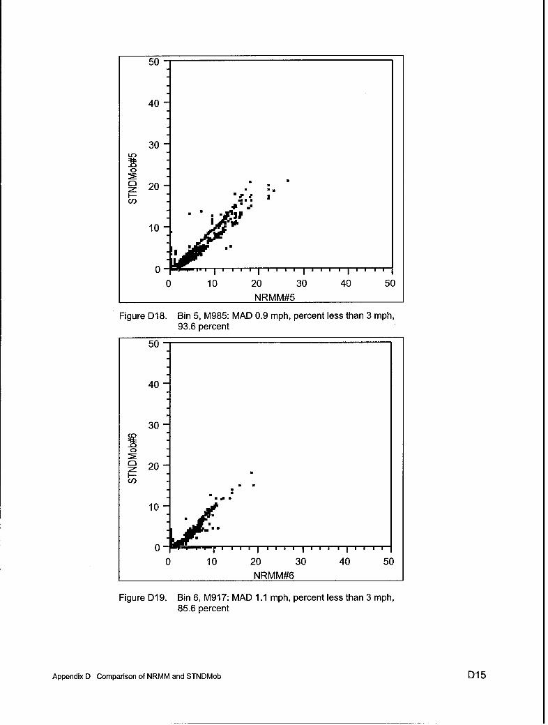
50

40

30

Ur)

10

20I.-II

3 .. . 3

0 10 20 30 40 50

NRMM#5


50

40

30

o' 20

10-

0 -

0 10 20 30 40 50NRMM#6



50

40

30

'20 20

I-.

U).

10

07- U o ~i I I 1 41 111 loo sli p I T II

0 10 20 30 40 50

NRMM#7


50

40

30

S20 •"

ci)

10 -"* I,

0-0 10 20 30 40 50

NRMM#8



50.0

40.0

30.0

0

S20.0I-.U)

10.0

0.0 f l l gl"

0 10 20 30 40 50

NRMM#9

Figure D22. Bin 9, M91 1-M747: MAD 0.63 mph, percent less than3 mph, 93.1 percent

50-

40

30

Q 20-1-

10

0 10 20 30 40 5ONRMM#10

Figure D23. Bin 10, M113A2: MAD 1.0 mph, percent less than 3 mph,94.4 percent


50

40

I :1 ,30

0 t

Q 20-I--

ci)

10

0 10 20 30 40 50

NRMM#11

Figure D24. Bin 11, LAV3: MAD 1.3 mph, percent less than 3 mph,85.1 percent

50

40

30

S20 ,

CO =

10 •

0I r 1-

0 10 20 30 40 50NRMM#12

Figure D25. Bin 12, Kawasaki ATV: MAD 1.6 mph, percent less than3 mph, 72.9 percent


This is a less than satisfactory match between the NRMM II andSTNDMob 3.2 predictions for Bin 12. Since the ATV is much smaller and has ahigh acceleration potential, NRMM is predicting substantially higher speedsbetween obstacles within 100 ft of one another. Therefore, for this vehicle, allterrain units whereby the obstacle spacing is greater than 50 ft were eliminated.This leaves 1265 terrain units. The changes to the comparison are shown inFigure D26.

50

40.Ei.

30

S20

100

CI)

0 . ... . *~ I .... . * . . . I . . . .I I . . . .I

0 10 20 30 40 50NRMM#12

Figure D26. Modified Bin 12, Kawasaki ATV: MAD 1.0 mph, percentless than 3 mph, 84.7 percent

Thus, with a fair comparison of how STNDMob 3.2 and NRMM 11.6.8model vehicle-obstacle interaction, 8 of the 12 representative vehicles predicted(67 percent) met the pass/fail criteria. Had the percent less than 3 mph beenrelaxed to 85 percent, then 11 of 12 representative vehicles predicted (92 percent)would have met the pass/fail criteria with the last just missing the mark.

Summary

From the results of this comparison, it can be stated with some degree ofstatistical confidence that for all 12 representative vehicles, STNDMob 3.2 andNRMM 11.6.8 are in agreement when the terrain considered does not go beyondthe capability for STNDMob 3.2 to model the interaction. When the terrain dataset was expanded to include what NRMM 11.6.8 can fully model, STNDMob 3.2was in agreement for 67 percent of the vehicles for the criteria stated.


Form ApprovedREPORT DOCUMENTATION PAGE OMB No. 0704-0188

Public reporting burden for this collection of information is estimated to average 1 hour per response, including the time for reviewing instructions, searching existing data sources, gathering and maintainingthe data needed, and completing and reviewing this collection of information. Send comments regarding this burden estimate or any other aspect of this collection of information, including suggestions forreducing this burden to Department of Defense, Washington Headquarters Services, Directorate for Information Operations and Reports (0704-0188), 1215 Jefferson Davis Highway, Suite 1204, Artington,VA 22202-4302. Respondents should be aware that notwithstanding any other provision of law, no person shall be subject to any penalty for failing to comply with a collection of information if it does not

display a currently valid OMB control number. PLEASE DO NOT RETURN YOUR FORM TO THE ABOVE ADDRESS.

1. REPORT DATE (DD-MM-YYYY) 2. REPORT TYPE 3. DATES COVERED (From - To)

February 2005 Final report

4. TITLE AND SUBTITLE 5a. CONTRACT NUMBER

Standard for Ground Vehicle Mobility 5b. GRANT NUMBER

5c. PROGRAM ELEMENT NUMBER62784/T40/154

6. AUTHOR(S) 5d. PROJECT NUMBER

E. Alex Baylot, Jr., Burhman Q. Gates, John G. Green, Paul W. Richmond, 5e. TASK NUMBER

Niki C. Goerger, George L. Mason, Chris L. Cummins, Laura S. Bunch

5f. WORK UNIT NUMBER

7. PERFORMING ORGANIZATION NAME(S) AND ADDRESS(ES) 8. PERFORMING ORGANIZATION REPORT

NUMBER

U.S. Army Engineer Research and Development Center, Geotechnical and StructuresLaboratory, 3909 Halls Ferry Road, Vicksburg, MS 39180-6199; ERDC/GSL TR-05-6North Wind, Inc., 3046 Indiana Avenue, Suite R, PMB 172, Vicksburg, MS 39180-5252

9. SPONSORING / MONITORING AGENCY NAME(S) AND ADDRESS(ES) 10. SPONSOR/MONITOR'S ACRONYM(S)

Office of Assistant Secretary of the Army for Acquisition, Logistics, and TechnologyWashington, DC 20310 11. SPONSOR/MONITOR'S REPORT

NUMBER(S)

12. DISTRIBUTION I AVAILABILITY STATEMENT

Approved for public release; distribution is unlimited.

13. SUPPLEMENTARY NOTES

14. ABSTRACTMobility implementation in military models and simulations (M&S) currently is tailored primarily for specific models, leading to

inconsistency between models. To assist decision-makers in analysis, acquisition, and training activities, it is necessary to provide andpromote consistency among the models.

The NATO Reference Mobility Model (NRMM), Version II, is the Army Battle Command, Simulation and ExperimentationDirectorate, standard for single vehicle ground movement representation. This report describes the development of an NRMM-basedStandard Mobility (STNDMob) Application Programming Interface (API) as a means of readily achieving higher fidelity movementrepresentation by incorporating terrain-limited speeds into M&S.

As described in the report, the STNDMob API, Version 3, includes descriptions of two derivative models: the low-resolution(Level 1) and the medium-resolution (Level 2) capabilities of STNDMob within the tactical/entity fidelity. Each level of resolution hastwo degrees of fidelity. These levels of resolution are an implementation of the physical models for steady-state speed conditions. As awhole, STNDMob can be classified as a service module that provides vehicle speeds to a vehicle routing service/planner.

(Continued)

15. SUBJECT TERMS Maneuver MovementCombat model Mobility model NRMMGround vehicle Modeling standards Vehicle traction

16. SECURITY CLASSIFICATION OF: 17. LIMITATION 18. NUMBER 19a. NAME OF RESPONSIBLEOF ABSTRACT OF PAGES PERSON

a. REPORT b. ABSTRACT c. THIS PAGE 19b. TELEPHONE NUMBER (include

UNCLASSIFIED UNCLASSIFIED UNCLASSIFIED 114 area code)

Standard Form 298 (Rev. 8-98)Prescribed by ANSI Std. 239.18

14. ABSTRACT (Concluded).

Included in the report are descriptions of the input/output data, algorithm process and supporting equations, andexample data. Appendixes provide supporting data descriptions, software documentation, and a comparison ofSTNDMob to NRMM.

standard for ground vehicle mobility - dtic

Documents