standard operating procedure saxs on the bruker …prism.mit.edu/xray/documents/edit in progress...

of 27

Revision Date: 8 March 2011

Standard Operating Procedure

SAXS

on the Bruker D8 Discover with GADDS

Scott A Speakman, Ph.D

Center for Materials Science and Engineering at MIT

For assistance in the X-ray Lab, contact Charles Settens

[email protected]

http://prism.mit.edu/xray

You must contact SEF staff at least 2 days in advance if you want to collect SAXS data on the

Bruker D8 with GADDS because the SAXS attachment needs to be put on the instrument. The

SAXS attachment takes 15 minutes to put on and requires 45 minutes before it can be used. The

SAXS attachment then requires 20 minutes to be removed. This time must be figured in to your

reservation.

The instrument allows features:

Incident-beam monochromator to remove K-beta and W L radiation from the X-ray spectrum

Choice of incident-beam collimators

When using this instrument, please remember the following warnings:

always check the shutter open/closed indicator inside the instrument enclosure

o the software does not always correctly indicate if the shutter is open or closed

do not touch the face of the detector

do not bump the video camera and laser- these are precisely aligned to give you good data

watch for collisions

o watch the sample stage to make sure that is does not hit the SAXS attachment

o watch the sample to make sure that it does not hit the collimator when OMEGA < 10deg

o do not drive OMEGA to an angle higher than 2THETA. If moving both positions, it is

usually better to drive one and then the other rather than driving both at the same time.

Use CTRL+C to stop an action- for example, if you need to prevent a collision when moving

a goniometer motor or collecting data.

If you are not near the keyboard and need to stop an action, hit the STOP button on the

instrument control column.

The tube operating power is 40 kV and 40 mA.

The tube standby power is 20 kV and 5 mA.

Do not turn the generator off- we want to always leave the instrument on.

mailto:[email protected]

of 27


1) Using GADDS to Collect Routine Data (a single set of scans)

A) Starting GADDS pg 2

B) Creating a New Project pg 3

C) Checking the Instrument Configuration pg 4-7

D) Mounting and Aligning the Sample pg 7-10

E) Turning the Generator Power Up pg 11

F) Collecting Data using a Single Run pg 11-13

2) Analyzing the Data

A) Loading Data pg 14

B) Using Cursors pg 14

C) Integrating Data to Produce a 1D plot for analysis pg 15

D) Merging Multiple Datasets pg 18

E) Plotting a Rocking Curve Graph pg 18

3) Using GADDS to Collect Multiple Datasets for Automated Mapping

A) MultiRuns for Pole Figure and other mapping pg 19

B) MultiTargets for XYZ mapping pg 21

Appendix A. Background on 2D Diffraction pg 23

Instructions for Planning a Texture Measurement using Multex Area are written in another SOP.

I. USING GADDS TO COLLECT ROUTINE DIFFRACTION DATA (A SINGLE SET OF SCANS)

1. Start GADDS

There are two versions of the GADDS software: GADDS and GADDS Off-Line.

GADDS communicates with the instrument and is used for data collection and analysis.

GADDS cannot be used to analyze data while it is also being used to collect data.

GADDS Off-Line does not communicate with the diffractometer and is used only for

data analysis.

Use GADDS Off-Line to analyze data when GADDS is being used to collect data.

1) Start the GADDS program.

a) A dialogue will ask if you want to set the generator power to 40 kV and 40 mA.

b) Click NO- do not turn up the generator power until after you have loaded your sample.

of 27


2. CREATE A NEW PROJECT OR OPEN AN EXISTING PROJECT

Projects are used to specify the folder where data will be saved and to set default values for the

title during data collection.

A. To create a new project

These instructions are designed for you to load a template project and then copy it. This will

load in the correct angle limits and other parameters for SAXS experiments.

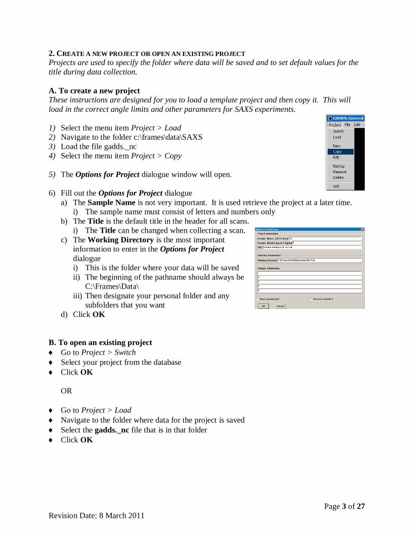
1) Select the menu item Project > Load

2) Navigate to the folder c:\frames\data\SAXS

3) Load the file gadds._nc

4) Select the menu item Project > Copy

5) The Options for Project dialogue window will open.

6) Fill out the Options for Project dialogue

a) The Sample Name is not very important. It is used retrieve the project at a later time.

i) The sample name must consist of letters and numbers only

b) The Title is the default title in the header for all scans.

i) The Title can be changed when collecting a scan.

c) The Working Directory is the most important

information to enter in the Options for Project

dialogue

i) This is the folder where your data will be saved

ii) The beginning of the pathname should always be

C:\Frames\Data\

iii) Then designate your personal folder and any

subfolders that you want

d) Click OK

B. To open an existing project

Go to Project > Switch

Select your project from the database

Click OK

OR

Go to Project > Load

Navigate to the folder where data for the project is saved

Select the gadds._nc file that is in that folder

Click OK

of 27


3. CHECK THE INSTRUMENT CONFIGURATION

A. Make sure that the generator power is at 20kV and 5mA

○ Go to Collect > Goniometer > Generator

○ Set the power to 20kV and 5mA

○ Click OK

B. Checking Instrument Status and Opening Doors

1) Before opening the enclosure doors

Look at the interior right-hand side of the enclosure. There is a black box

with several warning indicator lights.

The orange “X-RAY ON” lights should be lit. These indicate the generator

is on and the instrument is collecting data.

The green “SHUTTER CLOSED” lights should be lit.

If the green “SHUTTER CLOSED” lights are not lit or if the red

“SHUTTER OPEN” lights are lit, then do not open the doors.

o Look at the instrument computer and determine if a measurement is in

progress. If so, wait until it finishes or manually stop it by pressing

CTRL + C on the keyboard.

o If no measurement is in progress, then something is wrong. Do not

attempt to operate the instrument. Contact SEF staff to report the

problem

2) To open the enclosure doors

On either column on the lower sides of the instrument, find the green

“Open Door” button. Press this button to unlock the doors.

Pull the door handle out towards you. Gently slide the doors open.

To close the doors, gently slide the doors closed. Push the handles in

towards the instrument.

D. Check the Detector Distance The detector is usually positioned at 400mm for SAXS. To confirm the distance:

a) Read the position of the front edge of the detector mount using the scale on the

goniometer arm

b) Add 100mm to that number

c) This is the approximate detector distance.

The detector can be moved closer to the sample. This would allow data to be collected to larger

angles 2theta (WAXS) but would reduce the maximum d-spacing and the resolution of the data.

If you would like the detector to be closer to the sample, inform the SEF staff when you make

arrangements to have the SAXS attachment put on the instrument.

of 27


E. Check or Change the Detector Settings in the GADDS Software

Every time the Vantec-2000 detector is moved, the position of the detector must be recalibrated.

This means that the detector position might be slightly different each time you use the

instrument.

A note will be posted on the monitor of the data collection computer that will report the

current position of the detector. Confirm that these settings are configured in the software.

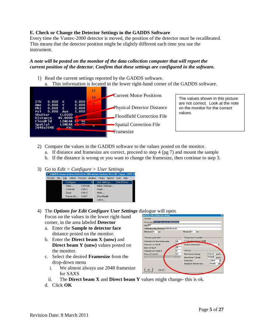
1) Read the current settings reported by the GADDS software.

a. This information is located in the lower right-hand corner of the GADDS software.

2) Compare the values in the GADDS software to the values posted on the monitor.

a. If distance and framesize are correct, proceed to step 4 (pg 7) and mount the sample

b. If the distance is wrong or you want to change the framesize, then continue to step 3.

3) Go to Edit > Configure > User Settings

4) The Options for Edit Configure User Settings dialogue will open.

Focus on the values in the lower right-hand

corner, in the area labeled Detector

a. Enter the Sample to detector face

distance posted on the monitor.

b. Enter the Direct beam X (unw) and

Direct beam Y (unw) values posted on

the monitor.

c. Select the desired Framesize from the

drop-down menu

i. We almost always use 2048 framesize

for SAXS

ii. The Direct beam X and Direct beam Y values might change- this is ok.

d. Click OK

The values shown in this picture are not correct. Look at the note on the monitor for the correct values.

Physical Detector Distance

Current Motor Positions

Floodfield Correction File

Spatial Correction File

Framesize

of 27


5) A pop-up message may ask if you want to reset the goniometer limits

a. Click NO

b. It is very important that you do not reset the goniometer limits—doing so may prevent

you from collecting the data that you want.

6) A pop-up message will ask if you want to load the new spatial

and floodfield correction files. Click Yes.

a. If an error message tells you that the Flood Correction

could not be loaded or that the Flood correction

files were collected at a different distance, do not

worry. This is alright—just click OK.

Note: you can change the Framesize that you want to use.

The framesize dictates how many pixels the detector will be divided into, and therefore affects

the resolution of the data. A higher resolution can produce better peak shapes and angular

resolution but will also produce larger files.

A 2048x2048 resolution produces 4 MB files.

o We almost always use this for SAXS.

A 1024x1024 resolution produces 1 MB files.

o This is the preferred resolution if you are analyzing pole figures of textured materials.

A 512x512 resolution produces 0.5 MB files

o Do not use this framesize

Not all framesizes are available for all detector positions. The allowed combinations are:

Detector Distance Framesize Floodfield name Spatial name

160 mm 2048 2048_016 2048_016

160 mm 1024 1024_016 1024_016

290 mm 2048 2048_029 2048_029

300 mm 2048 2048_030 2048_030

300 mm or larger any linear linear

Sometimes the correct floodfield or spatial file does not load. If this happens, manually load the

correct floodfield and spatial files

Go to Process > Flood > Load

o Click on the … button to open the folder of correction files

o Select the appropriate *._fl file in the folder C:\frames\Calib\

Go to Process > Spatial > Load

o Click on the … button to open the folder of correction files

o Select the appropriate *._ix file in the folder C:\frames\Calib\

of 27


4. MOUNT AND ALIGN THE SAMPLE

A. First, check that the generator power is at 20kV and 5mA

○ If it is not, go to Collect > Goniometer > Generator

○ Set the power to 20kV and 5mA

○ Click OK

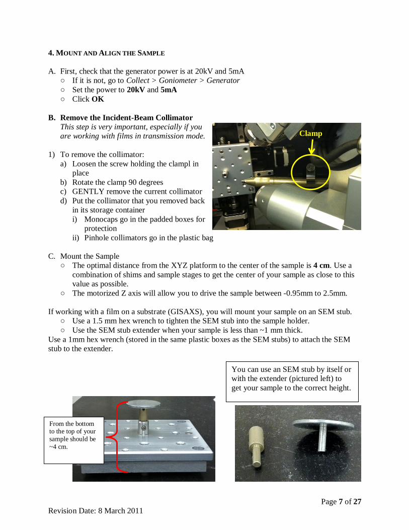
B. Remove the Incident-Beam Collimator

This step is very important, especially if you

are working with films in transmission mode.

1) To remove the collimator:

a) Loosen the screw holding the clampl in

place

b) Rotate the clamp 90 degrees

c) GENTLY remove the current collimator

d) Put the collimator that you removed back

in its storage container

i) Monocaps go in the padded boxes for

protection

ii) Pinhole collimators go in the plastic bag

C. Mount the Sample

○ The optimal distance from the XYZ platform to the center of the sample is 4 cm. Use a

combination of shims and sample stages to get the center of your sample as close to this

value as possible.

○ The motorized Z axis will allow you to drive the sample between -0.95mm to 2.5mm.

If working with a film on a substrate (GISAXS), you will mount your sample on an SEM stub.

○ Use a 1.5 mm hex wrench to tighten the SEM stub into the sample holder.

○ Use the SEM stub extender when your sample is less than ~1 mm thick.

Use a 1mm hex wrench (stored in the same plastic boxes as the SEM stubs) to attach the SEM

stub to the extender.

Clamp

From the bottom to the top of your

sample should be

~4 cm.

You can use an SEM stub by itself or

with the extender (pictured left) to

get your sample to the correct height.

of 27


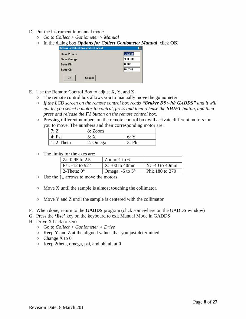
D. Put the instrument in manual mode

○ Go to Collect > Goniometer > Manual

○ In the dialog box Options for Collect Goniometer Manual, click OK

E. Use the Remote Control Box to adjust X, Y, and Z

○ The remote control box allows you to manually move the goniometer

○ If the LCD screen on the remote control box reads “Bruker D8 with GADDS” and it will

not let you select a motor to control, press and then release the SHIFT button, and then

press and release the F1 button on the remote control box.

○ Pressing different numbers on the remote control box will activate different motors for

you to move. The numbers and their corresponding motor are:

7: Z 8: Zoom

4: Psi 5: X 6: Y

1: 2-Theta 2: Omega 3: Phi

○ The limits for the axes are:

Z: -0.95 to 2.5 Zoom: 1 to 6

Psi: -12 to 92° X: -00 to 40mm Y: -40 to 40mm

2-Theta: 0° Omega: -5 to 5° Phi: 180 to 270

○ Use the ↑↓ arrows to move the motors

○ Move X until the sample is almost touching the collimator.

○ Move Y and Z until the sample is centered with the collimator

F. When done, return to the GADDS program (click somewhere on the GADDS window)

G. Press the ‘Esc’ key on the keyboard to exit Manual Mode in GADDS

H. Drive X back to zero

○ Go to Collect > Goniometer > Drive

○ Keep Y and Z at the aligned values that you just determined

○ Change X to 0

○ Keep 2theta, omega, psi, and phi all at 0

of 27


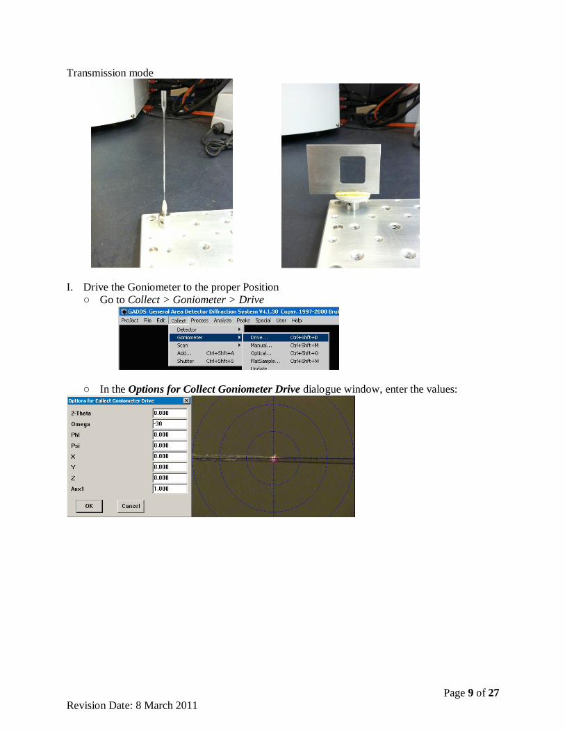
Transmission mode

I. Drive the Goniometer to the proper Position

○ Go to Collect > Goniometer > Drive

○ In the Options for Collect Goniometer Drive dialogue window, enter the values:

of 27


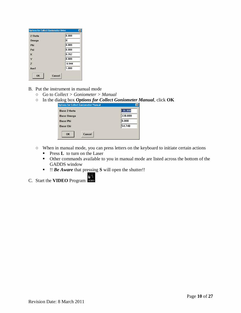
B. Put the instrument in manual mode

○ Go to Collect > Goniometer > Manual

○ In the dialog box Options for Collect Goniometer Manual, click OK

○ When in manual mode, you can press letters on the keyboard to initiate certain actions

Press L to turn on the Laser

Other commands available to you in manual mode are listed across the bottom of the

GADDS window

!! Be Aware that pressing S will open the shutter!!

C. Start the VIDEO Program

of 27


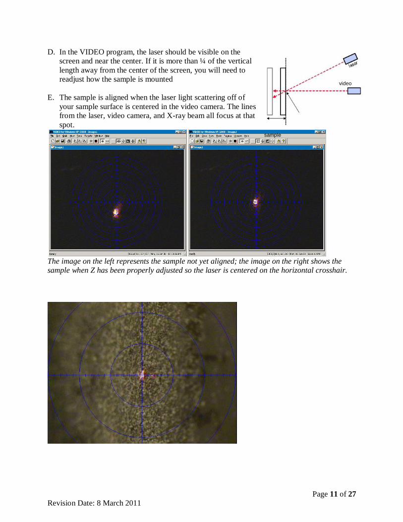
D. In the VIDEO program, the laser should be visible on the

screen and near the center. If it is more than ¼ of the vertical

length away from the center of the screen, you will need to

readjust how the sample is mounted

E. The sample is aligned when the laser light scattering off of

your sample surface is centered in the video camera. The lines

from the laser, video camera, and X-ray beam all focus at that

spot.

The image on the left represents the sample not yet aligned; the image on the right shows the

sample when Z has been properly adjusted so the laser is centered on the horizontal crosshair.

video

sample

of 27


Check and Change the Incident-Beam Collimator

There are two different styles of collimator in a variety of sizes that you can use.

Monocapillary (fiber-optic) collimators produce a high-intensity but more divergent beam

○ Use the 0.3mm or 0.05mm diameter for SAXS

Pinhole collimators produce tighter collimation and better resolution,

○ Use the 0.5mm, 0.1mm, or 0.05mm diameters sizes for SAXS

Collimation, detector distance, and the size of the beam stop determine the resolution of the

SAXS system. The maximum resolvable size is the either R (the resolution limit of the

collimator) or Rbs (the resolution limit of the beam stop) whichever is smaller. The values

below are for when the detector is at 300 mm distance.

Pinhole Collimator α1 (°) D (mm) αmax(°) R (Å) Rbs (Å)

0.05 0.04 0.071 0.09 951 231

0.10 0.08 0.143 0.15 599 231

0.30 0.23 0.418 0.34 257 231

0.50 0.27 0.639 0.43 207 231

2) Read the label on the collimator to determine what type and size is currently mounted.

The monocapillary collimator has the size stamped into the metal.

The pinhole collimator has the size labeled with white text on black background.

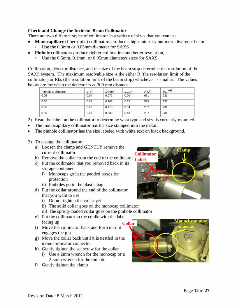
3) To change the collimator:

a) Loosen the clamp and GENTLY remove the

current collimator

b) Remove the collar from the end of the collimator

c) Put the collimator that you removed back in its

storage container

i) Monocaps go in the padded boxes for

protection

ii) Pinholes go in the plastic bag

d) Put the collar around the end of the collimator

that you want to use

i) Do not tighten the collar yet

ii) The solid collar goes on the monocap collimator

iii) The spring-loaded collar goes on the pinhole collimator

e) Put the collimator in the cradle with the label

facing up

f) Move the collimator back and forth until it

engages the pin

g) Move the collar back until it is nestled in the

monochromator connector

h) Gently tighten the set screw for the collar

i) Use a 2mm wrench for the monocap or a

2.5mm wrench for the pinhole

i) Gently tighten the clamp

Collimator

Label

Clamp

Collar Monochromator

Connector

of 27


5. TURN THE GENERATOR POWER UP

Go to Collect > Goniometer > Generator

Set the tube power to 40 kV and 40 mA

Click OK

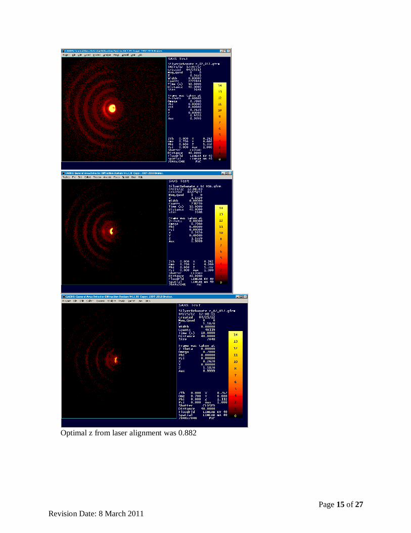
If working with GI-SAXS (film on substrate), then you need to finish the alignment with

some omega and z scans

of 27


of 27


Optimal z from laser alignment was 0.882

of 27


Use f10 button

Collect a long scan to use for calibration of the sample-detector distance

Select the menu Process> calibrate

of 27


J.

K.

L.

of 27


M. N.

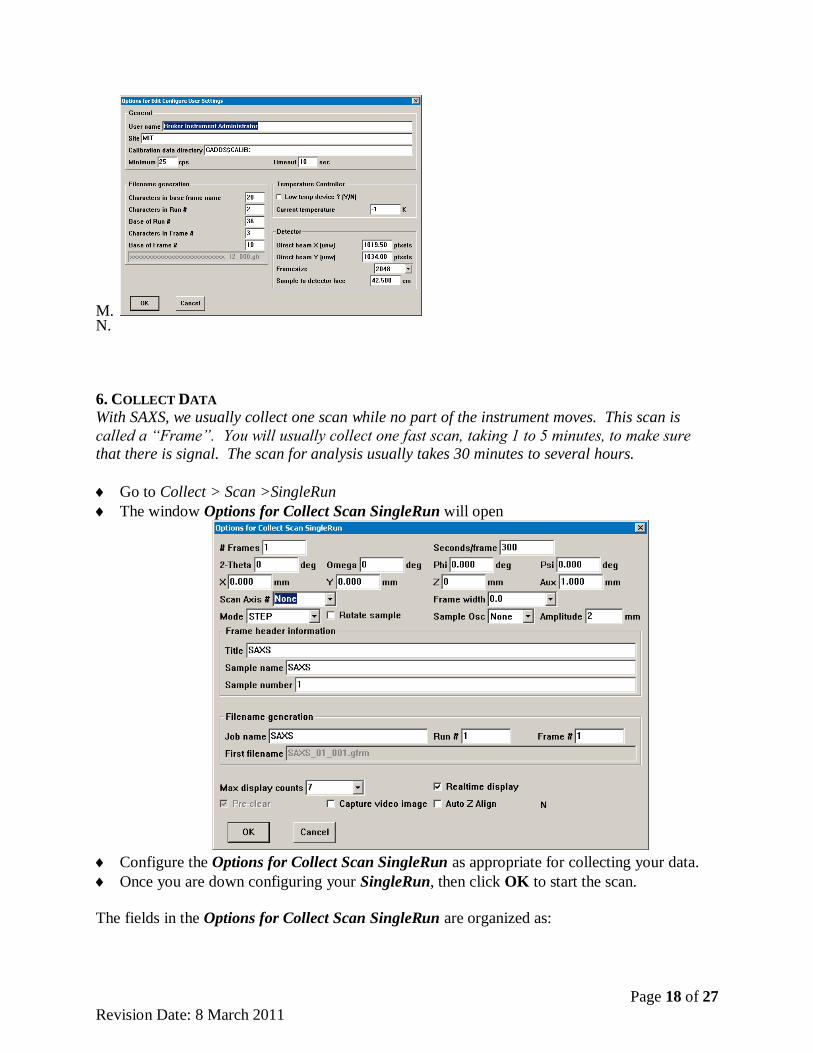
6. COLLECT DATA

With SAXS, we usually collect one scan while no part of the instrument moves. This scan is

called a “Frame”. You will usually collect one fast scan, taking 1 to 5 minutes, to make sure

that there is signal. The scan for analysis usually takes 30 minutes to several hours.

Go to Collect > Scan >SingleRun

The window Options for Collect Scan SingleRun will open

Configure the Options for Collect Scan SingleRun as appropriate for collecting your data.

Once you are down configuring your SingleRun, then click OK to start the scan.

The fields in the Options for Collect Scan SingleRun are organized as:

of 27


Data Collection Options (the upper portion of the dialog window)

○ # Frames- how many frames of diffraction data will be collected.

Almost always 1

○ Seconds/Frame- how long the detector will be exposed for each frame

you can enter this information as hh:mm:ss or as an integer value for seconds.

60 to 300 seconds/frame is a typical time for fast scans

Slow data collection may take as long as 1800 or 3600 seconds/frame (0.5 or 1 hr)

○ 2-Theta, Omega, Phi, Psi, X, Y, Z- starting positions for these axes during the first frame

Make sure that X, Y, and Z properly reflect the aligned position for the sample that you

determined in step 4 (pg 6-8). These positions do not always update in the SingleRun to

reflect your alignment

You can read the current positions of all axes in the lower right-hand corner of the

GADDS program window.

The limits for the axes are:

2-Theta: -6 to 102° X: -40 to

40mm

Omega: -30 to

100°

Y: -40 to

40mm

Psi: -12 to 92° Z: -0.95 to 2.5

Aux is the video camera zoom. This number should be between 1 to 6.

○ Scan Axis #- this is the position/motor that will change between subsequent frames.

Select an option from the drop-down menu

Unless aligning a sample for GISAXS, this will be None

Options are: 1 2T, 2 Om, 3 Phi, 4 Psi, 5 X, 6 Y, 7 Z, 8 Aux, None, and Coupled

Never select 1 2T, 5 X, or Coupled—moving these motors may cause a collision

Om is the Omega angle

○ Frame width- how much the Scan Axis will change between each frame.

○ Mode- how the Scan Axis will change during the run. The options are:

Step (the most common choice): the first frame is collected, then the scan axis changes by

the frame width and the next frame is collected

Scan: as the frame is being collected, the scan axis changes by the frame width. The

frame represents the sum of the signal observed while the scan axis was moving.

Oscillate: the scan axis will oscillate by the frame width during the data collection

○ Rotate Sample Never check this option!!!!

○ Sample Osc This should always be NONE!!!!

Frame Header Information These are miscellaneous information that will be recorded in the data for record-keeping

purposes. You can use these fields in any manner that makes sense to you

Title is inherited from the Title in the project (step 1), but it can be changed

○ some people use title to indicate the overall research project, other people use it to

indicate details specific to that data scan

Sample name is not inherited from the sample name that you entered when creating a

project, but rather will be the value last entered in GADDS

○ some people use the sample name to record details of the sample or of the instrument

of 27


configuration, such as the beam size

Filename generation These settings are used to generate the filename(s) for each frame from the SingleRun

Job Name-- this makes up the prefix of the filename

○ Limited to 26 characters

Run #-- this will be held constant during a SingleRun

○ Usually this is used to differentiate slightly different measurements from the same

sample, for example if you collected on SingleRun with the sample stationary and

another SingleRun with the sample rotating or oscillating

Frame #-- this will change between different frames in the SingleRun measurement

Other options

Max Display-- the y axis (intensity) maximum value during realtime display of data

○ The intensity does not autoscale during data collection, so you have to guess what the

maximum intensity should be.

○ Typical choices are 7, 15, or 31

Realtime display- check this option to show the diffraction data during the measurement

Capture video image- check this option to save the image from the video camera before

each frame

Auto Z align- never check this option

The example shown on the previous page will collect 5 frames of data. The first frame will be

collected with the detector centered at 2-Theta=30deg and Omega=15deg. In between each

subsequent scan, 2-Theta will change by 15deg and Omega will change by 7.5deg. Each of the 5

frames will be collected for 60 seconds, and the sample will rotate about Phi while the frame is

being collected.

○ This type of measurement will produce diffraction data from 17 to 103deg 2-Theta.

of 27


II. ANALYZING THE DATA The last frame collected will be shown in GADDS when the measurement is finished.

1. To navigate through frames after data collection is finished:

Ctrl + Right Arrow keys will go to the next frame # for a given run #

Ctrl + Left Arrow keys will go to the previous frame # for a given run #

2. To load other data frames

Go to File > Display > Open

o You can also use File > Load to open a frame

o You will have access to different options depending which one you use

The File > Display > Open dialog The File > Load dialog

3. Using Cursors for Determining Peak Positions and Intensities

In the GADDS program, you can activate various cursors that will allow you to extract

approximate values for peak positions and intensities.

Go to Analyze > Cursors

Select a cursor

On-screen instructions in the bottom of the GADDS

window show you options for manipulating that

cursor

○ Conic cursor (shown to the right): you control a

point (indicated by cross-hairs). The information

area shows you the intensity and position of the

point.

You are also shown an arc. All data along that arc corresponds to the same 2-Theta

value (it is the arc of the Debye Diffraction Ring)

You can use this arc to determine the position of a peak and if different spots belong

to the same 2-Theta peak position

○ Rbox cursor: you control a box. You are given statistics for the intensity inside the box

(total counts, maxium counts, mean counts)

To change the size of the box, right-click and then drag the mouse. Right-click again

when the box is the size that you want.

!! In GADDS, the 2Theta axis goes from right to left. The center of the data shown is the

2Theta that you specified; the rightside portion of the data are the lower 2Theta values; and

the leftside portion of the data are the higher 2Theta values !!

of 27


4. To Convert Data into a 1D Scan In order to analyze 2D data, we usually need to convert the data into a 1D scan (intensity vs 2-Theta). We do this by

integrating the data along Debye Rings into a single data point. Data can be converted using Chi Integration or

Slices. Data can also be converted using a separate program called Pilot—this program is especially useful if you

have multiple frames that you want to combine together. Once 2D data are converted into a 1D plot, you can load

the data into HighScore Plus for analysis.

A. To use Chi Integration

With Chi integration, the integration area is constrained so that an equal

arc length is used for each 2Theta position

Open the frame that you want to analyze

Go to Peaks > Integrate > Chi

In the window Options for Peaks Integrate Chi, you will set several

parameters. The most important parameters are Normalize Intensity

and Step Size

○ If you have established values for 2theta and Chi ranges that you want to use, input them here Otherwise, we will graphically edit the 2theta and Chi ranges in the next step, so don’t worry about

changing these values

○ The typical options for Normalize Intensity are: 3- Normalize by solid angle (quick approximation, peaks are broader and noisier)

Conic lines spaced by the specified step size are defined. The intensity for each pixel that

intersects the conic line is summed, and then normalized by the length of the arc in the gamma

direction.

5- Bin normalized (preferred, slower but more accurate)

Integration bins covering the specified step size are defined. The intensity for each pixel inside

that arc, using fractional area as a weighting factor, is summed and then normalized by the

fractional area of all of the pixels inside the bin.

○ The best Step size depends on the framesize and detector

distance. For detector distance >20cm or framesize 2048, use

.02

For detector distance <20cm and framesize 1024,

use .04

○ Click OK

The total area of the frame that will be analyzed is outlined in

the GADDS windows

You can adjust the integration arc by pressing 1, 2, 3, or 4 on

your keyboard and moving the mouse

○ Remember that 2theta goes from right to left for low to high value

○ 1 selects the starting 2theta (right edge)

○ 2 selects the ending 2theta (left edge)

○ 3 selects the starting chi (upper edge)

○ 4 selects the ending chi (lower edge)

○ Left-click once to stop changing the edges

Once the proper range is selected, left-click to integrate

The Integrate Options dialog opens

○ Enter any value for Title and File name

○ Format should be DIFFRACplus for the Bruker binary format Plotso is the Bruker Ascii format

○ If you check Append Y/N, then every frame that you integrate that has the same filename will actually be written into the same file. If unchecked, each frame must have a

different filename and will be written into a different file.

Click OK to save the integrated 1D scan

of 27


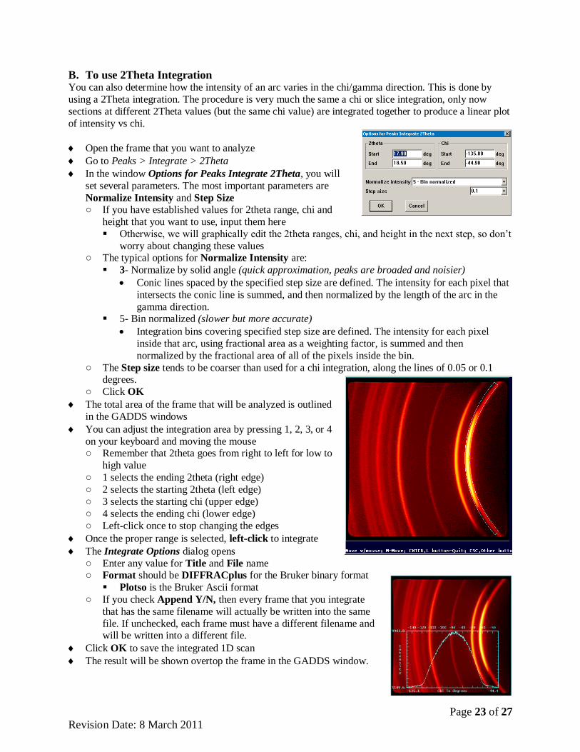
B. To use 2Theta Integration You can also determine how the intensity of an arc varies in the chi/gamma direction. This is done by

using a 2Theta integration. The procedure is very much the same a chi or slice integration, only now

sections at different 2Theta values (but the same chi value) are integrated together to produce a linear plot

of intensity vs chi.

Open the frame that you want to analyze

Go to Peaks > Integrate > 2Theta

In the window Options for Peaks Integrate 2Theta, you will

set several parameters. The most important parameters are

Normalize Intensity and Step Size ○ If you have established values for 2theta range, chi and

height that you want to use, input them here

Otherwise, we will graphically edit the 2theta ranges, chi, and height in the next step, so don’t

worry about changing these values ○ The typical options for Normalize Intensity are:

3- Normalize by solid angle (quick approximation, peaks are broaded and noisier)

Conic lines spaced by the specified step size are defined. The intensity for each pixel that

intersects the conic line is summed, and then normalized by the length of the arc in the

gamma direction. 5- Bin normalized (slower but more accurate)

Integration bins covering specified step size are defined. The intensity for each pixel

inside that arc, using fractional area as a weighting factor, is summed and then

normalized by the fractional area of all of the pixels inside the bin.

○ The Step size tends to be coarser than used for a chi integration, along the lines of 0.05 or 0.1 degrees.

○ Click OK

The total area of the frame that will be analyzed is outlined

in the GADDS windows

You can adjust the integration area by pressing 1, 2, 3, or 4

on your keyboard and moving the mouse ○ Remember that 2theta goes from right to left for low to

high value

○ 1 selects the ending 2theta (right edge)

○ 2 selects the starting 2theta (left edge)

○ 3 selects the starting chi (upper edge)

○ 4 selects the ending chi (lower edge)

○ Left-click once to stop changing the edges

Once the proper range is selected, left-click to integrate

The Integrate Options dialog opens

○ Enter any value for Title and File name ○ Format should be DIFFRACplus for the Bruker binary format

Plotso is the Bruker Ascii format

○ If you check Append Y/N, then every frame that you integrate

that has the same filename will actually be written into the same

file. If unchecked, each frame must have a different filename and will be written into a different file.

Click OK to save the integrated 1D scan

The result will be shown overtop the frame in the GADDS window.

of 27


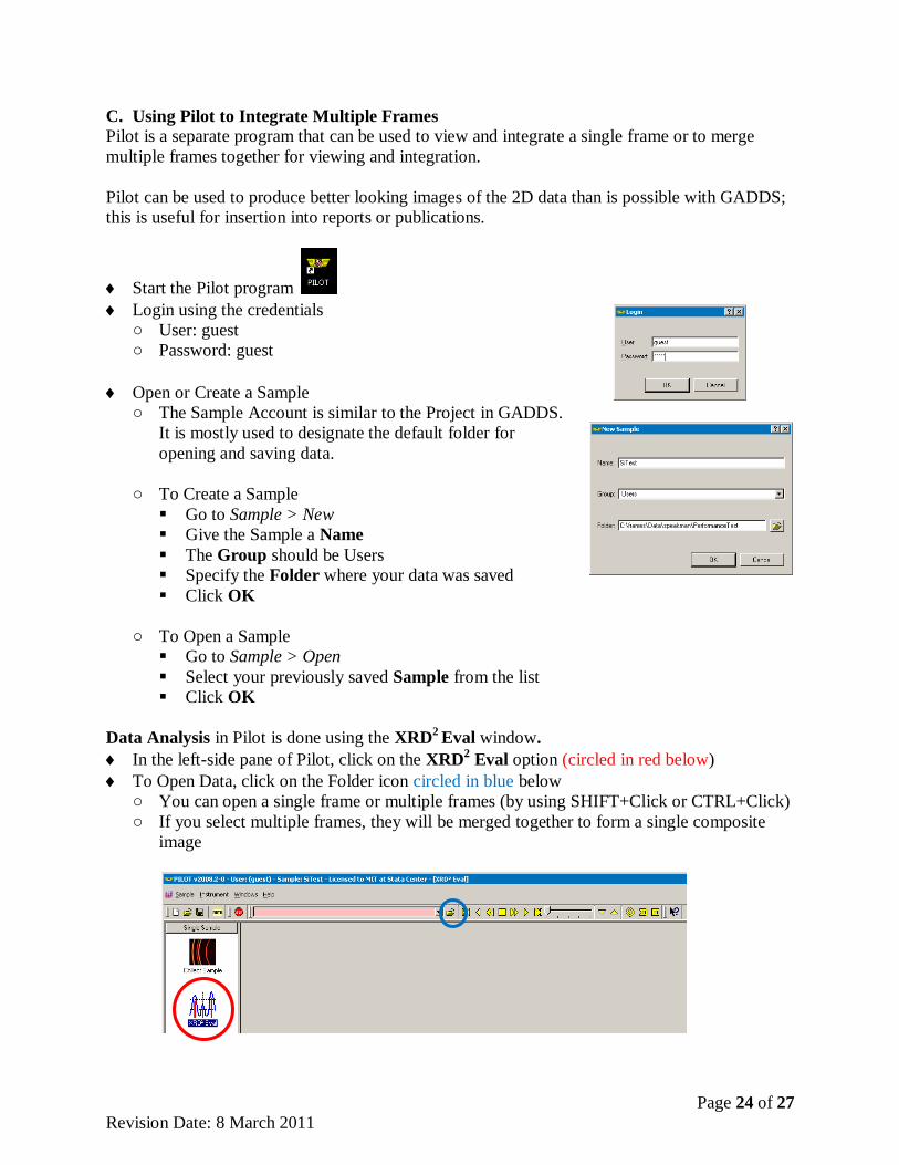
C. Using Pilot to Integrate Multiple Frames Pilot is a separate program that can be used to view and integrate a single frame or to merge

multiple frames together for viewing and integration.

Pilot can be used to produce better looking images of the 2D data than is possible with GADDS;

this is useful for insertion into reports or publications.

Start the Pilot program

Login using the credentials

○ User: guest

○ Password: guest

Open or Create a Sample

○ The Sample Account is similar to the Project in GADDS.

It is mostly used to designate the default folder for

opening and saving data.

○ To Create a Sample

Go to Sample > New

Give the Sample a Name

The Group should be Users

Specify the Folder where your data was saved

Click OK

○ To Open a Sample

Go to Sample > Open

Select your previously saved Sample from the list

Click OK

Data Analysis in Pilot is done using the XRD2 Eval window.

In the left-side pane of Pilot, click on the XRD2 Eval option (circled in red below)

To Open Data, click on the Folder icon circled in blue below

○ You can open a single frame or multiple frames (by using SHIFT+Click or CTRL+Click)

○ If you select multiple frames, they will be merged together to form a single composite

image

of 27


Manipulating the Color and Intensity Scale

Once you have data opened, you can easily change the brightness, contrast, and color

Underneath the image of the data are sliders to adjust the minimum and maximum intensity

○ The left-most slider sets the minimum intensity (circled in red)

any pixel with that many counts or fewer will be plotted as black

○ The right-most slider sets the maximum intensity (circled in blue)

any pixel with that many counts or more will be plotted as white

○ Moving both sliders left/right adjusts the brightness of the image

○ Changing the distance between the sliders adjusts the contrast of the image

Right-click in the color scale on the right of the Pilot program to change the color scheme.

○ The default color scheme is BB, which is based on black-body radiation

○ The PRINT color scheme is a grayscale that is useful for reports and publications

○ Change the Intensity to a LOG plot if you have both strong and weak features in the data

Changing the 2Theta Direction

As plotted by default, the frame shows data with 2Theta increasing from right to left

You can reverse the frame image, so that the data are plotted with the more traditional

manner of 2Theta increasing from left to right:

○ Right-click inside the frame area

○ Select Flip Image

To Save the Image the 2D Data

Right-click inside the frame area

Select Save PNG

Specify the filename and folder in the next window and click OK

of 27


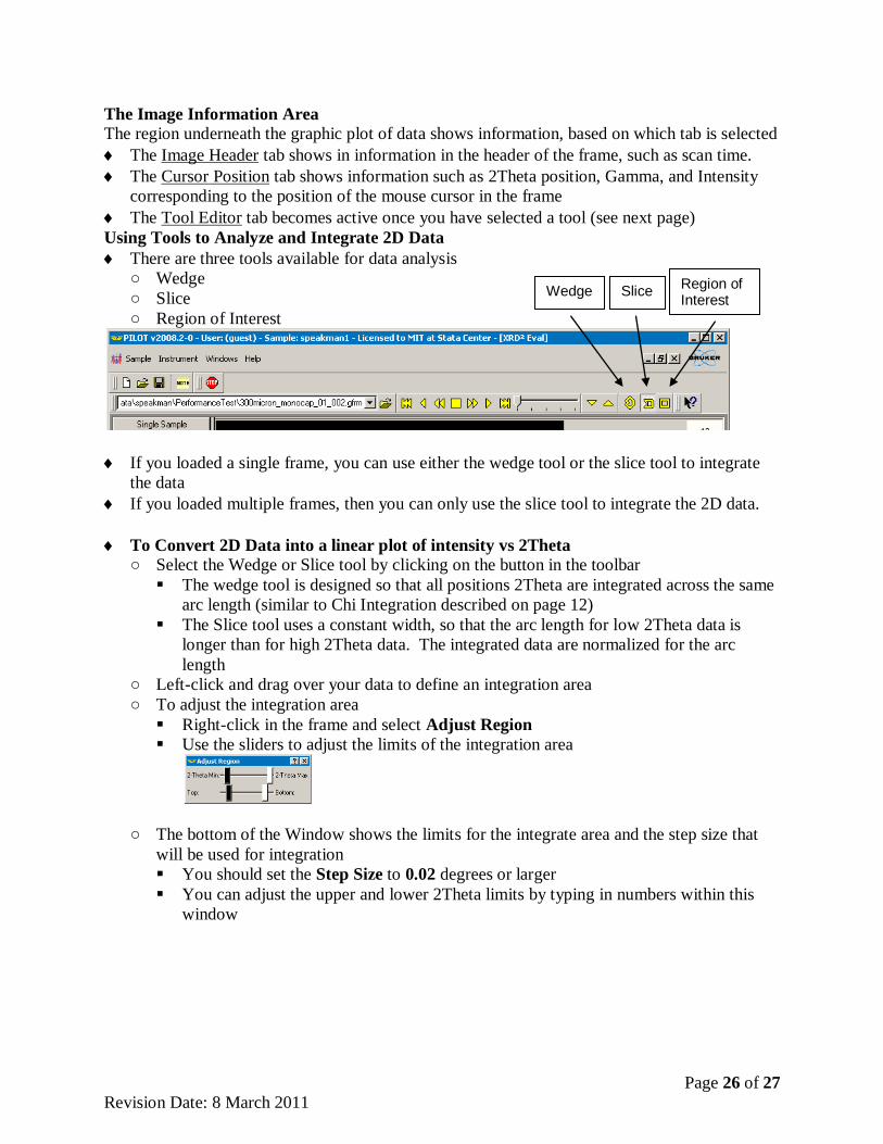
The Image Information Area

The region underneath the graphic plot of data shows information, based on which tab is selected

The Image Header tab shows in information in the header of the frame, such as scan time.

The Cursor Position tab shows information such as 2Theta position, Gamma, and Intensity

corresponding to the position of the mouse cursor in the frame

The Tool Editor tab becomes active once you have selected a tool (see next page)

Using Tools to Analyze and Integrate 2D Data

There are three tools available for data analysis

○ Wedge

○ Slice

○ Region of Interest

If you loaded a single frame, you can use either the wedge tool or the slice tool to integrate

the data

If you loaded multiple frames, then you can only use the slice tool to integrate the 2D data.

To Convert 2D Data into a linear plot of intensity vs 2Theta

○ Select the Wedge or Slice tool by clicking on the button in the toolbar

The wedge tool is designed so that all positions 2Theta are integrated across the same

arc length (similar to Chi Integration described on page 12)

The Slice tool uses a constant width, so that the arc length for low 2Theta data is

longer than for high 2Theta data. The integrated data are normalized for the arc

length

○ Left-click and drag over your data to define an integration area

○ To adjust the integration area

Right-click in the frame and select Adjust Region

Use the sliders to adjust the limits of the integration area

○ The bottom of the Window shows the limits for the integrate area and the step size that

will be used for integration

You should set the Step Size to 0.02 degrees or larger

You can adjust the upper and lower 2Theta limits by typing in numbers within this

window

Wedge Slice Region of Interest

of 27


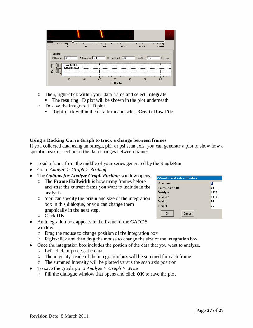
○ Then, right-click within your data frame and select Integrate

The resulting 1D plot will be shown in the plot underneath

○ To save the integrated 1D plot

Right-click within the data from and select Create Raw File

Using a Rocking Curve Graph to track a change between frames

If you collected data using an omega, phi, or psi scan axis, you can generate a plot to show how a

specific peak or section of the data changes between frames.

Load a frame from the middle of your series generated by the SingleRun

Go to Analyze > Graph > Rocking

The Options for Analyze Graph Rocking window opens.

○ The Frame Halfwidth is how many frames before

and after the current frame you want to include in the

analysis

○ You can specify the origin and size of the integration

box in this dialogue, or you can change them

graphically in the next step.

○ Click OK

An integration box appears in the frame of the GADDS

window

○ Drag the mouse to change position of the integration box

○ Right-click and then drag the mouse to change the size of the integration box

Once the integration box includes the portion of the data that you want to analyze,

○ Left-click to process the data

○ The intensity inside of the integration box will be summed for each frame

○ The summed intensity will be plotted versus the scan axis position

To save the graph, go to Analyze > Graph > Write

○ Fill the dialogue window that opens and click OK to save the plot

standard operating procedure saxs on the bruker …prism.mit.edu/xray/documents/edit in progress...

Documents