standard operating procedures for field samplers · pdf filestandard operating procedures for...
TRANSCRIPT
STANDARD OPERATING PROCEDURES FOR FIELD SAMPLERS
VOLUME II
BIOLOGICAL AND HABITAT SAMPLING
STATE OF SOUTH DAKOTA DEPARTMENT OF ENVIRONMENT AND NATURAL RESOURCES
WATER RESOURCES ASSISTANCE PROGRAM
STEVEN M. PIRNER, SECRETARY
FEBRUARY, 2005

STANDARD OPERATING PROCEDURES FOR FIELD SAMPLERS
VOLUME II
BIOLOGICAL AND HABITAT SAMPLING
Prepared by
Water Resources Monitoring Team
STATE OF SOUTH DAKOTA DEPARTMENT OF ENVIRONMENT AND NATURAL RESOURCES
WATER RESOURCES ASSISTANCE PROGRAM
STEVEN M. PIRNER, SECRETARY
Revision 1.2
February, 2005

TABLE OF CONTENTS
1.0 PRE-SAMPLING PROCEDURES .....................................................................................1
2.0 MACROPHYTE SURVEY .................................................................................................1 A. Purpose.....................................................................................................................1 B. Materials ..................................................................................................................1 C. Procedures................................................................................................................2
3.0 PHYTOPLANKTON SAMPLING .....................................................................................1 A. Purpose.....................................................................................................................1 B. Materials ..................................................................................................................1 C. In-lake Sampling......................................................................................................1 D. Tributary Sampling ..................................................................................................4 E. Shipping the Sample ................................................................................................5 F. SD DENR Algal Analysis Procedures.....................................................................5
4.0 ZOOPLANKTON SAMPLING ..........................................................................................1 A. Purpose.....................................................................................................................1 B. Materials ..................................................................................................................1 C. Zooplankton Sampling.............................................................................................1 D. Shipping the Sample ................................................................................................4 E. SD DENR Zooplankton Analysis Procedure...........................................................4
5.0 TRIBUTARY PERIPHYTON SAMPLING .......................................................................1 A. Purpose.....................................................................................................................1 B. Procedures................................................................................................................1
1. Natural Substrates ........................................................................................1 Erosional habitats:........................................................................................2 Depositional habitats: ..................................................................................3
2. Artificial Substrates .....................................................................................3 C. Sample Preparation and Preservation ......................................................................4

TABLE OF CONTENTS (continued
6.0 BENTHIC MACROINVERTEBRATE SAMPLING FOR WADEABLE STREAMS ...........................................................................................................................1 A. Purpose.....................................................................................................................1 B. Procedures................................................................................................................1
1. Identifying the Sampling Reach ..................................................................1 2. Sampling Procedure: Natural Substrates .....................................................3
a. Riffle/Run Habitat............................................................................3 b. Pool/Glide Habitat: ..........................................................................4 c. Narrow Channel:..............................................................................5 d. Deep Channel:..................................................................................6
C. Field Sampling QA/QC..........................................................................................10 D. Laboratory Procedures for Macroinvertebrate Identification ................................11 E. Laboratory QA/QC ................................................................................................13
7.0 ALTERNATE METHODS FOR TRIBUTARY AND IN-LAKE BENTHIC MACROINVERTEBRATE SAMPLING.........................................................1 A. Purpose .....................................................................................................................1 B. Materials ..................................................................................................................1 C. Site Selection ...........................................................................................................1
Tributary ..................................................................................................................1 In-lake ......................................................................................................................3
D. Water Chemistry ......................................................................................................3 E. Sampler Selection ....................................................................................................4 F. Benthic Macroinvertebrate Sampling Procedures ...................................................6 G. Quality Assurance/Quality Control Procedures (QA/QC).......................................9
8.0 PROCEDURE TO ESTABLISH AND USE PHOTO POINTS .........................................1 A. Photo Point Location ...............................................................................................1 B. Equipment ................................................................................................................1 C. Photo Point Procedure .............................................................................................2 D. Photo Point Data Management ................................................................................2 E. Photo Point Interpretation........................................................................................3
9.0 PHYSICAL HABITAT CHARACTERIZATION ..............................................................1 A. Introduction..............................................................................................................1
10.0. REFERENCE CITED............................................................................................................1

LIST OF FIGURES Figure 2.0.1. Aquatic Plant Survey Diagram. ................................................................... 3

LIST OF TABLES Table 2.0.1 SD WRAP Lake Habitat Assessment Field Data Sheet—Macrophyte Survey
..................................................................................................................................... 6 Table 9.0.1. Channel unit and Pool Forming element categories. ................................... 12

APPENDICES
Appendix A Lake Habitat Assessment Field Data Sheet — Macrophyte Survey Appendix B South Dakota WRAP In-lake Sampling Field Data Collection Sheet Appendix C South Dakota Water Quality Data Sheet Appendix D Periphyton Sampling Data Sheet Appendix E Macroinvertebrate Sampler Construction and Sampling Data Sheet Appendix F Habitat Field Collection Data Sheets
Section 1.0 Page 1 of 1 Revision 1.2
1.0 PRE-SAMPLING PROCEDURES
Each field investigation must be evaluated and designed on an individual basis. Common procedures addressed in developing an assessment workplan include the following:
1. Determine the objectives for sampling. 2. Review existing information and data on the waterbody under investigation. 3. Obtain adequate maps and diagrams to define the study area. 4. Conduct field reconnaissance of the proposed study area. 5. Develop a list of proposed sampling sites, sampling frequency, and sample
analysis. 6. Arrange schedules, responsibilities, funding and contracts with all agencies,
sponsors and laboratories involved with the study. 7. If sampling near or on private land, secure permission prior to deployment. 8. Coordinate all activities. 9. Develop a list of necessary equipment and supplies. 10. Check the operation of all equipment prior to field use.

Section 2.0 Page 1 of 6 Revision 1.2
2.0 MACROPHYTE SURVEY
A. Purpose
An aquatic plant survey of a lake or any other waterbody will provide data in three categories:
1. Density of plant species 2. Species present 3. Distribution of plant species within a waterbody (areal coverage)
The quantitative method described here is a combination of the Minnesota Department of Natural Resources Division of Fish and Wildlife Manual of Instructions for Lake Survey Special Publication No. 147, 1993; and Game Investigational Report #6: An Evaluation of a Survey Technique for Submerged Aquatic Plants by Robert Jessen and Richard Lound, January 1962. Report #6 is also a publication of the Minnesota Department of Conservation, Division of Game and Fish, Section of Research and Planning, Fish and Wildlife Surveys Unit.
Aquatic plants can be used as indicators of the state of water quality within a watershed and lake. Documentation of species, distribution, and relative abundance will allow a descriptive mechanism through which the progressive or regressive state of the watershed can be monitored over an extended period of time,. These methods should also provide data for tracking the distribution and spread of exotic plant species.
B. Materials
Boat and related equipment plant grapple/garden rake plastic bags labels data sheets tape measure taxonomic keys bathymetric map of the lake previously collected data metal or wooden stake GPS Unit 100 meters of floating rope marked off in meters with a buoy and anchor

Section 2.0 Page 2 of 6 Revision 1.2
C. Procedures
1. Surveys for aquatic plants should be conducted during the period of time when plant growth has reached its peak which is sometime during the summer months preferably around early August. However, plant species vary as far as periods when peak growth occurs. It may be prudent to identify the dominant species in the waterbody in question and determine its period of highest growth. Aquatic macrophyte data should also be put into a database delineating species composition and abundance for each lake that is surveyed.
2. Aquatic plants should be identified to at least the genus level if not to species. If the plant specimen cannot be identified in the field it should be placed in a plastic bag labeled as to date, time, transect #, etc., and brought back to the lab for further identification.
3. Mapping the location of plants and aquatic weed beds should be conducted in association with each transect and is described below. Bathymetric maps or a copy of the lake on a topography map will be useful in the survey.
4. Transects will be determined by first choosing a starting point which would probably be the access point (boat ramp). Determine the number of transects by using the following method employed by the Minnesota Department of Fish and Game:
The number of transects needed, based on lake size, can be determined below: Lake Size (Acres) Number of Transects <150 10 150-500 20 501-1000 30 1001-5000 40 >5000 50 Divide the shoreline length by the number of transects plus 1 (n+1) to determine the distance between transects. For example, Lake Brant in Lake County is a 1,000 acre lake with 6.2 miles of shoreline would require 30 transects. Dividing the 6.2 miles of shoreline by 31 (n+1) would result in 0.2 miles between each transect. Space the transects evenly around the shoreline (0.2 miles apart) in a clockwise direction from the starting point (access area). Do not use the starting point as your first transect. Number each transect consecutively on the sampling station map. Additional transects can be established around islands, or in mid-lake areas (especially for larger lakes) if desired. Be sure to include these transects on the sampling station map.

Section 2.0 Page 3 of 6 Revision 1.2
A transect does not have to be at the exact location on the map, but determine whether the transect can be located again if a survey is repeated. This can be accomplished by GPSing the shorepoint where the transect begins (the latitude and longitude at the point where the transect intersects the shoreline). Use other landmarks such as access areas and docks to help locate the transect.
5. The transects will run perpendicular from shore to the maximum depth of
vegetation growth or the entire width of the lake depending on size of waterbody (see Figure 2.0.1).
Figure 2.0.1. Aquatic Plant Survey Diagram.
a. If vegetation extends across the entire lake, end the transect at the halfway point across the lake.
6. For each transect, begin at the shore-point and identify all emergent and
submergent species either side of the boat along the length of the transect.

Section 2.0 Page 4 of 6 Revision 1.2
a. Take the 100-meter floating rope and stake the one end at the
shorepoint where you want the transect to begin. Pay the rope out with the boat out into the littoral zone of the lake until you reach the following:
a.1. The end of the littoral zone. a.2. The end of the rope. a.3. In narrow lakes (small reservoirs) the transect goes across
the entire width of the lake.
b. Place the float line out in the lake by tying it to a stake or tree on the shoreline. Pay out the float line until you reach the desired length or the end.
c. Make sure the anchor and buoy are tied at the appropriate depths and in such a way that the line remains floating (Figure 2.0.1) measure the depth at the end of the transect and record it on the data sheet (Table 2.0.1).
d. The end of the rope or the location of the buoy will be the first sampling location position.
e. Position the boat so the bow is perpendicular with the shoreline. The bow will be the 12 o’clock position. Cast the rake/plant grapple approximately 2-3 meters from the boat and let it sink to the bottom. When it hits bottom slowly drag it to the boat. Once the grapple is inside the boat, identify and separate plant species into piles and estimate the percentage of each species. Fill in species and species percentages beginning at the end of the transect rope (Location A) and working toward shore on the lake assessment data sheet. The total should equal 100 percent for each position (Table 2.0.1).
f. Repeat this procedure until all 4 positions around the boat have been sampled (3, 6, 9 o’clock).
g. Each species sampled from each position should be given a density rating as described in Table 2.0.1. If the plant species is present in all 4 casts and very dense, it should be given a density rating of 5. If a plant was found in all four casts but in a limited amount, give it a density rating of 4. If the plant was found in only 3 casts, give it a rating of 3, etc.
h. Measure the total water depth and total Secchi depth at each sampling point. Especially note the depth at which aquatic plants are no longer present. Fill in maximum depth of colonization in meters on the SD WRAP Lake Habitat Assessment Data Sheet (Table 2.0.1).
i. If the plant species cannot be identified in the field put a specimen in a plastic bag, label and transport it back to the lab for further identification.
Section 2.0 Page 5 of 6 Revision 1.2
j. Continue moving the boat approximately 10 meters and repeating steps “a. – i.” until the shore point has been reached.
k. Include those transects that are absent of vegetation. If these transects can be visually inspected with reasonable certainty that vegetation is not present, a plant grapple/rake does not have to be used. However, document the depth at the end of the transect as you would do with any other transect. Document these transects as absent of vegetation.
l. The objective is to provide a list of all species (if any) present at each transect and their density (abundance).
m. At the end of the transect, complete the shoreline habitat portion of the data sheet (upper portion) to evaluate bank stability, vegetative protection and riparian vegetative width. Circle and fill in the appropriate score for each habitat parameter. When all three parameters are complete, sum the values and write in the total score.
n. After completing the Lake Habitat Assessment Data Sheet for each transect, collect the rope and move down the shore to the next shorepoint (transect). Between transects note any aquatic plant beds present or if aquatic plant growth is no longer present. Note the location, stop and take a depth measurement.
o. If there is a significant aquatic plant bed located between transects you should stop and set up a transect for this area. This may be the only aquatic plant bed in the lake, which makes it necessary to collect the information.
p. Aquatic plant beds should be estimated in size on the bathymetric map and should correspond to transects located on the map.
7. List any other species which were sighted in the lake but were not
observed within any of the transects and estimate their abundance. Place their approximate location on a map or use a GPS unit to pinpoint their location within the confines of the lake. If the lake is large and shallow it may be necessary to do some mid-lake transects, repeating the procedure above, to document the presence or absence of aquatic plants in this region of the lake.
8. Disturbed areas or areas of special interest should also be located within the lake and transects should be estimated to determine the extent of the disturbance and density of predominant species present in these areas.

Section 2.0 Page 6 of 6 Revision 1.2
Table 2.0.1 SD WRAP Lake Habitat Assessment Field Data Sheet—Macrophyte Survey LAKE NAME
DATE /TIME
STATION #____________________
TRANSECT #
INVESTIGATORS
Condition CategoryHabitat Parameter Optimal Suboptimal Marginal Poor
1. Bank Stability
Banks stable; evidence of erosion or bank failure absent or minimal; little potential for future problems. <5% of bank affected.
Moderately stable; infrequent, small areas of erosion mostly healed over. 5-30% of bank in reach has areas of erosion.
Moderately unstable; 30-60% of bank in reach has areas of erosion; high erosion potential during floods.
Unstable; many eroded areas; "raw" areas frequent along straight sections and bends; obvious bank sloughing; 60-100% of bank has erosional scars.
SCORE ___ 10 9 8 7 6 5 4 3 2 1 0
2. Vegetative Protection
More than 90% of the bank surfaces and immediate riparian zone covered by native vegetation, including trees, understory shrubs, or nonwoody macrophytes; vegetative disruption through grazing or mowing minimal or not evident; almost all plants allowed to grow naturally.
70-90% of the bank surfaces covered by native vegetation, but one class of plants is not well-represented; disruption evident but not affecting full plant growth potential to any great extent; more than one-half of the potential plant stubble height remaining.
50-70% of the bank surfaces covered by vegetation; disruption obvious; patches of bare soil or closely cropped vegetation common; less than one-half of the potential plant stubble height remaining.
Less than 50% of the bank surfaces covered by vegetation; disruption of bank vegetation is very high; vegetation has been removed to 5 centimeters or less in average stubble height.
SCORE ___ 10 9 8 7 6 5 4 3 2 1 0
3. Riparian Vegetative Zone Width
Width of riparian zone >18 meters; human activities (i.e., parking lots, roadbeds, clear-cuts, lawns, or crops) have not impacted zone.
Width of riparian zone 12-18 meters; human activities have impacted zone only minimally.
Width of riparian zone 6-12 meters; human activities have impacted zone a great deal.
Width of riparian zone <6 meters: little or no riparian vegetation due to human activities.
SCORE ____ 10 9 8 7 6 5 4 3 2 1 0
Total Score __________ Maximum Depth of Plant Colonization________
Density Rating Chart Rake Recovery of Aquatic Plant
Type Density Descriptive Term Rake Recovery of Aquatic Plant
Type Density Descriptive Term
Taken in all 4 casts (teeth of rake full) 5 Dense Taken in 2 casts 2 Scattered Taken in 4 casts 4 Heavy Taken in 1 cast 1 Sparse Taken in 3 casts 3 Moderate
Location A Secchi Location B Secchi
Lake Depth Position Lake Depth Position
Species 12 3 6 9 Density Species 12 3 6 9 Density
Location C Secchi Location D Secchi
Lake Depth Position Lake Depth Position
Species 12 3 6 9 Density Species 12 3 6 9 Density

Section 3.0 Page 1 of 6 Revision 1.2
3.0 PHYTOPLANKTON SAMPLING
A. Purpose
Algae can be used as indicators of water quality within a watershed or lake. Documentation of species and relative abundance will allow a descriptive mechanism through which the progressive or regressive state of the watershed or lake can be monitored over an extended period of time.
B. Materials
2. Boat and related equipment (in-lake or large tributary). 3. 500 ml brown plastic bottles with screw top lids. 4. Sample labels. 5. Secchi disk with metered rope. 6. Data sheets and logbook. 7. Bathymetric maps for lakes and topographic maps for tributaries. 8. Plastic graduated cylinder (250 ml). 9. Lugol’s solution (dark bottle, keep on ice). 10. Disposable pipettes. 11. Van Dorn sampler with messenger.
C. In-lake Sampling Generally, in-lake algal samples consist of collecting surface water samples from three locations (sites) on the lake and compositing them into one algae sample for the lake. The Project Implementation Plan (PIP) or the Project Officer will indicate the number of sampling sites to be composited or whether to keep algal samples separate. 1. Collecting the Sample using a Van Dorn Sampler
a. Collect an algal sample (approximately 1 meter from the surface) in a rinsed Van Dorn sampler (SOP Volume I Section 14.0 (C)) or other in-lake sampling container.
b. Rinse the sample container (500 ml brown polypropylene) with a portion of the sample water collected.
c. Pre-rinse a graduated cylinder twice with sample water. d. Calculate the amount of water needed for each sub-sample. Divide
the size of your container (milliliters) by the number of sampling sites to be composited.

Section 3.0 Page 2 of 6 Revision 1.2
i. Example: Compositing three sites and placing them in a brown plastic sampling bottle (500 ml). The volume of water required for each sub-sample site would be:
500 ml/ 3 = 166ml
e. Pour the previously calculated amount from one sub-sample into the
graduated cylinder. f. Pour the water from the graduate cylinder into a pre-rinsed sample
bottle. g. Repeat procedures “e” and “f” on the remaining sub-sample sites. h. Preserve the sample with 2 ml of Lugol’s solution for 500 ml of
sample. i. Close and invert the container two or three times to evenly mix the
preservative. j. Place the sample container and the Lugol’s solution in a cooler with
ice. k. Complete the SD DENR water quality data sheet (Appendix B). Fill
in all information through field observations (upper half of sheet), under field comments write “Algae Analysis”.
l. Ship the bottles following the procedures in “E”. 2. Collecting the Sample using a Wisconsin Net
a. Collect algal samples using a Wisconsin or other appropriate plankton net.
b. Measure the total depth of the water column at the sampling site location.
c. Gently lower a metered rope with a Wisconsin plankton net to a depth of 0.3 meters (1-foot) from the bottom of the lake and record this depth as tow length on the in-lake sampling data sheet (Appendix B).
d. To sample, slowly retrieve the sampler at a constant speed until the aperture reaches the surface.
e. Grasp the top of the sampler and raise the net until the cup is just above the water and rinse the outside of the net with a squirt bottle or splash lake water onto the outside of the net to dislodge algae and organisms trapped on the inside of the net.
f. Continue to rinse the net until all the organisms are rinsed into the sampling cup.
g. Detach the cup from the sampling net and set net aside. h. Using a squirt bottle to rinse net panels of the cup, concentrate the
sample at the bottom of the cup.

Section 3.0 Page 3 of 6 Revision 1.2
i. Open and rinse a 500 mL (brown polypropylene) sampling bottle and place the drain at the bottom of the sampling cup over the sample container.
j. Lift the plug from the center of the cup to discharge algal sample into the sample container.
k. With a squirt bottle, carefully rinse off the plug inside the sample cup to ensure no organisms are attached to the plug.
l. Continue to rinse the collected sample from the cup into the sample container.
m. Visually inspect the inside of the cup to ensure all algae/organisms were rinsed into the sample container.
n. Set aside sampling cup and fill the sampling container with water to approximately 450 mL.
o. Preserve the sample by dispensing approximately 2 ml of Lugol’s solution into the sample bottle.
p. Close and invert the container two or three times to evenly mix the preservative.
q. Complete the SD DENR water quality data sheet (Appendix B). Fill in all information through field observations (upper half of sheet), under field comments write “Algal Analysis”.
r. Ship the bottles following the procedures in “D” on the following page.
3. Composite Sampling
a Collect algal samples at each in-lake sampling site following Section
4.0 (C) (1) or (2) steps ”a” through “k”. b Sum all tow lengths together and indicate total tow length on in-lake
field data sheet (Appendix B). c For composite sampling, use a 500 mL container and rinse all tow
samples into the same container. d After all sampling sites in the lake have been sampled, fill container
with water until approximately 450 mL is reached. e Preserve the sample by dispensing approximately 2 ml of Lugol’s
solution into the sample. f Close and invert the container two or three times to evenly mix the
preservative. g Complete the SD DENR water quality data sheet (Appendix C). Fill
in all information through field observations (upper half of sheet), under field comments write “Algal Analysis”.
h Ship the bottles following the procedures in “E” below.

Section 3.0 Page 4 of 6 Revision 1.2
D. Tributary Sampling Tributary algae samples consist of collecting water samples from three locations along a transect in the stream or river and compositing them into one algae sample for that site.
Collecting the Sample
a. Rinse sample containers (500 ml brown plastic) in the stream or
river. b. Collect three evenly spaced 500 ml or 1-liter grab samples in brown
plastic polypropylene bottles, one along the transect near the stream bank (collect samples only from areas with noticeable flow), one from mid-transect and one along the transect near the far stream bank.
c. Pre-rinse a graduated cylinder twice with sample water. d. Calculate the amount of water needed from each sub-sample. Divide
the size of your container (milliliters), by the number of sampling sites to be composited.
i. Example: Sub-sampling three points along a transect and
placing them in a brown plastic sampling bottle (500 ml). The volume of water required from each sub-sample would be:
500 ml/ 3 = 166ml
e. Pour the previously calculated amount of sampling water (166 ml)
from one sub-sample into the graduated cylinder. f. Pour the water from the graduate cylinder into a pre-rinsed 500 mL
brown plastic sample bottle. g. Repeat procedures “e.” and “f.” for the remaining sub-samples. h. Preserve the composite sample with 2 ml of Lugol’s solution. i. Close and invert the container two or three times to evenly mix the
preservative. j. Place the sample container and the Lugol’s solution in a cooler with
ice. k. Complete the SD DENR water quality data sheet (Appendix C). Fill
in all information through field observations (upper half of sheet), under field comments write “Algae Analysis”.
l. Ship the bottles following the procedures in “E”.
Section 3.0 Page 5 of 6 Revision 1.2
E. Shipping the Sample
1. Fill out a SD WRAP Water Quality Data Sheet(s) (Appendix C) for all samples in the cooler.
2. Place all sample containers (bottles) in a large plastic bag. Seal the plastic bag with the samples and place into a shipping cooler.
3. Ice will be placed in a separate heavy plastic bag, which is then placed in the cooler with the samples.
4. Ensure SD DENR Water Quality Data Sheet(s) (Appendix C) are filled out completely (one sample sheet for each sampling site or location in the cooler) and place these documents inside the cooler between the insulation and cardboard lid.
5. Securely seal the cooler with clear packing tape. 6. The cooler(s) are shipped or taken by the sampler to the South Dakota
Department of Environment and Natural Resources at the address below or other contractual consultant where analyses are performed.
PMB 2020 South Dakota Department of Environment and Natural Resources Division of Financial and Technical Assistance 523 East Capitol Avenue Pierre, South Dakota 57501-3181 ATTN: (Project Officer)
F. SD DENR Algal Analysis Procedures
In-house sample analysis consists of the following procedure:
1. Prior to counting, sample volume is concentrated or diluted to obtain the most efficient workable density of organisms. Each sample is thoroughly mixed and a random 1 mL sub-sample is withdrawn and placed in a Sedgwick-Rafter counting chamber. The sub-sample is scanned under 200x magnification to approximate the abundance of organisms. If the sub-sample appears to be of workable size, the relatively large-sized algal taxa are selectively counted in several strips across the chamber or in their entirety depending on abundance. It is desirable to count at least 30 to 50 individuals of each common taxon to properly estimate population density. In general, a total of at least 400 algal units (including single colonies and filaments ) need to be counted in a sub-sample to obtain a precision of plus or minus 10 percent ( Lund et al.1958 ).
2. For the smaller-sized and usually more abundant algal taxa, two drops ( 0.1 ml) of sub-sample are placed on a slide and covered with a coverslip bordered with Vaseline to retard evaporation. Counting is conducted under 400x magnification with a Ziess research microscope equipped with

Section 3.0 Page 6 of 6 Revision 1.2
phase contrast. Organisms are counted in random strips across the slide or the contents of the entire slide are counted. When required, further identification of smaller organisms is accomplished under 1000x magnification.
3. For identification of diatoms, a 15 ml sub-sample is concentrated by centrifuging and cleaned with concentrated sulfuric acid and potassium dichromate solution. The cleared diatom frustules in a 0.1 ml concentrate are then identified and counted under 400x or1000x magnification.
4. All undamaged algal cells are identified to the lowest positive category, usually to genus or species when possible, using appropriate keys. Algal abundance (density) is reported as cells/ml. The number of cells in a colony or filament is counted or estimated as feasible.
5. Biovolume is computed for each identified taxon using the formula for the geometric shape configuration that most resembles the shape of the organism. All biovolumes are expressed as cubic micrometers per milliliter (µm3/ml) or microliters per liter (µl/L = um3/ml x 10-6).

Section 4.0 Page 1 of 4 Revision 1.2
4.0 ZOOPLANKTON SAMPLING
A. Purpose
Zooplankton can be used as indicators of water quality within a lake and can be used in in-lake modeling. Documentation of species, relative abundance and trophic relationships will allow a descriptive mechanism through which the progressive or regressive state of the watershed or lake can be monitored over an extended period of time.
B. Materials
1. Boat and related equipment (in-lake or large tributary). 2. 100 ml or 200 ml plastic bottles with screw top lids. 3. Standard Operating Procedures SOP (Vol. II) manual 4. Sample labels. 5. YSI or Hydrolab multimeters 6. Secchi disk with metered rope. 7. Data sheets and logbook. 8. Bathymetric maps for lakes and topographic maps for tributaries. 9. Wisconsin or standard plankton net with 80 µm mesh. 10. Formalin solution. 11. Squirt bottle.
C. Zooplankton Sampling Generally, in-lake zooplankton samples consist of collecting vertical tow samples (bottom to the surface of the water column) from two or three locations (sites) in the lake or a number of sampling sites to composite. The Project Implementation Plan (PIP) or the Project Officer will indicate the number of sampling sites or the number of in-lake sampling sites to be composited. 1. Collecting the Sample
Wisconsin or Student Net a. Collect zooplankton samples using a Wisconsin or other appropriate
plankton net. b. Measure the total depth of the water column at the sampling site
location. c. Gently lower a metered rope with a Wisconsin plankton net to a
depth of 0.3 meters (1-foot) from the bottom of the lake and record

Section 4.0 Page 2 of 4 Revision 1.2
this depth as tow length on the in-lake sampling data sheet (Appendix B).
d. To sample, slowly retrieve the sampler at a constant speed until the aperture reaches the surface.
e. Grasp the top of the sampler and raise the net until the cup is just above the water and rinse the outside of the net with a squirt bottle or splash lake water onto the net to dislodge organisms and algae trapped on the inside of the net.
f. Continue to rinse the net until all the organisms are rinsed into the sampling cup.
g. Detach the cup from the sampling net and set net aside. h. Using a squirt bottle to rinse net panels of the cup, concentrate the
sample at the bottom of the cup. i. Open the 100 mL sampling bottle and place the drain at the bottom of
the sampling cup over the sample container. j. Lift the plug from the center of the cup to discharge zooplankton
sample into the sample container. k. With a squirt bottle, carefully rinse off the plug inside the sample cup
to ensure no organisms are attached to the plug. l. Continue to rinse the collected sample from the cup into the sample
container. m. Visually inspect the inside of the cup to ensure all material/organisms
were rinsed into the sample container. n. Set aside sampling cup and fill the sampling container with water to
approximately the 100 mL mark. o. Preserve the sample by dispensing approximately 10 ml of formalin
solution (37%) into the sample. p. Close and invert the container two or three times to evenly mix the
preservative. q. Complete the SD DENR water quality data sheet (Appendix C). Fill
in all information through field observations (upper half of sheet), under field comments write “Zooplankton Analysis”.
r. Ship the bottles following the procedures in “D” on the following page.
0.5 Or 1.0 Meter Aperture Plankton Net a. Measure the total depth of the water column at the sampling site
location. b. Attach two (2) flow counters (meters) to the net (one across the
aperture opening and one on the outside of the net) to determine sampling efficiency.
c. Reset or record the beginning flow meter numbers on the in-lake zooplankton sampling data sheet (Appendix B).

Section 4.0 Page 3 of 4 Revision 1.2
d. Gently lower a metered rope with a 0.5 or 1.0 meter aperture plankton net to a depth of 0.3 meters (1-foot) from the bottom of the lake and record this depth as tow length on the in-lake zooplankton sampling data sheet (Appendix B).
e. Slowly retrieve the sampler at a constant speed either by hand or by using mechanical means, until the aperture reaches the surface.
f. Record ending flow meter numbers for each flow meter on the in-lake sampling data sheet
g. Grasp the top of the sampler and raise the net until the cup is just above the water and rinse the outside of the net with a powered water stream, squirt bottle or splash lake water onto the net to dislodge organisms and algae trapped on the inside of the net.
h. Continue to rinse the net until all the organisms are rinsed into the sampling cup.
i. Detach the cup from the sampling net and set net aside. j. Using a squirt bottle to rinse net panels of the cup, concentrate the
sample at the bottom of the cup. k. Open the 1 liter brown sampling bottle and carefully drain the
sampling cup over into the sample container. l. With a squirt bottle, carefully rinse off the plug inside the sample cup
to ensure no material/organisms are attached to the cup. m. Visually inspect the inside of the cup to ensure all material/organisms
were rinsed into the sample container. n. Set aside sampling cup and fill the sampling container with water to
approximately 900 mL. o. Preserve the sample by dispensing approximately 100 ml of formalin
solution (37%) into the sample or. p. Close and invert the container two or three times to evenly mix the
preservative. q. Complete the in-lake zooplankton sampling data sheet (Appendix B).
Fill in all pertinent information and under observations write “Zooplankton Analysis”.
r. Ship the bottles following the procedures in “D” on the following page.
2. Composite Sampling
a Collect zooplankton samples at each in-lake sampling site following
Section 4.0 (C) (1) steps”a” through “h”. b Sum all tow lengths together and indicate total tow length on in-lake
field data sheet (Appendix B). c For composite sampling, use a 500 mL or 1-liter container and rinse
all tow samples into the same container.

Section 4.0 Page 4 of 4 Revision 1.2
d After all samples in the lake have been sampled, fill container with water until approximately 450 mL or 900 mL depending upon container size is reached.
e Preserve the sample by dispensing approximately 50 mL or 100 mL of formalin solution (37%) into the sample.
f Close and invert the container two or three times to evenly mix the preservative.
g Complete the SD DENR water quality data sheet (Appendix C). Fill in all information through field observations (upper half of sheet), under field comments write “Zooplankton Analysis”.
h Ship the bottles following the procedures in “D” below.
D. Shipping the Sample
1. Fill out a SD WRAP In-lake Zooplankton Sample Field Data Sheet(s) (Appendix B) for all samples in the cooler.
2. Place all sample containers (bottles) in a large plastic bag. Seal the plastic bag with the samples and place into a shipping cooler.
3. Ice will be placed in a separate heavy plastic bag, which is then placed in the cooler with the samples.
4. Ensure SD WRAP In-lake Zooplankton Sample Field Data Sheet(s) (Appendix B) are filled out completely (one sample sheet for each sampling site or location in the cooler) and place these documents inside the cooler between the insulation and cardboard lid.
5. Securely seal the cooler with clear packing tape. 6. The cooler(s) are shipped or taken by the sampler to the South Dakota
Department of Environment and Natural Resources at the address below or other contractual consultant where analyses are performed.
PMB 2020 South Dakota Department of Environment and Natural Resources Division of Financial and Technical Assistance 523 East Capitol Avenue Pierre, South Dakota 57501-3181 ATTN: (Project Officer)
E. SD DENR Zooplankton Analysis Procedure
In-house sample analysis consists of the following procedure:
1. Prior to counting, samples volume is concentrated or diluted to obtain the most efficient workable density of organisms. Each sample is thoroughly

Section 4.0 Page 5 of 4 Revision 1.2
mixed to obtain a representative sub-sample. A random 1 to 5 mL sub-sample is withdrawn, depending upon the sample size, and placed in a Ward plankton wheel. Stratified counts of zooplankton in the sub-sample are done using a binocular dissection microscope at 20X to 40X magnification. Sub-sampling continues until a sufficient number of organisms is enumerated to estimate population densities (It is desirable to count at least 30 individuals of each common species to properly estimate population densities).
2. Microcrustacea are identified to species level with the exception of taxonomically indistinct immature copepods and cladocerans which are identified to lowest positive taxa. Rotifera are identified to lowest practical taxonomic level, usually to genus.

Section 5.0 Page 1 of 5 Revision 1.2
5.0 TRIBUTARY PERIPHYTON SAMPLING
A. Purpose
Tributary periphyton samples are taken to evaluate community structure, stream condition, correlate density with nutrient loading in rivers and streams in South Dakota The following sampling procedures for natural substrate are derived from the Environmental Monitoring and Assessment Program Western Pilot Study (EMAP-WP) field operations manual (Peck et al., unpublished draft).
B. Procedures
1. Natural Substrates
a. At each transect, locate the assigned sampling point. The sample should be collected at the left, center, or right location (25%, 50%, or 75% of the transect width, respectively). At transect “A”, collect the sample at the right location; at transect “B”, collect the sample at the left location; at transect “C”, collect the sample at the center location; etc. Identify the sample reach, transects and sampling locations and all other pertinent data on the periphyton sample data sheet (Appendix C).
b. Samples will be collected at each of 11 transects and composited (Figure 5.0.1). Starting with Transect A, determine if the assigned sampling point (Left, Center, or Right) is located in an erosional (riffle) habitat or a depositional (pool) habitat. Then, collect a sample using the appropriate procedure below.

Section 5.0 Page 2 of 5 Revision 1.2
Figure 5.0.1. Periphyton sampling design for natural substrates (modified from Peck et al.,
unpublished draft).
Erosional habitats:
a. Collect a sample of substrate (rock or wood) that is small enough (< 15 cm diameter) and can be easily removed from the stream. Place the substrate in a plastic funnel which drains into a 500 ml plastic bottle with volume graduations.
b. Use the area delimiter to define a 12 cm2 area on the upper surface of the substrate. Dislodge attached periphyton from the substrate within the delimiter into the funnel by brushing with a stiff-bristled toothbrush for 30 seconds. Take care to ensure that the upper surface of the substrate is the surface that is being scrubbed, and that the entire surface within the delimiter is scrubbed.
c. Using a minimal volume of stream water, wash the dislodged periphyton from the rock, delimiter, and funnel into the 500 ml bottle (combining it with any samples collected from depositional habitats).

Section 5.0 Page 3 of 5 Revision 1.2
Depositional habitats:
a. Use the area delimiter to confine a 12 cm2 area of soft sediments. b. Vacuum the top 1 cm of sediments from within the delimited area
into a 60-mL syringe. c. Empty the syringe into the 500 ml bottle (combining it with any
samples collected from erosional habitats). d. Repeat steps c or d (depending on habitat type) for remaining
transects to produce the composite sample for the stream reach. Keep the collection bottle out of direct sunlight as much as possible to minimize degradation of chlorophyll a.
e. Record the final volume of the composite sample in field book/notes. Also record the number of transects at which you obtained a periphyton sample. Proceed to the “Sample Preparation and Preservation” section C on the following page.
2. Artificial Substrates
a. SD WRAP uses the DuraSampler periphyton sampler, variable-depth model (Item #224190 from Ben Meadows Company, 1-800-241-6401) when sampling periphyton from artificial substrates. Install 20 microslides, which are provided with the sampler, in the sampler slots (one microslide per slot). Microslides should be thoroughly cleaned before placing them in the sampler. Rinse slides in acetone and wipe clean with Kimwipes®.
b. The number of samplers installed at each site should be determined by the project officer. At each site, a minimum of three samplers is recommended.
c. Attach the samplers to a rebar driven into the stream bottom or to other stable structures. Samplers should be hidden from view to minimize disturbance or vandalism. Samplers should be oriented with the protective shield directed upstream.
d. Allow samplers to colonize for a period of two-weeks (+/- one day). If flooding or a scouring rain event occurs during incubation, allow the stream to equilibrate and reset samplers with clean slides.
e. After a two-week colonization period, remove the samplers from the stream. Randomly select one microslide from each sampler. Use a razor blade to scrape the periphyton from both sides of the slide into a 500 ml graduated plastic bottle with volume graduations. Using stream water, rinse the slides and razor blade and fill the sample bottle to a final volume of 500 ml. Keep the

Section 5.0 Page 4 of 5 Revision 1.2
collection bottle out of direct sunlight as much as possible to minimize degradation of chlorophyll-a.
f. Record the final volume of the composite sample and the number of slides scraped in field book/notes. Proceed to the “Sample Preparation and Preservation” section below.
C. Sample Preparation and Preservation
Three different types of laboratory samples will be prepared from the 500 ml composite sample: an ID/enumeration sample (to determine taxonomic composition and relative abundance), a biomass sample (ash-free dry weight), and a chlorophyll-a sample. 1. Prepare the ID/enumeration sample from the composite sample.
a. Mix the composite sample thoroughly by inverting several times. b. Rinse a 60 ml syringe with de-ionized water. c. Withdraw 50 ml of the composite sample into the syringe and
place the contents into the sub-sample container. d. Preserve the sub-sample. Using a bulb pipette, add 2 ml of 10%
formalin or three drops of Lugol’s solution. e. Record the volume of the sub-sample and the amount of
preservative added in your field book/notes. f. Label the sub-sample with the following information: sample type
(ID/enumeration), stream name, site/station, date, time, sampler’s initials, sub-sample volume (i.e. amount in this labeled container), composite sample volume, and type and amount of preservative added. Cover the label completely with a strip of clear tape.
2. Prepare the chlorophyll a and biomass sample from the composite sample.
a. Mix the composite sample thoroughly by inverting several times. b. Triple rinse the filtering apparatus and a graduated cylinder (25 or
50 ml) with de-ionized water. c. Place a glass fiber filter on the filter holder. Use a small amount of
de-ionized water to help settle the filter properly. Attach the filter funnel to the filter holder and filter chamber, and then attach the hand vacuum pump to the chamber.
d. Measure 25 ml of the sample into the graduated cylinder. e. Pour the 25 ml aliquot into the filter funnel and pump the sample
through the filter using the hand pump. NOTE: vacuum pressure from the pump should not exceed 5 psi to avoid rupture of fragile algal cells.

Section 5.0 Page 5 of 5 Revision 1.2
f. If 25 ml of sample will not pass through the filter, discard the filter
and rinse the filtering apparatus thoroughly with de-ionized water. Collect a new sample using a smaller volume of sample. Be sure to record the actual volume sampled on the sample label and your field book/notes.
g. Remove both plugs from the filtration chamber and pour out the filtered water in the chamber. Remove the filter funnel from the filter holder. Remove the filter from the holder with clean forceps. Avoid touching the colored portion of the filter. Fold the filter in half, with the colored side folded in on itself. Wrap the folded filter paper in a piece of aluminum foil and place in a cooler with ice.
g. Label the sub-sample with the following information: sample type (chlorophyll or biomass), stream name, site/station, date, time, sampler’s initials, sub-sample volume (i.e. amount filtered), and composite sample volume. Cover the label completely with a strip of clear tape.
h. Rinse the filter funnel, filter holder, filter chamber, and graduated cylinder thoroughly with de-ionized water.
i. Repeat steps “a” through “h” to prepare the biomass sample in the same manner.

Section 6.0 Page 1 of 13 Revision 1.2
6.0 BENTHIC MACROINVERTEBRATE SAMPLING FOR WADEABLE STREAMS
A. Purpose The purpose of sampling benthic macroinvertebrates is to quantify the benthic community, evaluate community structure, stream condition, correlate density with nutrient loading and delineate bio-and ecoregions in rivers and streams in South Dakota. This procedure is designed to give a general overview; sub-samples will be composited in an attempt to eliminate the patchiness of invertebrate populations typically found in streams. Alternate methods for collecting benthic macroinvertebrates samples for both tributary and in-lake samples are provided in Section 7.0 of this document.
B. Procedures
1. Identifying the Sampling Reach
a. Locate the reach to be sampled. Inspect the condition of the channel upstream and downstream of the site. Determine if the reach will be safe for sampling benthic macroinvertebrates. Also determine whether the sampling location needs to be adjusted due to confluences with streams, lakes, reservoirs, ponds, or beaver dams. If such situations are encountered, the entire reach length may have to be shifted upstream or downstream depending on the situation. However, do not relocate the sampling reach to avoid man-made obstacles such as bridges, rip-rap, or channelization.
b. After a suitable sampling reach has been located, calculate the preliminary mean stream width (PMSW). To determine PMSW, measure the wetted width of the stream at ten locations that are approximately one stream’s width apart along the tentative reach length. Calculate the average of those measurements to obtain the PMSW.
c. Transect spacing is derived from the PMSW measurements. If the PMSW is less than or equal to 10 m, transects will be spaced three PMSWs apart. If the PMSW is greater than 10 m, transects will be spaced two PMSWs apart. Eleven transects will be marked with numbered flags for each reach (Figure 6.0.1).

Section 6.0 Page 2 of 13 Revision 1.2
Transect Spacing
3 mean stream widths between transects
If mean stream width >10mthen 2 mean stream widthsbetween transects
1
2 3
4 5 6 7
8 9
10 11
Figure 6.0.1. Transect Spacing (Milewski, 2001).
d. Sketch a map of the sampling reach in the area provided on the data sheet. Draw the sampling reach, locating each of the measurements and transects described above. In addition, note any other pertinent features or observations on the map, including landmarks or directions that could be used to locate the site for future visits.
e. From the options below, choose the appropriate sampling procedure given the particular channel/habitat situation. Please read all four of the options before proceeding. More than one procedure may be required within a particular watershed or stream, so be sure to use a suitable procedure for each sampled reach.
i. If the current velocity is swift enough to fully extend a
stationary net, use the sampling procedure described for riffle/run habitat (Section 2 (a)).
ii. If current is sluggish, use the sampling procedure described for pool/glide habitats (Section 2(b)).
iii. If the stream is narrow (< 1m wide), proceed to step (2) (c). iv. If the stream is deep (> 2m), proceed to step (2) (d).

Section 6.0 Page 3 of 13 Revision 1.2
2. Sampling Procedure: Natural Substrates
a. Riffle/Run Habitat
i. At each transect, locate the assigned sampling point. The sample should be collected at the left, center, or right location (25%, 50%, or 75% of the transect width, respectively). At transect #1, collect the sample at the right location; at transect #2, collect the sample at the left location; at transect #3, collect the sample at the center location; etc. Samples will be collected at each of 11 transects and composited.
NOTE: If the sample cannot be collected at the designated point (due to obstruction (boulder), deep water, or other unsafe conditions), relocate the sampling point to the nearest location (Figure 6.0.2).
ii. With the net opening facing upstream, position the net
quickly and securely on the stream bottom to eliminate gaps under the frame. Avoid large rocks that prevent the net from resting properly on the stream bottom.
iii. Holding the net in position on the substrate, visually define a rectangular quadrat that is one net width wide and one net width long upstream of the net opening.
iv. Kick the substrate within the quadrat with the toe of your boot for 30 seconds (use a stopwatch).
v. After 30 seconds, pull the net out of the water. Immerse the net in the stream (just below the net opening) several times to concentrate the sampled material to the end of the net. Avoid getting any additional water or other material inside the net when rinsing.
vi. Proceed to Section 6.0 (3) for sample containment and preservation.

Section 6.0 Page 4 of 13 Revision 1.2
Figure 6.0.2. Relocating sampling areas due to obstruction.
b. Pool/Glide Habitat:
i. At each transect, locate the assigned sampling point. The sample should be collected at the left, center, or right location (25%, 50%, or 75% of the transect width, respectively). At transect #1, collect the sample at the right
D-net sampling areas (located at 25%, 50%, and 75% of the distance across each transect). Omitted sampling areas. Note that a boulder is present in transect C and D. When this happens, simply move to the next sampling location.
Left Right Center
Boulder
Flow
#4 at 30m
#3 at 20m
#2 at 10m
#1 at 0m
Transect

Section 6.0 Page 5 of 13 Revision 1.2
location; at transect #2, collect the sample at the left location; at transect #3, collect the sample at the center location; etc. Samples will be collected at each of 11 transects and composited.
NOTE: If the sample cannot be collected at the designated point (due to obstruction (boulder), deep water, or other unsafe conditions), relocate the sampling point to the nearest location (Figure 6.0.2).
ii. Visually define a rectangular quadrat that is one net width
wide and one net width long at the sampling point. The area within this quadrat is 0.1 m2. If available, lay a frame of the correct dimensions in front of the net at the sampling point to help delineate the quadrat.
iii. Kick the substrate within the quadrat with the toe of your boot while sweeping the net repeatedly through the disturbed area just above the bottom. Continue to sweep the net so that the organisms trapped in the net will not escape. Continue kicking the substrate and moving the net above the disturbed area for 30 seconds.
iv. After 30 seconds, remove the net from the water with a quick upstream motion to wash the organisms to the bottom of the net.
v. Proceed to Section 6.0 (3) for sample containment and preservation.
c. Narrow Channel:
i. If the stream is narrow (< 1m), collect one sample in the
deepest point (thalweg) of each transect. Samples will be collected at each of 11 transects and composited.
ii. Visually define a rectangular quadrat that is one net width wide and one net width long at the sampling point (approximately 0.1m2).
iii. Kick the substrate within the quadrat with the toe of your boot for 30 seconds (use a stopwatch).
iv. After 30 seconds, remove the net from the water with a quick upstream motion to wash the organisms to the bottom of the net.
v. Proceed to Section 6.0 (3) for sample containment and preservation.

Section 6.0 Page 6 of 13 Revision 1.2
d. Deep Channel:
i. Artificial substrate samplers will be utilized to collect
macroinvertebrate samples where water depth exceeds 2 m. Artificial substrate samplers are devices that provide substrate, either representative and/or standardized, for colonization of macroinvertebrates. Sampling periods for macroinvertebrates in South Dakota range from early July through late September.
ii. Sampler construction and assembly information are provided in Appendix D. The methods for sampler preparation and deployment are as follows:
aa. Collect and clean (with a soft bristle brush)
indigenous rock material downstream of the sampling site (ideally, in stream rock material). The size of the rock material must range from 2 to 5 cm.
bb. Invert the cone-shaped section of the sampler and fill with the indigenous rock material collected previously.
cc. Place the initial sampler section and the 500 µm insert into a large plastic container or bucket with water, marking/noting the initial and final volume. If the container is not graduated, mark the initial and the final water level (volume) on the outside of the container, ensuring that the entire sampler is submerged under water.
dd. Remove sampler section from the container and determine the volume displaced mathematically, or fill the container to the initial volume mark and add water from a graduated cylinder until the final volume mark is reached. Each basket at the site will displace the same volume, a minimum of 1000 ml (1000 cm3). Indicate the volume on the macroinvertebrate sample data sheet (Appendix D).
ee. Finish assembling the sampler using cable ties and complete steps “bb.” through “dd.” on remaining baskets at this location.

Section 6.0 Page 7 of 13 Revision 1.2
ff. Placement of each sampler is critical and should be placed similarly in representative habitat, with current velocity ranging from 0.3 to 2.5 cfs (cubic feet per second).
gg. Clearly mark each basket with a waterproof label, (i.e. B22-Site4).
hh. Samplers are placed beginning with the upstream basket and working downstream.
ii. In wadeable streams, a wire approximately 91 cm will be attached to one leg of the frame.
jj. Rock baskets are placed on the stream bottom in the main channel with the wire leg facing upstream.
kk. Install a rebar approximately 81 cm upstream of the basket. Attach the wire from the basket to the rebar just above the sediment surface.
ll. Ensure the sampler is directly downstream of the rebar and the wire is tight. Work the legs of the sampler slightly into the sediment using downward pressure to ensure basket stability.
mm. Repeat preceding procedures on remaining baskets.
nn. In non-wadeable streams and rivers, use deployment method outlined in Courtemanch 1984 (Appendix E).
iii. Following placement of the baskets, stream velocity and
depth measurements will be recorded on the data sheet. Depth will be measured from the sediment surface immediately behind the basket to the surface of the water. Velocity will be measured just to the right (determined facing upstream) of each basket, three-tenths of a foot above the sediment surface. A freehand site map will be drawn on the data sheet depicting the stream segment, the location of each basket and any other pertinent information.

Section 6.0 Page 8 of 13 Revision 1.2
iv. Maintain a regular observation schedule to ensure sampler
integrity, once every two weeks. Visually inspect the location of each basket to see if they are tipped, moved downstream, buried (completely buried in sediment) or vandalized. If some baskets appear to be tipped, moved or buried, gently readjust, reposition or uncover them and record this information on the macroinvertebrate sample data sheet. During each visit, measure the depth and current velocity at each basket. Again, all data and observations during each visit are recorded on the macroinvertebrate sample data sheet for each site
v. Retrieve the samplers after a period of 45 days ± 3 days using the following procedure:
i. In wadeable streams, approach the basket
from downstream and observe the condition of the basket. Record all information such as displacement from original location, immersion, sedimentation, periphyton growth, debris accumulation, etc. Include any observations that may have an impact on sampler performance.
ii. Place a kicknet (500 µm mesh) immediately downstream of the basket.
iii. Carefully remove any loosely accumulated debris such as leaves and vegetation from the outside of the basket and discard. Debris that has become incorporated in the basket will be collected as part of the sample.
iv. Attach a line to the top of the basket and slide an inverted funnel over the basket.
v. Carefully clip attachment wire and rapidly lift the basket and kicknet (moving the kicknet from the downstream position to just below the sampler) out of the water and place the basket and kicknet contents into a 3 or 5 gallon plastic bucket.
vi. Remove the funnel and line from the basket, open the basket and deposit the contents into the bucket.
vii. Clean and inspect the wire basket and the 500 µm mesh insert for attached organisms.

Section 6.0 Page 9 of 13 Revision 1.2
All organisms will be removed and placed into the bucket.
viii. In the bucket, wash each rock (by hand or using a soft bristle brush) and inspect it to ensure all organisms are removed, then discard debris. Repeat the procedure until all rocks and large debris are removed from the bucket.
ix. Rinse and decant the contents of the bucket through a sieve (500 µm mesh). Inspect the bucket for attached organisms. Remove all remaining organisms and place them in the sieve.
x. Empty the contents of the sieve into a pre-labeled sample jar (internal (rag bond paper in pencil) and external labels). Each sample label will include the following: aa. Sample identification number
(unique). bb. Sample or tributary location. cc. Date deployed. dd. Date retrieved. ee. Time. ff. Name of field sampler (s). gg. Multiple jars (1of 2, 2of2, etc.).
xi. Fill the sample jar (ensuring all sample material is covered) with preservative (70% to 95% ethanol), clean the lid and top of the sample jar and seal.
xii. In non-wadeable streams and rivers, use retrieval methods outlined in Courtemanch 1984.
xiii. Repeat preceding procedures on remaining baskets
3. Sample Containment and Preservation:
a. After obtaining a sample at a transect, hold the net over a bucket
(3-5 gal) and invert the net. Rinse the contents of the net into bucket. Proceed to collect a sample at the next transect using the appropriate method above.

Section 6.0 Page 10 of 13 Revision 1.2
b. c. Examine the net to ensure the removal of all organisms. Use
‘watchmakers’ forceps (if necessary) to remove organisms from the net into the sample jar.
d. The contents of the bucket should be sieved before placing in the sample jar(s) in order to reduce the amount of sample material.
e. Empty the contents of the sieve into a pre-labeled sample jar (internal and external labels). Do not fill the jar more than half full of sample material, and remove as much water from the sample before adding the preservative. Each sample label will include the following: i. Sample identification number (unique). ii. Sample or tributary location. iii. Substrate/habitat type (indicate artificial or natural
substrate, if natural also list habitat type). iv. Sample date. v. Time. vi. Name of field sampler(s). vii. Multiple jars (1of 2, 2 of 2, etc.).
f. Fill the sample jar completely with preservative (95% ethanol), immersing all sample material. Seal the sample jar. Invert the sample several times to mix the sample with the preservative.
g. Repeat this procedure for each sample.
C. Field Sampling QA/QC
1. Specific QA/QC procedures may change with each project. The following procedures are to be used as a required base and minimum for QA/QC requirements. QA/QC requirements will include:
a. A minimum of 10% replicate field samples will be collected for all
macroinvertebrate samples. i. This will entail taking an identical sample from one of the
routine sampling sites. ii. Procedures will be identical to those used to collect routine
(previous) samples and will be composited in one sample container.
iii. A common identifier will be used to label all QA/QC samples.

Section 6.0 Page 11 of 13 Revision 1.2
iv. All information specific to each sub-sample such as velocity and depth of the water will be collected and recorded on a separate datasheets.
v. Instrument calibration and use, physical and chemical water quality field measurements and sampling will be subject to the same QA/QC requirements as outlined in the Standard Operating Procedures for Field Samplers, Volume I.
D. Laboratory Procedures for Macroinvertebrate Identification
1. Samples will be shipped or delivered to a private consultant for identification and enumeration. Check with the project officer for details.
2. The methods for the most efficient laboratory protocols will be developed by analyzing a subset of 10 randomly selected samples from the original samples.
3. Sample processes will include washing and rinsing, sub-sampling, identification and enumeration.
4. Alternate laboratory procedures may be considered appropriate if approved by the SD WRAP and /or the project officer.
a. Sub-sampling frequency i. One standardized sub-sample will be representative of the
field sample. b. Sub-sampling procedure
i. Laboratory sub-sampling and analysis of individual benthic macroinvertebrate field samples will involve thoroughly washing and rinsing the sample in a 500 µm screen to remove preservative and remaining sediment.
ii. Each washed sample will be placed in a flat tray with a white bottom that is marked in 5 cm square quadrants. Water will be added to the tray to allow for complete dispersion of the sample and even distribution of the organisms within the tray.
iii. Initially, three additive sub-samples consisting of 100 organisms each will be obtained from each of the ten randomly selected field samples.

Section 6.0 Page 12 of 13 Revision 1.2
iv. Quadrants will be randomly selected for each sub-sample
and all organisms removed within each quadrant until the total number of organisms obtained for that sub-sample is +/- 10% of the specified sub-sample size (100, 200, or 300 organisms).
v. Analysis of the data subsets (the three 100 counts) will be studied to determine if fewer organisms can be statistically counted with the results. Statistical analysis will compare the 100, 200, and 300 counts.
vi. Any changes from the 300 organism count will be discussed between the state and the contractor before fewer numbers are counted. The most statistically defendable and efficient methods of enumeration and identification will be used for the remaining samples.
vii. Any organism which is lying over a line separated by two quadrants is considered to be in the quadrant containing its head.
viii. After identification and enumeration, all organisms removed will be returned to a separate container, should additional analysis be required.
ix. Additional sub-sampling determinations may be made following organism identification and preliminary analysis of the data.
x. Situations which call for additional sub-sampling include those in which the results are ambiguous, suspected of being spurious, or do not yield a clear water quality assessment.
xi. If additional sub-samples are taken, the indices are averaged with that of the original sub-sample.
c. Organism Identification
i. Benthic macroinvertebrates will be identified to the lowest
practical level, species if possible. ii. The number of individuals in each group will be recorded
on a laboratory data sheet. iii. Representative specimens from a sample will be selected
and stored separately in a voucher collection. iv. The voucher collection of identified specimens will be
maintained by the department for comparative and quality control purposes.
v. All organisms which are not counted will be bottled and preserved for future use.

Section 6.0 Page 13 of 13 Revision 1.2
E. Laboratory QA/QC
Alternate laboratory procedures may be considered appropriate if approved by the SD DENR and /or the project officer. Internal laboratory specific QA/QC procedures for sorting, enumeration and identification will be documented by the contracting laboratory.

Section 7.0 Page 1 of 9 Revision 1.2
7.0 ALTERNATE METHODS FOR TRIBUTARY AND IN-LAKE
BENTHIC MACROINVERTEBRATE SAMPLING
A. Purpose
These procedures detail alternate benthic macroinvertebrate sampling techniques for tributary and in-lake sampling sites. They are designed for assessment projects and special studies that require different sampling techniques due to modified study design and/or site specific requirements.
B. Materials
A general list of field equipment required for alternate methods of collecting benthic macroinvertebrates is provided below:
Random number list or table Large tub Elbow - shoulder length water proof gloves Plastic wide mouth jars (0.5 and 1.0 liter) Surber sampler: 1 foot square (500 micron) Ethanol or formalin Standard or Petite Ponar grab sampler Labels, rag bond paper and labeling tape Kicknet (500 micron netting) Alcohol, pencils and water resistant pens Ekman Dredge and Pole or with rope Cooler for sample storage Flowmeter and staff gauge Shaker/rocker box Flowmeter data sheets (Appendix F) Macroinvertebrate and habitat data sheets (Appendix E) Sieve or sieve bucket with 500 micron openings Spray/squirt bottle Plastic buckets (3 to 5-gallon) Tweezers
C. Site Selection
Tributary
1. Identifying the Sampling Reach
a. Locate the reach to be sampled. Inspect the condition of the channel upstream and downstream of the site. Determine if the reach will be safe for sampling benthic macroinvertebrates. Also determine whether the sampling location needs to be adjusted due to confluences with streams, lakes, reservoirs, ponds, or beaver dams. If such situations are encountered, the entire reach length may have to be shifted upstream or downstream depending on the

Section 7.0 Page 2 of 9 Revision 1.2
situation. However, do not relocate the sampling reach to avoid man-made obstacles such as bridges, rip-rap, or channelization.
b. After a suitable sampling reach has been located, calculate the preliminary mean stream width (PMSW). To determine PMSW, measure the wetted width of the stream at ten locations that are approximately one stream’s width apart along the tentative reach length. Calculate the average of those measurements to obtain the PMSW.
c. Transect spacing is derived from the PMSW measurements. If the PMSW is less than or equal to 10 m, transects will be spaced three PMSWs apart. If the PMSW is greater than 10 m, transects will be spaced two PMSWs apart. Eleven transects will be marked with numbered flags for each reach (Figure 7.0.1).
Transect Spacing
3 mean stream widths between transects
If mean stream width >10mthen 2 mean stream widthsbetween transects
1
2 3
4 5 6 7
8 9
10 11
Figure 7.0.1. Transect Spacing (Milewski, 2001).
d. Sketch a map of the sampling reach in the area provided on the data sheet. Draw the sampling reach, locating each of the measurements and transects described above. In addition, note any other pertinent features or observations on the map, including landmarks or directions that could be used to locate the site for future visits.
e. Site selection for sampling macroinvertebrates will depend on
availability or access. Access will most likely be based on two

Section 7.0 Page 3 of 9 Revision 1.2
types of streams or rivers; those on public land and those on private land. Sites on public lands will be easiest to access because trespass rules do not apply. If the site is located on private land, the sampler has access to a navigable stream from a public right-of-way such as a road or section line. Once in the navigable stream, the sampler has the right to walk from the stream center to the high watermark on either side of the stream. The high watermark is typically considered the high bank on either side of the stream.
f. Most of the sites will be located off roads or right-of-ways. The sites will be located 100 feet upstream from any bridge or culvert to minimize the effect of channelization, backwater, or scouring. If a culvert or bridge has severely altered the flow of the channel, the sampler may choose to move upstream 50 feet further. Once a site is selected, a portable Global Positioning System (GPS) unit will be used to document the location of the site.
In-lake
Most in-lake sampling sites will already have been selected in the Project Implementation Plan (PIP). When specific sites have not been selected, site selection will be dependent upon project objectives and sampling depth.
D. Water Chemistry
1. All tributary and in-lake water chemistry sampling will follow procedures found in Standard Operating Procedures for Field Samplers Volume I (tributary (Section 12.0) and in-lake (Section 14.0)).
2. Samples will be shipped to the South Dakota Public Health Laboratory in Pierre by U.S Mail. Samples must be at the post office before the mail truck leaves (typically by 4:00pm).
3. If samples do not arrive at the Health Lab until the day following sample collection, the fecal coliform samples will have exceeded the EPA holding times and cannot be included in the database.

Section 7.0 Page 4 of 9 Revision 1.2
E. Sampler Selection
1. Selecting the Proper Sampler
a. For most projects, the Project Implementation Plan (PIP) will outline sampling site locations and gear type to use for benthic macroinvertebrate samples.
b. If sampler type is not identified, contact the project officer for proper gear selection.
c. Sampler selection is dependent upon project design, objectives and the type of substrate to be sampled.
d. To assist in proper sampler selection, the following description of sampling gear should aid in determining which bottom sampler will be used in the collection process. Please thoroughly read each description for each sampling device if a question should arise on which device to use, please contact the project officer.
Surber and/or Hess Samplers The Surber is a lightweight device for procuring samples in water depths up to 0.3 m (1-foot) in fast-flowing streams. The Surber sampler cannot be used efficiently in still or deep water of more than 30.48 cm in depth. It consists of a close-woven fabric (0.500 - µm) which is approximately 69 cm long. This net is held open by a 30.5 cm2 metal frame hinged at one side to another frame of equal size (EPA, 1990 and APHA, 1985).
If the water velocity is strong, resistance provided by the small mesh of the net or debris washed in to it, may result in a backwashing effect that washes organisms out of the sample area of the Surber sampler or over the top.
To operate the Surber, the frame that supports the net is in a vertical position, while the other frame is locked into a horizontal position against the bottom. Triangular cloth sides fill half the side spaces between the horizontal and vertical frames. Position the sampler securely on the substrate, parallel to the flow of the water, with the net opening pointing upstream. There should be no gaps under the frame that would allow for washing of water under the net and loss of benthic organisms. Eliminate the gaps that occur along the edge of the sampler frame by shifting of rocks and gravel along the outside edge of the sampler. Do not disturb the substrate upstream from the sampler, to avoid excessive drift into the sampler from outside the sample area (EPA, 1990 and APHA, 1985). Push the

Section 7.0 Page 5 of 9 Revision 1.2
horizontal frame into the stream bottom material. Within the framed area, dig up rocks and other bottom deposits by hand, tool or soft brush to dislodge the organisms and pupal cases clinging to substrate to a depth of ≈ 10 cm (4.0 inches). Also scrape attached algae, insect cases, etc., from the stones into the sample net. Discard all cleaned substrate material. Remove the sample by inverting the net (or washing out sample bucket, if applicable) into the sample container and examine the net carefully for small organisms clinging to the mesh, and remove them. Thoroughly rinse the sampler net between sampling events.
Ponar Grab Sampler (standard or Petite)
The Ponar is typically used in streams, rivers and deep lakes and is capable of sampling the widest variety of substrates. Ponar samples will use a boat when the water is too deep to wade. The Ponar should be dropped slowly to the surface of the sediment. The Ponar will be slowly pulled up to the surface and the sample placed in a bucket.
The Ponar grab sampler will close when positioned properly on the bottom, and retain discrete samples of sediment when it is brought to the surface. The device has side plates and a screen on the top of the sample compartment to prevent loss of the sample during closure. The Petite Ponar grab will take a sample area of 232 cm2. The Petite Ponar should be used if there is a heavy current and the pool area being sampled has a rocky or sandy bottom which may prevent the Ekman (described below) from properly closing and when the water is too deep to use the Surber or Hess Sampler. Standard Ponar samplers are effective sampling devices for habitats/substrates with hard and soft sediments such as clay, hardpan, sand, gravel and muck; they are somewhat less efficient in softer sediments. The Petite Ponar will not penetrate clay and is not very efficient in soft sediments and coarse gravel (EPA, 1990 and APHA, 1985).
Ekman Dredge The Ekman grab sampler is useful for sampling silt, muck, and sludge in water with little current. Do not use on rocky or sandy bottoms, because small pebbles/gravel may prevent proper closing of the jaws. In the Ekman grab the jaws are cocked by raising them upward into the cocked position using the attached cable and securing the cable to the catch pin located at the top of the sampler. An Ekman grab sampler can be attached to a pole or line. If a pole is used, the sampler can be pressed into the substrate before tripping
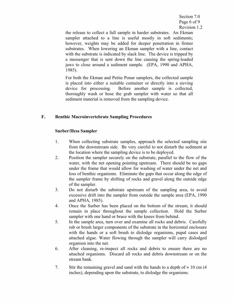
Section 7.0 Page 6 of 9 Revision 1.2
the release to collect a full sample in harder substrates. An Ekman sampler attached to a line is useful mostly in soft sediments; however, weights may be added for deeper penetration in firmer substrates. When lowering an Ekman sampler with a line, contact with the substrate is indicated by slack line. The device is tripped by a messenger that is sent down the line causing the spring-loaded jaws to close around a sediment sample. (EPA, 1990 and APHA, 1985).
For both the Ekman and Petite Ponar samplers, the collected sample is placed into either a suitable container or directly into a sieving device for processing. Before another sample is collected, thoroughly wash or hose the grab sampler with water so that all sediment material is removed from the sampling device.
F. Benthic Macroinvertebrate Sampling Procedures
Surber/Hess Sampler
1. When collecting substrate samples, approach the selected sampling site from the downstream side. Be very careful to not disturb the sediment at the location where the sampling device is to be deployed.
2. Position the sampler securely on the substrate, parallel to the flow of the water, with the net opening pointing upstream. There should be no gaps under the frame that would allow for washing of water under the net and loss of benthic organisms. Eliminate the gaps that occur along the edge of the sampler frame by shifting of rocks and gravel along the outside edge of the sampler.
3. Do not disturb the substrate upstream of the sampling area, to avoid excessive drift into the sampler from outside the sample area (EPA, 1990 and APHA, 1985).
4. Once the Surber has been placed on the bottom of the stream, it should remain in place throughout the sample collection. Hold the Surber sampler with one hand or brace with the knees from behind.
5. In the sample area, turn over and examine all rocks and debris. Carefully rub or brush larger components of the substrate in the horizontal enclosure with the hands or a soft brush to dislodge organisms, pupal cases and attached algae. Water flowing through the sampler will carry dislodged organism into the net.
6. After cleaning, re-inspect all rocks and debris to ensure there are no attached organisms. Discard all rocks and debris downstream or on the stream bank.
7. Stir the remaining gravel and sand with the hands to a depth of ≈ 10 cm (4 inches), depending upon the substrate, to dislodge the organisms.

Section 7.0 Page 7 of 9 Revision 1.2
8. Examine two to three handfuls of substrate to confirm that all organisms have been removed (King, 1993).
9. During sampling, monitor the net for excess sediment and/or detritus (algae, leaves, plant material, etc.) retained in the sampler. Excess material may result in the net clogging and backwashing, greatly reducing the effectiveness of the sampler.
10. When the net appears to be clogged, remove and inspect the larger pieces of detritus. When the inspected material is free from organisms, discard the material downstream.
11. When the sub-sample is completed, hold the net upright, splash water on the outside of the net to wash organisms and detritus to the bottom of the net/bucket.
12. Holding the net over a sieve, unscrew the bucket from the bottom of the net. Using undisturbed stream water, rinse the contents of the bucket and net into the sieve (500 µm). Examine the Surber/Hess bucket and net to ensure the removal of all organisms.
13. When the sampling device only has a net, rinse the contents of the net to the bottom and grasp the net just above the top of the debris. Hold the net over a sieve or shaker/rocker and turn the net inside out. Release the net and rinse the contents of the net into the sieve or shaker/rocker using undisturbed stream water or water previously filtered through the sieve or shaker rocker. Examine the net to ensure the removal of all organisms.
14. If the samples have been collected in the sample bucket or placed within the shaker, the composited sample can be cleaned in a shaker/rocker or sieve to remove most of the fine sediment.
a. Continue to use the shaker/rocker or sieve until as much of the fine
sediment is removed as practicle. Gently force the sample contents down to the center of the bottom of the shaker where the sliding door is located.
b. Put a jar underneath this door and slide the screen opening allowing the sample material to fall into the sampling jar. Carefully rinse the remains in the shaker into the jar with some of the water that has been strained through a 500 µm aperture diameter net.
c. Visually inspect the shaker to ensure removal of all organisms.
15. Empty the contents of the sieve into a pre-labeled sample jar (internal label (rag bond paper in pencil) and external label). Each sample label will include the following:

Section 7.0 Page 8 of 9 Revision 1.2
a. Sample identification number (unique) b. Sample or tributary location c. Date d. Time e. Name of field sampler (s) f. Multiple jars (1of 2, 2of2, etc.)
16. Fill the sample jar (ensuring all sample material is covered) with
preservative (95% ethanol), clean the lid and top of the sample jar and seal.
17. Repeat preceding procedures on remaining sub-samples.
Ponar/Ekman Sampling
Ponar/Ekman (standard or Petite) samplers are used in benthic macroinvertebrate assessments and surveys to study the depositional community. One Ponar/Ekman sample will be collected at each site. The sample will consist of three Ponar/Ekman grab samples. Samples will be taken from depositional/slack water areas within the sampling site. 1. When collecting benthic samples, approach the selected site from
downstream side. Be very careful not to disturb the sediment at the location where the sampling device is to be dropped.
2. If the depth of the sampling location requires the use of a boat, the boat will have to be manipulated in such a way as to allow the proper sampling techniques for the Ponar or Ekman to be employed.
3. Once the location has been approached, slowly lower the Ekman or Ponar to the substrate to reduce the effect of the shock wave produced as the instrument hits the sediment.
4. Once the sampling device reaches the bottom, activate the release as soon as possible and slowly bring the unit back to the surface with the sample.
5. Place the sample into a sampling bucket. After dumping the sample into the sampling bucket inspect the inside of the Ponar/Ekman to ensure that the entire sample has been released from the sampling device.
a. If some substrate remains stuck to the sampler, place the sampler
in a clean bucket or tub. b. Use a wash bottle filled with undisturbed stream water, tap water,
or distilled water to spray the substrate off of the sampler 6. Repeat steps “3.”, “4.” and “5.” until sample collection (total: 3 grabs) is
complete. 7. After sample collection is complete, transfer a manageable amount of the
sample into a 500 µm standard testing sieve. Rinse, decant and empty the contents of the sieve into a pre-labeled sample jar(s).

Section 7.0 Page 9 of 9 Revision 1.2
8. Empty the contents of the sieve into a pre-labeled sample jar (internal label (rag bond paper in pencil) and external label). Each sample label will include the following:
a. Sample identification number (unique) b. Sample or tributary location c. Date d. Time e. Name of field sampler (s) f. Multiple jars (1of 2, 2of2, etc.)
9. Repeat step “8” on the remaining sample material until the entire sample is sieved.
10. Fill the sample jar(s) (ensuring all sample material is covered) with preservative (95% ethanol), clean the lid and top of the sample jar and seal.
G. Quality Assurance/Quality Control Procedures (QA/QC)
Follow all QA/QC procedures in Section 5.0

Section 8.0 Page 1 of 3 Revision 1.2
8.0 PROCEDURE TO ESTABLISH AND USE PHOTO POINTS
The photo point is a method of monitoring that provides a way to assess changes to a point of reference or a landscape view over time. Photographs or digital images taken from the same vantage point at a planned frequency provide a visual record that may be more easily understood by the non-scientific community than detailed quantitative analysis. These photographs or digital images also provide valuable supplementary information for detailed scientific studies.
A. Photo Point Location
The photo point needs to be located in a manner that assures that the point can be relocated in the field at a latter date. A permanent marker such as a piece of rebar, an old disk blade, an embedded set of bricks or a concrete block should be placed at the photo point and used as a reference for taking photos. The marker needs to be further identified by painting with fluorescent paint, use of a flag, reference stake or steel post to help in relocating. Locating with a Global Positioning System (GPS) is also advised. Care should be taken when setting the point to account for livestock or other potential disturbances to the marker and use common sense in choosing the type of marker to be placed. The marker should be undisturbed throughout the project duration and it may be advantageous to leave a marker permanently in anticipation of future use in monitoring follow-up. The photo point should be located on a map preferably an aerial photo. The map can be taken to the field and used as a guide in finding the marker. Using the GPS is also useful in relocating the point. GPS location data (latitude and longitude) should be a part of the map description as well as Township, Range and Section. It is also recommended to provide a written description of the photo point with reference to any obvious identifying characteristics such as a lone tree, fence posts, a particular-looking rock, etc.
B. Equipment The only equipment needed for this procedure is a camera, a pencil and a notepad. The camera may be conventional or digital with sufficient quality to take clear photographs or images of the item of interest. The same camera or one with similar attributes should be used throughout the project.

Section 8.0 Page 2 of 3 Revision 1.2
C. Photo Point Procedure
The photographer should initially note the date, general weather conditions, and time of day. A brief written description of the item to be photographed should be included on the notepad and developed for each photograph taken. Note the photo or image number with each description so one can identify the images or prints after they are developed. One should try to take the photographs at the same time of day, in similar light, similar weather conditions and at the same season of the year. Stand adjacent to the photo point in the same manner each time and note the direction you are facing. When taking the photograph, you should be aware of and account for your shadow or other disturbances that may detract or obscure the interpretation of the picture or image. Look through the camera at the item of interest and see if there is anything within the camera field that can be used as a reference point for future photographers. Is there a tree or skyline feature in the viewfinder that will help locate the photo point? These features should be described in sufficient detail to enable a photographer to view these references with relative ease during photograph sessions. If no obvious reference points are within the field of view, you either can use compass bearings, or, an artificial reference point can be placed within the field of view. Remember to take into account potential disturbances to the marker from livestock or other potential problems. A minimum of two photographs per item should be taken and their descriptions logged onto the notepad. Additional photographs may be taken at different angles or views at the discretion of the photographer to further document the point. Photo sessions should be conducted at time intervals that allow for anticipated changes to the items of interest and should coincide with other assessments of the item of interest. Project progress, time of season, budgetary constraints, etc. should be considered when choosing photo session frequency.
D. Photo Point Data Management
Once the photographs or images are developed, the photos or images with written descriptions should be placed in a binder or other record book or file. The negatives should be accompanied by written descriptions and placed in appropriate storage. Working copies of the photographs should be made available to facilitate future photo sessions at the site and provide information and education for the project.

Section 8.0 Page 3 of 3 Revision 1.2
E. Photo Point Interpretation
A picture can be worth a thousand words and the photo point procedure can provide just that if it is done properly. The procedure is meant to provide a visual record of the changes (or lack of changes) of an item of interest. It may be necessary sometimes to provide the viewer with a description of what they are seeing and why the photographs are different. This is when the writer supports the photograph with written descriptions that direct the viewer to particular items in the photographs. Once this is accomplished, the viewer can then make interpretations of what he/she sees in the pictures.
Section 9.0 Page 1 of 41 Revision 1.2
9.0 PHYSICAL HABITAT CHARACTERIZATION
A. Introduction
Assessing the aquatic habitat provides information on the condition or availability of habitat within a reach of river/stream. In conjunction with water chemistry, stream flow gauging, fish and macroinvertebrate sampling, an overall picture of the condition or health of a river or stream can be discerned. The methods described in this protocol can provide comparable data regarding the physical, chemical, and biological health of a river/stream and help to understand the stream dynamics and relationship to the populations of fish and macroinvertebrates within a stream. The South Dakota Department of Environment and Natural Resources, Water Resources Assistance Program (SDDENR-WRAP) uses a habitat assessment protocol based on research conducted by South Dakota State University (SDSU). The focus of that research was to determine if rivers within South Dakota exhibit longitudinal trends with regard to physical habitat and fish communities (Milewski 2001). A secondary goal was to determine which physical habitat variables have the most influence on the distribution of the fish communities.
The physical habitat assessment methods used in the SDSU investigation were adapted from Simonson et al. (1994), Platts et al. (1983) and Frissell et al. (1986) (Milweski 2001). The SDSU investigation using these methods focused on two major rivers within South Dakota. Data was collected from the Bad River in the Northwestern Great Plains ecoregion and the Big Sioux River in the Northern Glaciated Plains ecoregion. The habitat assessment protocols used by the SDSU study and described in this document were an effective assessment tool for quantifying the physical differences that exist along the longitudinal gradient of the rivers in South Dakota. River reaches were selected within one type of riparian land use in most cases, and where bridges and dams appeared to have minimal impact. This methodology is similar to other habitat assessment methods which use transect data to assess a reach of stream or river, such as the Environmental Monitoring and Assessment Program (EMAP): Western Pilot Study. Transect data collection is divided into three practical components based on tools used. The first suite of data is collected according to visual estimates and counts. On either end of a transect the riparian land use, dominant vegetation type, animal vegetation use, dominant bank substrate, and bank slumping (presence/absence) are recorded. Where a transect crossed the stream, dominant macrohabitat type is designated as pool, riffle, or run. Bed substrate data is collected using the Wolman “pebble count” by visually dividing the transect into eight “cells”. Within each cell, substrate size is measured and the class size recorded. This method, which objectively classifies substrates in clear streams, is a necessity in turbid streams where visual estimates are not possible.

Section 9.0 Page 2 of 41 Revision 1.2
A second suite of data focuses on stream bank and riparian features that are measured with a graduated pole and angle finder. After identifying the break point between the channel bank and channel bottom, measurements related to stream bank length, bank angle, and bank height are taken (Figure 9.0.12). Along the stream bank length, the length of bank that was vegetated, eroded, and/or depositional was measured. The vegetated portion is the length of bank where root structure contributed to bank stability, eroded portions is that length with no root structure support, and a depositional portion is that length where recent deposition dominates the bank surface. Riparian-related cover types are measured at the end of each transect as the horizontal length of overhanging vegetation (OHV) and undercut bank (UCB) extending over the streambed. A third suite of data focuses on horizontal and vertical point measurements which are used to calculate stream width, depth and velocity; channel bottom and top width; and bankfull width, depth, and width:depth ratio. At most sites, point data will be obtained by staking a tape measure from left top bank to the right top bank. In some cases, the tape measure can be staked at left bankfull and right bankfull. Moving from left to right, key channel features (i.e., location codes) are identified and the distance from the left stake is recorded. Vertical measurements are bankfull depth, water depth, and water velocity. Bankfull depths are measured at water edge and at three points within the stream. Water depth and velocity are measured at the three points within the stream (1/4, 1/2, and 3/4 of the distance across the stream surface). At each site, data are also collected on large woody debris (LWD), discharge, water surface slope, and water quality. The number of LWD is tallied for the entire reach according to methods designed by Robison and Beschta (1990). Length and diameter of all LWD are measured and can be used to calculate the volume of LWD within the reach. Discharge data is collected at a single transect or other stream cross-sections where flow is uniform. The velocity-area method described in the SDDENR-WRAP standard operation procedures manual is used. Water surface slope (%) is calculated by dividing the drop in water surface from transect one to transect 11 by the longitudinal stream distance using a surveying level. Physicochemical water quality data collected is water temperature, air temperature, turbidity, dissolved oxygen, and conductivity. These measurements are also made twice at each reach, once at the beginning of the assessment and a second time when all other physical habitat measurements have been collected, due to the length of time it takes to complete the assessment for one site. A standard chemical sample (nutrients, bacteria, and solids) can be collected during the habitat assessment. Standard operating protocols for this sampling are presented in the SD DENR-WRAP SOP (Volume I, Tributary Sampling (12.0)). Most water quality sampling sites for the South Dakota Water Resources Assistance Program are at locations where permission is not needed to access the sites. However, the reach selection for the habitat and physical assessment will

Section 9.0 Page 3 of 41 Revision 1.2
be performed over a considerable distance (≈35X the stream width) so it may be necessary to gain permission from the land owners depending on the location of some sites within the sampling reach. The flow chart on the following page shows the groups of parameters and how they should be collected in relation to one another, i.e. workflow (Figure 9.0.1). The chemistry, hydrology, and biological data including chlorophyll a and periphyton communities will be integrated to determine, in relation to similar sites located in the same ecoregion, what cause and effect relationships may exist between the physical, chemical, and biological data.
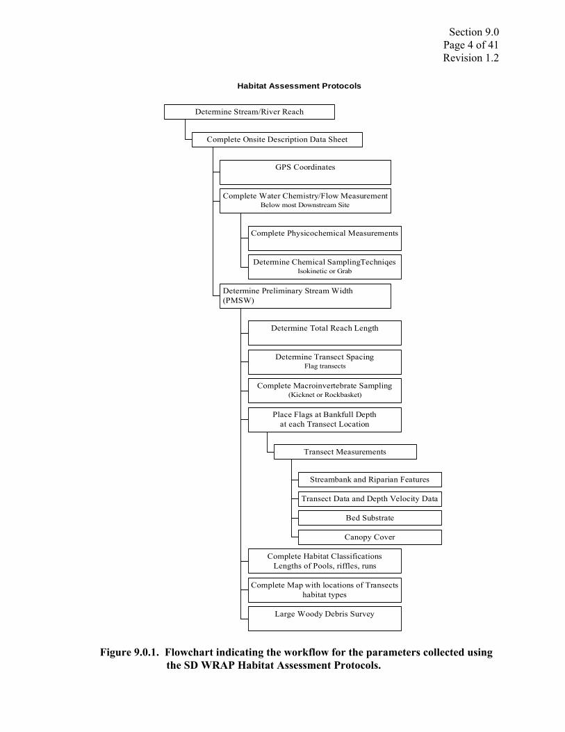
Section 9.0 Page 4 of 41 Revision 1.2
Habitat Assessment Protocols
GPS Coordinates
Complete Physicochemical Measurements
Determine Chemical SamplingTechniqesIsokinetic or Grab
Complete Water Chemistry/Flow MeasurementBelow most Downstream Site
Determine Total Reach Length
Determine Transect SpacingFlag transects
Complete Macroinvertebrate Sampling(Kicknet or Rockbasket)
Streambank and Riparian Features
Transect Data and Depth Velocity Data
Bed Substrate
Canopy Cover
Transect Measurements
Place Flags at Bankfull Depthat each Transect Location
Complete Habitat ClassificationsLengths of Pools, riffles, runs
Complete Map with locations of Transectshabitat types
Large Woody Debris Survey
Determine Preliminary Stream Width(PMSW)
Complete Onsite Description Data Sheet
Determine Stream/River Reach
Figure 9.0.1. Flowchart indicating the workflow for the parameters collected using the SD WRAP Habitat Assessment Protocols.

Section 9.0 Page 5 of 41 Revision 1.2
B. Data Collection Procedures
1. Reach Selection
Most water quality monitoring sites for the South Dakota Water Resources Assistance Program (SD WRAP) are positioned at locations where permission is not needed to access the site (Right-of-way) and are outlined in the Project Implementation Plan (PIP). However, reaches should be selected either upstream or downstream of a bridge or culvert if one is present. The distance upstream or downstream of a channel modification should be long enough so that there is minimal influence on channel morphology and/or the riparian zone. Some general guidelines that should be considered when selecting the sampling reach are: • Reaches should exhibit only one type of landuse outside of the
riparian zone. A mix of CRP and heavily grazed land should be avoided.
• Minimal influence due to bridges, culverts or dams • The entire reach should be inspected to determine any problems
with site prior to sampling • If at all possible, dams, bridge abutments, and other water control
structures/obstructions should not be present within the stream length.
• Get Permission from the landowner(s). 2. On-Site Description Data Sheet - (Section A)
After selecting a suitable reach for the habitat assessment, On-Site Description Data Sheet (Section A) should be completed. This includes the following: • Project Site ID, i.e. nearest monitoring station for assessment • Stream Name • Locational information (Township, Range, Section, GPS
coordinates, etc). • Investigators’ Names • Date and Time
Section A Project Site ID: Date: Stream Name:
T , R , 1/4 of Sec______ Time:
Transect 1(Upstream) Transect 11(Downstream) GPS Coordinates (utm): Northing: Easting: Northing: Easting:
Investigators:

Section 9.0 Page 6 of 41 Revision 1.2
3. Preliminary Mean Stream Width (PMSW) - (1.1 Section B)
After a suitable sampling reach has been located the PMSW needs to be calculated and used to determine transect spacing (Simonson et al. 1994). Measure the wetted width of the stream in approximately 5 to 10 locations at various points along the tentative reach length. When low flows restrict stream width to a small portion of the streambed or the streambed is dry, streambed width is used to calculate the PMSW. Within each reach 11 transects are placed 3 PMSWs apart (Figure 9.0.2). According to the SDSU investigation, in most cases, prairie streams within South Dakota greater than 10 m (32.8 feet) wide can be homogenous (e.g., uniform in channel morphometry and depth), and transects spaced 3 PMSWs were judged to be adequate. However, data on the lower 4 reaches of the Big Sioux River indicated that transects spaced 2 PMSW were relatively homogenous in relation to channel morphometry and depth. As a result, watersheds greater than 500 km2 (193.1 mi2) and wider than 10m (32.8 feet) will have transects spaced 2 PMSW apart. According to Simonson et al. (1994) the wetted width is defined as the wetted surface of the stream excluding islands, exposed bars, backwaters, and adjacent wetlands, measured from one bank to the other, perpendicular to the direction of the stream flow. Note: After the PMSW has been calculated and transect locations determined, the next step in the assessment should be to collect macroinvertebrate samples prior to any more disturbances of the site. When calculating the mean stream width the following should be considered: • Mean stream widths should be determined at or near base flow
conditions. • When low flows restricted stream width to a small portion of the
streambed, streambed width should be used to determine transect spacing.
• According to Simonson et al. (1994) streams with a PMSW of < 3m should have a sampling reach of at least 100m.
• After progressing downstream for the associated reach and taking the necessary width measurements, calculate the average to determine the PMSW. Round the PMSW to the nearest 0.1m.
• Distances between transects are measured from the center of each transect in the stream.

Section 9.0 Page 7 of 41 Revision 1.2
Section B
Preliminary Mean Stream Width (PMSW) Width Number
1 2 3 4 5 6 7 8 9 10 Sum Avg. PMSW
Width (0.1m) Transect Spacing *: *If PMSW <10m space transects every 3 PMSW. If >10m, transects are spaced every 2 PMSW. Total Reach Length: Reach Length = 11 Transects, 10 distances apart X 3 PMSW = 30 PMSW or 20 PMSW if width >10m.
Transect Spacing
Transects are marked with flags, then data collection begins on the upstream end of the reach proceeding downstream. Left bank and right bank are determined as you look downstream.
Transect Spacing
3 mean stream widths between transects
If mean stream width >10mthen 2 mean stream widthsbetween transects
1
2 3
4 5 6 7
8 9
10 11
Figure 9.0.2. Transect Spacing (Milewski 2001).

Section 9.0 Page 8 of 41 Revision 1.2
a. If the PMSW is <10m, eleven transects will be spaced three
PMSW apart. The number of transects is dependent upon the PMSW calculated above.
b. Within each reach (station), transects are spaced approximately every three times the PMSW.
c. According to Milewski (2001) most streams greater than 10 m wide are homogenous in various habitat measurements, i.e. depth and channel morphometry.
d. On larger streams greater than 10m, since there is such a large distance between transects, the distance is dropped to 2 PMSWs between sampling locations.
e. Eleven transects will be collected for each reach. f. Transects are established every two to three times the PMSW
depending on the PMSW, perpendicular to stream flow, with the first transect located one-half PMSW upstream from the downstream end of the station (Simonson et al., 1994).
g. Distances between transects are measured from the bank and are perpendicular to the current/streambank.
h. Eleven transects are spaced evenly resulting in 30 mean stream widths (msw) for the entire reach length.
i. Flag transects on either side of the stream and locate the distance on the data sheet, On-Site Description Data Sheet (Section B).
j. After flagging the location of the transects, chemical sampling should be initiated at this time if required by the PIP (SD WRAP Volume I Section.12.0). After chemical sampling is complete, macroinvertebrate samples should be collected using methods outlined in SD WRAP Volume II Section 6.0 prior to anymore disturbance of the site.
4. Water Chemistry - (Section C)
If chemical sampling is part of the overall sampling regime during the habitat assessment, this should occur during the preliminary stages of setup prior to any disturbance of the site. Samples should be collected at the most upstream transect of the sampling reach to minimize the impact from setting up the reach for transect data collection.
If a stream sample is to be collected, the method described in SD WRAP Volume I Section 12.0, Tributary Sampling Techniques, should be followed. The depth and velocity will dictate which sampling equipment will need to be used, i.e. integrated sediment sampler (isokinetic) vs. grab sampling method. The water quality sample should be collected at the same location as the discharge measurement.
Section C of the datasheet should be filled out twice during the day. In many instances the water chemistry will change during the course of the

Section 9.0 Page 9 of 41 Revision 1.2
day. Once in the morning upon arrival and once more at the end of the work period at the same location within the reach.
Section C
Water Quality
Reading
Time (2400)
Water Temperature
(oC)
Air Temperature
(oC)
Turbidity
(NTU)
Secchi (cm)
Dissolved Oxygen (mg/L)
Specific Conductance
(µS/cm)
Conductivity
(µS/cm)
Morning Afternoon
Visual Observations 1) Odor
(Severe, Extreme, Moderate, Mild, None)
2) Septic (Severe, Extreme, Moderate,
Mild, None)
3) Deadfish (Severe, Extreme, Moderate,
Mild, None)
4) Surface Film (Severe, Extreme, Moderate,
Mild, None) 5) Color: 6) Ice Cover (Severe, Extreme, Moderate, Mild, None)
Weather Conditions:
Current
Past 24 hrs
Field Comments:
Clear/sunny Partly cloudy
Intermittent showers Steady rain Heavy rain
5. Stream Discharge - (Section K)
Figure 9.0.3. Discharge Measurement Methods (Peck, et al. 2001).

Section 9.0 Page 10 of 41 Revision 1.2
Flow should also be collected at this time at the upstream site. It is important to choose a channel cross section that is as much like a canal as possible. A glide area with a “U” shaped channel cross section that is free of obstructions provides the best conditions for measuring discharge by the velocity-area method (see Figure 6-1 taken from EMAP Field Methods Manual, April 2001). In the method, the discharge is collected at 0.6 depth or 0.2/0.8 depth of the channel depending on the total depth of the channel (according to USGS methods and SD WRAP- Volume I SOP).
a. Rocks and other obstructions should be removed from the cross-
section prior to any measurement. The procedure for discharge measurements (depth and velocity measurements) is outlined in SDWRAP-SOP Method in Volume I (SD DENR-SOP).
b. EMAP protocols state that in channels too small for the velocity-area method, discharge can sometimes be determined directly by measuring the time it takes to fill a container of known volume. ‘Small’ is defined as a channel so shallow that the current velocity probe (or pygmy meter) cannot be placed in the water, or where the channel is irregular due to rocks and debris, and suitable cross-section for using the velocity area procedure is not available. If obtaining data by this procedure will result in substantial channel disturbance, wait until all other activities (biological and chemical) have been completed (Peck et al. 2001).
c. A data page for collection of the discharge data is available in Appendix D, Section K, of this document. This is part of the onsite data which needs to be collected only once. The full set of datasheets is included in Appendix A of this document.
6. Habitat Classification - (Section D)
Once the PMSW has been determined and the transects have been located along the reach, one person should be sampling macroinvertebrates and the second field technician should be determining the number of different habitat types found within the reach. As you start a new segment, estimate the number of habitats by documenting them in Section D of the on-site description data sheet and locate them on the map in Section E (Map, Slope Measurement and Photo Documentation Data Sheet). Locate the riffles to the nearest transect and number. Also locate the riffles by transect and estimate their length within the entire stream reach.

Section 9.0 Page 11 of 41 Revision 1.2
Section D
Habitats Available number of each (also place on map Section E)
Pool Run/Glide Riffle Other (describe) _________. (Table 9.0.1) Lengths of Riffle(s): , , , , . (meters) Nearest Transect # : , , , , . Total Length (riffles) =___________ Pool Forming Elements = ___________ (Table 9.0.1)
a. After measuring the reach quickly estimate the number of general
habitats found within the reach. This includes pools, runs, riffles, and others. For each riffle or other unique habitat type, estimate the length and locate it to the nearest transect number. Use EMAP definitions (Table 9.0.1).
• This is done for the entire reach. When you draw out your
map, you should describe the habitat between transects and document any riffles (thus, you should come up with a continuous map of the reach). Within the reach you measure every riffle and document where pools and runs are. Then count up the number of riffles and/or pools and/or runs. The total length is the total length of all the riffles you measured.
b. Identify the habitat type on the map to the nearest upstream or
downstream transect (EMAP definition – Table 8.0.1). Before being considered large enough to be identified as a channel-unit scale habitat feature, the unit should be at least as long as the channel is wide. For instance, if there is a small, deep (pool-lie) area at the thalweg within a large riffle area, don’t record it as a pool unless it occupies an area about as wide or long as the channel is wide. These channel unit habitat classifications and pool-forming elements are modified from those of Bisson et al. (1982) and Frissell et al. (1986). The channel habitat types in Table 9.0.1 were developed specifically for salmonid streams.

Section 9.0 Page 12 of 41 Revision 1.2
Table 9.0.1. Channel unit and Pool Forming element categories.
Channel Unit Habitat Classesa
Class (Code) Description Pools: Still water, low velocity, smooth, glassy surface, usually deep
compared to other parts of the channel: Plunge Pool (PP) Pool at base of plunging cascade or falls. Trench Pool (PT) Pool-like trench in the center of the stream. Lateral Scour Pool (PL) Pool scoured along a bank. Backwater Pool (PB) Pool separated from main flow off the side of the channel. Impoundment Pool (PD) Pool formed by impoundment above dam or constriction. Pool (P) Pool (unspecified type).
Glide (GL) Water moving slowly, with a smooth, unbroken surface. Low turbulence.
Riffle (RI) Water moving, with small ripples, waves and eddies -- waves not breaking, surface tension not broken. Sound: "babbling", "gurgling".
Rapid (RA) Water movement rapid and turbulent, surface with intermittent whitewater with breaking waves. Sound: continuous rushing, but not as loud as cascade.
Cascade (CA) Water movement rapid and very turbulent over steep channel bottom. Most of the water surface is broken in short, irregular plunges, mostly whitewater. Sound: roaring.
Falls (FA) Free falling water over a vertical or near vertical drop into plunge, water turbulent and white over high falls. Sound: from splash to roar.
Dry Channel (DR) No water in the channel aNote that in order for a channel habitat unit to be distinguished, it must be at least as wide or long as the channel is wide.
Categories of Pool-forming Elements (Taken from Peck, et.al, 2001)b
Code Category N Not Applicable, Habitat Unit is not a pool W Large Woody Debris R Rootwad B Boulder or Bedrock F Unknown cause (unseen fluvial processes) WR, RW, RBW Combinations OT Other (describe in the comments section of field form) b Remember that most pools are formed at high flows, so you may need to look at features, such as large woody debris, that are dry at baseflow, but still within the bankfull channel.
Classify the appropriate habitat type and determine its length and position (nearest transect) within the entire sampling reach.

Section 9.0 Page 13 of 41 Revision 1.2
7. Map, Slope Measurements, and Photo Documentation Data Sheet -
(Section E)
After each transect has been flagged, the water quality, discharge data, and macroinvertebrate samples have been collected, the water surface slope can be determined. This measurement can also wait until all other data have been collected. Water surface slope (%) is calculated by dividing the drop in water surface from transect one to transect eleven by the longitudinal stream distance using a surveying level. To determine slope on tributaries you can use the level instrument. For larger rivers, i.e. Cheyenne, Bad, and the Big Sioux, slope can easily be collected from the topography maps. Tributaries are defined as having a drainage area of less than 500 km2. Anything greater than 500 km2 is considered a large river (Milewski 2002). This is primarily done to save time as collecting water surface slope measurements for a reach on a large river can take a considerable amount of time.
a. Map, Slope Measurements, and Photo Documentation Data should
be collected in the field for each site. The water surface slope in field should be collected for tributaries that have a drainage area of less than 500 km2 (123,553 acres) or 193.1 mi2.
b. If the drainage area is greater than 500 km2 then the slope should be taken from the topography maps. Collecting slope information on large river systems takes a tremendous amount of time and the data can be taken from topography maps with a fair amount of accuracy.
c. If the drainage area is less than 500 km2 then the slope should be derived in the field using the following procedure and datasheet in Section E of the datasheet section and listed here.
Section E
Water Surface Slope Measurements for Reach if drainage area smaller than 500km2
Transect #
Height of Inst.
(cm)
Rod Reading from water surface (cm)
Elevation Difference (0.01 m)
Horizontal Distance (reach length above)
Slope (m/m)
Slope (%)
d. Place the instrument at a location near the Transect 5-6 or in a
position where the rod can seen at both Transect 1 and 11. Begin with the first transect and shoot the change in slope from the beginning transect to the next transect (if necessary). If at all possible, simply shoot both the furthest downstream and upstream

Section 9.0 Page 14 of 41 Revision 1.2
transects (1 and 11) from the same location. Water surface slope should be placed in the Section E data sheet.
Draw a map of the site with location of most upstream and most downstream transects. Include locations of photographic points, direction of photograph, and frame number.
Approximate Distance
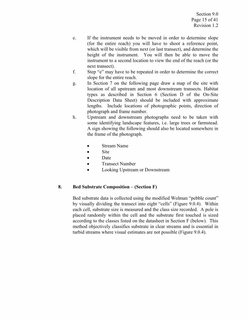
Section 9.0 Page 15 of 41 Revision 1.2
e. If the instrument needs to be moved in order to determine slope
(for the entire reach) you will have to shoot a reference point, which will be visible from next (or last transect), and determine the height of the instrument. You will then be able to move the instrument to a second location to view the end of the reach (or the next transect).
f. Step “e” may have to be repeated in order to determine the correct slope for the entire reach.
g. In Section 7 on the following page draw a map of the site with location of all upstream and most downstream transects. Habitat types as described in Section 6 (Section D of the On-Site Description Data Sheet) should be included with approximate lengths. Include locations of photographic points, direction of photograph and frame number.
h. Upstream and downstream photographs need to be taken with some identifying landscape features, i.e. large trees or farmstead. A sign showing the following should also be located somewhere in the frame of the photograph. • Stream Name • Site • Date • Transect Number • Looking Upstream or Downstream
8. Bed Substrate Composition – (Section F)
Bed substrate data is collected using the modified Wolman “pebble count” by visually dividing the transect into eight “cells” (Figure 9.0.4). Within each cell, substrate size is measured and the class size recorded. A pole is placed randomly within the cell and the substrate first touched is sized according to the classes listed on the datasheet in Section F (below). This method objectively classifies substrate in clear streams and is essential in turbid streams where visual estimates are not possible (Figure 9.0.4).
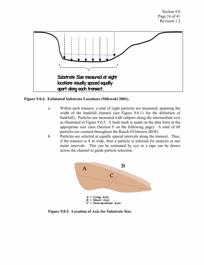
Section 9.0 Page 16 of 41 Revision 1.2
Substrate Size measured at eightlocations visually spaced equally apart along each transect.
Figure 9.0.4. Estimated Substrate Locations (Milewski 2001).
a. Within each transect, a total of eight particles are measured, spanning the width of the bankfull channel (see Figure 9.0.11 for the definition of bankfull). Particles are measured with calipers along the intermediate axis as illustrated in Figure 9.0.5. A hash mark is made on the data form in the appropriate size class (Section F on the following page). A total of 88 particles are counted throughout the Reach Of Interest (ROI).
b. Particles are selected at equally spaced intervals along the transect. Thus, if the transect is 8 m wide, then a particle is selected for analysis at one meter intervals. This can be estimated by eye or a tape can be drawn across the channel to guide particle selection.
Figure 9.0.5. Location of Axis for Substrate Size.
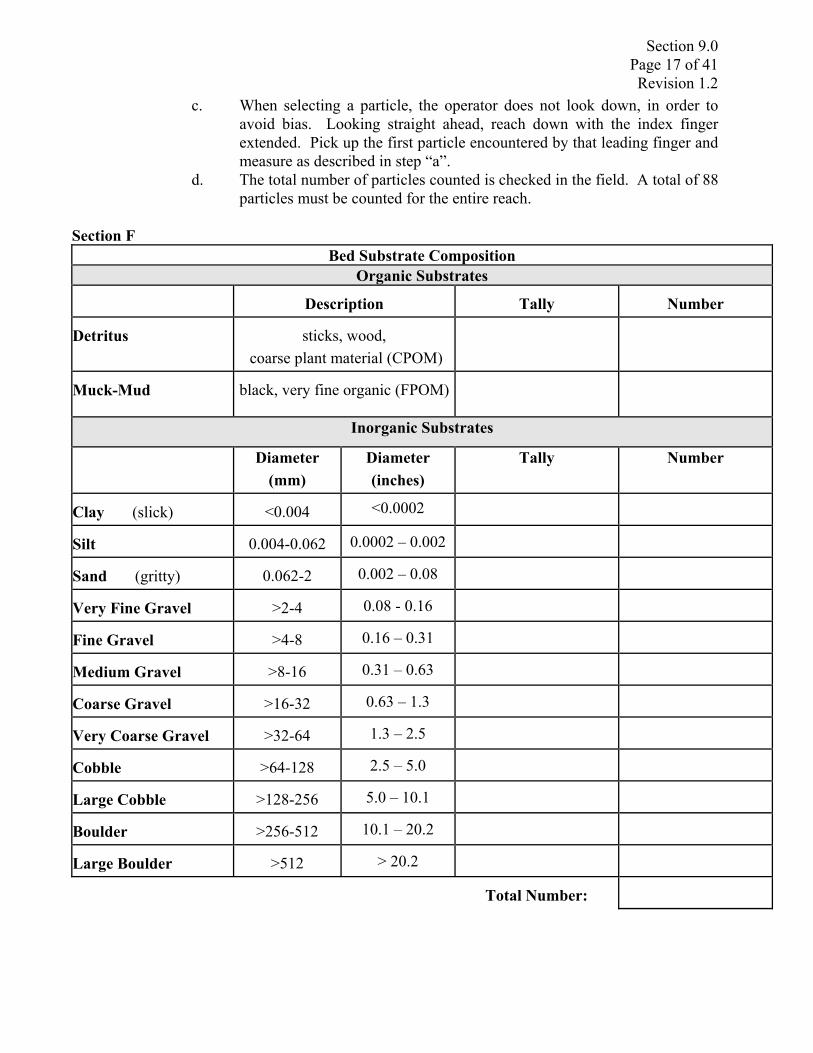
Section 9.0 Page 17 of 41 Revision 1.2
c. When selecting a particle, the operator does not look down, in order to avoid bias. Looking straight ahead, reach down with the index finger extended. Pick up the first particle encountered by that leading finger and measure as described in step “a”.
d. The total number of particles counted is checked in the field. A total of 88 particles must be counted for the entire reach.
Section F
Bed Substrate Composition Organic Substrates
Description
Tally
Number
Detritus
sticks, wood,
coarse plant material (CPOM)
Muck-Mud
black, very fine organic (FPOM)
Inorganic Substrates
Diameter (mm)
Diameter (inches)
Tally Number
Clay (slick)
<0.004 <0.0002
Silt
0.004-0.062 0.0002 – 0.002
Sand (gritty)
0.062-2 0.002 – 0.08
Very Fine Gravel
>2-4 0.08 - 0.16
Fine Gravel
>4-8 0.16 – 0.31
Medium Gravel
>8-16 0.31 – 0.63
Coarse Gravel
>16-32 0.63 – 1.3
Very Coarse Gravel
>32-64 1.3 – 2.5
Cobble
>64-128 2.5 – 5.0
Large Cobble
>128-256 5.0 – 10.1
Boulder
>256-512 10.1 – 20.2
Large Boulder
>512 > 20.2
Total Number:

Section 9.0 Page 18 of 41 Revision 1.2
9. Large Woody Debris Tally – (Section G)
Methods for Large Woody Debris (LWD) measurement were adapted from Robison and Beschta (1990). Both the EMAP Physical Habitat Characterization and methods used be Milewski (2001) allow quantitative estimates of the number, size, total volume and distribution of wood within the stream reach. LWD is defined as woody material with a small end diameter of at least 10cm (4 in.) and a length of at least 1.5 m (5 ft.) (Peck et al., 2001).
The procedure for tallying LWD is presented in the following bulleted section. The tally includes all pieces of LWD that are at least partially in the baseflow channel, the “active channel” (flood channel up to bankfull stage), or spanning above the active channel (Figure 11). The active (or “bankfull”) channel is defined as the channel that is filled by moderate-sized flood events that typically recur every one to two years. LWD in the active channel is tallied over the entire length of the reach, including the area between the channel cross-section transects. Pieces of LWD that are not at least partially within Zones 1, 2, or 3 are not tallied.
For each LWD piece, first visually estimate its length and its large and small end diameters in order to place it in one of the diameter and length categories (see below). The diameter class on the datasheet (HA-LWD Form) refers to the large end diameter. Sometimes LWD is not cylindrical, so it has no clear “diameter”. In these cases visually estimate what the diameter would be for a piece of wood with a circular cross section that would have the same volume. When evaluating length, include only the part of the LWD piece that has a diameter greater than 10 cm (4 in). Count each of the LWD pieces as one tally entry and include the whole piece when assessing dimensions, even if part of it is in Zone 4 (outside of the bankfull channel) (Figure 8.0.7). For both the Zone 1-2 wood and the Zone 3 LWD, the field form (Appendix D, Section G) asks for transect spacing (Transects 1-2, 2-3, etc), logjam number (if present), meander location, habitat association, angle (Figure 8.0.7), and the length and diameter of the LWD by using the 12 different categories for tallying debris pieces visually estimated within three length and four diameter class combinations. Each LWD piece is tallied in only one box. There are 12 size classes for wood at least partially in Zones 1 and 2, and 12 for wood partially within Zone 3. Wood that is not at least partially within those zones is not tallied.
a. Procedure for Large Woody Debris Tally
Note: Tally pieces of large woody debris (LWD) within each segment of stream as you complete the densiometer and substrate measurements. Include all pieces whose large end is located within the segment in the tally. When filling out the LWD form
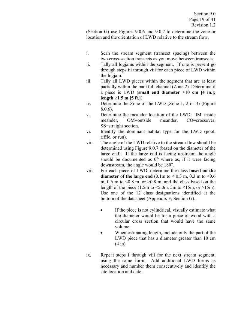
Section 9.0 Page 19 of 41 Revision 1.2
(Section G) use Figures 9.0.6 and 9.0.7 to determine the zone or location and the orientation of LWD relative to the stream flow.
i. Scan the stream segment (transect spacing) between the two cross-section transects as you move between transects.
ii. Tally all logjams within the segment. If one is present go through steps iii through viii for each piece of LWD within the logjam.
iii. Tally all LWD pieces within the segment that are at least partially within the bankfull channel (Zone 2). Determine if a piece is LWD (small end diameter ≥10 cm [4 in.]; length ≥1.5 m [5 ft.])
iv. Determine the Zone of the LWD (Zone 1, 2 or 3) (Figure 8.0.6).
v. Determine the meander location of the LWD: IM=inside meander, OM=outside meander, CO=crossover, SS=straight section.
vi. Identify the dominant habitat type for the LWD (pool, riffle, or run).
vii. The angle of the LWD relative to the stream flow should be determined using Figure 9.0.7 (based on the diameter of the large end). If the large end is facing upstream the angle should be documented as 0o, where as, if it were facing downstream, the angle would be 180o.
viii. For each piece of LWD, determine the class based on the diameter of the large end (0.1m to < 0.3 m, 0.3 m to <0.6 m, 0.6 m to <0.8 m, or >0.8 m, and the class based on the length of the piece (1.5m to <5.0m, 5m to <15m, or >15m). Use one of the 12 class designations identified at the bottom of the datasheet (Appendix F, Section G).
• If the piece is not cylindrical, visually estimate what
the diameter would be for a piece of wood with a circular cross section that would have the same volume.
• When estimating length, include only the part of the LWD piece that has a diameter greater than 10 cm (4 in).
ix. Repeat steps i through viii for the next stream segment,
using the same form. Add additional LWD forms as necessary and number them consecutively and identify the site location and date.
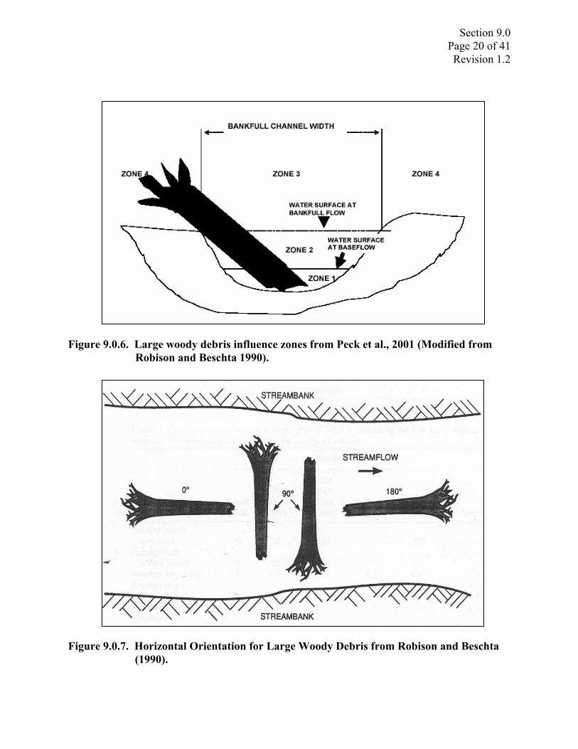
Section 9.0 Page 20 of 41 Revision 1.2
Figure 9.0.6. Large woody debris influence zones from Peck et al., 2001 (Modified from
Robison and Beschta 1990).
Figure 9.0.7. Horizontal Orientation for Large Woody Debris from Robison and Beschta
(1990).

Section 9.0 Page 21 of 41 Revision 1.2
Section G Large Woody Debris Data
Project Site ID:_________________Stream Name:____________Date:_________Page____of____
Transect Spacing
Log Jam Number
LWD
Number
Zone
Meander Location
Habitat
Association
Angle
Length
Diameter
Zone: Zone 1 is water surface at baseflow, Zone 2 is between baseflow surface and bankfull flow surface, Zone 3 is bankfull channel width above bankfull flow surface. Meander Location: IM=inside meander, OM=outside meander, CO=crossover, SS=straight section Habitat Association: PL=pool, RF=riffle, RN=run
LARGE WOODY DEBRIS CATEGORIES (≥10 cm small end diameter; ≥1.5 m length) Categories 1 2 3 4 Diameter Large End 0.1-<0.3m 0.3-0.6m 0.6-0.8m >0.8m Length >1.5-5m 5-15m >15m -

Section 9.0 Page 22 of 41 Revision 1.2
10. Canopy Cover - (Section H)
Riparian canopy cover over a stream is important not only in its role in moderating stream temperatures through shading, but also as an indicator of conditions that control bank stability and the potential for inputs of coarse and fine particulate organic material. Organic inputs from riparian vegetation become food for stream organisms and structure to create and maintain complex channel habitat.
Canopy cover over the stream is determined at each of the 11 cross-section transects. A Convex Spherical Densiometer (model B) is used (Lemmon, 1957). The densiometer must be taped exactly as shown in Figure 9 to limit the number of square grid intersections to 17. Densiometer readings can range from 0 (no canopy cover) to 17 (maximum canopy cover). Six measurements are obtained at each cross-section transect (four measurements in four directions at mid-channel and one at each bank). The mid-channel measurements are used to estimate canopy cover over the channel. The two bank measurements complement your visual estimates of vegetation structure and cover within the riparian zone itself, and are particularly important in wide streams, where riparian canopy may not be detected by the densiometer when standing midstream.
The procedure for obtaining canopy cover data is presented below. Densiometer measurements are taken at 0.3 m (1 ft) above the water surface, rather than at waist level, to (1) avoid errors because people differ in height; (2) avoid errors from standing in water of varying depths; and (3) include low overhanging vegetation more consistently in the estimates of cover. Hold the densiometer level (using the bubble level) 0.3 m above the water surface with your face reflected just below the apex of the taped “V”, as shown in Figure 10. Concentrate on the 17 points of grid intersection on the densiometer that lie within the taped “V”. If the reflection of a tree or high branch or leaf overlies any of the intersection points, that particular intersection is counted as having cover. For each of the six measurement points, record the number of intersection points (maximum=17) that have vegetation covering them in the “Canopy Cover Measurement” section of the form as shown in (Appendix F, Section H).
This method measures canopy cover at 11 evenly spaced transects over a length of stream 30-35 times the channel width with a 100-meter minimum reach length. Six canopy measurements are taken at each transect. Four measurements are taken facing in different directions from the center of the stream and one is taken at each stream bank. It is important to consider the seasonal flow and riparian vegetation conditions when measuring cover using this method since stream widths and deciduous vegetation cover measurements will differ seasonally. Ideally, measurements would be taken during seasonal low flow periods each time to minimize the effects of
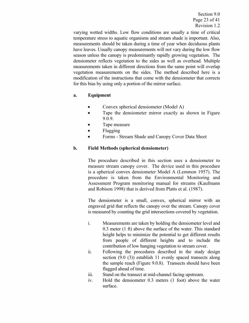
Section 9.0 Page 23 of 41 Revision 1.2
varying wetted widths. Low flow conditions are usually a time of critical temperature stress to aquatic organisms and stream shade is important. Also, measurements should be taken during a time of year when deciduous plants have leaves. Usually canopy measurements will not vary during the low flow season unless the canopy is predominantly rapidly growing vegetation. The densiometer reflects vegetation to the sides as well as overhead. Multiple measurements taken in different directions from the same point will overlap vegetation measurements on the sides. The method described here is a modification of the instructions that come with the densiometer that corrects for this bias by using only a portion of the mirror surface. a. Equipment
• Convex spherical densiometer (Model A) • Tape the densiometer mirror exactly as shown in Figure
9.0.9. • Tape measure • Flagging • Forms - Stream Shade and Canopy Cover Data Sheet
b. Field Methods (spherical densiometer)
The procedure described in this section uses a densiometer to measure stream canopy cover. The device used in this procedure is a spherical convex densiometer Model A (Lemmon 1957). The procedure is taken from the Environmental Monitoring and Assessment Program monitoring manual for streams (Kaufmann and Robison 1998) that is derived from Platts et al. (1987).
The densiometer is a small, convex, spherical mirror with an engraved grid that reflects the canopy over the stream. Canopy cover is measured by counting the grid intersections covered by vegetation.
i. Measurements are taken by holding the densiometer level and
0.3 meter (1 ft) above the surface of the water. This standard height helps to minimize the potential to get different results from people of different heights and to include the contribution of low hanging vegetation to stream cover.
ii. Following the procedures described in the study design section (9.0 (3)) establish 11 evenly spaced transects along the sample reach (Figure 9.0.8). Transects should have been flagged ahead of time.
iii. Stand on the transect at mid-channel facing upstream. iv. Hold the densiometer 0.3 meters (1 foot) above the water
surface.

Section 9.0 Page 24 of 41 Revision 1.2
v. Hold the densiometer so that it is level using the level bubble indicator and the top of your head just touches the point of the “V” as in Figure 9.0.9.
vi. Count the number of points covered by vegetation. Values will be between 0 for completely open and 17 for completely covered canopy.
vii. Record the value on the canopy cover form under “Center-UP” (Stream Shade and Canopy Cover Data Sheet).
viii. Repeat steps iii through vi at the channel center facing towards the right bank, downstream and left bank. Record on the canopy cover form. (Left and right directions when facing downstream.)
ix. Stand on the transect with the densiometer 0.3 meter (1 ft) from the left bank. Repeat steps iv through vi and record on the canopy cover form.
x. Repeat for the right bank. At this point you should have six measurements for the transect: four from the center and one at each bank.
xi. Repeat steps i through x, for each transect and record on a separate line of the canopy cover form (Stream Shade and Canopy Cover Data Sheet).
xii. Canopy cover is usually represented as an average percent for either the center or margins separately or combined for a single canopy cover measurement for the stream reach.
Figure 9.0.8. Study reach with 11 sample transects and examples of 6 densiometer
measurements taken at each transect.
Section 9.0 Page 25 of 41 Revision 1.2
Figure 9.0.9. Schematic of modified convex spherical canopy densiometer (From Mulvey et
al., 1992). In this example, 10 of the 17 intersections show canopy cover, giving a densiometer reading of 10. Note proper positioning with the bubble leveled and face reflected at the apex of the “V.” Taken from Peck et al., 2001 USEPA EMAP: Western Pilot Field Operations Manual.
c. Complex Channels: Islands, Bars and Side Channels
Sections of streams with side channels, mid-channel bars or islands, or complex braided channels are treated differently. In part, it depends if a bar or an island forms the side channel. Bars are stream channel features below the bankfull flow height and may be dry during summer field surveys. Bars are wet during bankfull flows. Islands are channel features that are as high or higher than the bankfull height. Islands are dry during bankfull flows. Bars are considered part of the wetted channel and densiometer readings are taken over bars and boulders, just as if they were a part of the wetted channel.
Island-formed side channels are treated differently than those created by bars. Visually estimate the percent of flow in the smaller side channel. No canopy measurements are taken on the side channel if the side channel carries < 15% of the total stream flow. If the side channel carries >16% of the steam flow, then six densiometer

Section 9.0 Page 26 of 41 Revision 1.2
measurements are taken on the main channel and an additional six are taken on the side channel.
Extra transects are designated as “X1”, “X2”, etc. and on the canopy cover form (Stream Shade and Canopy Cover Data Sheet).
d. Data Analysis
The 66 densiometer measurements for the stream reach are typically analyzed separately for the stream center and margins. The 44 center channel measurements are averaged and reported as a percent of total possible stream cover. The center channel average is more independent of seasonal flow changes than the margin measurements and is a better overall indicator of stream cover. The average percent cover of the 22 stream margin measurements is a better indicator of riparian vegetation density and is independent of stream size.

Section 9.0 Page 27 of 41 Revision 1.2
Section H
SD WRAP Stream Shade and Canopy Cover Data Sheet
Site Name:
Date:
Reach Length:
Transect Interval: Initials:
Transect Left Bank
Right Bank
Center Upstream
Center Right
Center Downstream
Center Left
1
2
3
4
5
6
7
8
9
10
11
12
13
Total Total by
bank (Out of 187)
Total of Center Positions
(Out of 748)
Percent Cover
(by Bank)
Percent Cover
(for Reach)
Section 9.0 Page 28 of 41 Revision 1.2
11. Streambank and Riparian Features (Section I)
This suite of data focused on stream bank and riparian features and is measured using a graduated pole and angle finder for both right and left bank (looking downstream) at each of the 11 transects (Table 5). It is necessary as part of these measurements you find the break point between the channel bank and channel bottom. At this point you may or may not notice a break in slope where the bank ends and the actual main part of the channel begins (Figure 9.0.10 and 9.0.12). This can be somewhat ambiguous and subjective in some streams. It may take some practice before you are consistently able to locate this point. The following measurements are made on either side of the bank for each of the 11 transects. The individual standing in the stream should work from the left bank to right bank (see Section I of the data sheet).
When first arriving at each transect, stakes should be placed on either side of the channel to attach a tape measure across the stream (if possible) to determine various measurements at each transect (Section I). If the bank isn’t too high or too long, the tape can be left in place while most of the other measurements that require a tape measurement can be made with the tape measure left in place. The tape measure should be placed directly on the ground to insure an accurate measure of bank height. The subsequent measurements discussed below are dependent on the location of the break that occurs where the bank ends and bed of the channel begins. All of the following measurements must be completed using the data sheet identified in (Section I). All length measurements should be made to 0.1 m.
When placing the tape on top of the bank to measure left bank top to right bank top, the tape should be reasonably level. If one side is out further than the length of tape, estimates on bank length, angle and bank vegetation length may have to be made (Figure 9.0.12).
a. Bank Substrate (dominant) - Estimate the dominant bank
substrate size along the bank at where the transect intercepts the bank. Use the same size classes identified with the modified Wolman Pebble Count (Bed Substrate Composition Data Sheet).
b. Bank Slumpage (present, p or absent, a) – On either side of the transect note whether there is any slumping present (presence, p or absent, a). Slumping would be defined as large portion of the top of the bank has fallen and is on the toe of the bank or partially submerged by the stream course.
c. Bank Height (0.1m) - Measure from the surface of the top of the bank to the deepest point in the channel. This can usually be accomplished by taking a tape measure and stringing it across the stream and attaching it to stakes on either side of the bank (left/right). The bank height measurement is made from the break

Section 9.0 Page 29 of 41 Revision 1.2
between bank and channel bottom up to where the level tape measure is strung across the stream course on the top of the banks. A graduated pole is used to make the height measurement. Bank height is measured from the break between bank and bed (sometimes defined, sometimes not well-defined).
d. Bankfull Height (0.1m) - Using the bankfull indicators in Figure 11 measure from the point on the bank where bankfull is located to the break between bank and bed (Figure 10). The bankfull depth is defined by the discharge that fills the width and depth of stable, alluvial streams. It fills the channel up to the first flat depositional surface (active floodplain) in the stream. Rosgen (1996) and Leopold (1994) say it typically occurs during a 1.5-year event (Steffen 2001) (Figure 11).
e. Bank Angle (degrees) – After completing the first two measurements using the graduated pole (stadia rod) lower the pole from the break between the bank and bed down along the bank (Figure 9.0.10 and 9.0.12). Keep the rod steady and use the angle finder (clinometer) to determine angle of the bank. You need to subtract the measurement from 180 degrees to determine the actual angle (see Figure 9.0.10). Lay the surveyor’s rod or your meter ruler down against the left bank (determined as you face downstream), with one end at the break between bed and bank (previously discussed). Lay the clinometer on the rod, read the bank angle in degrees from the external scale on the clinometer. Record the angle in the field for the left bank and right bank on Table 5 as part of the datasheet (Section I).
• A vertical bank is 90 degrees; undercut banks have angles
>90 degrees approaching 180 degrees, and more gradually sloped banks have angles <90 degrees. To measure bank angles >90 degrees, turn the clinometer (which only reads 0 to 90 degrees) over and subtract the angle reading from 180 degrees.
f. Streambank Length (0.1m) – Leave the stadia rod or tape
measure in place after completing the bank angle measurement for the next few measurements. Determine the actual length of the bank in 0.1 meters. This would be the length from the top of bank, which in some cases can be >10 m, to the break between the bank and bed (Figure 9.0.10 and 9.0.12). The next three measurements (length bank vegetated, eroded, deposited) should total the entire streambank length.
g. Length of Streambank Vegetated (0.1m) – Leaving the graduated pole in place determine the length of the stream bank in place to determine how much of the bank is vegetated. Vegetated portions include those areas where root structure is contributing to bank stability.
Section 9.0 Page 30 of 41 Revision 1.2
h. Length of Streambank Eroded (0.1m) – A measurement of bank instability along the transect line measured as the linear distance of exposed and eroded bank soils having very little or no structural support from vegetation during high flows. This does not include area of deposition where soils can be bare.
i. Length of Streambank Deposition (0.1m) – This would be the length of the stream bank where depositional portions were or that length where recent deposition dominated the bank’s surface.
j. Riparian Buffer Width (m) – The condition of the land contour on the horizontal distance along the transect line from the stream’s edge out 10 m. If the land is completely disturbed (cropped), then the riparian buffer is 0. If the land is completely undisturbed, then the buffer width is recorded as >10m. It may be appropriate to measure or approximate buffer widths beyond 10m. Buffer widths <10 m should be measured to the nearest 1 m.
k. Overhanging Vegetation (OHV) (0.1m) – Measure that portion of the immediate riparian zone that is overhanging the stream bed providing fish with cover and reducing the amount of exposure of the water surface to the sun (temperature).
l. Undercut Bank (0.1m) – If the bank is undercut, measure the horizontal distance of the undercutting to the nearest 0.01 m (1 cm). Record the distance on the field data form. The undercut distance is the distance from the water’s edge out to the point where a vertical plumb line from the bank would hit the water’s surface.
• Measure submerged undercuts by thrusting the rod into the
undercut and reading the length of the rod that is hidden by the undercutting.
m. Riparian Landuse – The riparian zone is that area of the bank
vegetation (or lack thereof) that would intercept overland flow. This area can influence bank stability. The landuse in this area can greatly influence bank stability and water quality. Based on the choices given on the datasheet, circle the type of landuse that best describes the landuse within the riparian on both the left bank and right bank.
n. Stream Width – The horizontal distance along the transect line from shore to shore along the existing water surface. To provide consistency in measurement, protruding logs, boulders, stumps, or debris surrounded by water are included in the measurement of the water surface. Islands are not included in the measurement. Any solid accumulation of inorganic sediment particles protruding above the water and more than 1 ft (0.3 m) in width is considered an island. The stream width measurement ends when, on approaching the shoreline, any material is not completely

Section 9.0 Page 31 of 41 Revision 1.2
surrounded by water and water is only pocketing between the material (Platts, et al., 1987).
o. Animal Vegetation Use – If the riparian area shows signs of animal use, i.e. cattle grazing, estimate the amount or extent of use on each side of the transect. The range of use is from None to High.
p. Riparian Vegetation Type (dominant) – in the riparian area estimate the dominant vegetation type. Circle the appropriate type as is indicated on the datasheet for each side of the transect. If none of the choices adequately describe the dominant vegetation type provide one in the other slot.
q. Riparian Age Class(es) of Trees, if present – Simply determine the age class of trees present that would intersect the transect using the classes shown on the datasheet. Both sides of the transect should be completed.
r. Submergent Macrophytes - If submergent macrophytes are present anywhere in the transect, estimate the length of the total transect in which they are present, e.g. if the transect or wetted width is 6 meters (20 feet). Along the transect, within the stream, if macrophytes are present along the entire transect, then the distance would be 6 meters (20 feet).
s. Emergent Macrophytes - If emergent macrophytes are present anywhere in the transect, estimate the length of the total transect in which they are present, e.g. if the transect or wetted width is 6 meters (20 feet).

Section 9.0 Page 32 of 41 Revision 1.2
Section I
Streambank and Riparian Features Left Bank Right Bank Bank Substrate (dominant) Bank Slumpage (present, p or absent, a) Bank Height (0.1 m) Bank Angle (degrees) Streambank length (0.1 m) Length of Streambank Vegetated (0.1 m) Length of Streambank Eroded (0.1 m) Length of Streambank Deposition (0.1 m) Riparian Buffer Width (m) Overhanging Vegetation (0.1 m) Undercut Bank (0.1 m) Riparian landuse (circle one)
cropland pasture/rangeland prairie wetland shrub
woodland/forested barnyard developed other-specify
cropland pasture/rangeland prairie wetland shrub
woodland/forested barnyard developed other-specify
Animal Vegetation Use (circle one)
none low
moderate high
none low
moderate high
Riparian Vegetation Type (Dominant)
sedge/rush cottonwoods grass/forb green ash
willows silver maple shrubs other__________
sedge/rush cottonwoods grass/forb green ash
willows silver maple shrubs other__________
Riparian Age Class(es) of Trees, if present
seedling/sprout young/sapling mature
decadent dead
seedling/sprout young/sapling mature
decadent dead
Submergent Macrophytes (0.1 m)
Emergent Macrophytes (0.1 m)
Section J Transect Data and Depth Velocity Data
(record units under the heading for each column) Location Code Station Bankfull
Depth Water Depth Velocity
LTB
LBF
LEW
*
LCB
STR (@1/4)
STR (@1/2)
STR (@3/4)
RCB
REW
*
RBF
RTB
Location Codes:
LTB left top bank RTB right top bank LBF left bankfull RBF right bankfull LCB left channel bottom RCB right channel bottom LEW left edge water REW right edge water STR stream
Bank top width (RTB-LTB) =____________ Bankfull width (RBF-LBF)=____________ Channel Bottom Width (RCB-LCB)=____________ Stream Width (REW-LEW)=____________ * Bankfull Depth for LEW or REW should equal L(R)CB Bankfull Depth
minus L(R)CB Water Depth.

Section 9.0 Page 33 of 41 Revision 1.2
Figure 9.0.10. Bank Measurements (Milewski 2001).
Bank Measurements
A
B
C
D
A – Bank HeightB – Bankfull HeightC – Bank LengthD – (180o - Bank Angle)
Figure 9.0.11. Bankfull Indicators.
BANKFULL INDICATORS1. First, flat depositional surface 2. Lowest extent of woody vegetation3. Top of washed roots zone 4. Topographic break in slope5. Top of point bar or other deposits 6. Change in nature and amount debris deposits7. Change in size of substrate materials 8. Zone of washed rock
Entrenchment Ratio (ER) = Flood Prone Width / Bankfull Width
Width/Depth Ratio = Bankfull Width / Average Bankfull Depth
BANKFULL STAGE (APPROX. 1.5 YR OR 67% CHANCE)
(Steffen, Lyle, 2001. Fluvial Geomorphology Workshop. Spearfish, SD. May 2001.)

Section 9.0 Page 34 of 41 Revision 1.2
12. Transect Data and Depth Velocity Data (Section J)
This third suite of data will focus on horizontal and vertical point measurements which are used to calculate stream width, depth and velocity; channel bottom and top width; and bankfull width, depth, and width:depth ratio. Point data is obtained by staking a tape measure from left top bank to the right top bank. In some cases, the tape measure will be staked at left bankfull and right bankfull. Moving from left to right, key channel features (i.e., location codes) is identified and the distance from the left stake is recorded. Vertical measurements are bankfull depth, water depth and water velocity. Bankfull depths are measured at the water edge and at three points (see data sheet) within the stream. Water depth and velocity are measured at three points within the stream ¼, ½, and ¾ of the distance across the stream surface (Figure 9.0.12).
a Left Top of Bank (LTB) Station – Using the datasheet locate this point along the tape (Station on the datasheet). Typically measurements start with left bank and the length this station will normally be zero.
b Left Bankfull (LBF) Station – Bankfull should have been identified using the indicators located in Figure 9.0.11. Using the tape and the graduated pole (surveyors rod) position the pole at that point along the bank where bankfull begins (Figure 9.0.12).
c LBF Bankfull Depth – This should be defaulted to zero since the location is where bankfull begins.
d Left Edge Water (LEW) Station – Position the graduated pole at the edge of the water. Keeping the pole straight, determine where it intersects the tape (0.1m).
e LEW Bankfull Depth – Keeping the graduated pole straight determine what the bankfull depth would be using your location of bankfull identified in step “b”. In theory, this number should equal Left Channel Bottom Bankfull Depth minus Left Channel Bottom Water Depth.
f LEW Water Depth – Should be defaulted to zero. g Left Channel Bottom (LCB) Station – Position the graduated
pole at the break between the bank and actual bed of the channel (see previous discussions in Section 9.0 (11) for locating this point). Keeping it straight, determine the point at where it intersects the tape. This distance from the Left Top Bank is the station for LCB.
h LCB Bankfull Depth – Keeping the graduated pole straight and using the reference points for left bankfull identified in step “b” determine the depth of bankfull at this point.
i LCB Water Depth – Determine the water depth at this point.

Section 9.0 Page 35 of 41 Revision 1.2
j LCB Velocity – Using the flow meter determine the average velocity at 0.6 or 0.2/08 of the total depth of water (ft/sec).
k Stream @ ¼, ½, and ¾ - Estimate the ¼, ½, and ¾ distance across the wetted width of the channel. At these points, using methods previously described and following the datasheet determine the following: • Station – point at where the graduated pole and the tape
intersect. This distance from the left top of bank is the station (0.1m).
• Bankfull Depth – Using the reference points identified in “b” determine bankfull depth.
• Water Depth • Velocity
l Right Channel Bottom (RCB) Station, Bankfull Depth, Water Depth, and Velocity – Review Steps “g” through “j”. However, first locate your bankfull reference (Station) for Right Bankfull.
m Right Edge Water (REW) Station, Bankfull and Water Depth, and Velocity – Review Steps “d” to “f”.
n Right Bankfull Station and Bankfull Depth – Review steps “b” and “c”.
o Right Top of Bank – Determine the total length from left top of bank to right top of bank.

Section 9.0 Page 36 of 41 Revision 1.2
Figure 9.0.12. Horizontal Measurements for Stream Reaches, adapted from Milewski (2001).
Horizontal Measurements
Bank top Width
Bankfull Width
Stream Width
Bed Width
Tape
25m 30m0m 5m 10m 15m 20m
Looking Downstream
LTB = Left Top BankRTB = Right Top BankLBF = Left BankfullRBF = Right BankfullLCB = Left Channel BottomRCB = Right Channel BottomLEW = Left Edge WaterREW = Right Edge WaterSTR = Stream
Bank Top Width = (RTB-LTB)
Bankfull Width = (RBF-LBF)
Channel Bottom Width = (RCB-LCB)
LTB RTB
LBF RBF
LCB RCB
LEW REW
Depth measurements shouldalso be collected at 1/4, 1/2, and 3/4 the distance across wetted width of the stream bed.

Section 9.0 Page 37 of 41 Revision 1.2
Habitat Glossary and Definitions
Definitions and measurements procedures for site variables (adapted from Wolman 1954. Hughes and Omernik 1981; Platts etal. 1983 Robison and Beschta 1990; Gordon et al. 1992; Dolloff 1994; Simonson et al. 1994). Transect – A line that extends from the left bank to the right bank, perpendicular to stream flow. Channel bank (stream bank) – The sides of the channel (or stream) that typically restrict
lateral movement of water and sediment. Channel bottom (stream bed) – The bottom portion of the channel (or stream) that typically
does not restrict lateral movement of sediment and water. Bankfull – That point on the channel bank where flows begin to crest that bank and move onto
the floodplain. Bank top – Often the same point as bankfull except in streams that are incised. Incised – Describes channels or streams with bottoms that have or are in the process of
downcutting into the landscape. High, steep, eroding banks are often associated with incised streams.
Channel Morphometry Stream width (m) - Horizontal distance along transect, measured perpendicular to streamflow
from left edge of water to right edge of water at existing water surface, to nearest 0.1 m. Stream depth (m) - Vertical distance from existing water surface to channel bottom; measured
at three equally spaced points along transect, to nearest 0.1 m. Channel bottom depth (m) - Horizontal distance along transects, measured perpendicular to stream
flow, measured as that section classified as stream bed not stream bank, to the nearest 0.1 m. Bankfull width (m) - Horizontal distance along transects, measured perpendicular to stream
flow, from top of low bank to a point of equal height on opposite bank, to nearest 0.1m. See Harrelson et al. (1994) for useful indicators of bankfull.
Bankfull depth (m) - Vertical distance from the plane of bankfull width to the channel bottom
or bank, measured at a number of equally spaced points along the transect to adequately describe mean bankfull depth and cross-section, to the nearest 0.1 m.
Width:depth ratio - An index of cross-sectional shape, where both width and depth are measured at
the bankfull level, unitless.

Section 9.0 Page 38 of 41 Revision 1.2
Bank height (m) - Vertical distance along transect from edge of channel bottom to level land on top of bank, measured to the nearest 0.1 m. Does not refer to bankfull height.
Stream bottom slope (%) - The amount of vertical drop per unit of horizontal distance along
the channel bottom, measured with surveyor’s level. Stream surface slope (%) - The amount of vertical drop per unit of horizontal distance along
the water surface, measured with surveyor’s level. Bed and Bank Material It is very important to distinguish between clay and silt. Although both are composed of very fine particles, their properties are quite different. For example, clay can be very resistant to erosion, where particles of silt can be easily eroded. These properties can play a strong role in channel morphometry. Channel bed substrate - Composition of bed material classified into size categories similar to Wolman’s Pebble Count. A substrate particle is selected off the bed surface (except for fine substrates) at 8 equal distances along each transect in the channel and placed into one of the following categories:
Channel Bed Substrate Diameter
Classification Metric
(milimeters) English (inches)
Detritus organic matter organic matter
Clay < 0.004
inorganic matter; retains shape when compressed
< 0.0002
Silt 0.004 - 0.062
inorganic matter does not retain shape when compressed
0.0002 – 0.002
Sand 0.062 – 2.0 0.002 – 0.08 Very Fine Gravel 2.0 – 4.0 0.08 - 0.16 Fine Gravel 4.0 – 8.0 0.16 – 0.31 Medium Gravel 8.0 – 16.0 0.31 – 0.63 Coarse Gravel 16.0 –32.0 0.63 – 1.3 Very Coarse Gravel 32.0 – 64.0 1.3 – 2.5 Cobble 64.0 – 128.0 2.5 – 5.0 Large Cobble 128.0 – 256.0 5.0 – 10.1 Boulder 256.0 – 512.0 10.1 – 20.2 Large Boulder > 512.0 > 20.2
Stream bed substrate - If the channel is not completely inundated, then this is the composition of bed material with the wetted channel classified into size categories similar to Wolman’s Pebble
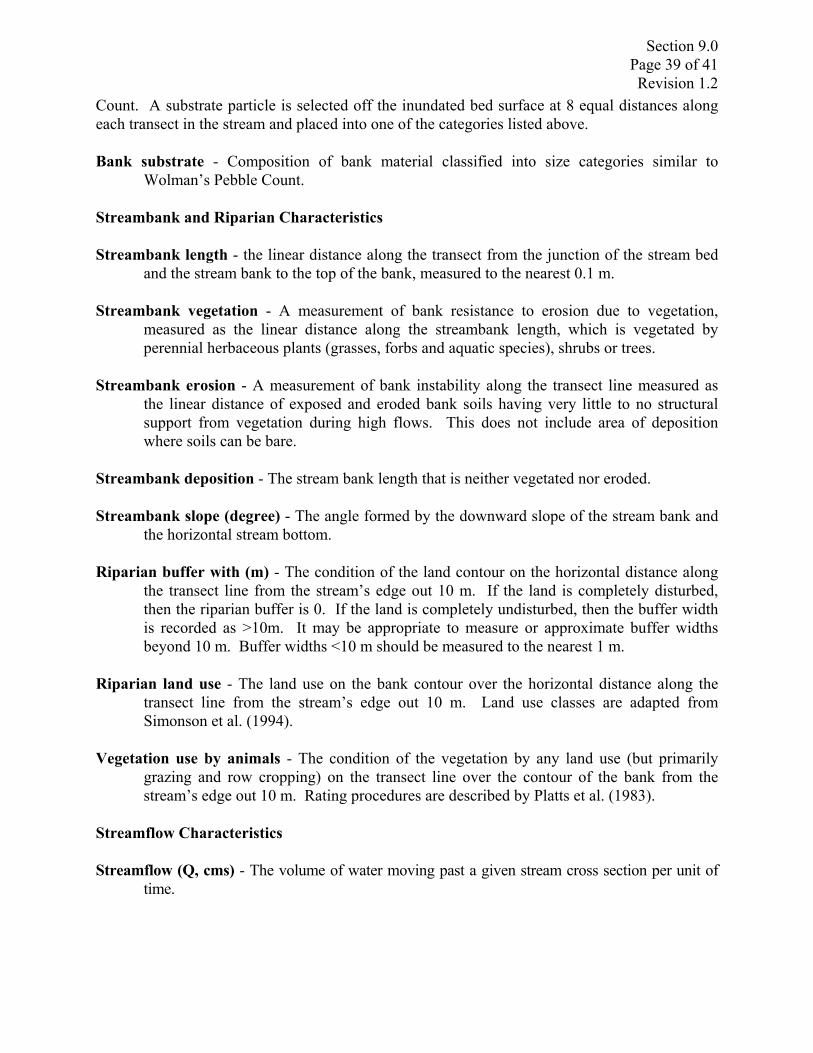
Section 9.0 Page 39 of 41 Revision 1.2
Count. A substrate particle is selected off the inundated bed surface at 8 equal distances along each transect in the stream and placed into one of the categories listed above. Bank substrate - Composition of bank material classified into size categories similar to
Wolman’s Pebble Count.
Streambank and Riparian Characteristics
Streambank length - the linear distance along the transect from the junction of the stream bed and the stream bank to the top of the bank, measured to the nearest 0.1 m.
Streambank vegetation - A measurement of bank resistance to erosion due to vegetation,
measured as the linear distance along the streambank length, which is vegetated by perennial herbaceous plants (grasses, forbs and aquatic species), shrubs or trees.
Streambank erosion - A measurement of bank instability along the transect line measured as
the linear distance of exposed and eroded bank soils having very little to no structural support from vegetation during high flows. This does not include area of deposition where soils can be bare.
Streambank deposition - The stream bank length that is neither vegetated nor eroded. Streambank slope (degree) - The angle formed by the downward slope of the stream bank and
the horizontal stream bottom. Riparian buffer with (m) - The condition of the land contour on the horizontal distance along
the transect line from the stream’s edge out 10 m. If the land is completely disturbed, then the riparian buffer is 0. If the land is completely undisturbed, then the buffer width is recorded as >10m. It may be appropriate to measure or approximate buffer widths beyond 10 m. Buffer widths <10 m should be measured to the nearest 1 m.
Riparian land use - The land use on the bank contour over the horizontal distance along the
transect line from the stream’s edge out 10 m. Land use classes are adapted from Simonson et al. (1994).
Vegetation use by animals - The condition of the vegetation by any land use (but primarily
grazing and row cropping) on the transect line over the contour of the bank from the stream’s edge out 10 m. Rating procedures are described by Platts et al. (1983).
Streamflow Characteristics Streamflow (Q, cms) - The volume of water moving past a given stream cross section per unit of
time.

Section 9.0 Page 40 of 41 Revision 1.2
Physical Fish Cover Overhanging vegetation - If present, the bankside, banktop, and non-inundated vegetation that
currently overhangs the water surface. Measured as the horizontal distance along the transect line from the water’s edge to the furthest point over the water surface that the vegetation protrudes, to the nearest 0.1 m.
Undercut bank - If present, the horizontal distance along the transect line from the furthest
point of bank protrusion and the furthest undercut of the bank, to the nearest 0.1 m. Instream vegetation - If present the inundated macrophytic vegetation (submergent or
emergent) within the stream channel. Measured as the total horizontal distance along the transect that has instream vegetation present as described, to the nearest 0.1 m.
Large woody debris (LWD), occurrence of - Generally, LWD are pieces of wood that are
minimally 10 cm in diameter and 3 m long that occur within the bankfull channel providing potential cover for organisms. Measured along the transect and within one mean stream width separately as the number of pieces within the stream’s different zones.
Large woody debris (LWD), volume and orientation - Volume (cubic meters) of those same
pieces within four zones calculated by measuring length and diameter of each piece of LWD. Orientation is recorded as the degrees to which the woody debris is predominately orientated with respect to the channel. Woody debris orientated completely upstream (i.e., root wad on downstream end) would be recorded as 180 while that orientated perpendicular to the channel would be recorded as 90, and that orientated completely downstream (i.e., root wad on upstream end) would be recorded as 0. See Robison and Beshta (1990).

Section 10.0 Page 1 of 2 Revision 1.2
10.0. REFERENCE CITED Ball, J. 1982. Stream Classification Guidelines for Wisconsin. Wisconsin Dept. Nat. Res. Tech.
Bull., Wisconsin Dept. Nat. Res., Madison, WI. Bisson, P.A., J.L. Neilsen, R.A. Palmason, and L.E. Grove. 1982. A system of naming habitat
types in small streams, with examples of habitat utilizations by salmonids during low stream flow. Pp. 62-73 IN: N.B. Armantrout (ed.). Acquisition and Utilization of Aquatic Habitat Inventory Information. Symposium Proceedings, October 18-30, 1981, Portland, Oregon. The Hague Publsing, Billings, Montana.
Courtemanch, D.L. 1984. A Closing Artificial Substrate Device for Sampling Benthic
Macroinvertebrates in Deep Rivers. Freshwater Invertebrate Biology Vol. 3(3). Pp 143-146. Frissell, C.A., W.J. Liss, C. E. Warren, ad M.D Hurley. 1986. A hierarchical
framework for stream habitat classification: viewing streams in a watershed context. Environmental Management 10:199-214.
Gordon, N.D., T.A. McMahon, and B.L. Finlayson. 1992. Stream hydrology: an introduction for
ecologists. John Wilery and Sons. New York, New York. Harrelson, C.C., C.L. Rawlinds, and J.P. Potyondy. 1994. Stream channel reference sites: an illustrated
guide to field technique. General Technical Report RM-245. Fort Collins, CO: U.S. Department of Agriculture, Forest Service, Rocky Mountain Forest and Range Experiment Station. 61 p.
Hayslip, G.A. 1992. EPA Region 10 In-Stream Biological Monitoring Handbook (Draft). EPA
Region 10, Env. Serv. Div., Seattle, Wa. Jessen, R. and R. Lound. 1962. An Evaluation of a Survey Technique for Submerged Aquatic
Plants. Minnesota Dept. of Conservation, Division of Game and Fish, Game Investigational Report No. 6.
Kaufmann, P.R. and E.G. Robison. 1998. Physical Habitat Assessment. pp 77-118 In: Lazorchak,
J.L., Klemm, D.J., and D.V. Peck (editors)., Environmental Monitoring and Assessment Program – Surface Waters: Field Operations and Methods for Measuring the Ecological Condition of Wadeable Streams. EPA/620/R-94/004F. U.S. Environmental Protection Agency, Washington, D.C.
King, K.W. 1993. A Bioassessment Method for use in Wyoming Stream and River Water Quality
Monitoring. Wyoming Department of Environmental Quality. 84pp.

Section 10.0 Page 2 of 2 Revision 1.2
Lemmon, P.E. 1957. A new instrument for measuring forest overstory density. Journal of Forestry 55(9):667-669.
Leopold, L.B. 1994. A View of the River. Harvard University Press, Cambridge, MA. 298 pp. Milewski, C.L. 2001. Local and Systemic Controls on Fish and Fish Habitat in South Dakota
Rivers and Streams: Implications for Management. Ph.D. Dissertation, South Dakota State University, Brookings, South Dakota. 177 pp.
Milewski, C.L. 2002. Personal Communication. Minn. DNR. 1993. Manual of Instructions for Lake Survey. Special publication No. 147 pp 3-4 - Mulvey, M., L. Caton, and R. Hafele. 1992. Oregon Nonpoint Source Monitoring Protocols
Stream Bioassessment Field Manual for Macroinvertebrates and Habitat Assessment. Oregon Department of Environmental Quality, Laboratory Biomonitoring Section. 1712 S.W. 11th Ave. Portland, Oregon, 97201. 40 p.
Nickum, J.G. 1969. Limnological Survey of Lake Tetonkaha and Adjacent Marsh. Unpublished
report. Department of Fish and Wildlife, SDSU, Brookings, South Dakota. Newbury, R.W., and M.N. Gaboury. 1993. Stream analysis and fish habitat design: a field manual.
Newbury Hydraulics Ltd. and the Manitoba Habitat Heritage Corporation. Peck, D.V., J.M. Lazorchak, and D.J. Klemm (editors). Unpublished draft 2001. Environmental
Monitoring and Assessment Program – Surface Waters: Western Pilot Study Field Operations Manual for Wadeable Streams. EPA/XXX/X-XX/XXXX. U.S. Environmental Protection Agency, Washington, D.C.
Plafkin, J.L., M.T. Barbour, K.D. Porter, S.K. Gross, and R.M. Hughes. 1989. Rapid
Bioassessment Protocols for use in Streams and Rivers. Office of Water (Wh-553), EPA/444/4-89-001. Washington, D.C.
Platts, W.S., W.F. Megahan, and G.W. Minshall. 1983. Methods for Evaluating Stream, Riparian,
and Biotic Conditions. General Tech. Rpt. INT-138. U.S. Dept. Agric., Forest Serv., Ogden, UT. 71 p

Section 10.0 Page 3 of 2 Revision 1.2
Platts, W.S., C. Armour, G.D. Booth, M., Bryant, J.L. Bufford, P. Cuplin, S. Jensen, G.W.
Lienkaemper, G.W. Minshall, S.B. Monson, R.L. Nelson, J.R.Sedell, J.S. Tuhy. 1987. Methods for evaluating riparian habitats with applications to management. Gen. Tech. Rpt. INT-221. USDA Forest Service, Ogden UT.
Robison, E.G., and R.L. Beschta. 1990. Characteristics of coarse woody debris for several coastal
stream of southeast Alaska, USA. Canadian Journal of Fisheries and Aquatic Sciences 47:1684-1693.
Rosgen, D. 1994. A classification of natural rivers. Catena 22:169-199. Rosgen, D. 1996. Applied River Morphology. Wildland Hydrology. Pagosa Springs, Co. Rothrock, E.P. 1943. A Geology of South Dakota I. The Surface. State Geological Survey Bulletin
13. 88 pp. Simonson, T.D., J. Lyons, and P.D Kanehl. 1994. Quantifying fish habitat in streams: transect spacing,
sample size, and a proposed framework. 14:607-615. State of Vermont. 1990. Indirect Discharge Rules. Agency of Natural Resources Department of
Environmental Conservation. 244 pp. Steffen, L. 2001. Fluvial Geomorphology Workshop. Spearfish, SD,. May 2001. Wind River Clean Lakes Program Quality Assurance Plan. 1990. Wind River Environmental Quality
Commission, Shoshone and Northern Arapaho Tribes, Ft. Washakie, Wyoming. 19 pp. U.S. Environmental Protection Agency. 1990. Macroinvertebrate Field and Laboratory Methods
for Evaluating the Biological Integrity of Surface Waters. 600/4-90/030. Office of Research and Development, Washington, D.C. 256 pp.
US EPA. 1991. Volunteer Lake Monitoring: A Methods Manual. EPA 440/4-91-002. Office of
Water. Washington, DC Wolman, M.G. 1954. A method of sampling coarse river-bed material. Transactions of the
American Geophysical Union 35:951-956.

Appendix A
LAKE HABITAT ASSESSMENT FIELD DATA SHEET— MACROPHYTE SURVEY

SD WRAP LAKE HABITAT ASSESSMENT FIELD DATA SHEET—MACROPHYTE SURVEY
LAKE NAME
DATE /TIME
STATION #____________________
TRANSECT #
INVESTIGATORS
Condition CategoryHabitat
Parameter Optimal Suboptimal Marginal Poor
1. Bank Stability
Banks stable; evidence of erosion or bank failure absent or minimal; little potential for future problems. <5% of bank affected.
Moderately stable; infrequent, small areas of erosion mostly healed over. 5-30% of bank in reach has areas of erosion.
Moderately unstable; 30-60% of bank in reach has areas of erosion; high erosion potential during floods.
Unstable; many eroded areas; "raw" areas frequent along straight sections and bends; obvious bank sloughing; 60-100% of bank has erosional scars.
SCORE ___ 10 9 8 7 6 5 4 3 2 1 0
2. Vegetative Protection
More than 90% of the bank surfaces and immediate riparian zone covered by native vegetation, including trees, understory shrubs, or nonwoody macrophytes; vegetative disruption through grazing or mowing minimal or not evident; almost all plants allowed to grow naturally.
70-90% of the bank surfaces covered by native vegetation, but one class of plants is not well-represented; disruption evident but not affecting full plant growth potential to any great extent; more than one-half of the potential plant stubble height remaining.
50-70% of the bank surfaces covered by vegetation; disruption obvious; patches of bare soil or closely cropped vegetation common; less than one-half of the potential plant stubble height remaining.
Less than 50% of the bank surfaces covered by vegetation; disruption of bank vegetation is very high; vegetation has been removed to 5 centimeters or less in average stubble height.
SCORE ___ 10 9 8 7 6 5 4 3 2 1 0
3. Riparian Vegetative Zone Width
Width of riparian zone >18 meters; human activities (i.e., parking lots, roadbeds, clear-cuts, lawns, or crops) have not impacted zone.
Width of riparian zone 12-18 meters; human activities have impacted zone only minimally.
Width of riparian zone 6-12 meters; human activities have impacted zone a great deal.
Width of riparian zone <6 meters: little or no riparian vegetation due to human activities.
SCORE 10 9 8 7 6 5 4 3 2 1 0
Total Score __________ Maximum Depth of Plant Colonization________ Density Rating Chart
Rake Recovery of Aquatic Plant Type
Density Descriptive Term Rake Recovery of Aquatic Plant Type
Density Descriptive Term
Taken in all 4 casts (teeth of rake full) 5 Dense Taken in 2 casts 2 Scattered Taken in 4 casts 4 Heavy Taken in 1 cast 1 Sparse Taken in 3 casts 3 Moderate
Location A Secchi Location B Secchi
Lake Depth Position (% recovery) Lake Depth Position (% recovery)
Species 12 3 6 9 Density Species 12 3 6 9 Density
Location C Secchi Location D Secchi
Lake Depth Position (% recovery) Lake Depth Position (% recovery)
Species 12 3 6 9 Density Species 12 3 6 9 Density

Appendix B
SD WRAP IN-LAKE SAMPLING FIELD DATA COLLECTION SHEET

South Dakota WRAP In-lake Sampling Field Data Collection Sheet
Lake Name ________________________ Lake ID ___________________ Sampler(s) _________________________ Air Temp. _________________°C Date __________________ Conductivity _______________ Time __________________ Precip. N Mi Mo E S Turbidity:_____ (NTU) GPS Unit __________________________ Wind: N Mi Mo E S Film: N Mi Mo E S Latitude ___________________________ Odor: N Mi Mo E S Color __________ Longitude _________________________ Dead Fish: N Mi Mo E S Ice Cover ____ m
Site _______________ Aperture Size ________(m)
Site _______________ Aperture Size ________(m)
Site _______________ Aperture Size __________(m)
Tow Length _________(m) Tow Length __________(m) Tow Length __________(m) Counter Start ____________ Counter Start ______________ Counter Start _______________ Counter Stop ____________ Counter Stop ______________ Counter Stop _______________ Depth Temp. DO Depth Temp. DO Depth Temp. DO
_____ _____ _____ _____ _____ _____ _____ _____ _____ _____ _____ _____ _____ _____ _____ _____ _____ _____ _____ _____ _____ _____ _____ _____ _____ _____ _____ _____ _____ _____ _____ _____ _____ _____ _____ _____ _____ _____ _____ _____ _____ _____ _____ _____ _____ _____ _____ _____ _____ _____ _____ _____ _____ _____ _____ _____ _____ _____ _____ _____ _____ _____ _____ _____ _____ _____ _____ _____ _____ _____ _____ _____ _____ _____ _____ _____ _____ _____ _____ _____ _____ _____ _____ _____ _____ _____ _____ _____ _____ _____ _____ _____ _____ _____ _____ _____ _____ _____ _____ _____ _____ _____ _____ _____ _____ _____ _____ _____ _____ _____ _____ _____ _____ _____ _____ _____ _____ **** Record depth in meters and temperature in Celsius Total Depth ____________ Total Depth _____________ Total Depth _____________ Secchi Depth _____, _____ Secchi Depth ______, _____ Secchi Depth ______, ______ Surface pH _____________ Surface pH _____________ Surface pH ______________ Bottom pH ______________ Bottom pH _____________ Bottom pH ______________ Surface Turbid __________ Surface Turbid ____________ Surface Turbid ____________ Bottom Turbid ___________ Bottom Turbid ____________ Bottom Turbid ____________ Surface Conduct _________ Surface Conduct ___________ Surface Conduct ___________ Bottom Conduct _________ Bottom Conduct ___________ Bottom Conduct ___________
Total Tow Length (for composite zooplankton samples) ___________________________ (m) Average Depth __________________(m) Average Secchi Depth ____________ (m)
Average Surface pH ______________ Average Bottom pH ______________ Average Surface Conductivity ___________ Average Bottom Conductivity _________ Average Surface Turbidity _________ Average Bottom Turbidity _____________ Notes:

South Dakota WRAP In-lake Zooplankton Sampling Field Data Collection Sheet
Lake Name ________________________ Lake ID ___________________ Sampler(s) _________________________ Air Temp. _________________°C Date __________________ Conductivity _______________ Time __________________ Precip. N Mi Mo E S Turbidity:_____ (NTU) GPS Unit __________________________ Wind: N Mi Mo E S Film: N Mi Mo E S Latitude ___________________________ Odor: N Mi Mo E S Color __________ Longitude _________________________ Dead Fish: N Mi Mo E S Ice Cover ____ m Type of Sampling Device (Circle one)
Wisconsin Net Student Net 0.5 or 1.0 meter Plankton Net
Site _______________ Aperture Size ________(m) Mesh Size __________(µm)
Site _______________ Aperture Size __________(m) Mesh Size ____________(µm)
Site _______________ Aperture Size _____________(m) Mesh Size ______________(µm)
Tow Length _________(m) Tow Length __________(m) Tow Length __________(m) Beginning Tow Counter Start ____________ Counter Start ______________ Counter Start _______________ Counter Stop ____________ Counter Stop ______________ Counter Stop _______________ Ending Tow Counter Start ____________ Counter Start ______________ Counter Start _______________ Counter Stop ____________ Counter Stop ______________ Counter Stop _______________
Total Depth ____________ Total Depth _____________ Total Depth _____________ Secchi Depth _____, _____ Secchi Depth ______, _____ Secchi Depth ______, ______
Total Tow Length (for composite zooplankton samples) ___________________________ (m) Average Depth __________________(m) Average Secchi Depth ____________ (m)
Observations:

Appendix C
SOUTH DAKOTA WATER QUALITY DATA SHEETS


Appendix D
PERIPHYTON SAMPLING DATA SHEETS

Periphyton Map, Measurements and Documentation
Project Site ID: Stream Name: Date:
Draw a map of the site with location of most upstream and most downstream transects. Include locations of photographic points, direction of photograph, and frame number.
Approximate Distance

Appendix E
MACROINVERTEBRATE SAMPLER CONSTRUCTION AND SAMPLING DATA SHEETS
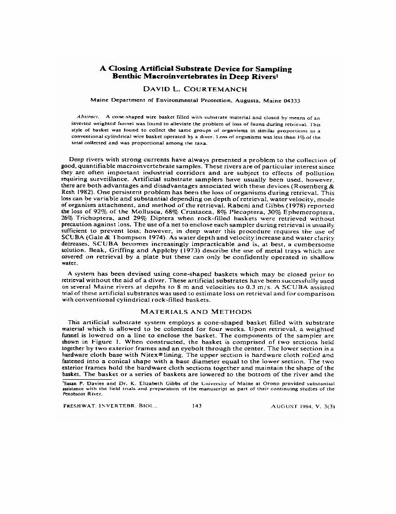
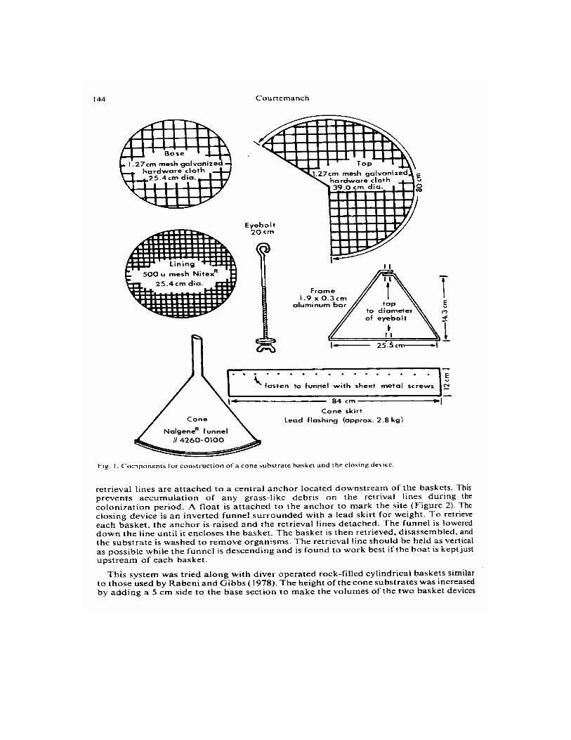


Modified Artificial Substrate Sampler The following is a model for constructing a modified sampler (modified from Vermont DEC 1990). Sampler is constructed of 1.27 cm mesh galvanized hardware cloth. Assemble sampler using cable ties. This design is used in shallow riffle habitat
5 cm 5 cm
20 cm
5 cm
20 cm
30 cm

Macroinvertebrate Field Data Sheet
Project Site ID: Stream Name: Date:
Draw a map of the site with location of most upstream and most downstream transects. Include locations of photographic points, direction of photograph, and frame number.
Approximate Distance

APPENDIX F
HABITAT FIELD COLLECTION DATASHEETS
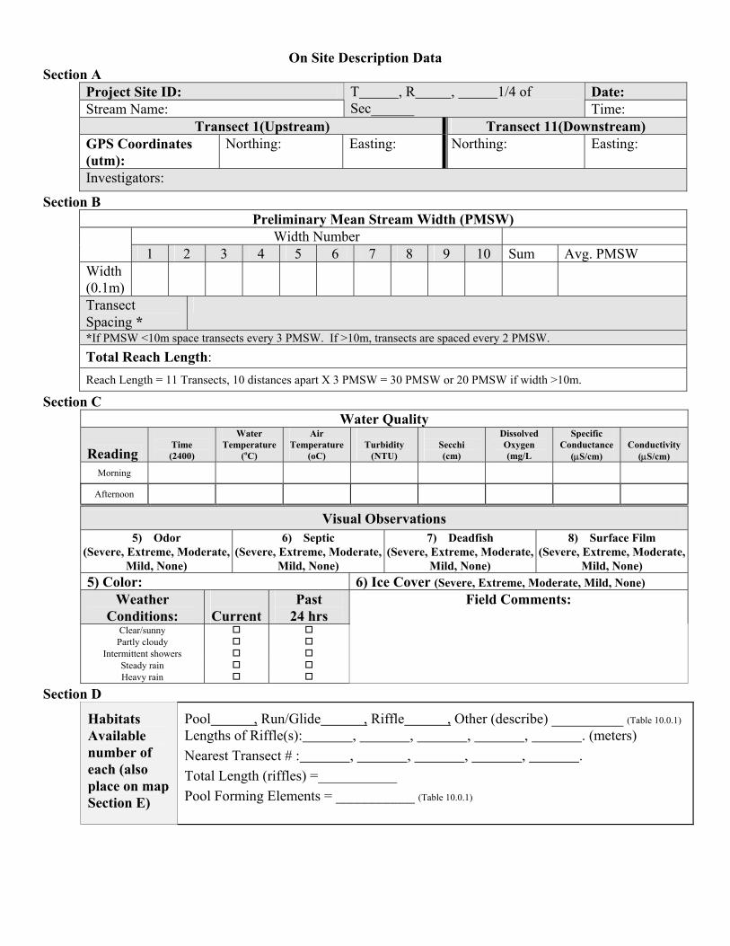
On Site Description Data Section A
Project Site ID: Date: Stream Name:
T , R , 1/4 of Sec______ Time:
Transect 1(Upstream) Transect 11(Downstream) GPS Coordinates (utm):
Northing: Easting: Northing: Easting:
Investigators:
Section B Preliminary Mean Stream Width (PMSW)
Width Number 1 2 3 4 5 6 7 8 9 10 Sum Avg. PMSW
Width (0.1m)
Transect Spacing *
*If PMSW <10m space transects every 3 PMSW. If >10m, transects are spaced every 2 PMSW.
Total Reach Length: Reach Length = 11 Transects, 10 distances apart X 3 PMSW = 30 PMSW or 20 PMSW if width >10m.
Section C Water Quality
Reading
Time (2400)
Water Temperature
(oC)
Air Temperature
(oC)
Turbidity
(NTU)
Secchi (cm)
Dissolved Oxygen (mg/L
Specific Conductance
(µS/cm)
Conductivity
(µS/cm)
Morning Afternoon
Visual Observations 5) Odor
(Severe, Extreme, Moderate, Mild, None)
6) Septic (Severe, Extreme, Moderate,
Mild, None)
7) Deadfish (Severe, Extreme, Moderate,
Mild, None)
8) Surface Film (Severe, Extreme, Moderate,
Mild, None) 5) Color: 6) Ice Cover (Severe, Extreme, Moderate, Mild, None)
Weather Conditions:
Current
Past 24 hrs
Field Comments:
Clear/sunny Partly cloudy
Intermittent showers Steady rain Heavy rain
Section D Habitats Available number of each (also place on map Section E)
Pool , Run/Glide , Riffle , Other (describe) __________ (Table 10.0.1)
Lengths of Riffle(s): , , , , . (meters) Nearest Transect # : , , , , . Total Length (riffles) =___________ Pool Forming Elements = ___________ (Table 10.0.1)
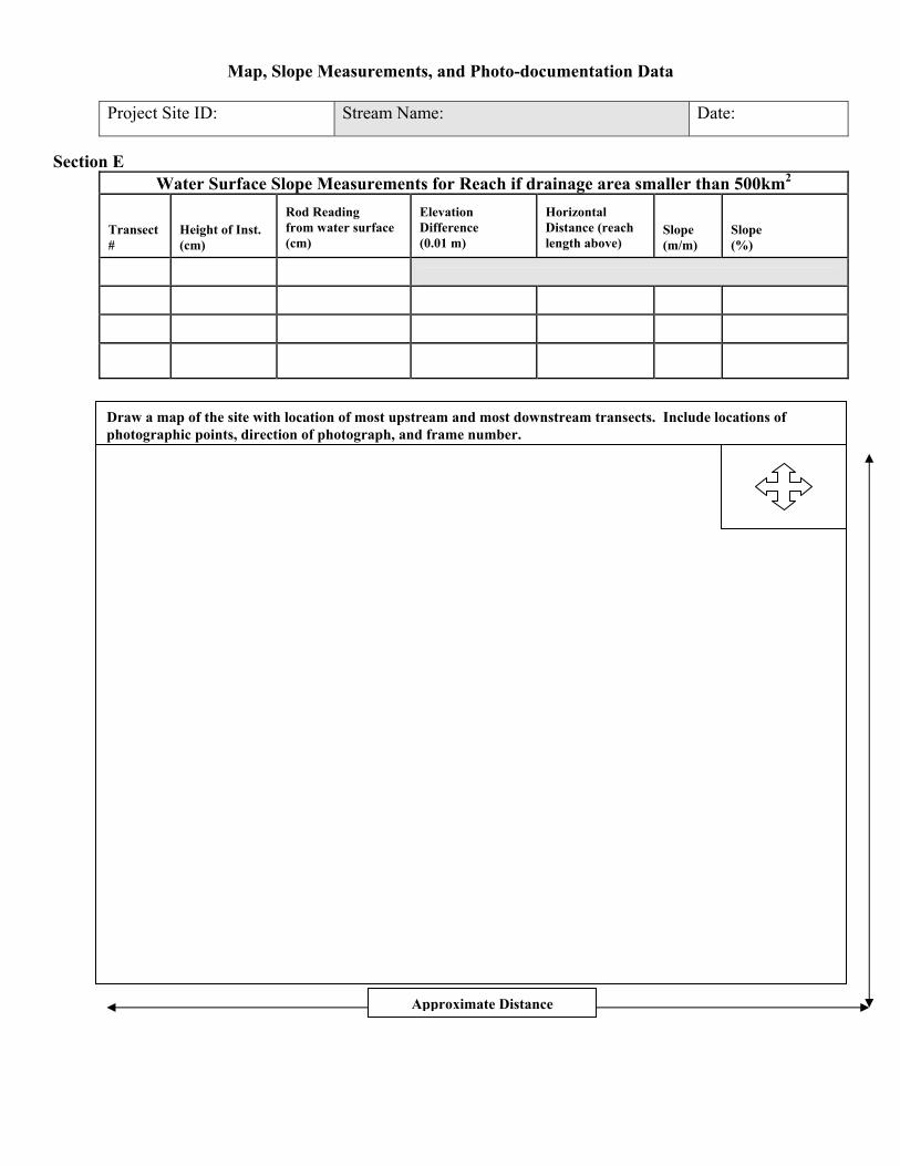
Map, Slope Measurements, and Photo-documentation Data Project Site ID: Stream Name: Date:
Section E Water Surface Slope Measurements for Reach if drainage area smaller than 500km2
Transect #
Height of Inst. (cm)
Rod Reading from water surface (cm)
Elevation Difference (0.01 m)
Horizontal Distance (reach length above)
Slope (m/m)
Slope (%)
Draw a map of the site with location of most upstream and most downstream transects. Include locations of photographic points, direction of photograph, and frame number.
Approximate Distance
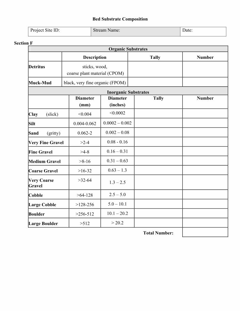
Bed Substrate Composition Project Site ID: Stream Name: Date:
Section F Organic Substrates
Description
Tally
Number
Detritus
sticks, wood,
coarse plant material (CPOM)
Muck-Mud
black, very fine organic (FPOM)
Inorganic Substrates
Diameter (mm)
Diameter (inches)
Tally Number
Clay (slick)
<0.004 <0.0002
Silt
0.004-0.062 0.0002 – 0.002
Sand (gritty)
0.062-2 0.002 – 0.08
Very Fine Gravel
>2-4 0.08 - 0.16
Fine Gravel
>4-8 0.16 – 0.31
Medium Gravel
>8-16 0.31 – 0.63
Coarse Gravel
>16-32 0.63 – 1.3
Very Coarse Gravel
>32-64 1.3 – 2.5
Cobble
>64-128 2.5 – 5.0
Large Cobble
>128-256 5.0 – 10.1
Boulder
>256-512 10.1 – 20.2
Large Boulder
>512 > 20.2
Total Number:

Section G
Large Woody Debris Data Project Site ID:_________________Stream Name:____________Date:_________Page____of____
Transect Spacing
Log Jam Number
LWD
Number
Zone
Meander Location
Habitat
Association
Angle
Length
Diameter
Zone: Zone 1 is water surface at baseflow, Zone 2 is between baseflow surface and bankfull flow surface, Zone 3 is bankfull channel width above bankfull flow surface. Meander Location: IM=inside meander, OM=outside meander, CO=crossover, SS=straight section Habitat Association: PL=pool, RF=riffle, RN=run
LARGE WOODY DEBRIS CATEGORIES (≥10 cm small end diameter; ≥1.5 m length) Categories 1 2 3 4 Diameter Large End 0.1-<0.3m 0.3-0.6m 0.6-0.8m >0.8m Length >1.5-5m 5-15m >15m -

Stream Shade and Canopy Cover Monitoring
Project Site ID: Stream Name: Date:
Section H
Site Name:
Date:
Reach Length:
Transect Interval: Initials:
Transect Left Bank
Right Bank
Center Upstream
Center Right
Center Downstream
Center Left
1
2
3
4
5
6
7
8
9
10
11
Total Total by
bank (Out of 187)
Total of Center Positions
(Out of 748)
Percent Cover
(by Bank)
Percent Cover
(for Reach)
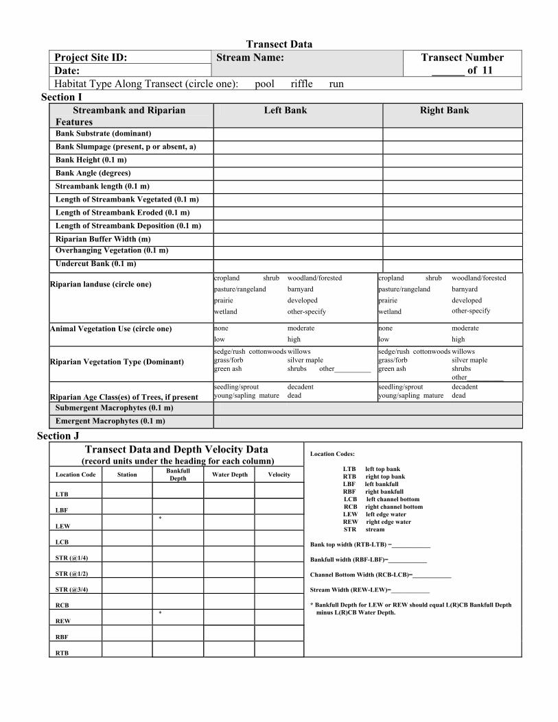
Transect Data Project Site ID: Date:
Stream Name: Transect Number ______ of 11
Habitat Type Along Transect (circle one): pool riffle run Section I
Streambank and Riparian Features
Left Bank Right Bank
Bank Substrate (dominant) Bank Slumpage (present, p or absent, a) Bank Height (0.1 m) Bank Angle (degrees) Streambank length (0.1 m) Length of Streambank Vegetated (0.1 m) Length of Streambank Eroded (0.1 m) Length of Streambank Deposition (0.1 m) Riparian Buffer Width (m) Overhanging Vegetation (0.1 m) Undercut Bank (0.1 m)
Riparian landuse (circle one)
cropland shrub pasture/rangeland prairie wetland
woodland/forested barnyard developed other-specify
cropland shrub pasture/rangeland prairie wetland
woodland/forested barnyard developed other-specify
Animal Vegetation Use (circle one) none low
moderate high
none low
moderate high
Riparian Vegetation Type (Dominant)
sedge/rush cottonwoodsgrass/forb green ash
willows silver maple shrubs other__________
sedge/rush cottonwoodsgrass/forb green ash
willows silver maple shrubs other__________
Riparian Age Class(es) of Trees, if present
seedling/sprout young/sapling mature
decadent dead
seedling/sprout young/sapling mature
decadent dead
Submergent Macrophytes (0.1 m)
Emergent Macrophytes (0.1 m)
Section J Transect Data and Depth Velocity Data
(record units under the heading for each column) Location Code Station Bankfull
Depth Water Depth Velocity
LTB
LBF
LEW
*
LCB
STR (@1/4)
STR (@1/2)
STR (@3/4)
RCB
REW
*
RBF
RTB
Location Codes:
LTB left top bank RTB right top bank LBF left bankfull RBF right bankfull LCB left channel bottom RCB right channel bottom LEW left edge water REW right edge water STR stream
Bank top width (RTB-LTB) =____________ Bankfull width (RBF-LBF)=____________ Channel Bottom Width (RCB-LCB)=____________ Stream Width (REW-LEW)=____________ * Bankfull Depth for LEW or REW should equal L(R)CB Bankfull Depth
minus L(R)CB Water Depth.
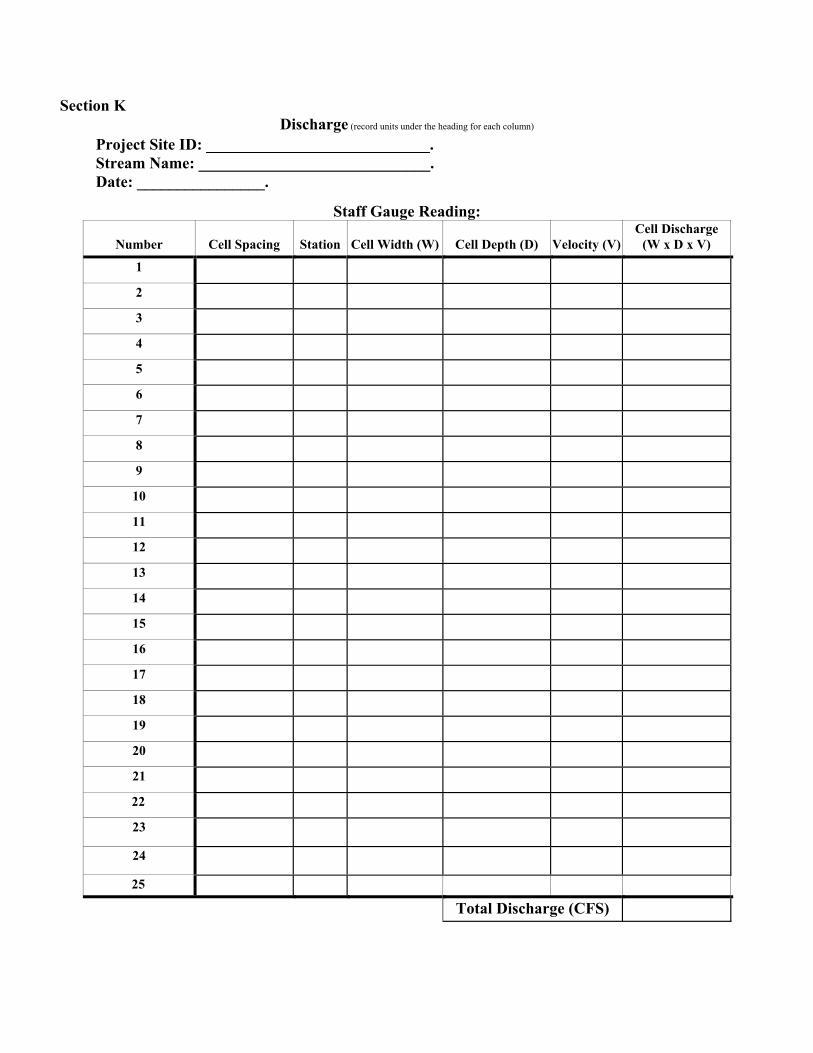
Section K Discharge (record units under the heading for each column)
Project Site ID: ____________________________. Stream Name: _____________________________. Date: ________________.
Staff Gauge Reading:
Number
Cell Spacing
Station
Cell Width (W)
Cell Depth (D)
Velocity (V) Cell Discharge
(W x D x V)
1
2
3
4
5
6
7
8
9
10
11
12
13
14
15
16
17
18
19
20
21
22
23
24
25
Total Discharge (CFS)

75 copies of this document were printed by the Department of Environment and Natural Resources at a cost of $4.20 per copy.