NIST Special Publication 260-173

Standard Reference Materials:

SRM 1450d, Fibrous-Glass Board, for Thermal Conductivity from 280 K to 340 K

Robert R. Zarr Amanda C. Harris

John F. Roller Stefan D. Leigh

NIST Special Publication 260-173

Standard Reference Materials:

SRM 1450d, Fibrous-Glass Board, for Thermal Conductivity from 280 K to 340 K

Robert R. Zarr

Amanda C. Harris John F. Roller

Engineering Laboratory Building Environment Division

Stefan D. Leigh Information Technology Laboratory

Statistical Engineering Division

National Institute of Standards and Technology Gaithersburg, MD 20899-8632

August 2011

U.S. Department of Commerce Rebecca M. Blank, Acting Secretary

National Institute of Standards and Technology

Patrick D. Gallagher, Under Secretary of Commerce for Standards and Technology and Director

Certain commercial entities, equipment, or materials may be identified in this

document in order to describe an experimental procedure or concept adequately. Such identification is not intended to imply recommendation or endorsement by the National Institute of Standards and Technology, nor is it intended to imply that the entities, materials, or equipment are necessarily the best available for the purpose.

National Institute of Standards and Technology Special Publication 260-173 Natl. Inst. Stand. Technol. Spec. Publ. 260-173, 128 pages (August 2011)

CODEN: NSPUE2

iii

Abstract Thermal conductivity measurements at and near room temperature are presented as the ba-sis for certified values of thermal conductivity for SRM 1450d, Fibrous Glass Board. The measurements have been conducted in accordance with a randomized full factorial experi-mental design with two variables, bulk density and temperature, using the NIST 1016 mm line-heat-source guarded-hot-plate apparatus. The thermal conductivity of the SRM speci-mens was measured over a range of bulk densities from 114 kg·m-3 to 124 kg·m-3 and mean temperatures from 280 K to 340 K. Uncertainties of the measurements, consistent in for-mat with current international guidelines, have been prepared. Statistical analyses of the physical properties from the SRM are presented and include variations between boards, as well as within board.

Each unit of SRM 1450d is individually certified for bulk density, ρ, and batch certified for thermal conductivity with the following equation:

( )4λ 1.10489 10 mT−= × ×

where λ is the predicted thermal conductivity (W·m-1·K-1) and Tm is the mean temperature (K) valid over the temperature range of 280 K to 340 K. The expanded uncertainty for λ values from the above equation is 1 % with a coverage factor of approximately k = 2.

Keywords calibration; bulk density; fibrous glass board; guarded-hot-plate apparatus; heat-flow-meter apparatus; standard reference material; SRM 1450d; thermal conductivity; thermal insulation; uncertainty

iv

TABLE OF CONTENTS

Nomenclature...................................................................................................................... 1 1 Introduction................................................................................................................. 4 2 Historical Background ................................................................................................ 6

2.1 Early Program and Establishment of SRMs 1450 and 1450a............................. 6 2.2 SRM 1450b ......................................................................................................... 6 2.3 SRM 1450c ......................................................................................................... 7 2.4 SRM 1450d ......................................................................................................... 7

3 Terms and Definitions................................................................................................. 8

3.1 Reference Materials Definitions ......................................................................... 8 3.2 Thermal Insulation Definitions ........................................................................... 9 3.3 Uncertainty Definitions..................................................................................... 10

4 Certification Project Design...................................................................................... 12

4.1 Project Definition and Scope for Intended Use ................................................ 12 4.2 Material ............................................................................................................. 12

4.2.1 Requirements ............................................................................................ 12 4.2.2 Fabrication ................................................................................................ 13 4.2.3 Fabrication Controls.................................................................................. 13 4.2.4 Auxiliary Material Fabrication ................................................................. 14

4.3 Preparation ........................................................................................................ 14 4.3.1 Inspection and Storage.............................................................................. 14 4.3.2 General Sampling Procedure .................................................................... 14

4.4 Measurement Methods...................................................................................... 15 4.4.1 Bulk Density Study................................................................................... 15 4.4.2 Thermal Conductivity Measurements....................................................... 15

5 Measurement Uncertainty......................................................................................... 16

5.1 Combined Standard Uncertainty....................................................................... 16 5.2 Expanded Uncertainty....................................................................................... 16 5.3 Type A and Type B Uncertainty Evaluations ................................................... 17 5.4 Degrees of Freedom.......................................................................................... 17 5.5 Comments on Approach ................................................................................... 17

6 Bulk Density Study................................................................................................... 18

6.1 Panel Mass Measurements................................................................................ 18 6.2 Dimensional Measurements.............................................................................. 18

6.2.1 Lateral Panel Dimensions – Length and Width ........................................ 19 6.2.2 Thickness .................................................................................................. 21

6.3 Homogeneity Assessment................................................................................. 22 6.3.1 Tabulated Results...................................................................................... 22 6.3.2 Graphical Analyses ................................................................................... 31

v

6.3.3 Summary Statistics.................................................................................... 38 6.3.4 Between- and Within-Panel Thickness Variations ................................... 38 6.3.5 Between-Panel Bulk Density Variations .................................................. 40 6.3.6 Anomalous Panels (Outliers) .................................................................... 41

6.4 Establishing and Demonstrating Traceability................................................... 41 6.4.1 Mass .......................................................................................................... 41 6.4.2 Length Dimensions ................................................................................... 41

6.5 Bulk Density Uncertainty ................................................................................. 41 7 Thermal Conductivity Measurements....................................................................... 43

7.1 Experimental Design and Initial Model............................................................ 43 7.1.1 Model Input Quantities – Bulk Density (ρ) and Temperature (T) ............ 43 7.1.2 Other Quantities ........................................................................................ 43

7.2 Guarded-Hot-Plate Guard Insulation ................................................................ 44 7.3 Specimen Selection........................................................................................... 45 7.4 Thermal Conductivity Apparatus...................................................................... 45

7.4.1 Guarded-Hot-Plate Method....................................................................... 45 7.4.2 1016 mm Guarded-Hot-Plate Apparatus .................................................. 47

7.5 Establishing and Demonstrating Traceability................................................... 47 7.5.1 Specimen Heat Flow - Q........................................................................... 48 7.5.2 Temperature Difference - ΔT .................................................................... 49 7.5.3 Specimen Thickness - L ............................................................................ 49 7.5.4 Meter Area - A .......................................................................................... 50 7.5.5 Influence (Secondary) Quantities ............................................................. 50

7.6 Identification of Uncertainty Sources ............................................................... 51 8 Data and Uncertainty Evaluation .............................................................................. 53

8.1 Experimental Design Modification................................................................... 53 8.2 Guarded-Hot-Plate Data.................................................................................... 54

8.2.1 Data Acquisition ....................................................................................... 54 8.2.2 Data Summary (Tabular Format).............................................................. 54 8.2.3 Data Screening (Graphical Analysis)........................................................ 56 8.2.4 Data Evaluation – Characterization .......................................................... 56

8.3 Final Model....................................................................................................... 58 8.4 Uncertainty in Experimental Thermal Conductivity (λexp) ............................... 58

8.4.1 Uncertainty Budget ................................................................................... 59 8.4.2 Confidence Limits (Working-Hotelling Bands) ....................................... 60 8.4.3 Comments on Uncertainty Approach........................................................ 61 8.4.4 Supplemental Thermal Conductivity Data................................................ 61

9 Certification .............................................................................................................. 62

9.1 Properties of Interest ......................................................................................... 62 9.2 Values and Uncertainties .................................................................................. 62 9.3 Statement of Metrological Traceability ............................................................ 62 9.4 Instructions for Use........................................................................................... 62

9.4.1 Storage ...................................................................................................... 62

vi

9.4.2 Preparation and Conditioning Before Measurement................................. 63 9.4.3 Thermal Conductivity Measurement ........................................................ 63 9.4.4 Guidelines and Precautions....................................................................... 63

10 Acknowledgements............................................................................................... 63 11 References............................................................................................................. 63 Annex 1 – Mass Plots ....................................................................................................... 66 Annex 2 – Thickness Plots................................................................................................ 84 Annex 3 – Bulk Density Uncertainty, Extensive Details................................................ 102 Annex 4 – Thermal Conductivity Uncertainty, Extensive Details ................................. 105 Annex 5 – Supplemental Thermal Conductivity Measurements .................................... 115

vii

LIST OF TABLES Table 1 Thermal resistance and thermal conductivity of glass, silica, and polystyrene .......5 Table 2 Chronology and certified property ranges of SRM 1450, Fibrous Glass Board......6 Table 3 Physical properties of SRM 1450d units (450 panels)......................................23-30 Table 4 Summary statistics for the SRM 1450d production run (450 panels)....................38 Table 5 Full factorial (3×3) experimental design ...............................................................43 Table 6 Physical properties of guarded-hot-plate guard insulation ....................................44 Table 7 Test specimens for (3×3) experimental design ......................................................45 Table 8 Calibration information for the NIST 1016 mm guarded-hot-plate apparatus ......47 Table 9 Uncertainty sources for the NIST 1016 mm guarded-hot-plate apparatus...............51 Table 10 Full factorial (3×5) experimental design ...............................................................53 Table 11 Additional test specimens for (3×5) experimental design .....................................53 Table 12 Required tolerance limits for acceptable steady-state test data .............................54 Table 13 Thermal conductivity data (sorted by Tm and ρs)............................................................55 Table 14 Summary statistics for fixed- and recorded-value quantities.................................56 Table 15 Summary of linear profiles for λexp versus ρs (Fig. 14a) .......................................58 Table 16 Summary of regression statistics for λexp versus Tm (Fig. 14b)..............................58 Table A3-1 Uncertainty budget for height gage measurements..............................................103 Table A4-1 Summary of standard uncertainty components for u (Qm).....................................106 Table A4-2 Nominal settings for imbalance study (Yates order) .............................................107 Table A4-3 Test results for imbalance study (Yates order)......................................................107 Table A4-4 Parameter estimates and standard deviations for b1 and b2 in Eq. (A4-4)..............108 Table A4-5 Estimates for uc (ΔQ) ............................................................................................108 Table A4-6 Combined standard uncertainty (k = 1) for uc (Q) .................................................109 Table A4-7 Standard uncertainty components (k = 1) for T .....................................................110 Table A4-8 Standard uncertainty components (k = 1) for L .....................................................113 Table A4-9 Standard uncertainty components (k = 1) for A.....................................................114 Table A4-10 Combined standard uncertainty (k = 1) for uc (A)..................................................114 Table A5-1 Thermal conductivity data for specimen pair 184-369 ........................................115

viii

LIST OF FIGURES

Figure 1 Mass regain for Panel ID 438 after removal of panel from oven. Initial mass (m0) of 1.1060 kg was determined by linear extrapolation to time zero. .......................................19

Figure 2 a) Side view shows 610 mm height gage and right-angle fixture with insulation panel clamped between the aluminum jig plate and aluminum sheet. b) Front view shows panel length measurements at locations l1, l2, l3, l4, l5, and l6 (fixture and height gage are not shown). For a particular group of 50 panels, one panel was measured at all locations and the other 49 panels were measured at locations l2 and l5. ..................................................20

Figure 3 a) Front view shows 305 mm height gage and insulation panel (with workpiece) on granite surface plate. b) Top view shows an insulation panel and 8 thickness measurement loca-tions (L1 – L8) each in the geometric center of a 200 mm by 200 mm sub-area of the insula-tion panel. For a particular group of 50 panels, one panel was measured at all 8 locations and the other 49 panels were measured, in an alternating sequence, at the corner locations (L1, L3, L5, L7) and at the mid-center locations (L2, L4, L6, L8). ..........................................21

Figure 4 Graphical analysis of panel mass (n = 450): (a) run sequence plot, (b) lag plot, (c) histo-gram, (d) normal probability plot (normality index). Summary statistics: mean = 1.1466 kg, standard deviation = 0.0250 kg, range = 0.1635 kg. ........................................32

Figure 5 Graphical analysis of panel length (n = 450): (a) run sequence plot, (b) lag plot, (c) histo-gram, (d) normal probability plot (normality index). Summary statistics: mean = 610.92 mm, standard deviation = 0.62 mm, range = 2.85 mm. .........................................33

Figure 6 Graphical analysis of panel width (n = 450): (a) run sequence plot, (b) lag plot, (c) histo-gram, (d) normal probability plot (normality index). Summary statistics: mean = 610.85 mm, standard deviation = 0.56 mm, range = 3.00 mm. .........................................34

Figure 7 Graphical analysis of panel area (n = 450): (a) run sequence plot, (b) lag plot, (c) histo-gram, (d) normal probability plot (normality index). Summary statistics: mean = 0.37318 m2, standard deviation = 0.00051 m2, range = 0.00243 m2. .................................35

Figure 8 Graphical analysis of panel thickness (n = 450): (a) run sequence plot, (b) lag plot, (c) his-togram, (d) normal probability plot (normality index). Summary statistics: mean = 25.88 mm, standard deviation = 0.18 mm, range = 1.74 mm. ...........................................36

Figure 9 Graphical analysis of panel bulk density (n = 450): (a) run sequence plot, (b) lag plot, (c) histogram, (d) normal probability plot (normality index). Summary statistics: mean = 118.7 kg·m3, standard deviation = 2.9 kg·m3, range = 18.0 kg·m3. ....................................37

Figure 10 a) Graphical analysis of between-panel thickness variation represented by the means of the individual panel thickness measurements. Panels outside the control limits of three times the standard deviation (±3s, where s equals 0.18 mm from Table 4) are as follows: low-limit, 039; high-limit 158, 159, 160, and 157. b) Graphical analysis of within-panel thick-ness variation represented by the standard deviations of the individual panel thickness measurements. ...................................................................................................................39

Figure 11 Graphical analysis of between-panel bulk density variation. Panels outside the control lim-its of three times the standard deviation (±3s, where s equals 2.9 kg·m-3 from Table 4) are as follows: low-limit, 055; high-limit 167. ........................................................................40

Figure 12 Guarded-hot-plate schematic, double-sided mode of operation – vertical heat flow. ........46 Figure 13 Electrical schematic for meter-plate power measurement. ................................................48 Figure 14 1450d: a) Graphical analysis of thermal conductivity versus bulk density. Error bars repre-

sent expanded uncertainties of 0.86 %. b) Graphical analysis of thermal conductivity (with-out error bars for clarity) versus temperature. .....................................................................57

Figure 15 1450d: Graphical analysis of deviations (in %) for the fit given in Eq. (26). ....................59 Figure 16 1450d: 95 % Confidence Limits (Working-Hotelling Bands [29]) about the no-intercept

linear regression line λexp on T. ..........................................................................................60 Figure A1a Panel ID=1-25: Multiple mass observations (in kilograms) as a function of elapsed time (in

seconds) for insulation panels 001 through 025. Linear fit for data (shown as solid line) was back-extrapolated to elapsed time zero (t0) to determine m0 for each insulation panel. ............................................................................................................................................66

ix

Figure A1b Panel ID=26-50: Multiple mass observations (in kilograms) as a function of elapsed time (in seconds) for insulation panels 025 through 050. Linear fit for data (shown as solid line) was back-extrapolated to elapsed time zero (t0) to determine m0 for each insulation panel. ............................................................................................................................................67

Figure A1c Panel ID=51-75: Multiple mass observations (in kilograms) as a function of elapsed time (in seconds) for insulation panels 051 through 075. Linear fit for data (shown as solid line) was back-extrapolated to elapsed time zero (t0) to determine m0 for each insulation panel. ............................................................................................................................................68

Figure A1d Panel ID=76-100: Multiple mass observations (in kilograms) as a function of elapsed time (in seconds) for insulation panels 076 through 100. Linear fit for data (shown as solid line) was back-extrapolated to elapsed time zero (t0) to determine m0 for each insulation panel. ............................................................................................................................................69

Figure A1e Panel ID=101-125: Multiple mass observations (in kilograms) as a function of elapsed time (in seconds) for insulation panels 101 through 125. Linear fit for data (shown as solid line) was back-extrapolated to elapsed time zero (t0) to determine m0 for each insulation panel. ............................................................................................................................................70

Figure A1f Panel ID=126-150: Multiple mass observations (in kilograms) as a function of elapsed time (in seconds) for insulation panels 126 through 150. Linear fit for data (shown as solid line) was back-extrapolated to elapsed time zero (t0) to determine m0 for each insulation panel. ............................................................................................................................................71

Figure A1g Panel ID=151-175: Multiple mass observations (in kilograms) as a function of elapsed time (in seconds) for insulation panels 151 through 175. Linear fit for data (shown as solid line) was back-extrapolated to elapsed time zero (t0) to determine m0 for each insulation panel. ............................................................................................................................................72

Figure A1h Panel ID=176-200: Multiple mass observations (in kilograms) as a function of elapsed time (in seconds) for insulation panels 176 through 200. Linear fit for data (shown as solid line) was back-extrapolated to elapsed time zero (t0) to determine m0 for each insulation panel. ............................................................................................................................................73

Figure A1i Panel ID=201-225: Multiple mass observations (in kilograms) as a function of elapsed time (in seconds) for insulation panels 201 through 225. Linear fit for data (shown as solid line) was back-extrapolated to elapsed time zero (t0) to determine m0 for each insulation panel. ............................................................................................................................................74

Figure A1j Panel ID=226-250: Multiple mass observations (in kilograms) as a function of elapsed time (in seconds) for insulation panels 226 through 250. Linear fit for data (shown as solid line) was back-extrapolated to elapsed time zero (t0) to determine m0 for each insulation panel. ............................................................................................................................................75

Figure A1k Panel ID=251-275: Multiple mass observations (in kilograms) as a function of elapsed time (in seconds) for insulation panels 251 through 275. Linear fit for data (shown as solid line) was back-extrapolated to elapsed time zero (t0) to determine m0 for each insulation panel. ............................................................................................................................................76

Figure A1l Panel ID=276-300: Multiple mass observations (in kilograms) as a function of elapsed time (in seconds) for insulation panels 276 through 300. Linear fit for data (shown as solid line) was back-extrapolated to elapsed time zero (t0) to determine m0 for each insulation panel. ............................................................................................................................................77

Figure A1m Panel ID=301-325: Multiple mass observations (in kilograms) as a function of elapsed time (in seconds) for insulation panels 301 through 325. Linear fit for data (shown as solid line) was back-extrapolated to elapsed time zero (t0) to determine m0 for each insulation panel. ............................................................................................................................................78

Figure A1n Panel ID=326-350: Multiple mass observations (in kilograms) as a function of elapsed time (in seconds) for insulation panels 326 through 350. Linear fit for data (shown as solid line) was back-extrapolated to elapsed time zero (t0) to determine m0 for each insulation panel. ............................................................................................................................................79

Figure A1o Panel ID=351-375: Multiple mass observations (in kilograms) as a function of elapsed time (in seconds) for insulation panels 351 through 375. Linear fit for data (shown as solid line) was back-extrapolated to elapsed time zero (t0) to determine m0 for each insulation panel. ............................................................................................................................................80

x

Figure A1p Panel ID=376-400: Multiple mass observations (in kilograms) as a function of elapsed time (in seconds) for insulation panels 376 through 400. Linear fit for data (shown as solid line) was back-extrapolated to elapsed time zero (t0) to determine m0 for each insulation panel. ............................................................................................................................................81

Figure A1q Panel ID=401-425: Multiple mass observations (in kilograms) as a function of elapsed time (in seconds) for insulation panels 401 through 425. Linear fit for data (shown as solid line) was back-extrapolated to elapsed time zero (t0) to determine m0 for each insulation panel. ............................................................................................................................................82

Figure A1r Panel ID=426-450: Multiple mass observations (in kilograms) as a function of elapsed time (in seconds) for insulation panels 426 through 450. Linear fit for data (shown as solid line) was back-extrapolated to elapsed time zero (t0) to determine m0 for each insulation panel. ............................................................................................................................................83

Figure A2a Panel ID=001-025: Thickness measurements (in millimeters) at locations 1 through 8 (Fig. 3b) for insulation panels 001 through 025. Mean is shown as solid line (with numeri-cal values for mean and standard deviation (SD) in the title of each frame). ....................84

Figure A2b Panel ID=026-050: Thickness measurements (in millimeters) at locations 1 through 8 (Fig. 3b) for insulation panels 026 through 050. Mean is shown as solid line (with numeri-cal values for mean and standard deviation (SD) in the title of each frame). ....................85

Figure A2c Panel ID=051-075: Thickness measurements (in millimeters) at locations 1 through 8 (Fig. 3b) for insulation panels 051 through 075. Mean is shown as solid line (with numeri-cal values for mean and standard deviation (SD) in the title of each frame). ....................86

Figure A2d Panel ID=076-100: Thickness measurements (in millimeters) at locations 1 through 8 (Fig. 3b) for insulation panels 076 through 100. Mean is shown as solid line (with numeri-cal values for mean and standard deviation (SD) in the title of each frame). ....................87

Figure A2e Panel ID=101-125: Thickness measurements (in millimeters) at locations 1 through 8 (Fig. 3b) for insulation panels 101 through 125. Mean is shown as solid line (with numeri-cal values for mean and standard deviation (SD) in the title of each frame). ....................88

Figure A2f Panel ID=126-150: Thickness measurements (in millimeters) at locations 1 through 8 (Fig. 3b) for insulation panels 126 through 150. Mean is shown as solid line (with numeri-cal values for mean and standard deviation (SD) in the title of each frame). ....................89

Figure A2g Panel ID=151-175: Thickness measurements (in millimeters) at locations 1 through 8 (Fig. 3b) for insulation panels 151 through 175. Mean is shown as solid line (with numeri-cal values for mean and standard deviation (SD) in the title of each frame). ....................90

Figure A2h Panel ID=176-200: Thickness measurements (in millimeters) at locations 1 through 8 (Fig. 3b) for insulation panels 176 through 200. Mean is shown as solid line (with numeri-cal values for mean and standard deviation (SD) in the title of each frame). ....................91

Figure A2i Panel ID=201-225: Thickness measurements (in millimeters) at locations 1 through 8 (Fig. 3b) for insulation panels 201 through 225. Mean is shown as solid line (with numeri-cal values for mean and standard deviation (SD) in the title of each frame). ....................92

Figure A2j Panel ID=226-250: Thickness measurements (in millimeters) at locations 1 through 8 (Fig. 3b) for insulation panels 226 through 250. Mean is shown as solid line (with numeri-cal values for mean and standard deviation (SD) in the title of each frame). ....................93

Figure A2k Panel ID=251-275: Thickness measurements (in millimeters) at locations 1 through 8 (Fig. 3b) for insulation panels 251 through 275. Mean is shown as solid line (with numeri-cal values for mean and standard deviation (SD) in the title of each frame). ....................94

Figure A2l Panel ID=276-300: Thickness measurements (in millimeters) at locations 1 through 8 (Fig. 3b) for insulation panels 276 through 300. Mean is shown as solid line (with numeri-cal values for mean and standard deviation (SD) in the title of each frame). ....................95

Figure A2m Panel ID=301-325: Thickness measurements (in millimeters) at locations 1 through 8 (Fig. 3b) for insulation panels 301 through 325. Mean is shown as solid line (with numeri-cal values for mean and standard deviation (SD) in the title of each frame). ....................96

Figure A2n Panel ID=326-350: Thickness measurements (in millimeters) at locations 1 through 8 (Fig. 3b) for insulation panels 326 through 350. Mean is shown as solid line (with numeri-cal values for mean and standard deviation (SD) in the title of each frame). ....................97

xi

Figure A2o Panel ID=351-375: Thickness measurements (in millimeters) at locations 1 through 8 (Fig. 3b) for insulation panels 351 through 375. Mean is shown as solid line (with numeri-cal values for mean and standard deviation (SD) in the title of each frame). ....................98

Figure A2p Panel ID=376-400: Thickness measurements (in millimeters) at locations 1 through 8 (Fig. 3b) for insulation panels 376 through 400. Mean is shown as solid line (with numeri-cal values for mean and standard deviation (SD) in the title of each frame). ....................99

Figure A2q Panel ID=401-425: Thickness measurements (in millimeters) at locations 1 through 8 (Fig. 3b) for insulation panels 401 through 425. Mean is shown as solid line (with numeri-cal values for mean and standard deviation (SD) in the title of each frame). ..................100

Figure A2r Panel ID=426-450: Thickness measurements (in millimeters) at locations 1 through 8 (Fig. 3b) for insulation panels 426 through 450. Mean is shown as solid line (with numeri-cal values for mean and standard deviation (SD) in the title of each frame). ..................101

Figure A5a Re-measured thermal conductivity versus temperature for specimen pair 184-369. The solid line represents the fitted model for certification data from Table 13. The dashed lines represent Miller-Lieberman 95 %- 95 % simultaneous tolerance intervals [35]. .............116

1

Nomenclature

Symbol Description (Units)

a regression coefficient in Eq. (10) (kg·s-1) ai regression coefficients in Eq. (21) A meter area (m2) As area of the specimen (panel) (m2) bi regression coefficients in Eq. (A4-4) ci sensitivity coefficient for uncertainty analysis d half-width of uniform rectangular distribution DMM digital multimeter i index (dimensionless) I electrical direct current (A) ID identification (dimensionless) E modulus of elasticity (N·m-2) f clamping pressure applied to specimen by cold plate (Pa) F clamping load applied to specimen by cold plate (N) k coverage factor for uncertainty (dimensionless) li linear dimensions (length, width) of insulation panel (mm) l2 (mean) length dimension of insulation panel (mm) l5 (mean) width dimension of insulation panel (mm) L (in-situ) thickness of guarded-hot-plate test specimen (mm) Lavg average specimen thickness in Eq. (23) (m) Li thickness dimensions of insulation panel (mm) Lm mean thickness of insulation panel dimensions (mm) m reciprocal of Poisson’s ratio (dimensionless) m (t) mass of the insulation panel as a function of time (kg) m0 initial mass of the insulation panel in Eq. (10) (kg) ms mass of the specimen (panel) (kg) n number of independent observations (dimensionless) pa chamber air pressure (kPa) PRT platinum resistance thermometer Q heat flow rate through meter area of guarded-hot-plate test specimen (W) Qe edge heat flow (W) Qg lateral (i.e., radial) heat flow rate across the guard gap (W) Qm input power to meter-plate resistance heater in Eq. (24) (W) Qm0 input power to meter-plate resistance heater under balanced temperature condi-

tions in Eq. (A4-3) (W)

2

q heat flow rate through a surface of unit area perpendicular to the direction of heat flow (W·m-2)

rf radius of uniform loading applied to cold plate (m) ri inner radius of guard plate (m) ro (outer) radius of meter plate (m) rp radius of (cold) plate (m) R thermal resistance (m2·K·W-1) Rs electrical resistance of standard resistor (Ω) RH relative humidity of chamber air (%) s standard deviation sp standard deviation of process SPRT standard platinum resistance thermometer t elapsed time in Eq. (10) (s) t0 start time in Eq. (10) (s) tc thickness of cold plate (m) t-value estimate (e.g., slope) divided by standard uncertainty of estimate (dimensionless) T temperature (K) Ta chamber air temperature (K) Tc (average) cold-plate temperature (K) Th hot-plate temperature (K) Tm mean specimen temperature (K) = (Th + Tc)/2 uc combined standard uncertainty (k = 1) uc,rel relative combined standard uncertainty (k = 1) (dimensionless) ui standard uncertainty for quantity i us standard uncertainty for standard artifact U expanded uncertainty (k = 2) Urel relative expanded uncertainty (k = 2) (dimensionless) Vg voltage difference across guard gap thermopile (μV) Vg0 voltage difference across guard gap thermopile under balanced condition (μV) Vm voltage difference across meter-plate resistance heater (V) Vs voltage difference across standard resistor (V) xi x-value for graphical analysis xi-1 previous x-value for graphical analysis x arithmetic mean of x-values x1 imbalance input variable in Eq. (A4-4) x2 imbalance input variable in Eq. (A4-4) y response variable for imbalance study

3

α linear thermal expansion coefficient (K-1) ΔQ change in meter-plate heater power due to imbalance condition described in

Eq. (A4-3) (W) ΔT temperature difference across specimen (K) = (Th – Tc) ΔTavg average temperature difference in Eq. (23) (K) ΔTmp temperature difference in Eq. (25) (K) = (Th – 20 °C) ε plate emittance (dimensionless) λ thermal conductivity (W·m-1·K-1) λa or ka apparent thermal conductivity (W·m-1·K-1) λexp experimental thermal conductivity in Eq. (22) and Eq. (23) (W·m-1·K-1) ρ bulk density (kg·m-3) ρs bulk density of specimen panel in Eq. (1) (kg·m-3) Additional subscripts 1 top cold plate/specimen 2 bottom cold plate/specimen A Type A standard uncertainty evaluation B Type B standard uncertainty evaluation Additional superscript ¯ denotes sample mean

4

1 Introduction

Thermal insulation Standard Reference Materials® (SRMs)1 are issued by the National Institute of Standards and Technology (NIST) for materials with certified value assign-ments for thermal resistance and thermal conductivity. SRMs are provided by NIST as primary tools to assist user communities in achieving measurement quality assurance and metrological traceability. These materials are used by industry, academia, and govern-ment to verify or improve the accuracy of specific measurements and to advance the state-of-the-art knowledge. Thermal insulation SRMs, in particular, are utilized in stan-dard test methods for the purposes of checking guarded-hot-plate apparatus [1], calibrat-ing heat-flow-meter apparatus [2], and, when necessary, for checking or calibrating hot-box apparatus [3]. These SRMs also assist insulation manufacturers in the United States in complying with federal requirements for labeling and advertising of home insulation (also known as the U.S. Federal Trade Commission “R-value Rule” [4]).

Value assignments for thermal insulation SRMs are developed with the guarded-hot-plate method [1]. The method is considered an absolute measurement procedure because the re-sulting thermal transmission properties are determined directly from basic measurements of length, area, temperature, and electrical power. Essentially, the method establishes steady-state heat flow through flat homogeneous slabs – the surfaces of which are in contact with adjoining parallel boundaries (i.e., plates) maintained at constant temperatures. By accurately monitoring the plate separation and knowing the geometric shape factor for the heat flow, the steady-state heat transmission properties of the test specimen are determined using the Fou-rier heat conduction equation. Influence quantities such as plate clamping pressure, plate emittance, and ambient air temperature, among others, are controlled; while other quanti-ties such as ambient air pressure are monitored during the measurement process. In prin-ciple, the method can be used over a wide range of insulating materials, mean temperatures, and temperature differences.

For a material lot, the thermal resistance and thermal conductivity of a thermal insulation SRM are generally characterized as functions of bulk density and mean temperature. The characterization is typically accomplished by batch certification. A statistically sound sampling scheme is used to select specific specimens from the material lot for testing in the guarded-hot-plate apparatus. The analysis of the thermal conductivity data of the sample sub-lot is used for certification of the SRM lot. Consequently, the uncertainty statement for a thermal insulation SRM contains a component of uncertainty (usually small) due to the material lot variability. It should be noted that a thermal insulation SRM unit issued to a customer has not been measured directly in a NIST guarded-hot-plate apparatus. The advantage of the batch approach is realized by characterizing a large quantity of units that are economical and available on demand. In practice, thermal insu-lation SRM lots are prepared with a sufficient number of units to meet anticipated de-mand for a period of ten years.

1 The term “Standard Reference Material” and the diamond-shaped logo which contains the term “SRM,” are registered with the United States Patent and Trademark Office.

5

Standard Reference Material 1450d, like previous 1450 lots, is a semi-rigid, high-density, molded fibrous-glass board that was fabricated from a single production run by a com-mercial manufacturer of molded fibrous-glass products. The Standard Reference Mate-rial 1450 Series is one of several certified thermal insulation reference materials issued by NIST. These related thermal insulation SRMs have been categorized by the NIST Standard Reference Materials Program (SRMP) in Table 203.17 – Thermal Resistance and Thermal Conductivity Properties of Glass, Silica, and Polystyrene (solid forms) [5] reproduced in Table 1.

Table 1. Thermal resistance and thermal conductivity of glass, silica, and polystyrene

Designation Description Temperature range (K) 1449 Fumed silica board 297.1 1450d Fibrous glass board 280 to 340 1452 Fibrous glass blanket 297.1 (100 to 330) 1453 Expanded polystyrene board 285 to 310 1459 Fumed silica board 297.1

NIST Special Publication 260-173, which is part of the “NIST Special Publication 260 Series,” provides supplemental documentation for the 1450d Certificate and covers the following subject matter:

• historical background of the SRM 1450 Series; • standard terminology for reference materials, thermal insulation materials, and

measurement uncertainty; • project plan for certification including the fabrication and procurement of the ma-

terial lot; • measurement methods for the bulk density and thermal conductivity evaluations; • uncertainty analysis; and, • certification.

6

2 Historical Background

Table 2 summarizes the production chronology of SRM 1450, Fibrous Glass Board. The SRM approach for thermal insulating reference materials was recommended by a work-ing group under ASTM Subcommittee C16.30 on Thermal Measurement as part of a lar-ger task to establish a national accreditation program for thermal insulation [6]. In re-sponse, NIST (formerly the National Bureau of Standards2) established SRM 1450 and, subsequently, 1450a using previously obtained materials.

Table 2. Chronology and certified property ranges of SRM 1450, Fibrous Glass Board

SRM designation Date issued Bulk density (kg·m-3)

Temperature (K)

1450 26 May 1978 100 to 180 255 to 330 1450a 12 Feb. 1979 60 to 140 255 to 330

1450b (I) 21 May 1982 110 to 150 260 to 330 1450b (II) 20 May 1985 110 to 150 100 to 330

1450c 05 Mar. 1997 150 to 165 280 to 340 1450d 11 July 2011 114 to 124 280 to 340

2.1 Early Program and Establishment of SRMs 1450 and 1450a The National Bureau of Standards (NBS) had actually formally initiated a thermal insula-tion reference material program in 1958 [7], which provided individual (calibration) measurements of high-density molded fibrous glass insulation board. From 1958 to 1978, NBS provided over 300 pairs [8] of “calibrated reference specimens” selected from four lots of fibrous-glass board, designated by the year of their acquisition (1958, 1959, 1961, and 1970) using the NBS 200 mm guarded-hot-plate apparatus. In 1978, the re-maining boards in these internal lots were used to initiate SRMs 1450 and 1450a [8].

2.2 SRM 1450b Due to limited stockpiles, 1450 and 1450a were rapidly depleted and two additional lots were acquired in 1980 and 1981 for the development of SRM 1450b. The thermal char-acterization of SRM 1450b was jointly carried out by the NBS Center for Building Tech-nology in Gaithersburg, Maryland and by the NBS Center for Chemical Engineering in Boulder, Colorado [9]. Standard Reference Material 1450b was initially issued with as-signed certified values at a moderate temperature range and informational values below 255 K (Table 2, 1450b(I)). After conducting additional low-temperature measurements, NBS re-issued 1450b(II) with assigned certified values from 100 K to 330 K [9] (Ta-ble 2).

2 In 1901, Congress established the National Bureau of Standards (NBS) to support industry, commerce, scientific institutions, and all branches of government. In 1988, as part of the Omnibus Trade and Com-petitiveness Act, the name was changed to the National Institute of Standards and Technology (NIST) to reflect a broader mission for the agency. For historical accuracy, this report will use, where appropriate, NBS for events prior to 1988.

7

2.3 SRM 1450c In 1995, the NIST Standard Reference Materials Program (SRMP) requested that the Building and Fire Research Laboratory initiate a research program to replenish 1450b with a new SRM lot, designated 1450c. Because 1450b had been characterized in the early 1980s, a questionnaire to re-assess requirements for a new SRM was disseminated to the user community. Based on the responses, NIST procured a new material lot of molded fibrous-glass insulation boards [10] having a nominal bulk density of 160 kg·m-3. In contrast to previous 1450 lots, the procedures for acquisition, testing, and production of 1450c were modified as follows.

• A single production run of molded fibrous-glass boards was acquired (in contrast to multiple production runs for previous versions of 1450), thereby reducing the density range for the SRM lot (Table 2).

• Under guidance from the NIST Statistical Engineering Division, a balanced ex-perimental design was developed and implemented for batch certification of the material lot [10].

• Additional measurements and statistical analyses were carried out to assess not only the between-board but also within-board variability for thickness and bulk density.

2.4 SRM 1450d The initial planning and research phase for 1450d began in 2007. Technical information and requirements were collected from SRM customers and from an ASTM C16.30 Ref-erence Materials Task Group. After an extensive search for suitable materials, NIST ac-quired and evaluated [11] two commercial replacement candidates. Based on this evalua-tion, NIST procured, in 2009, 450 insulation panels from one vendor for the production of SRM 1450d. The basic approach utilized for the production and certification of 1450c, outlined in Sec. 2.3, has been implemented for SRM 1450d.

8

3 Terms and Definitions

3.1 Reference Materials Definitions Section 3.1 provides a list of NIST-adopted and NIST-developed definitions [12] for the production, certification, and use of NIST SRMs.

Reference Material (RM): material, sufficiently homogeneous and stable with respect to one or more specified properties, which has been established to be fit for its intended use in a measurement process (ISO Guide 30:1992(E)/Amd.1:2008 [13]).

NOTE 1 RM is a generic term. NOTE 2 Properties can be quantitative or qualitative, e.g. identity of substances or species. NOTE 3 Uses may include the calibration of a measurement system, assessment of a meas-

urement procedure, assigning values to other materials, and quality control. NOTE 4 A single RM cannot be used for both calibration and validation of results in the

same measurement procedure. NOTE 5 VIM3 has an analogous definition (ISO/IEC Guide 99:2007, 5.13), but restricts the

term “measurement” to apply to quantitative values and not to qualitative proper-ties. However, Note 3 of ISO/IEC Guide 99:2007, 5.13, specifically includes the concept of qualitative attributes, called “nominal properties”.

Certified Reference Material (CRM): Reference material characterized by a metrologi-cally valid procedure for one or more specified properties, accompanied by a certificate that provides the value of the specified property, its associated uncertainty, and a state-ment of metrological traceability (ISO Guide 30:1992(E)/Amd.1:2008 [13]).

NOTE 1 The concept of value includes qualitative attributes such as identity or sequence. Uncertainties for such attributes may be expressed as probabilities.

NOTE 2 Metrologically valid procedures for the production and certification of reference materials are given in, among others, ISO Guides 34 and 35.

NOTE 3 ISO Guide 31 gives guidance on the contents of certificates. NOTE 4 VIM has an analogous definition (ISO/IEC Guide 99:2007, 5.14).

NIST Standard Reference Material® (SRM): A CRM issued by NIST that also meets additional NIST-specified certification criteria. NIST SRMs are issued with Certificates of Analysis or Certificates that report the results of their characterizations and provide information regarding the appropriate use(s) of the material [12].

NOTE 1 An SRM is prepared and used for three main purposes: (1) to help develop accurate methods of analysis; (2) to calibrate measurement systems used to facilitate ex-change of goods, institute quality control, determine performance characteristics, or measure a property at the state-of-the-art limit; and (3) to ensure the long-term ade-quacy and integrity of measurement quality assurance programs.

NOTE 2 The terms “Standard Reference Material” and the diamond-shaped logo which con-tains the term “SRM,” are registered with the United States Patent and Trademark Office.

NIST Certified Value: A value reported on an SRM certificate or certificate of analysis for which NIST has the highest confidence in its accuracy in that all known or suspected sources of bias have been fully investigated or accounted for by NIST [12].

3 International Vocabulary of Metrology (VIM).

9

NIST Information Value: A NIST Information Value is considered to be a value that will be of interest and use to the SRM/RM user, but insufficient information is available to assess the uncertainty associated with the value [12].

3.2 Thermal Insulation Definitions Section 3.2 provides a list of terms, symbols, definitions, and units pertaining to proper-ties and measurements of thermal insulating materials.

apparent thermal conductivity, λa or ka: a thermal conductivity assigned to a material that exhibits thermal transmission by several modes of heat transfer resulting in property variation with specimen thickness, or surface emittance [14].

NOTE 1 Thermal conductivity and resistivity are normally considered to be intrinsic or spe-cific properties of materials and, as such, should be independent of thickness. When nonconductive modes of heat transfer are present within the specimen (radia-tion, free convection) this may not be the case. To indicate the possible presence of these phenomena (for example, thickness effect) the modifier “apparent” is used, as in apparent thermal conductivity.

NOTE 2 Test data using the “apparent” modifier must be quoted only for the conditions of the measurement. Values of thermal conductance and thermal resistance calculated from apparent thermal conductivity or resistivity, are valid only for the same condi-tions.

density, ρ: the mass per unit volume of material. (SI units: kg·m-3) [14]. NOTE 1 The metered section density, ρm, or the specimen density, ρs where metered section

area density cannot be obtained, are to be reported as the average of the two pieces (excerpted from Ref. [1]). The equation for specimen density is the following:

ρ ss

s

mA L

=×

(1)

where: ms = mass of the specimen (kg), As = area of the specimen (m2), and L = specimen thickness (m).

heat flow; heat flow rate, Q: the quantity of heat transferred to or from a system in unit time (W) [14].

NOTE 1 see heat flux for the areal dependence. NOTE 2 This definition is different than that given in some textbooks, which may use Q

i or

qi to represent heat flow rate. The ISO definition uses Φ.

heat flux, q: the heat flow rate through a surface of unit area perpendicular to the direc-tion of heat flow (W·m-2) [14].

fibrous glass: a synthetic vitreous fiber insulation made by melting predominantly silica sand and other inorganic materials, and then physically forming the melt into fibers [14].

thermal conductivity, λ: the time rate of steady state heat flow through a unit area of a homogeneous material induced by a unit temperature gradient in a direction perpendicu-lar to that unit area (SI units: (W/m2)/(K/m) = W·m-1·K-1) (excerpted from Ref. [14]).

10

NOTE 1 Thermal conductivity testing is usually done in one of two apparatus/specimen ge-ometries: flat-slab specimens with parallel heat flux lines, or cylindrical specimens with radial heat flux lines. The operational definition of thermal conductivity for flat-slab specimens is given as follows:

λ Q LA T

=Δ

(2)

where: Q = heat flow rate, A = area through which Q passes, and L = thickness of the flat-slab specimen across which the temperature difference ΔT

exists The ΔT/L ratio approximates the temperature gradient.

thermal resistance, R: the quantity determined by the temperature difference, at steady state, between two defined surfaces of a material or construction that induces a unit heat flow rate through a unit area.

λ

T LRqΔ

= = (3)

A resistance (R) associated with a material shall be specified as a material R. A resis-tance (R) associated with a system or construction shall be specified as a system R. (R in SI units : K/(W/m2) = K·m2·W-1 (excerpted from Ref. [14]).

NOTE 1 Thermal resistance and thermal conductance are multiplicative reciprocals.

thermal transmission properties: those properties of a material or system that define the ability of a material or system to transfer heat such as thermal resistance and thermal conductivity, among others (excerpted from Ref. [1]).

semi-rigid board insulation: qualitative property associated with the degree of supple-ness (i.e., flexibility), particularly related to the geometrical dimensions and bulk density of the board.

3.3 Uncertainty Definitions Section 3.3 provides a list of international definitions for the expression of uncertainty in measurement [15].

combined standard uncertainty, uc: standard uncertainty of the result of a measurement when that result is obtained from the values of a number of other quantities, equal to the positive square root of a sum of terms, the terms being the variances or covariances of these other quantities weighted according to how the measurement result varies with changes in these quantities.

coverage factor, k: numerical factor used as a multiplier of the combined standard uncer-tainty in order to obtain an expanded uncertainty.

NOTE 1 A coverage factor, k, is typically in the range 2 to 3.

11

expanded uncertainty, U: quantity defining an interval about the result of a measure-ment that may be expected to encompass a large fraction of the distribution of values that could be reasonably attributed the measurand.

standard uncertainty, ui: uncertainty of the result of a measurement expressed as stan-dard deviation.

Type A evaluation (of uncertainty): method of evaluation of uncertainty by the statisti-cal analysis of series of observations

Type B evaluation (of uncertainty): method of evaluation of uncertainty by means other than the statistical analysis of series of observations

12

4 Certification Project Design

Section 4 provides a summary of the overall project plan starting with the project defini-tion and the intended scope for SRM 1450d. A brief description for the reference mate-rial including requirements, fabrication, and manufacturer controls is presented. The ma-terial preparation including inspection, storage, and conditioning as part of the general sampling plan is described. Lastly, the choice of measurement methods for the homoge-neity analysis, certification measurements, and corresponding uncertainty evaluation are described.

4.1 Project Definition and Scope for Intended Use The certification project is defined as follows.

“The preparation of thermal insulation SRM 1450d for thermal resistance and thermal conductivity measurements with expanded uncertainties (k = 2) associated with the certified values of less than or equal to 2 % over a mean temperature range of 280 K to 340 K.”

Standard Reference Material 1450d is intended for use as a proven check for the guarded-hot-plate apparatus (or other absolute thermal conductivity apparatus) and for calibration of a heat-flow-meter apparatus over the temperatures 280 K to 340 K. This report cannot exclude the use of SRM 1450d for other purposes, but the user is cautioned that other purposes are not necessarily covered by the 1450d Certificate or by this report. Addi-tional usage issues are covered in Sec. 9.4.4 and in the 1450d Certificate (under Instruc-tions For Handling, Storage, And Use).

4.2 Material

4.2.1 Requirements The material requirements were based on recommendations from current SRM customers and members of the ASTM C16.30 Reference Materials Task Group and were defined as follows:

– material type: molded fibrous-glass insulation board – nominal bulk density: 128 kg·m-3 – nominal thickness: 25 mm – finished panel size: 610 mm × 610 mm – number of panels: 450 (minimum) from the same production run

The material is a semi-rigid thermal insulation board fabricated in square panels having finished dimensions (610 mm by 610 mm by 25 mm) that are intended for the test equip-ment covered in the Scope (Sec. 4.1). The nominal bulk density (128 kg·m-3) for the ma-terial lot is consistent with the bulk densities of previous 1450 lots (Table 2). The num-ber of panels needed was dictated by the number of units to be produced (based on a 10 year SRM inventory) plus the number of panels needed for the homogeneity study and the thermal characterization of the candidate SRM.

13

4.2.2 Fabrication The material lot was fabricated by Quiet Core Incorporated4 over a three-day period and delivered to NIST in April 2009. The details of the fabrication process are proprietary, but the basic progression of steps is as follows. The raw material consists of rolls of un-cured fibrous-glass insulation having two different densities. Raw material from the two rolls is cut and assembled by building up multiple layers between two metal platens. The layered assembly is subsequently molded into board form under pressure and heat. The glass fiber lay for the assembly is characteristically parallel to the long dimensions of the sheet (i.e., perpendicular to the direction of heat flow in application). After removal from the mold, the sheet is cooled and die-cut into six panels each having a nominal finished size of 610 mm by 610 mm.

The technical information for the physical properties of the finished material lot is sum-marized below:

– production run time period: 3 days – bulk density: 128 kg·m-3 ± 10 % – approximate mold size : 1245 mm × 1930 mm – number of molded sheets: 75 – number of panels per sheet: 6 – number of panels: 450 (= 75 × 6) – nominal panel size: 610 mm × 610 mm × 25.4 mm – panel color: amber – raw material fiber diameter: 9.3 μm (average); 9 μm to 11 μm (range)

4.2.3 Fabrication Controls The manufacturer implemented the following fabrication controls for production of the material lot.

– Prior to fabrication, four of the incoming uncured rolls of material having the same nominal density were selected at random and the gram mass per unit area sampled at six pre-determined locations. The gram mass average ( x ) and range were computed and checked against required nominal values and range limits for acceptance.

– During the fabrication process, the molded sheets were monitored regularly at 1 h intervals by control charting ( x , range chart) measured data for the thickness, gram mass, and density. o The control limits for the thickness average and range were determined for a

subgroup of four measurements taken from each panel location within a sheet (6 panels × 4 measurements per panel = 24 measurements per sheet). The control limits for the thickness average and range were compared against a specified thickness of 25.4 mm and range of 0.8 mm, respectively.

4 The full description of the procedures used in this paper requires the identification of certain commercial products and their suppliers. The inclusion of such information should in no way be construed as indicat-ing that such products or suppliers are endorsed by NIST or are recommended by NIST or that they are necessarily the best materials or suppliers for the purposes described.

14

o The control limits for the gram mass and density were determined for each of the panels measured. The control limits for the density average and range were compared against the specified density of 128 kg·m-3 and tolerance of ±10 %.

– During the fabrication process, the individual sheets were also inspected visually for any obvious material defects. After the cutting process, the panels were stacked in order of manufacture and crated for protection.

4.2.4 Auxiliary Material Fabrication The manufacturer fabricated, from the same lot of raw material, 25 sheets of additional material having the same nominal density and finished dimensions of 1200 mm by 1200 mm by 25.4 mm. These large sheets were from the same production run, but were not part of the 1450d material lot. These large sheets were utilized by NIST, as described in Sec. 7.2, for testing the 1450d material lot in a 1016 mm diameter guarded-hot-plate apparatus.

4.3 Preparation Section 4.3 describes the inspection of the material lot and subsequent conditioning treat-ment for the homogeneity study.

4.3.1 Inspection and Storage The insulation panels were visually inspected for damage after delivery. After inspec-tion, each panel was identified with a permanent 3-digit number assigned from 001 to 450 (hereafter, Panel ID) in preparation for the 100 % sampling requirement. The mate-rial lot was stored for several months in laboratory workspace at ambient conditions.

4.3.2 General Sampling Procedure For 100 % sampling of the material lot, the panels were divided into 9 separate groups of 50 randomly selected panels (panel randomization sequence 1). Each group of 50 panels was processed through a three-day measurement procedure outlined below.

– Day 1 – Conditioning at 100 °C for 20 h o Condition 1: One group of 50 panels was removed from laboratory storage

and placed collectively in a convection oven and heat treated in air at 100 °C for 20 h (overnight).

– Day 2 – Mass measurements o Over a time period of 3 h to 4 h, each panel was removed individually from

the oven and weighed repeatedly to establish a mass time history. o Condition 2: After weighing, the group of 50 panels was placed collectively

in laboratory ambient conditions at 23 °C for about 17 h (overnight). – Day 3 – Dimensional measurements

o Over a time period of 3 h to 4 h, the length dimensions of each panel were measured by Operator 1. The measurements were conducted in a different randomization sequence order (panel randomization sequence 2).

o Over an overlapping time period of 3 h to 4 h, the thickness dimensions of each panel were measured by Operator 2.

15

The entire measurement process for all 9 groups of 50 panels (450 panels in total) re-quired 30 days. The detailed protocols and measurement results for the panel mass and dimensions are presented in Sec. 6.

4.4 Measurement Methods Section 4.4 describes the primary (definitive) methods for sampling the bulk density and for thermal characterization of the material lot.

4.4.1 Bulk Density Study The bulk density, as defined in ASTM Test Method C 177 [1] (Terms and Definitions), was determined for each individual finished panel (610 mm by 610 mm by 25 mm) from established gravimetric and dimensional measurement procedures that are documented in Sec. 6. The major objective of the bulk density study is to assess the material variability of the material lot (i.e., variability between insulation panels), thereby providing quantita-tive information for the following:

– quantitative ranking of the material lot by bulk density; – the upper and lower bulk density limits of the material lot; and, – detection of any anomalous thermal insulation panels for possible exclusion.

4.4.2 Thermal Conductivity Measurements The steady-state thermal transmission measurements (i.e., thermal conductivity) were de-termined in accordance with ASTM Test Method C 177 [1] using the NIST 1016 mm guarded-hot-plate apparatus [16]. In contrast to the 100 % sampling process for the ho-mogeneity study, the thermal conductivity of 1450d was batch certified. Sub-sampling of the insulation material lot was based on the demonstrated approach taken for the devel-opment of the previous version, SRM 1450c [10]. The 1450d lot was sub-sampled at three levels of bulk density (low, mid, and high). Quantitative values for these rankings were defined using the results of the homogeneity study (Sec. 6). Detailed procedures of the guarded-hot-plate test method, apparatus, corresponding uncertainty, and thermal characterization are documented in Sec. 7.

16

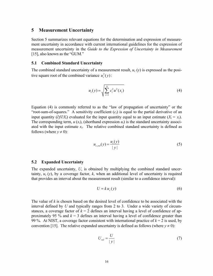
5 Measurement Uncertainty

Section 5 summarizes relevant equations for the determination and expression of measure-ment uncertainty in accordance with current international guidelines for the expression of measurement uncertainty in the Guide to the Expression of Uncertainty in Measurement [15], also known as the “GUM.”

5.1 Combined Standard Uncertainty The combined standard uncertainty of a measurement result, uc (y) is expressed as the posi-tive square root of the combined variance 2 ( )cu y :

2 2

1( ) ( )

N

c i ii

u y c u x=

= ∑ (4)

Equation (4) is commonly referred to as the “law of propagation of uncertainty” or the “root-sum-of-squares.” A sensitivity coefficient (ci) is equal to the partial derivative of an input quantity (∂f/∂Xi) evaluated for the input quantity equal to an input estimate (Xi = xi). The corresponding term, u (xi), (shorthand expression ui) is the standard uncertainty associ-ated with the input estimate xi. The relative combined standard uncertainty is defined as follows (where y ≠ 0):

,( )( )

| |c

c relu yu y

y= (5)

5.2 Expanded Uncertainty The expanded uncertainty, U, is obtained by multiplying the combined standard uncer-tainty, uc (y), by a coverage factor, k, when an additional level of uncertainty is required that provides an interval about the measurement result (similar to a confidence interval):

( )cU k u y= (6)

The value of k is chosen based on the desired level of confidence to be associated with the interval defined by U and typically ranges from 2 to 3. Under a wide variety of circum-stances, a coverage factor of k = 2 defines an interval having a level of confidence of ap-proximately 95 % and k = 3 defines an interval having a level of confidence greater than 99 %. At NIST, a coverage factor consistent with international practice of k = 2 is used, by convention [15]. The relative expanded uncertainty is defined as follows (where y ≠ 0):

| |relUUy

= (7)

17

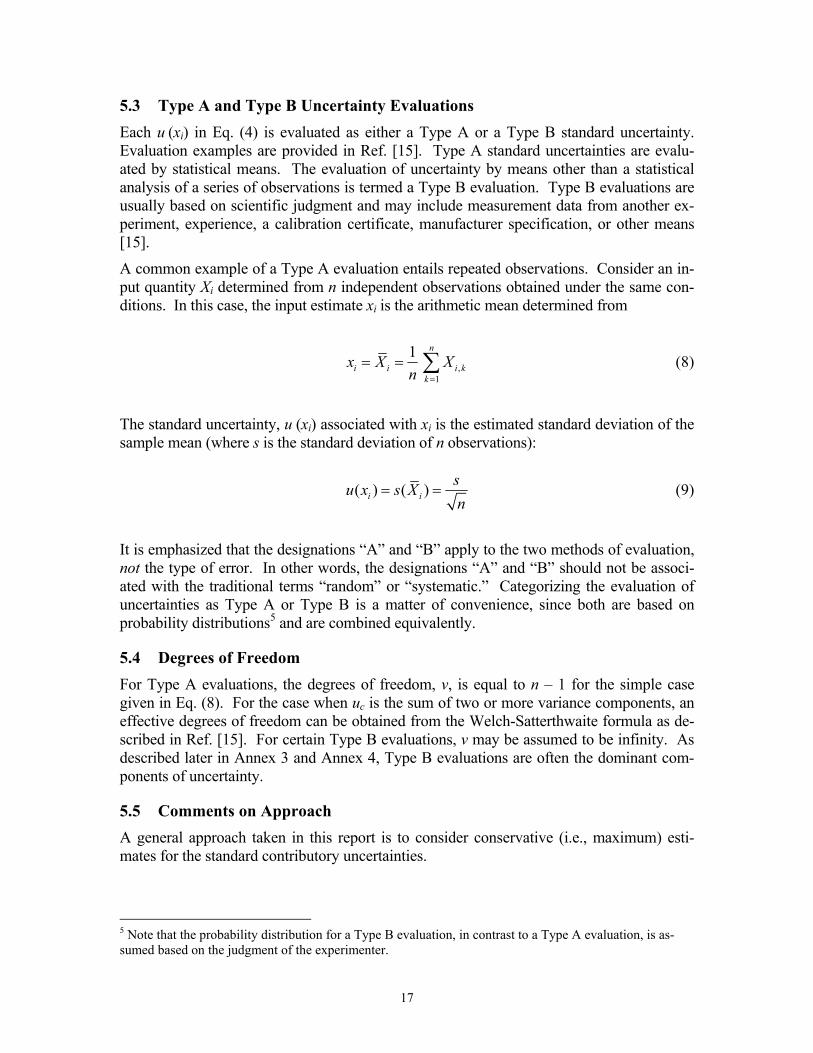
5.3 Type A and Type B Uncertainty Evaluations Each u (xi) in Eq. (4) is evaluated as either a Type A or a Type B standard uncertainty. Evaluation examples are provided in Ref. [15]. Type A standard uncertainties are evalu-ated by statistical means. The evaluation of uncertainty by means other than a statistical analysis of a series of observations is termed a Type B evaluation. Type B evaluations are usually based on scientific judgment and may include measurement data from another ex-periment, experience, a calibration certificate, manufacturer specification, or other means [15].

A common example of a Type A evaluation entails repeated observations. Consider an in-put quantity Xi determined from n independent observations obtained under the same con-ditions. In this case, the input estimate xi is the arithmetic mean determined from

,1

1 n

i i i kk

x X Xn =

= = ∑ (8)

The standard uncertainty, u (xi) associated with xi is the estimated standard deviation of the sample mean (where s is the standard deviation of n observations):

( ) ( )i isu x s Xn

= = (9)

It is emphasized that the designations “A” and “B” apply to the two methods of evaluation, not the type of error. In other words, the designations “A” and “B” should not be associ-ated with the traditional terms “random” or “systematic.” Categorizing the evaluation of uncertainties as Type A or Type B is a matter of convenience, since both are based on probability distributions5 and are combined equivalently.

5.4 Degrees of Freedom For Type A evaluations, the degrees of freedom, v, is equal to n – 1 for the simple case given in Eq. (8). For the case when uc is the sum of two or more variance components, an effective degrees of freedom can be obtained from the Welch-Satterthwaite formula as de-scribed in Ref. [15]. For certain Type B evaluations, v may be assumed to be infinity. As described later in Annex 3 and Annex 4, Type B evaluations are often the dominant com-ponents of uncertainty.

5.5 Comments on Approach A general approach taken in this report is to consider conservative (i.e., maximum) esti-mates for the standard contributory uncertainties.

5 Note that the probability distribution for a Type B evaluation, in contrast to a Type A evaluation, is as-sumed based on the judgment of the experimenter.

18

6 Bulk Density Study

Section 6 describes the measurements of mass and linear dimensions for the determina-tion of bulk density of an insulation panel. Graphical analyses and tabulated results for mass, panel area, thickness, and bulk density for all 450 specimens are presented.

6.1 Panel Mass Measurements The mass measurement of the insulation panel is based on the gravimetric method. The measurement station consisted of the following equipment: a) digital weighing balance (32.1 kg range, 0.0001 kg resolution); b) foot switch for manual event activation; and, c) RS-232 serial interface for the balance and a desktop computer.

Each sample of 50 insulation panels was placed collectively in a large convection oven at 100 °C and conditioned overnight for approximately 20 h. The panels were removed from the oven, one by one, and weighed as a function of time. The start time (t0) was synchronized with removal by activation of the foot switch. The mass data (in kilo-grams) were acquired from the digital balance every 20 s for 180 s (3 min) using a com-puter program. When placed in ambient conditions, the insulation panel (re-) gains mass immediately due to the difference in relative humidity between the 100 °C environment and ambient air. By measuring the panel mass at equal time intervals and establishing a mass history, the initial mass (m0) for each panel at time zero (t0) is determined by regres-sion analysis, thus correcting for the small mass change with time.

The mass data at time (t) were fitted to Eq. (10) using three different computer analysis programs, cross-checked for complete consistency of results.

( ) 0m t m a t= + (10)

Annex 1 provides a graphical analysis of the mass measurements for all 450 insulation panels and summarizes regression values for m0 for each panel.

Figure 1 illustrates the typical mass regain data for an insulation panel (438). The indi-vidual observations, shown as diamond symbols, are plotted with error bars representing an expanded uncertainty (k = 2) of 0.00012 kg. The linear fit for the data is shown as a solid line. The initial mass (m0) of 1.1060 kg was determined by linear back-extrapolation (dashed line extension in Fig. 1) to time t0. The mass regain for an insula-tion panel over the time interval of 180 s was typically about 0.1 %.

6.2 Dimensional Measurements The dimensional measurements are derived from one-dimensional length measurements using precision electronic height gages referenced to a surface plate datum. The height gages were placed on, and referenced to, a granite surface plate having linear dimensions of 1.2 m by 1.8 m and a unilateral flatness tolerance of 0.018 mm. Each height gage util-ized a touch signal probe that provided a consistent contact force with the artifact. The length value (in millimeters) was transferred to a desktop computer with a USB (Univer-sal Serial Bus) interface cable and recorded in an electronic spreadsheet template. The length, width, and thickness measurements of each group of 50 insulation panels were

19

1.1055

1.1060

1.1065

1.1070

1.1075

1.1080

0 20 40 60 80 100 120 140 160 180 200Elapsed time, s

Mas

s, k

g

Figure 1. Mass regain for Panel ID 438 after removal of panel from oven. Initial mass (m0) of 1.1060 kg was determined by linear extrapolation to time zero.

performed at the same time by two operators under ambient conditions of approximately 23 °C and 35 % relative humidity.

6.2.1 Lateral Panel Dimensions – Length and Width Figure 2 illustrates the essential details for measurement of the panel lateral dimensions (length and width). The measurement station consists of the following instrumentation:

a. granite surface plate (1.2 m by 1.8 m, unilateral flatness tolerance of 0.018 mm); b. electronic height gage with digital readout (635 mm range, 0.01 mm resolution); c. bi-directional touch probe (3 mm diameter carbide ball contact point, 0.4 N

measuring force); and, d. SPC (statistical process control) data output cable with converter tool to USB

(Universal Serial Bus) communication cable for connection to a desktop com-puter.

The insulation panel was placed on edge, in the vertical position, on the granite surface plate and clamped securely between an aluminum sheet and a right-angle support fixture (Fig. 2a). The fixture consisted of an aluminum jig plate (13 mm thick by 560 mm 560 mm) fastened to two precision ground right angles (200 mm by 125 mm). The right angles were precision ground square to within 0.051 mm (per 150 mm) and parallel to within 0.006 mm (per 150 mm). The touch probe measurements were carried out with a round high-grade gage block as the workpiece (in contact with the insulation panel).

20

Figure 2. a) Side view shows 610 mm height gage and right-angle fixture with insulation panel clamped between the aluminum jig plate and aluminum sheet. b) Front view shows panel length measurements at locations l1, l2, l3, l4, l5, and l6 (fixture and height gage are not shown). For a particular group of 50 panels, one panel was measured at all locations and the other 49 panels were measured at locations l2 and l5.

Linear dimensions l1, l2, and l3 were obtained by moving the height gage and measuring at the three locations. The panel was subsequently unclamped, rotated 90° clockwise, and re-clamped to measure linear dimensions l4, l5, and l6. Preliminary tests indicated that data acquired from two middle locations, l2 and l5, were sufficient for the accurate determination of bulk density. As a check, however, one panel from each group was se-lected, at random, for measurements at all locations (l1, l2, l3, l4, l5, and l6).

After completion of the mass measurements (Sec. 6.1), the group of 50 panels was placed collectively in a laboratory ambient of 23 °C and conditioned overnight for about 17 h. Prior to dimensional measurements, a zero reference plane for the workpiece with respect to the surface datum, was established. The measurement process was checked at the be-ginning and end using a 609.6 mm gage standard consisting of two 304.8 mm gage blocks wrung together. During the measurement process, the zero reference plane was re-established, as necessary. For 49 panels, the linear dimensions l2 and l5 were obtained. For one panel, selected at random from each group, the linear dimension measurements were conducted at l1, l2, l3, l4, l5, and l6.

For nine panels, one from each group of 50 (Panel ID: 048, 110, 173, 298, 336, 348, 350, 392, and 408), the area of the panel As was computed using Eq. (11).

1 2 3 4 5 6

3 3sl l l l l lA + + + +⎛ ⎞ ⎛ ⎞= ×⎜ ⎟ ⎜ ⎟

⎝ ⎠ ⎝ ⎠ (11)

5

b)

l1 l2 l3

l6

l5

l4

4

1) Height gage 2) Touch probe 3) SPC output 4) Workpiece 5) Insulation panel 6) Granite surface plate7) Right-angle fixture

a)

3 2

1

7

6

21

The areas (As) of the other panels were computed using Eq. (12).

2 5sA l l= × (12)

6.2.2 Thickness Figure 3 illustrates the essential details for measurement of the panel thickness dimen-sions. The measurement station consists of the following equipment and instrumentation:

a. granite surface plate (1.2 m by 1.8 m, unilateral flatness tolerance of 0.018 mm); b. electronic height gage with digital readout (330 mm range, 0.01 mm resolution); c. bi-directional touch probe (3 mm diameter carbide ball contact point, 0.4 N meas-

uring force); and, d. SPC (statistical process control) data output cable with converter tool to USB

(Universal Serial Bus) communication cable for connection to a desktop com-puter.

Figure 3. a) Front view shows 305 mm height gage and insulation panel (with workpiece) on granite sur-face plate. b) Top view shows an insulation panel and 8 thickness measurement locations (L1 – L8) each in the geometric center of a 200 mm by 200 mm sub-area of the insulation panel. For a particular group of 50 panels, one panel was measured at all 8 locations and the other 49 panels were measured, in an alternating sequence, at the corner locations (L1, L3, L5, L7) and at the mid-center locations (L2, L4, L6, L8).

The insulation panel was placed, in the horizontal position, on the granite surface plate (Fig. 3a) and a modest load (approximately 43 N, not shown in Fig. 3a) was applied to the top of the panel. The panel thickness was measured at 8 locations (L1, L2, L3, L4, L5, L6, L7, and L8 as shown in Fig. 3b); each location representing the geometric center of a 200 mm by 200 mm sub-area. The touch probe measurements were carried out with a round high-grade gage block as the workpiece in contact with the insulation panel (Fig. 3a).

b)

L1

L2

L3 L4 L5

L6

L7 L8

200 mm

200 mm

1) Height gage 2) Touch probe 3) SPC output 4) Workpiece 5) Insulation panel 6) Granite surface plate

1

a)

6 5 4

2 3

22

The linear dimensions L1, L2, L3, L4, L5, L6, L7, and L8 were obtained by fixing the loca-tion of the height gage (in contrast to the lateral dimensional measurements where the height gage was moved from location to location) and re-positioning the panel for each measurement. Preliminary tests indicated that the data acquired from four locations were sufficient for an accurate determination of the bulk density. For each group, approxi-mately one-half of the panels were measured at the corners (L1, L3, L5, and L7) and, for the other half, at the mid-centers (L2, L4, L6, and L8). The measurement pattern was alter-nated from panel to panel.

The thickness measurements were conducted by a second operator at the same time that the lateral panel dimensions (Sec. 6.2.1) were collected. Prior to dimensional measure-ments, a zero reference plane for the workpiece with respect to the surface datum, was established. The measurement process was checked at the beginning and end using a 25.4 mm (1 in.) gage block standard. During the measurement process, the zero refer-ence plane was re-established, as necessary. For 49 panels, the linear dimensions at the corners (L1, L3, L5, and L7) and at the mid-centers (L2, L4, L6, and L8) were obtained. For one panel, selected at random from the group, the linear dimension measurements were conducted at L1, L2, L3, L4, L5, L6, L7, and L8.

For nine panels, one from each group of 50 (Panel ID: 048, 110, 173, 298, 336, 348, 350, 392, and 408), the mean thickness of the panel was computed using Eq. (13). The thick-nesses of the other panels were computed using either Eq. (14) or Eq. (15).

( )1 2 3 4 5 6 7 8 8mL L L L L L L L L= + + + + + + + (13)

( )1 3 5 7 4mL L L L L= + + + (14)

( )2 4 6 8 4mL L L L L= + + + (15)

Annex 2 provides a graphical analysis of the thickness measurements for all 450 insula-tion panels.

6.3 Homogeneity Assessment

6.3.1 Tabulated Results The following data were collected over a 30 day period.

– 4050 mass measurements (9 points per panel × 450 panels) – 936 lateral panel dimensions (2 per panel × 441 panels + 6 per panel × 9 panels) – 1836 thickness dimensions (4 per panel × 441 panels + 8 per panel × 9 panels)

Table 3 summarizes mass (m0), length (l2), width (l5), area (As), thickness (Lm), and bulk density (ρ) for the 450 panels. The bulk density for each panel was determined using Eq. (1) and the values presented in Table 3 were rounded to the nearest whole number for certification purposes.

23

Table 3. Physical properties of SRM 1450d units (450 panels)

Panel ID Mass (kg)

Length (mm)

Width (mm)

Area (m2)

Thickness (mm)

Bulk density (kg·m-3)

001 1.12414 611.24 610.08 0.37291 25.93 116 002 1.13986 611.11 611.77 0.37386 25.94 118 003 1.11269 610.96 610.07 0.37273 25.68 116 004 1.18653 611.04 611.53 0.37367 25.81 123 005 1.17210 611.10 610.21 0.37290 25.83 122 006 1.13738 610.67 611.33 0.37332 25.63 119 007 1.16968 610.11 611.11 0.37284 25.95 121 008 1.15530 611.82 611.07 0.37386 25.85 120 009 1.18189 610.19 610.51 0.37253 25.74 123 010 1.15906 611.96 610.53 0.37362 25.71 121 011 1.16495 610.10 610.80 0.37265 25.78 121 012 1.16937 611.55 610.50 0.37335 25.60 122 013 1.14597 610.37 610.54 0.37266 26.10 118 014 1.12582 611.42 610.63 0.37335 25.95 116 015 1.11244 610.25 610.75 0.37271 25.83 116 016 1.18237 611.47 611.21 0.37374 25.88 122 017 1.12531 610.15 611.20 0.37292 25.88 117 018 1.12734 611.72 611.15 0.37385 25.70 117 019 1.18564 610.86 610.00 0.37262 26.02 122 020 1.12829 610.88 611.76 0.37371 25.95 116 021 1.17589 610.66 610.20 0.37262 25.83 122 022 1.14641 610.73 611.53 0.37348 25.86 119 023 1.13887 611.10 609.78 0.37264 25.87 118 024 1.13869 610.90 611.80 0.37375 25.76 118 025 1.14179 611.35 610.16 0.37302 25.94 118 026 1.16275 610.88 611.88 0.37379 25.95 120 027 1.19277 611.04 610.27 0.37290 25.80 124 028 1.17184 610.57 611.61 0.37343 25.74 122 029 1.19291 611.20 610.20 0.37295 25.92 123 030 1.16272 611.00 611.61 0.37369 25.72 121 031 1.13741 610.35 610.62 0.37269 26.07 117 032 1.11931 611.76 610.89 0.37372 25.95 115 033 1.16243 610.25 610.56 0.37259 25.82 121 034 1.16647 611.62 610.64 0.37348 25.85 121 035 1.14204 610.27 610.75 0.37272 25.81 119 036 1.17069 611.90 610.54 0.37359 25.67 122 037 1.12064 610.29 610.72 0.37272 25.62 117 038 1.13265 611.47 610.50 0.37330 25.65 118 039 1.13734 610.23 610.94 0.37281 25.25 121 040 1.17376 611.81 610.66 0.37361 25.49 123 041 1.17620 610.24 610.82 0.37275 25.58 123 042 1.16396 611.89 611.03 0.37388 25.49 122 043 1.10074 610.42 609.81 0.37224 26.17 113 044 1.09948 610.98 611.68 0.37372 26.08 113 045 1.16567 610.71 609.85 0.37244 25.83 121 046 1.17663 611.13 612.17 0.37412 25.98 121 047 1.15239 610.77 609.93 0.37253 25.92 119 048 1.16201 610.63 611.97 0.37369 25.69 121 049 1.13219 611.11 610.23 0.37292 26.40 115 050 1.14569 610.89 611.79 0.37374 26.29 117 051 1.15778 610.90 610.13 0.37273 26.03 119 052 1.13913 610.66 611.66 0.37352 26.12 117 053 1.15072 611.19 610.25 0.37298 26.13 118 054 1.14068 611.12 611.50 0.37370 25.98 117

24

Panel ID Mass (kg)

Length (mm)

Width (mm)

Area (m2)

Thickness (mm)

Bulk density (kg·m-3)

055 1.07006 610.43 611.16 0.37307 26.12 110 056 1.12219 611.83 610.67 0.37363 26.07 115 057 1.15492 610.37 610.81 0.37282 25.90 120 058 1.15498 612.15 610.88 0.37395 25.93 119 059 1.16159 610.27 610.84 0.37278 25.87 120 060 1.21462 611.75 610.88 0.37371 25.81 126 061 1.10081 610.29 610.85 0.37280 26.13 113 062 1.12217 611.76 611.16 0.37388 26.08 115 063 1.15255 610.15 610.67 0.37260 25.75 120 064 1.18817 611.60 610.59 0.37344 25.95 123 065 1.11860 610.13 611.39 0.37303 25.95 116 066 1.16964 611.81 610.88 0.37374 25.85 121 067 1.14153 610.76 610.06 0.37260 26.14 117 068 1.14135 610.90 611.83 0.37377 26.10 117 069 1.14468 610.80 610.02 0.37260 25.76 119 070 1.11146 610.86 611.74 0.37369 25.82 115 071 1.16491 610.76 609.98 0.37255 25.91 121 072 1.12173 611.11 612.14 0.37408 25.92 116 073 1.12098 611.25 610.31 0.37305 26.17 115 074 1.15342 611.18 612.55 0.37438 26.08 118 075 1.16052 611.05 610.31 0.37293 25.84 120 076 1.16589 610.99 611.68 0.37373 25.86 121 077 1.15908 611.08 610.21 0.37289 25.84 120 078 1.16507 610.96 611.90 0.37385 25.79 121 079 1.13272 610.27 610.66 0.37267 26.03 117 080 1.14299 612.05 610.80 0.37384 25.98 118 081 1.14938 610.37 610.48 0.37262 25.73 120 082 1.15524 611.86 610.65 0.37363 25.81 120 083 1.12402 610.14 610.94 0.37276 25.78 117 084 1.14579 611.91 611.02 0.37389 25.81 119 085 1.11773 610.25 610.73 0.37270 26.28 114 086 1.12733 611.72 610.85 0.37367 26.10 116 087 1.14251 610.07 610.72 0.37258 25.88 118 088 1.16444 611.63 611.43 0.37397 25.94 120 089 1.14362 610.34 610.90 0.37286 25.90 118 090 1.14858 612.35 611.02 0.37416 25.90 119 091 1.15353 610.99 609.96 0.37268 26.13 118 092 1.18182 610.54 612.06 0.37369 26.03 122 093 1.19095 610.68 610.08 0.37256 25.75 124 094 1.13556 610.81 611.67 0.37361 25.83 118 095 1.15624 610.80 609.94 0.37255 25.81 120 096 1.13250 610.98 611.86 0.37383 25.79 117 097 1.13910 611.21 610.54 0.37317 26.12 117 098 1.14081 610.66 611.82 0.37361 26.04 117 099 1.13039 611.17 610.29 0.37299 25.87 117 100 1.18780 611.00 611.83 0.37383 25.95 122 101 1.14089 611.27 610.26 0.37303 25.91 118 102 1.15616 610.78 611.69 0.37361 25.82 120 103 1.10762 610.11 610.88 0.37270 26.18 114 104 1.13218 611.47 611.15 0.37370 26.04 116 105 1.16749 610.22 610.50 0.37254 25.84 121 106 1.14976 611.81 610.56 0.37355 25.96 119 107 1.15366 610.15 611.23 0.37294 26.02 119 108 1.15410 611.51 610.89 0.37357 25.83 120 109 1.15485 610.21 610.46 0.37251 26.21 118 110 1.12173 611.41 610.48 0.37326 25.98 116 111 1.13179 610.26 610.57 0.37261 25.82 118

25

Panel ID Mass (kg)

Length (mm)

Width (mm)

Area (m2)

Thickness (mm)

Bulk density (kg·m-3)

112 1.17517 611.55 610.69 0.37347 25.90 122 113 1.15025 610.26 610.46 0.37254 25.97 119 114 1.13912 611.44 611.14 0.37368 25.80 118 115 1.07447 610.85 610.08 0.37267 26.06 111 116 1.12192 610.63 611.94 0.37367 26.03 115 117 1.18546 610.90 610.04 0.37267 25.83 123 118 1.18503 610.57 611.38 0.37329 25.92 122 119 1.13788 609.96 611.30 0.37287 25.95 118 120 1.17795 610.74 611.84 0.37368 25.85 122 121 1.14709 611.32 610.40 0.37315 26.10 118 122 1.16647 610.99 611.65 0.37371 26.04 120 123 1.15868 610.98 610.16 0.37280 25.82 120 124 1.18168 610.91 611.67 0.37368 25.98 122 125 1.11063 610.97 610.25 0.37284 25.85 115 126 1.15448 610.97 611.87 0.37383 25.76 120 127 1.14412 610.25 610.32 0.37245 26.09 118 128 1.12675 611.78 611.02 0.37381 25.93 116 129 1.18062 610.33 610.54 0.37263 25.79 123 130 1.16665 611.63 611.08 0.37375 25.81 121 131 1.16387 610.31 610.78 0.37277 25.87 121 132 1.13133 611.54 611.15 0.37374 25.74 118 133 1.15076 610.09 610.64 0.37255 26.22 118 134 1.10108 611.70 611.02 0.37376 26.07 113 135 1.13652 610.29 610.62 0.37266 26.05 117 136 1.16872 611.61 610.52 0.37340 26.10 120 137 1.14970 610.41 611.10 0.37302 26.08 118 138 1.10254 611.65 611.06 0.37375 25.94 114 139 1.13972 610.68 609.88 0.37244 26.10 117 140 1.14971 610.51 611.62 0.37340 25.99 118 141 1.16087 610.61 609.84 0.37237 25.74 121 142 1.19183 610.71 611.51 0.37346 25.89 123 143 1.18258 610.86 610.08 0.37267 25.87 123 144 1.16138 610.36 611.56 0.37327 25.76 121 145 1.15147 611.20 610.38 0.37306 26.08 118 146 1.06968 610.94 610.89 0.37322 25.94 110 147 1.14651 611.07 610.42 0.37301 25.77 119 148 1.14698 611.21 611.76 0.37391 25.84 119 149 1.12615 611.43 610.29 0.37315 25.88 117 150 1.11505 610.98 611.79 0.37379 25.79 116 151 1.10047 610.65 610.68 0.37291 26.04 113 152 1.11863 611.41 610.91 0.37352 26.02 115 153 1.14852 610.47 610.78 0.37286 25.83 119 154 1.12696 611.56 610.83 0.37356 25.76 117 155 1.15228 610.45 610.82 0.37288 25.98 119 156 1.14876 611.74 610.88 0.37370 25.83 119 157 1.12336 611.63 611.17 0.37381 26.58 113 158 1.15833 611.64 610.35 0.37331 26.99 115 159 1.13203 611.82 611.07 0.37386 26.70 113 160 1.15569 610.28 610.94 0.37284 26.66 116 161 1.13572 610.22 611.05 0.37287 26.43 115 162 1.10457 611.90 610.80 0.37375 26.04 113 163 1.11441 610.51 610.34 0.37262 26.09 115 164 1.12297 610.79 611.72 0.37363 25.95 116 165 1.21054 610.57 610.06 0.37248 25.86 126 166 1.13067 610.89 611.72 0.37369 25.82 117 167 1.23314 610.75 610.03 0.37258 25.90 128 168 1.14794 610.72 611.67 0.37356 25.82 119

26

Panel ID Mass (kg)

Length (mm)

Width (mm)

Area (m2)

Thickness (mm)

Bulk density (kg·m-3)

169 1.11604 611.08 610.04 0.37278 26.13 115 170 1.12881 611.21 611.53 0.37377 26.04 116 171 1.14443 611.10 610.38 0.37300 25.94 118 172 1.13193 610.70 611.75 0.37360 25.83 117 173 1.11926 611.20 610.32 0.37303 25.89 116 174 1.12596 610.88 611.79 0.37373 25.75 117 175 1.11408 610.34 610.89 0.37285 26.18 114 176 1.10366 612.22 610.76 0.37392 26.04 113 177 1.16187 610.09 611.11 0.37283 25.92 120 178 1.14571 611.76 611.10 0.37385 25.95 118 179 1.15042 610.30 611.11 0.37296 26.06 118 180 1.17077 611.57 611.04 0.37369 25.91 121 181 1.14671 610.15 610.52 0.37251 26.22 117 182 1.08920 611.97 610.98 0.37390 25.96 112 183 1.15781 610.12 610.74 0.37262 25.82 120 184 1.14512 611.60 610.69 0.37350 25.88 118 185 1.20018 610.11 610.83 0.37267 25.90 124 186 1.10256 611.58 611.02 0.37369 25.80 114 187 1.14518 610.44 609.89 0.37230 26.16 118 188 1.10250 611.26 611.94 0.37405 26.00 113 189 1.15670 610.89 610.17 0.37275 25.82 120 190 1.15145 610.82 611.67 0.37362 25.96 119 191 1.15948 610.54 609.92 0.37238 25.88 120 192 1.20685 610.75 611.47 0.37346 25.86 125 193 1.13247 611.05 610.24 0.37289 25.97 117 194 1.07868 610.81 612.00 0.37382 25.97 111 195 1.14213 610.96 610.28 0.37286 25.77 119 196 1.10984 610.79 611.52 0.37351 25.84 115 197 1.11919 611.23 610.12 0.37292 25.89 116 198 1.15352 611.00 611.70 0.37375 25.76 120 199 1.12973 610.25 611.11 0.37293 26.35 115 200 1.10731 611.76 610.82 0.37368 26.23 113 201 1.12089 610.26 610.67 0.37267 26.00 116 202 1.13515 611.49 610.84 0.37352 25.95 117 203 1.18179 610.09 610.64 0.37255 25.98 122 204 1.13426 611.50 610.94 0.37359 25.74 118 205 1.11970 610.18 610.81 0.37270 26.16 115 206 1.08548 612.21 610.73 0.37390 26.04 111 207 1.11356 610.36 610.53 0.37264 25.86 116 208 1.14218 611.67 610.87 0.37365 25.92 118 209 1.14201 610.35 611.11 0.37299 25.90 118 210 1.16556 611.76 610.54 0.37350 25.82 121 211 1.13124 610.92 610.07 0.37270 26.05 117 212 1.12840 610.71 611.80 0.37363 26.01 116 213 1.16842 610.56 610.08 0.37249 25.88 121 214 1.14418 610.80 611.64 0.37359 25.84 119 215 1.16701 611.03 610.21 0.37286 25.96 121 216 1.10545 610.63 611.42 0.37335 25.80 115 217 1.12624 611.08 610.10 0.37282 26.10 116 218 1.12680 610.92 611.79 0.37375 25.92 116 219 1.15334 610.89 610.38 0.37288 25.82 120 220 1.15179 610.85 611.71 0.37366 25.92 119 221 1.17024 611.06 610.15 0.37284 25.87 121 222 1.09915 610.99 611.83 0.37382 25.73 114 223 1.15226 610.46 610.64 0.37277 26.06 119 224 1.12542 612.11 610.97 0.37398 25.88 116 225 1.15646 610.39 610.89 0.37288 25.76 120

27

Panel ID Mass (kg)

Length (mm)

Width (mm)

Area (m2)

Thickness (mm)

Bulk density (kg·m-3)

226 1.16833 611.62 610.74 0.37354 25.77 121 227 1.12953 610.22 610.91 0.37279 25.79 117 228 1.13737 611.66 611.07 0.37377 25.68 118 229 1.14301 610.16 610.69 0.37262 26.03 118 230 1.12638 611.96 610.75 0.37375 25.88 116 231 1.16284 610.27 610.84 0.37278 25.71 121 232 1.20029 611.90 610.51 0.37357 25.77 125 233 1.16669 610.13 610.83 0.37269 25.75 122 234 1.13291 612.06 610.89 0.37390 25.70 118 235 1.16433 610.82 610.25 0.37275 26.02 120 236 1.15741 610.88 611.63 0.37363 25.89 120 237 1.18919 610.55 609.98 0.37242 25.67 124 238 1.15449 611.01 611.71 0.37376 25.70 120 239 1.13509 610.38 610.41 0.37258 25.76 118 240 1.18396 610.77 611.42 0.37344 25.65 124 241 1.11091 610.78 610.14 0.37266 26.01 115 242 1.10286 610.87 612.05 0.37388 25.80 114 243 1.16182 611.28 610.48 0.37317 25.73 121 244 1.17091 611.09 611.69 0.37380 25.67 122 245 1.18471 610.80 610.16 0.37269 25.91 123 246 1.18464 611.04 611.68 0.37376 25.69 123 247 1.13150 610.43 610.70 0.37279 26.02 117 248 1.13631 612.00 610.77 0.37379 25.81 118 249 1.11462 610.13 611.00 0.37279 25.72 116 250 1.13862 611.82 610.85 0.37373 25.76 118 251 1.11650 610.21 610.70 0.37266 25.81 116 252 1.15906 611.57 610.73 0.37350 25.62 121 253 1.13919 610.26 610.93 0.37283 25.96 118 254 1.10615 612.10 610.92 0.37394 25.76 115 255 1.16429 610.26 610.76 0.37272 25.70 122 256 1.14729 611.63 611.09 0.37376 25.81 119 257 1.13116 610.21 610.78 0.37270 25.74 118 258 1.15010 611.82 610.78 0.37369 25.65 120 259 1.12227 610.22 611.04 0.37287 26.04 116 260 1.07708 612.02 610.89 0.37388 25.88 111 261 1.15488 610.16 610.90 0.37275 25.77 120 262 1.15963 611.73 610.82 0.37366 25.78 120 263 1.12172 610.26 611.31 0.37306 25.86 116 264 1.12846 611.91 610.70 0.37369 25.83 117 265 1.13800 611.21 610.46 0.37312 25.99 117 266 1.12327 610.84 612.10 0.37390 25.82 116 267 1.14465 611.12 610.47 0.37307 25.65 120 268 1.14092 610.95 611.77 0.37376 25.59 119 269 1.15724 611.18 610.23 0.37296 25.79 120 270 1.14636 610.79 611.67 0.37360 25.59 120 271 1.14040 610.27 610.60 0.37263 25.97 118 272 1.15038 611.86 611.02 0.37386 25.78 119 273 1.16056 610.22 610.90 0.37278 25.63 121 274 1.13994 611.84 610.71 0.37366 25.67 119 275 1.13412 610.26 611.11 0.37294 25.81 118 276 1.14093 611.76 611.14 0.37387 25.53 120 277 1.15168 610.14 610.85 0.37270 26.27 118 278 1.16131 611.68 611.01 0.37374 25.96 120 279 1.17856 610.36 610.75 0.37278 25.89 122 280 1.15230 611.73 610.72 0.37360 25.75 120 281 1.16368 610.33 611.33 0.37311 26.02 120 282 1.11690 611.63 611.33 0.37391 25.64 116

28

Panel ID Mass (kg)

Length (mm)

Width (mm)

Area (m2)

Thickness (mm)

Bulk density (kg·m-3)

283 1.12053 611.02 609.99 0.37272 25.91 116 284 1.12628 610.83 611.87 0.37375 25.82 117 285 1.12822 610.77 609.85 0.37248 25.63 118 286 1.14708 610.83 611.84 0.37373 25.67 120 287 1.13461 611.09 610.06 0.37280 25.82 118 288 1.14216 611.01 611.75 0.37379 25.68 119 289 1.16081 610.55 610.17 0.37254 25.91 120 290 1.15201 610.70 611.73 0.37358 25.83 119 291 1.18236 611.02 610.23 0.37286 25.66 124 292 1.20610 610.93 611.97 0.37387 25.58 126 293 1.18124 611.13 610.29 0.37297 25.73 123 294 1.19497 610.86 611.82 0.37374 25.58 125 295 1.11555 610.76 610.91 0.37312 25.90 115 296 1.12221 611.64 610.97 0.37369 25.83 116 297 1.16962 610.24 611.00 0.37286 25.68 122 298 1.12113 611.60 610.38 0.37331 25.68 117 299 1.18001 610.25 610.66 0.37266 25.89 122 300 1.15708 611.65 610.74 0.37356 25.85 120 301 1.13965 610.51 611.21 0.37315 25.93 118 302 1.16369 612.01 611.01 0.37394 25.83 120 303 1.15664 610.32 610.25 0.37245 25.69 121 304 1.17066 611.83 610.78 0.37369 25.58 122 305 1.15275 610.24 611.14 0.37294 25.77 120 306 1.15196 611.65 610.86 0.37363 25.59 121 307 1.11287 610.30 610.71 0.37272 26.01 115 308 1.11155 611.96 610.65 0.37369 25.78 115 309 1.18160 610.41 610.92 0.37291 25.71 123 310 1.13664 612.17 611.08 0.37408 25.64 119 311 1.17607 610.21 611.13 0.37292 25.78 122 312 1.14976 611.76 610.96 0.37376 25.59 120 313 1.11391 611.57 610.32 0.37325 26.17 114 314 1.12859 611.34 611.88 0.37407 25.82 117 315 1.13903 611.49 610.20 0.37313 25.83 118 316 1.15524 611.34 611.82 0.37403 25.59 121 317 1.14585 610.89 610.32 0.37284 25.83 119 318 1.14134 611.06 612.28 0.37414 25.58 119 319 1.12044 610.47 610.83 0.37289 25.97 116 320 1.14848 611.78 610.65 0.37358 25.74 119 321 1.13955 610.21 610.55 0.37256 25.59 120 322 1.18656 611.65 610.53 0.37343 25.58 124 323 1.14363 610.26 611.17 0.37297 25.71 119 324 1.12941 612.01 610.76 0.37379 25.58 118 325 1.12908 610.29 610.75 0.37273 26.04 116 326 1.11530 611.60 611.10 0.37375 25.77 116 327 1.14984 611.54 611.00 0.37365 25.54 121 328 1.17150 610.14 610.73 0.37263 25.74 122 329 1.15462 610.38 610.87 0.37286 25.83 120 330 1.19245 611.63 610.96 0.37368 25.61 125 331 1.11002 610.89 610.02 0.37266 26.06 114 332 1.11409 611.02 612.06 0.37398 25.92 115 333 1.15996 610.80 610.08 0.37264 25.85 120 334 1.14948 611.01 611.76 0.37379 25.70 120 335 1.14968 610.86 610.03 0.37264 25.81 120 336 1.14833 610.84 611.47 0.37351 25.62 120 337 1.11168 610.72 611.36 0.37337 25.96 115 338 1.15613 610.39 611.28 0.37312 25.80 120 339 1.13794 610.92 611.66 0.37368 25.58 119

29

Panel ID Mass (kg)

Length (mm)

Width (mm)

Area (m2)

Thickness (mm)

Bulk density (kg·m-3)

340 1.16806 610.69 609.96 0.37250 25.74 122 341 1.13174 610.79 611.57 0.37354 25.54 119 342 1.20857 610.65 610.36 0.37272 25.81 126 343 1.19092 610.40 610.41 0.37259 25.93 123 344 1.16103 611.26 610.19 0.37298 25.78 121 345 1.15199 610.32 610.80 0.37278 25.61 121 346 1.15974 611.72 610.63 0.37353 25.55 122 347 1.16944 610.50 611.16 0.37311 25.75 122 348 1.16051 611.18 611.28 0.37360 25.56 122 349 1.14241 611.63 610.82 0.37360 25.83 118 350 1.15930 610.26 609.55 0.37198 25.87 120 351 1.18083 610.25 610.24 0.37240 25.63 124 352 1.19973 611.55 609.96 0.37302 25.66 125 353 1.18032 610.39 610.64 0.37273 25.73 123 354 1.18271 611.57 610.49 0.37336 25.59 124 355 1.15426 610.79 610.41 0.37283 25.91 119 356 1.14209 610.83 612.08 0.37388 25.82 118 357 1.15940 611.05 611.66 0.37375 25.68 121 358 1.14864 610.96 610.10 0.37275 25.73 120 359 1.12883 611.01 610.12 0.37279 25.87 117 360 1.14216 611.88 610.73 0.37369 25.68 119 361 1.11953 609.67 610.82 0.37240 26.09 115 362 1.11271 611.24 610.51 0.37317 25.90 115 363 1.14569 609.75 611.44 0.37283 25.79 119 364 1.17146 611.11 610.95 0.37336 25.84 121 365 1.12071 609.71 610.97 0.37251 25.95 116 366 1.13998 611.40 610.46 0.37324 25.84 118 367 1.15645 609.99 610.12 0.37217 25.95 120 368 1.11160 611.07 610.36 0.37297 25.84 115 369 1.13781 609.95 610.70 0.37250 25.71 119 370 1.16704 611.77 610.96 0.37377 25.90 121 371 1.15589 610.19 610.62 0.37259 26.16 119 372 1.16458 611.56 610.41 0.37330 25.82 121 373 1.13037 611.43 610.70 0.37340 26.03 116 374 1.13509 610.36 610.36 0.37254 26.05 117 375 1.13933 611.77 610.37 0.37341 25.89 118 376 1.14735 610.42 610.73 0.37280 25.78 119 377 1.15165 610.18 610.75 0.37267 25.99 119 378 1.12077 611.74 611.05 0.37380 25.84 116 379 1.14561 609.56 610.59 0.37219 26.06 118 380 1.13070 611.18 610.51 0.37313 25.97 117 381 1.13951 611.27 610.89 0.37342 25.86 118 382 1.17555 609.72 611.21 0.37267 25.77 122 383 1.18423 609.92 611.06 0.37270 25.90 123 384 1.15178 611.18 611.12 0.37350 25.74 120 385 1.15335 609.62 610.46 0.37215 26.05 119 386 1.14326 611.54 610.47 0.37333 25.98 118 387 1.15922 609.72 611.07 0.37258 25.85 120 388 1.17616 611.36 610.84 0.37344 25.80 122 389 1.14528 609.85 610.92 0.37257 25.91 119 390 1.12592 611.51 611.04 0.37366 25.75 117 391 1.10491 611.78 610.31 0.37338 25.97 114 392 1.14697 610.11 610.11 0.37223 26.10 118 393 1.17312 610.86 611.68 0.37365 25.85 121 394 1.16409 610.31 610.41 0.37254 25.87 121 395 1.13563 611.41 610.52 0.37328 25.81 118 396 1.12737 610.42 610.32 0.37255 25.80 117

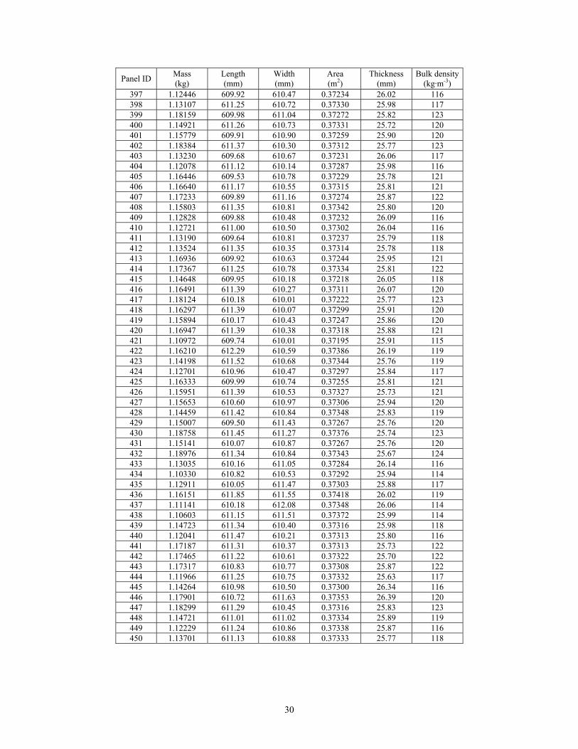
30

Panel ID Mass (kg)

Length (mm)

Width (mm)

Area (m2)

Thickness (mm)

Bulk density (kg·m-3)

397 1.12446 609.92 610.47 0.37234 26.02 116 398 1.13107 611.25 610.72 0.37330 25.98 117 399 1.18159 609.98 611.04 0.37272 25.82 123 400 1.14921 611.26 610.73 0.37331 25.72 120 401 1.15779 609.91 610.90 0.37259 25.90 120 402 1.18384 611.37 610.30 0.37312 25.77 123 403 1.13230 609.68 610.67 0.37231 26.06 117 404 1.12078 611.12 610.14 0.37287 25.98 116 405 1.16446 609.53 610.78 0.37229 25.78 121 406 1.16640 611.17 610.55 0.37315 25.81 121 407 1.17233 609.89 611.16 0.37274 25.87 122 408 1.15803 611.35 610.81 0.37342 25.80 120 409 1.12828 609.88 610.48 0.37232 26.09 116 410 1.12721 611.00 610.50 0.37302 26.04 116 411 1.13190 609.64 610.81 0.37237 25.79 118 412 1.13524 611.35 610.35 0.37314 25.78 118 413 1.16936 609.92 610.63 0.37244 25.95 121 414 1.17367 611.25 610.78 0.37334 25.81 122 415 1.14648 609.95 610.18 0.37218 26.05 118 416 1.16491 611.39 610.27 0.37311 26.07 120 417 1.18124 610.18 610.01 0.37222 25.77 123 418 1.16297 611.39 610.07 0.37299 25.91 120 419 1.15894 610.17 610.43 0.37247 25.86 120 420 1.16947 611.39 610.38 0.37318 25.88 121 421 1.10972 609.74 610.01 0.37195 25.91 115 422 1.16210 612.29 610.59 0.37386 26.19 119 423 1.14198 611.52 610.68 0.37344 25.76 119 424 1.12701 610.96 610.47 0.37297 25.84 117 425 1.16333 609.99 610.74 0.37255 25.81 121 426 1.15951 611.39 610.53 0.37327 25.73 121 427 1.15653 610.60 610.97 0.37306 25.94 120 428 1.14459 611.42 610.84 0.37348 25.83 119 429 1.15007 609.50 611.43 0.37267 25.76 120 430 1.18758 611.45 611.27 0.37376 25.74 123 431 1.15141 610.07 610.87 0.37267 25.76 120 432 1.18976 611.34 610.84 0.37343 25.67 124 433 1.13035 610.16 611.05 0.37284 26.14 116 434 1.10330 610.82 610.53 0.37292 25.94 114 435 1.12911 610.05 611.47 0.37303 25.88 117 436 1.16151 611.85 611.55 0.37418 26.02 119 437 1.11141 610.18 612.08 0.37348 26.06 114 438 1.10603 611.15 611.51 0.37372 25.99 114 439 1.14723 611.34 610.40 0.37316 25.98 118 440 1.12041 611.47 610.21 0.37313 25.80 116 441 1.17187 611.31 610.37 0.37313 25.73 122 442 1.17465 611.22 610.61 0.37322 25.70 122 443 1.17317 610.83 610.77 0.37308 25.87 122 444 1.11966 611.25 610.75 0.37332 25.63 117 445 1.14264 610.98 610.50 0.37300 26.34 116 446 1.17901 610.72 611.63 0.37353 26.39 120 447 1.18299 611.29 610.45 0.37316 25.83 123 448 1.14721 611.01 611.02 0.37334 25.89 119 449 1.12229 611.24 610.86 0.37338 25.87 116 450 1.13701 611.13 610.88 0.37333 25.77 118

31

6.3.2 Graphical Analyses Each quantity in Table 3 (mass, length, width, area, thickness, and bulk density) was sub-jected to a four-step graphical analysis to investigate the homogeneity of the material lot (i.e., between-panel results). For each set of data, the graphical analysis verified the under-lying assumptions of an ideal measurement process: a) stability (that is, fixed location and variation), b) randomness, and c) normality. It should be noted that initial diagnostic checks, using similar graphical data analyses (not presented), were applied to each group (50 panels) of data immediately after measurement completion to verify that measure-ment process was in control.

Figures 4-9 illustrate the four step graphical analysis for panel mass (m0), length (l2), width (l5), area (As), thickness (Lm), and bulk density (ρ), respectively, for the 450 panels. Each figure consists of 4 plots: a) run-sequence plot; b) lag plot; c) histogram; and d) normality plot. The four-step method was applied for verification of the four characteristics indicating statistical control of a process.

1) Run sequence plot plots values in the order obtained versus a sequence surrogate index (xi versus i) and checks for systematic and random changes.

2) Lag plot plots adjacent values (xi versus xi–1) and also checks for randomness (specifically, lack of autocorrelation).

3) A histogram of values (xi) checks the frequency distribution. 4) Normal probability plot of values (of xi) checks the normality assumption.

Diagnostic plots of the forms shown in Fig. 4-9, the so-called 4-plots, and in Annex 1 and Annex 2, were done throughout the data logging stages of the experiment to check the integrity of the data as the data were being taken, to check for outlying points or entire outlying samples, and to check that values – of m0, l2, l5, As, Lm, and resultant ρ – were within their anticipated ranges.

6.3.2.1 Panel Mass (m0) In Fig. 4 (m0), the run sequence shows no obvious drift or modulation. The lag plot shows no autocorrelation and both the histogram and normal (Gaussian) probability plot are compatible with a normality assumption for the data, with the possible exception of just a few of the tail (extreme end) points, which are routinely observed with empirical data.

6.3.2.2 Panel Length and Width (l2 and l5) In Fig. 5 and Fig. 6 (l2 and l5, respectively), there are suggestions of multimodality, that is, two or more underlying populations of lengths and widths, respectively. This is evident in the histograms (directly visible), the normal probability plots (multiple line segments with comparable slopes but different intercepts conjoined in a single plot), and even the run se-quence plots (high/low excursions from the mean values). The presence of multi-modes is almost certainly due simply to the fact that the boards are not quite square, so that pairs of sides do not match exactly in length. The lag sequence plots are not suggestive of any autocorrelation, or systematic departure from randomness.

32

+++ + +++ + +++ ++ +++ ++ + ++ ++ +++ +++ ++++ ++ + ++ + +++ +++ ++ + ++ ++ + +++ ++ ++ ++ +++ + ++ + ++++ +++ + ++ + ++ ++++++ ++ +++ + ++ ++ ++ ++ + + +++ + +++ +++ + +++ ++ + +++ + +++ ++++ + ++ + ++++ +++ ++ ++ ++ ++ ++ ++++ ++ +++ +++ ++++ ++ ++ ++ + ++ + + ++ + ++ ++++ + ++ ++ +++ +++ ++ +++ +++ ++ ++ +++ + +++ ++ ++++ ++ + +++ ++ ++ ++ ++ ++ +++ ++ ++ + +++ ++ ++ + +++ ++ + ++ + + ++ + ++ ++ + ++ +++ ++ ++ ++ + ++ ++ ++ ++++ + + ++ +++++ + + +++ ++ ++ ++ +++ + ++ ++ + ++ ++ +++ ++ + +++++ + +++ + ++ +++ ++++ + + + ++ +++ + ++ ++ ++ +++ + ++++ ++ + + ++ + + ++ ++ + + +++ ++ + +++ + + ++ ++ ++ +++++ + + + + +++ + ++++ + +++ ++ + + ++ + +++ + ++ + +++ ++ +

050

100

150

200

250

300

350

400

450

1.00

1.05

1.10

1.15

1.20

1.25

1.30

RU

N S

EQ

UE

NC

E

Inde

x

X, kg

++++ +++

+ ++ + ++ + +++ ++ +++ ++ ++++ + + ++ +++ ++ +++++ ++++ ++ +++ ++ ++ +++ ++ + ++ ++ ++ ++ + ++ +++ + +++ ++ + ++++ +++ + ++ ++ ++ + ++ + ++ + + ++ ++ + ++ ++ + ++ ++++ + + +++ +++ ++ +++ + ++ ++ ++ + ++ + + ++ + ++ +++ + ++ + ++++++ ++ + + ++ ++ + +++ ++ +++ +++ + + +++ ++++ ++ ++++ ++ + +++ + +++ +++ ++ ++ ++ +++ ++ + +++ ++ ++ ++ +++ +++ ++++ +++ +++ + +++ + ++ + ++ + ++ ++ + + + ++ + ++ ++ ++ ++ + ++ ++ + + ++ + ++ ++ +++ + ++ + + ++ ++ ++ +++ +++ + + +++ + ++ +++ ++ +++ ++ ++ + ++ ++ ++ ++ + + +++++ ++ ++ +++ ++ ++++ + ++ + ++ + ++ +++ + ++ +++ +++ + + +++ ++ + ++ + + ++++ + + + +++ +++ +++++ + + +++ + + +++ + ++ + ++ + + ++ ++ ++ ++ ++++ + ++ + ++++

1.00

1.05

1.10

1.15

1.20

1.25

1.30

1.00

1.05

1.10

1.15

1.20

1.25

1.30

LAG

PLO

T

X(i-

1), k

g

X, kg

0.9

1.0

1.1

1.2

1.3

0102030405060

HIS

TOG

RA

M

X, k

g

Frequency

++

+++++++++

+++++++++++++

+++++++++++++++++++++

+++++++++++++++++++++++++++++++

+++++++++++++++++++++++++ ++++++++++++++++++

+++++++++++++++++++++++++++++++++++++++++++++++++++++

++++++++++++++++++++++++++++++++ ++++++++++++++++++++++++++

++++++++++++++++++++++++++++++++++++++++++++++++++++++++++

+++++++++++++++++++++++ +++++++++++++++++++++++++++

++++++++++++++++++++++++++++++++++++++++++

++++++++++++++++++++++++++++++

++ ++++++++++++++++++

+++++++++++

+++++

+++

+

-3-2

-10

12

3

1.00

1.05

1.10

1.15

1.20

1.25

1.30

NO

RM

AL

PR

OB

AB

ILIT

Y P

LOT

Theo

retic

al v

alue

X, kg

Figure 4. Graphical analysis of panel mass (n = 450): (a) run sequence plot, (b) lag plot, (c) histogram, (d) normal probability plot (normality index). Summary statistics: mean = 1.1466 kg, standard deviation = 0.0250 kg, range = 0.1635 kg.

33

++ ++ + + +++ ++ ++ +++ ++ +++ ++ +++ + ++ +++ ++ ++ ++ + +++ ++ ++ + + + ++ + ++ +++ +++ +++ ++ + + ++ + + + ++ ++ ++ +++ ++ ++ ++ ++ ++ + +++ + + +++++++ + + ++ + + + + + ++ ++ + + ++ +++ +++ ++ +++ +++ +++ + ++++ ++ + ++ ++ +++ + + ++ ++ + +++ ++ ++ ++ +++ + + +++ ++ + +++ ++ ++ +++ ++ ++++ +++ + ++ +++++ + +++ + ++ ++ +++ + + ++ ++ ++ + ++ + +++++ +++ +++ + + ++ +++++ ++ ++ + ++ + ++ + +++ +++ +++ + ++ + ++ + +++ ++ ++ ++ + ++ ++ ++ + + ++ + + ++ ++++ ++ +++ +++ + ++ ++ ++ + + ++ +++++++ ++++ +++ + + ++ ++ + + +++ +++ ++ + +++ ++ +++ + + +++ + ++ ++ + ++ ++ ++ ++++ ++ + +++ + ++ +++ ++++ + ++ + + +++ ++ ++ + ++ ++ + ++ ++ ++ + ++ ++ ++ + ++ + ++ ++ ++ +++ +++ + +

050

100

150

200

250

300

350

400

450

609

610

611

612

613

RU

N S

EQ

UE

NC

E

Inde

x

X, mm+ + ++ ++ + ++ + ++ +++ ++ ++ + +++ + ++ + ++ + + ++ + + ++ + +++ +++ +++ ++ + + +++ + ++ + ++++ ++ + + + + ++ + ++ + ++ ++++ + + + +++ + + ++ ++ ++ ++ ++ + ++ ++ ++ + + ++ +++ + ++ ++ ++ + ++ ++ ++ ++ ++ ++ + ++ + ++++ + +++ ++ ++ +++ ++ ++ ++ ++++++ + + ++ ++ ++++ ++ ++ ++++ ++ ++ + + + ++ ++++ ++ ++ ++ + ++ ++ + +++ + +++ + + +++ ++ + + + ++ +++ ++ ++ + ++ ++++ + ++ ++ + + ++ ++ + +++ + +++ + + +++ + ++ ++ ++++ + +++ + ++ + +++ +++ ++ +++ + + +++ ++ ++++ + ++ +++ + + ++ +++ + + ++ ++ +++++ + ++ + + ++++ + ++ ++ ++ + + ++ + +++ +++ ++ + + ++++ ++ + ++ ++ ++ +++ + +++++ + + + ++ ++ ++++ + + ++ + ++ ++ ++ + +++ ++++ + ++++ ++++ +++ ++ ++ +++ ++ + ++ ++ +++++ ++ ++ +++ + +

609

610

611

612

613

609

610

611

612

613

LAG

PLO

T

X(i-

1), m

m

X, mm

607

608

609

610

611

612

613

614

615

0102030405060

HIS

TOG

RA

M

X,

mm

Frequency

+++

+++++

++++++++++++++++++

++++++++++++++++++++++

+++++++++++++++++++++++++++++++++++

+++++++++++++++++++++++++++++++++++++++++++++

+++++++++++++++++++++++++++++++++++++++++++++++++++++++

++++++++++++++++++++++++++++++++++++++++++++++++++++++++++

+++++++++++++++++++++++++++++++++++++++++++++++++++++++++

+++++++++++++++++++++++++++++++++++++++++++++++++

+++++++++++++++++++++++++++++++++++++++

+++++++++++++++++++++++++++++

++++++++++++++++++

+++++++++

+++++

+++

-3-2

-10

12

3

609

610

611

612

613

NO

RM

AL

PR

OB

AB

ILIT

Y P

LOT

Theo

retic

al v

alue

X, mm

Figure 5. Graphical analysis of panel length (n = 450): (a) run sequence plot, (b) lag plot, (c) histogram, (d) normal probability plot (normality index). Summary statistics: mean = 610.92 mm, standard deviation = 0.62 mm, range = 2.85 mm.

34

+++ + +++ ++ + ++ + +++++ +++ ++ ++ ++ ++++ + ++ ++ ++ +++ +++ + + ++ +++ ++ +++ ++ ++ + ++ + ++ ++ + ++ ++ +++ +++ ++ +++ + +++ ++ + + +++ +++ + +++ ++ +++ +++ ++ +++ ++ +++ ++ + + ++ ++ ++ +++ + ++ +++++ +++ + ++++++ ++ ++++ ++ +++ +++ + + ++ ++ +++ ++ ++ +++ ++++ +++ ++++ + ++ ++ +++ + ++ ++ ++ ++ ++ +++ ++ +++ + ++++ + ++ ++ ++ + ++ + ++ + ++ +++ + ++ ++ ++ + + +++++ + + ++ + + ++ ++ ++++ ++ + +++ ++++ + + ++++ + ++ ++ +++ +++ +++ +++ + ++++ ++ + ++ ++++ ++ +++ + ++ ++ + ++ ++ +++ ++ + + ++ + +++ + ++ ++ ++++ + ++ +++ ++ + + ++ ++ ++ + +++ ++ + + +++ + +++ ++ ++ + ++ +++ +++++ ++ + ++ +++ + ++ + +++ + + ++ ++ ++ + ++ ++ ++ +++ ++ ++ +++ + ++ ++++ ++

050

100

150

200

250

300

350

400

450

609

610

611

612

613

RU

N S

EQ

UE

NC

E

Inde

x

X, mm

+

+ ++++ ++ ++ ++ ++ ++++ + + ++++ + ++ ++ ++ +++ + ++ + + ++++ +++ + ++ ++++ ++ +++++ + ++ ++ ++ + ++ +++++ +++ + + +++ + +++ ++ ++ ++ +++ ++ +++ + ++ + +++ +++ + ++++ ++ +++ ++ +++ + ++ + ++ +++ ++ + + ++ ++ +++ + ++ ++ ++ + +++ ++ + ++ ++ ++ + + +++++ ++ + ++ +++ +++ +++ ++ ++ ++ +++ + ++ + +++ + + ++ ++ ++ + ++ ++ ++ + +++ +++ + ++ + +++ ++ ++ + ++ +++++ ++ + + +++ ++ ++++ + + +++ ++ ++++ ++ + +++ + ++ ++ ++ ++ ++++ ++ +++ + ++++ ++ ++ ++ + ++ + +++++ +++ ++ ++ + +++++ + ++ + ++ ++ ++ ++ ++ ++ + +++ + + ++ ++ ++++ ++ + ++ ++ ++ + ++ +++ + + + ++ +++ ++ ++ + ++ +++ ++ + +++ ++ +++ ++ + ++ ++ + ++ + ++ ++ + + ++++ + + +++ ++ + +++ + +++ +++ + ++ ++ ++ + +

+

+

609

610

611

612

613

609

610

611

612

613

LAG

PLO

T

X(i-

1), m

m

X, mm

607

608

609

610

611

612

613

614

615

01020304050607080

HIS

TOG

RA

M

X,

mm

Frequency

+++

+++++

+++++++++++

+++++++++++++++++++

+++++++++++++++++++++++++++++

+++++++++++++++++++++++++++++++++++++++

++++++++++++++++++++++++++++++++++++++++++++++++++

++++++++++++++++++++++++++++++++++++++++++++++++++++++++++

++++++++++++++++++++++++++++++++++++++++++++++++++++++++++

+++++++++++++++++++++++++++++++++++++++++++++++++++++

+++++++++++++++++++++++++++++++++++++++++++++

+++++++++++++++++++++++++++++++++

++++++++++++++++++++++

+++++++++++++

+++++++

++++

+

-3-2

-10

12

3

609

610

611

612

613

NO

RM

AL

PR

OB

AB

ILIT

Y P

LOT

Theo

retic

al v

alue

X, mm

Figure 6. Graphical analysis of panel width (n = 450): (a) run sequence plot, (b) lag plot, (c) histogram, (d) normal probability plot (normality index). Summary statistics: mean = 610.85 mm, standard deviation = 0.56 mm, range = 3.00 mm.

35

++++ ++ + ++ +++ + +++ ++ +++ ++ +++ + +++++ ++ ++ ++ + ++ +++ + + ++ + ++ ++ +++ + +++ + ++ +++ ++ + ++ + ++ ++ +++ ++ ++ ++ ++ ++ ++ + +++ ++ + + +++ ++ + + +++ + ++ +++ ++ + +++ ++ + ++++ + + ++ + ++ + ++ +++ ++ + + +++ ++ + ++ + +++ ++ +++ + ++ + + ++ +++ ++ ++ ++ + + + ++ ++ ++ +++ ++ + ++ ++ +++ ++ +++ ++ + +++ + ++ ++ +++ + + +++ + ++ + +++ + ++ + + + ++ + ++ + + ++ ++ +++ + + +++ ++ + ++ + +++ ++ + +++ + ++ + ++ + +++ ++ ++ ++ + ++ ++ ++ + + ++ + + + +++ ++ ++ + ++ +++ + ++ ++ + ++ + ++ +++ + ++ + ++++ +++ + + ++ +++ + ++ + +++ ++ + ++ + ++ +++ + ++ ++ +++ ++ + ++ ++ ++ ++ ++ +++ +++ +++ ++ + ++++ +++ ++ +++ ++++ +++ ++ +++ + + ++ +++ + +++++ ++ ++ ++++ ++ + +++ + +

050

100

150

200

250

300

350

400

450

0.37

1

0.37

2

0.37

3

0.37

4

0.37

5

RU

N S

EQ

UE

NC

E

Inde

x

X, m2

++

++ + ++ ++++ + +++ ++ ++ +++ + +++ ++ + +++ +++ ++ + ++ ++ +++ + +++ +++ ++ + ++++ ++ +++ + +++ + ++ ++ ++ +++ ++ ++ + + + +++ + + +++ ++ ++ ++ +++ ++ +++ ++ ++ +++ + + ++ ++ + + +++ + +++ + + +++++ + + ++ ++ + ++ +++ + ++ ++++ ++ ++ +++ + ++ ++ +++++ ++ ++++ + ++ + ++ ++ + + ++ ++ + + +++ ++ ++ +++ ++++ + + ++ +++ + ++ ++ ++ + + +++ ++ + ++ + +++ ++ ++ ++ +++ + ++ + ++ ++ + ++ ++ ++ + ++ ++ + ++ + + ++ ++++++ +++ + +++ +++ ++ ++ + + ++ +++ + ++ +++ + ++ +++ + + + + ++++ + + ++ ++ ++ + ++ +++ ++ + + ++ ++ + + +++ ++ +++ +++ ++ ++ +++ + ++ +++ + +++ + ++ + ++ + ++ + +++ ++ ++ ++ +++ + ++++ + +++ ++ +++ +++ + ++ ++ + + + ++ ++ ++++ +++ + ++ ++ ++ + ++ ++ ++ ++ +++

+

0.37

10.

372

0.37

30.

374

0.37

5

0.37

1

0.37

2

0.37

3

0.37

4

0.37

5

LAG

PLO

T

X(i-

1), m

2

X, m2

0.37

00.

371

0.37

20.

373

0.37

40.

375

0.37

60.

377

01020304050607080

HIS

TOG

RA

M

X, m

2

Frequency

++++

+++++++

+++++++++++++

++++++++++++++++++++++

++++++++++++++++++++++++++++++++

++++++++++++++++++++++++++++++++++++++++++++

++++++++++++++++++++++++++++++++++++++++++++++++++++

++++++++++++++++++++++++++++++++++++++++++++++++++++++++++

++++++++++++++++++++++++++++++++++++++++++++++++++++++++++

+++++++++++++++++++++++++++++++++++++++++++++++++++

++++++++++++++++++++++++++++++++++++++++

++++++++++++++++++++++++++++++

+++++++++++++++++++

+++++++++++

+++++

+++

+

-3-2

-10

12

3

0.37

1

0.37

2

0.37

3

0.37

4

0.37

5

NO

RM

AL

PR

OB

AB

ILIT

Y P

LOT

Theo

retic

al v

alue

X, m2

Figure 7. Graphical analysis of panel area (n = 450): (a) run sequence plot, (b) lag plot, (c) histogram, (d) normal probability plot (normality index). Summary statistics: mean = 0.37318 m2, standard deviation = 0.00051 m2, range = 0.00243 m2.

36

++ + ++ ++ + ++ ++ ++ +++ ++ ++ ++ ++ ++ + + + + ++++ ++ + + ++ ++ +++ +++ ++ ++ ++++++ ++ + ++ + ++ ++ + + ++ ++ +++++ +++ ++ ++ ++ ++ ++ + ++++ +++ + ++ ++ + ++ ++ ++ +++ + +++ ++ ++ ++ ++ ++ + +++ ++ ++++ + + + ++ ++ + ++ + +++ + ++++ + ++ + + ++ ++ ++ + +++ ++++ ++ + ++++ + +++ +++ ++ + + + + ++ ++ ++ + ++ + +++ + +++ + + ++ ++ + ++ ++ ++ ++ ++ + +++++ + ++ ++ ++ ++ ++ ++ +++ ++ ++ ++ + +++ +++ + + +++ ++ +++ ++ ++ + +++ + +++ +++ ++ ++ + ++ + ++ ++ +++ +++ + +++ ++ + + ++++ ++ + +++ ++ +++ + + +++ + + ++++ ++ ++ ++++ +++ + ++ ++++ ++ ++ ++ + ++ + + + +++ +++ ++ + + ++ ++++ ++ ++ + ++ +++ ++ ++ + + ++ ++ ++ ++ +++ + +++ ++++ ++ +++ ++ ++ +++ ++ ++ ++ + + ++ +++

050

100

150

200

250

300

350

400

450

25.0

25.5

26.0

26.5

27.0

RU

N S

EQ

UE

NC

E

Inde

x

X, mm

+++ +++ ++ +++ + + ++ + ++ +++ + ++++ +++ +++ ++ ++ ++ + ++ ++ + +++ + + ++++ + + ++ + + ++ + ++ ++ ++ ++ ++++ ++ +++ + +++ ++ ++++++ + ++ ++ + + ++ +++ + +++ ++ ++++ + + ++ ++ +++ ++ + + ++ ++ ++ + ++++++ ++ ++ + ++ + ++ +++ + +++ + + ++ + ++ ++ + ++ ++++ ++ + + + ++ + ++ +++ + ++ ++ ++ +++ ++ ++ ++ + + ++ +++ + ++ + ++ ++ ++ ++ ++ +++ +++++ + + +++ + ++ +++ ++ ++ + +++ +++ + ++ ++ ++ ++ ++ ++ ++ +++ ++ + ++ +++ +++ ++ ++ + ++ +++ ++ ++ +++ +++ +++ + +++ + + ++ ++++ + +++ ++ + ++ ++ + +++ ++ ++++ +++ +++ ++ ++ + ++ ++ +++ ++ + + ++ ++++ +++ + + +++ + ++ +++ ++ ++ + + +++ ++ ++ +++ ++++ + + ++ +++ ++ + + ++ ++ + ++ ++ + ++ + + ++ +++ +++ + + ++ +++ +

++ ++++

+++

25.0

25.5

26.0

26.5

27.0

25.0

25.5

26.0

26.5

27.0

LAG

PLO

T

X(i-

1), m

m

X, mm

24.0

24.5

25.0

25.5

26.0

26.5

27.0

010203040506070

HIS

TOG

RA

M

X,

mm

Frequency

+

++++

++++++++

++++++++++++++

++++++++++++++++++++++++

++++++++++++++++++++++++++++++++++

+++++++++++++++++++++++++++++++++++++++++++++

++++++++++++++++++++++++++++++++++++++++++++++++++++++

++++++++++++++++++++++++++++++++++++++++++++++++++++++++++

++++++++++++++++++++++++++++++++++++++++++++++++++++++++++

+++++++++++++++++++++++++++++++++++++++++++++++++

+++++++++++++++++++++++++++++++++++++++

+++++++++++++++++++++++++++

++++++++++++++++++

+++++++++++

+++++

+

-3-2

-10

12

3

25.0

25.5

26.0

26.5

27.0

NO

RM

AL

PR

OB

AB

ILIT

Y P

LOT

Theo

retic

al v

alue

X, mm

Figure 8. Graphical analysis of panel thickness (n = 450): (a) run sequence plot, (b) lag plot, (c) histogram, (d) normal probability plot (normality index). Summary statistics: mean = 25.88 mm, standard deviation = 0.18 mm, range = 1.74 mm.

37

+++ + +++ + + ++ ++ +++ ++ + ++ ++ +++ +++ ++++ ++ + ++ + + ++ +++ ++ + +++ + + ++ +++ ++ + + +++ + ++ + ++++ +++ + ++ + ++ +++ +++ ++ +++ + ++ ++ ++ ++ + + +++ + +++ + ++ + +++ ++ + +++ + +++ ++++ + ++ + ++++ +++ ++ ++ ++ ++ ++ ++++ ++ ++++++ ++++ ++ ++ +++ +++ + ++ + ++ ++++ +++ ++ +++ +++ + + +++ +++ ++++ +++ + +++ ++ +++ + ++ + +++ ++ ++ ++ ++ ++ ++ + ++ ++ + ++ + ++ ++ + +++ ++ + ++ + + ++ + ++ ++ + ++ +++ ++ ++ ++ + ++ ++ ++ ++ +++ + ++ +++++ + + +++ ++ ++ ++ +++ + ++ ++ + ++ ++ +++ ++ ++++ ++ + +++ + ++ +++ + +++ + ++ ++ +++ + ++ ++ ++ +++ + ++++ ++ + + ++ ++ ++ +++ + +++ ++ + ++ + ++++ ++ + +++ +++ + ++ + +++ + ++++ + +++ ++ + + ++ + ++ + + ++ + +++ ++ +

050

100

150

200

250

300

350

400

450

100

105

110

115

120

125

130

RU

N S

EQ

UE

NC

E

Inde

x

X, kg·m-3

+ ++ ++ ++ ++ +++ ++ +++ + ++++ +++ ++ ++ + ++ ++ + + ++ + + +++ ++ + +++ +++ +++ ++ +++ ++ ++ ++ + ++ +++ +++ +++ + + ++ + ++ ++ + ++ + + + ++ ++ + ++++ ++ ++ +++++ + ++ ++ + ++ ++ + + +++ + +++ ++ + ++ + +++ ++ ++ + +++ +++ +++ ++ ++ ++ + ++++ + ++ ++ + + ++ + ++ ++ +++++++ + + + + +++ ++ ++ +++ ++ ++ ++ ++ ++ + + ++ + +++ ++ +++++ + ++ ++ + + ++++ ++ ++ ++ + + + + ++ ++++ + ++ ++ +++ + + +++ ++ + ++ +++ +++ ++ +++ + ++ + ++++ + + + ++ +++ + +++ + ++ ++++ + + + ++ ++ ++ ++ + +++ + ++ +++ ++ + + ++ ++ ++ + ++++ +++ ++ ++ +++ +++ +++ ++ ++ ++ ++ ++ + ++ ++ + ++ ++ +++++ + + +++ +++ ++ ++ +++ + +++++ + +++ + +++ ++ + + + ++ ++ + +++ + ++ ++ ++ ++++ + ++ + +++ + ++ ++

100

105

110

115

120

125

130

100

105

110

115

120

125

130

LAG

PLO

T

X(i-

1), k

g m

3

X, kg·m-3

100

110

120

130

140

0102030405060

HIS

TOG

RA

M

X, k

g·m

-3

Frequency

++

++++++++

++++++++++++

++++++++++++++++++++

++++++++++++++++++++++++++++++

++++++++++++++++++++++++++++++++++++++++++

+++++++++++++++++++++++++++++++++++++++++++++++++++

++++++++++++++++++++++++++++++++++++++++++++++++++++++++++

+++++++++++++++++++++++++++++++++++++++++++++++++++++++++

++++++++++++++++++++++++++++++++++++++++++++++++++++

+++++++++++++++++++++++++++++++++++++++++++

+++++++++++++++++++++++++++++++

++++++++++++++++++++

++++++++++++

+++++++

++++

+

-3-2

-10

12

3

100

105

110

115

120

125

130

NO

RM

AL

PR

OB

AB

ILIT

Y P

LOT

Theo

retic

al v

alue

X, kg·m-3

Figure 9. Graphical analysis of panel bulk density (n = 450): (a) run sequence plot, (b) lag plot, (c) histo-gram, (d) normal probability plot (normality index). Summary statistics: mean = 118.7 kg·m3, standard deviation = 2.9 kg·m3, range = 18.0 kg·m3.

38

6.3.2.3 Panel Area (As) In Fig. 7 (As), both the histogram and normal probability plots are strongly suggestive of underlying bimodality, viz. two underlying populations. However, the difference in the histogram peaks of approximately 0.3 % is not considered significant. While not sugges-tive of autocorrelation, the patterned heavy overstrike in the lag plot is apparent.

6.3.2.4 Panel Thickness (Lm) In Fig. 8 (Lm), the histogram and normal probability plots are good, with the exception of some obvious outlying tail observations (common with empirical data, as mentioned in Sec. 6.3.2.1 for Fig. 4). The flywheel appearance of the lag plot, clearly attributable to only a small subset of the overall set of measurements, is interesting. The obvious, ap-proximately contiguous, high lying and low lying points in the run sequence plot may be the cause of these linear excursions from the random mass at the center of the lag plot.

6.3.2.5 Panel Bulk Density (ρ) In Fig. 9 (ρ), the plots look good (randomness – good, normality – good), meaning that the measurement process for ρ was in statistical control. It is interesting to note that much of the bi-modality present in the area plot (Fig. 7) does not appear in the density plots due, in part, to stronger contributions from mass and thickness.

6.3.3 Summary Statistics Table 4 provides summary statistics for mass, length, width, area, thickness, and bulk density of the 450 panels. Overall, the values for length and width are within acceptable limits. The large range and small standard deviation for thickness indicate that some of the panels are probably unacceptably thin or thick (as discussed in Sec. 6.3.6). The bulk density mean and standard deviation values are acceptable, but the mean is near the low limit specification of the manufacturer.

Table 4. Summary statistics for the SRM 1450d production run (450 panels)

Statistic Mass (kg)

Length (mm)

Width (mm)

Area (m2)

Thickness (mm)

Bulk density (kg·m-3)

Mean 1.1466 610.92 610.85 0.37318 25.88 118.7 Std. dev. 0.0250 0.62 0.56 0.00051 0.18 2.9 Range 0.1635 2.85 3.00 0.00243 1.74 18.0

Minimum 1.0697 609.50 609.55 0.37195 25.25 109.8 Maximum 1.2331 612.35 612.55 0.37438 26.99 127.8

6.3.4 Between- and Within-Panel Thickness Variations Figures 10a and 10b plot the individual panel thickness mean and standard deviation, re-spectively, for the 450 panels. Each plot is rank ordered from lowest to highest value.

39

+

++++++++++++++++++++++++++++++++

+++++++++++++++++++++++++++++++++++++++++++++++++++++++++++++++++++++++++++++++++++++++++

+++++++++++++++++++++++++++++++++++++++++++++++++++++++++++++++++++++++++++++++++++++++++++++++++++++++++++++++++++++++++++++++++++++++++++++++++++++++++++++++++++++

+++++++++++++++++++++++++++++++++++++++++++++++++++++++++++++++++++++++++++++++++++++++++++++++++++++

++++++++++++++++++++++++++++++++++++++++++++++

+++++++++++++++

+

0 50 100 150 200 250 300 350 400 450

25.0

25.5

26.0

26.5

27.0

Index

Ave

rage

, mm

++++++++++++++++++++

+++++++++++++++++++++++++++++++++++++++++++++++++

+++++++++++++++++++++++++++++++++++++++++++++++++++++++++++++++++++++

++++++++++++++++++++++++++++++++++++++++++++++++++++++++

++++++++++++++++++++++++++++++++++++++++++++++++++++++++++++++++++++++++++++++++++++++

++++++++++++++++++++++++++++++++++++++++++++++++++++++++++++++++

++++++++++++++++++++++++++++++++++++++++++++

+++++++++++++++++++++++++++++++++++++++++++++

+++++++++++++++++

0 50 100 150 200 250 300 350 400 450

0.0

0.1

0.2

0.3

0.4

Index

Sta

ndar

d de

viat

ion,

mm

Grand mean 25.88 mm

+3s, 26.42 mm

-3s, 25.33 mm

a)

b)

Figure 10. a) Graphical analysis of between-panel thickness variation represented by the means of the indi-vidual panel thickness measurements. Panels outside the control limits of three times the standard devia-tion (±3s, where s equals 0.18 mm from Table 4) are as follows: low-limit, 039; high-limit 158, 159, 160, and 157. b) Graphical analysis of within-panel thickness variation represented by the standard deviations of the individual panel thickness measurements.

40

6.3.4.1 Between-Panel Variation Figure 10a shows graphically that the mean panel thickness ranges from 25.25 mm to nearly 27.0 mm. There are five panels outside the lower and upper limits equal to the grand mean plus-or-minus three times the standard deviation (±3s). These five panels were identified and removed from the material lot (low: 039, high: 157, 158, 159, and 160). The consecutive ID numbers imply that four of these panels were cut from the same mold.

6.3.4.2 Within- Panel Variation Figure 10b plots the standard deviation of the thickness measurements for each panel in-dicating the range of panel thickness variation. The individual panel variation ranges from less than 0.05 mm to about 0.35 mm. For most of the data, the variation is less than 0.3 mm (or about 0.1 % of the grand mean panel thickness given in Table 4).

6.3.5 Between-Panel Bulk Density Variations Figure 11 plots the individual panel bulk density for the 450 panels, rank ordered from lowest to highest value. There are two panels outside the lower and upper limits equal to the grand mean ±3s. The panels were identified and removed from the material lot (low: 055, high: 167).

++++++++++++++++++++++++++

++++++++++++++++++++++++++++++++++++++++++++++++++

+++++++++++++++++++++++++++++++++++++++++++++++++++++++++++++++++++++++++++++++++

++++++++++++++++++++++++++++++++++++++++++++++++++++++++++++++++++++++++++++++++++++++++++++++++++++++++

++++++++++++++++++++++++++++++++++++++++++++++++++++++++++++++++++++++++++++++++++++++++++++++++++++++++

++++++++++++++++++++++++++++++++++++++++++++++++++++

+++++++++++++++++++++++++++++++++

0 50 100 150 200 250 300 350 400 450

105

110

115

120

125

130

Index

Bul

k de

nsity

, kg·

m-3

-3s, 110.0 kg·m-3

+3s, 127.5 kg·m-3

Grand mean 118.7 kg·m-3

Figure 11. Graphical analysis of between-panel bulk density variation. Panels outside the control limits of three times the standard deviation (±3s, where s equals 2.9 kg·m-3 from Table 4) are as follows: low-limit, 055; high-limit 167.

41

6.3.6 Anomalous Panels (Outliers) The following seven panels were removed due to thickness measurements and bulk density determinations outside of their respective acceptable limits. The excluded panels repre-sented only 1.6 % (7 of 450) of the material lot (443 panels were accepted, or 98.4 %).

– 039 (less than acceptable thickness limit) – 157,158, 159,160 (greater than acceptable thickness limit) – 055 (less than acceptable bulk density limit) – 167 (greater than acceptable bulk density limit)

6.4 Establishing and Demonstrating Traceability

6.4.1 Mass The digital weighing balance is checked for self-consistency with a set of class 1, stainless steel weights having nominal mass values of 100 g, 200 g, 300 g, 500 g, and 1 kg and expanded uncertainties (k = 2) of: 0.065 mg, 0.12 mg, 0.25 mg, 0.30 mg, and 0.50 mg, respectively. The manufacturer calibration of these weights is based on appar-ent mass versus a material having a density of 8.0 g·cm-3. The vendor measurement re-sults are traceable to mass standards maintained at NIST. Additionally, the digital weigh-ing balance is serviced annually by a technical representative from the balance manufac-turer.

6.4.2 Length Dimensions The laboratory length standards are square cross-section steel gage blocks, which have nominal lengths defined in the English system (1 inch = 25.4 mm). The blocks are cali-brated at 20 °C by comparison with U.S. standards maintained by the NIST Engineering Metrology Group, most recently in 2009. The expanded uncertainties (k = 2) for the length of the gage blocks are less than 70 nm, which are negligible in comparison to uncertainty sources introduced in the thickness calibration hierarchy. The gage blocks are used as check standards for the digital height gages described in Sec. 6.2.

6.5 Bulk Density Uncertainty Replacing the area term (As) in Eq. (1) with the expression in Eq. (12) yields the follow-ing equation for the bulk density determination.

2 5

ρ ss

m

ml l L

=× ×

(16)

For the simple multiplicative expression in Eq. (16), the relative uncertainties associated with each component are combined in quadrature.

( ) ( ) ( ) ( ) ( ) ( )2 2 2 20 2 5

,0 2 5

ρρ

ρc s m

c rel ss m

u u m u l u l u Lu

m l l L⎛ ⎞ ⎛ ⎞ ⎛ ⎞ ⎛ ⎞

= = + + +⎜ ⎟ ⎜ ⎟ ⎜ ⎟ ⎜ ⎟⎝ ⎠ ⎝ ⎠ ⎝ ⎠ ⎝ ⎠

(17)

42

Standard uncertainties for Eq. (17) are derived in Annex 3. Substituting the standard un-certainty values (Annex 3) and the minimum quantity estimates from Table 4 yields the following relative uncertainty estimate for bulk density.

( )2 2 2 2

,0.000187 0.324 0.324 0.156ρ1.0697 609.50 609.55 25.25c rel su ⎛ ⎞ ⎛ ⎞ ⎛ ⎞ ⎛ ⎞= + + +⎜ ⎟ ⎜ ⎟ ⎜ ⎟ ⎜ ⎟

⎝ ⎠ ⎝ ⎠ ⎝ ⎠ ⎝ ⎠ (18)

( ) ( ) ( ) ( ) ( )2 2 2 2, ρ 0.000175 0.000531 0.000531 0.00619 0.0062c rel su = + + + = (19)

( ) ( ),ρ 2 ρ 0.012rel s c rel sU u= = (20)

Expressed as a percent (× 100), Urel is equal to 1.2 %. The dominant contributory uncertainty in Eq. (19) was the uncertainty determination of the panel thickness u (Lm). The main uncertainty contribution for the panel thickness was due to the Type A evaluation of the pooled panel thickness standard deviations of 0.156 mm (Annex 3). This uncertainty estimate is representative of the within-panel thickness varia-tion shown in Fig. 10b.

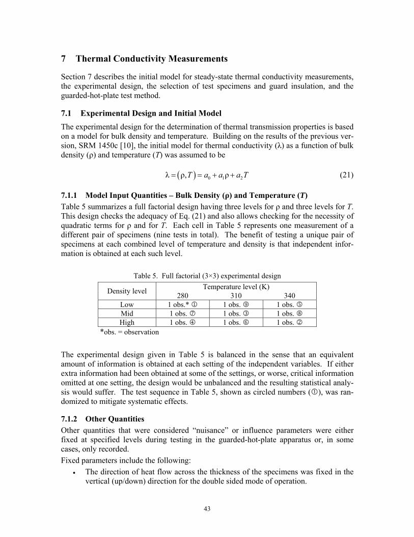
43

7 Thermal Conductivity Measurements

Section 7 describes the initial model for steady-state thermal conductivity measurements, the experimental design, the selection of test specimens and guard insulation, and the guarded-hot-plate test method.

7.1 Experimental Design and Initial Model The experimental design for the determination of thermal transmission properties is based on a model for bulk density and temperature. Building on the results of the previous ver-sion, SRM 1450c [10], the initial model for thermal conductivity (λ) as a function of bulk density (ρ) and temperature (T) was assumed to be

( ) 0 1 2λ ρ, ρT a a a T= = + + (21)

7.1.1 Model Input Quantities – Bulk Density (ρ) and Temperature (T) Table 5 summarizes a full factorial design having three levels for ρ and three levels for T. This design checks the adequacy of Eq. (21) and also allows checking for the necessity of quadratic terms for ρ and for T. Each cell in Table 5 represents one measurement of a different pair of specimens (nine tests in total). The benefit of testing a unique pair of specimens at each combined level of temperature and density is that independent infor-mation is obtained at each such level.

Table 5. Full factorial (3×3) experimental design

Temperature level (K) Density level 280 310 340 Low 1 obs.* 1 1 obs. 9 1 obs. 5 Mid 1 obs. 7 1 obs. 3 1 obs. 8 High 1 obs. 4 1 obs. 6 1 obs. 2

*obs. = observation

The experimental design given in Table 5 is balanced in the sense that an equivalent amount of information is obtained at each setting of the independent variables. If either extra information had been obtained at some of the settings, or worse, critical information omitted at one setting, the design would be unbalanced and the resulting statistical analy-sis would suffer. The test sequence in Table 5, shown as circled numbers ( ), was ran-domized to mitigate systematic effects.

7.1.2 Other Quantities Other quantities that were considered “nuisance” or influence parameters were either fixed at specified levels during testing in the guarded-hot-plate apparatus or, in some cases, only recorded. Fixed parameters include the following:

• The direction of heat flow across the thickness of the specimens was fixed in the vertical (up/down) direction for the double sided mode of operation.

44

• The temperature difference (ΔT) across the specimen was fixed at 25 K and fol-lowed standard practice for selecting test temperatures [17].

• The clamping pressure (f ) applied to the specimens was maintained at a nominal value of 490 kPa for all tests.

• The chamber air temperature (Ta) of the apparatus chamber was controlled to within 0.1 K, or less, of the mean specimen temperature (Tm).

Recorded parameters include the following: • The chamber air pressure (pa) was uncontrolled and varied with changes in the

barometric pressure. • The chamber relative humidity was, in general, maintained below 10 % RH by us-

ing a dry-air purge during the tests. The relative humidity, however, varied with the chamber dry-bulb air temperature (Ta).

7.2 Guarded-Hot-Plate Guard Insulation Table 6 summarizes the mass, dimensional, and bulk density measurements, rank ordered by bulk density for the 25 sheets of guard insulation prepared from the auxiliary material described earlier. The purpose of the auxiliary material was to function as radial guard

Table 6. Physical properties of guarded-hot-plate guard insulation

Index ID Mass (kg)

Area (m2)

Thickness (m)

Bulk density (kg·m-3)

1 22 1.29664 0.4365 0.02544 116.8 2 01 1.31080 0.4367 0.02538 118.3 3 07 1.32077 0.4378 0.02546 118.5 4 06 1.34583 0.4383 0.02590 118.6 5 02 1.34312 0.4380 0.02585 118.7 6 23 1.34539 0.4367 0.02596 118.7 7 08 1.34656 0.4378 0.02568 119.8 8 17 1.34565 0.4383 0.02557 120.1 9 12 1.35763 0.4402 0.02564 120.3

10 10 1.35535 0.4382 0.02563 120.7 11 20 1.34345 0.4363 0.02550 120.7 12 14 1.35243 0.4359 0.02565 120.9 13 09 1.34849 0.4390 0.02536 121.1 14 04 1.37192 0.4375 0.02585 121.3 15 16 1.37639 0.4373 0.02591 121.5 16 11 1.34186 0.4365 0.02530 121.5 17 18 1.38021 0.4367 0.02599 121.6 18 21 1.38539 0.4397 0.02584 121.9 19 19 1.37329 0.4388 0.02564 122.1 20 13 1.35383 0.4374 0.02535 122.1 21 05 1.35820 0.4380 0.02532 122.5 22 03 1.38218 0.4388 0.02565 122.8 23 15 1.36588 0.4373 0.02531 123.4 24 25 1.39927 0.4370 0.02589 123.7 25 24 1.39067 0.4352 0.02559 124.9

45

insulation for the panels during thermal testing in the guarded-hot-plate apparatus. The guards were prepared by cutting a 1016 mm diameter circular section from the center of each sheet and removing a center square (void) 610 mm by 610 mm. Supplementary mass and dimensional measurements were carried out to determine the bulk density for the guard insulation (Table 6).

7.3 Specimen Selection The 450 panels (Table 3) were rank ordered by bulk density and divided into 25 subsets of 18 panels. The average bulk density was computed for each of the 25 subsets of 18 panels and cross-matched, as closely as possible, with the corresponding guard insulation bulk density in Table 6. The cross-matching process retained the same number of density levels given in Table 5 (low, mid, and high) resulting in a final selection of 18 (nine pairs of) panels and their corresponding guard insulation. The specimens for guarded-hot-plate testing were assembled by placing an insulation panel in the equivalent sized void in the center of the corresponding guard insulation. Table 7 summarizes the bulk densities for the nine specimen pairs and guard insulation.

Table 7. Test specimens for (3×3) experimental design

ID Bulk density (kg·m-3) Density level

Specimen pair Panel Guard Panel Guard

182 22 112.2 116.8 Low 1 437 01 114.2 118.3 049 07 115.0 118.5 Low 2 086 06 115.6 118.6 397 02 116.1 118.7 Low 3 266 23 116.4 118.7 257 12 117.9 120.3 Mid 4 137 10 118.2 120.7 184 20 118.5 120.8 Mid 5 369 14 118.8 120.9 339 09 119.1 121.1 Mid 6 355 04 119.5 121.3 345 18 120.7 121.6 High 7 030 21 121.0 121.9 028 13 121.9 122.1 High 8 118 05 122.5 122.5 009 25 123.3 123.7 High 9 192 24 125.0 124.9

7.4 Thermal Conductivity Apparatus

7.4.1 Guarded-Hot-Plate Method The thermal conductivity measurements were determined using the NIST 1016 mm guarded-hot-plate apparatus operated in the double sided mode. Figure 12 shows the essential features of the guarded-hot-plate apparatus designed for operation near ambient temperature con-

46

ditions. The apparatus is cylindrically symmetric about the axis indicated in Fig. 12. The plates are horizontal and heat flow (Q) is vertical (up/down) through the pair of specimens. The specimens, which have nearly the same density, size, and thickness, are placed on each surface of the guarded hot plate and clamped securely by the cold plates. The guarded hot plate and the cold plates provide constant-temperature boundary conditions to the specimen surfaces. With proper guarding, lateral heat flows (Qg and Qe) are reduced to negligible proportions and, under steady-state conditions, the apparatus provides one-dimensional heat flow (Q) normal to the meter area of the specimen pair. A secondary guard is provided by an enclosed chamber that conditions the ambient air surrounding the plates to a temperature near to the mean speci-men temperature (i.e., average surface temperatures of the hot and cold plates in contact with the specimens).

Equation (22) is the operational definition [18] for the experimental thermal conductivity6 of the specimen pair (λexp)

exp1 2

λ[( / ) ( / ) ]

QA T L T L

=Δ + Δ

(22)

6 The thermal transmission properties of heat insulators determined from standard test methods typically include several mechanisms of heat transfer, including conduction, radiation, and possibly convection. For that reason, some experimentalists will include the adjective “apparent” when describing thermal conduc-tivity of thermal insulation. However, for brevity, the term thermal conductivity is used in this report.

Figure 12. Guarded-hot-plate schematic, double-sided mode of operation – vertical heat flow.

1. Principle: Tc < Th; Tc1 = Tc2 = Tc2. Practice: Tc < Th; Tc1 ≈ Tc2 ≈ Tc

Guarded hot plate (Meter plate)

Guard plate

Ambient gas Cold plate 2

Qg Qe

Qe Qe

Qe

Cold plate 1

Qg

Specimen 2

Specimen 1

Tc1

Tc2

Th

Q 2

Q 2

F1

F2

47

where Q and A are defined in Terminology and (ΔT /L)1 is equal to the ratio of the surface-to-surface temperature difference (Th – Tc) to the thickness (L) for Specimen 1. A similar expression is used for Specimen 2.

When the temperature differences and the specimen thicknesses are nearly the same, re-spectively, Eq. (22) reduces to

expλ2

avg

avg

QLA T

=Δ

(23)

In the double-sided mode of operation, the thermal transmission properties correspond to a mean temperature Tm given by Tm = (Th + Tc)/2.

7.4.2 1016 mm Guarded-Hot-Plate Apparatus The NIST 1016 mm guarded-hot-plate apparatus and uncertainty assessment, under operat-ing conditions near room conditions, have been described previously [16]. The apparatus plates, 1016 mm in diameter, were fabricated from 6061-T6 aluminum alloy and the surfaces in contact with the specimens were anodized black to have an emittance (ε) of 0.89. The me-ter plate is nominally 406 mm in diameter and is physically separated from the surrounding guard plate by an air gap (Fig. 12).

7.5 Establishing and Demonstrating Traceability Section 7.5 describes the metrological traceability for measurement results for the NIST 1016 mm guarded-hot-plate apparatus. Table 8 summarizes the calibration information for the input quantities for Eq. (2) and the influence quantities described in Sec. 7.1.2. The quan-tities are ultimately traceable to reference standards retained by other organizations at NIST which maintain practical realizations of the base SI units. The expanded uncertainties in Ta-ble 8 are used as part of the uncertainty analysis described in Sec. 7.6 and Sec. 8.4.

Table 8. Calibration information for the NIST 1016 mm guarded-hot-plate apparatus

Quantity

Calibration laboratory Expanded

uncertainty (k = 2)

Interval Rs NIST Quantum Electrical Metrology Division 0.000 000 5 Ω 1 year

Vm, Vs Manufacturer of digital multimeter 0.029 %* 2 year Th, Tc NIST Thermometry Group < 0.005 °C 10 year

L NIST Engineering Metrology Group < 70 nm 10 year ro, ri Internal check – pin gages 0.01 mm α Handbook data (Standard Reference Data) 20 % N.A. F NIST Mass and Force Group 0.001 % 2 year ε Internal check – infrared reflectometer 4 % Ta Internal check – thermistor probe 0.4 °C 5 year pa NIST Pressure and Vacuum Group 52 Pa 5 year

RH Manufacturer of relative humidity instrument 1 % 5 year *30 mV range

48

The first six rows of Table 8 represent the input quantities for the determination of λ from Eq. (2). The last five rows are influence quantities that can affect the determination of λ dur-ing a test and are either fixed at a particular level or are generally neglected due to the small effect and limited (“floating”) range. Sections 7.5.1 through 7.5.5 describe, in detail, the calibration information given in Table 8.

7.5.1 Specimen Heat Flow - Q The specimen heat flow Q is essentially determined by measuring the direct current and voltage provided to the meter-plate heater (Qm). The measurement approach for Qm is shown schematically in Fig. 13. A direct-current (DC) power supply provides current (I) to the circuit which is determined by the measurement Vs across the four-terminal 0.1 Ω stan-dard resistor placed in an oil bath at 25.00 °C.

The equation for the determination of Qm is

sm m m

s

VQ I V VR

= = (24)

where I is the current (Vs /Rs) measured at the standard resistor and Vm is the voltage drop in the meter-plate heater measured across voltage taps located at the midpoint of the gap be-tween the meter plate and guard plate.

7.5.1.1 Standard Resistor Calibration The standard resistor (Fig. 13) is a commercial, double-walled manganin resistor [19] manu-factured in 1913. For 33 years, the resistor has been calibrated by the NIST Quantum Elec-trical Metrology Division in a mineral oil bath at 25 °C. Since 1990, the NIST calibrations have been based on the quantum Hall effect used as the U.S. representation of the ohm [20-21]. The 2010 calibration (at a test current of 0.316 A) assigned a value of 0.10006939 Ω ± 0.000 000 5 Ω (expanded uncertainty, k = 2) to the resistor.

Figure 13. Electrical schematic for meter-plate power measurement.

DC Power Supply

0.1 Ω Standard

Resistor, Rs

56 Ω Meter-plate Heater, Rm

I

Vs VmOil Bath 25.00 °C

49

7.5.1.2 Digital Multimeter Calibration A digital multimeter (DMM), which is part of an automated computer data acquisition sys-tem, is used for the DC voltage measurement of Vs and Vm. At 2 year intervals (Table 8), the DMM and data acquisition unit are removed from laboratory service and calibrated by the manufacturer to their specifications, typically at an offsite location. The measurement results supporting the calibration are traceable to NIST. After return, the DMM and data acquisition unit are placed in service and performance checks of the hardware are con-ducted manually and with computer software.

7.5.2 Temperature Difference - ΔT The temperature difference across the specimen is determined by small capsule industrial plati-num resistance thermometers (PRTs) located in the hot and cold plates (Th and Tc, respec-tively). Each thermometer is constructed of a strain- free platinum element supported in a gold-plated copper cylinder 3.18 mm in diameter by 9.7 mm long backfilled with helium gas and hermetically sealed. The operational range is from –260 °C to 260 °C and the nominal electri-cal resistance is 100 Ω at 0 °C. The electrical resistance of each 4-wire PRT is measured with the DMM and automated data acquisition system described in Sec. 7.5.1.2.

For 29 years, the PRTs have been calibrated by the NIST Thermometry Group by compari-son with a standard platinum resistance thermometer (SPRT) in a stirred liquid calibration bath [22]. The PRTs were initially calibrated in 1981 at the triple point of water (which is 0.01 °C by definition), 10 °C, 20 °C, 30 °C, 40 °C, and 50 °C. In 1993, the PRTs were re-moved from the apparatus and calibrated over an extended temperature range, thereby ex-tending the range of the guarded-hot-plate apparatus. All temperatures for the 1993 and 2008 calibrations were based on the International Temperature Scale of 1990 (ITS-90) [23-24]. For the 2008 calibration, the expanded uncertainty (k = 2) in the bath temperature meas-urements from –70 °C to 0 °C did not exceed 0.0023 °C, from 0 °C to 95 °C did not exceed 0.0024 °C, and from 95 °C to 300 °C did not exceed 0.0048 °C.

7.5.3 Specimen Thickness - L For semi-rigid specimens such as SRM 1450d, the specimen thickness (L) is measured in-situ using eight (four for the top specimen and 4 for the bottom specimen) linear position transducers located at the periphery of the plate. The calibration hierarchy for these trans-ducer measurements is described in Sec. 7.5.3.1 and Sec. 7.5.3.2.

7.5.3.1 Fused-Quartz Spacers One set of nominal 25.4 mm spacers was cut and ground, collectively, by the NIST Glass Fabrication Shop from quartz tubing (25 mm outer diameter). Fused-quartz tubing was se-lected because of its low thermal expansion coefficient (5.5×10-7 K-1) and high elastic modulus (72 GPa). The set of spacers was measured using either a digital caliper or a digi-tal height gage referenced to a datum surface.

7.5.3.2 Linear Position Transducers For 1450d, the in-situ thickness of the specimen is determined by averaging four linear po-sition transducers attached to the periphery of each cold plate at approximate 90° arc inter-vals. Each positioning system consists of a digital readout and a slider translating on a tape

50

scale bonded to a precision ground plate of a low thermal expansion iron-nickel (FeNi36) alloy. The electrical windings on the scale are inductively coupled with the slider and the resulting output signal from the scale is resolved by the digital readout. The digital read-outs are reset by placing one set of fused-quartz spacers of known thickness between the cold plate and hot plate.

7.5.4 Meter Area - A The meter area is the mathematical area through which the heat input to the meter plate Qm flows normal to the heat-flow direction under ideal guarding conditions (i.e., lateral heat flows ≡ 0) into the specimen. The circular meter area was calculated from Eq. (25).

( ) ( )2 2 2π 1 α2 o i mpA r r T= × + × + Δ (25)

where ro is the outer radius of the meter plate (m); ri is the inner radius of the guard plate (m); α is the coefficient of thermal expansion of 6061-T6 aluminum (K-1); and, ΔTmp is the temperature of the meter plate (Th) minus 20 °C (in kelvin).

7.5.4.1 Plate Dimensions The design dimensions for the meter plate and the guard plate diameters are 405.64 mm and 407.42 mm, respectively. A coordinate measuring machine (CMM) measured the roundness of the meter plate at six locations at the periphery and the diameter was determined to be 405.67 mm (within 0.03 mm of the design dimension). A uniform gap width of 0.89 mm was established using three precision pin gages spaced between the meter plate and guard plate at equiangular intervals. The uncertainty of the pin gages was +0.005 mm/–0.000 mm. Based on these check measurements, the input values for ro and ri for Eq. (25) were deter-mined to be 0.20282 m and 0.20371 m, respectively, and the standard uncertainty (k = 1) for both input values was taken to be 0.0254 mm.

7.5.4.2 Thermal Expansion Effects For α, an input value of 23.6×10-6 K-1 at 20 °C was obtained from aggregated handbook data [25] for 6061-T6 aluminum. The standard uncertainty (k = 1) for the value of α was estimated conservatively to be 10 % (2.36×10-6 K-1). The standard uncertainty (k = 1) for ΔTmp was based the uncertainty for the plate temperature (Sec. A4.3.3).

7.5.5 Influence (Secondary) Quantities Several other quantities can affect the thermal conductivity measurement of insulating ma-terials including the clamping load, plate emittance, chamber air temperature, pressure, and relative humidity, among others. These quantities are either controlled at a fixed value dur-ing a test or recorded. The quantities were not included in the uncertainty analysis.

7.5.5.1 Plate Parameters The clamping load (F) for each cold plate is measured by a 4.4 kN load cell connected to a dual-channel digital readout. The load cells and readout were removed from the apparatus and calibrated, as a system, by the NIST Mass and Force Group by application of dead

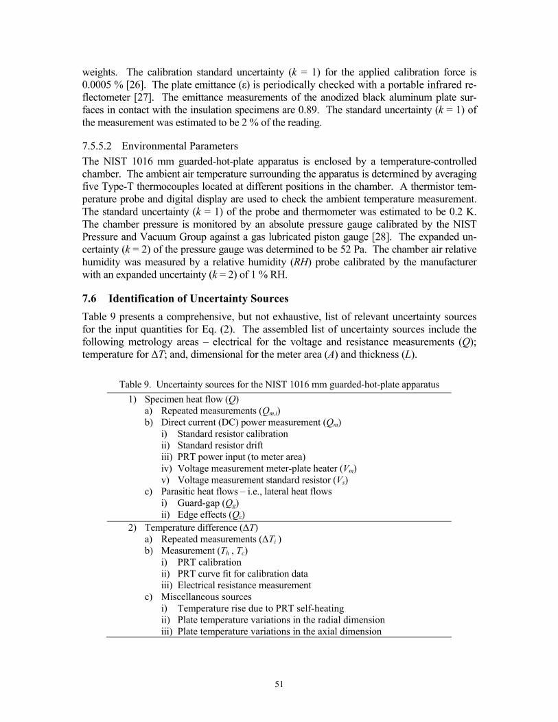
51

weights. The calibration standard uncertainty (k = 1) for the applied calibration force is 0.0005 % [26]. The plate emittance (ε) is periodically checked with a portable infrared re-flectometer [27]. The emittance measurements of the anodized black aluminum plate sur-faces in contact with the insulation specimens are 0.89. The standard uncertainty (k = 1) of the measurement was estimated to be 2 % of the reading.

7.5.5.2 Environmental Parameters The NIST 1016 mm guarded-hot-plate apparatus is enclosed by a temperature-controlled chamber. The ambient air temperature surrounding the apparatus is determined by averaging five Type-T thermocouples located at different positions in the chamber. A thermistor tem-perature probe and digital display are used to check the ambient temperature measurement. The standard uncertainty (k = 1) of the probe and thermometer was estimated to be 0.2 K. The chamber pressure is monitored by an absolute pressure gauge calibrated by the NIST Pressure and Vacuum Group against a gas lubricated piston gauge [28]. The expanded un-certainty (k = 2) of the pressure gauge was determined to be 52 Pa. The chamber air relative humidity was measured by a relative humidity (RH) probe calibrated by the manufacturer with an expanded uncertainty (k = 2) of 1 % RH.

7.6 Identification of Uncertainty Sources Table 9 presents a comprehensive, but not exhaustive, list of relevant uncertainty sources for the input quantities for Eq. (2). The assembled list of uncertainty sources include the following metrology areas – electrical for the voltage and resistance measurements (Q); temperature for ΔT; and, dimensional for the meter area (A) and thickness (L).

Table 9. Uncertainty sources for the NIST 1016 mm guarded-hot-plate apparatus

1) Specimen heat flow (Q) a) Repeated measurements (Qm,i) b) Direct current (DC) power measurement (Qm)

i) Standard resistor calibration ii) Standard resistor drift iii) PRT power input (to meter area) iv) Voltage measurement meter-plate heater (Vm) v) Voltage measurement standard resistor (Vs)

c) Parasitic heat flows – i.e., lateral heat flows i) Guard-gap (Qg) ii) Edge effects (Qε) iii)

2) Temperature difference (ΔT) a) Repeated measurements (ΔTi ) b) Measurement (Th , Tc)

i) PRT calibration ii) PRT curve fit for calibration data iii) Electrical resistance measurement

c) Miscellaneous sources i) Temperature rise due to PRT self-heating ii) Plate temperature variations in the radial dimension iii) Plate temperature variations in the axial dimension

52

3) Thickness (L) a) Multiple measurement locations b) Instrument (in-situ) measurement (i.e., linear position system)

i) Gage block calibration ii) Fused-quartz spacer length dimensions

(1) Multiple locations (2) Micrometer uncertainty

iii) System uncertainty iv) Short-term repeatability

c) Plate characteristics i) Flatness

(1) Multiple locations (2) Coordinate measuring machine (CMM) uncertainty

ii) Deflection under axial loading of cold plates iii)

4) Meter area (A) a) Plate dimensions b) Thermal expansion effects c) Temperature measurement

53

8 Data and Uncertainty Evaluation

Section 8 presents the thermal conductivity measurements, analysis of data, final model determination, and assessment of measurement uncertainties.

8.1 Experimental Design Modification The thermal conductivity measurements were initially completed using the experimental design shown in Table 5. Least squares fits of multiple models of the thermal conductiv-ity data revealed that, for the densities studied, λexp was insensitive to bulk density (ρ). In other words, λexp was found to be a function only of temperature (T). To confirm this finding, the experimental design was modified by adding two intermediate temperature levels at 295 K and 325 K. The resulting full factorial design with three levels for density and five levels of temperature is shown in Table 10. The corresponding test sequence in Table 10, from 10 to 15 (shown as circled numbers), was randomized to mitigate the in-fluence of any systematic effects.

Table 10. Full factorial (3×5) experimental design

Temperature level (K) Density level 280 295 310 325 340 Low 1 obs.* 1 obs. 1 obs. 1 obs. 1 obs. Mid 1 obs. 1 obs. 1 obs. 1 obs. 1 obs. High 1 obs. 1 obs. 1 obs. 1 obs. 1 obs.

*obs. = observation

An additional 12 test specimens (six pairs) were selected from the material lot to augment the original 18 specimens selected in Table 7. Table 11 summarizes the selection for the six additional specimen pairs and corresponding guard insulation. Some insulation guards were re-used for these subsequent tests.

Table 11 – Additional test specimens for (3×5) experimental design

ID Bulk density (kg·m-3) Density level

Specimen pair Panel Guard Panel Guard

103 01 113.5 118.3 Low 10 332 07 114.9 118.5 308 06 115.4 118.6 Low 11 164 02 115.8 118.7 074 10 118.1 120.7 Mid 12 087 20 118.5 120.7 107 14 118.9 120.9 Mid 13 155 09 118.9 121.1 105 05 121.3 122.5 High 14 347 03 121.7 122.8 129 15 122.9 123.7 High 15 351 25 123.7 124.9

1

2

3

4

5

6

7 8

9

10

11

12 13

14

15

54

8.2 Guarded-Hot-Plate Data

8.2.1 Data Acquisition Thermal test data (Th, Tc, and Q) were collected every 2 min during a 4 h steady-state pe-riod (n = 120 observations per parameter) using a computer-controlled data acquisition system. The variability (s) for each measured parameter was checked against the accept-able tolerance limits summarized in Table 12. Estimates for each measured parameter were (subsequently) taken as the arithmetic means of the observations.

Table 12. Required tolerance limits for acceptable steady-state test data

Quantity Description Limits Units Th Hot surface ±0.0025 K Tc Cold surface ±0.005 K ΔT Temperature difference ±0.005 K Q Meter-area heat flow ±0.01 W Vg Thermopile voltage ±0.7 μV Ta Chamber air temperature ±0.05 K RH Chamber relative humidity maintained < 10 % RH pa Chamber air pressure uncontrolled kPa

8.2.2 Data Summary (Tabular Format) Table 13 summarizes the experimental results – specimen information, input estimates, influencing factor estimates, and the output estimate for measured thermal conductivity (λexp) – for the 15 specimen pairs specified in the experimental design (Table 10). The rows of data in Table 13 are grouped by Tm from 280 K to 340 K and, within each level of Tm, the average specimen densities (ρs) are arranged from lowest to highest value. The columns of data are grouped into four major sections: 1) specimen identification (ID) and material properties; 2) input quantities for Eq. (23); 3) secondary quantities; and 4) resultant thermal conductivity (λ).

The notations “1” and “2” in Table 13 designate the top and bottom specimen, respec-tively, as illustrated in Fig. 12. The bulk density parameter ρs (Table 13, column 6) is the average of ρ1 and ρ2. The range for ρs defines the “certified” bulk density range for SRM 1450d from 113.5 kg·m-3 to 123.8 kg·m-3 (rounded7 from 114 kg·m-3 to 124 kg·m-3). The input temperature estimates, Th, Tc1, and Tc2, were within 0.01 K, or less, of their respec-tive set-point temperatures. The estimates of Q/2 ranged from 3.9 W to 4.8 W for Tm at 280 K and 340 K, respectively. For a fixed value of Tm, the variation of Q/2 due to changes in ρs was much smaller. The estimates for A have been corrected for thermal ex-pansion effects of the meter-plate radius using Eq. (25). The estimates for the in-situ test thickness L were determined by averaging the digital outputs of the eight linear position transducers (four for each cold plate) discussed in Sec. 7.5.3. The resultant estimates for λexp include an extra digit to reduce rounding errors. 7 The panel bulk densities (ρ1 and ρ2) given in Table 13 were determined using the in-situ test thicknesses (L). Consequently, the values for ρ1 and ρ2 are slightly different (by 0.5 %, or less) than the values given in Ta-ble 3, which were determined using the mean thickness (Lm) of the surface plate measurements (Figure 3a).

55

Ta

ble

13 –

The

rmal

con

duct

ivity

dat

a (s

orte

d by

Tm a

nd ρ

s)

Spec

imen

pro

perti

es

Inpu

t qua

ntiti

es fo

r Eq.

(22)

Se

cond

ary

quan

titie

s

T m

ID 1

ID

2

ρ 1

ρ 2

ρ s

T h

T c1

T c2

Q/2

A

L T a

p a

RH

f

λ exp

* (K

)

(k

g·m

-3)

(kg·

m-3

) (k

g·m

-3)

(K)

(K)

(K)

(W)

(m2 )

(mm

) (K

) (k

Pa)

(%)

(Pa)

(W

·m-1

·K-1

) 28

0 18

2 43

7 11

2.8

114.

3 11

3.5

292.

50

267.

50

267.

50

3.89

5 0.

1298

0 25

.93

280.

0 99

.3

8 47

7 0.

0311

2 28

0 25

7 13

7 11

8.3

118.

7 11

8.5

292.

50

267.

50

267.

51

3.89

4 0.

1298

0 25

.80

280.

0 99

.6

8 45

7 0.

0309

6 28

0 34

5 03

0 12

1.0

121.

4 12

1.2

292.

50

267.

50

267.

49

3.92

4 0.

1298

0 25

.56

280.

0 10

0.6

9 47

8 0.

0309

0 29

5 10

3 33

2 11

3.5

115.

2 11

4.3

307.

50

282.

50

282.

50

4.05

0 0.

1298

9 26

.02

295.

0 10

0.5

4 46

0 0.

0324

5 29

5 07

4 08

7 11

8.9

119.

1 11

9.0

307.

50

282.

50

282.

50

4.08

6 0.

1298

9 25

.82

295.

0 10

0.6

4 46

1 0.

0324

9 29

5 10

5 34

7 12

1.1

121.

8 12

1.5

307.

50

282.

50

282.

50

4.10

5 0.

1298

9 25

.80

295.

0 10

0.2

3 47

2 0.

0326

1 31

0 04

9 08

6 11

6.0

115.

6 11

5.8

322.

50

297.

50

297.

50

4.24

0 0.

1299

8 26

.13

310.

0 10

0.1

2 48

4 0.

0340

9 31

0 18

4 36

9 11

8.5

118.

9 11

8.7

322.

50

297.

50

297.

50

4.32

4 0.

1299

8 25

.76

310.

0 98

.6

2 50

6 0.

0342

8 31

0 02

8 11

8 12

2.0

122.

8 12

2.4

322.

50

297.

51

297.

50

4.31

7 0.

1299

8 25

.76

310.

0 99

.7

2 48

8 0.

0342

2 32

5 30

8 16

4 11

5.2

116.

1 11

5.7

337.

50

312.

50

312.

50

4.49

4 0.

1300

7 25

.85

325.

0 10

0.5

1 49

5 0.

0357

2 32

5 10

7 15

5 11

8.8

118.

9 11

8.9

337.

50

312.

50

312.

50

4.49

9 0.

1300

7 26

.00

325.

0 10

1.3

1 49

1 0.

0359

7 32

5 12

9 35

1 12

2.5

123.

9 12

3.2

337.

50

312.

50

312.

50

4.54

9 0.

1300

7 25

.73

325.

0 97

.5

1 50

1 0.

0359

9 34

0 39

7 26

6 11

5.3

116.

4 11

5.8

352.

50

327.

49

327.

50

4.70

1 0.

1301

6 25

.98

340.

0 99

.7

1 46

6 0.

0375

2 34

0 33

9 35

5 11

8.6

119.

7 11

9.1

352.

50

327.

50

327.

50

4.74

7 0.

1301

6 25

.78

340.

0 10

1.3

1 47

8 0.

0376

0 34

0 00

9 19

2 12

3.3

124.

3 12

3.8

352.

50

327.

50

327.

49

4.76

0 0.

1301

6 25

.85

340.

0 99

.1

<1

432

0.03

782

* Ex

tra d

igit

incl

uded

for r

ound

ing

56

During a test, the (secondary) influence quantities (Ta, pa, RH, and f ) were either con-trolled or only recorded. The chamber air temperature (Ta) was controlled to be the same temperature as Tm (within 0.1 K, or less). The chamber air pressure (pa) varied with the site barometric conditions from 97.5 kPa to 101.3 kPa. The chamber RH was maintained at less than 10 % RH by a dry-air purge. However, the value varied with the chamber dry-bulb air temperature (Ta). The clamping pressure (f ) was determined by averaging the loading force (F) applied by each cold plate divided by the surface area of the cold plate, which was corrected for thermal expansion effects.

Table 14 provides summary statistics for test quantities given in Table 13 that were fixed at one value across all tests. As noted in Sec.7.1.2, the temperature difference (ΔT) of 25.001 K was based on standard practice for selecting test temperatures [17].

Table 14. Summary statistics for fixed- and recorded-value quantities

ΔT (K)

L (mm)

pa (kPa)

f (Pa)

Mean 25.001 25.85 99.9 476 Std. Dev. 0.003 0.14 1.0 19

Prior to testing, each specimen pair was assembled with its respective guard insulation and was placed in an oven at 100 °C for a minimum of 3 h. The panels and guard insula-tion assemblies were weighed prior to, and after, the guarded-hot-plate tests. The average mass regain for the specimen assemblies was approximately 8 g (or 0.3 %).

8.2.3 Data Screening (Graphical Analysis) Figures 14a and 14b plot values of λexp from Table 13 as a function of the design model (Eq. (21)) input variables ρs and Tm, respectively. For Fig. 14a, the individual data points are plotted as filled circle symbols corresponding to Tm levels of 280 K, 295 K, 310 K, 325 K, and 340 K. The error bars represent expanded uncertainties of 0.86 % (Sec. 8.4.1). For Fig. 14b, the individual data points are plotted as filled circle, square, and triangle sym-bols (without error bars for clarity) corresponding to the three main levels selected for bulk density.

8.2.4 Data Evaluation – Characterization The data in Fig. 14 strongly suggest that, in the range of ρs and Tm covered for the 450 specimens comprising the current SRM:

1) λexp is insensitive to ρs (in contrast with previous 1450 version materials); and, 2) the dependence of λexp on Tm is strongly linear.

The first assertion is born out by linear least squares fits to the 3-point horizontal profiles visible in Fig. 14a. Table 15 summarizes the slopes of the lines shown in Fig. 14a and their corresponding t-values. For the three inner horizontal profiles, the slope of the fitted profile is statistically indistinguishable from zero (|t| ≤ 2) at 95% confidence for the 310 K and 325 K lines and only marginally significant (|t| = 2) for the 295 K line. For the two outer horizontal profiles (280 K and 340 K), the slopes are statistically significant, but quite small.

57

270 280 290 300 310 320 330 340 350

0.030

0.031

0.032

0.033

0.034

0.035

0.036

0.037

0.038

0.039

Temperature, K

Ther

mal

con

duct

ivity

, W· m

-1· K

-1

Low Bulk DensityMid Bulk DensityHigh Bulk Density

110 115 120 1250.030

0.031

0.032

0.033

0.034

0.035

0.036

0.037

0.038

0.039

Bulk density, kg·m-3

280 K

295 K

310 K

325 K

340 K

a)

b)

Ther

mal

con

duct

ivity

, W· m

-1· K

-1

Figure 14. 1450d: a) Graphical analysis of thermal conductivity versus bulk density. Error bars represent ex-panded uncertainties of 0.86 %. b) Graphical analysis of thermal conductivity (without error bars for clarity) versus temperature.

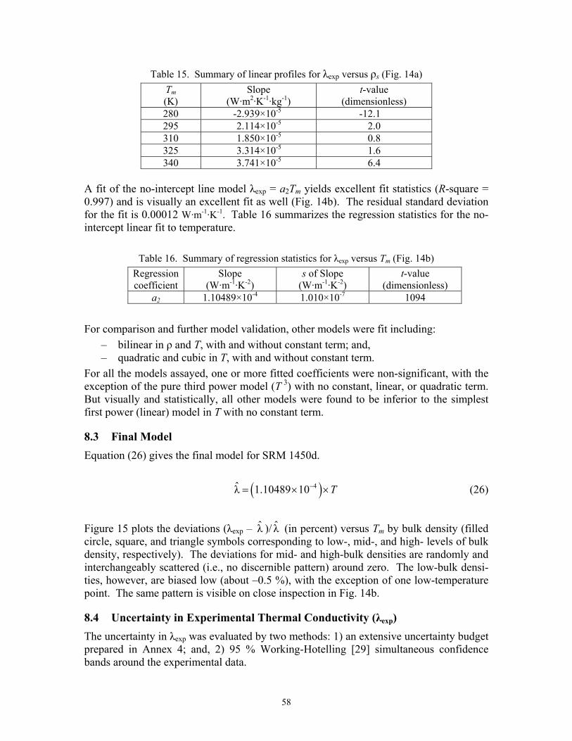
58

Table 15. Summary of linear profiles for λexp versus ρs (Fig. 14a) Tm (K)

Slope (W·m2·K-1·kg-1)

t-value (dimensionless)

280 -2.939×10-5 -12.1 295 2.114×10-5 2.0 310 1.850×10-5 0.8 325 3.314×10-5 1.6 340 3.741×10-5 6.4

A fit of the no-intercept line model λexp = a2Tm yields excellent fit statistics (R-square = 0.997) and is visually an excellent fit as well (Fig. 14b). The residual standard deviation for the fit is 0.00012 W·m-1·K-1. Table 16 summarizes the regression statistics for the no-intercept linear fit to temperature.

Table 16. Summary of regression statistics for λexp versus Tm (Fig. 14b)

Regression coefficient

Slope (W·m-1·K-2)

s of Slope (W·m-1·K-2)

t-value (dimensionless)

a2 1.10489×10-4 1.010×10-7 1094

For comparison and further model validation, other models were fit including: – bilinear in ρ and T, with and without constant term; and, – quadratic and cubic in T, with and without constant term.

For all the models assayed, one or more fitted coefficients were non-significant, with the exception of the pure third power model (T 3) with no constant, linear, or quadratic term. But visually and statistically, all other models were found to be inferior to the simplest first power (linear) model in T with no constant term.

8.3 Final Model Equation (26) gives the final model for SRM 1450d.

( )4λ 1.10489 10 T−= × × (26)

Figure 15 plots the deviations (λexp – λ )/ λ (in percent) versus Tm by bulk density (filled circle, square, and triangle symbols corresponding to low-, mid-, and high- levels of bulk density, respectively). The deviations for mid- and high-bulk densities are randomly and interchangeably scattered (i.e., no discernible pattern) around zero. The low-bulk densi-ties, however, are biased low (about –0.5 %), with the exception of one low-temperature point. The same pattern is visible on close inspection in Fig. 14b.

8.4 Uncertainty in Experimental Thermal Conductivity (λexp) The uncertainty in λexp was evaluated by two methods: 1) an extensive uncertainty budget prepared in Annex 4; and, 2) 95 % Working-Hotelling [29] simultaneous confidence bands around the experimental data.

59

270 280 290 300 310 320 330 340 350-1.0

-0.5

0.0

0.5

1.0

Temperature, K

Dev

iatio

ns,

%

Low Bulk DensityMid Bulk DensityHigh Bulk Density

Figure 15. 1450d: Graphical analysis of deviations (in %) for the fit given in Eq. (26).

8.4.1 Uncertainty Budget For the multiplicative expression of Eq. (23), the relative combined standard uncertainty in λexp can be expressed as the relative uncertainties associated with each factor combined in quadrature.

( ) ( ) ( ) ( ) ( ) ( )2 2 2 2exp

, expexp

λλ

λc

c rel

u u Q u T u L u Au

Q T L A⎛ ⎞ ⎛ ⎞ ⎛ ⎞ ⎛ ⎞Δ

= = + + +⎜ ⎟ ⎜ ⎟ ⎜ ⎟ ⎜ ⎟Δ⎝ ⎠ ⎝ ⎠ ⎝ ⎠ ⎝ ⎠ (27)

The standard uncertainties and input quantities used in Eq. (27) are derived in Annex 4. The maximum combined standard uncertainty for λexp was determined at Tm of 340 K.

( )2 2 2 2

, exp0.0074 0.077 0.065 0.000043λ4.736 25.001 25.85 0.13016c relu ⎛ ⎞ ⎛ ⎞ ⎛ ⎞ ⎛ ⎞= + + +⎜ ⎟ ⎜ ⎟ ⎜ ⎟ ⎜ ⎟

⎝ ⎠ ⎝ ⎠ ⎝ ⎠ ⎝ ⎠ (28)

( ) ( ) ( ) ( ) ( )2 2 2 2, expλ 0.00156 0.00308 0.00251 0.00033 0.0043c relu = + + + = (29)

( ) ( )exp , expλ 2 λ 0.0086rel c relU u= = (30)

60

Expressed as a percent (× 100), Urel is equal to 0.86 %.

The relative contribution for the first term in Eq. (29) is 13.3 %; for the second, 51.9 %; for the third, 34.2 %; and, for the fourth, 0.6 %. The major contributory uncertainties for SRM 1450d are due to the empirical determinations for specimen temperature difference (ΔT) and thickness (Lavg). These findings are consistent with results from previous uncer-tainty analyses [16].

8.4.2 Confidence Limits (Working-Hotelling Bands) Figure 16 shows simultaneous 95 % confidence bands (dashed lines) about the no-intercept linear regression of λexp on T. The bands are actually hyperbolic segments, more constricted towards the middle of the temperature range, flaring out towards the ex-tremes of the range, where the least squares predictions are less certain. The “simultane-ous” refers to the fact that for any fixed value of T, a bona fide 95 % interval for thermal conductivity can be derived from the picture by drawing a vertical line segment at that value of T intersecting the lower band, fitted line, and upper band. The lower and upper band ordinate values thus determined form a 95 % confidence interval for the true value of λ at that T. The uncertainty from this approach is derived from the vertical segments at the ends of the temperature range (280 K or 340 K). Rounded up slightly, it is ±0.5 %.

270 280 290 300 310 320 330 340 350

0.030

0.031

0.032

0.033

0.034

0.035

0.036

0.037

0.038

0.039

Temperature, K

Ther

mal

con

duct

ivity

, W·m

-1·K

-1

Low Bulk DensityMid Bulk DensityHigh Bulk Density

Figure 16. 1450d: 95 % Confidence Limits (Working-Hotelling Bands [29]) about the no-intercept linear regression line λexp on T.

61

8.4.3 Comments on Uncertainty Approach The extensive uncertainty budget presented in Annex 4 has been developed over thirty years [30, 10, 16] and has been updated consistent with current international guidelines [15]. The budget uncertainty for this work was determined to be 0.86 % (k =2) which is a more conservative estimate than the maximum value based on the Working-Hotelling 95 % confidence bands of 0.5 % for the experimental data. For convenience to the SRM user, the uncertainty for 1450d has been rounded up to the nearest whole integer of 1 %.

8.4.4 Supplemental Thermal Conductivity Data As part of the imbalance experiment, specimen pair 184-369 was re-measured from 280 K to 340 K. The test results and analysis are presented in Annex 5.

62

9 Certification

Section 9 presents important summary information on the properties of interest, values and uncertainty, statement of metrology traceability, and instructions for use for Standard Reference Material 1450d. This information is intended to provide supplementary docu-mentation for the 1450d Certificate.

9.1 Properties of Interest Standard Reference Material 1450d is a high-density molded fibrous glass board certified for bulk density, ρ, and thermal conductivity, λ. Each SRM unit consists of a square panel of fine-glass fibers and phenolic binder molded into a semi-rigid board. The nomi-nal dimensions of a unit are 611 mm by 611 mm by 26 mm (Table 4) and the bulk den-sity ranges from 114 kg⋅m-3 to 124 kg⋅m-3 (Table 13).

9.2 Values and Uncertainties Each unit of SRM 1450d is individually certified for bulk density, ρ (Table 3), and batch certified for thermal conductivity with Eq. (31):

( )4λ 1.10489 10 mT−= × × (31)

where λ is the predicted thermal conductivity (W·m-1·K-1) and Tm is the mean specimen temperature (K). The test temperature difference across the specimen (ΔT) was 25 K (Table 14). Equation (31) is only certified to be valid over the temperature range of 280 K to 340 K. The expanded uncertainty for λ values from Eq. (31) is 1 % with a cov-erage factor of approximately k = 2.

9.3 Statement of Metrological Traceability The input quantities for the determination of bulk density and thermal conductivity are metrologically traceable to working references maintained at NIST as described in Sec. 6.4 and Sec. 7.5, respectively.

9.4 Instructions for Use Standard Reference Material 1450d is intended for use as a proven check for the guarded-hot-plate apparatus (or other absolute thermal conductivity apparatus) and for calibration of a heat-flow-meter apparatus over the temperature range of 280 K to 340 K. NIST can-not exclude the use of SRM 1450d for other purposes, but the user is cautioned that other purposes are not sanctioned by the 1450d Certificate.

9.4.1 Storage For protection and identification, it is recommended that the reference material be stored in the original packaging in a clean, dry environment at temperatures between 15 °C and 30 °C.

63

9.4.2 Preparation and Conditioning Before Measurement Prior to the thermal conductivity measurement, the reference material should be condi-tioned in laboratory conditions of 20 ° C to 25 °C and from 40 % RH to 65 % RH until the mass of the unit is stable (i.e., two successive measurements within 24 h are less than 1 %).

9.4.3 Thermal Conductivity Measurement Thermal conductivity measurements should be conducted in accordance with the appro-priate ASTM Test Method C 177 [1], C 518 [2], or other similar international standard.

9.4.4 Guidelines and Precautions The following guidelines and precautions are provided for the user.

• Stacking: Certified values of thermal conductivity are valid for a single unit, and are invalid for stacked units.

• Slicing: Certified values of thermal conductivity are invalid for a unit where the thickness of the material has been modified by slicing.

• Cutting: It is possible to cut the reference material unit into smaller pieces. It is imperative to verify that bulk density of each piece is within the certified range of bulk density (Sec. 9.1).

• Upper Temperature Limit: The upper temperature limit for this reference material is limited to the decomposition point of the binder, approximately 473 K (200 °C) [10]. As a precaution, this reference material should not be heated above 380 K (107 °C). It should be noted that oven drying, as opposed to desiccant drying, can remove other volatiles and potentially affect chemical or physical properties of the material.

• Lower Temperature Limit: A lower temperature limit for SRM 1450d has not been established but, in principle, there is no known lower limit.

• Atmospheric Pressure: The effect due to changes in ambient atmospheric pressure is negligible for this material.

10 Acknowledgements

The authors appreciate the comments and discussions with D. R. Flynn, retired from the National Institute of Standards and Technology, Dr. D. L. McElroy, retired from the Oak Ridge National Laboratory. The authors express appreciation for the computer program-ming provided by A. N. Heckert and for the initial statistical assessment of materials by D. D. Leber of the NIST Statistical Engineering Division.

11 References

1. ASTM Standard C177-10, “Test Method for Steady-State Heat Flux Measurements and Thermal Transmission Properties by Means of the Guarded-Hot-Plate Apparatus,” Annual Book of ASTM Stan-dards, ASTM International, West Conshohocken, PA (2010).

2. ASTM Standard C518-10, “Test Method for Steady-State Thermal Transmission Properties by Means of the Heat Flow Meter Apparatus,” Annual Book of ASTM Standards, ASTM International, West Con-shohocken, PA (2010).

64

3. ASTM Standard C1363-05, Test Method for Thermal Performance of Building Materials and Enve-lope Assemblies by Means of a Hot Box Apparatus,” Annual Book of ASTM Standards, ASTM Interna-tional, West Conshohocken, PA (2010).

4. Federal Register, “Federal Trade Commission 16 CFR Part 460: Trade Regulations: Labeling and Ad-vertising of Home Insulation,” (August 27, 1979, revised January 2010) pp. 50218-50245; see also Code of Federal Regulations, [Web page], http://www.gpoaccess.gov/cfr/index.html [last updated January 2010].

5. NIST Standard Reference Materials, Natl. Inst. Stand. Technol., [Web page], https://www-s.nist.gov/srmors/viewTable.cfm?tableid=117 [last updated August 2011].

6. ASTM Subcommittee C16.30, “Reference Materials for Insulation Measurement Comparisons,” Ther-mal Transmission Measurements of Insulation, ASTM STP 660, R. P. Tye, Ed. (1978) pp. 7-29.

7. NBS, “Research Highlights of the National Bureau of Standards: Annual Report, Fiscal Year 1959,” Miscellaneous Publication 229, December 1959, p. 88.

8. M.C.I. Siu, “Fibrous Glass Board as a Standard Reference Material for Thermal Resistance Measure-ment Systems,” Thermal Insulation Performance, ASTM STP 718, D. L. McElroy and R. P. Tye, Eds. (1980) pp. 343-360.

9. J.G. Hust, “Standard Reference Materials: Glass Fiberboard SRM for Thermal Resistance,” NBS Spe-cial Publication 260-98, Natl. Inst. Stand. Technol., August 1985.

10. R. R. Zarr, “Standard Reference Materials: Glass Fiberboard, SRM 1450c, for Thermal Resistance from 280 K to 340 K,” NIST Special Publication 260-130, Natl. Inst. Stand. Technol., April 1997.

11. R. R. Zarr and D. D. Leber, “Evaluation of Thermal Insulation Materials for NIST SRM 1450d, Fi-brous-Glass Board,” Thermal Conductivity 30/Thermal Expansion 18, D. S. Gaal and P. S. Gaal Eds. (2010) 386-392.

12. W. May, R. Parris, C. Beck, J. Fassett, R. Greenberg, F. Guenther, G. Kramer, S. Wise, T. Gills, J. Colbert, R. Gettings and B. MacDonald, “Standard Reference Materials®: Definitions of Terms and Modes Used at NIST for Value-Assignment of Reference Materials for Chemical Measurements,” NIST Special Publication 260-136, Natl. Inst. Stand. Technol., January 2000.

13. ISO Guide 30:1992(E)/Amd.1, “Terms and definitions used in connection with reference materials, Amendment 1: Revision of definitions for reference material and certified reference material,” Interna-tional Organization for Standardization, Switzerland, 2008.

14. ASTM Standard C 168-10, “Standard Terminology Relating to Thermal Insulation,” Annual Book of ASTM Standards, ASTM International, West Conshohocken, PA (2010).

15. JCGM 100:2008, “Evaluation of measurement data – Guide to the expression of uncertainty in measurement (ISO GUM 1995 with minor corrections),” Joint Committee for Guides in Metrology, BIPM, Paris, France, 2008, available at http://www.bipm.org/utils/common/documents/jcgm/JCGM_100_2008_E.pdf; see also B. N. Taylor and C. E. Kuyatt, “Guidelines for Evaluating and Expressing the Uncertainty of NIST Meas-urement Results”, NIST Technical Note 1297, U.S. Government Printing Office, Washington, D.C., 1994, available at http://physics.nist.gov/Pubs/guidelines/TN1297/tn1297s.pdf.

16. R. R. Zarr, “Assessment of Uncertainties for the NIST 1016 mm Guarded-Hot-Plate Apparatus: Ex-tended Analysis for Low-Density Fibrous-Glass Thermal Insulation,” J. Res. Natl. Inst. Stand. Tech-nol., 115, 23-59 (2010).

17. ASTM Standard C 1058/C1058M-10, “Standard Practice for Selecting Temperatures for Evaluating and Reporting Properties of Thermal Insulation,” Annual Book of ASTM Standards, ASTM Interna-tional, West Conshohocken, PA, 2010.

18. ASTM Standard C 1045-07, “Standard Practice for Calculating Thermal Transmission Properties Un-der Steady-State Conditions,” Annual Book of ASTM Standards, ASTM International, West Consho-hocken, PA, 2010.

19. J. L. Thomas, “Stability of Double-walled Manganin Resistors,” J. Res. National Bureau of Standards, 36, 107-110, (1946).

20. N. B. Belecki, R. F. Dziuba, B. F. Field and B. N. Taylor, “Guidelines for Implementing the New Represen-tations of the Volt and Ohm Effective January 1, 1990,” NIST Technical Note 1263, Natl. Inst. Stand. Technol., June 1989.

21. R .E. Elmquest, D. G. Jarrett, G. R. Jones Jr., M. E. Kraft, S. H. Shields and R. F. Dziuba, “NIST Measure-ment Services for DC Standard Resistors,” NIST Technical Note 1458 , Natl. Inst. Stand. Technol., De-cember 2003.

65

22. G. F. Strouse, B. W. Mangum, C. D. Vaughn and E. Y. Xu, “A New NIST Automated Calibration System for Industrial Grade Platinum Resistance Thermometers,” NISTIR 6225, Natl. Inst. Stand. Technol., Sep-tember 1998.

23. H. Preston-Thomas, “The International Temperature Scale of 1990 (ITS-90),” Metrologia, 27, 3-10 (1990). 24. B. W. Mangum, G. T. Furukawa, K. G. Kreider, C. W. Meyer, D. C. Ripple, G. F. Strouse, W. L. Tew, M.

R. Moldover, B. Carol Johnson, H. W. Yoon, C. E. Gibson and R. D. Saunders, “The Kelvin and Tempera-ture Measurements,” J. Res. Natl. Inst. Stand. Technol., 106, 105-149, (2001).

25. Y. S. Touloukian, R. K. Kirby, R. E. Taylor and P. D. Desai, Thermophysical Properties of Matter, The TPRC Data Series, Volume 12: Thermal Expansion: Metallic Elements and Alloys. IFI/Plenum, New York (1977) pp. 1028-1033.

26. T. W. Bartel, S. L. Yaniv, and R. L. Seifarth, “Force Measurement Services at NIST: Equipment, Procedures and Uncertainties,” (1997) NCSL Workshop & Symposium, Atlanta.

27. ASTM E408-71(2008), “Standard Test Methods for Total Normal Emittance of Surfaces Using Inspection-Meter Techniques,” Annual Book of ASTM Standards, ASTM International, West Conshohocken, PA (2010).

28. J. W. Schmidt, K. Jain, A. P. Miiller, W. J. Bowers and D. A. Olson, “Primary pressure standards based on dimensionally characterized piston/cylinder assemblies,” Metrologia, 43, 53-59 (2006).

29. H. Working and H. Hotelling, “Application of the theory of error to the interpretation of trends,” Journal of the American Statistical Association, Supplement (Proceedings) (1929) 24, 73-85.

30. B. G. Rennex, “Error Analysis for the National Bureau of Standards 1016 mm Guarded Hot Plate,” NBSIR 83-2674, Natl. Inst. Stand. Technol., February 1983 (reprinted in Journal of Thermal Insulation, 7, 18-51 (July 1983)).

31. V. Miller, “Recommended Guide for Determining and Reporting Uncertainties for Balances and Scales,” NISTIR 6919, Natl. Inst. Stand. Technol., January 2002.

32. T. Doiron and J. Stoup, “Uncertainty and Dimensional Calibrations,” J. Res. Natl. Inst. Stand. Tech-nol., 102, 647-676 (1997).

33. M. H. Hahn, H. E. Robinson and D. R. Flynn, “Robinson Line-Heat-Source Guarded Hot Plate Apparatus,” Heat Transmission Measurements in Thermal Insulations, ASTM STP 544 (1974) pp. 167-192.

34. R. J. Roark, Formulas for Stress and Strain, 4th Ed. McGraw-Hill Inc., New York (1965) p. 219, Case 11. 35. G. J. Lieberman and R. G. Miller, “Simultaneous tolerance intervals in regression,” Biometrika, 50, (1

and 2), 155 (1963).

Annex 1

66

Annex 1 – Mass Plots

++

+

++

++

++

050

100

150

200

1.12

40

1.12

45

1.12

50

1.12

55

1.12

60ID

=1

m(0

) = 1

.124

1

++

+

++

++

++

050

100

150

200

1.14

00

1.14

05

1.14

10

1.14

15

1.14

20ID

=2

m(0

) = 1

.139

9

++

++

++

++

+

050

100

150

200

1.11

20

1.11

27

1.11

35

1.11

42

1.11

50ID

=3

m(0

) = 1

.112

7

++

++

++

++

+

050

100

150

200

1.18

60

1.18

65

1.18

70

1.18

75

1.18

80ID

=4

m(0

) = 1

.186

5

++

++

++

++

+

050

100

150

200

1.17

20

1.17

25

1.17

30

1.17

35

1.17

40ID

=5

m(0

) = 1

.172

1

++

++

++

++

+

050

100

150

200

1.13

70

1.13

77

1.13

85

1.13

92

1.14

00ID

=6

m(0

) = 1

.137

4

++

++

++

++

+

050

100

150

200

1.16

90

1.16

97

1.17

05

1.17

12

1.17

20ID

=7

m(0

) = 1

.169

7

++

++

+

++

+

+

050

100

150

200

1.15

50

1.15

55

1.15

60

1.15

65

1.15

70ID

=8

m(0

) = 1

.155

3

++

++

++

++

+

050

100

150

200

1.18

20

1.18

25

1.18

30

1.18

35

1.18

40ID

=9

m(0

) = 1

.181

9

++

+

++

++

++

050

100

150

200

1.15

90

1.15

95

1.16

00

1.16

05

1.16

10ID

= 1

0m

(0) =

1.1

591

++

++

++

++

+

050

100

150

200

1.16

40

1.16

47

1.16

55

1.16

62

1.16

70ID

= 1

1m

(0) =

1.1

65

++

++

++

++

+

050

100

150

200

1.16

90

1.16

95

1.17

00

1.17

05

1.17

10ID

= 1

2m

(0) =

1.1

694

++

++

++

++

+

050

100

150

200

1.14

60

1.14

65

1.14

70

1.14

75

1.14

80ID

= 1

3m

(0) =

1.1

46

++

++

++

++

+

050

100

150

200

1.12

50

1.12

57

1.12

65

1.12

72

1.12

80ID

= 1

4m

(0) =

1.1

258

++

++

++

++

+

050

100

150

200

1.11

20

1.11

27

1.11

35

1.11

42

1.11

50ID

= 1

5m

(0) =

1.1

124

++

++

+

++

++

050

100

150

200

1.18

20

1.18

25

1.18

30

1.18

35

1.18

40ID

= 1

6m

(0) =

1.1

824

+

++

+

++

++

+

050

100

150

200

1.12

50

1.12

55

1.12

60

1.12

65

1.12

70ID

= 1

7m

(0) =

1.1

253

++

+

++

++

++

050

100

150

200

1.12

70

1.12

75

1.12

80

1.12

85

1.12

90ID

= 1

8m

(0) =

1.1

273

++

++

++

++

+

050

100

150

200

1.18

50

1.18

57

1.18

65

1.18

72

1.18

80ID

= 1

9m

(0) =

1.1

856

++

++

++

++

+

050

100

150

200

1.12

80

1.12

87

1.12

95

1.13

02

1.13

10ID

= 2

0m

(0) =

1.1

283

++

++

++

++

+

050

100

150

200

1.17

60

1.17

65

1.17

70

1.17

75

1.17

80ID

= 2

1m

(0) =

1.1

759

++

++

++

++

+

050

100

150

200

1.14

60

1.14

65

1.14

70

1.14

75

1.14

80ID

= 2

2m

(0) =

1.1

464

++

+

++

++

++

050

100

150

200

1.13

90

1.13

95

1.14

00

1.14

05

1.14

10ID

= 2

3m

(0) =

1.1

389

++

++

++

++

+

050

100

150

200

1.13

80

1.13

85

1.13

90

1.13

95

1.14

00ID

= 2

4m

(0) =

1.1

387

++

++

++

++

+

050

100

150

200

1.14

10

1.14

17

1.14

25

1.14

32

1.14

40ID

= 2

5m

(0) =

1.1

418

Figure A1a. Panel ID=1-25: Multiple mass observations (in kilograms) as a function of elapsed time (in seconds) for insulation panels 001 through 025. Linear fit for data (shown as solid line) was back-extrapolated to elapsed time zero (t0) to determine m0 for each insulation panel.

Annex 1

67

++

++

++

++

+

050

100

150

200

1.16

20

1.16

27

1.16

35

1.16

42

1.16

50ID

= 2

6m

(0) =

1.1

628

++

+

++

++

++

050

100

150

200

1.19

20

1.19

27

1.19

35

1.19

42

1.19

50ID

= 2

7m

(0) =

1.1

928

+

++

++

++

++

050

100

150

200

1.17

10

1.17

17

1.17

25

1.17

32

1.17

40ID

= 2

8m

(0) =

1.1

718

++

+

++

++

++

050

100

150

200

1.19

30

1.19

35

1.19

40

1.19

45

1.19

50ID

= 2

9m

(0) =

1.1

929

++

++

++

++

+

050

100

150

200

1.16

20

1.16

25

1.16

30

1.16

35

1.16

40ID

= 3

0m

(0) =

1.1

627

++

++

++

++

+

050

100

150

200

1.13

70

1.13

77

1.13

85

1.13

92

1.14

00ID

= 3

1m

(0) =

1.1

374

++

++

++

++

+

050

100

150

200

1.11

90

1.11

95

1.12

00

1.12

05

1.12

10ID

= 3

2m

(0) =

1.1

193

++

+

++

++

++

050

100

150

200

1.16

20

1.16

25

1.16

30

1.16

35

1.16

40ID

= 3

3m

(0) =

1.1

624

++

++

++

++

+

050

100

150

200

1.16

60

1.16

67

1.16

75

1.16

82

1.16

90ID

= 3

4m

(0) =

1.1

665

++

++

++

++

+

050

100

150

200

1.14

20

1.14

25

1.14

30

1.14

35

1.14

40ID

= 3

5m

(0) =

1.1

42

++

++

++

++

+

050

100

150

200

1.17

00

1.17

07

1.17

15

1.17

22

1.17

30ID

= 3

6m

(0) =

1.1

707

++

++

++

++

+

050

100

150

200

1.12

00

1.12

05

1.12

10

1.12

15

1.12

20ID

= 3

7m

(0) =

1.1

206

++

++

++

++

+

050

100

150

200

1.13

20

1.13

27

1.13

35

1.13

42

1.13

50ID

= 3

8m

(0) =

1.1

327

++

++

++

++

+

050

100

150

200

1.13

70

1.13

75

1.13

80

1.13

85

1.13

90ID

= 3

9m

(0) =

1.1

373

++

++

++

++

+

050

100

150

200

1.17

30

1.17

37

1.17

45

1.17

52

1.17

60ID

= 4

0m

(0) =

1.1

738

+

++

++

++

++

050

100

150

200

1.17

60

1.17

67

1.17

75

1.17

82

1.17

90ID

= 4

1m

(0) =

1.1

762

++

++

++

+

++

050

100

150

200

1.16

40

1.16

45

1.16

50

1.16

55

1.16

60ID

= 4

2m

(0) =

1.1

64

++

++

++

++

+

050

100

150

200

1.10

00

1.10

07

1.10

15

1.10

22

1.10

30ID

= 4

3m

(0) =

1.1

007

+

++

++

++

++

050

100

150

200

1.09

90

1.09

95

1.10

00

1.10

05

1.10

10ID

= 4

4m

(0) =

1.0

995

++

++

++

++

+

050

100

150

200

1.16

50

1.16

57

1.16

65

1.16

72

1.16

80ID

= 4

5m

(0) =

1.1

657

++

++

++

++

+

050

100

150

200

1.17

60

1.17

67

1.17

75

1.17

82

1.17

90ID

= 4

6m

(0) =

1.1

766

++

++

++

++

+

050

100

150

200

1.15

20

1.15

27

1.15

35

1.15

42

1.15

50ID

= 4

7m

(0) =

1.1

524

++

++

++

++

+

050

100

150

200

1.16

20

1.16

25

1.16

30

1.16

35

1.16

40ID

= 4

8m

(0) =

1.1

62

++

+

++

++

++

050

100

150

200

1.13

20

1.13

25

1.13

30

1.13

35

1.13

40ID

= 4

9m

(0) =

1.1

322

++

+

++

++

++

050

100

150

200

1.14

50

1.14

55

1.14

60

1.14

65

1.14

70ID

= 5

0m

(0) =

1.1

457

Figure A1b. Panel ID=26-50: Multiple mass observations (in kilograms) as a function of elapsed time (in seconds) for insulation panels 026 through 050. Linear fit for data (shown as solid line) was back-extrapolated to elapsed time zero (t0) to determine m0 for each insulation panel.

Annex 1

68

++

++

++

++

+

050

100

150

200

1.15

70

1.15

77

1.15

85

1.15

92

1.16

00ID

= 5

1m

(0) =

1.1

578

++

++

+

++

++

050

100

150

200

1.13

90

1.13

95

1.14

00

1.14

05

1.14

10ID

= 5

2m

(0) =

1.1

391

++

++

++

++

+

050

100

150

200

1.15

00

1.15

07

1.15

15

1.15

22

1.15

30ID

= 5

3m

(0) =

1.1

507

++

++

++

++

+

050

100

150

200

1.14

00

1.14

07

1.14

15

1.14

22

1.14

30ID

= 5

4m

(0) =

1.1

407

++

++

++

++

+

050

100

150

200

1.07

00

1.07

05

1.07

10

1.07

15

1.07

20ID

= 5

5m

(0) =

1.0

701

++

+

++

++

++

050

100

150

200

1.12

20

1.12

25

1.12

30

1.12

35

1.12

40ID

= 5

6m

(0) =

1.1

222

++

++

++

++

+

050

100

150

200

1.15

40

1.15

47

1.15

55

1.15

62

1.15

70ID

= 5

7m

(0) =

1.1

549

++

++

++

++

+

050

100

150

200

1.15

40

1.15

47

1.15

55

1.15

62

1.15

70ID

= 5

8m

(0) =

1.1

55

++

+

++

++

++

050

100

150

200

1.16

16

1.16

18

1.16

21

1.16

23

1.16

26ID

= 5

9m

(0) =

1.1

616

++

++

++

++

+

050

100

150

200

1.21

40

1.21

45

1.21

50

1.21

55

1.21

60ID

= 6

0m

(0) =

1.2

146

++

++

++

++

+

050

100

150

200

1.10

00

1.10

07

1.10

15

1.10

22

1.10

30ID

= 6

1m

(0) =

1.1

008

+

++

++

++

++

050

100

150

200

1.12

20

1.12

25

1.12

30

1.12

35

1.12

40ID

= 6

2m

(0) =

1.1

222

++

++

++

++

+

050

100

150

200

1.15

20

1.15

27

1.15

35

1.15

42

1.15

50ID

= 6

3m

(0) =

1.1

525

++

++

++

++

+

050

100

150

200

1.18

80

1.18

85

1.18

90

1.18

95

1.19

00ID

= 6

4m

(0) =

1.1

882

++

++

++

++

+

050

100

150

200

1.11

80

1.11

87

1.11

95

1.12

02

1.12

10ID

= 6

5m

(0) =

1.1

186

++

++

++

++

+

050

100

150

200

1.16

90

1.16

97

1.17

05

1.17

12

1.17

20ID

= 6

6m

(0) =

1.1

696

+

++

++

++

++

050

100

150

200

1.14

10

1.14

17

1.14

25

1.14

32

1.14

40ID

= 6

7m

(0) =

1.1

415

++

++

+

++

++

050

100

150

200

1.14

10

1.14

15

1.14

20

1.14

25

1.14

30ID

= 6

8m

(0) =

1.1

413

++

+

++

++

++

050

100

150

200

1.14

40

1.14

45

1.14

50

1.14

55

1.14

60ID

= 6

9m

(0) =

1.1

447

++

++

++

+

++

050

100

150

200

1.11

10

1.11

15

1.11

20

1.11

25

1.11

30ID

= 7

0m

(0) =

1.1

115

++

++

++

++

+

050

100

150

200

1.16

40

1.16

47

1.16

55

1.16

62

1.16

70ID

= 7

1m

(0) =

1.1

649

++

++

++

++

+

050

100

150

200

1.12

10

1.12

17

1.12

25

1.12

32

1.12

40ID

= 7

2m

(0) =

1.1

217

++

+

++

++

++

050

100

150

200

1.12

10

1.12

15

1.12

20

1.12

25

1.12

30ID

= 7

3m

(0) =

1.1

21

+

++

++

++

++

050

100

150

200

1.15

30

1.15

35

1.15

40

1.15

45

1.15

50ID

= 7

4m

(0) =

1.1

534

++

++

++

++

+

050

100

150

200

1.16

00

1.16

07

1.16

15

1.16

22

1.16

30ID

= 7

5m

(0) =

1.1

605

Figure A1c. Panel ID=51-75: Multiple mass observations (in kilograms) as a function of elapsed time (in seconds) for insulation panels 051 through 075. Linear fit for data (shown as solid line) was back-extrapolated to elapsed time zero (t0) to determine m0 for each insulation panel.

Annex 1

69

++

++

++

++

+

050

100

150

200

1.16

60

1.16

65

1.16

70

1.16

75

1.16

80ID

= 7

6m

(0) =

1.1

659

++

++

+

++

++

050

100

150

200

1.15

90

1.15

95

1.16

00

1.16

05

1.16

10ID

= 7

7m

(0) =

1.1

591

+

++

++

++

++

050

100

150

200

1.16

50

1.16

55

1.16

60

1.16

65

1.16

70ID

= 7

8m

(0) =

1.1

651

++

++

++

++

+

050

100

150

200

1.13

20

1.13

27

1.13

35

1.13

42

1.13

50ID

= 7

9m

(0) =

1.1

327

++

++

++

++

+

050

100

150

200

1.14

30

1.14

35

1.14

40

1.14

45

1.14

50ID

= 8

0m

(0) =

1.1

43

++

++

++

++

+

050

100

150

200

1.14

90

1.14

95

1.15

00

1.15

05

1.15

10ID

= 8

1m

(0) =

1.1

494

++

+

++

++

++

050

100

150

200

1.15

50

1.15

55

1.15

60

1.15

65

1.15

70ID

= 8

2m

(0) =

1.1

552

++

+

++

++

++

050

100

150

200

1.12

40

1.12

45

1.12

50

1.12

55

1.12

60ID

= 8

3m

(0) =

1.1

24

++

++

++

++

+

050

100

150

200

1.14

50

1.14

57

1.14

65

1.14

72

1.14

80ID

= 8

4m

(0) =

1.1

458

++

++

++

++

+

050

100

150

200

1.11

70

1.11

77

1.11

85

1.11

92

1.12

00ID

= 8

5m

(0) =

1.1

177

++

++

++

++

+

050

100

150

200

1.12

70

1.12

75

1.12

80

1.12

85

1.12

90ID

= 8

6m

(0) =

1.1

273

++

++

++

++

+

050

100

150

200

1.14

20

1.14

25

1.14

30

1.14

35

1.14

40ID

= 8

7m

(0) =

1.1

425

++

+

++

++

++

050

100

150

200

1.16

40

1.16

45

1.16

50

1.16

55

1.16

60ID

= 8

8m

(0) =

1.1

644

++

++

++

++

+

050

100

150

200

1.14

30

1.14

35

1.14

40

1.14

45

1.14

50ID

= 8

9m

(0) =

1.1

436

++

++

++

++

+

050

100

150

200

1.14

80

1.14

87

1.14

95

1.15

02

1.15

10ID

= 9

0m

(0) =

1.1

486

++

++

++

++

+

050

100

150

200

1.15

30

1.15

35

1.15

40

1.15

45

1.15

50ID

= 9

1m

(0) =

1.1

535

++

++

++

++

+

050

100

150

200

1.18

10

1.18

17

1.18

25

1.18

32

1.18

40ID

= 9

2m

(0) =

1.1

818

++

++

+

++

+

+

050

100

150

200

1.19

10

1.19

15

1.19

20

1.19

25

1.19

30ID

= 9

3m

(0) =

1.1

91

++

++

++

++

+

050

100

150

200

1.13

50

1.13

55

1.13

60

1.13

65

1.13

70ID

= 9

4m

(0) =

1.1

356

++

++

++

++

+

050

100

150

200

1.15

60

1.15

65

1.15

70

1.15

75

1.15

80ID

= 9

5m

(0) =

1.1

562

++

++

++

++

+

050

100

150

200

1.13

20

1.13

25

1.13

30

1.13

35

1.13

40ID

= 9

6m

(0) =

1.1

325

++

+

++

++

++

050

100

150

200

1.13

90

1.13

95

1.14

00

1.14

05

1.14

10ID

= 9

7m

(0) =

1.1

391

++

++

++

++

+

050

100

150

200

1.14

00

1.14

07

1.14

15

1.14

22

1.14

30ID

= 9

8m

(0) =

1.1

408

++

++

++

++

+

050

100

150

200

1.13

00

1.13

05

1.13

10

1.13

15

1.13

20ID

= 9

9m

(0) =

1.1

304

++

++

++

++

+

050

100

150

200

1.18

70

1.18

77

1.18

85

1.18

92

1.19

00ID

= 1

00m

(0) =

1.1

878

Figure A1d. Panel ID=76-100: Multiple mass observations (in kilograms) as a function of elapsed time (in seconds) for insulation panels 076 through 100. Linear fit for data (shown as solid line) was back-extrapolated to elapsed time zero (t0) to determine m0 for each insulation panel.

Annex 1

70

++

++

++

++

+

050

100

150

200

1.14

10

1.14

15

1.14

20

1.14

25

1.14

30ID

= 1

01m

(0) =

1.1

409

++

++

++

++

+

050

100

150

200

1.15

60

1.15

65

1.15

70

1.15

75

1.15

80ID

= 1

02m

(0) =

1.1

562

++

++

++

++

+

050

100

150

200

1.10

70

1.10

77

1.10

85

1.10

92

1.11

00ID

= 1

03m

(0) =

1.1

076

++

++

++

++

+

050

100

150

200

1.13

20

1.13

25

1.13

30

1.13

35

1.13

40ID

= 1

04m

(0) =

1.1

322

+

++

++

++

++

050

100

150

200

1.16

70

1.16

75

1.16

80

1.16

85

1.16

90ID

= 1

05m

(0) =

1.1

675

++

++

++

++

+

050

100

150

200

1.14

90

1.14

97

1.15

05

1.15

12

1.15

20ID

= 1

06m

(0) =

1.1

498

++

++

+

++

++

050

100

150

200

1.15

30

1.15

35

1.15

40

1.15

45

1.15

50ID

= 1

07m

(0) =

1.1

537

++

++

++

++

+

050

100

150

200

1.15

40

1.15

45

1.15

50

1.15

55

1.15

60ID

= 1

08m

(0) =

1.1

541

++

++

++

++

+

050

100

150

200

1.15

40

1.15

47

1.15

55

1.15

62

1.15

70ID

= 1

09m

(0) =

1.1

549

++

++

++

++

+

050

100

150

200

1.12

10

1.12

17

1.12

25

1.12

32

1.12

40ID

= 1

10m

(0) =

1.1

217

++

++

++

++

+

050

100

150

200

1.13

10

1.13

17

1.13

25

1.13

32

1.13

40ID

= 1

11m

(0) =

1.1

318

++

+

++

++

++

050

100

150

200

1.17

50

1.17

55

1.17

60

1.17

65

1.17

70ID

= 1

12m

(0) =

1.1

752

++

++

++

++

+

050

100

150

200

1.15

00

1.15

05

1.15

10

1.15

15

1.15

20ID

= 1

13m

(0) =

1.1

503

++

++

++

++

+

050

100

150

200

1.13

90

1.13

97

1.14

05

1.14

12

1.14

20ID

= 1

14m

(0) =

1.1

391

++

++

++

++

+

050

100

150

200

1.07

40

1.07

47

1.07

55

1.07

62

1.07

70ID

= 1

15m

(0) =

1.0

745

++

++

++

++

+

050

100

150

200

1.12

20

1.12

25

1.12

30

1.12

35

1.12

40ID

= 1

16m

(0) =

1.1

219

++

++

++

++

+

050

100

150

200

1.18

50

1.18

55

1.18

60

1.18

65

1.18

70ID

= 1

17m

(0) =

1.1

855

++

+

++

++

++

050

100

150

200

1.18

50

1.18

55

1.18

60

1.18

65

1.18

70ID

= 1

18m

(0) =

1.1

85

++

++

++

++

+

050

100

150

200

1.13

80

1.13

85

1.13

90

1.13

95

1.14

00ID

= 1

19m

(0) =

1.1

379

++

++

++

++

+

050

100

150

200

1.17

80

1.17

85

1.17

90

1.17

95

1.18

00ID

= 1

20m

(0) =

1.1

779

++

+

++

++

++

050

100

150

200

1.14

70

1.14

75

1.14

80

1.14

85

1.14

90ID

= 1

21m

(0) =

1.1

471

++

++

++

++

+

050

100

150

200

1.16

60

1.16

67

1.16

75

1.16

82

1.16

90ID

= 1

22m

(0) =

1.1

665

++

++

++

++

+

050

100

150

200

1.15

80

1.15

85

1.15

90

1.15

95

1.16

00ID

= 1

23m

(0) =

1.1

587

++

++

++

++

+

050

100

150

200

1.18

10

1.18

17

1.18

25

1.18

32

1.18

40ID

= 1

24m

(0) =

1.1

817

++

++

++

++

+

050

100

150

200

1.11

00

1.11

07

1.11

15

1.11

22

1.11

30ID

= 1

25m

(0) =

1.1

106

Figure A1e. Panel ID=101-125: Multiple mass observations (in kilograms) as a function of elapsed time (in seconds) for insulation panels 101 through 125. Linear fit for data (shown as solid line) was back-extrapolated to elapsed time zero (t0) to determine m0 for each insulation panel.

Annex 1

71

++

++

+

++

++

050

100

150

200

1.15

40

1.15

45

1.15

50

1.15

55

1.15

60ID

= 1

26m

(0) =

1.1

545

++

++

++

++

+

050

100

150

200

1.14

40

1.14

45

1.14

50

1.14

55

1.14

60ID

= 1

27m

(0) =

1.1

441

++

++

++

++

+

050

100

150

200

1.12

60

1.12

67

1.12

75

1.12

82

1.12

90ID

= 1

28m

(0) =

1.1

267

++

++

++

++

+

050

100

150

200

1.18

00

1.18

07

1.18

15

1.18

22

1.18

30ID

= 1

29m

(0) =

1.1

806

++

++

++

++

+

050

100

150

200

1.16

60

1.16

67

1.16

75

1.16

82

1.16

90ID

= 1

30m

(0) =

1.1

666

++

++

++

++

+

050

100

150

200

1.16

40

1.16

45

1.16

50

1.16

55

1.16

60ID

= 1

31m

(0) =

1.1

639

++

++

++

++

+

050

100

150

200

1.13

10

1.13

17

1.13

25

1.13

32

1.13

40ID

= 1

32m

(0) =

1.1

313

++

++

++

++

+

050

100

150

200

1.15

00

1.15

07

1.15

15

1.15

22

1.15

30ID

= 1

33m

(0) =

1.1

508

++

++

++

++

+

050

100

150

200

1.10

10

1.10

15

1.10

20

1.10

25

1.10

30ID

= 1

34m

(0) =

1.1

011

++

+

++

++

++

050

100

150

200

1.13

60

1.13

65

1.13

70

1.13

75

1.13

80ID

= 1

35m

(0) =

1.1

365

++

++

++

++

+

050

100

150

200

1.16

80

1.16

85

1.16

90

1.16

95

1.17

00ID

= 1

36m

(0) =

1.1

687

+

++

++

++

++

050

100

150

200

1.14

90

1.14

95

1.15

00

1.15

05

1.15

10ID

= 1

37m

(0) =

1.1

497

++

++

++

++

+

050

100

150

200

1.10

20

1.10

27

1.10

35

1.10

42

1.10

50ID

= 1

38m

(0) =

1.1

025

++

++

++

++

+

050

100

150

200

1.13

90

1.13

97

1.14

05

1.14

12

1.14

20ID

= 1

39m

(0) =

1.1

397

++

++

++

++

+

050

100

150

200

1.14

90

1.14

97

1.15

05

1.15

12

1.15

20ID

= 1

40m

(0) =

1.1

497

++

++

++

++

+

050

100

150

200

1.16

00

1.16

07

1.16

15

1.16

22

1.16

30ID

= 1

41m

(0) =

1.1

609

++

++

++

++

+

050

100

150

200

1.19

10

1.19

17

1.19

25

1.19

32

1.19

40ID

= 1

42m

(0) =

1.1

918

++

++

++

++

+

050

100

150

200

1.18

20

1.18

27

1.18

35

1.18

42

1.18

50ID

= 1

43m

(0) =

1.1

826

+

++

++

++

++

050

100

150

200

1.16

10

1.16

15

1.16

20

1.16

25

1.16

30ID

= 1

44m

(0) =

1.1

614

++

++

++

++

+

050

100

150

200

1.15

10

1.15

15

1.15

20

1.15

25

1.15

30ID

= 1

45m

(0) =

1.1

515

++

++

++

++

+

050

100

150

200

1.06

90

1.06

97

1.07

05

1.07

12

1.07

20ID

= 1

46m

(0) =

1.0

697

+

++

++

++

++

050

100

150

200

1.14

60

1.14

65

1.14

70

1.14

75

1.14

80ID

= 1

47m

(0) =

1.1

465

++

++

++

++

+

050

100

150

200

1.14

70

1.14

75

1.14

80

1.14

85

1.14

90ID

= 1

48m

(0) =

1.1

47

++

+

++

++

++

050

100

150

200

1.12

60

1.12

65

1.12

70

1.12

75

1.12

80ID

= 1

49m

(0) =

1.1

262

++

++

++

++

+

050

100

150

200

1.11

50

1.11

55

1.11

60

1.11

65

1.11

70ID

= 1

50m

(0) =

1.1

151

Figure A1f. Panel ID=126-150: Multiple mass observations (in kilograms) as a function of elapsed time (in seconds) for insulation panels 126 through 150. Linear fit for data (shown as solid line) was back-extrapolated to elapsed time zero (t0) to determine m0 for each insulation panel.

Annex 1

72

++

+

++

++

++

050

100

150

200

1.10

00

1.10

05

1.10

10

1.10

15

1.10

20ID

= 1

51m

(0) =

1.1

005

++

++

++

++

+

050

100

150

200

1.11

80

1.11

85

1.11

90

1.11

95

1.12

00ID

= 1

52m

(0) =

1.1

186

++

++

++

++

+

050

100

150

200

1.14

80

1.14

87

1.14

95

1.15

02

1.15

10ID

= 1

53m

(0) =

1.1

485

++

++

++

++

+

050

100

150

200

1.12

60

1.12

67

1.12

75

1.12

82

1.12

90ID

= 1

54m

(0) =

1.1

27

++

+

++

++

++

050

100

150

200

1.15

20

1.15

25

1.15

30

1.15

35

1.15

40ID

= 1

55m

(0) =

1.1

523

++

++

++

++

+

050

100

150

200

1.14

80

1.14

87

1.14

95

1.15

02

1.15

10ID

= 1

56m

(0) =

1.1

488

++

+

++

++

++

050

100

150

200

1.12

30

1.12

35

1.12

40

1.12

45

1.12

50ID

= 1

57m

(0) =

1.1

234

++

++

++

++

+

050

100

150

200

1.15

80

1.15

85

1.15

90

1.15

95

1.16

00ID

= 1

58m

(0) =

1.1

583

++

++

++

++

+

050

100

150

200

1.13

20

1.13

25

1.13

30

1.13

35

1.13

40ID

= 1

59m

(0) =

1.1

32

++

++

++

++

+

050

100

150

200

1.15

50

1.15

57

1.15

65

1.15

72

1.15

80ID

= 1

60m

(0) =

1.1

557

++

++

++

++

+

050

100

150

200

1.13

50

1.13

57

1.13

65

1.13

72

1.13

80ID

= 1

61m

(0) =

1.1

357

++

++

++

++

+

050

100

150

200

1.10

40

1.10

45

1.10

50

1.10

55

1.10

60ID

= 1

62m

(0) =

1.1

046

++

++

++

++

+

050

100

150

200

1.11

40

1.11

45

1.11

50

1.11

55

1.11

60ID

= 1

63m

(0) =

1.1

144

++

++

+

++

++

050

100

150

200

1.12

30

1.12

35

1.12

40

1.12

45

1.12

50ID

= 1

64m

(0) =

1.1

23

+

++

++

++

++

050

100

150

200

1.21

00

1.21

05

1.21

10

1.21

15

1.21

20ID

= 1

65m

(0) =

1.2

105

++

++

++

++

+

050

100

150

200

1.13

00

1.13

07

1.13

15

1.13

22

1.13

30ID

= 1

66m

(0) =

1.1

307

++

++

++

++

+

050

100

150

200

1.23

30

1.23

35

1.23

40

1.23

45

1.23

50ID

= 1

67m

(0) =

1.2

331

++

+

++

++

++

050

100

150

200

1.14

80

1.14

85

1.14

90

1.14

95

1.15

00ID

= 1

68m

(0) =

1.1

479

++

+

++

++

++

050

100

150

200

1.11

60

1.11

65

1.11

70

1.11

75

1.11

80ID

= 1

69m

(0) =

1.1

16

++

++

++

++

+

050

100

150

200

1.12

80

1.12

87

1.12

95

1.13

02

1.13

10ID

= 1

70m

(0) =

1.1

288

++

++

++

++

+

050

100

150

200

1.14

40

1.14

45

1.14

50

1.14

55

1.14

60ID

= 1

71m

(0) =

1.1

444

++

++

++

++

+

050

100

150

200

1.13

10

1.13

17

1.13

25

1.13

32

1.13

40ID

= 1

72m

(0) =

1.1

319

++

++

++

++

+

050

100

150

200

1.11

90

1.11

95

1.12

00

1.12

05

1.12

10ID

= 1

73m

(0) =

1.1

193

+

++

++

++

++

050

100

150

200

1.12

60

1.12

65

1.12

70

1.12

75

1.12

80ID

= 1

74m

(0) =

1.1

26

+

++

++

++

++

050

100

150

200

1.11

30

1.11

37

1.11

45

1.11

52

1.11

60ID

= 1

75m

(0) =

1.1

141

Figure A1g. Panel ID=151-175: Multiple mass observations (in kilograms) as a function of elapsed time (in seconds) for insulation panels 151 through 175. Linear fit for data (shown as solid line) was back-extrapolated to elapsed time zero (t0) to determine m0 for each insulation panel.

Annex 1

73

++

++

++

++

+

050

100

150

200

1.10

30

1.10

37

1.10

45

1.10

52

1.10

60ID

= 1

76m

(0) =

1.1

037

++

++

++

++

+

050

100

150

200

1.16

10

1.16

17

1.16

25

1.16

32

1.16

40ID

= 1

77m

(0) =

1.1

619

++

++

++

++

+

050

100

150

200

1.14

50

1.14

55

1.14

60

1.14

65

1.14

70ID

= 1

78m

(0) =

1.1

457

++

++

++

++

+

050

100

150

200

1.15

00

1.15

07

1.15

15

1.15

22

1.15

30ID

= 1

79m

(0) =

1.1

504

++

++

++

++

+

050

100

150

200

1.17

00

1.17

07

1.17

15

1.17

22

1.17

30ID

= 1

80m

(0) =

1.1

708

++

++

++

++

+

050

100

150

200

1.14

60

1.14

67

1.14

75

1.14

82

1.14

90ID

= 1

81m

(0) =

1.1

467

++

+

++

++

++

050

100

150

200

1.08

90

1.08

95

1.09

00

1.09

05

1.09

10ID

= 1

82m

(0) =

1.0

892

++

++

++

++

+

050

100

150

200

1.15

70

1.15

77

1.15

85

1.15

92

1.16

00ID

= 1

83m

(0) =

1.1

578

++

+

++

++

++

050

100

150

200

1.14

50

1.14

55

1.14

60

1.14

65

1.14

70ID

= 1

84m

(0) =

1.1

451

++

+

++

++

++

050

100

150

200

1.20

00

1.20

05

1.20

10

1.20

15

1.20

20ID

= 1

85m

(0) =

1.2

002

+

++

+

++

++

+

050

100

150

200

1.10

20

1.10

25

1.10

30

1.10

35

1.10

40ID

= 1

86m

(0) =

1.1

026

++

++

++

++

+

050

100

150

200

1.14

50

1.14

57

1.14

65

1.14

72

1.14

80ID

= 1

87m

(0) =

1.1

452

++

++

++

++

+

050

100

150

200

1.10

20

1.10

27

1.10

35

1.10

42

1.10

50ID

= 1

88m

(0) =

1.1

025

++

+

++

++

++

050

100

150

200

1.15

60

1.15

67

1.15

75

1.15

82

1.15

90ID

= 1

89m

(0) =

1.1

567

++

++

++

++

+

050

100

150

200

1.15

10

1.15

15

1.15

20

1.15

25

1.15

30ID

= 1

90m

(0) =

1.1

515

++

++

++

++

+

050

100

150

200

1.15

90

1.15

97

1.16

05

1.16

12

1.16

20ID

= 1

91m

(0) =

1.1

595

++

+

++

++

++

050

100

150

200

1.20

60

1.20

65

1.20

70

1.20

75

1.20

80ID

= 1

92m

(0) =

1.2

069

++

++

++

++

+

050

100

150

200

1.13

20

1.13

27

1.13

35

1.13

42

1.13

50ID

= 1

93m

(0) =

1.1

325

++

++

++

++

+

050

100

150

200

1.07

80

1.07

87

1.07

95

1.08

02

1.08

10ID

= 1

94m

(0) =

1.0

787

+

++

++

++

++

050

100

150

200

1.14

20

1.14

27

1.14

35

1.14

42

1.14

50ID

= 1

95m

(0) =

1.1

421

++

++

++

++

+

050

100

150

200

1.11

00

1.11

05

1.11

10

1.11

15

1.11

20ID

= 1

96m

(0) =

1.1

098

++

++

++

++

+

050

100

150

200

1.11

90

1.11

95

1.12

00

1.12

05

1.12

10ID

= 1

97m

(0) =

1.1

192

++

++

++

++

+

050

100

150

200

1.15

30

1.15

35

1.15

40

1.15

45

1.15

50ID

= 1

98m

(0) =

1.1

535

++

++

++

++

+

050

100

150

200

1.12

90

1.12

97

1.13

05

1.13

12

1.13

20ID

= 1

99m

(0) =

1.1

297

++

++

++

++

+

050

100

150

200

1.10

70

1.10

75

1.10

80

1.10

85

1.10

90ID

= 2

00m

(0) =

1.1

073

Figure A1h. Panel ID=176-200: Multiple mass observations (in kilograms) as a function of elapsed time (in seconds) for insulation panels 176 through 200. Linear fit for data (shown as solid line) was back-extrapolated to elapsed time zero (t0) to determine m0 for each insulation panel.

Annex 1

74

++

++

++

++

+

050

100

150

200

1.12

10

1.12

15

1.12

20

1.12

25

1.12

30ID

= 2

01m

(0) =

1.1

209

++

++

++

++

+

050

100

150

200

1.13

50

1.13

55

1.13

60

1.13

65

1.13

70ID

= 2

02m

(0) =

1.1

352

++

++

++

+

++

050

100

150

200

1.18

10

1.18

17

1.18

25

1.18

32

1.18

40ID

= 2

03m

(0) =

1.1

818

++

+

++

++

++

050

100

150

200

1.13

40

1.13

45

1.13

50

1.13

55

1.13

60ID

= 2

04m

(0) =

1.1

343

++

++

++

++

+

050

100

150

200

1.11

90

1.11

97

1.12

05

1.12

12

1.12

20ID

= 2

05m

(0) =

1.1

197

++

++

++

++

+

050

100

150

200

1.08

50

1.08

55

1.08

60

1.08

65

1.08

70ID

= 2

06m

(0) =

1.0

855

++

++

++

++

+

050

100

150

200

1.11

30

1.11

37

1.11

45

1.11

52

1.11

60ID

= 2

07m

(0) =

1.1

136

++

+

++

++

++

050

100

150

200

1.14

20

1.14

25

1.14

30

1.14

35

1.14

40ID

= 2

08m

(0) =

1.1

422

++

+

+

++

++

+

050

100

150

200

1.14

20

1.14

25

1.14

30

1.14

35

1.14

40ID

= 2

09m

(0) =

1.1

42

++

++

++

++

+

050

100

150

200

1.16

50

1.16

57

1.16

65

1.16

72

1.16

80ID

= 2

10m

(0) =

1.1

656

++

+

++

++

++

050

100

150

200

1.13

10

1.13

15

1.13

20

1.13

25

1.13

30ID

= 2

11m

(0) =

1.1

312

++

+

++

++

++

050

100

150

200

1.12

80

1.12

85

1.12

90

1.12

95

1.13

00ID

= 2

12m

(0) =

1.1

284

++

++

++

++

+

050

100

150

200

1.16

80

1.16

87

1.16

95

1.17

02

1.17

10ID

= 2

13m

(0) =

1.1

684

++

++

++

++

+

050

100

150

200

1.14

40

1.14

45

1.14

50

1.14

55

1.14

60ID

= 2

14m

(0) =

1.1

442

++

+

++

++

++

050

100

150

200

1.16

70

1.16

75

1.16

80

1.16

85

1.16

90ID

= 2

15m

(0) =

1.1

67

++

++

++

++

+

050

100

150

200

1.10

50

1.10

57

1.10

65

1.10

72

1.10

80ID

= 2

16m

(0) =

1.1

054

++

++

++

++

+

050

100

150

200

1.12

60

1.12

67

1.12

75

1.12

82

1.12

90ID

= 2

17m

(0) =

1.1

262

++

++

++

++

+

050

100

150

200

1.12

60

1.12

67

1.12

75

1.12

82

1.12

90ID

= 2

18m

(0) =

1.1

268

++

++

++

++

+

050

100

150

200

1.15

30

1.15

35

1.15

40

1.15

45

1.15

50ID

= 2

19m

(0) =

1.1

533

++

++

++

++

+

050

100

150

200

1.15

10

1.15

17

1.15

25

1.15

32

1.15

40ID

= 2

20m

(0) =

1.1

518

+

++

++

++

++

050

100

150

200

1.17

00

1.17

05

1.17

10

1.17

15

1.17

20ID

= 2

21m

(0) =

1.1

702

++

+

++

++

++

050

100

150

200

1.09

90

1.09

95

1.10

00

1.10

05

1.10

10ID

= 2

22m

(0) =

1.0

992

++

++

++

++

+

050

100

150

200

1.15

20

1.15

25

1.15

30

1.15

35

1.15

40ID

= 2

23m

(0) =

1.1

523

++

++

+

++

++

050

100

150

200

1.12

50

1.12

55

1.12

60

1.12

65

1.12

70ID

= 2

24m

(0) =

1.1

254

++

++

++

++

+

050

100

150

200

1.15

60

1.15

65

1.15

70

1.15

75

1.15

80ID

= 2

25m

(0) =

1.1

565

Figure A1i. Panel ID=201-225: Multiple mass observations (in kilograms) as a function of elapsed time (in seconds) for insulation panels 201 through 225. Linear fit for data (shown as solid line) was back-extrapolated to elapsed time zero (t0) to determine m0 for each insulation panel.

Annex 1

75

++

+

++

++

++

050

100

150

200

1.16

80

1.16

85

1.16

90

1.16

95

1.17

00ID

= 2

26m

(0) =

1.1

683

++

++

++

++

+

050

100

150

200

1.12

90

1.12

97

1.13

05

1.13

12

1.13

20ID

= 2

27m

(0) =

1.1

295

++

+

++

++

++

050

100

150

200

1.13

70

1.13

75

1.13

80

1.13

85

1.13

90ID

= 2

28m

(0) =

1.1

374

++

++

++

++

+

050

100

150

200

1.14

30

1.14

35

1.14

40

1.14

45

1.14

50ID

= 2

29m

(0) =

1.1

43

++

++

++

++

+

050

100

150

200

1.12

60

1.12

65

1.12

70

1.12

75

1.12

80ID

= 2

30m

(0) =

1.1

264

++

++

++

++

+

050

100

150

200

1.16

20

1.16

27

1.16

35

1.16

42

1.16

50ID

= 2

31m

(0) =

1.1

628

++

++

++

++

+

050

100

150

200

1.20

00

1.20

05

1.20

10

1.20

15

1.20

20ID

= 2

32m

(0) =

1.2

003

++

++

++

++

+

050

100

150

200

1.16

60

1.16

67

1.16

75

1.16

82

1.16

90ID

= 2

33m

(0) =

1.1

667

++

++

++

++

+

050

100

150

200

1.13

20

1.13

27

1.13

35

1.13

42

1.13

50ID

= 2

34m

(0) =

1.1

329

++

++

++

++

+

050

100

150

200

1.16

40

1.16

45

1.16

50

1.16

55

1.16

60ID

= 2

35m

(0) =

1.1

643

++

++

++

++

+

050

100

150

200

1.15

70

1.15

75

1.15

80

1.15

85

1.15

90ID

= 2

36m

(0) =

1.1

574

++

++

++

++

+

050

100

150

200

1.18

90

1.18

95

1.19

00

1.19

05

1.19

10ID

= 2

37m

(0) =

1.1

892

++

++

++

++

+

050

100

150

200

1.15

40

1.15

45

1.15

50

1.15

55

1.15

60ID

= 2

38m

(0) =

1.1

545

++

++

++

++

+

050

100

150

200

1.13

50

1.13

55

1.13

60

1.13

65

1.13

70ID

= 2

39m

(0) =

1.1

351

++

++

++

++

+

050

100

150

200

1.18

40

1.18

45

1.18

50

1.18

55

1.18

60ID

= 2

40m

(0) =

1.1

84

++

++

++

+

++

050

100

150

200

1.11

10

1.11

15

1.11

20

1.11

25

1.11

30ID

= 2

41m

(0) =

1.1

109

++

++

++

++

+

050

100

150

200

1.10

20

1.10

27

1.10

35

1.10

42

1.10

50ID

= 2

42m

(0) =

1.1

029

++

++

++

++

+

050

100

150

200

1.16

10

1.16

17

1.16

25

1.16

32

1.16

40ID

= 2

43m

(0) =

1.1

618

++

+

++

++

++

050

100

150

200

1.17

10

1.17

15

1.17

20

1.17

25

1.17

30ID

= 2

44m

(0) =

1.1

709

++

++

++

++

+

050

100

150

200

1.18

40

1.18

47

1.18

55

1.18

62

1.18

70ID

= 2

45m

(0) =

1.1

847

+

++

++

++

++

050

100

150

200

1.18

40

1.18

45

1.18

50

1.18

55

1.18

60ID

= 2

46m

(0) =

1.1

846

++

++

++

++

+

050

100

150

200

1.13

10

1.13

17

1.13

25

1.13

32

1.13

40ID

= 2

47m

(0) =

1.1

315

++

++

++

++

+

050

100

150

200

1.13

60

1.13

65

1.13

70

1.13

75

1.13

80ID

= 2

48m

(0) =

1.1

363

++

++

++

++

+

050

100

150

200

1.11

40

1.11

45

1.11

50

1.11

55

1.11

60ID

= 2

49m

(0) =

1.1

146

++

++

++

++

+

050

100

150

200

1.13

80

1.13

87

1.13

95

1.14

02

1.14

10ID

= 2

50m

(0) =

1.1

386

Figure A1j. Panel ID=226-250: Multiple mass observations (in kilograms) as a function of elapsed time (in seconds) for insulation panels 226 through 250. Linear fit for data (shown as solid line) was back-extrapolated to elapsed time zero (t0) to determine m0 for each insulation panel.

Annex 1

76

++

++

++

++

+

050

100

150

200

1.11

60

1.11

67

1.11

75

1.11

82

1.11

90ID

= 2

51m

(0) =

1.1

165

++

+

++

++

++

050

100

150

200

1.15

90

1.15

95

1.16

00

1.16

05

1.16

10ID

= 2

52m

(0) =

1.1

591

+

+

++

++

++

+

050

100

150

200

1.13

90

1.13

95

1.14

00

1.14

05

1.14

10ID

= 2

53m

(0) =

1.1

392

++

++

++

++

+

050

100

150

200

1.10

60

1.10

65

1.10

70

1.10

75

1.10

80ID

= 2

54m

(0) =

1.1

062

++

+

++

++

++

050

100

150

200

1.16

40

1.16

45

1.16

50

1.16

55

1.16

60ID

= 2

55m

(0) =

1.1

643

++

+

++

++

++

050

100

150

200

1.14

70

1.14

75

1.14

80

1.14

85

1.14

90ID

= 2

56m

(0) =

1.1

473

++

+

++

++

++

050

100

150

200

1.13

10

1.13

15

1.13

20

1.13

25

1.13

30ID

= 2

57m

(0) =

1.1

312

++

++

+

++

++

050

100

150

200

1.15

00

1.15

05

1.15

10

1.15

15

1.15

20ID

= 2

58m

(0) =

1.1

501

++

+

++

++

++

050

100

150

200

1.12

20

1.12

25

1.12

30

1.12

35

1.12

40ID

= 2

59m

(0) =

1.1

223

++

++

++

++

+

050

100

150

200

1.07

70

1.07

75

1.07

80

1.07

85

1.07

90ID

= 2

60m

(0) =

1.0

771

++

++

++

++

+

050

100

150

200

1.15

40

1.15

47

1.15

55

1.15

62

1.15

70ID

= 2

61m

(0) =

1.1

549

++

++

++

++

+

050

100

150

200

1.15

90

1.15

97

1.16

05

1.16

12

1.16

20ID

= 2

62m

(0) =

1.1

596

++

++

++

++

+

050

100

150

200

1.12

10

1.12

17

1.12

25

1.12

32

1.12

40ID

= 2

63m

(0) =

1.1

217

++

+

++

++

++

050

100

150

200

1.12

80

1.12

85

1.12

90

1.12

95

1.13

00ID

= 2

64m

(0) =

1.1

285

++

++

+

++

++

050

100

150

200

1.13

80

1.13

85

1.13

90

1.13

95

1.14

00ID

= 2

65m

(0) =

1.1

38

++

+

++

++

++

050

100

150

200

1.12

30

1.12

35

1.12

40

1.12

45

1.12

50ID

= 2

66m

(0) =

1.1

233

++

++

++

++

+

050

100

150

200

1.14

40

1.14

47

1.14

55

1.14

62

1.14

70ID

= 2

67m

(0) =

1.1

446

++

++

++

++

+

050

100

150

200

1.14

00

1.14

07

1.14

15

1.14

22

1.14

30ID

= 2

68m

(0) =

1.1

409

++

++

++

++

+

050

100

150

200

1.15

70

1.15

75

1.15

80

1.15

85

1.15

90ID

= 2

69m

(0) =

1.1

572

++

++

++

++

+

050

100

150

200

1.14

60

1.14

67

1.14

75

1.14

82

1.14

90ID

= 2

70m

(0) =

1.1

464

++

++

++

++

+

050

100

150

200

1.14

00

1.14

05

1.14

10

1.14

15

1.14

20ID

= 2

71m

(0) =

1.1

404

++

++

++

++

+

050

100

150

200

1.15

00

1.15

05

1.15

10

1.15

15

1.15

20ID

= 2

72m

(0) =

1.1

504

++

+

++

++

++

050

100

150

200

1.16

00

1.16

05

1.16

10

1.16

15

1.16

20ID

= 2

73m

(0) =

1.1

606

++

++

++

++

+

050

100

150

200

1.14

00

1.14

05

1.14

10

1.14

15

1.14

20ID

= 2

74m

(0) =

1.1

399

++

++

++

++

+

050

100

150

200

1.13

40

1.13

45

1.13

50

1.13

55

1.13

60ID

= 2

75m

(0) =

1.1

341

Figure A1k. Panel ID=251-275: Multiple mass observations (in kilograms) as a function of elapsed time (in seconds) for insulation panels 251 through 275. Linear fit for data (shown as solid line) was back-extrapolated to elapsed time zero (t0) to determine m0 for each insulation panel.

Annex 1

77

++

++

++

++

+

050

100

150

200

1.14

10

1.14

15

1.14

20

1.14

25

1.14

30ID

= 2

76m

(0) =

1.1

409

++

++

++

++

+

050

100

150

200

1.15

10

1.15

17

1.15

25

1.15

32

1.15

40ID

= 2

77m

(0) =

1.1

517

++

+

++

++

+

+

050

100

150

200

1.16

10

1.16

15

1.16

20

1.16

25

1.16

30ID

= 2

78m

(0) =

1.1

613

++

++

++

++

+

050

100

150

200

1.17

80

1.17

87

1.17

95

1.18

02

1.18

10ID

= 2

79m

(0) =

1.1

786

++

+

++

++

++

050

100

150

200

1.15

20

1.15

27

1.15

35

1.15

42

1.15

50ID

= 2

80m

(0) =

1.1

523

+

++

++

++

++

050

100

150

200

1.16

30

1.16

35

1.16

40

1.16

45

1.16

50ID

= 2

81m

(0) =

1.1

637

++

++

++

++

+

050

100

150

200

1.11

70

1.11

75

1.11

80

1.11

85

1.11

90ID

= 2

82m

(0) =

1.1

169

++

++

++

++

+

050

100

150

200

1.12

00

1.12

05

1.12

10

1.12

15

1.12

20ID

= 2

83m

(0) =

1.1

205

++

++

+

++

++

050

100

150

200

1.12

60

1.12

65

1.12

70

1.12

75

1.12

80ID

= 2

84m

(0) =

1.1

263

++

++

++

++

+

050

100

150

200

1.12

80

1.12

85

1.12

90

1.12

95

1.13

00ID

= 2

85m

(0) =

1.1

282

++

+

++

++

++

050

100

150

200

1.14

70

1.14

75

1.14

80

1.14

85

1.14

90ID

= 2

86m

(0) =

1.1

471

++

+

++

++

++

050

100

150

200

1.13

40

1.13

47

1.13

55

1.13

62

1.13

70ID

= 2

87m

(0) =

1.1

346

++

++

++

++

+

050

100

150

200

1.14

20

1.14

25

1.14

30

1.14

35

1.14

40ID

= 2

88m

(0) =

1.1

422

++

++

++

++

+

050

100

150

200

1.16

00

1.16

07

1.16

15

1.16

22

1.16

30ID

= 2

89m

(0) =

1.1

608

++

++

++

++

+

050

100

150

200

1.15

20

1.15

25

1.15

30

1.15

35

1.15

40ID

= 2

90m

(0) =

1.1

52

++

+

++

++

++

050

100

150

200

1.18

20

1.18

25

1.18

30

1.18

35

1.18

40ID

= 2

91m

(0) =

1.1

824

++

+

++

++

++

050

100

150

200

1.20

60

1.20

65

1.20

70

1.20

75

1.20

80ID

= 2

92m

(0) =

1.2

061

++

++

++

++

+

050

100

150

200

1.18

10

1.18

15

1.18

20

1.18

25

1.18

30ID

= 2

93m

(0) =

1.1

812

++

++

++

++

+

050

100

150

200

1.19

50

1.19

55

1.19

60

1.19

65

1.19

70ID

= 2

94m

(0) =

1.1

95

++

++

++

++

+

050

100

150

200

1.11

50

1.11

57

1.11

65

1.11

72

1.11

80ID

= 2

95m

(0) =

1.1

156

++

+

++

++

++

050

100

150

200

1.12

20

1.12

25

1.12

30

1.12

35

1.12

40ID

= 2

96m

(0) =

1.1

222

++

++

++

++

+

050

100

150

200

1.16

90

1.16

95

1.17

00

1.17

05

1.17

10ID

= 2

97m

(0) =

1.1

696

++

++

++

++

+

050

100

150

200

1.12

10

1.12

15

1.12

20

1.12

25

1.12

30ID

= 2

98m

(0) =

1.1

211

++

++

++

++

+

050

100

150

200

1.18

00

1.18

05

1.18

10

1.18

15

1.18

20ID

= 2

99m

(0) =

1.1

8

++

++

++

++

+

050

100

150

200

1.15

70

1.15

75

1.15

80

1.15

85

1.15

90ID

= 3

00m

(0) =

1.1

571

Figure A1l. Panel ID=276-300: Multiple mass observations (in kilograms) as a function of elapsed time (in seconds) for insulation panels 276 through 300. Linear fit for data (shown as solid line) was back-extrapolated to elapsed time zero (t0) to determine m0 for each insulation panel.

Annex 1

78

++

++

++

++

+

050

100

150

200

1.13

90

1.13

97

1.14

05

1.14

12

1.14

20ID

= 3

01m

(0) =

1.1

396

++

++

++

++

+

050

100

150

200

1.16

30

1.16

37

1.16

45

1.16

52

1.16

60ID

= 3

02m

(0) =

1.1

637

++

++

++

++

+

050

100

150

200

1.15

60

1.15

67

1.15

75

1.15

82

1.15

90ID

= 3

03m

(0) =

1.1

566

++

++

++

++

+

050

100

150

200

1.17

00

1.17

07

1.17

15

1.17

22

1.17

30ID

= 3

04m

(0) =

1.1

707

++

++

++

++

+

050

100

150

200

1.15

20

1.15

27

1.15

35

1.15

42

1.15

50ID

= 3

05m

(0) =

1.1

528

++

++

++

++

+

050

100

150

200

1.15

20

1.15

25

1.15

30

1.15

35

1.15

40ID

= 3

06m

(0) =

1.1

52

++

++

++

++

+

050

100

150

200

1.11

20

1.11

27

1.11

35

1.11

42

1.11

50ID

= 3

07m

(0) =

1.1

129

++

++

++

++

+

050

100

150

200

1.11

10

1.11

17

1.11

25

1.11

32

1.11

40ID

= 3

08m

(0) =

1.1

116

++

++

+

++

++

050

100

150

200

1.18

10

1.18

15

1.18

20

1.18

25

1.18

30ID

= 3

09m

(0) =

1.1

816

++

++

++

++

+

050

100

150

200

1.13

60

1.13

67

1.13

75

1.13

82

1.13

90ID

= 3

10m

(0) =

1.1

366

+

++

++

++

++

050

100

150

200

1.17

60

1.17

65

1.17

70

1.17

75

1.17

80ID

= 3

11m

(0) =

1.1

761

++

++

++

++

+

050

100

150

200

1.14

90

1.14

97

1.15

05

1.15

12

1.15

20ID

= 3

12m

(0) =

1.1

498

++

++

++

++

+

050

100

150

200

1.11

30

1.11

35

1.11

40

1.11

45

1.11

50ID

= 3

13m

(0) =

1.1

139

++

++

++

++

+

050

100

150

200

1.12

80

1.12

87

1.12

95

1.13

02

1.13

10ID

= 3

14m

(0) =

1.1

286

++

++

+

++

++

050

100

150

200

1.13

90

1.13

95

1.14

00

1.14

05

1.14

10ID

= 3

15m

(0) =

1.1

39

++

++

++

++

+

050

100

150

200

1.15

50

1.15

55

1.15

60

1.15

65

1.15

70ID

= 3

16m

(0) =

1.1

552

++

+

++

++

++

050

100

150

200

1.14

60

1.14

65

1.14

70

1.14

75

1.14

80ID

= 3

17m

(0) =

1.1

458

++

++

++

++

+

050

100

150

200

1.14

10

1.14

17

1.14

25

1.14

32

1.14

40ID

= 3

18m

(0) =

1.1

413

++

++

++

++

+

050

100

150

200

1.12

00

1.12

05

1.12

10

1.12

15

1.12

20ID

= 3

19m

(0) =

1.1

204

++

++

++

++

+

050

100

150

200

1.14

80

1.14

85

1.14

90

1.14

95

1.15

00ID

= 3

20m

(0) =

1.1

485

++

++

++

++

+

050

100

150

200

1.13

90

1.13

97

1.14

05

1.14

12

1.14

20ID

= 3

21m

(0) =

1.1

396

++

++

++

++

+

050

100

150

200

1.18

60

1.18

65

1.18

70

1.18

75

1.18

80ID

= 3

22m

(0) =

1.1

866

++

++

++

++

+

050

100

150

200

1.14

30

1.14

37

1.14

45

1.14

52

1.14

60ID

= 3

23m

(0) =

1.1

436

++

++

++

+

++

050

100

150

200

1.12

90

1.12

95

1.13

00

1.13

05

1.13

10ID

= 3

24m

(0) =

1.1

294

++

++

+

++

++

050

100

150

200

1.12

90

1.12

95

1.13

00

1.13

05

1.13

10ID

= 3

25m

(0) =

1.1

291

Figure A1m. Panel ID=301-325: Multiple mass observations (in kilograms) as a function of elapsed time (in seconds) for insulation panels 301 through 325. Linear fit for data (shown as solid line) was back-extrapolated to elapsed time zero (t0) to determine m0 for each insulation panel.

Annex 1

79

++

++

++

++

+

050

100

150

200

1.11

50

1.11

55

1.11

60

1.11

65

1.11

70ID

= 3

26m

(0) =

1.1

153

++

++

++

++

+

050

100

150

200

1.14

90

1.14

97

1.15

05

1.15

12

1.15

20ID

= 3

27m

(0) =

1.1

498

++

++

++

++

+

050

100

150

200

1.17

10

1.17

15

1.17

20

1.17

25

1.17

30ID

= 3

28m

(0) =

1.1

715

++

+

++

++

++

050

100

150

200

1.15

40

1.15

47

1.15

55

1.15

62

1.15

70ID

= 3

29m

(0) =

1.1

546

++

++

++

+

++

050

100

150

200

1.19

20

1.19

25

1.19

30

1.19

35

1.19

40ID

= 3

30m

(0) =

1.1

925

++

++

++

++

+

050

100

150

200

1.11

00

1.11

05

1.11

10

1.11

15

1.11

20ID

= 3

31m

(0) =

1.1

1

++

++

++

++

+

050

100

150

200

1.11

40

1.11

45

1.11

50

1.11

55

1.11

60ID

= 3

32m

(0) =

1.1

141

++

++

++

++

+

050

100

150

200

1.15

90

1.15

97

1.16

05

1.16

12

1.16

20ID

= 3

33m

(0) =

1.1

6

+

++

++

++

++

050

100

150

200

1.14

90

1.14

95

1.15

00

1.15

05

1.15

10ID

= 3

34m

(0) =

1.1

495

++

++

++

++

+

050

100

150

200

1.14

90

1.14

95

1.15

00

1.15

05

1.15

10ID

= 3

35m

(0) =

1.1

497

++

++

++

++

+

050

100

150

200

1.14

80

1.14

85

1.14

90

1.14

95

1.15

00ID

= 3

36m

(0) =

1.1

483

++

++

++

++

+

050

100

150

200

1.11

10

1.11

17

1.11

25

1.11

32

1.11

40ID

= 3

37m

(0) =

1.1

117

++

+

++

++

++

050

100

150

200

1.15

60

1.15

65

1.15

70

1.15

75

1.15

80ID

= 3

38m

(0) =

1.1

561

+

++

+

++

++

+

050

100

150

200

1.13

80

1.13

85

1.13

90

1.13

95

1.14

00ID

= 3

39m

(0) =

1.1

379

+

++

++

++

++

050

100

150

200

1.16

80

1.16

85

1.16

90

1.16

95

1.17

00ID

= 3

40m

(0) =

1.1

681

++

++

++

++

+

050

100

150

200

1.13

10

1.13

17

1.13

25

1.13

32

1.13

40ID

= 3

41m

(0) =

1.1

317

++

+

++

++

++

050

100

150

200

1.20

80

1.20

85

1.20

90

1.20

95

1.21

00ID

= 3

42m

(0) =

1.2

086

++

++

++

++

+

050

100

150

200

1.19

10

1.19

15

1.19

20

1.19

25

1.19

30ID

= 3

43m

(0) =

1.1

909

++

+

++

++

++

050

100

150

200

1.16

10

1.16

15

1.16

20

1.16

25

1.16

30ID

= 3

44m

(0) =

1.1

61

++

++

++

++

+

050

100

150

200

1.15

20

1.15

25

1.15

30

1.15

35

1.15

40ID

= 3

45m

(0) =

1.1

52

++

++

++

++

+

050

100

150

200

1.15

90

1.15

97

1.16

05

1.16

12

1.16

20ID

= 3

46m

(0) =

1.1

597

++

++

++

++

+

050

100

150

200

1.16

90

1.16

95

1.17

00

1.17

05

1.17

10ID

= 3

47m

(0) =

1.1

694

++

+

++

++

++

050

100

150

200

1.16

00

1.16

05

1.16

10

1.16

15

1.16

20ID

= 3

48m

(0) =

1.1

605

+

++

++

++

++

050

100

150

200

1.14

20

1.14

25

1.14

30

1.14

35

1.14

40ID

= 3

49m

(0) =

1.1

424

++

++

+

++

++

050

100

150

200

1.15

90

1.15

95

1.16

00

1.16

05

1.16

10ID

= 3

50m

(0) =

1.1

593

Figure A1n. Panel ID=326-350: Multiple mass observations (in kilograms) as a function of elapsed time (in seconds) for insulation panels 326 through 350. Linear fit for data (shown as solid line) was back-extrapolated to elapsed time zero (t0) to determine m0 for each insulation panel.

Annex 1

80

++

++

++

++

+

050

100

150

200

1.18

00

1.18

07

1.18

15

1.18

22

1.18

30ID

= 3

51m

(0) =

1.1

808

++

++

++

++

+

050

100

150

200

1.19

90

1.19

97

1.20

05

1.20

12

1.20

20ID

= 3

52m

(0) =

1.1

997

++

+

++

++

++

050

100

150

200

1.18

00

1.18

05

1.18

10

1.18

15

1.18

20ID

= 3

53m

(0) =

1.1

803

++

++

++

++

+

050

100

150

200

1.18

20

1.18

27

1.18

35

1.18

42

1.18

50ID

= 3

54m

(0) =

1.1

827

+

+

++

++

++

+

050

100

150

200

1.15

40

1.15

45

1.15

50

1.15

55

1.15

60ID

= 3

55m

(0) =

1.1

543

++

+

++

++

++

050

100

150

200

1.14

20

1.14

25

1.14

30

1.14

35

1.14

40ID

= 3

56m

(0) =

1.1

421

++

++

++

++

+

050

100

150

200

1.15

90

1.15

95

1.16

00

1.16

05

1.16

10ID

= 3

57m

(0) =

1.1

594

++

++

++

++

+

050

100

150

200

1.14

80

1.14

87

1.14

95

1.15

02

1.15

10ID

= 3

58m

(0) =

1.1

486

++

++

++

+

++

050

100

150

200

1.12

90

1.12

95

1.13

00

1.13

05

1.13

10ID

= 3

59m

(0) =

1.1

288

++

++

++

++

+

050

100

150

200

1.14

20

1.14

27

1.14

35

1.14

42

1.14

50ID

= 3

60m

(0) =

1.1

422

++

++

++

++

+

050

100

150

200

1.11

90

1.11

97

1.12

05

1.12

12

1.12

20ID

= 3

61m

(0) =

1.1

195

++

++

++

++

+

050

100

150

200

1.11

20

1.11

27

1.11

35

1.11

42

1.11

50ID

= 3

62m

(0) =

1.1

127

++

++

++

++

+

050

100

150

200

1.14

50

1.14

57

1.14

65

1.14

72

1.14

80ID

= 3

63m

(0) =

1.1

457

++

++

++

++

+

050

100

150

200

1.17

10

1.17

15

1.17

20

1.17

25

1.17

30ID

= 3

64m

(0) =

1.1

715

++

++

++

++

+

050

100

150

200

1.12

00

1.12

07

1.12

15

1.12

22

1.12

30ID

= 3

65m

(0) =

1.1

207

++

++

++

++

+

050

100

150

200

1.14

00

1.14

05

1.14

10

1.14

15

1.14

20ID

= 3

66m

(0) =

1.1

4

++

+

++

++

++

050

100

150

200

1.15

60

1.15

65

1.15

70

1.15

75

1.15

80ID

= 3

67m

(0) =

1.1

565

+

++

++

++

++

050

100

150

200

1.11

10

1.11

15

1.11

20

1.11

25

1.11

30ID

= 3

68m

(0) =

1.1

116

++

++

++

++

+

050

100

150

200

1.13

70

1.13

77

1.13

85

1.13

92

1.14

00ID

= 3

69m

(0) =

1.1

378

++

++

++

++

+

050

100

150

200

1.16

70

1.16

75

1.16

80

1.16

85

1.16

90ID

= 3

70m

(0) =

1.1

67

++

++

++

++

+

050

100

150

200

1.15

50

1.15

57

1.15

65

1.15

72

1.15

80ID

= 3

71m

(0) =

1.1

559

++

+

++

++

++

050

100

150

200

1.16

40

1.16

45

1.16

50

1.16

55

1.16

60ID

= 3

72m

(0) =

1.1

646

++

++

++

++

+

050

100

150

200

1.13

00

1.13

05

1.13

10

1.13

15

1.13

20ID

= 3

73m

(0) =

1.1

304

++

+

++

++

++

050

100

150

200

1.13

50

1.13

55

1.13

60

1.13

65

1.13

70ID

= 3

74m

(0) =

1.1

351

++

++

++

++

+

050

100

150

200

1.13

90

1.13

95

1.14

00

1.14

05

1.14

10ID

= 3

75m

(0) =

1.1

393

Figure A1o. Panel ID=351-375: Multiple mass observations (in kilograms) as a function of elapsed time (in seconds) for insulation panels 351 through 375. Linear fit for data (shown as solid line) was back-extrapolated to elapsed time zero (t0) to determine m0 for each insulation panel.

Annex 1

81

++

++

++

++

+

050

100

150

200

1.14

70

1.14

75

1.14

80

1.14

85

1.14

90ID

= 3

76m

(0) =

1.1

474

++

++

++

++

+

050

100

150

200

1.15

10

1.15

17

1.15

25

1.15

32

1.15

40ID

= 3

77m

(0) =

1.1

517

++

++

++

++

+

050

100

150

200

1.12

00

1.12

07

1.12

15

1.12

22

1.12

30ID

= 3

78m

(0) =

1.1

208

++

++

++

++

+

050

100

150

200

1.14

50

1.14

57

1.14

65

1.14

72

1.14

80ID

= 3

79m

(0) =

1.1

456

++

++

++

++

+

050

100

150

200

1.13

08

1.13

10

1.13

13

1.13

15

1.13

18ID

= 3

80m

(0) =

1.1

307

+

++

++

++

++

050

100

150

200

1.13

90

1.13

95

1.14

00

1.14

05

1.14

10ID

= 3

81m

(0) =

1.1

395

++

++

++

++

+

050

100

150

200

1.17

50

1.17

57

1.17

65

1.17

72

1.17

80ID

= 3

82m

(0) =

1.1

756

++

++

++

++

+

050

100

150

200

1.18

40

1.18

45

1.18

50

1.18

55

1.18

60ID

= 3

83m

(0) =

1.1

842

++

++

++

++

+

050

100

150

200

1.15

10

1.15

17

1.15

25

1.15

32

1.15

40ID

= 3

84m

(0) =

1.1

518

++

++

++

++

+

050

100

150

200

1.15

30

1.15

35

1.15

40

1.15

45

1.15

50ID

= 3

85m

(0) =

1.1

533

++

+

++

++

++

050

100

150

200

1.14

30

1.14

35

1.14

40

1.14

45

1.14

50ID

= 3

86m

(0) =

1.1

433

++

++

++

++

+

050

100

150

200

1.15

90

1.15

97

1.16

05

1.16

12

1.16

20ID

= 3

87m

(0) =

1.1

592

++

+

++

+

++

+

050

100

150

200

1.17

60

1.17

65

1.17

70

1.17

75

1.17

80ID

= 3

88m

(0) =

1.1

762

+

++

+

++

++

+

050

100

150

200

1.14

50

1.14

55

1.14

60

1.14

65

1.14

70ID

= 3

89m

(0) =

1.1

453

++

++

++

++

+

050

100

150

200

1.12

50

1.12

57

1.12

65

1.12

72

1.12

80ID

= 3

90m

(0) =

1.1

259

++

++

++

+

++

050

100

150

200

1.10

50

1.10

55

1.10

60

1.10

65

1.10

70ID

= 3

91m

(0) =

1.1

049

++

+

++

+

++

+

050

100

150

200

1.14

70

1.14

75

1.14

80

1.14

85

1.14

90ID

= 3

92m

(0) =

1.1

47

++

++

++

++

+

050

100

150

200

1.17

30

1.17

35

1.17

40

1.17

45

1.17

50ID

= 3

93m

(0) =

1.1

731

++

++

++

++

+

050

100

150

200

1.16

40

1.16

45

1.16

50

1.16

55

1.16

60ID

= 3

94m

(0) =

1.1

641

++

+

++

++

++

050

100

150

200

1.13

50

1.13

57

1.13

65

1.13

72

1.13

80ID

= 3

95m

(0) =

1.1

356

++

++

++

++

+

050

100

150

200

1.12

70

1.12

75

1.12

80

1.12

85

1.12

90ID

= 3

96m

(0) =

1.1

274

++

++

++

++

+

050

100

150

200

1.12

40

1.12

45

1.12

50

1.12

55

1.12

60ID

= 3

97m

(0) =

1.1

245

++

++

++

++

+

050

100

150

200

1.13

10

1.13

15

1.13

20

1.13

25

1.13

30ID

= 3

98m

(0) =

1.1

311

++

+

++

++

++

050

100

150

200

1.18

10

1.18

17

1.18

25

1.18

32

1.18

40ID

= 3

99m

(0) =

1.1

816

+

++

++

++

++

050

100

150

200

1.14

90

1.14

95

1.15

00

1.15

05

1.15

10ID

= 4

00m

(0) =

1.1

492

Figure A1p. Panel ID=376-400: Multiple mass observations (in kilograms) as a function of elapsed time (in seconds) for insulation panels 376 through 400. Linear fit for data (shown as solid line) was back-extrapolated to elapsed time zero (t0) to determine m0 for each insulation panel.

Annex 1

82

++

++

++

++

+

050

100

150

200

1.15

70

1.15

77

1.15

85

1.15

92

1.16

00ID

= 4

01m

(0) =

1.1

578

++

++

++

++

+

050

100

150

200

1.18

30

1.18

37

1.18

45

1.18

52

1.18

60ID

= 4

02m

(0) =

1.1

838

++

++

++

++

+

050

100

150

200

1.13

20

1.13

27

1.13

35

1.13

42

1.13

50ID

= 4

03m

(0) =

1.1

323

++

++

++

++

+

050

100

150

200

1.12

00

1.12

07

1.12

15

1.12

22

1.12

30ID

= 4

04m

(0) =

1.1

208

++

++

++

++

+

050

100

150

200

1.16

40

1.16

45

1.16

50

1.16

55

1.16

60ID

= 4

05m

(0) =

1.1

645

++

++

++

++

+

050

100

150

200

1.16

60

1.16

65

1.16

70

1.16

75

1.16

80ID

= 4

06m

(0) =

1.1

664

+

++

++

++

++

050

100

150

200

1.17

20

1.17

25

1.17

30

1.17

35

1.17

40ID

= 4

07m

(0) =

1.1

723

++

++

++

++

+

050

100

150

200

1.15

80

1.15

85

1.15

90

1.15

95

1.16

00ID

= 4

08m

(0) =

1.1

58

++

+

+

+

+

++

+

050

100

150

200

1.12

80

1.12

85

1.12

90

1.12

95

1.13

00ID

= 4

09m

(0) =

1.1

283

++

++

++

++

+

050

100

150

200

1.12

70

1.12

75

1.12

80

1.12

85

1.12

90ID

= 4

10m

(0) =

1.1

272

++

++

++

++

+

050

100

150

200

1.13

10

1.13

17

1.13

25

1.13

32

1.13

40ID

= 4

11m

(0) =

1.1

319

++

++

++

++

+

050

100

150

200

1.13

50

1.13

55

1.13

60

1.13

65

1.13

70ID

= 4

12m

(0) =

1.1

352

++

++

++

++

+

050

100

150

200

1.16

90

1.16

95

1.17

00

1.17

05

1.17

10ID

= 4

13m

(0) =

1.1

694

++

++

++

++

+

050

100

150

200

1.17

30

1.17

37

1.17

45

1.17

52

1.17

60ID

= 4

14m

(0) =

1.1

737

++

++

++

++

+

050

100

150

200

1.14

60

1.14

67

1.14

75

1.14

82

1.14

90ID

= 4

15m

(0) =

1.1

465

++

++

++

++

+

050

100

150

200

1.16

50

1.16

55

1.16

60

1.16

65

1.16

70ID

= 4

16m

(0) =

1.1

649

+

++

++

++

++

050

100

150

200

1.18

10

1.18

15

1.18

20

1.18

25

1.18

30ID

= 4

17m

(0) =

1.1

812

++

++

++

++

+

050

100

150

200

1.16

20

1.16

27

1.16

35

1.16

42

1.16

50ID

= 4

18m

(0) =

1.1

63

++

++

++

++

+

050

100

150

200

1.15

90

1.15

95

1.16

00

1.16

05

1.16

10ID

= 4

19m

(0) =

1.1

589

++

++

++

++

+

050

100

150

200

1.16

90

1.16

97

1.17

05

1.17

12

1.17

20ID

= 4

20m

(0) =

1.1

695

++

++

++

++

+

050

100

150

200

1.10

90

1.10

97

1.11

05

1.11

12

1.11

20ID

= 4

21m

(0) =

1.1

097

++

+

++

++

++

050

100

150

200

1.16

20

1.16

25

1.16

30

1.16

35

1.16

40ID

= 4

22m

(0) =

1.1

621

++

++

++

++

+

050

100

150

200

1.14

20

1.14

25

1.14

30

1.14

35

1.14

40ID

= 4

23m

(0) =

1.1

42

++

++

++

++

+

050

100

150

200

1.12

70

1.12

75

1.12

80

1.12

85

1.12

90ID

= 4

24m

(0) =

1.1

27

+

+

++

++

++

+

050

100

150

200

1.16

30

1.16

35

1.16

40

1.16

45

1.16

50ID

= 4

25m

(0) =

1.1

633

Figure A1q. Panel ID=401-425: Multiple mass observations (in kilograms) as a function of elapsed time (in seconds) for insulation panels 401 through 425. Linear fit for data (shown as solid line) was back-extrapolated to elapsed time zero (t0) to determine m0 for each insulation panel.

Annex 1

83

++

++

++

++

+

050

100

150

200

1.15

90

1.15

95

1.16

00

1.16

05

1.16

10ID

= 4

26m

(0) =

1.1

595

+

++

++

++

++

050

100

150

200

1.15

60

1.15

65

1.15

70

1.15

75

1.15

80ID

= 4

27m

(0) =

1.1

565

++

++

++

++

+

050

100

150

200

1.14

40

1.14

47

1.14

55

1.14

62

1.14

70ID

= 4

28m

(0) =

1.1

446

++

++

++

++

+

050

100

150

200

1.15

00

1.15

05

1.15

10

1.15

15

1.15

20ID

= 4

29m

(0) =

1.1

501

++

++

++

++

+

050

100

150

200

1.18

70

1.18

77

1.18

85

1.18

92

1.19

00ID

= 4

30m

(0) =

1.1

876

++

++

++

++

+

050

100

150

200

1.15

10

1.15

15

1.15

20

1.15

25

1.15

30ID

= 4

31m

(0) =

1.1

514

++

++

++

++

+

050

100

150

200

1.18

90

1.18

97

1.19

05

1.19

12

1.19

20ID

= 4

32m

(0) =

1.1

898

++

++

++

++

+

050

100

150

200

1.13

00

1.13

05

1.13

10

1.13

15

1.13

20ID

= 4

33m

(0) =

1.1

303

++

++

+

++

++

050

100

150

200

1.10

30

1.10

35

1.10

40

1.10

45

1.10

50ID

= 4

34m

(0) =

1.1

033

+

++

++

++

++

050

100

150

200

1.12

90

1.12

95

1.13

00

1.13

05

1.13

10ID

= 4

35m

(0) =

1.1

291

++

++

++

++

+

050

100

150

200

1.16

10

1.16

17

1.16

25

1.16

32

1.16

40ID

= 4

36m

(0) =

1.1

615

++

++

++

++

+

050

100

150

200

1.11

10

1.11

17

1.11

25

1.11

32

1.11

40ID

= 4

37m

(0) =

1.1

114

++

++

++

++

+

050

100

150

200

1.10

50

1.10

57

1.10

65

1.10

72

1.10

80ID

= 4

38m

(0) =

1.1

06

++

++

+

++

++

050

100

150

200

1.14

70

1.14

75

1.14

80

1.14

85

1.14

90ID

= 4

39m

(0) =

1.1

472

+

++

+

++

++

+

050

100

150

200

1.12

00

1.12

05

1.12

10

1.12

15

1.12

20ID

= 4

40m

(0) =

1.1

204

++

++

++

++

+

050

100

150

200

1.17

20

1.17

25

1.17

30

1.17

35

1.17

40ID

= 4

41m

(0) =

1.1

719

++

++

++

++

+

050

100

150

200

1.17

40

1.17

47

1.17

55

1.17

62

1.17

70ID

= 4

42m

(0) =

1.1

747

++

++

++

++

+

050

100

150

200

1.17

30

1.17

35

1.17

40

1.17

45

1.17

50ID

= 4

43m

(0) =

1.1

732

++

++

++

++

+

050

100

150

200

1.11

90

1.11

97

1.12

05

1.12

12

1.12

20ID

= 4

44m

(0) =

1.1

197

++

++

++

++

+

050

100

150

200

1.14

20

1.14

25

1.14

30

1.14

35

1.14

40ID

= 4

45m

(0) =

1.1

426

++

++

++

++

+

050

100

150

200

1.17

90

1.17

95

1.18

00

1.18

05

1.18

10ID

= 4

46m

(0) =

1.1

79

++

++

++

++

+

050

100

150

200

1.18

30

1.18

35

1.18

40

1.18

45

1.18

50ID

= 4

47m

(0) =

1.1

83

++

++

++

++

+

050

100

150

200

1.14

70

1.14

75

1.14

80

1.14

85

1.14

90ID

= 4

48m

(0) =

1.1

472

++

++

++

++

+

050

100

150

200

1.12

20

1.12

25

1.12

30

1.12

35

1.12

40ID

= 4

49m

(0) =

1.1

223

++

++

++

++

+

050

100

150

200

1.13

70

1.13

75

1.13

80

1.13

85

1.13

90ID

= 4

50m

(0) =

1.1

37

Figure A1r. Panel ID=426-450: Multiple mass observations (in kilograms) as a function of elapsed time (in seconds) for insulation panels 426 through 450. Linear fit for data (shown as solid line) was back-extrapolated to elapsed time zero (t0) to determine m0 for each insulation panel.

Annex 2

84

Annex 2 – Thickness Plots +

+

+

+

12

34

56

78

25.6

025

.70

25.8

025

.90

26.0

026

.10

26.2

026

.30

ID =

1 M

EA

N =

25.

93 S

D =

0.2

8

PLO

T A

VG

FO

R P

= M

INP

.1 M

AX

P

++

++

12

34

56

78

25.8

025

.85

25.9

025

.95

26.0

026

.05

26.1

0ID

= 2

ME

AN

= 2

5.94

SD

= 0

.14

+

+

+

+

12

34

56

78

25.5

0

25.6

0

25.7

0

25.8

0

25.9

0ID

= 3

ME

AN

= 2

5.68

SD

= 0

.14

+

+

+

+

12

34

56

78

25.5

025

.60

25.7

025

.80

25.9

026

.00

26.1

0ID

= 4

ME

AN

= 2

5.81

SD

= 0

.19

+

+

+

+

12

34

56

78

25.6

0

25.7

0

25.8

0

25.9

0

26.0

0

26.1

0ID

= 5

ME

AN

= 2

5.83

SD

= 0

.16

+

+

++

12

34

56

78

25.4

0

25.5

0

25.6

0

25.7

0

25.8

0ID

= 6

ME

AN

= 2

5.63

SD

= 0

.13

+

+

+

+

12

34

56

78

25.6

025

.70

25.8

025

.90

26.0

026

.10

26.2

026

.30

26.4

0ID

= 7

ME

AN

= 2

5.95

SD

= 0

.27

+

+

++

12

34

56

78

25.7

025

.75

25.8

025

.85

25.9

025

.95

26.0

0ID

= 8

ME

AN

= 2

5.85

SD

= 0

.11

+

++

+

12

34

56

78

25.5

0

25.6

0

25.7

0

25.8

0

25.9

0

26.0

0ID

= 9

ME

AN

= 2

5.74

SD

= 0

.24

+

+

+

+1

23

45

67

8

25.5

0

25.6

0

25.7

0

25.8

0

25.9

0

26.0

0ID

= 1

0 M

EA

N =

25.

71 S

D =

0.1

9

+

+

+

+

12

34

56

78

25.5

0

25.6

0

25.7

0

25.8

0

25.9

0

26.0

0ID

= 1

1 M

EA

N =

25.

78 S

D =

0.1

5

++

+

+

12

34

56

78

25.5

0

25.5

5

25.6

0

25.6

5

25.7

0ID

= 1

2 M

EA

N =

25.

6 S

D =

0.0

8

+

++

+

12

34

56

78

25.8

025

.90

26.0

026

.10

26.2

026

.30

26.4

026

.50

ID =

13

ME

AN

= 2

6.1

SD

= 0

.28

+

++

+

12

34

56

78

25.8

0

25.9

0

26.0

0

26.1

0

26.2

0ID

= 1

4 M

EA

N =

25.

95 S

D =

0.1

6

+

++

+

12

34

56

78

25.5

025

.60

25.7

025

.80

25.9

026

.00

26.1

026

.20

ID =

15

ME

AN

= 2

5.83

SD

= 0

.27

+

+

+

+

12

34

56

78

25.7

0

25.8

0

25.9

0

26.0

0

26.1

0ID

= 1

6 M

EA

N =

25.

88 S

D =

0.1

5

+

++

+

12

34

56

78

25.7

0

25.8

0

25.9

0

26.0

0

26.1

0ID

= 1

7 M

EA

N =

25.

88 S

D =

0.1

6

++

+

+

12

34

56

78

25.5

025

.55

25.6

025

.65

25.7

025

.75

25.8

0ID

= 1

8 M

EA

N =

25.

7 S

D =

0.0

9

+

+

+

+

12

34

56

78

25.8

0

25.9

0

26.0

0

26.1

0

26.2

0

26.3

0ID

= 1

9 M

EA

N =

26.

02 S

D =

0.1

6

++

++

12

34

56

78

25.7

0

25.8

0

25.9

0

26.0

0

26.1

0

26.2

0ID

= 2

0 M

EA

N =

25.

95 S

D =

0.1

6

++

++

12

34

56

78

25.5

025

.60

25.7

025

.80

25.9

026

.00

26.1

0ID

= 2

1 M

EA

N =

25.

83 S

D =

0.2

6

+

+

++

12

34

56

78

25.6

025

.70

25.8

025

.90

26.0

026

.10

26.2

0ID

= 2

2 M

EA

N =

25.

86 S

D =

0.2

2

+

+

+

+

12

34

56

78

25.7

0

25.8

0

25.9

0

26.0

0

26.1

0ID

= 2

3 M

EA

N =

25.

87 S

D =

0.1

2

+

++

+

12

34

56

78

25.7

0

25.7

5

25.8

0

25.8

5

25.9

0ID

= 2

4 M

EA

N =

25.

76 S

D =

0.0

7

+

++

+

12

34

56

78

25.7

0

25.8

0

25.9

0

26.0

0

26.1

0

26.2

0ID

= 2

5 M

EA

N =

25.

94 S

D =

0.1

9

Figure A2a. Panel ID=001-025: Thickness measurements (in millimeters) at locations 1 through 8 (Fig. 3b) for insulation panels 001 through 025. Mean is shown as solid line (with numerical values for mean and standard deviation (SD) in the title of each frame).

Annex 2

85

++

+

+

12

34

56

78

25.8

0

25.9

0

26.0

0

26.1

0

26.2

0ID

= 2

6 M

EA

N =

25.

95 S

D =

0.1

7

+

+

++

12

34

56

78

25.5

025

.60

25.7

025

.80

25.9

026

.00

26.1

0ID

= 2

7 M

EA

N =

25.

8 S

D =

0.2

2

++

+

+

12

34

56

78

25.5

025

.60

25.7

025

.80

25.9

026

.00

26.1

0ID

= 2

8 M

EA

N =

25.

74 S

D =

0.2

+

+

++

12

34

56

78

25.7

0

25.8

0

25.9

0

26.0

0

26.1

0

26.2

0ID

= 2

9 M

EA

N =

25.

92 S

D =

0.2

4

+

+

+

+

12

34

56

78

25.6

025

.65

25.7

025

.75

25.8

025

.85

25.9

0ID

= 3

0 M

EA

N =

25.

72 S

D =

0.0

8

+

+

+

+

12

34

56

78

25.7

025

.80

25.9

026

.00

26.1

026

.20

26.3

026

.40

26.5

0ID

= 3

1 M

EA

N =

26.

07 S

D =

0.3

1

+

+

+

+

12

34

56

78

25.8

025

.85

25.9

025

.95

26.0

026

.05

26.1

0ID

= 3

2 M

EA

N =

25.

95 S

D =

0.1

+

+

+

+

12

34

56

78

25.5

025

.60

25.7

025

.80

25.9

026

.00

26.1

0ID

= 3

3 M

EA

N =

25.

82 S

D =

0.2

6

+

+

+

+

12

34

56

78

25.7

025

.75

25.8

025

.85

25.9

025

.95

26.0

0ID

= 3

4 M

EA

N =

25.

85 S

D =

0.1

3

+

+

+

+

12

34

56

78

25.6

0

25.7

0

25.8

0

25.9

0

26.0

0ID

= 3

5 M

EA

N =

25.

81 S

D =

0.1

+

+

++

12

34

56

78

25.5

025

.55

25.6

025

.65

25.7

025

.75

25.8

0ID

= 3

6 M

EA

N =

25.

67 S

D =

0.0

8

++

+

+

12

34

56

78

25.3

025

.40

25.5

025

.60

25.7

025

.80

25.9

026

.00

ID =

37

ME

AN

= 2

5.62

SD

= 0

.28

+

+

+

+

12

34

56

78

25.4

0

25.5

0

25.6

0

25.7

0

25.8

0ID

= 3

8 M

EA

N =

25.

65 S

D =

0.1

2

+

++

+

12

34

56

78

25.1

025

.15

25.2

025

.25

25.3

025

.35

25.4

0ID

= 3

9 M

EA

N =

25.

25 S

D =

0.0

6

+

+

+

+

12

34

56

78

25.3

0

25.4

0

25.5

0

25.6

0

25.7

0

25.8

0ID

= 4

0 M

EA

N =

25.

49 S

D =

0.1

8

+

++

+

12

34

56

78

25.4

0

25.5

0

25.6

0

25.7

0

25.8

0ID

= 4

1 M

EA

N =

25.

58 S

D =

0.1

1

+

+

+

+

12

34

56

78

25.3

0

25.4

0

25.5

0

25.6

0

25.7

0ID

= 4

2 M

EA

N =

25.

49 S

D =

0.1

1

+

+

+

+

12

34

56

78

25.8

025

.90

26.0

026

.10

26.2

026

.30

26.4

026

.50

26.6

0ID

= 4

3 M

EA

N =

26.

17 S

D =

0.2

9

+

+

+

+

12

34

56

78

26.0

0

26.0

5

26.1

0

26.1

5

26.2

0ID

= 4

4 M

EA

N =

26.

08 S

D =

0.0

5

++

+

+

12

34

56

78

25.7

0

25.8

0

25.9

0

26.0

0

26.1

0ID

= 4

5 M

EA

N =

25.

83 S

D =

0.1

3

++

+

+

12

34

56

78

25.7

0

25.8

0

25.9

0

26.0

0

26.1

0

26.2

0ID

= 4

6 M

EA

N =

25.

98 S

D =

0.2

1

+

+

++

12

34

56

78

25.7

0

25.8

0

25.9

0

26.0

0

26.1

0ID

= 4

7 M

EA

N =

25.

92 S

D =

0.1

6

++++ ++

++ ++ ++

++++++

+ ++

+ + +

12

34

56

78

25.4

0

25.5

0

25.6

0

25.7

0

25.8

0

25.9

0ID

= 4

8 M

EA

N =

25.

69 S

D =

0.2

1

+

+

+

+

12

34

56

78

26.1

0

26.2

0

26.3

0

26.4

0

26.5

0

26.6

0ID

= 4

9 M

EA

N =

26.

4 S

D =

0.2

1

+

+

+

+

12

34

56

78

26.0

026

.10

26.2

026

.30

26.4

026

.50

26.6

0ID

= 5

0 M

EA

N =

26.

29 S

D =

0.2

5

Figure A2b. Panel ID=026-050: Thickness measurements (in millimeters) at locations 1 through 8 (Fig. 3b) for insulation panels 026 through 050. Mean is shown as solid line (with numerical values for mean and standard deviation (SD) in the title of each frame).

Annex 2

86

+

+

++

12

34

56

78

25.8

0

25.9

0

26.0

0

26.1

0

26.2

0

26.3

0ID

= 5

1 M

EA

N =

26.

03 S

D =

0.1

6

++

+

+

12

34

56

78

25.8

025

.90

26.0

026

.10

26.2

026

.30

26.4

026

.50

26.6

0ID

= 5

2 M

EA

N =

26.

12 S

D =

0.2

9

++

+

+

12

34

56

78

25.9

0

26.0

0

26.1

0

26.2

0

26.3

0ID

= 5

3 M

EA

N =

26.

13 S

D =

0.1

4

+

+

++

12

34

56

78

25.8

025

.85

25.9

025

.95

26.0

026

.05

26.1

0ID

= 5

4 M

EA

N =

25.

98 S

D =

0.1

2

+

+

+

+

12

34

56

78

25.7

025

.80

25.9

026

.00

26.1

026

.20

26.3

026

.40

26.5

026

.60

ID =

55

ME

AN

= 2

6.12

SD

= 0

.3

+

+

++

12

34

56

78

25.9

0

26.0

0

26.1

0

26.2

0

26.3

0ID

= 5

6 M

EA

N =

26.

07 S

D =

0.1

1

+

++

+

12

34

56

78

25.7

0

25.8

0

25.9

0

26.0

0

26.1

0ID

= 5

7 M

EA

N =

25.

9 S

D =

0.1

7

+

++

+

12

34

56

78

25.8

025

.85

25.9

025

.95

26.0

026

.05

26.1

0ID

= 5

8 M

EA

N =

25.

93 S

D =

0.0

9

+

++

+

12

34

56

78

25.7

0

25.8

0

25.9

0

26.0

0

26.1

0ID

= 5

9 M

EA

N =

25.

87 S

D =

0.1

3

++

+

+

12

34

56

78

25.7

0

25.7

5

25.8

0

25.8

5

25.9

0ID

= 6

0 M

EA

N =

25.

81 S

D =

0.0

6

+

+

+

+

12

34

56

78

25.8

025

.90

26.0

026

.10

26.2

026

.30

26.4

026

.50

ID =

61

ME

AN

= 2

6.13

SD

= 0

.25

+

+

+

+1

23

45

67

8

26.0

326

.03

26.0

426

.05

26.0

626

.07

26.0

726

.08

26.0

926

.10

26.1

1ID

= 6

2 M

EA

N =

26.

08 S

D =

0.0

3

+

+

+

+

12

34

56

78

25.5

0

25.6

0

25.7

0

25.8

0

25.9

0ID

= 6

3 M

EA

N =

25.

75 S

D =

0.1

2

+

++

+

12

34

56

78

25.7

0

25.8

0

25.9

0

26.0

0

26.1

0ID

= 6

4 M

EA

N =

25.

95 S

D =

0.1

2

+

+

+

+

12

34

56

78

25.8

025

.85

25.9

025

.95

26.0

026

.05

26.1

0ID

= 6

5 M

EA

N =

25.

95 S

D =

0.1

3

+

++

+

12

34

56

78

25.6

0

25.7

0

25.8

0

25.9

0

26.0

0ID

= 6

6 M

EA

N =

25.

85 S

D =

0.1

3

+

+

+

+

12

34

56

78

25.8

025

.90

26.0

026

.10

26.2

026

.30

26.4

026

.50

ID =

67

ME

AN

= 2

6.14

SD

= 0

.25

++

++

12

34

56

78

25.9

025

.95

26.0

026

.05

26.1

026

.15

26.2

0ID

= 6

8 M

EA

N =

26.

1 S

D =

0.1

2

+

+

++

12

34

56

78

25.5

0

25.6

0

25.7

0

25.8

0

25.9

0

26.0

0ID

= 6

9 M

EA

N =

25.

76 S

D =

0.1

8

+

+

+

+

12

34

56

78

25.6

0

25.7

0

25.8

0

25.9

0

26.0

0

26.1

0ID

= 7

0 M

EA

N =

25.

82 S

D =

0.2

++

+

+

12

34

56

78

25.8

025

.85

25.9

025

.95

26.0

026

.05

26.1

0ID

= 7

1 M

EA

N =

25.

91 S

D =

0.1

2

+

+

+

+

12

34

56

78

25.7

0

25.8

0

25.9

0

26.0

0

26.1

0

26.2

0ID

= 7

2 M

EA

N =

25.

92 S

D =

0.1

5

+

++

+

12

34

56

78

26.0

0

26.1

0

26.2

0

26.3

0

26.4

0

26.5

0ID

= 7

3 M

EA

N =

26.

17 S

D =

0.2

2

+

+

+

+

12

34

56

78

25.9

025

.95

26.0

026

.05

26.1

026

.15

26.2

0ID

= 7

4 M

EA

N =

26.

08 S

D =

0.1

++

+

+

12

34

56

78

25.6

0

25.7

0

25.8

0

25.9

0

26.0

0

26.1

0ID

= 7

5 M

EA

N =

25.

84 S

D =

0.2

1

Figure A2c. Panel ID=051-075: Thickness measurements (in millimeters) at locations 1 through 8 (Fig. 3b) for insulation panels 051 through 075. Mean is shown as solid line (with numerical values for mean and standard deviation (SD) in the title of each frame).

Annex 2

87

+

+

++

12

34

56

78

25.6

0

25.7

0

25.8

0

25.9

0

26.0

0

26.1

0ID

= 7

6 M

EA

N =

25.

86 S

D =

0.1

5

+

+

++

12

34

56

78

25.7

0

25.8

0

25.9

0

26.0

0

26.1

0ID

= 7

7 M

EA

N =

25.

84 S

D =

0.1

3

+

++

+1

23

45

67

8

25.7

525

.76

25.7

725

.78

25.7

925

.80

25.8

125

.82

ID =

78

ME

AN

= 2

5.79

SD

= 0

.04

++

++

12

34

56

78

25.8

0

25.9

0

26.0

0

26.1

0

26.2

0ID

= 7

9 M

EA

N =

26.

03 S

D =

0.1

8

+

+

++

12

34

56

78

25.8

0

25.9

0

26.0

0

26.1

0

26.2

0ID

= 8

0 M

EA

N =

25.

98 S

D =

0.1

+

+

+

+

12

34

56

78

25.6

025

.65

25.7

025

.75

25.8

025

.85

25.9

0ID

= 8

1 M

EA

N =

25.

73 S

D =

0.1

3

+

+

+

+

12

34

56

78

25.6

0

25.7

0

25.8

0

25.9

0

26.0

0

26.1

0ID

= 8

2 M

EA

N =

25.

81 S

D =

0.1

9

+

+

+

+

12

34

56

78

25.6

025

.65

25.7

025

.75

25.8

025

.85

25.9

0ID

= 8

3 M

EA

N =

25.

78 S

D =

0.1

3

++

+

+

12

34

56

78

25.5

0

25.6

0

25.7

0

25.8

0

25.9

0

26.0

0ID

= 8

4 M

EA

N =

25.

81 S

D =

0.1

7

+

+

+

+

12

34

56

78

25.8

0

26.0

5

26.3

0

26.5

5

26.8

0ID

= 8

5 M

EA

N =

26.

28 S

D =

0.3

5

+

+

+

+

12

34

56

78

26.0

0

26.0

5

26.1

0

26.1

5

26.2

0ID

= 8

6 M

EA

N =

26.

1 S

D =

0.0

8

+

+

+

+

12

34

56

78

25.6

0

25.7

0

25.8

0

25.9

0

26.0

0

26.1

0ID

= 8

7 M

EA

N =

25.

88 S

D =

0.1

7

+

+

+

+

12

34

56

78

25.7

0

25.8

0

25.9

0

26.0

0

26.1

0

26.2

0ID

= 8

8 M

EA

N =

25.

94 S

D =

0.2

+

+

+

+

12

34

56

78

25.7

0

25.8

0

25.9

0

26.0

0

26.1

0ID

= 8

9 M

EA

N =

25.

9 S

D =

0.1

5

+

+

++

12

34

56

78

25.8

025

.85

25.9

025

.95

26.0

026

.05

26.1

0ID

= 9

0 M

EA

N =

25.

9 S

D =

0.1

1

+

+

+

+

12

34

56

78

25.8

025

.90

26.0

026

.10

26.2

026

.30

26.4

026

.50

ID =

91

ME

AN

= 2

6.13

SD

= 0

.27

+

++

+

12

34

56

78

25.8

0

25.9

0

26.0

0

26.1

0

26.2

0

26.3

0ID

= 9

2 M

EA

N =

26.

03 S

D =

0.1

5

+

+

+

+

12

34

56

78

25.6

0

25.7

0

25.8

0

25.9

0

26.0

0ID

= 9

3 M

EA

N =

25.

75 S

D =

0.1

3

+

+

++

12

34

56

78

25.5

025

.60

25.7

025

.80

25.9

026

.00

26.1

026

.20

ID =

94

ME

AN

= 2

5.83

SD

= 0

.27

+

++

+

12

34

56

78

25.6

0

25.7

0

25.8

0

25.9

0

26.0

0ID

= 9

5 M

EA

N =

25.

81 S

D =

0.0

9

+

+

+

+

12

34

56

78

25.6

0

25.7

0

25.8

0

25.9

0

26.0

0ID

= 9

6 M

EA

N =

25.

79 S

D =

0.1

5

+

++

+

12

34

56

78

25.9

0

26.0

0

26.1

0

26.2

0

26.3

0

26.4

0ID

= 9

7 M

EA

N =

26.

12 S

D =

0.2

1

++

+

+

12

34

56

78

25.9

025

.95

26.0

026

.05

26.1

026

.15

26.2

0ID

= 9

8 M

EA

N =

26.

04 S

D =

0.0

8

++

++

12

34

56

78

25.6

0

25.7

0

25.8

0

25.9

0

26.0

0

26.1

0ID

= 9

9 M

EA

N =

25.

87 S

D =

0.1

9

++

+

+

12

34

56

78

25.7

0

25.8

0

25.9

0

26.0

0

26.1

0

26.2

0ID

= 1

00 M

EA

N =

25.

95 S

D =

0.2

Figure A2d. Panel ID=076-100: Thickness measurements (in millimeters) at locations 1 through 8 (Fig. 3b) for insulation panels 076 through 100. Mean is shown as solid line (with numerical values for mean and standard deviation (SD) in the title of each frame).

Annex 2

88

+

+

+

+

12

34

56

78

25.8

025

.85

25.9

025

.95

26.0

026

.05

26.1

0ID

= 1

01 M

EAN

= 2

5.91

SD

= 0

.09

+

++

+

12

34

56

78

25.7

025

.75

25.8

025

.85

25.9

025

.95

26.0

0ID

= 1

02 M

EAN

= 2

5.82

SD

= 0

.08

++

+

+

12

34

56

78

26.0

0

26.1

0

26.2

0

26.3

0

26.4

0ID

= 1

03 M

EAN

= 2

6.18

SD

= 0

.19

++

+

+

12

34

56

78

25.9

025

.95

26.0

026

.05

26.1

026

.15

26.2

0ID

= 1

04 M

EAN

= 2

6.04

SD

= 0

.09

++

+

+

12

34

56

78

25.6

0

25.7

0

25.8

0

25.9

0

26.0

0

26.1

0ID

= 1

05 M

EAN

= 2

5.84

SD

= 0

.15

+

+

+

+

12

34

56

78

25.7

025

.80

25.9

026

.00

26.1

026

.20

26.3

0ID

= 1

06 M

EAN

= 2

5.96

SD

= 0

.26

+

+

+

+

12

34

56

78

25.8

0

25.9

0

26.0

0

26.1

0

26.2

0

26.3

0ID

= 1

07 M

EAN

= 2

6.02

SD

= 0

.22

+

+

+

+

12

34

56

78

25.7

0

25.7

5

25.8

0

25.8

5

25.9

0ID

= 1

08 M

EAN

= 2

5.83

SD

= 0

.05

+

+

++

12

34

56

78

26.0

0

26.1

0

26.2

0

26.3

0

26.4

0ID

= 1

09 M

EAN

= 2

6.21

SD

= 0

.19

++++ ++

++++++

+ +++++

++++++

12

34

56

78

25.9

0

25.9

5

26.0

0

26.0

5

26.1

0ID

= 1

10 M

EAN

= 2

5.98

SD

= 0

.06

+

+

+

+

12

34

56

78

25.6

0

25.7

0

25.8

0

25.9

0

26.0

0ID

= 1

11 M

EAN

= 2

5.82

SD

= 0

.14

+

+

+

+

12

34

56

78

25.6

025

.70

25.8

025

.90

26.0

026

.10

26.2

026

.30

ID =

112

MEA

N =

25.

9 S

D =

0.2

6

+

++

+

12

34

56

78

25.8

0

25.9

0

26.0

0

26.1

0

26.2

0ID

= 1

13 M

EAN

= 2

5.97

SD

= 0

.16

+

++

+

12

34

56

78

25.6

0

25.7

0

25.8

0

25.9

0

26.0

0ID

= 1

14 M

EAN

= 2

5.8

SD

= 0

.13

+

+

+

+

12

34

56

78

25.8

025

.90

26.0

026

.10

26.2

026

.30

26.4

0ID

= 1

15 M

EAN

= 2

6.06

SD

= 0

.24

++

++

12

34

56

78

25.8

0

25.9

0

26.0

0

26.1

0

26.2

0ID

= 1

16 M

EAN

= 2

6.03

SD

= 0

.17

++

++

12

34

56

78

25.6

0

25.7

0

25.8

0

25.9

0

26.0

0

26.1

0ID

= 1

17 M

EAN

= 2

5.83

SD

= 0

.17

+

+

++

12

34

56

78

25.7

0

25.8

0

25.9

0

26.0

0

26.1

0

26.2

0ID

= 1

18 M

EAN

= 2

5.92

SD

= 0

.15

+

++

+

12

34

56

78

25.7

0

25.8

0

25.9

0

26.0

0

26.1

0

26.2

0ID

= 1

19 M

EAN

= 2

5.95

SD

= 0

.22

+

+

+

+

12

34

56

78

25.6

0

25.7

0

25.8

0

25.9

0

26.0

0

26.1

0ID

= 1

20 M

EAN

= 2

5.85

SD

= 0

.15

+

+

+

+

12

34

56

78

25.8

025

.90

26.0

026

.10

26.2

026

.30

26.4

026

.50

ID =

121

MEA

N =

26.

1 S

D =

0.2

5

++

++

12

34

56

78

25.9

025

.95

26.0

026

.05

26.1

026

.15

26.2

0ID

= 1

22 M

EAN

= 2

6.04

SD

= 0

.09

+

+

+

+

12

34

56

78

25.6

0

25.7

0

25.8

0

25.9

0

26.0

0ID

= 1

23 M

EAN

= 2

5.82

SD

= 0

.14

++

+

+

12

34

56

78

25.7

025

.80

25.9

026

.00

26.1

026

.20

26.3

0ID

= 1

24 M

EAN

= 2

5.98

SD

= 0

.24

+

+

+

+

12

34

56

78

25.7

025

.75

25.8

025

.85

25.9

025

.95

26.0

0ID

= 1

25 M

EAN

= 2

5.85

SD

= 0

.1

Figure A2e. Panel ID=101-125: Thickness measurements (in millimeters) at locations 1 through 8 (Fig. 3b) for insulation panels 101 through 125. Mean is shown as solid line (with numerical values for mean and standard deviation (SD) in the title of each frame).

Annex 2

89

++

++

12

34

56

78

25.6

025

.65

25.7

025

.75

25.8

025

.85

25.9

0ID

= 1

26 M

EA

N =

25.

76 S

D =

0.1

++

++

12

34

56

78

25.8

025

.90

26.0

026

.10

26.2

026

.30

26.4

0ID =

127

ME

AN

= 2

6.09

SD

= 0

.24

+

+

+

+

12

34

56

78

25.8

0

25.8

5

25.9

0

25.9

5

26.0

0ID =

128

ME

AN

= 2

5.93

SD

= 0

.05

+

+

+

+

12

34

56

78

25.6

0

25.7

0

25.8

0

25.9

0

26.0

0ID =

129

ME

AN

= 2

5.79

SD

= 0

.12

+

+

+

+

12

34

56

78

25.6

0

25.7

0

25.8

0

25.9

0

26.0

0ID =

130

ME

AN

= 2

5.81

SD

= 0

.15

+

++

+

12

34

56

78

25.7

0

25.8

0

25.9

0

26.0

0

26.1

0ID =

131

ME

AN

= 2

5.87

SD

= 0

.16

+

+

+

+

12

34

56

78

25.6

025

.65

25.7

025

.75

25.8

025

.85

25.9

0ID =

132

ME

AN

= 2

5.74

SD

= 0

.08

+

+

+

+

12

34

56

78

26.0

0

26.1

0

26.2

0

26.3

0

26.4

0ID =

133

ME

AN

= 2

6.22

SD

= 0

.12

+

+

+

+1

23

45

67

8

26.0

426

.04

26.0

526

.06

26.0

626

.07

26.0

826

.08

26.0

926

.10

26.1

1ID =

134

ME

AN

= 2

6.07

SD

= 0

.03

+

+

+

+

12

34

56

78

25.8

0

25.9

0

26.0

0

26.1

0

26.2

0ID =

135

ME

AN

= 2

6.05

SD

= 0

.13

++

+

+

12

34

56

78

25.9

0

26.0

0

26.1

0

26.2

0

26.3

0ID

= 1

36 M

EA

N =

26.

1 S

D =

0.1

5

+

++

+

12

34

56

78

25.9

0

26.0

0

26.1

0

26.2

0

26.3

0ID =

137

ME

AN

= 2

6.08

SD

= 0

.16

++

+

+

12

34

56

78

25.8

025

.85

25.9

025

.95

26.0

026

.05

26.1

0ID =

138

ME

AN

= 2

5.94

SD

= 0

.09

+

+

+

+

12

34

56

78

25.9

0

26.0

0

26.1

0

26.2

0

26.3

0ID

= 1

39 M

EA

N =

26.

1 S

D =

0.1

8

+

++

+

12

34

56

78

25.9

0

25.9

5

26.0

0

26.0

5

26.1

0ID =

140

ME

AN

= 2

5.99

SD

= 0

.08

+

+

+

+

12

34

56

78

25.5

0

25.6

0

25.7

0

25.8

0

25.9

0

26.0

0ID =

141

ME

AN

= 2

5.74

SD

= 0

.16

+

+

++

12

34

56

78

25.6

025

.70

25.8

025

.90

26.0

026

.10

26.2

0ID =

142

ME

AN

= 2

5.89

SD

= 0

.24

+

+

+

+

12

34

56

78

25.7

0

25.8

0

25.9

0

26.0

0

26.1

0ID =

143

ME

AN

= 2

5.87

SD

= 0

.14

+

+

+

+

12

34

56

78

25.6

025

.65

25.7

025

.75

25.8

025

.85

25.9

0ID =

144

ME

AN

= 2

5.76

SD

= 0

.11

+

++

+

12

34

56

78

25.9

0

26.0

0

26.1

0

26.2

0

26.3

0ID =

145

ME

AN

= 2

6.08

SD

= 0

.17

+

+

++

12

34

56

78

25.8

025

.85

25.9

025

.95

26.0

026

.05

26.1

0ID =

146

ME

AN

= 2

5.94

SD

= 0

.06

++

++

12

34

56

78

25.5

0

25.6

0

25.7

0

25.8

0

25.9

0

26.0

0ID =

147

ME

AN

= 2

5.77

SD

= 0

.18

+

+

++

12

34

56

78

25.6

0

25.7

0

25.8

0

25.9

0

26.0

0ID =

148

ME

AN

= 2

5.84

SD

= 0

.13

+

+

+

+

12

34

56

78

25.6

0

25.7

0

25.8

0

25.9

0

26.0

0

26.1

0ID =

149

ME

AN

= 2

5.88

SD

= 0

.16

+

++

+

12

34

56

78

25.6

025

.65

25.7

025

.75

25.8

025

.85

25.9

0ID =

150

ME

AN

= 2

5.79

SD

= 0

.11

Figure A2f. Panel ID=126-150: Thickness measurements (in millimeters) at locations 1 through 8 (Fig. 3b) for insulation panels 126 through 150. Mean is shown as solid line (with numerical values for mean and standard deviation (SD) in the title of each frame).

Annex 2

90

++

++

12

34

56

78

25.8

0

25.9

0

26.0

0

26.1

0

26.2

0

26.3

0ID =

151

ME

AN

= 2

6.04

SD

= 0

.18

+

+

+

+

12

34

56

78

25.9

025

.95

26.0

026

.05

26.1

026

.15

26.2

0ID

= 1

52 M

EA

N =

26.

02 S

D =

0.1

+

++

+

12

34

56

78

25.6

0

25.7

0

25.8

0

25.9

0

26.0

0

26.1

0ID =

153

ME

AN

= 2

5.83

SD

= 0

.23

+

+

+

+

12

34

56

78

25.6

0

25.7

0

25.8

0

25.9

0

26.0

0ID =

154

ME

AN

= 2

5.76

SD

= 0

.17

+

++

+

12

34

56

78

25.8

0

25.9

0

26.0

0

26.1

0

26.2

0ID =

155

ME

AN

= 2

5.98

SD

= 0

.14

+

+

+

+

12

34

56

78

25.7

0

25.7

5

25.8

0

25.8

5

25.9

0ID =

156

ME

AN

= 2

5.83

SD

= 0

.05

+

+

++

12

34

56

78

26.2

026

.30

26.4

026

.50

26.6

026

.70

26.8

026

.90ID

= 1

57 M

EA

N =

26.

58 S

D =

0.2

3

+

+

+

+

12

34

56

78

26.7

0

26.8

0

26.9

0

27.0

0

27.1

0

27.2

0ID =

158

ME

AN

= 2

6.99

SD

= 0

.22

+

+

++

12

34

56

78

26.6

0

26.6

5

26.7

0

26.7

5

26.8

0ID

= 1

59 M

EA

N =

26.

7 S

D =

0.0

6

+

+

++

12

34

56

78

26.4

026

.50

26.6

026

.70

26.8

026

.90

27.0

0ID =

160

ME

AN

= 2

6.66

SD

= 0

.26

+

+

+

+

12

34

56

78

26.0

026

.10

26.2

026

.30

26.4

026

.50

26.6

026

.70

26.8

026

.90ID

= 1

61 M

EA

N =

26.

43 S

D =

0.3

3

+

++

+

12

34

56

78

25.8

0

25.9

0

26.0

0

26.1

0

26.2

0ID =

162

ME

AN

= 2

6.04

SD

= 0

.17

+

++

+

12

34

56

78

25.8

025

.90

26.0

026

.10

26.2

026

.30

26.4

0ID =

163

ME

AN

= 2

6.09

SD

= 0

.21

++

++

12

34

56

78

25.7

0

25.8

0

25.9

0

26.0

0

26.1

0ID =

164

ME

AN

= 2

5.95

SD

= 0

.14

++

+

+

12

34

56

78

25.6

0

25.7

0

25.8

0

25.9

0

26.0

0

26.1

0ID =

165

ME

AN

= 2

5.86

SD

= 0

.21

+

+

+

+

12

34

56

78

25.5

0

25.6

0

25.7

0

25.8

0

25.9

0

26.0

0ID =

166

ME

AN

= 2

5.82

SD

= 0

.17

++

++

12

34

56

78

25.7

0

25.8

0

25.9

0

26.0

0

26.1

0ID

= 1

67 M

EA

N =

25.

9 S

D =

0.1

7

+

++

+

12

34

56

78

25.7

025

.75

25.8

025

.85

25.9

025

.95

26.0

0ID

= 1

68 M

EA

N =

25.

82 S

D =

0.1

+

++

+

12

34

56

78

25.9

0

26.0

0

26.1

0

26.2

0

26.3

0

26.4

0ID =

169

ME

AN

= 2

6.13

SD

= 0

.18

+

+

+

+

12

34

56

78

25.9

025

.95

26.0

026

.05

26.1

026

.15

26.2

0ID =

170

ME

AN

= 2

6.04

SD

= 0

.07

++

+

+

12

34

56

78

25.7

0

25.8

0

25.9

0

26.0

0

26.1

0ID =

171

ME

AN

= 2

5.94

SD

= 0

.16

+

+

++

12

34

56

78

25.6

0

25.7

0

25.8

0

25.9

0

26.0

0ID =

172

ME

AN

= 2

5.83

SD

= 0

.17

++++ ++

+++++ +

++++++

+ ++

+++

12

34

56

78

25.6

0

25.7

0

25.8

0

25.9

0

26.0

0

26.1

0ID =

173

ME

AN

= 2

5.89

SD

= 0

.13

+

+

++

12

34

56

78

25.6

025

.65

25.7

025

.75

25.8

025

.85

25.9

0ID =

174

ME

AN

= 2

5.75

SD

= 0

.09

+

+

+

+

12

34

56

78

25.8

025

.90

26.0

026

.10

26.2

026

.30

26.4

026

.50

26.6

0ID =

175

ME

AN

= 2

6.18

SD

= 0

.28

Figure A2g. Panel ID=151-175: Thickness measurements (in millimeters) at locations 1 through 8 (Fig. 3b) for insulation panels 151 through 175. Mean is shown as solid line (with numerical values for mean and standard deviation (SD) in the title of each frame).

Annex 2

91

+

+

++

12

34

56

78

25.9

025

.95

26.0

026

.05

26.1

026

.15

26.2

0ID =

176

ME

AN

= 2

6.04

SD

= 0

.12

+

+

+

+

12

34

56

78

25.7

0

25.8

0

25.9

0

26.0

0

26.1

0

26.2

0ID =

177

ME

AN

= 2

5.92

SD

= 0

.18

+

+

+

+

12

34

56

78

25.7

0

25.8

0

25.9

0

26.0

0

26.1

0

26.2

0ID =

178

ME

AN

= 2

5.95

SD

= 0

.14

+

+

+

+

12

34

56

78

25.8

0

25.9

0

26.0

0

26.1

0

26.2

0

26.3

0ID

= 1

79 M

EA

N =

26.

06 S

D =

0.2

+

+

+

+

12

34

56

78

25.7

0

25.8

0

25.9

0

26.0

0

26.1

0ID =

180

ME

AN

= 2

5.91

SD

= 0

.16

++

++

12

34

56

78

26.0

0

26.1

0

26.2

0

26.3

0

26.4

0

26.5

0ID =

181

ME

AN

= 2

6.22

SD

= 0

.23

+

++

+

12

34

56

78

25.8

025

.85

25.9

025

.95

26.0

026

.05

26.1

0ID

= 1

82 M

EA

N =

25.

96 S

D =

0.1

++

+

+

12

34

56

78

25.7

025

.75

25.8

025

.85

25.9

025

.95

26.0

0ID =

183

ME

AN

= 2

5.82

SD

= 0

.12

+

+

+

+

12

34

56

78

25.7

0

25.8

0

25.9

0

26.0

0

26.1

0

26.2

0ID

= 1

84 M

EA

N =

25.

88 S

D =

0.2

+

+

+

+

12

34

56

78

25.7

0

25.8

0

25.9

0

26.0

0

26.1

0ID

= 1

85 M

EA

N =

25.

9 S

D =

0.1

3

+

++

+1

23

45

67

8

25.7

0

25.7

5

25.8

0

25.8

5

25.9

0ID

= 1

86 M

EA

N =

25.

8 S

D =

0.0

8

+

+

+

+

12

34

56

78

25.9

026

.00

26.1

026

.20

26.3

026

.40

26.5

0ID =

187

ME

AN

= 2

6.16

SD

= 0

.23

+

+

+

+

12

34

56

78

25.9

0

25.9

5

26.0

0

26.0

5

26.1

0ID

= 1

88 M

EA

N =

26

SD

= 0

.08

+

+

+

+

12

34

56

78

25.6

0

25.7

0

25.8

0

25.9

0

26.0

0ID

= 1

89 M

EA

N =

25.

82 S

D =

0.1

+

+

++

12

34

56

78

25.7

025

.80

25.9

026

.00

26.1

026

.20

26.3

0ID

= 1

90 M

EA

N =

25.

96 S

D =

0.2

++

++

12

34

56

78

25.7

0

25.8

0

25.9

0

26.0

0

26.1

0ID =

191

ME

AN

= 2

5.88

SD

= 0

.16

+

+

+

+

12

34

56

78

25.7

025

.75

25.8

025

.85

25.9

025

.95

26.0

0ID =

192

ME

AN

= 2

5.86

SD

= 0

.09

+

++

+

12

34

56

78

25.8

0

25.9

0

26.0

0

26.1

0

26.2

0

26.3

0ID =

193

ME

AN

= 2

5.97

SD

= 0

.19

+

+

+

+

12

34

56

78

25.8

025

.85

25.9

025

.95

26.0

026

.05

26.1

0ID =

194

ME

AN

= 2

5.97

SD

= 0

.08

++

++

12

34

56

78

25.6

0

25.7

0

25.8

0

25.9

0

26.0

0ID =

195

ME

AN

= 2

5.77

SD

= 0

.17

++

++

12

34

56

78

25.6

0

25.7

0

25.8

0

25.9

0

26.0

0

26.1

0ID =

196

ME

AN

= 2

5.84

SD

= 0

.18

++

+

+1

23

45

67

8

25.6

025

.70

25.8

025

.90

26.0

026

.10

26.2

0ID =

197

ME

AN

= 2

5.89

SD

= 0

.25

+

+

+

+

12

34

56

78

25.6

025

.65

25.7

025

.75

25.8

025

.85

25.9

0ID =

198

ME

AN

= 2

5.76

SD

= 0

.09

+

+

+

+

12

34

56

78

25.9

026

.00

26.1

026

.20

26.3

026

.40

26.5

026

.60

26.7

026

.80ID

= 1

99 M

EA

N =

26.

35 S

D =

0.3

8

+

+

++

12

34

56

78

25.9

026

.00

26.1

026

.20

26.3

026

.40

26.5

026

.60ID

= 2

00 M

EA

N =

26.

23 S

D =

0.2

6

Figure A2h. Panel ID=176-200: Thickness measurements (in millimeters) at locations 1 through 8 (Fig. 3b) for insulation panels 176 through 200. Mean is shown as solid line (with numerical values for mean and standard deviation (SD) in the title of each frame).

Annex 2

92

+

++

+

12

34

56

78

25.8

0

25.9

0

26.0

0

26.1

0

26.2

0ID

= 2

01 M

EA

N =

26

SD

= 0

.17

+

+

+

+

12

34

56

78

25.8

0

25.9

0

26.0

0

26.1

0

26.2

0ID =

202

ME

AN

= 2

5.95

SD

= 0

.17

+

++

+

12

34

56

78

25.7

0

25.8

0

25.9

0

26.0

0

26.1

0

26.2

0ID =

203

ME

AN

= 2

5.98

SD

= 0

.21

++

+

+

12

34

56

78

25.5

0

25.6

0

25.7

0

25.8

0

25.9

0ID =

204

ME

AN

= 2

5.74

SD

= 0

.11

++

++

12

34

56

78

25.9

0

26.0

0

26.1

0

26.2

0

26.3

0

26.4

0ID =

205

ME

AN

= 2

6.16

SD

= 0

.18

++

+

+

12

34

56

78

25.9

0

25.9

5

26.0

0

26.0

5

26.1

0ID =

206

ME

AN

= 2

6.04

SD

= 0

.06

+

++

+

12

34

56

78

25.6

0

25.7

0

25.8

0

25.9

0

26.0

0

26.1

0ID =

207

ME

AN

= 2

5.86

SD

= 0

.24

+

+

+

+

12

34

56

78

25.5

025

.60

25.7

025

.80

25.9

026

.00

26.1

026

.20

26.3

0ID =

208

ME

AN

= 2

5.92

SD

= 0

.32

+

+

++

12

34

56

78

25.6

0

25.7

0

25.8

0

25.9

0

26.0

0

26.1

0ID

= 2

09 M

EA

N =

25.

9 S

D =

0.1

7

+

++

+

12

34

56

78

25.6

0

25.7

0

25.8

0

25.9

0

26.0

0ID =

210

ME

AN

= 2

5.82

SD

= 0

.11

+

++

+1

23

45

67

8

25.9

0

26.0

0

26.1

0

26.2

0

26.3

0ID =

211

ME

AN

= 2

6.05

SD

= 0

.16

+

+

+

+

12

34

56

78

25.7

025

.80

25.9

026

.00

26.1

026

.20

26.3

0ID =

212

ME

AN

= 2

6.01

SD

= 0

.18

++

+

+

12

34

56

78

25.7

0

25.8

0

25.9

0

26.0

0

26.1

0ID =

213

ME

AN

= 2

5.88

SD

= 0

.19

++

++

12

34

56

78

25.6

0

25.7

0

25.8

0

25.9

0

26.0

0

26.1

0ID

= 2

14 M

EA

N =

25.

84 S

D =

0.2

+

+

++

12

34

56

78

25.7

0

25.8

0

25.9

0

26.0

0

26.1

0

26.2

0ID =

215

ME

AN

= 2

5.96

SD

= 0

.17

+

+

+

+

12

34

56

78

25.6

0

25.7

0

25.8

0

25.9

0

26.0

0ID

= 2

16 M

EA

N =

25.

8 S

D =

0.1

1

+

+

+

+

12

34

56

78

25.8

025

.90

26.0

026

.10

26.2

026

.30

26.4

026

.50

ID =

217

ME

AN

= 2

6.1

SD

= 0

.29

+

+

+

+

12

34

56

78

25.7

0

25.8

0

25.9

0

26.0

0

26.1

0

26.2

0ID =

218

ME

AN

= 2

5.92

SD

= 0

.16

+

++

+

12

34

56

78

25.6

0

25.7

0

25.8

0

25.9

0

26.0

0

26.1

0ID =

219

ME

AN

= 2

5.82

SD

= 0

.14

++

+

+

12

34

56

78

25.6

025

.70

25.8

025

.90

26.0

026

.10

26.2

026

.30ID

= 2

20 M

EA

N =

25.

92 S

D =

0.2

6

++

+

+

12

34

56

78

25.6

0

25.7

0

25.8

0

25.9

0

26.0

0

26.1

0ID =

221

ME

AN

= 2

5.87

SD

= 0

.17

+

+

+

+

12

34

56

78

25.6

025

.65

25.7

025

.75

25.8

025

.85

25.9

0ID

= 2

22 M

EA

N =

25.

73 S

D =

0.1

++

+

+

12

34

56

78

25.8

025

.90

26.0

026

.10

26.2

026

.30

26.4

0ID =

223

ME

AN

= 2

6.06

SD

= 0

.22

+

++

+

12

34

56

78

25.7

025

.75

25.8

025

.85

25.9

025

.95

26.0

0ID =

224

ME

AN

= 2

5.88

SD

= 0

.09

+

+

+

+

12

34

56

78

25.5

0

25.6

0

25.7

0

25.8

0

25.9

0

26.0

0ID =

225

ME

AN

= 2

5.76

SD

= 0

.16

Figure A2i. Panel ID=201-225: Thickness measurements (in millimeters) at locations 1 through 8 (Fig. 3b) for insulation panels 201 through 225. Mean is shown as solid line (with numerical values for mean and standard deviation (SD) in the title of each frame).

Annex 2

93

+

+

+

+

12

34

56

78

25.6

0

25.7

0

25.8

0

25.9

0

26.0

0ID =

226

ME

AN

= 2

5.77

SD

= 0

.18

+

+

+

+

12

34

56

78

25.6

0

25.7

0

25.8

0

25.9

0

26.0

0ID =

227

ME

AN

= 2

5.79

SD

= 0

.14

+

+

+

+

12

34

56

78

25.5

0

25.6

0

25.7

0

25.8

0

25.9

0ID =

228

ME

AN

= 2

5.68

SD

= 0

.12

+

++

+

12

34

56

78

25.7

025

.80

25.9

026

.00

26.1

026

.20

26.3

026

.40

26.5

0ID =

229

ME

AN

= 2

6.03

SD

= 0

.35

+

+

+

+

12

34

56

78

25.7

0

25.8

0

25.9

0

26.0

0

26.1

0ID =

230

ME

AN

= 2

5.88

SD

= 0

.12

+

+

+

+

12

34

56

78

25.5

0

25.6

0

25.7

0

25.8

0

25.9

0

26.0

0ID =

231

ME

AN

= 2

5.71

SD

= 0

.17

+

++

+1

23

45

67

8

25.6

0

25.7

0

25.8

0

25.9

0

26.0

0ID =

232

ME

AN

= 2

5.77

SD

= 0

.16

+

++

+

12

34

56

78

25.5

0

25.6

0

25.7

0

25.8

0

25.9

0

26.0

0ID =

233

ME

AN

= 2

5.75

SD

= 0

.18

++

+

+

12

34

56

78

25.5

025

.55

25.6

025

.65

25.7

025

.75

25.8

0ID

= 2

34 M

EA

N =

25.

7 S

D =

0.0

7

+

+

+

+

12

34

56

78

25.8

025

.90

26.0

026

.10

26.2

026

.30

26.4

0ID =

235

ME

AN

= 2

6.02

SD

= 0

.21

+

++

+

12

34

56

78

25.8

525

.86

25.8

725

.88

25.8

925

.90

25.9

125

.92

25.9

3ID =

236

ME

AN

= 2

5.89

SD

= 0

.04

+

+

+

+

12

34

56

78

25.5

0

25.6

0

25.7

0

25.8

0

25.9

0ID =

237

ME

AN

= 2

5.67

SD

= 0

.14

+

+

+

+

12

34

56

78

25.5

0

25.6

0

25.7

0

25.8

0

25.9

0ID

= 2

38 M

EA

N =

25.

7 S

D =

0.1

3

++

++

12

34

56

78

25.5

0

25.6

0

25.7

0

25.8

0

25.9

0

26.0

0ID =

239

ME

AN

= 2

5.76

SD

= 0

.19

++

++

12

34

56

78

25.6

0

25.6

2

25.6

5

25.6

7

25.7

0ID =

240

ME

AN

= 2

5.65

SD

= 0

.06

+

+

+

+

12

34

56

78

25.6

025

.70

25.8

025

.90

26.0

026

.10

26.2

026

.30

26.4

0ID

= 2

41 M

EA

N =

26.

01 S

D =

0.3

+

+

+

+

12

34

56

78

25.6

0

25.7

0

25.8

0

25.9

0

26.0

0ID

= 2

42 M

EA

N =

25.

8 S

D =

0.1

1

++

++

12

34

56

78

25.5

0

25.6

0

25.7

0

25.8

0

25.9

0

26.0

0ID =

243

ME

AN

= 2

5.73

SD

= 0

.23

+

+

+

+

12

34

56

78

25.4

025

.50

25.6

025

.70

25.8

025

.90

26.0

0ID

= 2

44 M

EA

N =

25.

67 S

D =

0.2

++

++

12

34

56

78

25.7

0

25.8

0

25.9

0

26.0

0

26.1

0ID =

245

ME

AN

= 2

5.91

SD

= 0

.19

+

++

+

12

34

56

78

25.5

025

.55

25.6

025

.65

25.7

025

.75

25.8

0ID =

246

ME

AN

= 2

5.69

SD

= 0

.11

+

+

+

+

12

34

56

78

25.7

025

.80

25.9

026

.00

26.1

026

.20

26.3

026

.40

26.5

0ID =

247

ME

AN

= 2

6.02

SD

= 0

.31

++

+

+

12

34

56

78

25.7

0

25.7

5

25.8

0

25.8

5

25.9

0ID =

248

ME

AN

= 2

5.81

SD

= 0

.06

+

++

+

12

34

56

78

25.5

0

25.6

0

25.7

0

25.8

0

25.9

0

26.0

0ID =

249

ME

AN

= 2

5.72

SD

= 0

.18

+

+

+

+

12

34

56

78

25.5

025

.60

25.7

025

.80

25.9

026

.00

26.1

0ID =

250

ME

AN

= 2

5.76

SD

= 0

.22

Figure A2j. Panel ID=226-250: Thickness measurements (in millimeters) at locations 1 through 8 (Fig. 3b) for insulation panels 226 through 250. Mean is shown as solid line (with numerical values for mean and standard deviation (SD) in the title of each frame).

Annex 2

94

+

++

+

12

34

56

78

25.6

0

25.7

0

25.8

0

25.9

0

26.0

0ID

= 2

51 M

EAN

= 2

5.81

SD

= 0

.15

+

+

+

+

12

34

56

78

25.5

025

.55

25.6

025

.65

25.7

025

.75

25.8

0ID =

252

MEA

N =

25.

62 S

D =

0.0

8

++

++

12

34

56

78

25.7

0

25.8

0

25.9

0

26.0

0

26.1

0

26.2

0ID =

253

MEA

N =

25.

96 S

D =

0.2

2

++

+

+

12

34

56

78

25.6

025

.65

25.7

025

.75

25.8

025

.85

25.9

0ID

= 2

54 M

EAN

= 2

5.76

SD

= 0

.07

+

++

+

12

34

56

78

25.5

0

25.6

0

25.7

0

25.8

0

25.9

0

26.0

0ID

= 2

55 M

EAN

= 2

5.7

SD

= 0

.21

+

+

+

+

12

34

56

78

25.6

0

25.7

0

25.8

0

25.9

0

26.0

0ID

= 2

56 M

EAN

= 2

5.81

SD

= 0

.14

+

+

+

+

12

34

56

78

25.5

0

25.6

0

25.7

0

25.8

0

25.9

0ID =

257

MEA

N =

25.

74 S

D =

0.1

7

+

+

++

12

34

56

78

25.5

025

.55

25.6

025

.65

25.7

025

.75

25.8

0ID =

258

MEA

N =

25.

65 S

D =

0.1

1

+

+

+

+

12

34

56

78

25.7

025

.80

25.9

026

.00

26.1

026

.20

26.3

026

.40

ID =

259

MEA

N =

26.

04 S

D =

0.2

4

+

+

++

12

34

56

78

25.7

0

25.8

0

25.9

0

26.0

0

26.1

0ID

= 2

60 M

EAN

= 2

5.88

SD

= 0

.1

+

++

+

12

34

56

78

25.5

0

25.6

0

25.7

0

25.8

0

25.9

0

26.0

0ID

= 2

61 M

EAN

= 2

5.77

SD

= 0

.19

+

+

+

+

12

34

56

78

25.6

0

25.7

0

25.8

0

25.9

0

26.0

0ID =

262

MEA

N =

25.

78 S

D =

0.1

5

+

+

+

+

12

34

56

78

25.6

0

25.7

0

25.8

0

25.9

0

26.0

0

26.1

0ID =

263

MEA

N =

25.

86 S

D =

0.1

7

++

+

+

12

34

56

78

25.7

0

25.7

5

25.8

0

25.8

5

25.9

0ID

= 2

64 M

EAN

= 2

5.83

SD

= 0

.07

+

+

+

+

12

34

56

78

25.6

025

.70

25.8

025

.90

26.0

026

.10

26.2

026

.30

26.4

026

.50ID

= 2

65 M

EAN

= 2

5.99

SD

= 0

.32

+

+

+

+

12

34

56

78

25.7

0

25.7

5

25.8

0

25.8

5

25.9

0ID

= 2

66 M

EAN

= 2

5.82

SD

= 0

.07

+

+

+

+

12

34

56

78

25.4

0

25.5

0

25.6

0

25.7

0

25.8

0

25.9

0ID =

267

MEA

N =

25.

65 S

D =

0.1

9

++

++

12

34

56

78

25.4

0

25.5

0

25.6

0

25.7

0

25.8

0ID =

268

MEA

N =

25.

59 S

D =

0.1

4

++

+

+

12

34

56

78

25.5

0

25.6

0

25.7

0

25.8

0

25.9

0

26.0

0ID

= 2

69 M

EAN

= 2

5.79

SD

= 0

.21

+

+

+

+

12

34

56

78

25.5

0

25.5

5

25.6

0

25.6

5

25.7

0ID =

270

MEA

N =

25.

59 S

D =

0.0

6

+

+

+

+

12

34

56

78

25.6

025

.70

25.8

025

.90

26.0

026

.10

26.2

026

.30

26.4

026

.50

ID =

271

MEA

N =

25.

97 S

D =

0.3

2

+

++

+

12

34

56

78

25.6

025

.65

25.7

025

.75

25.8

025

.85

25.9

0ID =

272

MEA

N =

25.

78 S

D =

0.0

8

+

+

+

+

12

34

56

78

25.4

0

25.5

0

25.6

0

25.7

0

25.8

0

25.9

0ID =

273

MEA

N =

25.

63 S

D =

0.2

1

+

+

+

+

12

34

56

78

25.4

025

.50

25.6

025

.70

25.8

025

.90

26.0

0ID

= 2

74 M

EAN

= 2

5.67

SD

= 0

.21

+

++

+

12

34

56

78

25.5

025

.60

25.7

025

.80

25.9

026

.00

26.1

0ID =

275

MEA

N =

25.

81 S

D =

0.2

2

Figure A2k. Panel ID=251-275: Thickness measurements (in millimeters) at locations 1 through 8 (Fig. 3b) for insulation panels 251 through 275. Mean is shown as solid line (with numerical values for mean and standard deviation (SD) in the title of each frame).

Annex 2

95

+

++

+

12

34

56

78

25.4

025

.45

25.5

025

.55

25.6

025

.65

25.7

0ID =

276

ME

AN

= 2

5.53

SD

= 0

.07

+

+

+

+

12

34

56

78

25.9

026

.00

26.1

026

.20

26.3

026

.40

26.5

0ID =

277

ME

AN

= 2

6.27

SD

= 0

.25

+

+

+

+

12

34

56

78

25.7

025

.80

25.9

026

.00

26.1

026

.20

26.3

0ID

= 2

78 M

EA

N =

25.

96 S

D =

0.2

+

++

+

12

34

56

78

25.5

025

.60

25.7

025

.80

25.9

026

.00

26.1

026

.20ID

= 2

79 M

EA

N =

25.

89 S

D =

0.3

2

+

+

+

+

12

34

56

78

25.5

025

.60

25.7

025

.80

25.9

026

.00

26.1

0ID =

280

ME

AN

= 2

5.75

SD

= 0

.22

+

+

+

+

12

34

56

78

25.7

0

25.8

0

25.9

0

26.0

0

26.1

0

26.2

0ID =

281

ME

AN

= 2

6.02

SD

= 0

.17

++

+

+

12

34

56

78

25.5

0

25.5

5

25.6

0

25.6

5

25.7

0ID

= 2

82 M

EA

N =

25.

64 S

D =

0.1

+

+

+

+

12

34

56

78

25.7

0

25.8

0

25.9

0

26.0

0

26.1

0

26.2

0ID =

283

ME

AN

= 2

5.91

SD

= 0

.18

++

+

+

12

34

56

78

25.7

0

25.7

5

25.8

0

25.8

5

25.9

0ID =

284

ME

AN

= 2

5.82

SD

= 0

.05

+

+

+

+

12

34

56

78

25.4

0

25.5

0

25.6

0

25.7

0

25.8

0

25.9

0ID =

285

ME

AN

= 2

5.63

SD

= 0

.13

+

+

+

+

12

34

56

78

25.4

0

25.5

0

25.6

0

25.7

0

25.8

0

25.9

0ID =

286

ME

AN

= 2

5.67

SD

= 0

.18

+

+

+

+

12

34

56

78

25.6

0

25.7

0

25.8

0

25.9

0

26.0

0

26.1

0ID =

287

ME

AN

= 2

5.82

SD

= 0

.16

+

+

+

+

12

34

56

78

25.6

0

25.6

5

25.7

0

25.7

5

25.8

0ID =

288

ME

AN

= 2

5.68

SD

= 0

.05

+

++

+

12

34

56

78

25.7

0

25.8

0

25.9

0

26.0

0

26.1

0

26.2

0ID =

289

ME

AN

= 2

5.91

SD

= 0

.21

+

+

++

12

34

56

78

25.7

0

25.7

5

25.8

0

25.8

5

25.9

0ID =

290

ME

AN

= 2

5.83

SD

= 0

.08

+

+

+

+

12

34

56

78

25.4

0

25.5

0

25.6

0

25.7

0

25.8

0

25.9

0ID =

291

ME

AN

= 2

5.66

SD

= 0

.16

+

+

++

12

34

56

78

25.3

0

25.4

0

25.5

0

25.6

0

25.7

0ID =

292

ME

AN

= 2

5.58

SD

= 0

.16

+

+

++

12

34

56

78

25.6

025

.65

25.7

025

.75

25.8

025

.85

25.9

0ID =

293

ME

AN

= 2

5.73

SD

= 0

.12

+

+

+

+

12

34

56

78

25.5

0

25.5

5

25.6

0

25.6

5

25.7

0ID =

294

ME

AN

= 2

5.58

SD

= 0

.05

++

++

12

34

56

78

25.7

0

25.8

0

25.9

0

26.0

0

26.1

0

26.2

0ID

= 2

95 M

EA

N =

25.

9 S

D =

0.2

2

+

+

++

12

34

56

78

25.6

0

25.7

0

25.8

0

25.9

0

26.0

0

26.1

0ID =

296

ME

AN

= 2

5.83

SD

= 0

.16

+

+

+

+

12

34

56

78

25.5

0

25.6

0

25.7

0

25.8

0

25.9

0ID =

297

ME

AN

= 2

5.68

SD

= 0

.17

+ +++ + +

++++++

+++

+++

++++++

12

34

56

78

25.4

025

.50

25.6

025

.70

25.8

025

.90

26.0

0ID =

298

ME

AN

= 2

5.68

SD

= 0

.16

+

++

+

12

34

56

78

25.7

0

25.8

0

25.9

0

26.0

0

26.1

0ID =

299

ME

AN

= 2

5.89

SD

= 0

.16

++

+

+

12

34

56

78

25.4

025

.50

25.6

025

.70

25.8

025

.90

26.0

026

.10ID

= 3

00 M

EA

N =

25.

85 S

D =

0.2

5

Figure A2l. Panel ID=276-300: Thickness measurements (in millimeters) at locations 1 through 8 (Fig. 3b) for insulation panels 276 through 300. Mean is shown as solid line (with numerical values for mean and standard deviation (SD) in the title of each frame).

Annex 2

96

++

++

12

34

56

78

25.7

0

25.8

0

25.9

0

26.0

0

26.1

0

26.2

0ID =

301

ME

AN

= 2

5.93

SD

= 0

.18

+

+

+

+

12

34

56

78

25.7

025

.75

25.8

025

.85

25.9

025

.95

26.0

0ID =

302

ME

AN

= 2

5.83

SD

= 0

.11

+

++

+

12

34

56

78

25.4

025

.50

25.6

025

.70

25.8

025

.90

26.0

0ID =

303

ME

AN

= 2

5.69

SD

= 0

.22

+

+

+

+

12

34

56

78

25.4

0

25.5

0

25.6

0

25.7

0

25.8

0ID =

304

ME

AN

= 2

5.58

SD

= 0

.11

+

+

+

+

12

34

56

78

25.5

0

25.6

0

25.7

0

25.8

0

25.9

0

26.0

0ID =

305

ME

AN

= 2

5.77

SD

= 0

.17

+

+

+

+

12

34

56

78

25.5

0

25.5

5

25.6

0

25.6

5

25.7

0ID =

306

ME

AN

= 2

5.59

SD

= 0

.07

+

+

+

+

12

34

56

78

25.7

025

.80

25.9

026

.00

26.1

026

.20

26.3

026

.40ID

= 3

07 M

EA

N =

26.

01 S

D =

0.2

7

+

++

+

12

34

56

78

25.6

025

.65

25.7

025

.75

25.8

025

.85

25.9

0ID =

308

ME

AN

= 2

5.78

SD

= 0

.09

+

++

+

12

34

56

78

25.4

025

.50

25.6

025

.70

25.8

025

.90

26.0

0ID =

309

ME

AN

= 2

5.71

SD

= 0

.25

+

+

+

+

12

34

56

78

25.4

0

25.5

0

25.6

0

25.7

0

25.8

0

25.9

0ID =

310

ME

AN

= 2

5.64

SD

= 0

.16

+

+

+

+

12

34

56

78

25.6

0

25.7

0

25.8

0

25.9

0

26.0

0ID =

311

ME

AN

= 2

5.78

SD

= 0

.14

+

+

+

+

12

34

56

78

25.5

0

25.5

5

25.6

0

25.6

5

25.7

0ID =

312

ME

AN

= 2

5.59

SD

= 0

.08

+

++

+

12

34

56

78

25.8

025

.90

26.0

026

.10

26.2

026

.30

26.4

026

.50

26.6

0ID =

313

ME

AN

= 2

6.17

SD

= 0

.32

+

+

++

12

34

56

78

25.6

025

.65

25.7

025

.75

25.8

025

.85

25.9

0ID

= 3

14 M

EA

N =

25.

82 S

D =

0.1

++

++

12

34

56

78

25.5

025

.60

25.7

025

.80

25.9

026

.00

26.1

0ID =

315

ME

AN

= 2

5.83

SD

= 0

.28

++

+

+

12

34

56

78

25.5

525

.56

25.5

725

.58

25.5

925

.60

25.6

125

.62

25.6

3ID =

316

ME

AN

= 2

5.59

SD

= 0

.04

+

+

+

+

12

34

56

78

25.6

0

25.7

0

25.8

0

25.9

0

26.0

0

26.1

0ID =

317

ME

AN

= 2

5.83

SD

= 0

.18

+

+

++

12

34

56

78

25.4

0

25.5

0

25.6

0

25.7

0

25.8

0ID =

318

ME

AN

= 2

5.58

SD

= 0

.12

+

+

+

+

12

34

56

78

25.6

025

.70

25.8

025

.90

26.0

026

.10

26.2

026

.30

26.4

026

.50ID

= 3

19 M

EA

N =

25.

97 S

D =

0.3

4

+

+

+

+

12

34

56

78

25.5

0

25.6

0

25.7

0

25.8

0

25.9

0ID =

320

ME

AN

= 2

5.74

SD

= 0

.14

+

+

+

+

12

34

56

78

25.3

0

25.4

0

25.5

0

25.6

0

25.7

0

25.8

0ID =

321

ME

AN

= 2

5.59

SD

= 0

.25

+

+

+

+

12

34

56

78

25.3

0

25.4

0

25.5

0

25.6

0

25.7

0

25.8

0ID =

322

ME

AN

= 2

5.58

SD

= 0

.17

+

+

+

+

12

34

56

78

25.4

025

.50

25.6

025

.70

25.8

025

.90

26.0

0ID =

323

ME

AN

= 2

5.71

SD

= 0

.21

++

+

+

12

34

56

78

25.4

025

.45

25.5

025

.55

25.6

025

.65

25.7

0ID

= 3

24 M

EA

N =

25.

58 S

D =

0.1

+

+

+

+

12

34

56

78

25.6

025

.70

25.8

025

.90

26.0

026

.10

26.2

026

.30

26.4

026

.50ID

= 3

25 M

EA

N =

26.

04 S

D =

0.3

4

Figure A2m. Panel ID=301-325: Thickness measurements (in millimeters) at locations 1 through 8 (Fig. 3b) for insulation panels 301 through 325. Mean is shown as solid line (with numerical values for mean and standard deviation (SD) in the title of each frame).

Annex 2

97

+

++

+

12

34

56

78

25.6

025

.65

25.7

025

.75

25.8

025

.85

25.9

0ID =

326

ME

AN

= 2

5.77

SD

= 0

.09

+

+

+

+

12

34

56

78

25.4

025

.45

25.5

025

.55

25.6

025

.65

25.7

0ID

= 3

27 M

EA

N =

25.

54 S

D =

0.1

+

+

+

+

12

34

56

78

25.4

025

.50

25.6

025

.70

25.8

025

.90

26.0

0ID =

328

ME

AN

= 2

5.74

SD

= 0

.22

+

+

+

+

12

34

56

78

25.6

0

25.7

0

25.8

0

25.9

0

26.0

0ID =

329

ME

AN

= 2

5.83

SD

= 0

.15

+

+

+

+

12

34

56

78

25.4

0

25.5

0

25.6

0

25.7

0

25.8

0ID =

330

ME

AN

= 2

5.61

SD

= 0

.09

+

+

+

+

12

34

56

78

25.8

025

.90

26.0

026

.10

26.2

026

.30

26.4

0ID

= 3

31 M

EA

N =

26.

06 S

D =

0.2

+

+

+

+

12

34

56

78

25.8

025

.85

25.9

025

.95

26.0

026

.05

26.1

0ID =

332

ME

AN

= 2

5.92

SD

= 0

.07

+

+

++

12

34

56

78

25.5

025

.60

25.7

025

.80

25.9

026

.00

26.1

0ID =

333

ME

AN

= 2

5.85

SD

= 0

.24

+

+

+

+

12

34

56

78

25.5

0

25.6

0

25.7

0

25.8

0

25.9

0ID

= 3

34 M

EA

N =

25.

7 S

D =

0.1

4

+

+

+

+

12

34

56

78

25.5

025

.60

25.7

025

.80

25.9

026

.00

26.1

0ID =

335

ME

AN

= 2

5.81

SD

= 0

.21

++ +

+ ++

+++

+ +++++

+++

+++

+ ++

12

34

56

78

25.5

025

.55

25.6

025

.65

25.7

025

.75

25.8

0ID =

336

ME

AN

= 2

5.62

SD

= 0

.08

+

+

+

+

12

34

56

78

25.7

0

25.8

0

25.9

0

26.0

0

26.1

0

26.2

0ID =

337

ME

AN

= 2

5.96

SD

= 0

.21

+

+

++

12

34

56

78

25.6

025

.65

25.7

025

.75

25.8

025

.85

25.9

0ID

= 3

38 M

EA

N =

25.

8 S

D =

0.0

9

+

+

+

+

12

34

56

78

25.3

0

25.4

0

25.5

0

25.6

0

25.7

0

25.8

0ID =

339

ME

AN

= 2

5.58

SD

= 0

.17

++

++

12

34

56

78

25.5

0

25.6

0

25.7

0

25.8

0

25.9

0

26.0

0ID =

340

ME

AN

= 2

5.74

SD

= 0

.23

++

+

+

12

34

56

78

25.4

0

25.4

5

25.5

0

25.5

5

25.6

0ID =

341

ME

AN

= 2

5.54

SD

= 0

.07

+

+

++

12

34

56

78

25.5

0

25.6

0

25.7

0

25.8

0

25.9

0

26.0

0ID

= 3

42 M

EA

N =

25.

81 S

D =

0.2

+

++

+

12

34

56

78

25.6

025

.70

25.8

025

.90

26.0

026

.10

26.2

026

.30

26.4

0ID =

343

ME

AN

= 2

5.93

SD

= 0

.32

+

+

+

+

12

34

56

78

25.6

025

.65

25.7

025

.75

25.8

025

.85

25.9

0ID =

344

ME

AN

= 2

5.78

SD

= 0

.08

+

+

+

+

12

34

56

78

25.3

025

.40

25.5

025

.60

25.7

025

.80

25.9

0ID =

345

ME

AN

= 2

5.61

SD

= 0

.19

+

++

+

12

34

56

78

25.4

025

.45

25.5

025

.55

25.6

025

.65

25.7

0ID

= 3

46 M

EA

N =

25.

55 S

D =

0.1

+

+

+

+

12

34

56

78

25.4

025

.50

25.6

025

.70

25.8

025

.90

26.0

0ID =

347

ME

AN

= 2

5.75

SD

= 0

.21

+ ++

++++++

++++++

++++++

+++

12

34

56

78

25.3

0

25.4

0

25.5

0

25.6

0

25.7

0

25.8

0ID

= 3

48 M

EA

N =

25.

56 S

D =

0.1

+

+

+

+

12

34

56

78

25.7

0

25.7

5

25.8

0

25.8

5

25.9

0ID =

349

ME

AN

= 2

5.83

SD

= 0

.06

+++

++++++

++++++

++ +

+ ++

+ ++

12

34

56

78

25.6

025

.70

25.8

025

.90

26.0

026

.10

26.2

0ID =

350

ME

AN

= 2

5.87

SD

= 0

.18

Figure A2n. Panel ID=326-350: Thickness measurements (in millimeters) at locations 1 through 8 (Fig. 3b) for insulation panels 326 through 350. Mean is shown as solid line (with numerical values for mean and standard deviation (SD) in the title of each frame).

Annex 2

98

+

++

+

12

34

56

78

25.3

025

.40

25.5

025

.60

25.7

025

.80

25.9

0ID =

351

ME

AN

= 2

5.63

SD

= 0

.22

+

++

+

12

34

56

78

25.5

025

.55

25.6

025

.65

25.7

025

.75

25.8

0ID =

352

ME

AN

= 2

5.66

SD

= 0

.12

+

+

+

+

12

34

56

78

25.5

0

25.6

0

25.7

0

25.8

0

25.9

0ID =

353

ME

AN

= 2

5.73

SD

= 0

.16

++

++

12

34

56

78

25.4

0

25.5

0

25.6

0

25.7

0

25.8

0ID =

354

ME

AN

= 2

5.59

SD

= 0

.14

+

++

+

12

34

56

78

25.7

0

25.8

0

25.9

0

26.0

0

26.1

0ID =

355

ME

AN

= 2

5.91

SD

= 0

.18

+

+

+

+1

23

45

67

8

25.7

025

.75

25.8

025

.85

25.9

025

.95

26.0

0ID =

356

ME

AN

= 2

5.82

SD

= 0

.12

+

+

+

+

12

34

56

78

25.4

025

.50

25.6

025

.70

25.8

025

.90

26.0

0ID =

357

ME

AN

= 2

5.68

SD

= 0

.21

++

+

+

12

34

56

78

25.5

0

25.6

0

25.7

0

25.8

0

25.9

0

26.0

0ID

= 3

58 M

EA

N =

25.

73 S

D =

0.2

++

+

+

12

34

56

78

25.7

0

25.8

0

25.9

0

26.0

0

26.1

0ID =

359

ME

AN

= 2

5.87

SD

= 0

.13

+

+

++

12

34

56

78

25.5

025

.55

25.6

025

.65

25.7

025

.75

25.8

0ID

= 3

60 M

EA

N =

25.

68 S

D =

0.1

+

+

+

+

12

34

56

78

25.9

0

26.0

0

26.1

0

26.2

0

26.3

0

26.4

0ID

= 3

61 M

EA

N =

26.

09 S

D =

0.2

+

+

++

12

34

56

78

25.6

0

25.7

0

25.8

0

25.9

0

26.0

0

26.1

0ID

= 3

62 M

EA

N =

25.

9 S

D =

0.1

7

+

++

+

12

34

56

78

25.5

0

25.6

0

25.7

0

25.8

0

25.9

0

26.0

0ID =

363

ME

AN

= 2

5.79

SD

= 0

.19

+

++

+

12

34

56

78

25.7

025

.75

25.8

025

.85

25.9

025

.95

26.0

0ID =

364

ME

AN

= 2

5.84

SD

= 0

.12

+

+

+

+

12

34

56

78

25.8

025

.85

25.9

025

.95

26.0

026

.05

26.1

0ID =

365

ME

AN

= 2

5.95

SD

= 0

.11

++

++

12

34

56

78

25.7

025

.75

25.8

025

.85

25.9

025

.95

26.0

0ID =

366

ME

AN

= 2

5.84

SD

= 0

.07

++

+

+

12

34

56

78

25.8

0

25.9

0

26.0

0

26.1

0

26.2

0ID =

367

ME

AN

= 2

5.95

SD

= 0

.15

++

+

+

12

34

56

78

25.7

025

.75

25.8

025

.85

25.9

025

.95

26.0

0ID =

368

ME

AN

= 2

5.84

SD

= 0

.16

+

++

+

12

34

56

78

25.5

0

25.6

0

25.7

0

25.8

0

25.9

0ID =

369

ME

AN

= 2

5.71

SD

= 0

.16

+

+

++

12

34

56

78

25.7

0

25.8

0

25.9

0

26.0

0

26.1

0ID

= 3

70 M

EA

N =

25.

9 S

D =

0.1

1

+

++

+

12

34

56

78

26.0

0

26.1

0

26.2

0

26.3

0

26.4

0

26.5

0ID =

371

ME

AN

= 2

6.16

SD

= 0

.18

++

++

12

34

56

78

25.7

025

.75

25.8

025

.85

25.9

025

.95

26.0

0ID =

372

ME

AN

= 2

5.82

SD

= 0

.08

++

+

+

12

34

56

78

25.9

0

25.9

5

26.0

0

26.0

5

26.1

0ID =

373

ME

AN

= 2

6.03

SD

= 0

.08

++

+

+

12

34

56

78

25.8

0

25.9

0

26.0

0

26.1

0

26.2

0

26.3

0ID

= 3

74 M

EA

N =

26.

05 S

D =

0.2

+

++

+

12

34

56

78

25.7

0

25.8

0

25.9

0

26.0

0

26.1

0ID =

375

ME

AN

= 2

5.89

SD

= 0

.16

Figure A2o. Panel ID=351-375: Thickness measurements (in millimeters) at locations 1 through 8 (Fig. 3b) for insulation panels 351 through 375. Mean is shown as solid line (with numerical values for mean and standard deviation (SD) in the title of each frame).

Annex 2

99

+

+

+

+

12

34

56

78

25.6

025

.65

25.7

025

.75

25.8

025

.85

25.9

0ID

= 3

76 M

EA

N =

25.

78 S

D =

0.1

+

++

+

12

34

56

78

25.8

0

25.9

0

26.0

0

26.1

0

26.2

0ID =

377

ME

AN

= 2

5.99

SD

= 0

.16

+

+

++

12

34

56

78

25.7

025

.75

25.8

025

.85

25.9

025

.95

26.0

0ID

= 3

78 M

EA

N =

25.

84 S

D =

0.1

++

+

+

12

34

56

78

25.8

0

25.9

0

26.0

0

26.1

0

26.2

0

26.3

0ID =

379

ME

AN

= 2

6.06

SD

= 0

.16

+

+

+

+

12

34

56

78

25.8

025

.85

25.9

025

.95

26.0

026

.05

26.1

0ID =

380

ME

AN

= 2

5.97

SD

= 0

.11

+

+

+

+

12

34

56

78

25.6

0

25.7

0

25.8

0

25.9

0

26.0

0

26.1

0ID =

381

ME

AN

= 2

5.86

SD

= 0

.18

+

++

+

12

34

56

78

25.5

0

25.6

0

25.7

0

25.8

0

25.9

0

26.0

0ID =

382

ME

AN

= 2

5.77

SD

= 0

.19

+

+

+

+

12

34

56

78

25.7

0

25.8

0

25.9

0

26.0

0

26.1

0

26.2

0ID

= 3

83 M

EA

N =

25.

9 S

D =

0.1

8

+

+

+

+

12

34

56

78

25.6

025

.65

25.7

025

.75

25.8

025

.85

25.9

0ID =

384

ME

AN

= 2

5.74

SD

= 0

.12

+

+

+

+

12

34

56

78

25.7

025

.80

25.9

026

.00

26.1

026

.20

26.3

026

.40

26.5

0ID

= 3

85 M

EA

N =

26.

05 S

D =

0.3

++

+

+

12

34

56

78

25.7

0

25.8

0

25.9

0

26.0

0

26.1

0

26.2

0ID =

386

ME

AN

= 2

5.98

SD

= 0

.14

+

++

+

12

34

56

78

25.6

0

25.7

0

25.8

0

25.9

0

26.0

0

26.1

0ID =

387

ME

AN

= 2

5.85

SD

= 0

.19

+

+

+

+

12

34

56

78

25.5

025

.60

25.7

025

.80

25.9

026

.00

26.1

0ID

= 3

88 M

EA

N =

25.

8 S

D =

0.2

3

+

++

+

12

34

56

78

25.6

025

.70

25.8

025

.90

26.0

026

.10

26.2

0ID

= 3

89 M

EA

N =

25.

91 S

D =

0.2

+

+

++

12

34

56

78

25.6

025

.65

25.7

025

.75

25.8

025

.85

25.9

0ID =

390

ME

AN

= 2

5.75

SD

= 0

.08

+

++

+

12

34

56

78

25.8

025

.85

25.9

025

.95

26.0

026

.05

26.1

0ID =

391

ME

AN

= 2

5.97

SD

= 0

.12

+++

++++++

+ +++ ++

+++

+++

++ +

12

34

56

78

25.8

025

.90

26.0

026

.10

26.2

026

.30

26.4

026

.50

ID =

392

ME

AN

= 2

6.1

SD

= 0

.21

++

+

+

12

34

56

78

25.7

025

.75

25.8

025

.85

25.9

025

.95

26.0

0ID

= 3

93 M

EA

N =

25.

85 S

D =

0.1

+

+

+

+

12

34

56

78

25.6

0

25.7

0

25.8

0

25.9

0

26.0

0

26.1

0ID =

394

ME

AN

= 2

5.87

SD

= 0

.19

+

+

+

+1

23

45

67

8

25.6

0

25.7

0

25.8

0

25.9

0

26.0

0

26.1

0ID =

395

ME

AN

= 2

5.81

SD

= 0

.18

+

++

+

12

34

56

78

25.5

025

.60

25.7

025

.80

25.9

026

.00

26.1

0ID

= 3

96 M

EA

N =

25.

8 S

D =

0.2

2

+

+

+

+

12

34

56

78

25.7

025

.80

25.9

026

.00

26.1

026

.20

26.3

026

.40

26.5

0ID =

397

ME

AN

= 2

6.02

SD

= 0

.29

+

+

+

+

12

34

56

78

25.8

025

.85

25.9

025

.95

26.0

026

.05

26.1

0ID =

398

ME

AN

= 2

5.98

SD

= 0

.09

+

++

+

12

34

56

78

25.6

0

25.7

0

25.8

0

25.9

0

26.0

0

26.1

0ID =

399

ME

AN

= 2

5.82

SD

= 0

.23

+

++

+

12

34

56

78

25.5

0

25.6

0

25.7

0

25.8

0

25.9

0

26.0

0ID =

400

ME

AN

= 2

5.72

SD

= 0

.18

Figure A2p. Panel ID=376-400: Thickness measurements (in millimeters) at locations 1 through 8 (Fig. 3b) for insulation panels 376 through 400. Mean is shown as solid line (with numerical values for mean and standard deviation (SD) in the title of each frame).

Annex 2

100

+

+

+

+

12

34

56

78

25.7

0

25.8

0

25.9

0

26.0

0

26.1

0ID

= 4

01 M

EA

N =

25.

9 S

D =

0.1

+

+

+

+

12

34

56

78

25.5

0

25.6

0

25.7

0

25.8

0

25.9

0

26.0

0ID =

402

MEA

N =

25.

77 S

D =

0.1

9

+

+

+

+

12

34

56

78

25.7

025

.80

25.9

026

.00

26.1

026

.20

26.3

026

.40

26.5

0ID =

403

MEA

N =

26.

06 S

D =

0.2

9

+

++

+

12

34

56

78

25.8

025

.85

25.9

025

.95

26.0

026

.05

26.1

0ID

= 4

04 M

EA

N =

25.

98 S

D =

0.1

+

+

+

+

12

34

56

78

25.5

0

25.6

0

25.7

0

25.8

0

25.9

0

26.0

0ID

= 4

05 M

EA

N =

25.

78 S

D =

0.2

+

+

+

+

12

34

56

78

25.6

0

25.7

0

25.8

0

25.9

0

26.0

0ID =

406

MEA

N =

25.

81 S

D =

0.1

5

+

+

+

+

12

34

56

78

25.6

0

25.7

0

25.8

0

25.9

0

26.0

0

26.1

0ID =

407

MEA

N =

25.

87 S

D =

0.1

9

+++

++++++

+++

++++++

+++

+++

12

34

56

78

25.6

0

25.7

0

25.8

0

25.9

0

26.0

0ID

= 4

08 M

EA

N =

25.

8 S

D =

0.1

++

++

12

34

56

78

25.9

0

26.0

0

26.1

0

26.2

0

26.3

0ID =

409

MEA

N =

26.

09 S

D =

0.1

8

++

+

+

12

34

56

78

25.9

025

.95

26.0

026

.05

26.1

026

.15

26.2

0ID =

410

MEA

N =

26.

04 S

D =

0.1

1

+

+

+

+

12

34

56

78

25.5

0

25.6

0

25.7

0

25.8

0

25.9

0

26.0

0ID =

411

MEA

N =

25.

79 S

D =

0.1

5

+

+

+

+

12

34

56

78

25.6

025

.65

25.7

025

.75

25.8

025

.85

25.9

0ID =

412

MEA

N =

25.

78 S

D =

0.1

2

+

++

+

12

34

56

78

25.7

0

25.8

0

25.9

0

26.0

0

26.1

0

26.2

0ID =

413

MEA

N =

25.

95 S

D =

0.1

8

+

+

+

+

12

34

56

78

25.7

625

.77

25.7

825

.79

25.8

025

.81

25.8

225

.83

25.8

4ID =

414

MEA

N =

25.

81 S

D =

0.0

3

+

+

+

+

12

34

56

78

25.8

025

.90

26.0

026

.10

26.2

026

.30

26.4

0ID =

415

ME

AN

= 2

6.05

SD

= 0

.23

++

+

+

12

34

56

78

25.9

025

.95

26.0

026

.05

26.1

026

.15

26.2

0ID =

416

MEA

N =

26.

06 S

D =

0.0

6

+

+

+

+

12

34

56

78

25.6

0

25.7

0

25.8

0

25.9

0

26.0

0ID =

417

MEA

N =

25.

77 S

D =

0.1

1

+

+

+

+

12

34

56

78

25.6

025

.70

25.8

025

.90

26.0

026

.10

26.2

0ID =

418

MEA

N =

25.

91 S

D =

0.2

4

++

+

+

12

34

56

78

25.7

025

.75

25.8

025

.85

25.9

025

.95

26.0

0ID =

419

MEA

N =

25.

86 S

D =

0.0

8

++

+

+

12

34

56

78

25.7

025

.75

25.8

025

.85

25.9

025

.95

26.0

0ID

= 4

20 M

EA

N =

25.

88 S

D =

0.1

+

+

+

+

12

34

56

78

25.7

0

25.8

0

25.9

0

26.0

0

26.1

0ID =

421

MEA

N =

25.

91 S

D =

0.1

5

+

+

+

+

12

34

56

78

26.0

0

26.1

0

26.2

0

26.3

0

26.4

0ID =

422

MEA

N =

26.

19 S

D =

0.1

2

+

++

+

12

34

56

78

25.5

0

25.6

0

25.7

0

25.8

0

25.9

0

26.0

0ID

= 4

23 M

EA

N =

25.

76 S

D =

0.2

+

+

+

+

12

34

56

78

25.6

0

25.7

0

25.8

0

25.9

0

26.0

0

26.1

0ID =

424

MEA

N =

25.

84 S

D =

0.1

7

+

+

+

+

12

34

56

78

25.6

0

25.7

0

25.8

0

25.9

0

26.0

0ID =

425

ME

AN

= 2

5.81

SD

= 0

.18

Figure A2q. Panel ID=401-425: Thickness measurements (in millimeters) at locations 1 through 8 (Fig. 3b) for insulation panels 401 through 425. Mean is shown as solid line (with numerical values for mean and standard deviation (SD) in the title of each frame).

Annex 2

101

+

+

+

+1

23

45

67

8

25.6

025

.65

25.7

025

.75

25.8

025

.85

25.9

0ID =

426

ME

AN

= 2

5.73

SD

= 0

.09

+

+

+

+

12

34

56

78

25.6

025

.70

25.8

025

.90

26.0

026

.10

26.2

026

.30

26.4

0ID =

427

ME

AN

= 2

5.94

SD

= 0

.29

+

+

+

+

12

34

56

78

25.7

025

.75

25.8

025

.85

25.9

025

.95

26.0

0ID =

428

ME

AN

= 2

5.83

SD

= 0

.12

+

++

+

12

34

56

78

25.5

0

25.6

0

25.7

0

25.8

0

25.9

0

26.0

0ID =

429

ME

AN

= 2

5.76

SD

= 0

.19

+

++

+

12

34

56

78

25.5

0

25.6

0

25.7

0

25.8

0

25.9

0

26.0

0ID =

430

ME

AN

= 2

5.74

SD

= 0

.16

+

++

+

12

34

56

78

25.5

0

25.6

0

25.7

0

25.8

0

25.9

0

26.0

0ID =

431

ME

AN

= 2

5.76

SD

= 0

.17

+

+

++

12

34

56

78

25.5

025

.55

25.6

025

.65

25.7

025

.75

25.8

0ID =

432

ME

AN

= 2

5.67

SD

= 0

.09

+

+

+

+

12

34

56

78

26.0

026

.05

26.1

026

.15

26.2

026

.25

26.3

0ID =

433

ME

AN

= 2

6.14

SD

= 0

.12

+

+

+

+

12

34

56

78

25.8

025

.85

25.9

025

.95

26.0

026

.05

26.1

0ID =

434

ME

AN

= 2

5.94

SD

= 0

.09

+

+

+

+

12

34

56

78

25.7

0

25.8

0

25.9

0

26.0

0

26.1

0ID =

435

ME

AN

= 2

5.88

SD

= 0

.13

+

++

+

12

34

56

78

25.8

0

25.9

0

26.0

0

26.1

0

26.2

0

26.3

0ID

= 4

36 M

EA

N =

26.

02 S

D =

0.2

+

++

+

12

34

56

78

25.8

0

25.9

0

26.0

0

26.1

0

26.2

0ID =

437

ME

AN

= 2

6.06

SD

= 0

.16

+

+

++

12

34

56

78

25.9

0

25.9

5

26.0

0

26.0

5

26.1

0ID =

438

ME

AN

= 2

5.99

SD

= 0

.06

+

+

+

+

12

34

56

78

25.7

025

.80

25.9

026

.00

26.1

026

.20

26.3

0ID =

439

ME

AN

= 2

5.98

SD

= 0

.21

+

++

+

12

34

56

78

25.6

025

.65

25.7

025

.75

25.8

025

.85

25.9

0ID

= 4

40 M

EA

N =

25.

8 S

D =

0.1

+

+

+

+

12

34

56

78

25.5

0

25.6

0

25.7

0

25.8

0

25.9

0

26.0

0ID =

441

ME

AN

= 2

5.73

SD

= 0

.17

+

+

+

+

12

34

56

78

25.5

0

25.6

0

25.7

0

25.8

0

25.9

0

26.0

0ID

= 4

42 M

EA

N =

25.

7 S

D =

0.1

7

+

+

+

+

12

34

56

78

25.6

0

25.7

0

25.8

0

25.9

0

26.0

0

26.1

0ID =

443

ME

AN

= 2

5.87

SD

= 0

.16

++

+

+

12

34

56

78

25.5

0

25.5

5

25.6

0

25.6

5

25.7

0ID =

444

ME

AN

= 2

5.63

SD

= 0

.08

++

++

12

34

56

78

26.2

0

26.2

5

26.3

0

26.3

5

26.4

0ID =

445

ME

AN

= 2

6.34

SD

= 0

.05

+

++

+

12

34

56

78

26.2

026

.25

26.3

026

.35

26.4

026

.45

26.5

0ID =

446

ME

AN

= 2

6.39

SD

= 0

.09

+

+

++

12

34

56

78

25.6

0

25.7

0

25.8

0

25.9

0

26.0

0ID =

447

ME

AN

= 2

5.83

SD

= 0

.12

+

+

+

+

12

34

56

78

25.6

025

.70

25.8

025

.90

26.0

026

.10

26.2

0ID =

448

ME

AN

= 2

5.89

SD

= 0

.24

+

+

+

+

12

34

56

78

25.6

0

25.7

0

25.8

0

25.9

0

26.0

0

26.1

0ID =

449

ME

AN

= 2

5.87

SD

= 0

.16

+

+

+

+

12

34

56

78

25.6

025

.65

25.7

025

.75

25.8

025

.85

25.9

0ID

= 4

50 M

EA

N =

25.

77 S

D =

0.1

Figure A2r. Panel ID=426-450: Thickness measurements (in millimeters) at locations 1 through 8 (Fig. 3b) for insulation panels 426 through 450. Mean is shown as solid line (with numerical values for mean and standard deviation (SD) in the title of each frame).

Annex 3

102

Annex 3 – Bulk Density Uncertainty, Extensive Details

A3 Test Header

A3.1 Mass Uncertainty (m0)

A3.1.1 Digital Balance Uncertainty The measurement uncertainty of the digital weighing balance was evaluated following NIST recommended guidelines for determining and reporting uncertainties for balances [31]. The basic measurement equation for the balance is: Indication = Applied load ± Uncertainty. Equation (A3-1) calculates the expanded combined uncertainty (k = 2) for the balance.

2 2

,2 2bal c bal s pU u u s= = + (A3-1)

where uc,bal is the combined standard uncertainty for the balance; us is the standard uncer-tainty for the standard mass artifact; and, sp is the process standard deviation. For the 1 kg mass standard artifact, the standard uncertainty (us) was 0.000 000 25 kg. Assuming a uni-form distribution, the process standard deviation (sp) was determined from Eq. (A3-2).

3p

ds = (A3-2)

where d is equal to one display unit (i.e., the resolution) of the balance. For d equal to 0.000 1 kg, sp is equal to 0.000 058 kg. From Eq. (A3-1), the expanded combined uncer-tainty (k = 2) for the balance was determined to be 0.000 12 kg.

A3.1.2 Regression Analysis Uncertainty (m0) The Type A standard uncertainty u (m0)A was determined by computing the individual standard deviations for the 450 fitted slopes 0m (Annex 1). The maximum standard devia-tion over all the slopes, 0.000 178 kg, was taken as a conservative estimate for u (m0)A.

A3.1.3 Combined Expanded Standard Uncertainty for m0 The combined standard and expanded (k =2) uncertainties for m0 were determined from Eq. (A3-3) to be 0.000 187 kg and 0.000 374 kg, respectively.

( ) ( ) ( )2 2

0 0 0 ,A2 2c c balU m u m u m u= = + (A3-3)

Annex 3

103

A3.2 Length Uncertainties

A3.2.1 Height Gage Uncertainty The measurement uncertainties of the two height gages were determined following sug-gested guidelines for dimensional calibrations [32]. Eq. (A3-4) calculates the expanded combined uncertainty (k = 2) for the gages.

2 2 2 2 2

, 1 2 32 2gage c gage s pU u u s u u u= = + + + + (A3-4)

where: us = standard uncertainty for the standard length artifact (i.e., gage block); sp = standard uncertainty of the process (i.e., instrument uncertainty); u1 = standard uncertainty of reference datum (i.e., granite surface plate); u2 = standard uncertainty due to thermal expansion effects u3 = standard uncertainty due to elastic deformation of the insulation material

Table A3-1 summarizes the uncertainty budget for the height gage measurements. The standard uncertainties, in millimeters, for the length/width (lateral panel dimensions) and thickness measurements are given in the last two columns. The uncertainties in the gage block calibrations (us) are negligible in comparison to the other standard uncertainties. For the thickness measurement, the standard uncertainty due to the datum surface (u1) was assumed to be zero because the insulation panel was re-positioned to the same loca-tion for each measurement and the height gage remained stationary at its tare position. The analysis included the effect of thermal expansion at laboratory ambient of 23 °C on the gage blocks (u2).

Table A3-1. Uncertainty budget for height gage measurements

Standard uncertainty (mm) Identifier Description Length, width (l) Thickness (L) us 1 inch* gage block --- 0.000014 us Two 12 inch* gage blocks 0.000212 --- sp Height gage 1 (300 mm) --- 0.0127 sp Height gage 2 (610 mm) 0.019050 --- u1 Datum surface (granite plate) 0.015240 0 u2 Thermal expansion (23 °C) 0.017 0.00081 u3 Elastic deformation of insulation Negligible 0.05

uc, gage Combined standard unc. (k = 1) 0.0297 0.052 Ugage Expanded uncertainty (k = 2) 0.0594 0.103

*Nominal lengths defined in the English system (1 inch = 25.4 mm)

As described in Sec. 6.2.2, the thickness measurements were conducted with a modest load of approximately 43 N applied to the top surface of the panel. Under this load, any deformations due to the 36 g circular workpiece (Fig. 3a) and the height gage touch probe (Fig. 3a) were neglected. The elastic deformation (u3) of the insulation panel thickness was estimated to be 0.05 mm based on compression tests of loaded and unloaded insula-

Annex 3

104

tion panels. The elastic deformations of the length and width dimensions due to the ma-terial weight itself were neglected.

A3.2.2 Type A Uncertainty (l and L) The Type A standard uncertainties u (l)A and u (L)A were computed from the pooled (av-eraged) standard deviations of the multiple measurements for the nine panels on which more extensive measurements were conducted. The standard uncertainties for u (l)A and u (L)A were 0.322 mm and 0.147 mm, respectively.

A3.2.3 Combined Standard Uncertainty for l (length, width) and L (thickness) The combined standard and expanded (k =2) uncertainties for l and L were determined from Eq. (A3-5) and Eq. (A3-6), respectively.

( ) ( ) ( )2 2

, 1A2 2c c gageU l u l u l u= = + (A3-5)

( ) ( ) ( )2 2

, 2A2 2c c gageU L u L u L u= = + (A3-6)

The combined standard uncertainty and expanded (k =2) uncertainty for l were deter-mined to be 0.324 mm and 0.648 mm, respectively. The combined standard uncertainty and expanded (k =2) uncertainty for L were determined to be 0.156 mm and 0.312 mm, respectively.

Annex 4

105

Annex 4 – Thermal Conductivity Uncertainty, Extensive Details

A4 Test Header

A4.1 Quantification of Uncertainty Components

The detailed analysis of the uncertainty components identified in Table 9 – heat flow (Q), temperature difference (ΔT), thickness (L), and meter area (A) – is presented in this Annex. The uncertainty evaluation presented here is based on the uncertainty budget developed for SRM 1450c [10] and has been updated most recently for one-sided guarded-hot-plate measurements [16]. Each uncertainty component is treated separately and quantified as either a Type A or Type B (or both) evaluation [15].

A4.2 Specimen Heat Flow (Q) Equation (24) for Qm essentially defines the specimen heat flow, Q, under ideal guarding. The parasitic heat flows Qg and Qe (i.e., lateral heat losses or gains), that are typically very small (less than 0.001 W) under steady-state conditions, can have significant uncer-tainty associated with each term. Sections A4.2.1-A4.2.3 discuss the uncertainty evalua-tion for Qm, Qg, and Qe.

A4.2.1 u (Qm, i)A – Type A Evaluation The standard uncertainties u (Qm,i)A associated with the time-averaged observations taken over the 4 h steady-state measurement period were determined using Eq. (9) where n was equal to 120. The standard uncertainties u (Qm)A were subsequently computed from the pooled experimental standard deviations for each level of Tm (and summarized in Ta-ble A4-1).

A4.2.2 Direct Current Meter-Plate Heater Power Measurement (Qm) The contributory uncertainty sources for (Qm) include: 1) calibration of the standard resistor (Type B evaluation); 2) PRT self-heating (Type B evaluation); and, 3) voltage measurements for Vs and Vm (Type B evaluations). The Type A uncertainties for Vs and Vm were included in the repeated input power (Qm,i) observations described in Sec. A4.2.1.

A4.2.2.1 Calibration of Standard Resistor As described in Sec. 7.5.1.1, the 2010 calibration assigned a value of 0.10006939 Ω ± 0.0000005 Ω (expanded uncertainty, k = 2) to the resistor. Based on historical data, the drift in the resistor calibration was determined to be 0.000 000 025 Ω/year and neglected.

A4.2.2.2 PRT Power Input Under normal operating conditions, the meter-plate PRT (nominally 100 Ω) dissipates about 0.0001 W due to the 1 mA excitation current. This value, which was small in comparison to the meter-plate heater power input (Q) of approximately 8 W to 10 W (Table13), was ne-glected in further analysis.

Annex 4

106

A4.2.2.3 u (Qm)B – Type B Evaluation Based on Voltage Measurements for Vs and Vm The Type B standard uncertainty for u (Qm)B was determined by application of Eq. (4) to Eq. (24) which yields

2 2 2 2 2 2 2 2 2( ) ( ) ( ) ( )

s s mc m V s R s V mu Q c u V c u R c u V= + + (A4-1)

with

s

m mV

s s

Q VcV R

∂= =∂

2s

m sR m

s s

Q Vc VR R

∂= = −∂

m

m sV

m s

Q VcV R

∂= =∂

The input values for Eq. (A4-1) are described as follows. Based on the 2010 calibration, the assigned values for the standard resistor are Rs equal to 0.100 069 39 Ω and u (Rs) equal to 0.000 000 25 Ω (k = 1). The Type B standard uncertainties for Vs and Vm (Fig. 13) were based on the 1-year manufacturer specification for the integrating voltmeter. A uniform rec-tangular distribution was assumed for the accuracy specification with a symmetrical half-width d computed from one of the following equations (where reading is in volts).

300 mV Range for : 0.00008 8 μV 0.0001sV d reading reading= × + + × (A4-2)

30 V Range for : 0.00008 300 μV 0.0001mV d reading reading= × + + × (A4-3)

For Tm equal to 280 K, the measured observation of Vs and Vm were 37 mV and 20.8 V, respec-tively. From Eq. (A4-2) and Eq. (A4-3), d300mV and d30V are 14.7 μV and 4 mV, respectively. Substitution in Eq. (A3-2) yields 8.5 μV and 2.3 mV for u (Vs) and u (Vm), respectively. Ta-ble A4-1 summarizes the standard uncertainty components for u (Qm) for each level of Tm. The Type B evaluations in Table A4-1 are about 3 times greater than the Type A evaluations.

Table A4-1. Summary of standard uncertainty components for u (Qm)

Tm u (Qm)A u (Qm)B

(K) (W) (W) 280 0.00061 0.0020 295 0.00062 0.0021 310 0.00068 0.0021 325 0.00068 0.0022 340 0.00072 0.0023

Annex 4

107

A4.2.3 Lateral Heat Flows (Qg, Qe) Three sets of imbalance tests were conducted at Tm of 280 K, 310 K, and 340 K for specimen pair 184-369 to investigate the effects of moderate temperature differences on Qg and Qe. Table A4-2 summarizes the imbalance settings for two treatments for the five test conditions. The last row in Table A4-2 is actually a balanced condition. (The supplementary thermal conductivity data at the balance point are presented in Annex 5). The test sequence (not shown in Table A4-2) was randomized to minimize the introduction of bias in the results.

Table A4-2. Nominal settings for imbalance study (Yates order)

Vg Tm – Ta

Index (μV) (K) 1 –50 –4 2 +50 –4 3 –50 +4 4 +50 +4 5 0 0

Table A4-3 summarizes the test results from the imbalance study at Tm of 280 K, 310 K, and 340 K. The response variable (y) and input variables (x1, x2) were normalized with re-spect to the balance point.

Table A4-3. Test results for imbalance study (Yates order)

Index Tm ΔT Qm y

(Qm – Qm0)x1

(Vg – Vg0)

x2 [(Tm – Ta)

– (Tm – Ta)0] (K) (K) (W) (W) (μV) (K) 1 280 25.00 7.7029 -0.1078 -50.06 -3.99 2 280 25.00 7.9360 0.1253 49.98 -4.00 3 280 25.00 7.6985 -0.1122 -50.02 3.92 4 280 25.00 7.9272 0.1165 49.96 4.11 5 280 24.99 7.8107 0 0 0 1 310 25.00 8.5163 -0.1348 -50.02 -4.00 2 310 25.01 8.7703 0.1192 49.96 -4.00 3 310 25.00 8.5031 -0.1480 -50.01 4.00 4 310 25.00 8.7591 0.1080 49.99 4.00 5 310 25.00 8.6511 0 0 0 1 340 24.99 9.3444 -0.1365 -49.96 -3.99 2 340 24.99 9.6104 0.1295 50.05 -3.98 3 340 25.00 9.3401 -0.1408 -49.96 4.00 4 340 24.99 9.6041 0.1232 50.01 4.00 5 340 25.00 9.4809 0 0 0

The data in Table A4-3 were fit to the model given in Eq. (A4-4). The presence of an off-set coefficient b0 was initially considered but, because the term is predicted to be nearly zero from theory [16], the term was not included.

Annex 4

108

( ) ( ) ( )1 1 2 2 0 1 0 2 0m m g g m a m ay b x b x Q Q Q b V V b T T T T⎡ ⎤= + = Δ = − = − + − − −⎣ ⎦ (A4-4)

Table A4-4 summarizes the parameter estimates and approximate standard deviations from multiple variable linear regression for coefficients b1 and b2 at Tm of 280 K, 310 K, and 340 K.

Table A4-4. Parameter estimates and standard deviations for b1 and b2 in Eq. (A4-4)

Tm b1 s(b1) b2 s(b2) Residual SD(K) (W·μV-1) (W·μV-1) (W·K-1) (W·K-1) (W) 280 2.310×10-3 7.96×10-5 -8.257×10-4 9.94×10-4 0.0080 310 2.550×10-3 1.96×10-4 -1.531×10-3 2.45×10-3 0.0196 340 2.650×10-3 8.85×10-5 -6.605×10-4 1.11×10-3 0.0088

Application of Eq. (4) to Eq. (A4-3) yields

( ) ( ) ( ) ( ) ( )1 1 2 2

2 2 2 2 2 2 2 21 1 2 2c b x b xu Q c u b c u x c u b c u xΔ = + + + (A4-5)

with

( )ib i

i

Qc x

b∂ Δ

= =∂

( )ix i

i

Qc b

x∂ Δ

= =∂

Table A4-5 summarizes the input values for Eq. (A4-5) and the corresponding estimates for uc (ΔQ) at Tm levels of 280 K, 310 K, and 340 K. Under steady-state test conditions, the input estimates for x1 and x2 are nearly zero. The standard uncertainties u (x1) and u (x2) were estimated to be ±0.01 K (converted to microvolts in Table A4-5 for the guard gap thermopile voltage), and ±0.5 K, respectively. The input values for bi and u (bi) = s (bi) were obtained from Table A4-4.

Table A4-5. Estimates for uc (ΔQ)

Tm x1 u(b1) b1 u(x1) x2 u(b2) b2 u(x2) uc(ΔQ) (K) (μV) (W·μV-1) (W·μV-1) (μV) (K) (W·K-1) (W·K-1) (K) (W) 280 -0.0087 7.96×10-5 0.002310 2.42 -0.0070 9.94×10-4 -0.00083 0.5 0.0056 280 -0.0138 7.96×10-5 0.002310 2.42 -0.0017 9.94×10-4 -0.00083 0.5 0.0056 280 0.0266 7.96×10-5 0.002310 2.42 -0.0110 9.94×10-4 -0.00083 0.5 0.0056 310 0.0079 1.96×10-4 0.002550 2.53 -0.0043 2.45×10-3 -0.00153 0.5 0.0065 310 0.0569 1.96×10-4 0.002550 2.53 0.0000 2.45×10-3 -0.00153 0.5 0.0065 310 -0.0247 1.96×10-4 0.002550 2.53 0.0000 2.45×10-3 -0.00153 0.5 0.0065 340 0.0099 8.85×10-5 0.002650 2.63 0.0018 1.11×10-3 -0.00066 0.5 0.0070 340 0.0130 8.85×10-5 0.002650 2.63 0.0039 1.11×10-3 -0.00066 0.5 0.0070 340 -0.0390 8.85×10-5 0.002650 2.63 -0.0048 1.11×10-3 -0.00066 0.5 0.0070

Annex 4

109

A4.2.4 Combined Standard Uncertainty u (Q ) The combined standard uncertainty u (Q ) was computed from Eq. (A4-6).

2 2 2

A B( ) ( ) ( ) ( )c m mu Q u Q u Q u Q= + + Δ (A4-6)

Table A4-6 summarizes the input values for Eq. (A4-6) and the corresponding estimates for uc (Q) at Tm levels of 280 K, 310 K, and 340 K. For subsequent calculations using Eq. (28), the uncertainty estimate uc (Q) of 0.0074 W was used.

Table A4-6. Combined standard uncertainty (k = 1) for uc (Q)

Tm u (Qm)A u (Qm)B uc(ΔQ) uc (Q) Q /2 uc, rel (Q) (K) (W) (W) (W) (W) (W) (%) 280 0.00061 0.0020 0.0056 0.0060 3.904 0.15 310 0.00068 0.0021 0.0065 0.0069 4.294 0.16 340 0.00072 0.0023 0.0070 0.0074 4.736 0.16

A4.3 Temperature Difference (ΔT)

A4.3.1 u (ΔTi )A – Type A Evaluation The standard uncertainties u (ΔTi )A associated with the time-averaged observations taken over the 4 h steady-state measurement period were determined using Eq. (9) where n was equal to 120. The standard uncertainty u (ΔT )A was subsequently computed from the pooled experimental standard deviations for the 15 tests and found to be 0.00024 K which, in comparison to other temperature uncertainty estimates, was neglected.

A4.3.2 u (T ) – Temperature Measurement Uncertainty Sources The contributory uncertainty sources for u (T ) include: 1) PRT calibration, u1 (T )B; 2) curve fit of calibration data, u2 (T )A; 3) electrical resistance measurement of the PRT, u3 (T )B; 4) temperature rise of sensor due to PRT self-heating, u4 (T )B; 5) plate temperature variation in the radial dimension, u5 (T )B; and, 6) plate temperature variation in the axial dimension, u6(T )B.

A4.3.2.1 u1 (T )B – PRT Calibration From the meter-plate PRT calibration, the expanded uncertainty (k = 2) for the bath tempera-ture measurements was reported to be 0.01 K. Therefore, the standard uncertainty estimate of 0.005 °C (k = 1) was used for the uncertainty analysis.

A4.3.2.2 u2 (T )A – PRT Regression Analysis For each PRT, the individual observations (in ohms) were converted to temperature with the curve fit for the NIST Thermometry calibration data (Sec. 7.5.2). The standard uncer-tainty was computed from the pooled residual standard deviations for each curve fit of the calibration data and was 0.0052 K (k = 1).

Annex 4

110

A4.3.2.3 u3 (T )B – PRT Electrical Resistance Measurement The standard uncertainty for electrical resistance measurement of the PRT was based on the 1-year manufacturer specification for the integrating voltmeter. A uniform rectangular dis-tribution was assumed for the accuracy specification with a symmetrical half-width d com-puted from Eq. (A4-7) (where reading is in ohms).

300 Range : 0.00015 8 m 0.0001d reading readingΩ = × + Ω + × (A4-7)

For a reading of 131.372 Ω, d300Ω is 0.041 Ω (from Eq. (A4-7)). Substitution of 131.372 Ω ± (0.041 Ω/2) in the PRT calibration curve fit, yields a corresponding temperature half-width of 0.105 K. Final substitution of the half-width of 0.105 K in Eq. (A3-2) yields a standard uncertainty of 0.0607 K.

A4.3.2.4 u4 (T )B – Temperature Rise due to PRT Self-heating As described in Sec. A4.2.2.2, the nominal 100 Ω PRT dissipates about 0.0001 W for a 1 mA excitation current. For the cold plate PRTs, the thermal conductance of the metal-to-air-to-metal interface between sensor and plate is estimated to be 0.058 W·K-1. Thus, the temperature rise (0.0001 W/0.058 W·K-1) is 0.0017 K. For the meter-plate PRT, a thin layer of thermally conductive silicone paste was applied to the sensor exterior surface to improve thermal contact.

A4.3.2.5 u5 (T )B – Radial Plate Temperature Variation From previous measurement data [30], an estimate for the radial sampling uncertainty was taken to be 0.015 K. In these separate experiments, the temperature profiles of the meter plates were estimated utilizing independent thermopile constructions placed between the plate surfaces and semi-rigid specimens.

A4.3.2.6 u6 (T )B – Axial Plate Temperature Variation A rigorous analytical analysis by Peavy published in Hahn et al. [33] shows that, for typical specimen insulations, the differences between the temperature of the meter-plate PRT at the mid-plane of the guard gap and the average surface temperature of the meter plate is less than 0.01 % and, thus, neglected in further analyses.

A4.3.3 Temperature Measurement Combined Standard Uncertainty Table A4-7 summarizes the standard uncertainty sources ui (T ), their descriptions, and cor-responding uncertainty estimates for the PRT temperature measurement.

Table A4-7. Standard uncertainty components (k = 1) for T

Source Description Uncertainty (K) Evaluation u(T )A Repeated observations Negligible A u1(T ) PRT calibration by NIST Thermometry Group 0.005 B u2(T ) PRT calibration data curve fit 0.0051 A u3(T ) Electrical resistance measurement/conversion 0.0607 B u4(T ) Temperature rise due to PRT self-heating 0.0017 B u5(T ) Temperature variation - radial dimension 0.015 B u6(T ) Temperature variation - axial dimension Negligible B

Annex 4

111

Equation (A4-8) computes the combined standard uncertainty (k = 1) for the temperature measurement.

( ) ( ) ( )6

2 2

1c iA

iu T u T u T

=

= +∑ (A4-8)

Substituting the standard uncertainty components from Table A4-7 into Eq. (A4-8) yields a value of 0.063 K.

A4.3.4 Combined Standard Uncertainty u (ΔT ) For a double-sided guarded-hot-plate test, the temperature difference (ΔT) across the specimen pair was determined from Eq. (A4-9). ( )1 2 2/h c cT T T TΔ = − + (A4-9) Applying Eq. (4) to Eq. (A4-9) and setting uc(Th) = uc(Tc1) = uc(Tc2) = uc(T ) yields

( ) ( )2 23 1.5 0.063 0.077K2c cu T u TΔ = × = × = (A4-10)

For ΔT equal to 25.001 K (Table 14), uc, rel (ΔT) was equal to 0.31 %.

A4.4 Thickness (L)

A4.4.1 u (L)A – Type A Evaluation The standard uncertainties u (L)A associated with the mean of the eight linear positioning transducers were determined using Eq. (9) where n was equal to 8. The standard uncer-tainty u (L )A was subsequently computed from the pooled experimental standard devia-tions for the 15 tests and found to be 0.0582 mm.

A4.4.2 ui (L) – Thickness Contributory Uncertainties The other contributory uncertainty sources for u (T ) include: 1) gage block calibration; 2) fused-quartz spacer length dimensions; 3) in-situ linear position transducers uncertainty and repeatability; and, 4) plate characteristics including the measured flatness and calculated deflection under axial loading. The uncertainty estimates for these sources are summarized in Sec. A4.4.3 (Table A4-8).

A4.4.2.1 u1 (L)B – Gage Block Calibration As described in Sec. 6.4.2, the expanded uncertainty (k = 2) for the gage block calibration was 70 nm. Therefore, the standard uncertainty was divided by 2, for an estimate of 35 nm (0.000035 mm) (k =1).

Annex 4

112

A4.4.2.2 u2 (L)A – Fused-Quartz Spacers The standard uncertainty was computed from the pooled standard deviations of multiple measurement locations of the four fused-quartz spacers and was 0.00114 mm (k = 1).

A4.4.2.3 u3 (L)B – Micrometer Uncertainty The standard uncertainty for the micrometer used to determine the lengths of the fused-quartz spacers was based on a uniform rectangular distribution with a symmetrical half-width d of 0.0025 mm. Substitution of the half-width in Eq. (A3-2) yields a standard un-certainty of 0.0015 mm (k = 1).

A4.4.2.4 u4 (L)B – Linear Positioning System The standard uncertainty for the linear position transducers was based on the accuracy speci-fication from the manufacturer as 0.0051 mm (k = 1).

A4.4.2.5 u5 (L)A – Repeatability of Linear Positioning System The short-term repeatability of the linear position transducers was found to be 0.0064 mm and was determined from prior studies described in Ref. [16].

A4.4.2.6 u6 (L)A and u7 (L)B – Plate Flatness The standard uncertainty associated with the mean of 32 thickness measurements of the meter plate was determined to be 0.0023 mm [16]. The standard uncertainty for the coordi-nate measuring machine (CMM) used to determine the meter-plate thickness was based on the accuracy specification from the manufacturer as 0.0051 mm (k = 1). The standard uncer-tainty for the plate flatness was estimated from Eq. (A4-11) to 0.0079 mm.

( ) ( ) ( )( )2 26 7 6 72,cu L u L u L= × + (A4-11)

A4.4.2.7 u8 (L)B – Plate Deflection The mechanical deflection of the (large) cold plates under mechanical loading was evalu-ated as a Type B uncertainty using classical stress and strain formulae for flat plates. Clamping forces (F1 and F2) were transmitted axially as shown in Fig. 12 and distributed over a circular area at the center of each cold plate. For a uniform load over a concentric circular area of radius rf, the maximum deflection ymax at the center of the cold plate is given by the following formula [34]. Uniform support loading was assumed because the test specimen was a semi-rigid material.

( )2 2 442

2 2 28 max 2 3 2 2 2

3 1 7 33 ( 1)( ) 4 ln 21 116π

p f ff fc cf f f

p c cc p p f

r r rr rt tF mu L y r r rr t tEm t r r r

⎡ ⎤−⎛ ⎞ ⎛ ⎞+ +− ⎢ ⎥= = − + + − +⎜ ⎟ ⎜ ⎟⎢ ⎥+ +⎝ ⎠ ⎝ ⎠⎣ ⎦ (A4-12)

where:

Annex 4

113

F = applied load (N); m = reciprocal of Poisson’s ratio (dimensionless); E = modulus of elasticity (N·m-2); tc = thickness of cold plate (m); and, rp = radius of (cold) plate (m).

From Table 14, the average clamping pressure f for the guarded-hot-plate tests was 476 Pa re-sulting in an applied load of approximately 87 N (for a plate diameter of 1.016 m). For alumi-num alloy 6061-T6, the values for m and E were taken to be (0.33)-1 = 3.0 and 6.9×107 kPa, respectively. The cold plate thickness was 25.4 mm; radius of uniform loading was 108 mm; and, the cold plate radius was 508 mm. Substituting these values into Eq. (A4-12) yields a value of 0.026 mm for ymax, which was one of the dominant components of the thickness uncer-tainty. A major limitation for this assessment approach is that the cold plate is not a solid plate, but is actually a composite construction to allow the flow of coolant internally within the plate.

A4.4.3 Combined Standard Uncertainty uc (L) Table A4-8 summarizes the contributory uncertainties ui (L ) for the thickness measure-ment.

Table A4-8. Standard uncertainty components (k = 1) for L Source Description Uncertainty (mm) Evaluation u(L)A Multiple measurement locations 0.0582 A u1(L ) Gage block calibration Negligible B u2(L ) Fused-quartz spacers – multiple measurements 0.0011 B u3(L ) Fused-quartz spacers – micrometer 0.0015 B u4(L ) Linear positioning system 0.0051 B u5(L ) Repeatability of linear positioning system 0.0064 A

uc(L6,7 ) Plate flatness 0.0079 B u8(L ) Cold plate deflection 0.026 B

Equation (A4-13) computes the combined standard uncertainty (k = 1) for the tempera-ture measurement.

( ) ( ) ( )7

2 2A

1c i

i

u L u L u L=

= +∑ (A4-13)

Substituting the component standard uncertainties from Table A4-8 into Eq. (A4-13) yields a value of 0.065 mm. For L equal to 25.85 mm (Table 14), uc, rel (L) was equal to 0.25 %.

A4.5 Meter Area (A) The application of Eq. (4) to Eq. (25) yields

0

2 2 2 2 2 2 2 2( ) ( ) ( ) ( ) ( )i mpc r o r i T mpu A c u r c u r c u c u Tα α Δ= + + + Δ (A4-14)

Annex 4

114

with

orc =

o

Ar∂∂

= ( ) 2π 1 αo mpr T+ Δ

irc =

i

Ar∂∂

= ( ) 2π 1 αi mpr T+ Δ

cα = αA∂∂

= ( ) ( )2 2π 1 αmp o i mpT r r TΔ + × + Δ

mpTcΔ = ( )mp

AT∂

∂ Δ = ( ) ( )2 2πα 1 αo i mpr r T+ × + Δ

Table A4-9 summarizes the contributory uncertainties for the meter-area calculation.

Table A4-9. Standard uncertainty components (k = 1) for A

Source Description Estimate Uncertainty Evaluationu1(ro ) Meter-plate outer radius 202.82 mm 0.0254 mm B u2(ri ) Guard-plate inner radius 203.71 mm 0.0254 mm B u3(α ) Linear thermal expansion coefficient 23.6×10-6 K-1 2.36×10-6 K-1 B

u4(ΔTmp ) Temperature difference (Tm = 280 K) –0.65 K 0.063 K B u4(ΔTmp ) Temperature difference (Tm = 310 K) 29.4 K 0.063 K B u4(ΔTmp ) Temperature difference (Tm = 340 K) 59.4 K 0.063 K B

Table A4-10 summarizes the combined standard uncertainties for A at three levels of Tm. Val-ues of A were computed with Eq. (25).

Table A4-10. Combined standard uncertainty (k = 1) for uc (A) Tm A uc(A) uc, rel (A) (K) (m2) (m2) (%) 280 0.12979 0.000023 0.018 310 0.12998 0.000029 0.022 340 0.13016 0.000043 0.033

The estimates for uc (A) are quite small, especially near ambient temperature, but increase as Th departs from ambient conditions.

Annex 5

115

Annex 5 – Supplemental Thermal Conductivity Measurements

A5 Test Header

A5.1 Description of Measurements As part of the imbalance heat-flow tests described in Annex 4, a series of supplemental thermal conductivity measurements were conducted for specimen pair 184-369. These measurements were conducted sequentially at different temperatures without removing the specimens from the apparatus. Table A5-1 summarizes the test results.

Table A5-1. Thermal conductivity data for specimen pair 184-369

Tm Th Tc1 Tc2 Q/2 A L Ta pa RH f λexp* (K) (K) (K) (K) (W) (m2) (mm) (°C) (kPa) (%) (Pa) (W·m-1·K-1)280 292.50 267.51 267.51 3.905 0.12980 25.75 280.0 99.6 8 465 0.03010 295 307.50 282.50 282.50 4.110 0.12989 25.79 295.0 99.8 3 495 0.03265 297 309.54 284.54 284.54 4.138 0.12990 25.79 297.0 98.1 3 511 0.03287 310 322.50 297.50 297.50 4.326 0.12998 25.79 310.0 99.5 2 511 0.03433 310 322.50 297.50 297.50 4.313 0.12998 25.83 310.0 97.9 2 493 0.03428 325 337.50 312.50 312.50 4.533 0.13007 25.82 325.0 99.8 1 513 0.03599 340 352.50 327.50 327.50 4.741 0.13016 25.88 340.0 99.9 1 497 0.03770

* Extra digit included for rounding

A5.2 Analysis of Data Figure A5a plots the thermal conductivity data of Table A5-1 (diamond symbols), fitted line for the certification thermal conductivity data (Table 13), and 95 %-95 % simultaneous tolerance intervals for the certified line. The simultaneous (Lieberman-Miller) tolerance bounds [35] have an interpretation exactly similar to that of the Working-Hotelling bounds except that here the intersection points of the upper and lower curves with a vertical line segment at a fixed temperature define 95 %-95 % tolerance bounds for the certified con-ductivity value at that temperature. The bounds capture 95 % of any data taken from a fully comparable experiment with 95 % confidence. Here it is observed that all the sup-plemental points in Fig. A5a fall very close to the certification line (Eq. (26)) and well within the tolerance bands.

Annex 5

116

270 280 290 300 310 320 330 340 350

0.030

0.031

0.032

0.033

0.034

0.035

0.036

0.037

0.038

0.039

Temperature, K

Ther

mal

con

duct

ivity

, W· m

-1· K

-1

Figure A5a. Re-measured thermal conductivity versus temperature for specimen pair 184-369. The solid line represents the fitted model for certification data from Table 13. The dashed lines represent Miller-Lieberman 95 %- 95 % simultaneous tolerance intervals [35].