Standing Tiebout on His Head: Tax Capitalization and the Monopoly Power of Local Governments

Independent Institute Working Paper #6

Bryan Caplan

October 1999

1

Standing Tiebout on His Head: Tax Capitalization and the Monopoly Power of Local Governments

Bryan Caplan Department of Economics and

Center for the Study of Public Choice George Mason University

Fairfax, VA 22030. bcaplan@gmu.edu

Phone: 703-993-1124 Fax: 703-993-1133

JEL Classifications: H71, D72, H11 Keywords: Tiebout, tax capitalization, imperfect government competition

Much of the public finance literature argues that local governments behave competitively due to residents’ ease of exit and entry. The model presented here challenges this widespread conclusion. Though it is costless to relocate to another locality, the presence of tax capitalization makes it impossible for land-owners to avoid monopolistic pricing of public services by moving; land-owners can only choose between paying the tax directly, or paying it indirectly in the form of a lower sale value for their housing if they exit. In consequence, the only real check on local governments comes through imperfectly functioning electoral channels. I would like to thank my advisor, Anne Case, as well as Igal Hendel, David Bradford, Robert Willig, Harvey Rosen, Gordon Dahl, Jim Schneider, Sam Peltzman, Tom Nechyba, Tyler Cowen, Bill Dickens, and Larry White for numerous helpful comments and suggestions. Gisele Silva and Mitch Mitchell provided excellent research assistance. The standard disclaimer applies.

2

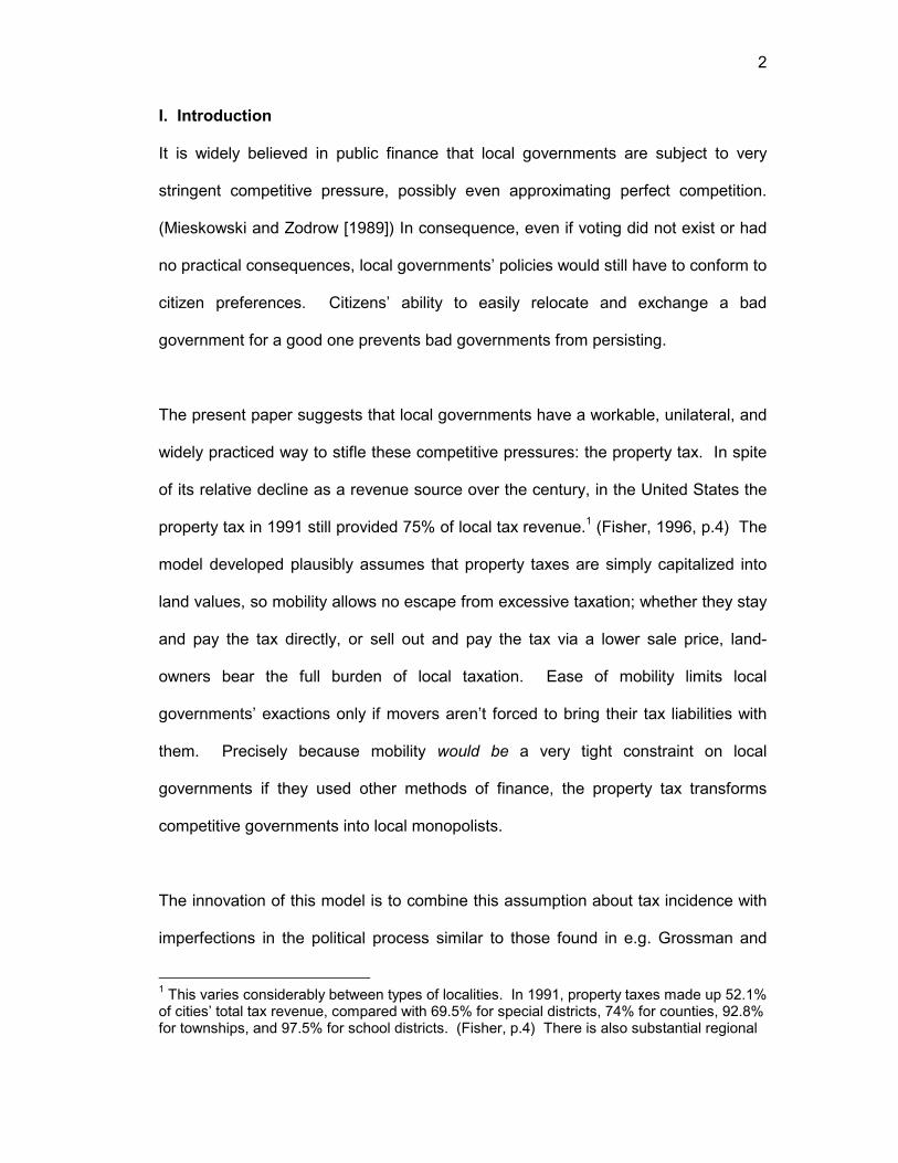
I. Introduction It is widely believed in public finance that local governments are subject to very

stringent competitive pressure, possibly even approximating perfect competition.

(Mieskowski and Zodrow [1989]) In consequence, even if voting did not exist or had

no practical consequences, local governments’ policies would still have to conform to

citizen preferences. Citizens’ ability to easily relocate and exchange a bad

government for a good one prevents bad governments from persisting.

The present paper suggests that local governments have a workable, unilateral, and

widely practiced way to stifle these competitive pressures: the property tax. In spite

of its relative decline as a revenue source over the century, in the United States the

property tax in 1991 still provided 75% of local tax revenue.1 (Fisher, 1996, p.4) The

model developed plausibly assumes that property taxes are simply capitalized into

land values, so mobility allows no escape from excessive taxation; whether they stay

and pay the tax directly, or sell out and pay the tax via a lower sale price, land-

owners bear the full burden of local taxation. Ease of mobility limits local

governments’ exactions only if movers aren’t forced to bring their tax liabilities with

them. Precisely because mobility would be a very tight constraint on local

governments if they used other methods of finance, the property tax transforms

competitive governments into local monopolists.

The innovation of this model is to combine this assumption about tax incidence with

imperfections in the political process similar to those found in e.g. Grossman and

1 This varies considerably between types of localities. In 1991, property taxes made up 52.1% of cities’ total tax revenue, compared with 69.5% for special districts, 74% for counties, 92.8% for townships, and 97.5% for school districts. (Fisher, p.4) There is also substantial regional

3

Helpman (1996). Under the special assumption of a perfectly functioning electoral

system, the model’s results are very similar to Tiebout’s. Yet the mechanism is quite

different: What actually forces local governments to conform to citizen preferences

in this model is voice, not exit. More importantly, insofar as the political process

works imperfectly, local governments have latitude to deviate from voters’

preferences.

This does not mean that different localities don’t cater to different tastes. The

subsequent model, like the Tiebout model, shows that it is natural and efficient for

people with similar tastes for public goods to reside in the same localities. But the

model differs from the Tiebout model in that it is political rather than economic

pressure which drives politicians to conform to voter preferences; in fact, the

economic pressure emphasized by the Tiebout model turns out to make no

difference.

The next section reviews some of the related literature. The third section sets up

the baseline model, in which imperfectly restrained politicians just waste or “eat”

extra taxes by extracting rents. The fourth section studies both the partial and

general equilibria of the baseline model. The fifth section extends the baseline

model to three germane topics: First, it investigates how the model works if rent-

extraction is capped at zero; the result is that politicians provide a higher level of

public goods than people desire. Second, it shows that if taxes attach to mobile

wealth rather than immobile land the economic constraints emphasized by the

Tiebout model reappear. The third part of the fifth section considers the model's

heterogeneity: property taxes ranged from a high of 98.2% of local tax revenues in New England, to a low of 68.2% for the Mideast. (Fisher, p.204)

4

implications for local constitutional design: property taxes probably have a minimal

excess burden, but they allow officials a great deal of latitude to oversupply public

goods; other taxes have a higher excess burden but place more effective

competitive restraints on policy-makers. The sixth section concludes the paper.

II. Related Literature

The present paper links several distinct strands of research, combining recent work

in political economy and electoral imperfections with the long-standing literature on

local public finance and tax capitalization. Tiebout (1956) inaugurated the modern

study of the local supply of public goods. This seminal paper broadly argued that

the market for local public goods potentially satisfied the assumptions of the

perfectly competitive model - many suppliers, perfect information, costless mobility,

and so on - and that in consequence local governments were tightly constrained to

adhere to citizen preferences even in the absence of democratic voting.2 Rose-

Ackerman (1983) provides both a useful summary of earlier literature and raises a

number of other important issues on the interaction of political and economic forces

in local public finance.

The limitations of the Tiebout model are emphasized in an influential paper by Epple

and Zelenitz (1981). In their model, local governments engage in Tiebout-style

competition with each other, but face no internal political competition (such as

elections). In this setting, Epple and Zelenitz conclude, inter-jurisdictional

competition cannot fully eliminate the monopoly power of local governments. The

implication is that democratic control over government may matter somewhat even

5

on the local level. My model differs from that of Epple and Zelenitz in two ways.

First, whereas Epple and Zelenitz show that Tiebout-type competition is not fully able

to eliminate local government's monopoly power, my model actually concludes that

Tiebout competition does not reduce the monopoly power of local governments at

all. Second, while Epple and Zelenitz show that economic competition without

political competition yields less-than-perfectly competitive results, my model shows

that even if economic competition is supplemented by political competition, local

governments will (except in certain polar cases) fall short of the perfectly competitive

ideal.

Mieskowski and Zodrow label Tiebout's view of local public finance the "benefit tax"

view, to which they contrast the so-called "new view" in which the property tax is

essentially a distortionary tax on capital. "New view" models typically assume a fixed

but mobile capital stock rather than a fixed and immobile land stock. Land also

assumes a central role in the literature on the "Henry George Theorem," discussed

in such works as Arnott and Stiglitz (1979) and Boadway and Flatters (1982).

Yinger, Bloom, Börsch-Supan, and Ladd (1988) thoroughly review the literature on

tax capitalization without, however, considering the implications of tax capitalization

for the effectiveness of Tiebout-style competition. One of the very few papers to

explore the interaction between capitalization and local political economy is Yinger

(1985); he concludes, for reasons rather different than those in the present paper,

that capitalization normally leads to excessive local government expenditure.

2 For more details and numerous extensions of the Tiebout model, see Mieszkowski and Zodrow (1989), Zodrow (1983), and Thisse and Zoller (1983).

6

Most of the literature on imperfections in the voting process is comparatively recent;

Inman (1988) provides a good survey of earlier work. The specific imperfection

used here resembles one introduced in Lindbeck and Weibull (1987), and more

recently in Dixit and Londregan (1995a), Dixit and Londregan (1996), and Grossman

and Helpman (1996). (Although for a skeptical view of the "political failure"

literature, see Wittman [1995]). In these models, parties may easily alter their

positions on some issues (such as budgetary issues), but not their positions on other

issues (such as abortion). This structure somewhat weakens the competition

between the parties, allowing deviations from the preferences of the median voter to

occur in equilibrium. The present model formalizes the imperfection in the voting

process as a pure preference for party loyalty, though this could be interpreted as

arising from the existence of "uninformed" and "informed" voters as in Grossman

and Helpman (1996), or Baron (1994).

A recent paper by Nechyba (1997) also explores the interaction between economic

and political constraints upon local governments, although his model and technique

differ considerably from that of the present paper. Nechyba develops a general

equilibrium simulation in which local governments require the aid of an outside

enforcer (such as a common state government) to jointly deviate from property taxes

to income taxes. But in his model is it necessary to appeal to citizens' exogenous

perception of the unfairness of property taxation to explain the motive for joint

deviation, because collusion significantly increases neither voters' nor politicians'

utility. In contrast, in the present model property taxes are actually a perfectly

efficient way to raise a given amount of revenue for local public spending, but voters

may dislike property tax regimes because they can lead to excessive tax rates.

7

III. The Baseline Model

A. The Political Setting

There are N localities, indexed by {1, 2, ..., k , ... N }. (Note that the interpretation of

all symbols used is given in Table 1). Within each locality are two competing

political parties i and j. The utility of party i is given by:

)(* kii GVIu θµ += (1)

where iI is an indicator variable which is 1 if party i wins the election and zero

otherwise; kG is the size of the government (funded by property taxes) in locality k ;

µ is taxation in excess of that necessary to supply public goods level kG ; θ <1, and

0(.)' >V . Intuitively, the party in power gains utility from both power and rents, but is

willing to trade off power for rents. Party j’s utility is defined similarly. Thus the

model follows Wittman (1977) in assuming that politicians care about policy as well

as electoral victory.

The local governments are in principle under the control of a single state

government, but for current purposes we ignore the political and economic

pressures on that state government. Each locality has a fixed supply of land,

designated Lk . L Lkk

N

=

≡1

. Thus we are imagining a relatively developed situation,

in which surplus land (or an “urban fringe”) no longer exists; land is a fixed stock with

a vertical supply curve. Moreover, the land within each locality is fixed because the

borders are set exogenously; for simplicity, assume that each locality has the same

8

amount of land, NLLk = . Finally, there is assumed to be perfect mobility between

localities. Retaining this strong Tiebout entry/exit assumption helps to illuminate how

powerfully the method of tax finance can alter the competitiveness of local

governments.

B. Households and Their Utility Functions

Within the state, there are F households comprised of equal numbers of N

different types, indexed by {1, ..., s ,... N }; hence, there are NF / households of

each type s . The types mainly differ from one another in the intensity of their taste

for public goods, as shall be explained below. Households enter the game with an

equal endowment of immobile land fL ; somebody has to own all of the land, so

L Lff

F

=

=1

. For simplicity, we normalize the total stock of land to equal F ; thus

each household has 1 unit of land and each locality has a NF / units of land in it.

Aside from their land endowment, households have liquid wealth, fW , which can be

consumed or used to buy capital goods to combine with land and produce housing.

Each voter has a taste for parties as well as policies; designate this party preference

fρ . fρ essentially measures how much utility agents are willing to give up in order

to live under their preferred party, so that an agent f votes for party i instead of

party j iff:

jfif

if uIu ≥+ ρ (2)

9

where ifu is the utility that agent f would derive from party i’s policies, and j

fu is

the utility f would derive from party j’s policies.

The only distributional assumption about the party preference is that fρ >0 for all

households.3 Intuitively, this means that party i is the “advantaged” party: if the

parties offer identical platforms, all voters prefer party i.4

Each household has a quasi-linear utility function assumed to follow:

fffkf CHHGUu ++= ln)( (3)

That is, households gain utility from the housing they occupy, the level of

government services their locality supplies to them (assumed to be proportional to

one’s quantity of housing), and from consumption out of the wealth remaining after

paying for housing and local taxes. Note that it is assumed that it is only possible to

live in and derive utility from housing and services in one locality, and that utility is an

increasing function of government services, so dU GdG

( ) > 0 . Due to the quasi-linear

form of the utility function (and assuming an interior solution) one can ignore the

income effects of price changes on housing demand.5

3 The assumption that fρ is non-negative for all voters is not necessary for the results, but it considerably simplifies the analysis of voters’ locational choices. 4 Slightly different analyses of imperfections in the electoral process include Baron (1994), Dixit and Londregan (1995a; 1996), and Grossman and Helpman (1996), while Peltzman (1992) provides some empirical evidence for the importance of imperfections in the political process. 5 Allowing different utility specifications merely amplifies the conclusion of the model; in a more standard utility function with an income effect, the result of a property tax is in fact over-capitalization. The reason is that a property tax reduces wealth, which normally reduces

10

Let )(GT designate the per-housing-unit level of taxes necessary to supply the per-

housing-unit level of services G , 10 ≤≤ G ; and let µ indicate the level of taxation

in excess of that necessary for service level G . With all revenue drawn from

property taxation, it is then by definition true that:

t p T Gk kH

k k= +( ) µ (4)

Each citizen has a most preferred level of services,Gf : Below that point providing

services at marginal cost increases the citizen’s utility, while above that point

services delivered at marginal cost decrease the citizen’s utility. It is convenient to

formalize this using the following functional form:

fkkk GGZGTGU −−=− )()( (5)

Gk gives the actual level of such public services in locality k . Z is the value (5)

takes on when the actual tax-and-service package is at the agent’s personal

optimum level.

Gf distinguishes the N different types of households from one another. The taste

of the type indexed Ns = , with the greatest taste for public goods, is designated

G ; the tastes of the N different types are distributed according to:

NsGNsGs ,...3,2,1 ==

(6)

housing demand even further; with a fixed housing stock, housing values fall by 100% of a property tax increase due to capitalization, and by somewhat more due to the income effect of the property tax.

11

Assume that citizens are initially “sorted” by tastes.6 The NF / households with the

lowest taste for public goods, indexed by s =1, reside in and own their endowment of

land in locality k =1, the NF / households with the second lowest cluster of tastes

for public goods, indexed by s =2, reside in and own their endowment of land in

locality k =2, and so on. Thus, the price of land in a household’s initial locality enters

into its budget constraint. Finally, the price of consumption is assumed to be fixed at

1 by the national market, so a household’s budget constraint is given by:

Lkfff

Hkk pWCHpt +≤++ )1( (7)

C. The Housing Stock

The housing stock is produced by combining land and capital goods. Empirically,

estimates of tax capitalization often reach or even exceed 100%.7,8 (Yinger et al.

[1988]) The production function and supply elasticities used here are picked to be

consistent with this fact.

There is a Leontief fixed-proportions production function, so for any locality k :

H FN

Kk k= min{ , }β (8)

6 It will later be shown that this assumption of ex ante sorting is unnecessary; it simply makes it easier to understand how the model works. 7 As Yinger et al. (1988) notes, estimated capitalization rates below 100% may be largely due to the fact that tax differentials are rarely permanent. Rates above 100% are theoretically possible insofar as property taxes impose a dead-weight loss via the taxation of structural improvements. Another important difficulty in estimating the degree of tax capitalization is the selection of the appropriate risk-adjusted discount rate. 8 See also Martinez-Vasquez and Ihlanfeldt (1987) which finds serious econometric deficiencies (although no consistent positive or negative bias) in most of the empirical work on tax capitalization.

12

Land, as explained earlier, is a fixed, immobile stock and is supplied perfectly

inelastically. The supply of capital goods, however, is perfectly mobile, so Kp is

fixed. Then assuming that no land is left idle, FK =β .

Housing is produced competitively, so the before-tax price of one unit of housing is

equal to the cost of production:

β

KLk

Hk

ppp += (9)

IV. Equilibrium in the Baseline Model

We first put forward a candidate equilibrium for the housing market and political

tournament considering a given locality in isolation. After examining this partial

equilibrium of N autarchic communities, it will be shown that due to the presence of

tax capitalization, the existence of alternative localities will not induce re-location in

the face of tax differentials. In short, we will investigate partial equilibria in N

localities, then prove that this is the same as the general equilibrium for N localities.

A. Partial Equilibrium in the Economic and Political Game

First consider the economic and political game without mobility. Equilibrium in each

locality considered in isolation requires that:

1. No citizen may desire to vote differently.

2. No party may desire to offer a different platform.

Consider a candidate partial equilibrium with the following properties: First, both

parties offer to satisfy exactly the most preferred level of kG of their constituents

(remembering that at least ex ante, the inhabitants of each locality have identical

13

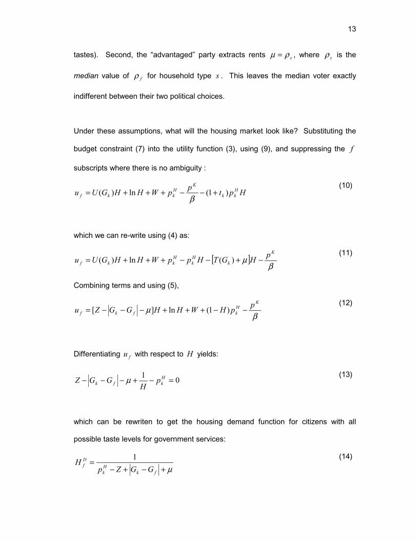
tastes). Second, the “advantaged” party extracts rents sρµ = , where sρ is the

median value of fρ for household type s . This leaves the median voter exactly

indifferent between their two political choices.

Under these assumptions, what will the housing market look like? Substituting the

budget constraint (7) into the utility function (3), using (9), and suppressing the f

subscripts where there is no ambiguity :

HptppWHHGUu Hkk

KHkkf )1(ln)( +−−+++=

β

(10)

which we can re-write using (4) as:

[ ]β

µK

kHk

Hkkf

pHGTHppWHHGUu −+−−+++= )(ln)( (11)

Combining terms and using (5),

βµ

KHkfkf

ppHWHHGGZu −−+++−−−= )1(ln][ (12)

Differentiating fu with respect to H yields:

01 =−+−−− Hkfk p

HGGZ µ

(13)

which can be rewriten to get the housing demand function for citizens with all

possible taste levels for government services:

µ+−+−=

fkHk

Df GGZp

H 1

(14)

14

Remembering our assumption that each type of citizen has identical tastes for public

goods, it becomes possible to derive the overall demand schedule for housing within

a locality.

µ+−+−=

skHk

Dk GGZpN

FH 1

(15)

Setting housing demand equal to the fixed housing supply NF / shows us that:

NF

GGZpNF

skHk

=+−+− µ

1

(16)

solving (16) for the price of housing in locality k , we learn that:

skHk GGZp −−−+= µ1 (17)

Note that (17) shows that tax payments in excess of the cost of providing a given

level of government services are fully capitalized into the price of housing.

Moreover, since this candidate equilibrium stipulates that G Gk s− =0, and sρµ = :

kZp sHk ∀+=+ 1ρ (18)

In other words, before-tax housing prices, adjusted for rent-extraction, will be

identical for all localities if the winning political parties equate actual and desired

levels of public goods for each locality.

15

Now consider the effects of the candidate equilibrium political platform on the

housing market. Agents’ utility in their initial locality is given by:

[ ]β

ρK

Hk

Hksf

ppWHHpZu −+++−−= ln (19)

Substituting in for housing prices given the level of government services yields:

βρ

K

sfpWZu −+−=

(20)

Now consider whether this candidate partial equilibrium is actually an equilibrium.

The housing market’s operation is clearly an optimal response given the political

policies; but are these political policies optimal choices for voters and political

parties?

Citizens without any party allegiance vote for whichever party gives them the highest

utility level in terms of services and taxes. Thus, if 0=sρ , the only possible political

equilibrium would be one in which both parties offer platforms with µ =0 and

G Gk s− = 0 .

However, so long as 0≠sρ , the story is more complicated. The advantaged party

clearly wins the election if both parties offer platforms with µ =0 and G Gk s− = 0 ;

moreover, due to its supermajority, the advantaged party can still win the election if it

somewhat increases either kG or µ (and thereby strictly increase its own utility). In

16

fact, it wins the election with probability 1 so long as the utility loss from the

combined excess kG and µ is less than sρ .

Which mix of excess kG and µ will the advantaged party pick? The utility effects

on citizens are identical (by equations [17] and [19]). However, by equation (1),

k

i

k

ii

Gu

Guu

∂∂

∂∂

θ∂µ∂

>= 1, so the best way for a party to take its advantage is always in

the form of rents if this is allowed.

The candidate equilibrium for this political game can thus be seen to be a full-

fledged equilibrium. An advantaged party always wins if it plays µ =0 and

G Gk s− = 0 , but it if did so it would not be taking full advantage of the situation.

Given an unconstrained choice between the two margins of increased government

size or increased rents, party i can get the most utility by simply taking 100% of its

advantage in the latter form. The result of this process is that housing prices

perfectly capitalize politicians’ rent-extraction; the entire burden of imperfect political

competition is borne by the housing sector.

B. General Equilibrium in the Housing Market

To determine the general equilibrium in the overall economic and political game, it

will be necessary to meet three conditions:

1. No citizen may desire to move to another locality.

2. No citizen may desire to vote differently.

3. No party may desire to offer a different platform.

17

The investigation of general equilibrium with costless movement begins with the

preceding analysis of partial equilibrium in which relocation was impossible. The

perhaps surprising result is that the general equilibrium in the game with relocation is

the same as the partial equilibrium in the game without relocation. The argument

proceeds by showing that the partial equilibrium satisfies all three conditions for

general equilibrium.

Equilibrium Condition #1

An agent’s utility from remaining in his initial locale is given by:

βµ

KHk

Hkf

ppWHHpZu −+++−−= ln][ (21)

Which we may compare to the utility which would be derived from residing in a

different locale:

βµ

KHk

Hkfkf

ppWHHpGGZu −++′+′−′−−−=′ ′′ ln][ (22)

Substituting in for pkH and pk

H′ using (17) into equation (12), it may be seen that:

βρ

βρ

K

sfkf

K

sf

pZWGGu

pZWu

−−++−+−=′

>−−+=

′′ )1ln(

(23)

Inequality (23) shows that the partial equilibrium described earlier satisfies the first

condition for general equilibrium. Holding other aspects of the game constant,

opening up alternative localities creates no incentive to move. How is this possible?

18

Essentially, because an excessive charge for services is borne entirely by the

original landowners, regardless of whether they opt to remain or migrate. Given the

presence of political rent-extraction, there is no incentive to migrate. All that this

would accomplish would be to change the level of government services without in

the slightest mitigating the lost wealth due to the excessive charge for government

services in one’s original locality.

Equilibrium Condition #2

Would any voter wish to alter his or her voting decision once movement between

localities is possible? After all, it is no longer necessarily true that voters will vote for

the candidate that best satisfies their own tastes for services and taxes; rational

voters, being home-owners as well, will want to consider the effect of different

policies on their wealth via housing prices as well as their own comfort. Leaving

aside party allegiances, citizens vote for whichever party gives them the most utility;

do the changed conditions change voters’ most preferred policies?9

The answer is no. Using (23), it can be seen that a citizen from locality 'k could

only be induced to relocate if the quantity of housing they would demand in the other

locality would increase.

fkHk

Hk GGpp −>−' (24)

That is, the price in the other locality must be sufficiently below the price in their

locality of origin to compensate for the less-preferred tax-and-service package. This

is turn would occur only if the price in k fell below the price in k ′ :

19

Zp sHk +<+ 1ρ (25)

But from (21), it can be seen that the inhabitants of k would only try to induce

migration if it would result in:

Zp sHk +>+ 1ρ (26)

Since (25) and (26) are never both satisfied, citizens in k must have no incentive to

vote for different policies. Even in the polar case where a locality exactly adopted

the most-preferred policies of, for example, an attitudinally adjacent locale (i.e.,

where preferences differed by NG

) in order to induce migration, the result would

merely be a lower housing price for both localities:

2

1

221

2

'

+�

���

�

+−+=+=+ ′

NG

NGZpp s

Hks

Hk ρρ

(27)

Note that the limit of the above expression as ZNG +=→ 10 ; i.e., even if there

were an infinite number of localities, it would still be impossible to raise sHkp ρ+

above its candidate equilibrium value of Z+1 . Hence we have shown that the

proffered candidate equilibrium satisfies the second equilibrium condition: No voter’s

preferred policies and hence voting decisions would change relative to their

preferences and voting in partial equilibrium.

9 Voting occurs before movement occurs, ensuring that a given citizenry cannot be pushed

20

Equilibrium Condition #3

Finally, would any candidate wish to offer a different platform? Again, the answer is

no (assuming, as we do, that migrants must wait a period before they can vote; or in

other words, politicians must win the support of current citizens for their policies

before they can implement them). The advantaged party and its margin of

advantage remain unchanged. Similarly, its two ways of enjoying its advantaged

position and their respective marginal benefits don’t change either. The partial

equilibrium argument goes through unchanged.

By checking these three equilibrium conditions, it has been shown, perhaps

surprisingly, that the Nash equilibrium for N isolated localities (pre-sorted by

preferences) is exactly the same as the Nash equilibrium for those same N

localities with perfect mobility.

Even though landowners bear excessive property tax burdens, interlocal competition

in some sense persists. Suppose that the tastes of a small portion of the population

in one locality change (as in the standard example in which a family’s taste for public

goods increases once it has school-age children). It would still make sense for this

household to move to a locality that better matched their preferences. However, this

is not migration in response to excessive charges for a set service level; it is

migration in response to a change in the desired service level.

In this model, what precludes local governments from charging exorbitant fees for a

given service package is not the option of moving. Moving does nothing to eliminate

out by migration-inducing policies unless they themselves desire it.

21

such burdens, which are merely capitalized into sale values. Rather, it is the

electoral constraint which keeps local governments in line. If sρ =0, then the

electoral system perfectly constrains politicians to supply exactly the desired service

level at the minimum cost. But if the electoral system deviates from this condition

(i.e., if voters have some party loyalties), then the restraints on politicians will not be

strong enough to prevent them from exercising some degree of monopoly power. If

there were no elections, i.e., if local governments were (malevolent) dictatorships,

the presence of nearby alternative communities would not prevent full expropriation

of land-owners via the property tax. The resulting equilibrium would look very much

like a polar case considered in Epple and Zelenitz (1981), where local dictatorships

extract rents from perfectly immobile tax bases.

C. Does the Ex Ante Sorting Assumption Matter?

It was assumed that citizens are pre-sorted by taste levels. Is the equilibrium of the

overall game driven by this seemingly strong assumption? Perhaps surprisingly, this

assumption makes no difference whatever, serving merely to simplify the

presentation. In this section, it is proven that the same equilibrium would arise for

any arbitrary initial distribution of land holdings. That is, regardless of the ex ante

endowments of land, in equilibrium citizens must be sorted according to their taste

levels.

Suppose that citizens are not initially sorted according to tastes, but that equal

numbers of citizens NF / initially reside in each locality. It is impossible for such a

situation to satisfy our Equilibrium Condition #1, because there will necessarily be

gains to trade. Assume that there exist at least two “misplaced” agents A and B

22

such that A resides in locality k and B resides in locality 'k , but

G G G Gk A k A− > −' and G G G Gk B k B' − > − .

Note first the agents’ respective utilities in their initial locale:

βρ

KHkBAA

HksAk

Ak

ppWHHpGGZu −+++−−−−= ln][ (28)

[ ]β

ρK

HkBBB

HksBk

Bk

ppWHHpGGZu −+++−−−−= ''''' ln (29)

Consider the utility of the two agents if they simply swapped their locations:

βρ

KHkBBB

HksAk

Ak

ppWHHpGGZu −+++−−−−= ''''' ln][ (30)

βρ

KHkBAA

HksBk

Bk

ppWHHpGGZu −+++−−−−= ln][ (31)

But note that:

( )( ) ( ) 0

)(

''

''

>−−−+−−−=+−+

BAkBkABkAk

Bk

Ak

Bk

Ak

HGGGGHGGGGuuuu

(32)

Given the quasi-linear utility specification, this implies that there must exist a

mutually beneficial trade; wealth transferred between bargainers reduces the utility

of the giver by the same amount that it increases the utility of the receiver. The

23

assumption of ex ante sorting turns out to be innocuous, and can be used without

loss of generality.

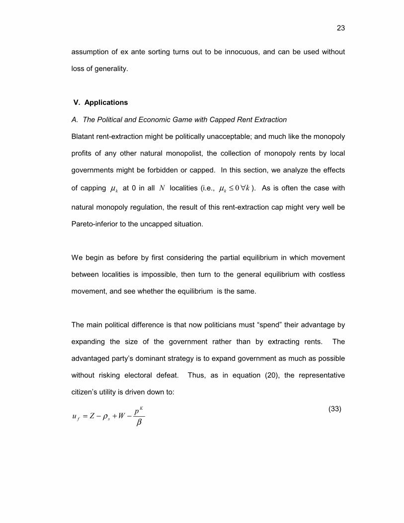
V. Applications

A. The Political and Economic Game with Capped Rent Extraction

Blatant rent-extraction might be politically unacceptable; and much like the monopoly

profits of any other natural monopolist, the collection of monopoly rents by local

governments might be forbidden or capped. In this section, we analyze the effects

of capping kµ at 0 in all N localities (i.e., kk ∀≤ 0µ ). As is often the case with

natural monopoly regulation, the result of this rent-extraction cap might very well be

Pareto-inferior to the uncapped situation.

We begin as before by first considering the partial equilibrium in which movement

between localities is impossible, then turn to the general equilibrium with costless

movement, and see whether the equilibrium is the same.

The main political difference is that now politicians must “spend” their advantage by

expanding the size of the government rather than by extracting rents. The

advantaged party’s dominant strategy is to expand government as much as possible

without risking electoral defeat. Thus, as in equation (20), the representative

citizen’s utility is driven down to:

βρ

K

sfpWZu −+−=

(33)

24

only now citizen utility is below its optimum because µ =0 and G Gk s s− = ρ , rather

than having sρµ = and G Gk s− = 0 . The effect on housing prices is clear; using

equation (17),

skHk GGZp −−+= 1 (34)

implying that:

kZGGp skHk ∀+=−+ 1 (35)

The partial equilibrium effect of the cap falls entirely upon politicians. Citizens’ utility

is not improved, but the welfare of the winning party is now u V Gi f s= +( )θ θρ rather

than u V Gi f s= +( )θ ρ as it was before the introduction of the cap.

A more complicated proof omitted here shows that this partial equilibrium will also be

a general equilibrium so long as sNG

s ∀< 2

ρ . Intuitively, there are no gains to

trade until the size of government in locality k is closer to the preferred size of non-

residents than it is to the size of residents.

B. The Political and Economic Game with Non-Property Taxes

This section considers the effects of replacing the property tax with some method of

finance which will not perfectly capitalize into housing values. In particular, it

illustrates that Tiebout-type mobility checks on local government reappear under

alternative tax regimes. If local political competition is completely ineffective, or if

25

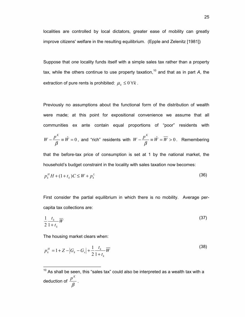
localities are controlled by local dictators, greater ease of mobility can greatly

improve citizens' welfare in the resulting equilibrium. (Epple and Zelenitz [1981])

Suppose that one locality funds itself with a simple sales tax rather than a property

tax, while the others continue to use property taxation,10 and that as in part A, the

extraction of pure rents is prohibited: kk ∀≤ 0µ .

Previously no assumptions about the functional form of the distribution of wealth

were made; at this point for expositional convenience we assume that all

communities ex ante contain equal proportions of “poor” residents with

0ˆ =≡− WpWK

β, and “rich” residents with 0ˆ >=≡− WWpW

K

β. Remembering

that the before-tax price of consumption is set at 1 by the national market, the

household’s budget constraint in the locality with sales taxation now becomes:

p H t C W pkH

k kL+ + ≤ +( )1 (36)

First consider the partial equilibrium in which there is no mobility. Average per-

capita tax collections are:

12 1ttWk

k+

(37)

The housing market clears when:

Wtt

GGZpk

ksk

Hk +

+−−+=12

11 (38)

10 As shall be seen, this “sales tax” could also be interpreted as a wealth tax with a

deduction of β

Kp.

26

Under the property tax regime, there was unanimity within each locality on the

appropriate supply of public goods. But now that a sales tax funds public goods, the

utility of poor households is given by:

Wtt

GWWtt

GZuk

ks

k

kf +

+−�

���

�+

+−=

121)(

121

(39)

where )(TG indicates the inverse of )(GT i.e., )(TG gives the highest level of G

which may be supplied from a given amount of taxation.

Similarly, the utility of rich households is given by:

Wt

tGWW

tt

GZuk

k

sk

kf +

++−

����

�+

+−=

1211

)(12

1

(40)

There will no longer be unanimous agreement that the government ought to set

G Gh s= ; with taxation of unequal wealth funding equal benefits, the poorer citizens

will most prefer G Gh s> ; similarly the richer type will most prefer G Gh s< . In

particular, due to the stark assumption that 0=W for half of the population (and

because dU GdG

( ) > 0 ), there is every reason for the low-wealth type to favor full

expropriation of the wealthier type by setting t k = ∞ . With half of the population of

the low-wealth type, the political partial equilibrium is extremely simple: the

advantaged party wins with exactly 50% of the vote and sets G G Wk = � �

2 In short,

with sales taxes and no mobility, the wealthier citizens can be easily expropriated

27

through the democratic process, but receive the same level of services as everyone

else.

The situation changes in general equilibrium with mobility between communities. It

then becomes possible for the wealthy type of citizen to sell their housing to low-

wealth types from other localities and take their wealth with them. For example, if

NkGWGk

12

+=�

���

� there is an incentive for the wealthy citizens of locality k to switch

places with the poor inhabitants of locality 1+k . By trading places, the wealthy

migrants will be able to obtain public services without paying for twice the services

they receive. Clearly this is not a stable equilibrium; to prevent the out-migration of

the wealthy citizens, it would be necessary to ensure that they prefer their original

abode to the next best alternative:

WWtt

NGsZu

Wt

tGWW

ttGZu

k

kk

k

k

sk

kk

++

+−=

>+

++−

����

�+

+−=

121

1211

)(12

1

'

(41)

which implies the following incentive compatibility condition:

WNGsGWW

ttG

tt

sk

k

k

k >�

���

�+−��

�

���

+

+−

+)(

1211

(42)

which seriously limits the possibility of local redistribution. Much as in the Tiebout

model, when local taxes attach to mobile resources rather than immobile property,

28

the existence of convenient alternative communities makes a large political

difference, supplementing or even supplanting electoral constraints.

C. Local Constitutional Choice and Time Consistency

A central goal of constitutional choice is to solve the time-consistency problem to

eliminate or guard against ex post incentives to defect from ex ante optimal

strategies. (Kydland and Prescott [1977]; Barro and Gordon [1983]; Fisher and

Summers [1989]) The preceding analysis of the methods of local taxation suggest

that the time consistency problem for local government could be particularly severe.

Property taxation has a very low excess burden; in fact, in the model outlined in the

paper, property taxation permits costless transfers from citizens to the government.

Unfortunately, precisely because property taxation raises revenue so efficiently, it

leaves citizens vulnerable to expropriation ex post.

Just as a lower dislike of inflation can cause lower utility in equilibrium in strategic

situations between central bankers and the public (Rogoff [1985]), so too can a

lower cost of expropriation reduce utility in strategic situations between local

governments and homeowners. The deadweight burden of sales or income tax

might be considerably greater than that of the property tax, but the attendant flight of

businesses and high-income residents makes expropriation less attractive ex post.

It is possible to eliminate the incentive for expropriation by capping the rents that the

government can charge. This is the approach that most modern democracies

without serious corruption problems typically select. However, capping permissible

rent-extraction can create a second problem: since they cannot take the rents

29

directly, politicians may take them indirectly by expanding the size of the public

sector over which they preside. This can be inefficient, since it could easily lead

politicians to supply public goods that the citizenry does not value above their

marginal cost.

Local constitutions therefore normally choose between two possible kinds of

inefficiency: the inefficiency of distortionary tax systems, and the inefficiency of

supply of public goods valued below their cost. The property tax system minimizes

tax distortion, but makes it very easy to expand the size of local governments. Non-

property taxes, in contrast, can be very distortionary, but this very fact checks the

expansion of the public sector.

VI. Conclusion

Many public finance economists believe that local governments face a stringently

competitive environment. On its face, this view is plausible: relocation is always an

option for a local government’s dissatisfied customers. This paper reverses the

standard conclusion. Mobility doesn’t matter if an unwanted tax burden moves with

you.

The model presented here does give some predictions similar to the traditional

Tiebout model. In both models, localities specialize in satisfying different kinds of

tastes; people with similar tastes naturally tend to reside in the same areas.

Similarly, if a person’s tastes change, both the current model and the Tiebout model

would predict that they would relocate to a new location which served a public goods

package closer to their desired level. Both the Tiebout model and the current model

30

see that tastes for service differ among people, so local governments differentiate

their product to appeal to these diverse tastes.

There are, however, two crucial differences. First, the Tiebout model sees economic

competition as the primarily check upon local governments. The model presented

here indicates that economic competition makes very little difference for local

governments; instead, what matters is how well the electoral system works. If the

electoral system works well, it is possible to enjoy the low deadweight loss of

property tax funding without risking excess supply of public goods; but as the

imperfections in the electoral system increase, the low deadweight loss of the

property tax simply makes it easier to inefficiently expand the size of the public

sector.

The second important difference is that while the Tiebout model can be first-best

efficient under many assumptions (Mieskowski and Zodrow [1989]), the current

model shows that there is considerable room for inefficiency in local governments.

Property owners, rather than the government, bear the burden of excessive charges

for public goods; the only check on abuse is to elect a different party. Local politics

is all politics; what determines the efficiency of the local public sector is not the ease

of relocation, but the severity of the imperfections in the political process.

31

Table 1: A Summary of the Model

Exogenous

Variables

Interpretation

N number of localities and types of citizens

k index for localities

θ taste parameter; 0<θ <1 ρ magnitude of a citizen’s party preference; measures how much utility

an agent is willing to give up in order to live under preferred party

Lk fixed supply of land in locality k

L total supply of land

F number of households s index for citizen types

Lf initial land endowment of household f

Wf initial liquid wealth endowment of household f

Gf most preferred public service level of household f

Z value of )()( GTGU − when service provision is at an agent's

personal optimum

T Gk( ) per-housing unit level of taxes necessary to provide public service

level Gk

G most-preferred service level of citizen type with highest taste for public

goods

β parameter in housing production function

�W wealth minus cost of capital goods used to build housing

W �W of "rich" citizens

W �W of "poor" citizens

G T( ) highest level of G which may be supplied from a given amount of

taxation

32

Endogenous

Variables

Interpretation

ui utility function of party i

Ii indicator variable=1 if party i wins, =0 otherwise

V Gk( )µ θ+ utility of party in locality k conditional on ruling

Gk public goods level in locality k

u f utility of household f

U H Gf k( , ) level of utility of household f derived from housing and local services

fC level of household consumption of household f

H f level of housing consumed by household f

t k tax rate in locality k

pkH housing price in locality k

µ k per-housing-unit taxation in excess of that necessary to provide

public goods level Gk

pkL land price in locality k

Hk housing production in locality k

Kk capital goods used to produce housing in locality k

pK price of capital goods

H fD housing demanded by household f

33

References

R. Arnott, and J. Stiglitz, Aggregate land rents, expenditures on public goods, and

optimal city size, Quarterly Journal of Economics, 43, 471-500 (1973).

D. Baron, Electoral competition with informed and uninformed voters, American

Political Science Review, 88, 33-47 (1994).

R. Barro, and D. Gordon, A positive theory of monetary policy in a natural rate

model, Journal of Political Economy, 41, 589-610 (1983).

R. Boadway, and F. Flatters, Efficiency and equalization payments in a federal

system of government: a synthesis and extension of recent results, Canadian

Journal of Economics, 15, 613-33 (1982).

A. Dixit, and J. Londregan, Redistributive politics and economic efficiency, American

Political Science Review, 89, 856-66 (1995a).

A. Dixit, and J. Londregan, The determinants of success of special interests in

redistributive politics, Journal of Politics, 58, 1132-1155 (1996).

D. Epple, and A. Zelenitz, The implications of competition among jurisdictions: does

tiebout need politics?, Journal of Political Economy, 89, 1197-1217 (1981).

G. Fisher, "The Worst Tax? A History of the Property Tax in America," University

Press of Kansas, Lawrence (1996).

S. Fischer, Stanley, and L. Summers, Should governments learn to live with

inflation?, American Economic Review, 79, 382-387 (1989).

G. Grossman, and E. Helpman, Electoral competition and special interest politics,

Review of Economic Studies, 63, 265-86 (1996).

34

R. Inman, Markets, government, and the ‘new’ political economy, in "Handbook of

Public Economics" (A. Auerbach and M. Feldstein, Eds.), North Holland, Amsterdam

(1988).

F. Kydland, and E. Prescott, Rules rather than discretion: the inconsistency of

optimal plans, Journal of Political Economy, 85, 473-91 (1977).

A. Lindbeck, and J. Weibull, Balanced-budget redistribution as the outcome of

political competition, Public Choice, 52, 273-97 (1987).

J. Martinez-Vasquez, and K. Ihlanfeldt, Why property tax capitalization rates differ:

a critical analysis, in "Perspectives on Local Public Finance and Public Policy," vol.

3 (J. Quigley, Ed.), JAI Press, Greenwich (1987).

P. Mieszkowski, and G. Zodrow, Taxation and the tiebout model: the differential

effects of head taxes, taxes on land rents, and property taxes, Journal of Economic

Literature, 27, 1098-1146 (1989).

T. Nechyba, Local property and state income taxes: the role of interjurisdictional

competition and collusion, Journal of Political Economy,105, 361-84 (1997).

S. Peltzman, Voters as fiscal conservatives, Quarterly Journal of Economics, 107,

327-361 (1992).

K. Rogoff, The optimal degree of commitment to an intermediate monetary target,

Quarterly Journal of Economics, 100, 1169-1190 (1985).

S. Rose-Ackerman, Tiebout models and the competitive ideal: an essay on the

political economy of local government, in "Perspectives on Local Public Finance and

Public Policy," vol.1 (J. Quigley, Ed.), JAI Press, Greenwich (1983).

J. Thisse, and H. Zoller, Eds., "Locational Analysis of Public Facilities," North

Holland, Amsterdam (1983).

35

C. Tiebout, A pure theory of local expenditures, Journal of Political Economy, 64,

416-424 (1956).

D. Wittman, Candidates with policy preferences: a dynamic model, Journal of

Economic Theory, 14, 180-189 (1977).

D. Wittman, "The Myth of Democratic Failure: Why Political Institutions are Efficient,"

University of Chicago Press, Chicago (1995).

J. Yinger, H. Bloom, A. Börsch-Supan, and H. Ladd, "Property Taxes and House

Values: The Theory and Estimation of Intrajurisdictional Property Tax Capitalization,"

Academic Press, New York (1988).

J. Yinger, Inefficiency and the median voter: property taxes, capitalization, and the

theory of the second best, in "Perspectives on Local Public Finance and Public

Policy," vol.2, (J. Quigley, Ed.), JAI Press, Greenwich (1985).

G. Zodrow, Ed., "Local Provision of Public Services: The Tiebout Model After

Twenty-Five Years," Academic Press, New York (1983).