standing wave pattern for tx lines
DESCRIPTION
Transmission lines, Standing Wave, PatternTRANSCRIPT

Transmission Lines and E.M. Waves Prof R.K. Shevgaonkar
Department of Electrical Engineering Indian Institute of Technology Bombay
Lecture-9
Welcome, we have been discussing the Transmission Lines and its application for various
things like identifying loads or measurement of load impedance and so on. In this lecture
we will see if we know the standing wave pattern for a particular load termination on the
Transmission Line then how quickly we should identify the type of load. We have seen
that depending upon the load which is terminated on the line the standing wave pattern is
set up on Transmission Line and standing wave pattern has two characteristic parameters,
one is the location of the minimum from the load end of the Transmission Line and
second one is the voltage standing wave ratio.
So essentially looking at the standing wave pattern and then using the parameters at the
location of voltage or current minimum and the voltage standing wave ratio we can
quickly identify the type of the load. So essentially without really calculating the quantity
voltage standing wave ratio the idea here is to quickly identify the type of the load. We
are not interested here in finding out what is the exact value of the load but just if I
quickly glance at the standing wave pattern then how do we identify the type of the load.
So here we will look at two quantities, one is the location of voltage minimum on the
standing wave pattern and second one we will look at is the quantity called the VSWR.
As we know the VSWR is nothing but the magnitude of voltage maximum divided by
magnitude of voltage minimum. The smaller the value of voltage minimum the larger
value of VSWR and when these two quantities are almost equal then the VSWR
essentially approaches 1.

(Refer Slide Time: 03:25 min)
Now let us look at the smith chart to identify the load and see how the impedance varies
on the Transmission Line and then we will come back to the various standing wave
patterns and then we will try to identify the loads. So if I look at the smith chart and this
is the impedance smith chart essentially we are talking about.
(Refer Slide Time: 03:40 min)

As we have seen earlier the outermost circle essentially gives you the impedance which is
purely reactive this line gives you the impedances which are purely resistive, on the right
side of the center of the smith chart where a constant VSWR circle intersects this line is
the location of the voltage maximum and where the constant VSWR circle intersects on
the left side of the center on the horizontal line gives you the location of the voltage
minimum.
Now let us say suppose the load impedance was some where lying here and this is the
point which represents the load impedance so let us say this is the location which is the
load impedance. Now if I draw a constant VSWR circle which is passing through the load
impedance point then the VSWR circle would look something like this that means as I
move towards the generator from the load point first we encounter this point here which
is nothing but voltage maximum. Then if I move by a distance which is 4λ then we will
reach to the location here which is voltage minimum.
(Refer Slide Time: 05:22 min)
So since movement in the clockwise direction represent the movement on Transmission
Line towards the generator for a load which is lying in the upper half of the smith chart

first we encounter the voltage maximum and then we encounter the voltage minimum. So
if we consider this smith chart as the impedance smith chart then for all inductive loads as
we move from the load towards the generator first we encounter voltage maximum, the
exactly opposite will be true for a capacitive load if the point lies in the lower half of the
smith chart then as we move towards the generator from the load first we encounter
voltage minimum and then we will encounter voltage maximum.
So first thing is if the VSWR is not infinity that means if the voltage minimum is not zero
then the load is not purely reactive so it has either inductive load or it is a capacitive load.
If we move towards a generator and you encounter first the voltage maximum then we
say that the load is inductive load if we encounter first the voltage minimum then we say
the load is the capacitive load.
Here if I look at this plot there are various standing wave patterns which are given for
different loads. If I consider the case is the first case here this is the load point this is the
standing wave pattern the voltage minimum is not zero which means this load is not
purely reactive load and as I move from the load towards the generator first we encounter
a voltage maximum then voltage minimum.
(Refer Slide Time: 7:42 min)

So with this understanding if we encounter first voltage maximum then the point lies in
the upper half of the smith chart this impedance represents the inductive impedance, this
load is a load of R + jωL. So we can say that as we move towards the generator if the
voltage increases from load point towards generator then the load is an inductive load.
Similarly if I take this standing wave pattern here from the load when we move towards
the generator first we encounter this point which is voltage minimum and then we will
encounter point which is voltage maximum, that means this load must lie in the lower
half of the smith chart because first we are encountering voltage minimum and that is the
reason this load should correspond to the capacitive load. So then this one should
correspond to a reactance which is R - jx.
Now if the load is neither capacitive nor inductive then the load must lie on this
horizontal line here. And since the voltage maximum and the voltage minimum
correspond to the intersection of the constant VSWR circle with the horizontal line the
location of the load itself would be the location of the voltage maximum or voltage
minimum. So if the load is purely resistive then at the load end either the voltage
maximum would lie or the voltage minimum would lie.
If I look at a pattern like this and if you have the voltage maximum at the load end then
we know that the impedance now is purely resistive and since there is a voltage
maximum the impedance will be greater than the characteristic impedance. Similarly if
there is a voltage minimum at the load end then the load is purely resistive but the
resistance will be greater than or less than the characteristic impedance. So the dotted line
here essentially shows the standing wave pattern for resistance less than characteristic
impedance and the thick line here essentially shows standing wave pattern for a
resistance greater than the characteristic impedance.
If this standing wave pattern looks like this then first thing we note from here is that now
the voltage minimum is zero that means the standing wave ratio is infinite which again
means this load is either a purely reactive load or a short circuit or open circuit.

But if it is a short circuit or open circuit then the point would lie here or here or the
voltage will be maximum at the load end or minimum at the load end but here the voltage
is neither maximum nor minimum at the load point but the standing wave ratio is infinite.
But as we move from the load towards the generator first we encounter the voltage
maximum that means this load is purely reactive load and it lies on the upper half of the
smith chart that mean this is representing purely inductive load. So if I have standing
wave pattern something like this then the load is a purely inductive load so this load is
+jx type of load.
(Refer Slide Time: 12:02 min)
Similarly if I take a standing wave patterns something like this again say the voltage
minimum is zero at this location I get a VSWR which is infinite but now the voltage is
dropping as I move towards the generator from the load point so first we encounter the
voltage minimum and then we encounter voltage maximum that means this load point
must lie in the lower half of the smith chart or in other words this represents a capacitive
reactance so this gives you a -jx impedance.

(Refer Slide Time: 12:37 min)
So, one can quickly identify the type of loads just looking at the standing wave pattern
because the information about the load is completely available in the standing wave
pattern. And as we said the two parameters just the location of the voltage maximum or
voltage minimum and the lowest value of voltage which you measure on the
Transmission Line which again is related to the voltage standing wave ratio can help you
in identifying the loads very quickly.
Now let us go to the laboratory and see some experimental setups for Transmission Line
measurements. Here we are seeing a Co-axial connector the center conductor which is
yellow and the outer conductor is the outer shell of the coaxial cable.
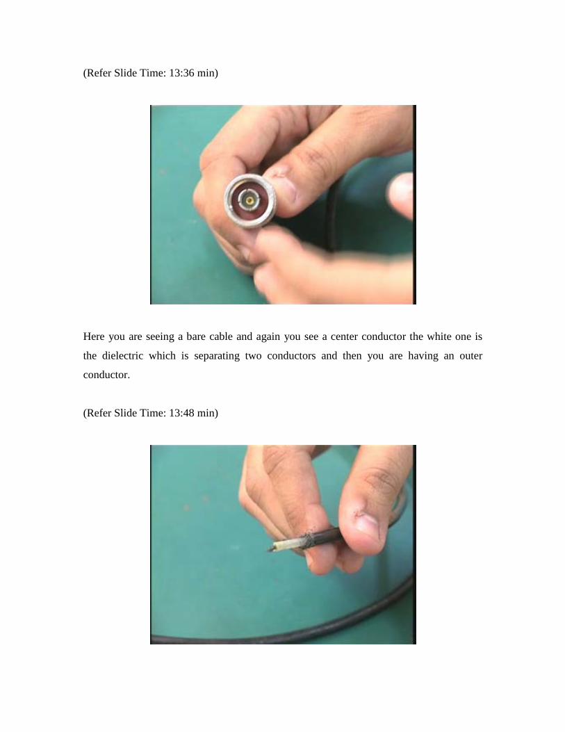
(Refer Slide Time: 13:36 min)
Here you are seeing a bare cable and again you see a center conductor the white one is
the dielectric which is separating two conductors and then you are having an outer
conductor.
(Refer Slide Time: 13:48 min)
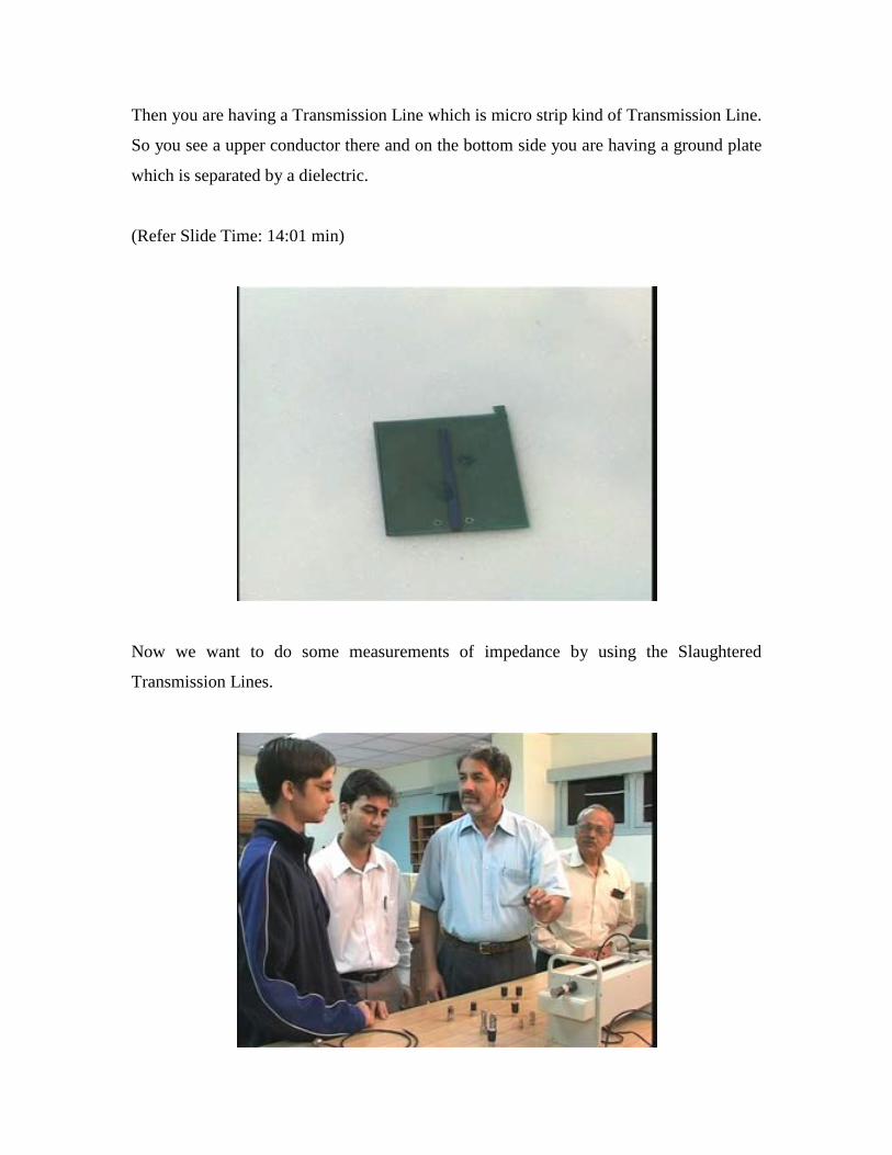
Then you are having a Transmission Line which is micro strip kind of Transmission Line.
So you see a upper conductor there and on the bottom side you are having a ground plate
which is separated by a dielectric.
(Refer Slide Time: 14:01 min)
Now we want to do some measurements of impedance by using the Slaughtered
Transmission Lines.

So here we have a set up for making measurements of VSWR reflection coefficient and
measuring the unknown impedances. What you see here on the table are the different
impedances which are kept there and a setup which called a Slaughtered Transmission
Line.
This is a fifty ohm termination which is open termination.
This is twenty five ohm termination.
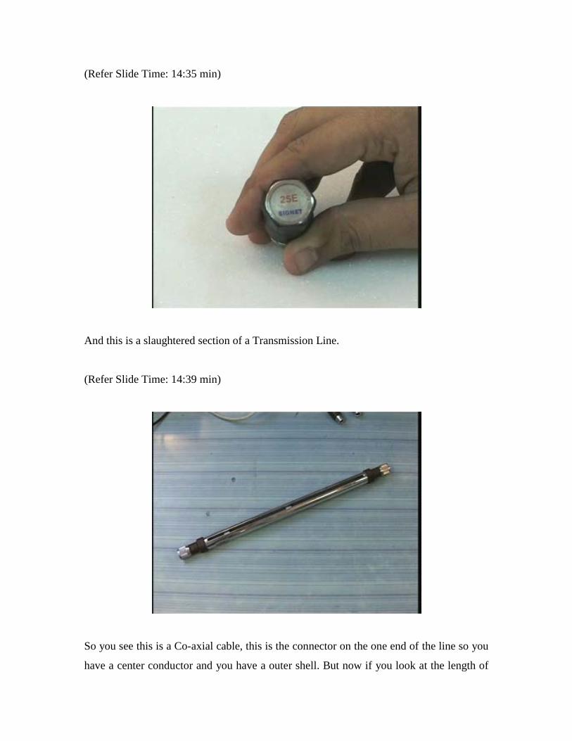
(Refer Slide Time: 14:35 min)
And this is a slaughtered section of a Transmission Line.
(Refer Slide Time: 14:39 min)
So you see this is a Co-axial cable, this is the connector on the one end of the line so you
have a center conductor and you have a outer shell. But now if you look at the length of

the section of the Transmission Line there is a cut which is along the length of this
section in which a voltage probe can be moved and we can measure the voltage along the
Transmission Line.
Here is the set up for measuring the voltage along the length of the Transmission Line
when it is terminated with different impedances.
(Refer Slide Time: 15:05 min)
Here what you are seeing is the voltage probe which is moving with the help of a motor
along the length of the Transmission Line. The voltage is sensed and it is given to the
computer so the computer registers the location of the probe and the voltage measured at
that location. Then computer uses this information to get a plot called the voltage
standing wave pattern which is nothing but the variation of magnitude of voltage along
the length of the Transmission Line when it is terminated in a load.
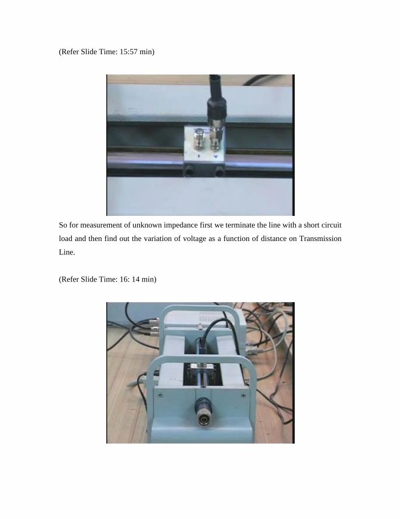
(Refer Slide Time: 15:57 min)
So for measurement of unknown impedance first we terminate the line with a short circuit
load and then find out the variation of voltage as a function of distance on Transmission
Line.
(Refer Slide Time: 16: 14 min)
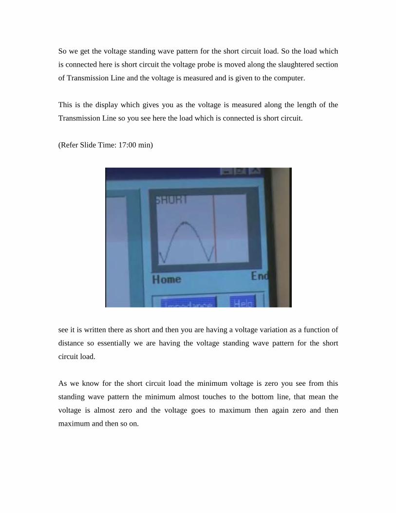
So we get the voltage standing wave pattern for the short circuit load. So the load which
is connected here is short circuit the voltage probe is moved along the slaughtered section
of Transmission Line and the voltage is measured and is given to the computer.
This is the display which gives you as the voltage is measured along the length of the
Transmission Line so you see here the load which is connected is short circuit.
(Refer Slide Time: 17:00 min)
see it is written there as short and then you are having a voltage variation as a function of
distance so essentially we are having the voltage standing wave pattern for the short
circuit load.
As we know for the short circuit load the minimum voltage is zero you see from this
standing wave pattern the minimum almost touches to the bottom line, that mean the
voltage is almost zero and the voltage goes to maximum then again zero and then
maximum and then so on.

Now the same data is displayed on a bigger screen so you can see that voltage pattern
which we were seen in the small window now essentially is available on the full screen.
(Refer Slide Time: 18:00 min)
So this is the voltage standing wave pattern for the short circuit load the blue line gives
you the location of the voltage minimum and the red line gives you the location of the
voltage maximum.
Now let us replace the short circuit load by another load and again measure the voltage
along the length of the Transmission Line.
As you can see the voltage standing wave pattern for this load is in blue the standing
wave pattern for short circuit load is in red and as you can see very clearly that the
minima of the short circuit coincides with maxima of this load also the voltage minimum
is zero that means this load is nothing but the open circuit load.
(Refer Slide Time: 20:18 min)
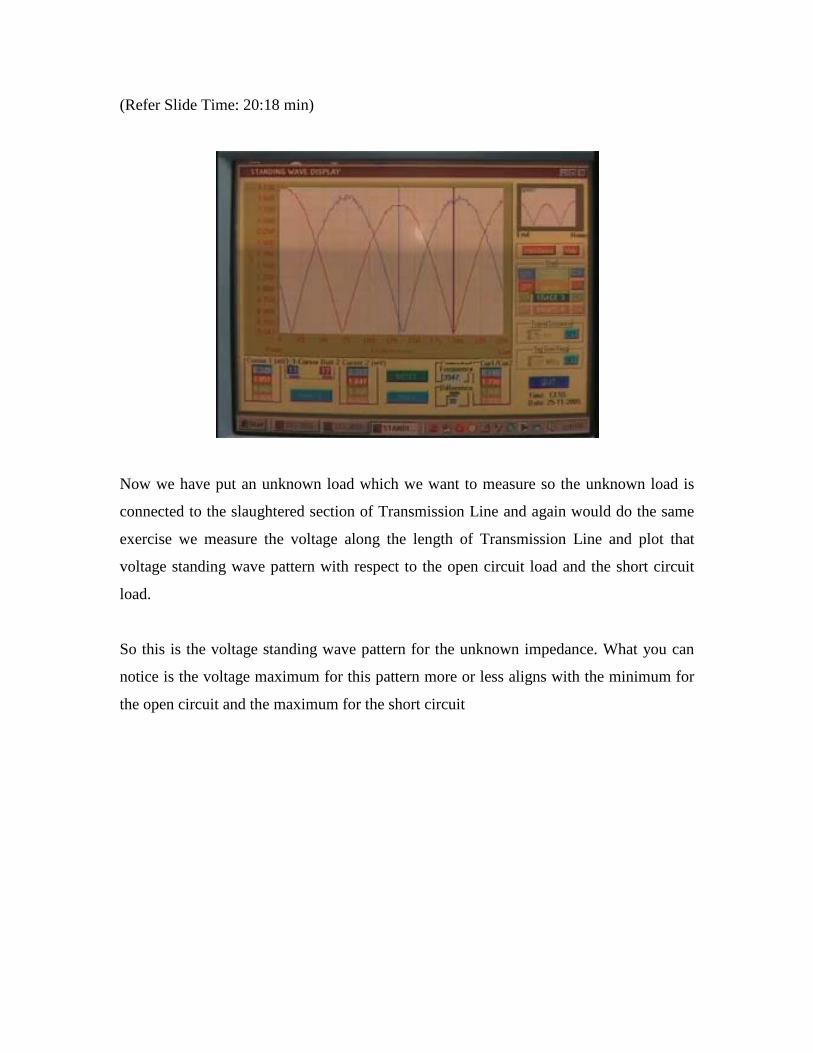
Now we have put an unknown load which we want to measure so the unknown load is
connected to the slaughtered section of Transmission Line and again would do the same
exercise we measure the voltage along the length of Transmission Line and plot that
voltage standing wave pattern with respect to the open circuit load and the short circuit
load.
So this is the voltage standing wave pattern for the unknown impedance. What you can
notice is the voltage maximum for this pattern more or less aligns with the minimum for
the open circuit and the maximum for the short circuit

(Refer Slide Time: 21:30 min)
That means this impedance is almost resistive impedance and since the maxima of this
pattern aligns with the maxima of the short circuit the impedance value is less than the
characteristic impedance.
Let us say one more load and get the standing wave pattern for this load. Then now you
are having this new data which we have got for the voltage maxima or the voltage
minima do not coincide with voltage maxima or voltage minima or by the short circuit or
by the open circuit impedance. Then in general this a general load and then knowing the
VSWR and the location of the voltage maxima or minima we can find the unknown
impedance connected to the Transmission Line.
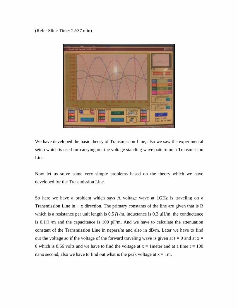
(Refer Slide Time: 22:37 min)
We have developed the basic theory of Transmission Line, also we saw the experimental
setup which is used for carrying out the voltage standing wave pattern on a Transmission
Line.
Now let us solve some very simple problems based on the theory which we have
developed for the Transmission Line.
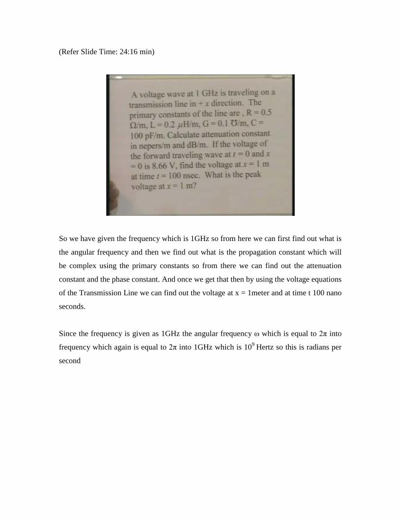
So here we have a problem which says A voltage wave at 1GHz is traveling on a
Transmission Line in + x direction. The primary constants of the line are given that is R
which is a resistance per unit length is 0.5Ω /m, inductance is 0.2 μH/m, the conductance
is 0.1 /m and the capacitance is 100 pF/m. And we have to calculate the attenuation
constant of the Transmission Line in nepers/m and also in dB/m. Later we have to find
out the voltage so if the voltage of the forward traveling wave is given at t = 0 and at x =
0 which is 8.66 volts and we have to find the voltage at x = 1meter and at a time t = 100
nano second, also we have to find out what is the peak voltage at x = 1m.
(Refer Slide Time: 24:16 min)
So we have given the frequency which is 1GHz so from here we can first find out what is
the angular frequency and then we find out what is the propagation constant which will
be complex using the primary constants so from there we can find out the attenuation
constant and the phase constant. And once we get that then by using the voltage equations
of the Transmission Line we can find out the voltage at x = 1meter and at time t 100 nano
seconds.
Since the frequency is given as 1GHz the angular frequency ω which is equal to 2π into
frequency which again is equal to 2π into 1GHz which is 109 Hertz so this is radians per
second

(Refer Slide Time: 25:30 min)
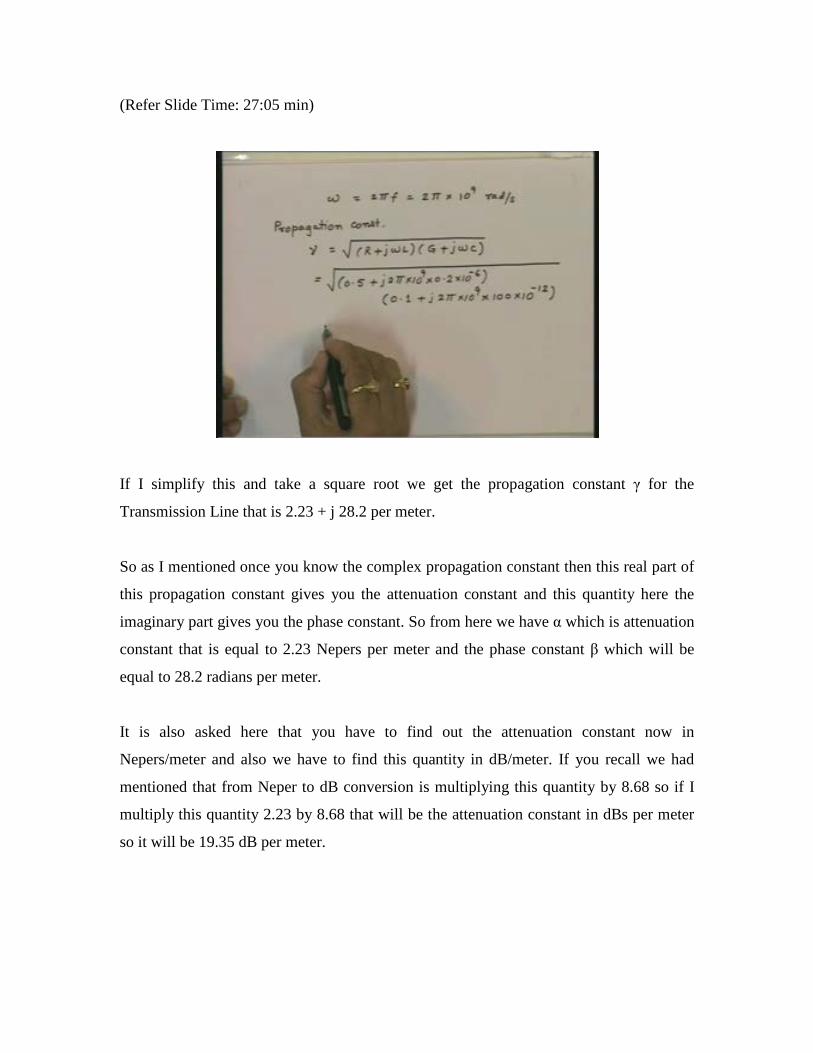
Then we can find out the propagation constant on Transmission Line so we get
propagation constant γ which is equal to square root of ( )( )R j L G j Cω ω+ + and now
we can substitute the value of R, G, L and C so we can write here as this is equal to
square root of 0.5Ω /m that is the value of R plus j2π into 109 which is the angular
frequency ω into L which is 0.2 μH/m into 10-6 multiplied by (G + jωC) so G which is
0.1 /m plus j2π into 109 and C which is 100 pF/m so this is hundred into 10-12.
(Refer Slide Time: 27:05 min)
If I simplify this and take a square root we get the propagation constant γ for the
Transmission Line that is 2.23 + j 28.2 per meter.
So as I mentioned once you know the complex propagation constant then this real part of
this propagation constant gives you the attenuation constant and this quantity here the
imaginary part gives you the phase constant. So from here we have α which is attenuation
constant that is equal to 2.23 Nepers per meter and the phase constant β which will be
equal to 28.2 radians per meter.
It is also asked here that you have to find out the attenuation constant now in
Nepers/meter and also we have to find this quantity in dB/meter. If you recall we had
mentioned that from Neper to dB conversion is multiplying this quantity by 8.68 so if I
multiply this quantity 2.23 by 8.68 that will be the attenuation constant in dBs per meter
so it will be 19.35 dB per meter.

(Refer Slide Time: 28:56 min)
So we have completed the first part of the problem where you have to find out the
attenuation constant on the Transmission Line in nepers per meter and dB per meter.
Now in the second part we now have to find out the voltage at this location that is x = 1m
and at time t = 100 nano second if the initial voltage is given at t = 0 second and x = 0
meters. so now we can use the voltage equation first you find out the quantity which is
the amplitude of the forward traveling wave so by using the initial condition essentially
we calculate the arbitrary constant V+ and then we can find out the voltage at any location
on Transmission Line.
So if I write down the instantaneous voltage at any point on Transmission Line v(t) which
will be nothing but real part of V+ e-αx ej(ωt – βx).

(Refer Slide Time: 30:29 min)
Saying that this quantity V+ in general is a complex quantity and if you write down V+ as
the magnitude of V+ and some initial phase which is jφ . Then this quantity v(t) which is
the real part of this expression can be written as |V+| e-αx and e to the power ejφ will
combine with this so real part of that will be nothing but cos(ωt - βx + φ ).
(Refer Slide Time: 31:19 min)
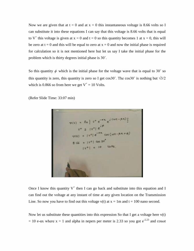
Now we are given that at t = 0 and at x = 0 this instantaneous voltage is 8.66 volts so I
can substitute it into these equations I can say that this voltage is 8.66 volts that is equal
to V+ this voltage is given at x = 0 and t = 0 so this quantity becomes 1 at x = 0, this will
be zero at t = 0 and this will be equal to zero at x = 0 and now the initial phase is required
for calculation so it is not mentioned here but let us say I take the initial phase for the
problem which is thirty degrees initial phase is 30˚.
So this quantity φ which is the initial phase for the voltage wave that is equal to 30˚ so
this quantity is zero, this quantity is zero so I get cos30˚. The cos30˚ is nothing but √3/2
which is 0.866 so from here we get V+ = 10 Volts.
(Refer Slide Time: 33:07 min)
Once I know this quantity V+ then I can go back and substitute into this equation and I
can find out the voltage at any instant of time at any given location on the Transmission
Line. So now you have to find out this voltage v(t) at x = 1m and t = 100 nano second.
Now let us substitute these quantities into this expression So that I get a voltage here v(t)
= 10 e-αx where x = 1 and alpha in nepers per meter is 2.33 so you got e-2.23 and cosωt

which is 2π into 109 into t which is hundred nano second so this is hundred into 10-9
minus βx and as we have seen β for this Transmission Line is 28.2 radians per meter so I
get 28.2 into 1 at x = 1 plus this quantity φ initial phase which is equal to 30˚ so that is
π/6.
If I simplify this then I will get the voltage at x = 1m, at time t = 100 nano seconds which
will be equal to -0.88 Volts.
(Refer Slide Time: 35:36 min)
It is also asked to find out the peak voltage at this location that is x = 1m so if I go in to
this expression the cosine term essentially tells you how the signal is varying as a
function of time at given location x = 1m. This quantity is nothing but the amplitude of
the voltage at that location x = 1m.
So the peak voltage vpeak at x = 1m will be equal to 10 e-2.23 which is nothing but one
1.075 volts.

(Refer Slide Time: 36:42 min)
So this is one of simplest problem we can think on Transmission Line where the
Transmission Line primary constants are given, the voltage at some instant of time and
some location of Transmission Line is given and we are asked to find out the voltage at
some other location and some other instant of time on the Transmission Line.
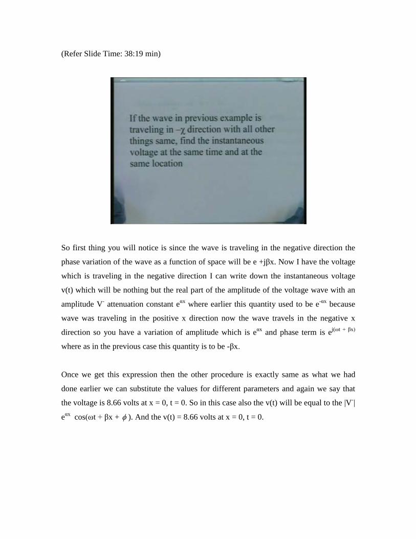
Now one can ask that if I have same problem if the wave was moving in the negative x
direction instead of wave moving in the positive x direction and if the initial conditions
were same that means at t = 0 and x = 0 the voltage was 8.66 volts then how the things
would change. so we are still want to find out the voltage at this location x = 1m this is
time t = 100 nano second only thing now we say is that the direction of the wave is
reversed that means now the wave travels in the negative x direction.
so what we are saying is if the wave in the previous example the example which we saw
just now is traveling in negative x direction with all other things same find the
instantaneous voltage at the same time and at the same location that means find the
voltage at x = 1m and t = 100 nano second.
(Refer Slide Time: 38:19 min)
So first thing you will notice is since the wave is traveling in the negative direction the
phase variation of the wave as a function of space will be e +jβx. Now I have the voltage
which is traveling in the negative direction I can write down the instantaneous voltage
v(t) which will be nothing but the real part of the amplitude of the voltage wave with an
amplitude V- attenuation constant eαx where earlier this quantity used to be e-αx because
wave was traveling in the positive x direction now the wave travels in the negative x
direction so you have a variation of amplitude which is eαx and phase term is ej(ωt + βx)
where as in the previous case this quantity is to be -βx.
Once we get this expression then the other procedure is exactly same as what we had
done earlier we can substitute the values for different parameters and again we say that
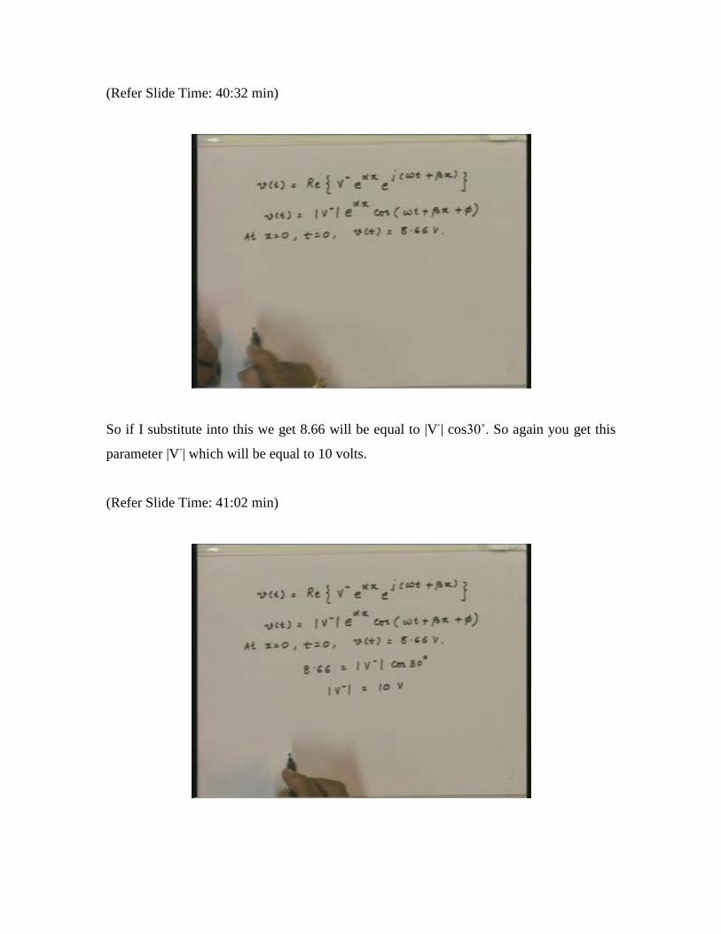
the voltage is 8.66 volts at x = 0, t = 0. So in this case also the v(t) will be equal to the |V-|
eαx cos(ωt + βx + φ ). And the v(t) = 8.66 volts at x = 0, t = 0.
(Refer Slide Time: 40:32 min)
So if I substitute into this we get 8.66 will be equal to |V-| cos30˚. So again you get this
parameter |V-| which will be equal to 10 volts.
(Refer Slide Time: 41:02 min)

Now if I substitute this quantity |V-| = 10 volts in this expression then I get the voltage at t
= 100 nano second and x = 1m will be v(t) = 10 e2.23 cos of the whole thing the ωt which
we have already calculated earlier plus βx plus the angle φ which is equal to 30˚ which is
π/6. If I simplify this then we get the voltage which is minus -83.77 volts.
(Refer Slide Time: 42:17 min)
So what you notice here now is that if I look at the situation that this is my Transmission
Line and this was the location which is let us say x = 0, this is the location which is x =
m. If the wave travels in the forward direction then the wave will attenuate in the
direction of propagation so initially you had certain value of the voltage which is 8.66.
But since the wave is attenuating in the forward direction you have the amplitude
variation of the wave which looks like this so 8.66 becomes something which we
calculated earlier 0.88 volts so this quantity was 8.66 volts and this at 0.88 volts. So this
would be the variation for the forward wave.
But to have the same amplitude here 8.66 and if the wave is traveling backwards then the
attenuation is at the direction of wave propagation which is in this direction so for the
same value here 8.66 volts now the amplitude variation would look something like that

and that was precisely is happening. Now the voltage amplitude which we get for this
wave is which we saw is -83.77 volts so this problem clearly demonstrates that the
direction of the wave propagation is very important for the same location on
Transmission Line and same time the voltage values will be quite different depending
upon whether the wave was traveling in one direction or other.
(Refer Slide Time: 44:32 min)
So this problem essentially gives a feel for how the voltages vary on a Transmission Line
and how important is this aspect of the direction of wave propagation on the
Transmission Line.
Now let us look at a problem of low-loss transmission line. In practice we always have a
resistance in Transmission Line though you may always use a very high quality dielectric
material so the conductance per unit length of Transmission Line could be very small but
the resistance is not really very small for a practical Transmission Line so invariably a
question is asked that what is the acceptable value of the resistance per unit length of
Transmission Line so the line can be used or it can treated as the low-loss transmission
line.
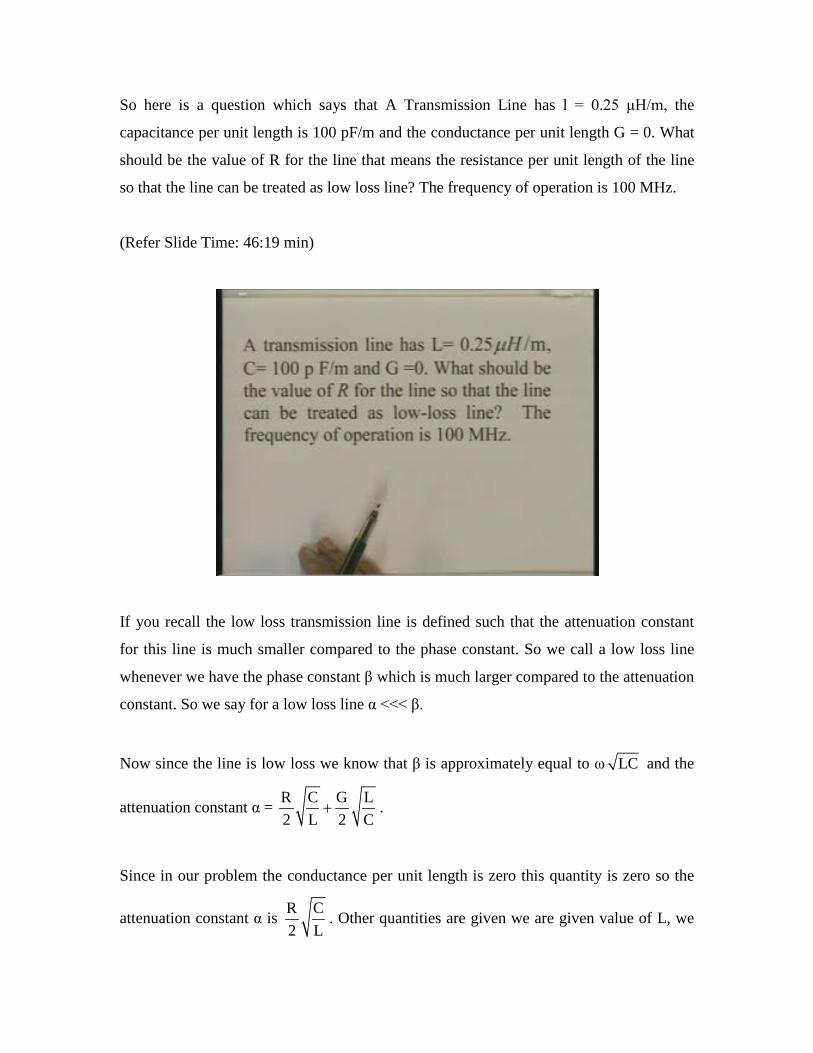
So here is a question which says that A Transmission Line has l = 0.25 μH/m, the
capacitance per unit length is 100 pF/m and the conductance per unit length G = 0. What
should be the value of R for the line that means the resistance per unit length of the line
so that the line can be treated as low loss line? The frequency of operation is 100 MHz.
(Refer Slide Time: 46:19 min)
If you recall the low loss transmission line is defined such that the attenuation constant
for this line is much smaller compared to the phase constant. So we call a low loss line
whenever we have the phase constant β which is much larger compared to the attenuation
constant. So we say for a low loss line α <<< β.
Now since the line is low loss we know that β is approximately equal to ω LC and the
attenuation constant α = R C G L2 L 2 C
+ .
Since in our problem the conductance per unit length is zero this quantity is zero so the
attenuation constant α is R C2 L
. Other quantities are given we are given value of L, we
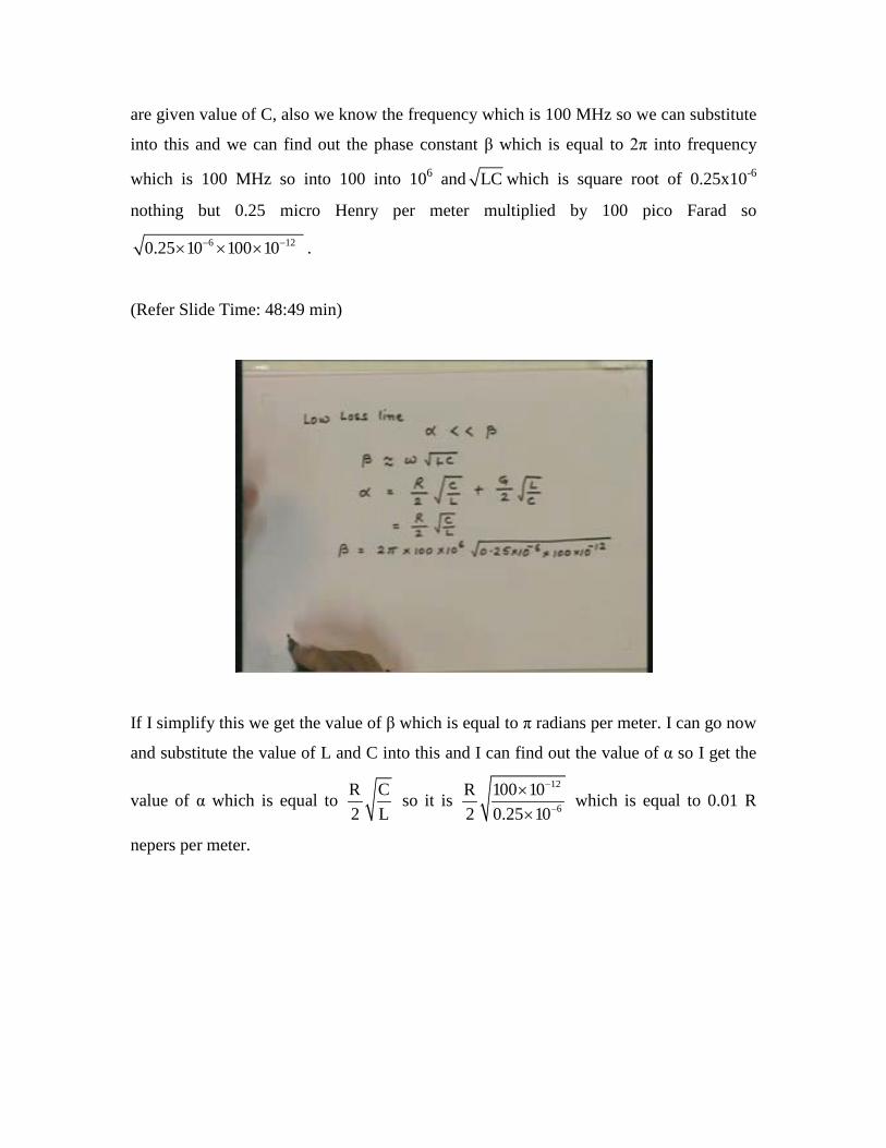
are given value of C, also we know the frequency which is 100 MHz so we can substitute
into this and we can find out the phase constant β which is equal to 2π into frequency
which is 100 MHz so into 100 into 106 and LC which is square root of 0.25x10⁻⁶
nothing but 0.25 micro Henry per meter multiplied by 100 pico Farad so
6 120.25 10 100 10 − −× × × .
(Refer Slide Time: 48:49 min)
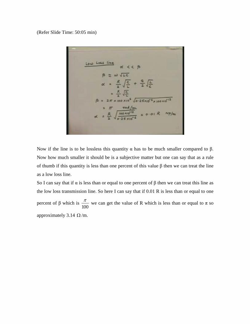
If I simplify this we get the value of β which is equal to π radians per meter. I can go now
and substitute the value of L and C into this and I can find out the value of α so I get the
value of α which is equal to R C2 L
so it is 12
6
R 100 102 0.25 10
−
−
××
which is equal to 0.01 R
nepers per meter.
(Refer Slide Time: 50:05 min)
Now if the line is to be lossless this quantity α has to be much smaller compared to β.
Now how much smaller it should be is a subjective matter but one can say that as a rule
of thumb if this quantity is less than one percent of this value β then we can treat the line
as a low loss line.
So I can say that if α is less than or equal to one percent of β then we can treat this line as
the low loss transmission line. So here I can say that if 0.01 R is less than or equal to one
percent of β which is 100π we can get the value of R which is less than or equal to π so
approximately 3.14 Ω /m.

(Refer Slide Time: 51:45 min)
So for this Transmission Line if I take the resistance less than about 3 Ω /m then this line
can be treated as a low loss transmission line.
If the value of resistance exceeds this value then slowly the line will become a lossy
transmission line and when the value of the resistance becomes comparable to β then we
will get the variation or the performance of the line which will be extremely lossy
transmission line.
So in this session essentially we first saw how to identify the load which is terminating
the line so just qualitatively looking at the voltage standing wave patterns one can
identify the type of load which is connected to the Transmission Line. Then we went to
the laboratory and we saw the experimental setups which are used for measurement of
VSWR or Voltage Standing Wave Patterns on Transmission Line. And then later we
solved some very simple problems based on the voltage equations which we have derive
for the Transmission Line.

In the next session we will go to the applications of the Transmission Lines that means
having understood the behavior of voltage and current on Transmission Lines, how do we
make use of sections of Transmission Lines in realizing various circuit elements in the
high frequency circuits.
In the next session essentially we discuss the applications of Transmission Lines.
Thank you.