stat modeling and time series

1

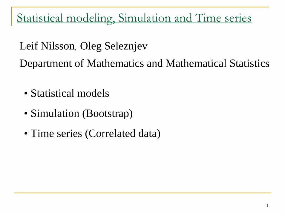
Statistical modeling, Simulation and Time series

Leif Nilsson, Oleg SeleznjevDepartment of Mathematics and Mathematical Statistics

• Statistical models

• Simulation (Bootstrap)

• Time series (Correlated data)

2

Statistical modeling

• How do humans react on a specific drug. • How do the sizes of piston rings behave in a production process.• How do processing conditions, e.g. reaction time, reaction

temperature, and type of catalyst, affect the yield of a chemical reaction.

• When the government plans for the future they need good prediction models for e.g. the Gross National Product (GNP).

By making observations and using statistical methods we can handle these kind of situations.

In many cases it is very hard to mathematically model a situation without observations.

3


Sometimes we know the model apart from one or more parameters.These parameter can then be estimated from data.

Natural questions are• what accuracy and precision do the estimates have?• how accurate will a prediction be?

These questions can also be handled with statistical methods.

4


When we have a mathematical model for a situation it can be of importance to verify how well this model agree with the reality.This can be done by comparing observations with the model (or simulated observations from the model).Here can statistical methods be useful.

Sometimes it is more or less impossible to make observations,e.g. the amounts of large insurance losses, extreme floods, …The extreme value theory can be used to model such situations.

5


Consider the flow of current in a thin copper wire. A mechanistic model is Ohm’s law:

current = voltage/resistance (I=E/R)If we measure this more than once, perhaps at different days, the observed current could differ slightly because of small changes or variations in factors that are not completely controlled (temperature, measuring technique, …).A more realistic (statistical) model for the observed current might be

I = E/R + ε = μ + ε,where the term ε includes the effect of all of unmodeled sources of variability that effects this system.

6


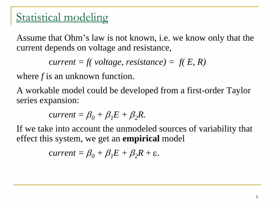
Assume that Ohm’s law is not known, i.e. we know only that the current depends on voltage and resistance,

current = f( voltage, resistance) = f( E, R)where f is an unknown function.A workable model could be developed from a first-order Taylor series expansion:

current = β0 + β1E + β2R.If we take into account the unmodeled sources of variability that effect this system, we get an empirical model

current = β0 + β1E + β2R + ε.

7


What is a reasonable model for ε.

Often we believe that there exists a large number of small effects acting additively and independently on the measurements, i.e. ε is a sum of these small effects.

The Central Limit Theorem (CLT) tells us that the distribution of a sum of a large number of independent variables is approximately normal.

In that case, ε is assumed to be normally distributed with expected value 0 and standard deviation σ, ε ∈N(0, ) .

This means that the measurements are also normally distributed with standard deviation σ.

2σ

8


Sometimes the small effects are acting multiplicatively and independently on the measurements, i.e. ε is a product of these small effects.

In that case, it is reasonable to believe that the measurements(and ε) are log-normally distributed, that is log(measurement) and (log(ε)) is normally distributed.

Depending on the situation, one has to investigate what distribution the observations follow.

There exists a large amount of distributions: binomial, Poisson, uniform, beta, Cauchy, gamma, lognormal, normal, Weibull,….

9


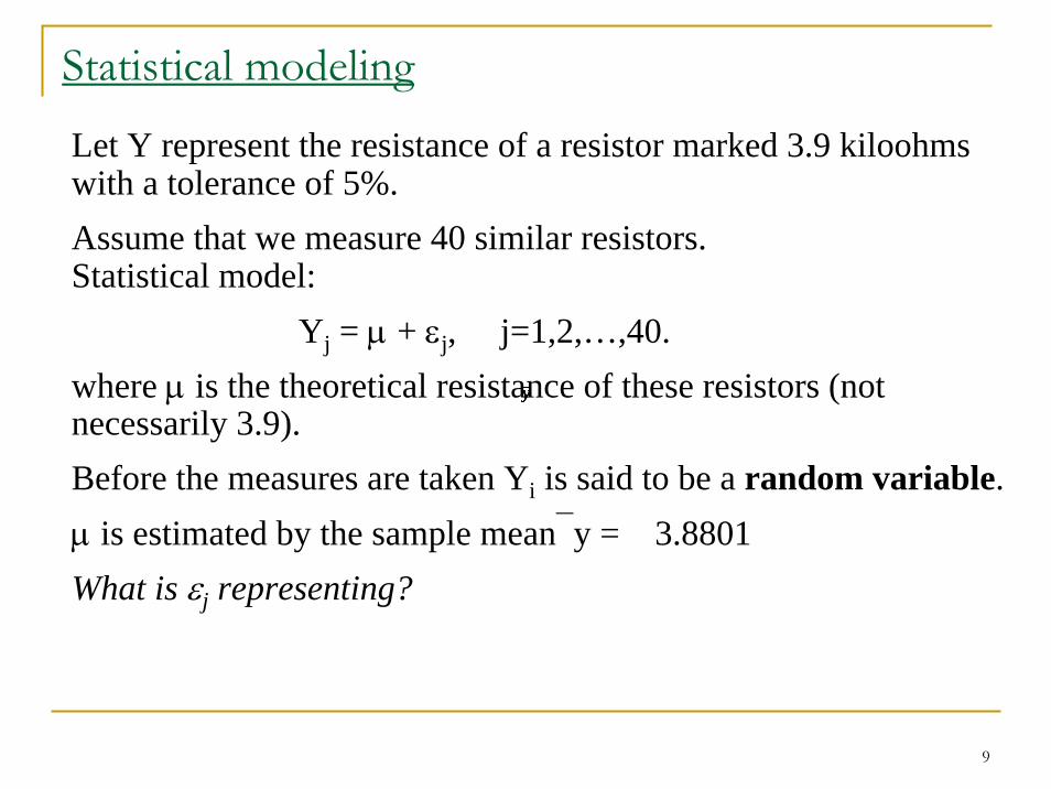
Let Y represent the resistance of a resistor marked 3.9 kiloohmswith a tolerance of 5%.Assume that we measure 40 similar resistors. Statistical model:

Yj = μ + εj, j=1,2,…,40.where μ is the theoretical resistance of these resistors (not necessarily 3.9).Before the measures are taken Yi is said to be a random variable.μ is estimated by the sample mean⎯y = 3.8801What is εj representing?

yyyyyy

10


The measurements are varying.

A theoretical standard deviation σ exists and

is estimated with the sample standard deviation: s = 0.0030

If data is normally distributed, the 95% of the measurements should roughly lie within the interval

⎯y ± 1.96*s = 3.8801 ± 0.0059 = ( 3.8742, 3.8860).

2 2

1( ) / ( 1)

n

ii

s y y n=

= − −∑

11


We can test the hypothesis H0: μ =3.9 (alternative H1: μ ≠ 3.9)

by comparing⎯y with μ = 3.9.

The estimate of the standard deviation of ⎯y is s/√40 = 0.00047 Since the data consist of 40 measurements, the sample mean is (approximately) normally distributed with mean μ and standard deviation σ/√40 (CLT).A 95% confidence interval is calculated as

⎯y ± 1.96*s /√40 = 3.8801 ± 0.0009359 = (3.8792, 3.8810).

We can reject H0: μ =3.9.

How do we interpret the interval?

12


We can also test the hypothesis H0: μ =3.9 (H1: μ ≠ 3.9)

by computing p-values.

If the calculated p-value is smaller than the pre-chosen level of significance α

(usually α=0.05, correspond to 95% confidence interval),

The null-hypothesis H0 is rejected. Let us calculate the p-value and confidence interval with Matlab (with Statistics toolbox)Data (resistance):3.883 3.883 3.880 3.875 3.881 3.877 3.880 3.877 3.877 3.881 3.876 3.881 3.881 3.875 3.875 3.880 3.878 3.875 3.884 3.880 3.877 3.883 3.882 3.886 3.877 3.880 3.883 3.884 3.880 3.879 3.880 3.881 3.882 3.879 3.885 3.886 3.879 3.881 3.880 3.881

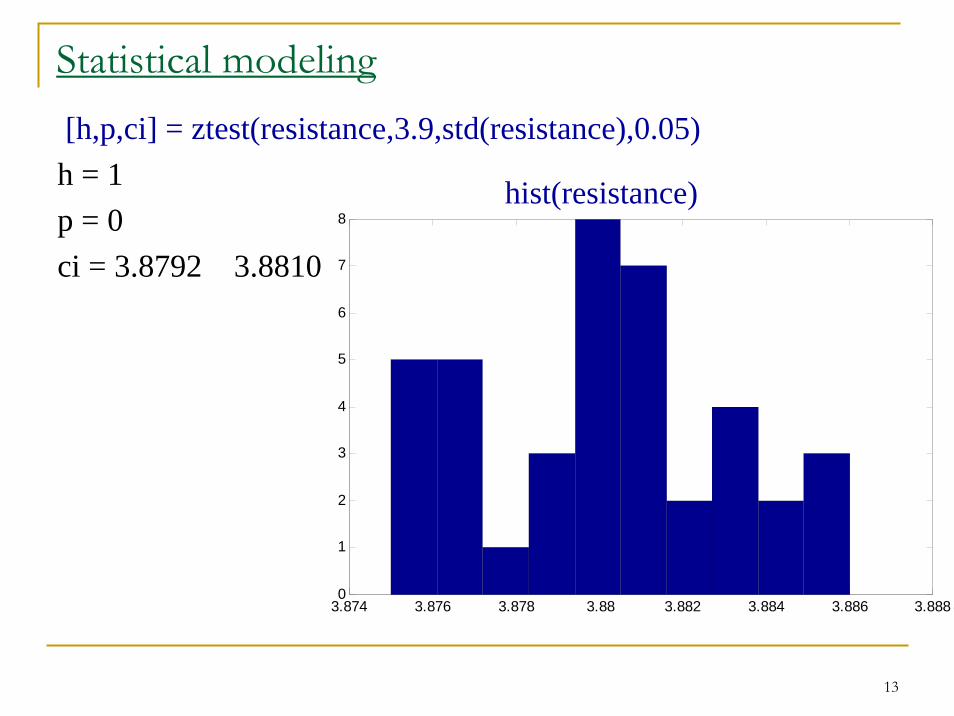
13

Statistical modeling[h,p,ci] = ztest(resistance,3.9,std(resistance),0.05)h = 1p = 0ci = 3.8792 3.8810

3.874 3.876 3.878 3.88 3.882 3.884 3.886 3.8880

1

2

3

4

5

6

7

8hist(resistance)

14

Bootstrap

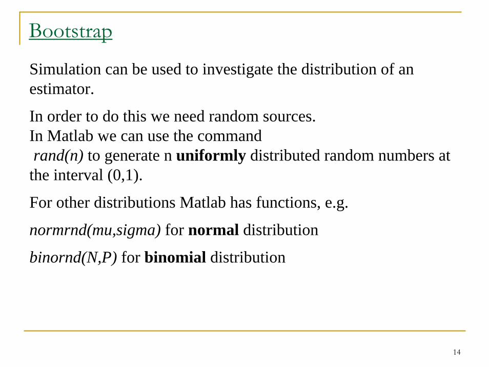
Simulation can be used to investigate the distribution of an estimator.

In order to do this we need random sources. In Matlab we can use the commandrand(n) to generate n uniformly distributed random numbers at the interval (0,1).

For other distributions Matlab has functions, e.g.

normrnd(mu,sigma) for normal distribution

binornd(N,P) for binomial distribution

15

Bootstrap

The term “Bootstrap” (Efron, 1979 ) is an allusion to the expression "pulling oneself up by one's bootstraps” (doing the impossible).

Traditional statistical methods are either

based upon the large sample theory or

prior beliefs or

inferences based upon small samples.

In most situations, bootstrap usually produces more accurate andreliable results than the traditional methods.

Bootstrap is especially useful when complicated estimators are to be analyze.

16

Bootstrap

Non-parametric bootstrap:

Assume that we are interested in an estimate of the observed sample (y1, y2, …, yn): e.g ⎯y, s, median, s /⎯y, ….

Construct artificial samples by resampling with replacement from the observed sample.

These artificial samples are regarded as new observed samples.

Calculate the estimate with the resampled data: e.g ⎯y*, s*, …

By doing this many times (say B times) we receive B estimates

that will behave approximately as the true estimator will behave.

Let us illustrate this in Matlab.

) y..., , y,(y *n

*2

*1

)y ..., ,y ,y( *B

*2

*1

17

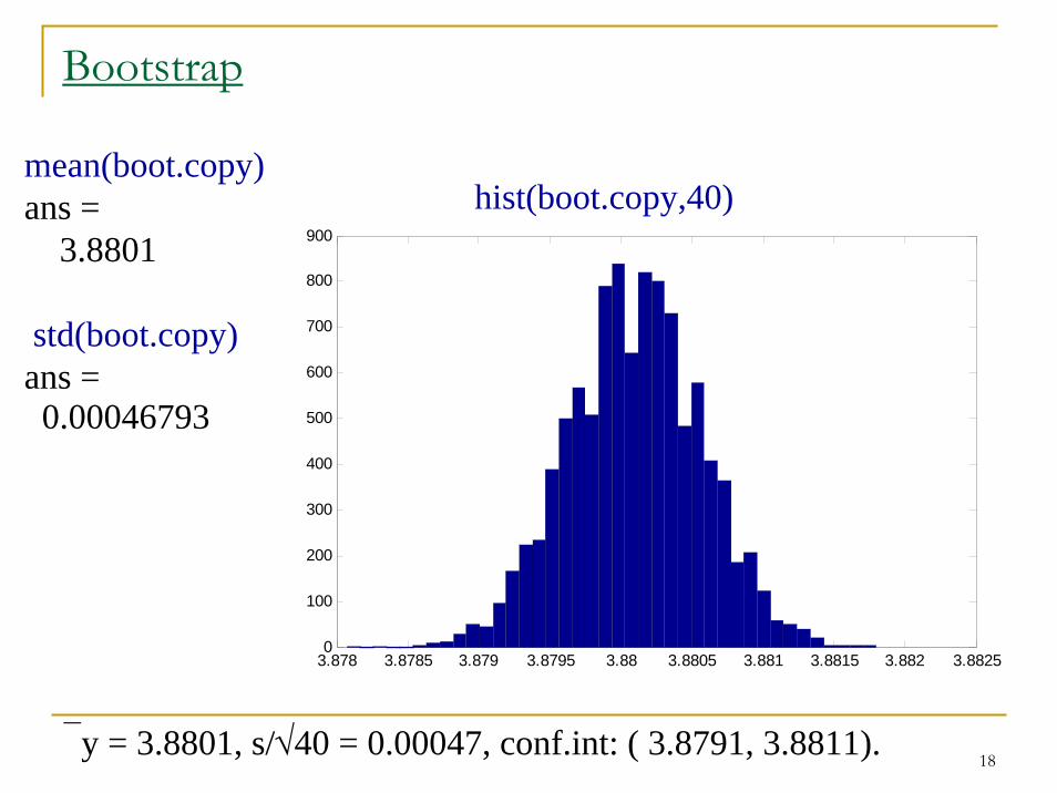
BootstrapData (resistance): 3.883 3.883 3.880 3.875 3.881 3.877 3.880 3.877 3.877 3.881 3.876 3.881 3.881 3.875 3.875 3.880 3.878 3.875 3.884 3.880 3.877 3.883 3.882 3.886 3.877 3.880 3.883 3.884 3.880 3.879 3.880 3.881 3.882 3.879 3.885 3.886 3.879 3.881 3.880 3.881

CLT tells us that the sample mean will be approximately normallydistributed with mean μ and standard deviation σ/√40.

B = 10000;for i = 1:Bsample=randsample(resistance,40,true);boot.copy(i)=mean(sample);end

or shorterboot.copy = bootstrp(B, 'mean', resistance);

With replacement

18

Bootstrap

⎯y = 3.8801, s/√40 = 0.00047, conf.int: ( 3.8791, 3.8811).

mean(boot.copy)ans =

3.8801

std(boot.copy)ans =0.00046793

hist(boot.copy,40)

3.878 3.8785 3.879 3.8795 3.88 3.8805 3.881 3.8815 3.882 3.88250

100

200

300

400

500

600

700

800

900

19

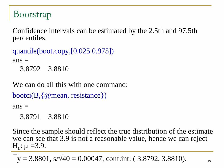
BootstrapConfidence intervals can be estimated by the 2.5th and 97.5th percentiles.

quantile(boot.copy,[0.025 0.975])ans =

3.8792 3.8810

We can do all this with one command:bootci(B,{@mean, resistance})ans =

3.8791 3.8810

Since the sample should reflect the true distribution of the estimate we can see that 3.9 is not a reasonable value, hence we can reject H0: μ =3.9.

⎯y = 3.8801, s/√40 = 0.00047, conf.int: ( 3.8792, 3.8810).

20

Bootstrap

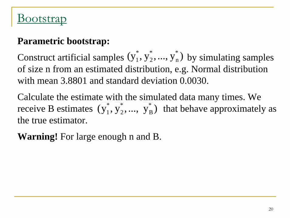
Parametric bootstrap:

Construct artificial samples by simulating samples of size n from an estimated distribution, e.g. Normal distribution with mean 3.8801 and standard deviation 0.0030.

Calculate the estimate with the simulated data many times. We receive B estimates that behave approximately as the true estimator.

Warning! For large enough n and B.

) y..., , y,(y *n

*2

*1

)y ..., ,y ,y( *B

*2

*1

21

BootstrapB=10000mu=mean(resistance);s=std(resistance);

for i = 1:Bsample= normrnd(mu,s,[1,40]);boot.copy(i)=mean(sample);end

mean(boot.copy)ans = 3.8801std(boot.copy)ans = 0.00047556quantile(boot.copy,[0.025 0.975])ans = 3.8792 3.8811

3.878 3.8785 3.879 3.8795 3.88 3.8805 3.881 3.8815 3.882 3.88250

100

200

300

400

500

600

700

22

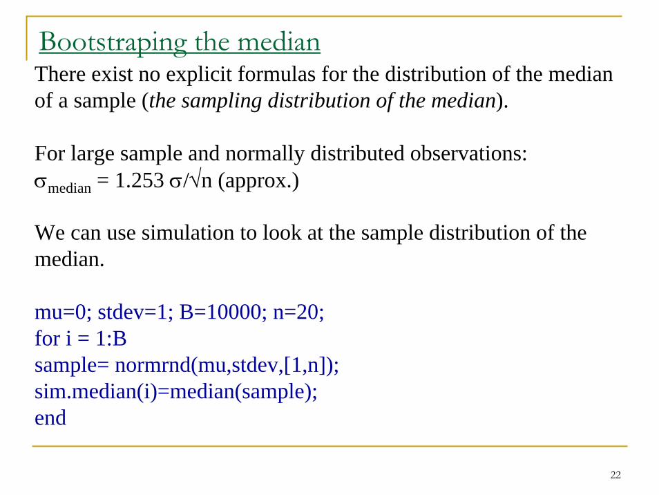
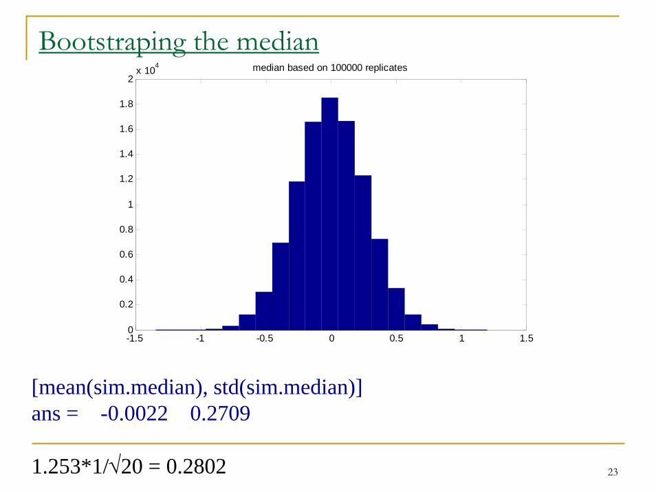
Bootstraping the medianThere exist no explicit formulas for the distribution of the median of a sample (the sampling distribution of the median).

For large sample and normally distributed observations: σmedian = 1.253 σ/√n (approx.)

We can use simulation to look at the sample distribution of the median.

mu=0; stdev=1; B=10000; n=20;for i = 1:Bsample= normrnd(mu,stdev,[1,n]);sim.median(i)=median(sample);end

23

Bootstraping the median

[mean(sim.median), std(sim.median)]ans = -0.0022 0.2709

1.253*1/√20 = 0.2802

-1.5 -1 -0.5 0 0.5 1 1.50

0.2

0.4

0.6

0.8

1

1.2

1.4

1.6

1.8

2x 104 median based on 100000 replicates

24

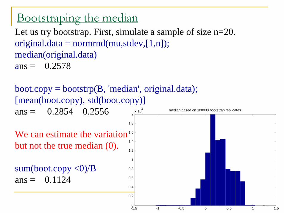
Bootstraping the medianLet us try bootstrap. First, simulate a sample of size n=20.original.data = normrnd(mu,stdev,[1,n]);median(original.data)ans = 0.2578

boot.copy = bootstrp(B, 'median', original.data);[mean(boot.copy), std(boot.copy)]ans = 0.2854 0.2556

We can estimate the variationbut not the true median (0).

sum(boot.copy <0)/Bans = 0.1124

-1.5 -1 -0.5 0 0.5 1 1.50

0.2

0.4

0.6

0.8

1

1.2

1.4

1.6

1.8

2x 10

4 median based on 100000 bootstrap replicates

25

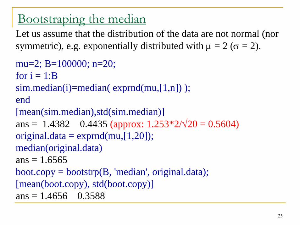
Bootstraping the medianLet us assume that the distribution of the data are not normal (nor symmetric), e.g. exponentially distributed with μ = 2 (σ = 2).

mu=2; B=100000; n=20;for i = 1:Bsim.median(i)=median( exprnd(mu,[1,n]) );end[mean(sim.median),std(sim.median)]ans = 1.4382 0.4435 (approx: 1.253*2/√20 = 0.5604)original.data = exprnd(mu,[1,20]);median(original.data)ans = 1.6565boot.copy = bootstrp(B, 'median', original.data);[mean(boot.copy), std(boot.copy)]ans = 1.4656 0.3588

26

Bootstraping the median

0 0.5 1 1.5 2 2.5 3 3.5 4 4.5 50

0.5

1

1.5

2

2.5x 104 median based on 100000 exp(2) replicates

0 0.5 1 1.5 2 2.5 3 3.5 4 4.5 50

0.5

1

1.5

2

2.5x 104 median based on 100000 bootstrap replicates

True Bootstrap

27

Correlated dataLet X and Y be two dependent random variables.μX = E(X) and μY = E(Y) denote their expected values.The variances are defined as V(X) = E(X - μX)2 and V(X) = E(Y - μY)2.The covariance is defined asCov(X, Y) = E((X - μX) (Y - μY)) = E(XY) - μXμY,and the correlation coefficient as

Corr(X, Y) =

All these measures are in practice usually not known and need tobe estimated from samples (observations).

V(X)V(Y)Y)Cov(X,

28

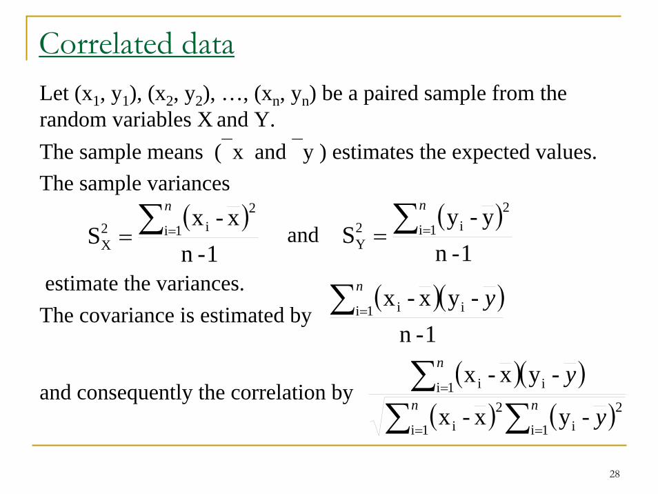
Correlated dataLet (x1, y1), (x2, y2), …, (xn, yn) be a paired sample from the random variables X and Y. The sample means (⎯x and ⎯y ) estimates the expected values.The sample variances

and

estimate the variances.The covariance is estimated by

and consequently the correlation by

( )1-n

x-xS 1i

2i2

X∑ ==

n ( )1-n

y-yS 1i

2i2

Y∑ ==

n

( )( )1-n

-yx-x1i ii∑ =

n y

( )( )( ) ( )∑∑

∑==

=nn

n

y

y

1i2

i1i2

i

1i ii

-yx-x

-yx-x

29

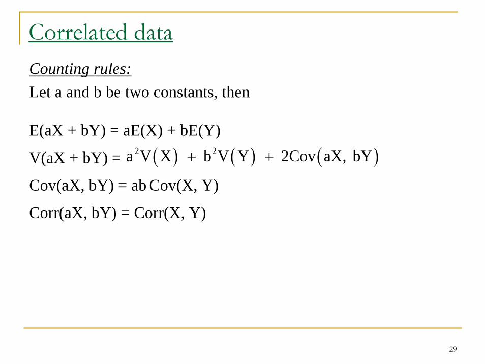
Correlated dataCounting rules:Let a and b be two constants, then

E(aX + bY) = aE(X) + bE(Y)

V(aX + bY) =

Cov(aX, bY) = ab Cov(X, Y)

Corr(aX, bY) = Corr(X, Y)

( ) ( ) ( )2 2a V X b V Y 2Cov aX, bY+ +

30

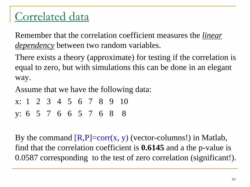
Correlated dataRemember that the correlation coefficient measures the linear dependency between two random variables. There exists a theory (approximate) for testing if the correlation is equal to zero, but with simulations this can be done in an elegant way.Assume that we have the following data:x: 1 2 3 4 5 6 7 8 9 10y: 6 5 7 6 6 5 7 6 8 8

By the command [R,P]=corr(x, y) (vector-columns!) in Matlab, find that the correlation coefficient is 0.6145 and a the p-value is 0.0587 corresponding to the test of zero correlation (significant!).

31

0 1 2 3 4 5 6 7 8 9 10 110

1

2

3

4

5

6

7

8

9

10y vs x

x

yCorrelated data

-1 -0.8 -0.6 -0.4 -0.2 0 0.2 0.4 0.6 0.8 10

100

200

300

400

500

600

700

800

900

-1 -0.8 -0.6 -0.4 -0.2 0 0.2 0.4 0.6 0.8 10

100

200

300

400

500

600

700

800

900

32

BootstrapWe can use bootstrap to analyze the correlation coefficient.Remember that we need to retain the dependency structure, and this is done by pairwise resampling.B=10000;boot.copy=bootstrp(B,'corr',x,y);hist(boot.copy,50)sum(boot.copy < 0)/Bans =

0.0036Notice that this is a p-value for a one sided test

33

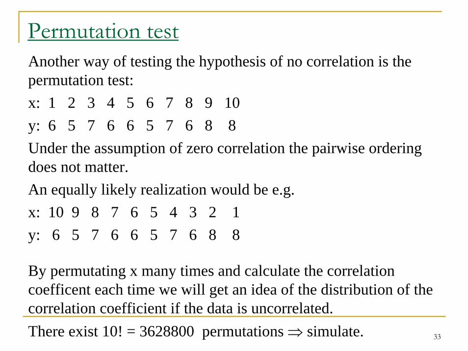
Permutation testAnother way of testing the hypothesis of no correlation is the permutation test:x: 1 2 3 4 5 6 7 8 9 10y: 6 5 7 6 6 5 7 6 8 8Under the assumption of zero correlation the pairwise ordering does not matter.An equally likely realization would be e.g.x: 10 9 8 7 6 5 4 3 2 1y: 6 5 7 6 6 5 7 6 8 8

By permutating x many times and calculate the correlation coefficent each time we will get an idea of the distribution of the correlation coefficient if the data is uncorrelated.There exist 10! = 3628800 permutations ⇒ simulate.

34

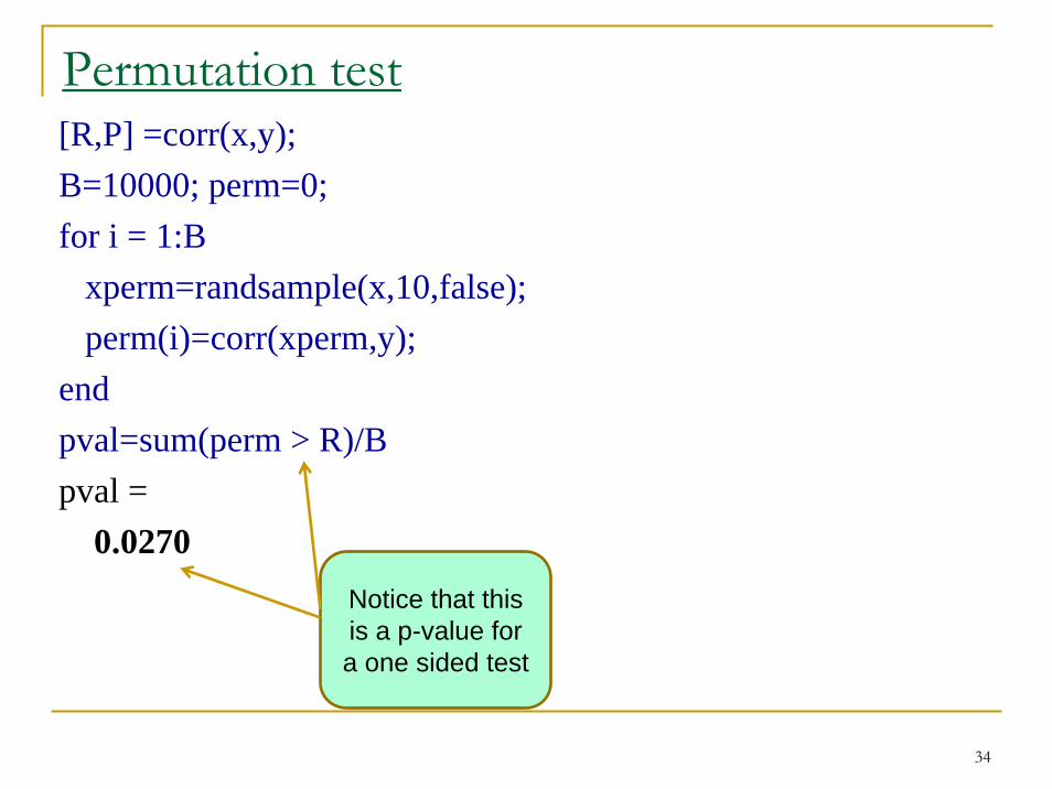
Permutation test[R,P] =corr(x,y);B=10000; perm=0; for i = 1:B

xperm=randsample(x,10,false);perm(i)=corr(xperm,y);

endpval=sum(perm > R)/Bpval =

0.0270Notice that this is a p-value for a one sided test

35

Correlated data

R = 0.6145

-1 -0.8 -0.6 -0.4 -0.2 0 0.2 0.4 0.6 0.8 10

200

400

600

800

1000

1200hist(perm,20)

References

A. M. Zoubir, D. R. Iskander, Bootstrap techniques for signal processing. Cambridge Un Press, 2004A. M. Zoubir, D. R. Iskander, Bootstrap Matlab Toolbox http://www.csp.curtin.edu.au/downloads/bootstrap_toolbox.html

1

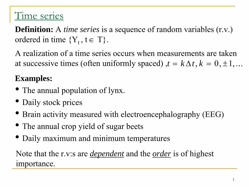
Time seriesDefinition: A time series is a sequence of random variables (r.v.) ordered in time {Yt , t ∈ T}.

A realization of a time series occurs when measurements are taken at successive times (often uniformly spaced) , .

Examples:• The annual population of lynx.• Daily stock prices• Brain activity measured with electroencephalography (EEG)• The annual crop yield of sugar beets• Daily maximum and minimum temperatures

Note that the r.v:s are dependent and the order is of highest importance.

, 0, 1, ...t k t k= Δ = ±

2

Time series

1850 1860 1870 1880 1890 1900 1910 1920 19300

10

20

30

40

50

60

70

80

Time Series Plot of Lynx

Time (seconds)

Time Series/Lynx

Tstool in Matlab

3

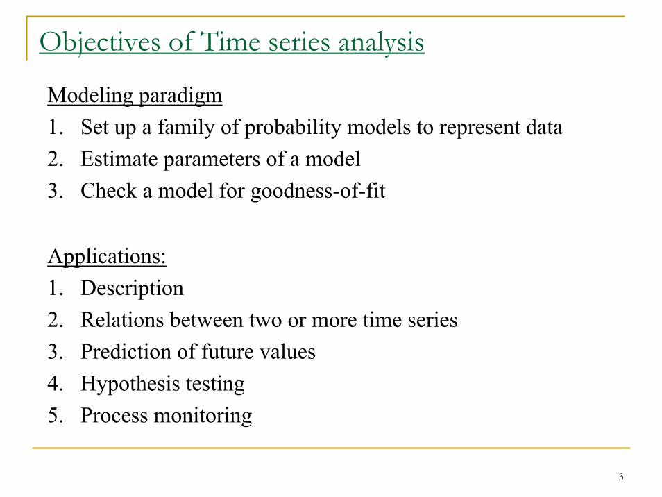
Objectives of Time series analysis

Applications:1. Description2. Relations between two or more time series3. Prediction of future values4. Hypothesis testing5. Process monitoring

Modeling paradigm1. Set up a family of probability models to represent data2. Estimate parameters of a model3. Check a model for goodness-of-fit

4

Time seriesA time series {Yt, t=1,2,…} can contain• a trend Tt (slowly varying)• a long time cyclic influence Zt (e.g. business cycle)• a short time cyclic influence St (e.g. seasonal effect)• an error term (random) εt.

Yt = Tt + Zt + St + εt, t = 1,2,…

In the Lynx data, it seems to be a cyclic behavior and no trend?!

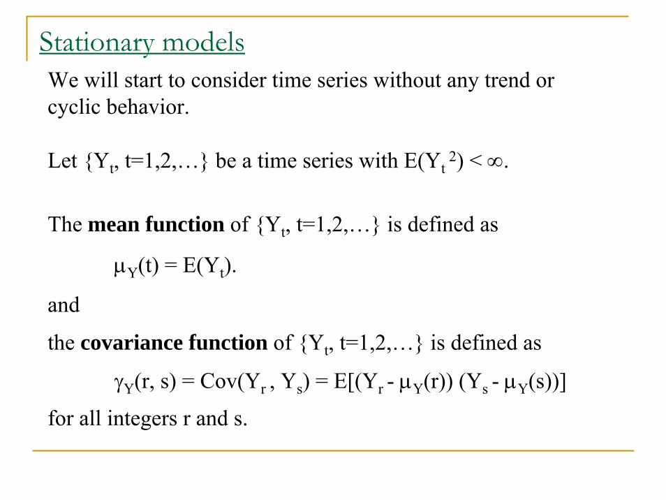
Stationary modelsWe will start to consider time series without any trend or cyclic behavior.

Let {Yt, t=1,2,…} be a time series with E(Yt2) < ∞.

The mean function of {Yt, t=1,2,…} is defined as

μY(t) = E(Yt).

and

the covariance function of {Yt, t=1,2,…} is defined as

γY(r, s) = Cov(Yr , Ys) = E[(Yr - μY(r)) (Ys - μY(s))]

for all integers r and s.

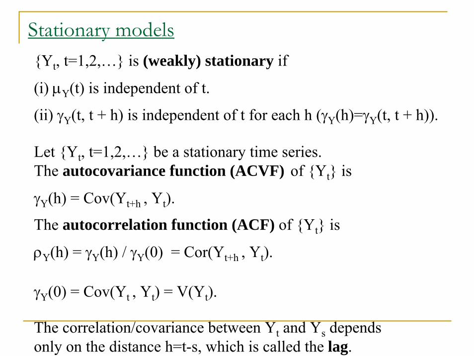
Stationary models{Yt, t=1,2,…} is (weakly) stationary if

(i) μY(t) is independent of t.

(ii) γY(t, t + h) is independent of t for each h (γY(h)=γY(t, t + h)).

Let {Yt, t=1,2,…} be a stationary time series. The autocovariance function (ACVF) of {Yt} is

γY(h) = Cov(Yt+h , Yt).

The autocorrelation function (ACF) of {Yt} is

ρY(h) = γY(h) / γY(0) = Cor(Yt+h , Yt).

γY(0) = Cov(Yt , Yt) = V(Yt).

The correlation/covariance between Yt and Ys depends only on the distance h=t-s, which is called the lag.

Stationary modelsEstimation of the ACF from an observed data {y1, y2, …, yn}.

We assume that data comes from a stationary time series.

The sample mean:

The sample autocovariance function:

The sample autocorrelation function:

∑===

n

i iY yn

yt1

1)(μ̂

( )( ) nhnyyyyn

h thn

t htY <<−−−= ∑ −

= +||

1 ||1)(γ̂

nhnhhY

YY <<−=

)0(ˆ)(ˆ)(ˆ

γγρ

Examples of models“IID noise”: {Yt, t=1,2,…} is a sequence of independent r.v’sthat are identically distributed with mean E(Yt) = 0 and variance V(Yt) = σ2 < ∞.

“White noise”: {Yt, t=1,2,…} is a sequence of uncorrelated r.v’swith mean E(Yt) = 0 and variance V(Yt) = σ2 < ∞.

IID noise ⇒ White noise

IID noise ⇔ White noise + normal distribution

μY(t) = E(Yt) = 0

γY(0) = Cov(Yt , Yt) = σ2 .

γY(h) = Cov(Yt+h , Yt) = 0 , h > 0.

Hence, stationary!

Examples of models“Random walk”: Yt = X1 + X2 + … + Xt =

= Yt-1 + Xt, t=1, 2, …,

where {Xt, t=1,2,…} is IID noise.

μY(t) = E(Yt) = 0

V(Yt) = Cov(Yt, Yt) = t σ2.

Cov(Yt+h , Yt) = t σ2.

Corr(Yt+h , Yt) = √t /√(t+h).

Depend on t, not stationary!

Examples of models

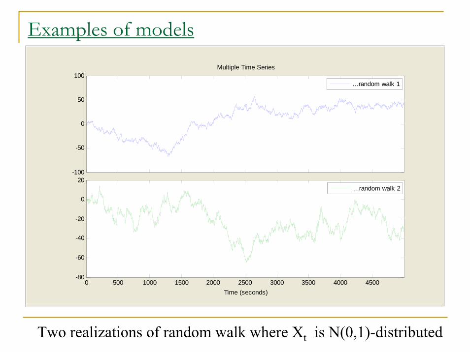
Two realizations of random walk where Xt is N(0,1)-distributed

-100

-50

0

50

100

Multiple Time Series

Time (seconds)0 500 1000 1500 2000 2500 3000 3500 4000 4500

-80

-60

-40

-20

0

20

...random walk 1

...random walk 2

Examples of modelsMA(1) (first-order moving average) process:

Yt = Xt + θ Xt-1, t = 0, ±1, ±2, …, where {Xt, t=1,2,…} is white noise and θ is a real-valued constant.

μY(t) = E(Yt) = 0

γY(0) = Cov(Yt, Yt) = (1 + θ2)σ2.

If h = ± 1 then

γY(h) = Cov(θ Xt-1, Xt) = θσ2 (otherwise 0),

Hence, stationary!

ρY(h) = γY(h) / γY(0) = θ/(1 + θ2) (otherwise 0).

Examples of models

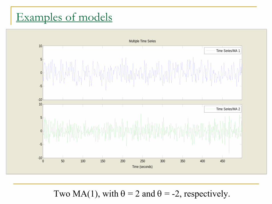
Two MA(1), with θ = 2 and θ = -2, respectively.

-10

-5

0

5

10


Time (seconds)0 50 100 150 200 250 300 350 400 450

-10

-5

0

5

10

Time Series/MA 1

Time Series/MA 2

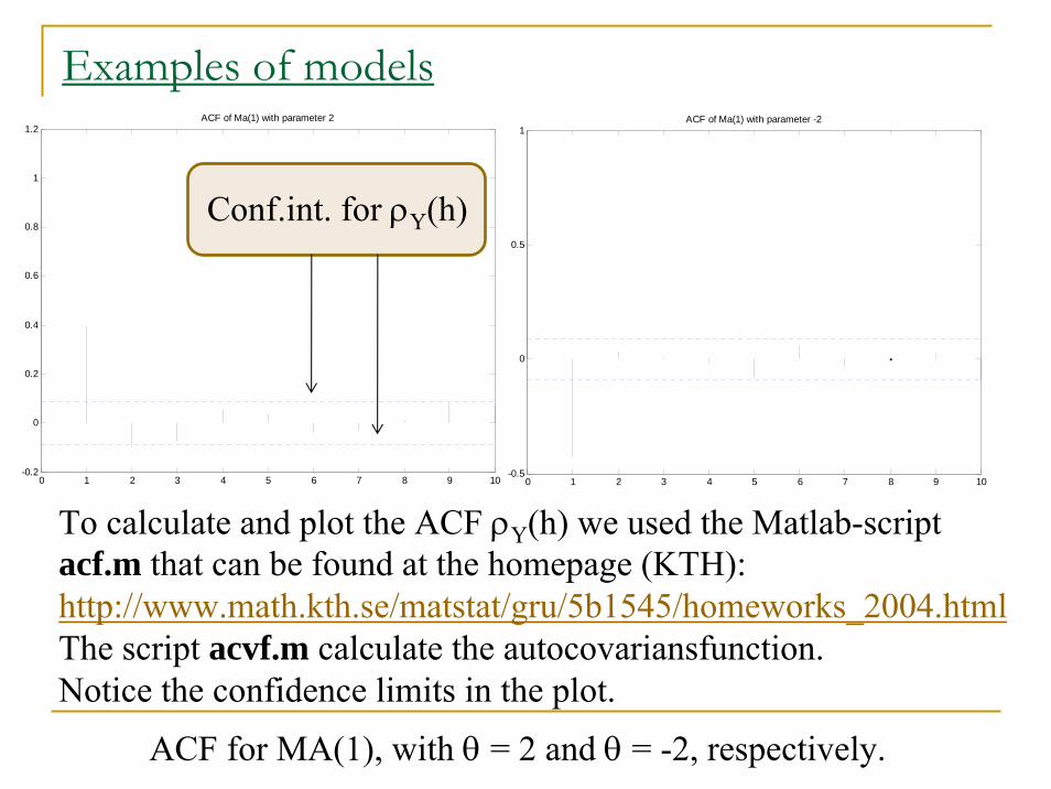
Examples of models

ACF for MA(1), with θ = 2 and θ = -2, respectively.

0 1 2 3 4 5 6 7 8 9 10-0.2

0

0.2

0.4

0.6

0.8

1

1.2ACF of Ma(1) with parameter 2

0 1 2 3 4 5 6 7 8 9 10-0.5

0

0.5

1ACF of Ma(1) with parameter -2

To calculate and plot the ACF ρY(h) we used the Matlab-script acf.m that can be found at the homepage (KTH): http://www.math.kth.se/matstat/gru/5b1545/homeworks_2004.htmlThe script acvf.m calculate the autocovariansfunction.Notice the confidence limits in the plot.

Conf.int. for ρY(h)

http://www.math.kth.se/matstat/gru/5b1545/homeworks_2004.html

Examples of models

Regression: yn = -0.042 + 0.397*yn-1

-8 -6 -4 -2 0 2 4 6-8

-6

-4

-2

0

2

4

6Regression Ma 1: Yn = -0.042 + 0.397*Yn-1

Examples of models

Regression: yn = -0.0817 - 0.0993*yn-2

-8 -6 -4 -2 0 2 4 6-8

-6

-4

-2

0

2

4

6Regression Ma 1: Yn = -0.0817 - 0.0993*Yn-2

Yn

Yn-1

Examples of modelsEstimation of MA(1): Maximum likelihood estimation is a common technique to estimate parameters, here we make it intuitively.

By using that ρY(1) = θ/(1 + θ2) and that

we can find estimates of θ for the two series.

We find the estimates 2.04 and -1.8 respectively, which is quite close to the true values 2 and -2.

Furthermore, γY(0) = (1 + θ2)σ2 and

give estimates of the variance, 1.11 and 1.15.

Close to the true variance 1.

0.3954 (1)ρ̂Y = 0.4246- (1)ρ̂Y =

5.7470 (0)γ̂Y = 4.9015 (0)γ̂Y =

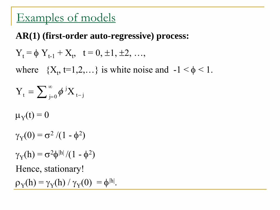
Examples of modelsAR(1) (first-order auto-regressive) process:

Yt = φ Yt-1 + Xt, t = 0, ±1, ±2, …,

where {Xt, t=1,2,…} is white noise and -1 < φ < 1.

μY(t) = 0

γY(0) = σ2 /(1 - φ2)

γY(h) = σ2φ|h| /(1 - φ2)Hence, stationary!ρY(h) = γY(h) / γY(0) = φ|h|.

∑∞

= −=0j jt

jt XY φ

Examples of models

-10

-5

0

5

10


Time (seconds)0 50 100 150 200 250 300 350 400 450

-10

-5

0

5

10

Time Series/AR 1

Time Series/AR 2

Two AR(1), with φ = 0.9 and φ = -0.9, respectively.

Examples of models

ACF for AR(1), with φ = 0.9 and φ = -0.9, respectively.

0 5 10 15 20 25 30 35 40 45 50-0.2

0

0.2

0.4

0.6

0.8

1

1.2ACF of AR(1) with parameter 0.9

0 5 10 15 20 25 30 35 40 45 50-1

-0.8

-0.6

-0.4

-0.2

0

0.2

0.4

0.6

0.8

1ACF of AR(1) with parameter -0.9

Result from the Matlab-script acf:1.0000 0.9125 0.8311 0.7561 0.6884 0.6312 0.57161.0000 -0.8986 0.8175 -0.7437 0.6805 -0.6163 0.5444

Examples of modelsEstimation of AR(1):

Here we can use that ρY(h) = φ|h| for different h. If we choose h=1

we have two estimates of φ (one for each time series).

The true ones: 0.9 and -0.9.

Furthermore, γY(h) = σ2φ|h| /(1 - φ2)

give estimates of the variance: 0.93 and 1.06.

Close to the true variance 1.

0.9125 (1)ρ̂Y = 0.8986- (1)ρ̂Y =

5.5540 (0)γ̂Y = 5.4844 (0)γ̂Y =

Examples of modelsARMA(1,1):

A combination af a AR(1) and a MA(1).

Yt = φ Yt-1 + Xt + θXt-1, t = 0, ±1, ±2, …,

where {Xt, t=1,2,…} is white noise φ + θ ≠0.

These examples of models can be extended to “higher dimensions”: AR(p), MA(q) and ARMA(p,q).

Models with trendAssume that we also have a trend in the time series:

Xt = Tt + Yt, t = 1,2,…,n

where {Yt, t=1,2,…,n} is a stationary time series.

We need to estimate and eliminate the trend.

1.Finite moving average filer:

2.Polynomial fitting (Linear regression):

qntq,X12q

1T̂ q

-qj jtt −<<+

= ∑ = +

kk10t tβ̂tβ̂β̂T̂ +++=

Models with trendLinear trend: 1+0.1*t, stationary error: AR(1) with φ = 0.9.n=100; mu=0; stdev=1;for i = 1:2*n; Y(i+1)= 0.9*Y(i) + normrnd(mu,stdev,1); end;for i = 1:n; X(i)= 1+0.1*i+Y(n+i); end;

0 10 20 30 40 50 60 70 80 90 100-2

0

2

4

6

8

10

12

14

t

X

Time series with trend, Solid line = True trend

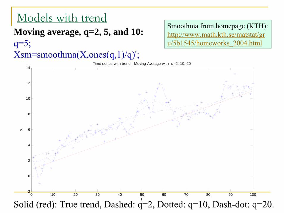
Models with trendMoving average, q=2, 5, and 10:q=5;Xsm=smoothma(X,ones(q,1)/q)';

Solid (red): True trend, Dashed: q=2, Dotted: q=10, Dash-dot: q=20.

Smoothma from homepage (KTH): http://www.math.kth.se/matstat/gru/5b1545/homeworks_2004.html

0 10 20 30 40 50 60 70 80 90 100-2

0

2

4

6

8

10

12

14

t

X

Time series with trend, Moving Average with q=2, 10, 20



Models with trendMoving average, q=2, 5, and 10:

Trend elimination:Ysm =X - Xsm; AC=acf(Ysm); AC([1:5])

ACF from the ‘trend eliminated’ series: ans = 1.0000 -0.5513 0.0866 -0.0643 -0.0253 (q=2)ans = 1.0000 0.5563 0.2690 0.0272 -0.0883 (q=10)ans = 1.0000 0.7292 0.5481 0.3847 0.2838 (q=20)

ACF from the ‘true’ AR(1)-series:ans = 1.0000 0.8177 0.6600 0.4950 0.3776

True = 1.0000 0.9 0.81 0.729 0.6561

Models with trend

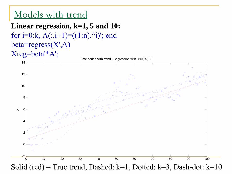
Solid (red) = True trend, Dashed: k=1, Dotted: k=3, Dash-dot: k=10

Linear regression, k=1, 5 and 10:for i=0:k, A(:,i+1)=((1:n).^i)'; endbeta=regress(X',A)Xreg=beta'*A';

0 10 20 30 40 50 60 70 80 90 100-2

0

2

4

6

8

10

12

14

t

X

Time series with trend, Regression with k=1, 5, 10

Models with trendLinear regression, k=1, 5 and 10 :

Trend elimination:Yreg =X - Xreg; AC=acf(Yreg); AC([1:5])

ACF from the ‘trend eliminated’ series: ans = 1.0000 0.7686 0.6097 0.4679 0.3820 (k=1)ans = 1.0000 0.6623 0.4377 0.2616 0.1837 (k=5)ans = 1.0000 0.8226 0.7068 0.6016 0.5348 (k=10)


True = 1.0000 0.9 0.81 0.729 0.6561

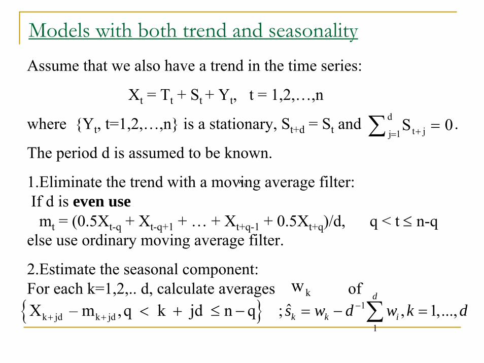
Models with both trend and seasonalityAssume that we also have a trend in the time series:

Xt = Tt + St + Yt, t = 1,2,…,n

where {Yt, t=1,2,…,n} is a stationary, St+d = St and .

The period d is assumed to be known.

1.Eliminate the trend with a moving average filter: If d is even usemt = (0.5Xt-q + Xt-q+1 + … + Xt+q-1 + 0.5Xt+q)/d, q < t ≤ n-q

else use ordinary moving average filter.

2.Estimate the seasonal component:For each k=1,2,.. d, calculate averages of

0Sd

1j jt =∑ = +

kw

kw{ }k jd k jdX – m ,q k jd n q+ + < + ≤ − 1

1

ˆ; , 1,...,d

k k is w d w k d−= − =∑

Models with both trend and seasonalityLet us add seasonality to our previous time series.

S=repmat([-5,5,2,0,-2],1,20);

Here is d=5.

0 10 20 30 40 50 60 70 80 90 100-6

-4

-2

0

2

4

6

t

S

Model for Season

Models with both trend and seasonalityThe resulting time series.

Hard to see the seasonality!

0 10 20 30 40 50 60 70 80 90 100-10

-5

0

5

10

15

20

t

X

Time series with trend and season

Models with both trend and seasonalityThe resulting time series.

Now it is easier to see the seasonality!

0 10 20 30 40 50 60 70 80 90 100-10

-5

0

5

10

15

20

t

X

Time series with trend and season

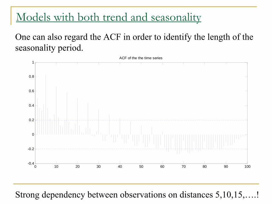
Models with both trend and seasonalityOne can also regard the ACF in order to identify the length of the seasonality period.

Strong dependency between observations on distances 5,10,15,….!

0 10 20 30 40 50 60 70 80 90 100-0.4

-0.2

0

0.2

0.4

0.6

0.8

1ACF of the the time series

Models with both trend and seasonality1. The estimation of the trend with moving average (q=5).

m=smoothma(X,ones(q)/q)';

0 10 20 30 40 50 60 70 80 90 100-4

-2

0

2

4

6

8

10

12

t

m

The m-estimate of the Trend

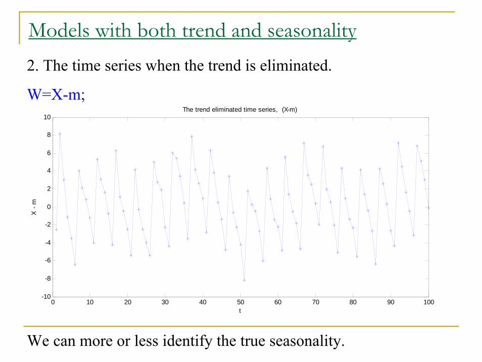
Models with both trend and seasonality2. The time series when the trend is eliminated.

W=X-m;

We can more or less identify the true seasonality.

0 10 20 30 40 50 60 70 80 90 100-10

-8

-6

-4

-2

0

2

4

6

8

10

t

X -

m

The trend eliminated time series, (X-m)

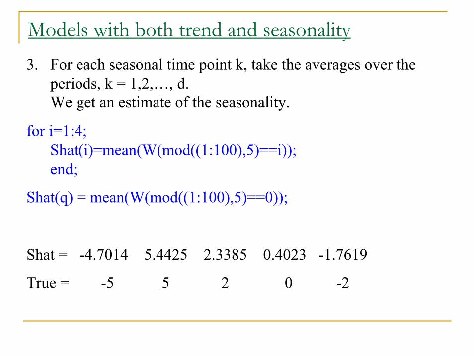
Models with both trend and seasonality3. For each seasonal time point k, take the averages over the

periods, k = 1,2,…, d.We get an estimate of the seasonality.

for i=1:4; Shat(i)=mean(W(mod((1:100),5)==i));end;

Shat(q) = mean(W(mod((1:100),5)==0));

Shat = -4.7014 5.4425 2.3385 0.4023 -1.7619

True = -5 5 2 0 -2

Models with both trend and seasonality4. Withdraw the seasonality from the original time series X (with

trend).

0 10 20 30 40 50 60 70 80 90 100-4

-2

0

2

4

6

8

10

12

14

t

X -

S

The season eliminated time series

Models with both trend and seasonality5. It remain to eliminate the trend.

This could be done e.g. with moving average or regression.If we use moving average with q= 5

0 10 20 30 40 50 60 70 80 90 100-4

-2

0

2

4

6

8

10

12

14

t

XT

Season eliminated Time series, Moving Average with q=5

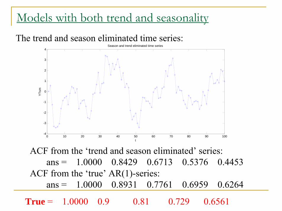
Models with both trend and seasonalityThe trend and season eliminated time series:

ACF from the ‘trend and season eliminated’ series: ans = 1.0000 0.8429 0.6713 0.5376 0.4453


True = 1.0000 0.9 0.81 0.729 0.6561

0 10 20 30 40 50 60 70 80 90 100-4

-3

-2

-1

0

1

2

3

4

t

YTs

m

Season and trend eliminated time series

Bootstrap for time series

IntroductionThe observations are time dependent:we cannot resample from the empirical distribution function Fn(or resampling with replacement) which does not reflect the timedependency.

Two main approaches:

-Using a parametric model for resampling

-Using blocks of the data to simulate the time series.

– Typeset by FoilTEX – 1

Model based resampling

We use standard time series models(ARMA)for defining the datagenerating process.

- Let {Xt} be a second order stationary time series, with zero meanand autocovariance function γk: for all t, k we have

E(Xt) = 0;Cov(Xt, Xt+k) = γk.

- The autocorrelation function is ρk = γk/γ0 for all k = 0, 1, 2, ....

- Some basic models


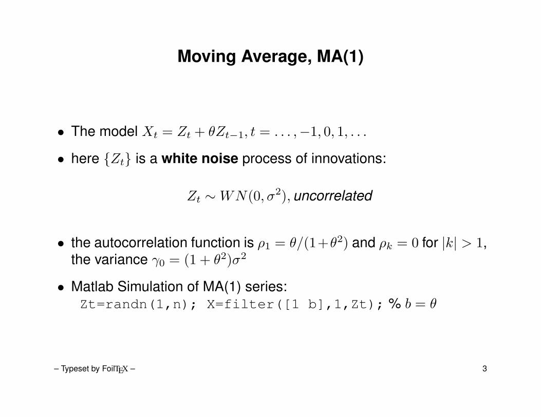
Moving Average, MA(1)

• The model Xt = Zt + θZt−1, t = . . . ,−1, 0, 1, . . .

• here {Zt} is a white noise process of innovations:

Zt ∼WN(0, σ2),uncorrelated

• the autocorrelation function is ρ1 = θ/(1+θ2) and ρk = 0 for |k| > 1,the variance γ0 = (1 + θ2)σ2

• Matlab Simulation of MA(1) series:Zt=randn(1,n); X=filter([1 b],1,Zt); % b = θ


AutoRegressive, AR(1)

• The model Xt = φXt−1 + Zt, t = . . . ,−1, 0, 1, . . .

• here |φ| < 1, and {Zt} is a white noise WN(0, σ2), Xt =∑∞0 φkZt−k

• the variance, Cov(Xt−k, Zt) = 0, k ≥ 1, γ0 = V ar(Xt) =V ar(φXt−1 + Zt) = φ2γ0 + σ2;and γ0 = σ2/(1− φ2).

• the autocorrelation function is ρk = φ|k| and for k = 1,

φ = ρ1 = γ1/γ0

• Matlab Simulation AR(1) series:Zt=randn(1,n); X=filter(1,[1 a],Zt); % a = −φ


AutoRegressive Moving Average, ARMA(p,q)

• The model

Xt =p∑k=1

φkXt−k + Zt +q∑

k=1

θkZt−k,

{Zt} is a white noise WN(0, σ2).

• Conditions on the coefficients to obtain a stationary process.

• Matlab Simulation of ARMA(1,1) series:Zt=randn(1,n); X=filter([1 b],[1,a],Zt); % b =θ, a = −φ


The bootstrap

• Fit the model to the data

• Constructed the residuals from the fitted model

• Re-center the residuals(mean zero as Zt)

• Generate new series by incorporating random samples from thefitted residuals in the fitted model


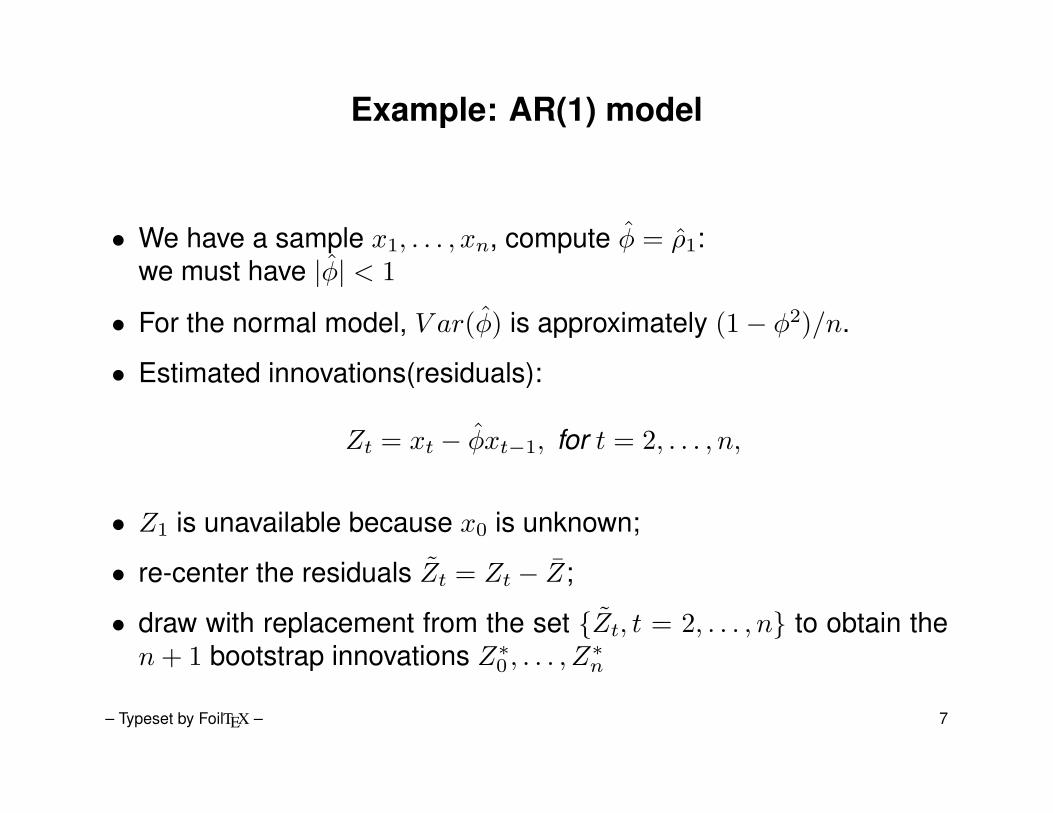
Example: AR(1) model

• We have a sample x1, . . . , xn, compute φ̂ = ρ̂1:we must have |φ̂| < 1

• For the normal model, V ar(φ̂) is approximately (1− φ2)/n.

• Estimated innovations(residuals):

Zt = xt − φ̂xt−1, for t = 2, . . . , n,

• Z1 is unavailable because x0 is unknown;

• re-center the residuals Z̃t = Zt − Z̄;

• draw with replacement from the set {Z̃t, t = 2, . . . , n} to obtain then+ 1 bootstrap innovations Z∗0 , . . . , Z∗n


• Then we define the bootstrap sample X∗0 , . . . , X∗n:

X∗0 = Z∗0

X∗t = φ̂X∗t−1 + Z∗t , t = 1, ..., n

• Then compute φ̂∗ from the observation X∗1 , ..., X∗n, and proceed asusual.

• In fact, the series {X∗t } is not stationary. For improving this:

– Start the series of X∗t at t = −k (in place of t = 0) and thendiscard the observations X∗−k, ..., X

∗0 .

– If k is large enough, the resulting bootstrap sample will beapproximatively stationary.

Can be used for testing hypothesis,confidence intervals(bootstrap t-percentile,. . .), prediction,. . .


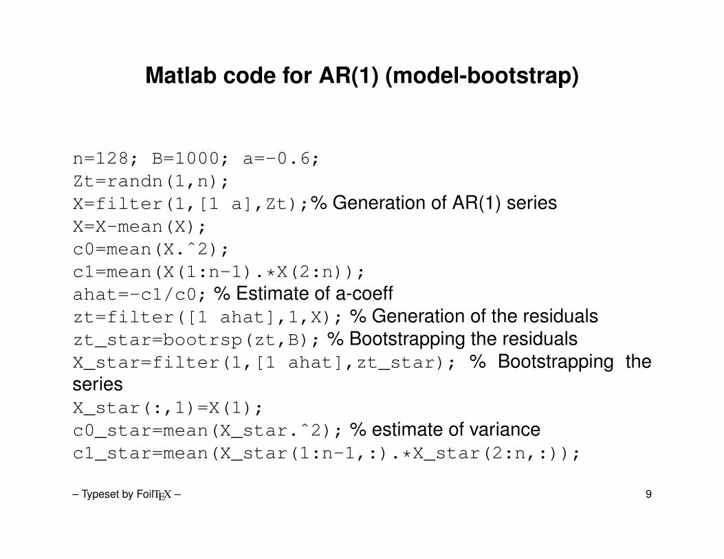
Matlab code for AR(1) (model-bootstrap)

n=128; B=1000; a=-0.6;Zt=randn(1,n);X=filter(1,[1 a],Zt);% Generation of AR(1) seriesX=X-mean(X);c0=mean(X.ˆ2);c1=mean(X(1:n-1).*X(2:n));ahat=-c1/c0; % Estimate of a-coeffzt=filter([1 ahat],1,X); % Generation of the residualszt_star=bootrsp(zt,B); % Bootstrapping the residualsX_star=filter(1,[1 ahat],zt_star); % Bootstrapping theseriesX_star(:,1)=X(1);c0_star=mean(X_star.ˆ2); % estimate of variancec1_star=mean(X_star(1:n-1,:).*X_star(2:n,:));


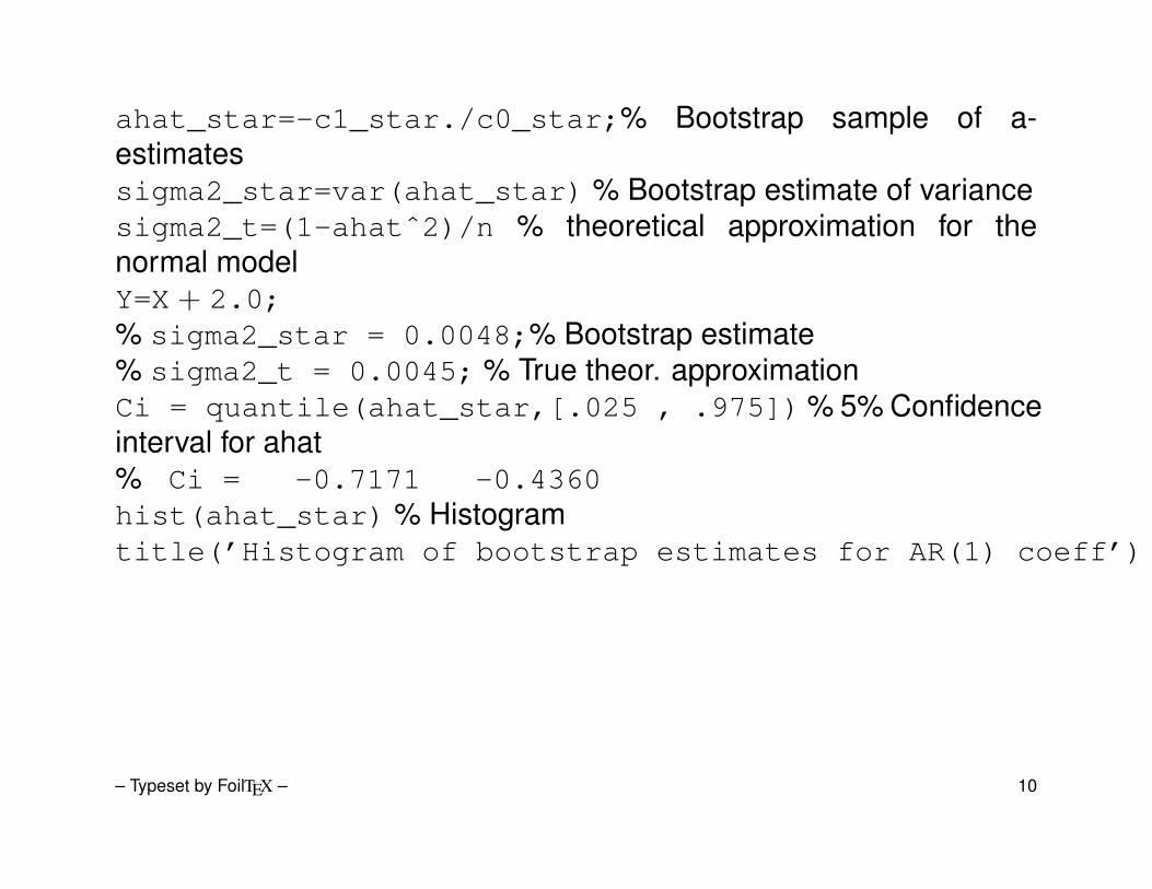
ahat_star=-c1_star./c0_star;% Bootstrap sample of a-estimatessigma2_star=var(ahat_star) % Bootstrap estimate of variancesigma2_t=(1-ahatˆ2)/n % theoretical approximation for thenormal modelY=X + 2.0;% sigma2_star = 0.0048;% Bootstrap estimate% sigma2_t = 0.0045; % True theor. approximationCi = quantile(ahat_star,[.025 , .975])% 5% Confidenceinterval for ahat% Ci = -0.7171 -0.4360hist(ahat_star) % Histogramtitle(’Histogram of bootstrap estimates for AR(1) coeff’)


−1 −0.9 −0.8 −0.7 −0.6 −0.5 −0.4 −0.30

50

100

150

200

250

300

350

400Histogram of bootstrap estimates for AR(1) coeff

Histogram of bootstrap estimates for AR(1) coefficient, a = −φ = −0.6


Block resampling

The idea here is not to draw from innovations defined with respectto a particular model but on blocks of consecutive observations. Wedon’t need a model here...The algorithm is as follows:

• Divide the data into b non-overlapping blocks of length l. So wesuppose n = lb.


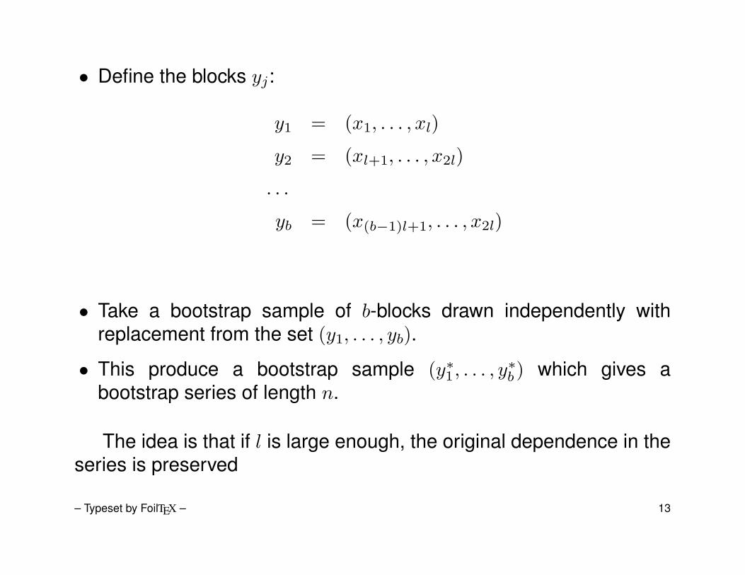
• Define the blocks yj:

y1 = (x1, . . . , xl)

y2 = (xl+1, . . . , x2l)

. . .

yb = (x(b−1)l+1, . . . , x2l)

• Take a bootstrap sample of b-blocks drawn independently withreplacement from the set (y1, . . . , yb).

• This produce a bootstrap sample (y∗1, . . . , y∗b ) which gives a

bootstrap series of length n.

The idea is that if l is large enough, the original dependence in theseries is preserved


• So we hope that the bootstrap statistics T (X∗) will haveapproximatively the same distribution as the statistics T (X) in thereal world, with the real series...

• On the other hand we must have enough blocks b to estimate withaccuracy the bootstrap distribution of T (X∗)

- A good balance: should be of the order O(nγ) where γ ∈ (0, 1),so b = n/l→∞ as n→∞.

- There are several variants of the method (overlapping blocks,blocks of blocks, blocks of random length, pre-whitening,...).

- Theoretical works are still in progress(optimal choice of l, etc.)


Matlab code for AR(1)(block-bootstrap)

Function bpestcir from Bootstrap Matlab Toolbox

% [est,estvar]=bpestcir(X,estfun,L1,M1,Q1,L2,M2,Q2,B,PAR1,...) %% The program calculates the estimate and the variance% of an estimator of a parameter from the input vector X.% The algorithm is based on a circular block bootstrap% and is suitable when the data is weakly correlated.%% Inputs:% x - input vector data% estfun - the estimator of the parameter given as a Matlab function% L1 - number of elements in the first block (see ”segmcirc.m”)% M1 - shift size in the first block


% Q1 - number of segments in the first block% L2 - number of elements in the second block (see ”segmcirc.m”)% M2 - shift size in the second block% Q2 - number of segments in the second block% B - number of bootstrap resamplings (default B=99)% PAR1,... - other parameters than x to be passed to estfun%% Outputs:% est - estimate of the parameter% estvar - variance of the estimator%% Example:% [est,estvar]=bpestcir(randn(1000,1),’mean’,50,50,50,10,10,10);

[est,estvar]=bpestcir(Y,’mean’,20,20,20,10,10,10)% est = 1.9633; estvar = 0.0212;% est_tr=2.0 mean[est,estvar]=bpestcir(Y,’var’,20,20,20,10,10,10)


% Variance estimation c0% est = 1.7843; estvar = 0.0250 ;% est_tr=1.5625 variance

% Compare with the white noise% sigma_iid=var_mhat_iid=c0/n= 0.0109% Theor. estimate for the variance of mean for the white noise% Var(mhat)=estvar=0.0212

References

Simar, L. (2008) An Invitation to the Bootstrap: Panacea for Statistical Inference?Handouts. Dept. Stat., Louvain University.

A. M. Zoubir, D. R. Iskander, Bootstrap techniques for signal processing.Cambridge Un Press, 2004

A. M. Zoubir, D. R. Iskander, Bootstrap Matlab Toolboxhttp://www.csp.curtin.edu.au/downloads/bootstrap_toolbox.html


stat modeling and time series

Documents