Stata Review: Part II

Biost/Epi 536 Discussion SectionOctober 13, 2009

Indicator (Dummy) Variables• Created from an existing categorical variable (e.g., bmicat)• Assigned value of 0 or 1

• 1, if the condition is true• 0, if the condition is false

-------------------------------------------------------------------bmicat BMI (categorical)------------------------------------------------------------------- type: numeric (float) label: bmicat_label range: [0,3] units: 1 unique values: 4 missing .: 5/60

tabulation: Freq. Numeric Label 10 0 Underweight 17 1 Normal 17 2 Overweight 11 3 Obese 5 .

Indicator (Dummy) VariablesExample: bmicat

Xb0 =

1 underweight

0 otherwise

Xb1 =

1 normal

0 otherwise

Xb2 =

1 overweight

0 otherwise

Xb3 =

1 obese

0 otherwise

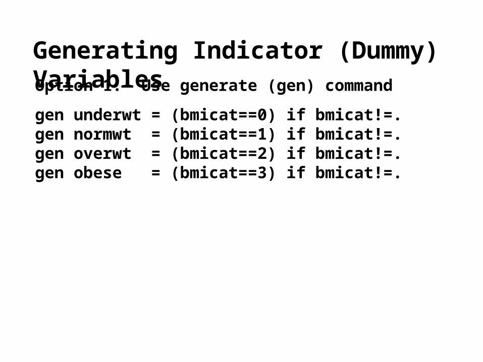
Generating Indicator (Dummy) VariablesOption 1: Use generate (gen) command

gen underwt = (bmicat==0) if bmicat!=.gen normwt = (bmicat==1) if bmicat!=.gen overwt = (bmicat==2) if bmicat!=.gen obese = (bmicat==3) if bmicat!=.

Generating Indicator (Dummy) VariablesOption 1: Use generate (gen) command

. list bmicat underwt normwt overwt obese in 31/40 +-------------------------------------------------+ | bmicat underwt normwt overwt obese | |-------------------------------------------------| 31. | Normal 0 1 0 0 | 32. | Overweight 0 0 1 0 | 33. | . . . . . | 34. | Overweight 0 0 1 0 | 35. | Underweight 1 0 0 0 | |-------------------------------------------------| 36. | Normal 0 1 0 0 | 37. | Overweight 0 0 1 0 | 38. | Obese 0 0 0 1 | 39. | Overweight 0 0 1 0 | 40. | Underweight 1 0 0 0 | +-------------------------------------------------+

Generating Indicator (Dummy) VariablesOption 2: Use tabulate command with generate option

tabulate bmicat, generate(bmigrp)

. tabulate bmicat, generate(bmigrp)

BMI |(categorica | l) | Freq. Percent Cum.------------+-----------------------------------Underweight | 10 18.18 18.18 Normal | 17 30.91 49.09 Overweight | 17 30.91 80.00 Obese | 11 20.00 100.00------------+----------------------------------- Total | 55 100.00

Generating Indicator (Dummy) VariablesOption 2: Use tabulate command with generate option

. list bmicat bmigrp1-bmigrp4 in 31/40 +-----------------------------------------------------+ | bmicat bmigrp1 bmigrp2 bmigrp3 bmigrp4 | |-----------------------------------------------------| 31. | Normal 0 1 0 0 | 32. | Overweight 0 0 1 0 | 33. | . . . . . | 34. | Overweight 0 0 1 0 | 35. | Underweight 1 0 0 0 | |-----------------------------------------------------| 36. | Normal 0 1 0 0 | 37. | Overweight 0 0 1 0 | 38. | Obese 0 0 0 1 | 39. | Overweight 0 0 1 0 | 40. | Underweight 1 0 0 0 | +-----------------------------------------------------+

Graphing in Stata 10

Creating HistogramsStata command: hist

Example: Histogram of height, by sex

hist height, by(sex)

0.0

2.0

4.0

6

50 60 70 80 50 60 70 80

0 1D

ensi

ty

heightGraphs by sex

Creating HistogramsStata command: histAttach value labels to variable(s) of interestUse formatting options

Example revisited: Histogram of height, by sex

hist height, by(sex, title(“Distribution of

height by sex”) note(“”)) xtitle(“height(in)”)

scheme(s1mono)

0.0

2.0

4.0

6

50 60 70 80 50 60 70 80

female male

Den

sity

height(in)

Distributions of height by sex

Creating Box PlotsStata command: graph box

Example: Box plot of height, by sex

graph box height, by(sex, title(Boxplots of

height by sex) note(“”)) ytitle(height(in))

scheme(s1mono)

50

60

70

80

female male

hei

ght(

in)

Boxplots of height by sex

Creating Box PlotsStata command: graph boxNow using over option

Example: Box plot of height, by sex

graph box height, over(sex) title(“Boxplots

of height by sex”) ytitle(“height(in)”)

scheme(s1mono)

5060

7080

heig

ht(in

)

female male

Boxplots of height by sex

Creating Scatter PlotsStata command: scatter

Example: Scatter plot of height and weight

scatter height weight

50

60

70

80

hei

ght

100 150 200weight

Creating Scatter PlotsStata command: scatter

Example:

Scatter plot of height and weight by sex, with lowess smoothing

twoway (scatter height weight if sex==0) ///

(scatter height weight if sex==1) ///

(lowess height weight if sex==0) ///

(lowess height weight if sex==1)

50

60

70

80

100 150 200weight

height heightlowess height weight lowess height weight

Creating Scatter PlotsStata command: scatterUse formatting options

Example revisited: Scatter plot of height and weight by sex, with lowess smoothing

twoway(scatter height weight if sex==0,ms(D))(scatter height weight if sex==1, ms(Oh))(lowess height weight if sex==0)(lowess height weight if sex==1),scheme(s2mono)legend(col(2)order(1 “females” 2 “males” 3 “lowessfemales” 4 “lowess males”))xtitle(weight(lbs)) ytitle(height(in))title(Height vs. weight by sex)xlab(100(25)200) ylab(50(5)80)

50

55

60

65

70

75

80

hei

ght (

in)

100 125 150 175 200weight (lbs)

females maleslowess females lowess males

Height vs. weight by sex

Combining GraphsStata command: graph combine

Example: Histogram and box plot of height

hist height, scheme(s1mono) name(hist)

graph box height, scheme(s1mono) name(box)

graph combine hist box, scheme(s1mono) title(distribution of height)

0.0

2.0

4.0

6D

ensi

ty

50 55 60 65 70 75height 5060

7080

heig

ht

distribution of height