Federal Reserve Bank of Dallas Globalization and Monetary Policy Institute

Working Paper No. 39 http://www.dallasfed.org/assets/documents/institute/wpapers/2009/0039.pdf

State-Dependent Pricing, Local-Currency

Pricing, and Exchange Rate Pass-Through*

Anthony Landry Federal Reserve Bank of Dallas

September 2009

Abstract This paper presents a two-country DSGE model with state-dependent pricing as in Dotsey, King, and Wolman (1999) in which firms price-discriminate across countries by setting prices in local currency. In this model, a domestic monetary expansion has greater spillover effects to foreign prices and foreign economic activity than an otherwise identical model with time-dependent pricing. In addition, the predictions of the state-dependent pricing model match the business-cycle moments better than the predictions of the time-dependent pricing model when driven by monetary policy shocks. JEL codes: F41, F42

* Anthony Landry, Research Department, Federal Reserve Bank of Dallas, Research Department, 2200 N. Pearl Street, Dallas, TX, 75201. 214-922-5831. Anthony.Landry@dal.frb.org. This paper is a revised and rewritten version of Research Department Working Paper 0706. I would like to thank Marianne Baxter, Russell Cooper, Michael Devereux, Simon Gilchrist, Michel Juillard, Robert G. King, Sylvain Leduc, two anonymous referees, and seminar participants at Boston University, the Federal Reserve Bank of Dallas, and the 47th Annual Meeting of the Société Canadienne de Science Économique for helpful comments and suggestions. The views in this paper are those of the author and do not necessarily reflect the views of the Federal Reserve Bank of Dallas or the Federal Reserve System.

1 Introduction

What are the implications of monetary policy shocks when exchange rate pass-

through to prices is sluggish and incomplete? To answer this question, the open-

economy macroeconomic literature has focused on dynamic general equilibrium mod-

els with nominal rigidities in which monopolistic �rms price-discriminate across

countries by setting prices in local currency. This mechanism acts to limit the pass-

through from exchange rate changes to foreign prices and largely insulates foreign

economies from domestic monetary policy shocks. Good examples of these mod-

els include Betts and Devereux (2000), Chari et al. (2002), and Kollmann (2001).

However, a much criticized but standard element of this literature is the exogenously

imposed timing of the opportunity �rms have for nominal price adjustments.

I address this critique by developing a two-country version of the dynamic gen-

eral equilibrium model with state-dependent pricing (SDP) from Dotsey, King, and

Wolman (1999) in which �rms price-discriminate across markets by setting price in

local currency.1 In the model, �rms pay a single menu cost to have the opportunity

to change their domestic and export prices. The SDP pricing structure implies that

the degree of price rigidity depends on the state of the economy: Over the business

cycle, this pricing structure generates discrete and occasional price adjustments by

�rms in light of variations in demand and cost conditions. Those changes in eco-

nomic environment a¤ect not only the intensive margin�the level of price adjustment

undertaken by price-adjusting �rms�but also the extensive margin�the fraction of

�rms actively engaged in price adjustment. I �nd that a domestic monetary expan-

sion generates larger spillover e¤ects to foreign prices and foreign economic activity

under the SDP model, than a similar model with time-dependent pricing (TDP)

because of the interplay between the intensive and extensive margins.

In local-currency pricing models, a domestic monetary expansion a¤ects �rms�

pro�ts on exported goods via two channels: a depreciation of the dollar, and an

increase in marginal cost generated by higher domestic demand. On one hand, the

dollar depreciation increases pro�ts as �rms get more dollar for every unit sold in

the foreign market. On the other, the increase in marginal cost shrinks pro�ts. In

the TDP model, these two e¤ects roughly balance out over the expected horizon of

price rigidities. Therefore, �rms barely adjust export prices following a domestic

1 In my previous work (Landry 2009), I look at the implications of monetary policy shocks in a

two-country model with state-dependent pricing in which the law-of-one price holds.

1

monetary expansion. In the SDP model, �rms have the ability to change their prices

in light of demand and cost conditions. On impact, the �rst e¤ect dominates and

�rms decide to lower their export prices to attract foreign demand. However,

the second e¤ect takes over after a few quarters and �rms start raising export

prices. Over the business cycle, these export price movements generate �uctuations

in foreign expenditure without any actions in foreign monetary policy. This result

contradicts the current wisdom and has important implications for the design of

international monetary policy in a local-currency pricing environment.

I take the model to the data by choosing parameter values to replicate the trade

relationship between the U.S. and Canada. I introduce two features to the model to

better capture the business-cycle moments observed in the data. First, I add vari-

able demand elasticity, following the work of Kimball (1995), to generate inertia in

prices and adjustment fractions. Second, I introduce investment with variable cap-

ital utilization, following the work of Baxter and Farr (2005). Investment is needed

to generate the relative volatility of consumption to output, while variable capital

accumulation is needed to smooth investment demand and trade �ows. Overall,

the SDP model�s predictions match the business-cycle moments better than the

predictions of the TDP model when driven by monetary policy shocks.

This paper is related to the development of other local-currency pricing SDP

models. For example, Gopinath et al. (2009) study the endogenous currency choice

�rms face when setting prices, while Gopinath and Itskhoki (2009) study the rela-

tion between the frequency of price adjustment and the level of exchange rate pass-

through. Floden and Wilander (2006) focus on exchange rate pass-through and the

volatility of import prices. These three studies use a partial equilibrium approach

where �rms�decisions are driven by productivity or exchange rate shocks. In con-

trast, I use a general equilibrium approach to study the international business-cycle

transmission of monetary shocks. The nature of the dynamic general equilibrium

approach implies �uctuations in prices and exchange rate pass-through that a¤ects

foreign economic conditions.

Section 2 of this paper describes the open-economy SDP model. Section 3

presents the model�s solution and parameterization. Section 4 discusses the model�s

implications. First, I analyze the endogenous evolution of price distributions in

response to a domestic monetary expansion, describe the way these distributions

in�uence exchange rate pass-through and international economic activity, and con-

trast the implications of the SDP model with a corresponding TDP model that is

2

used as a reference case because of its popularity in the current literature. Then,

I look at the business-cycle implications of the model in which the world economy

experiences shocks to the U.S. and Canadian money stocks. I also examine the

sensitivity of my �ndings by varying assumptions about the SDP model benchmark.

Section 5 concludes.

2 The Model

The world economy consists of two countries. Each country is populated by a repre-

sentative household, a continuum of monopolistic �rms, and a monetary authority.

Households purchase goods produced in both countries for consumption and invest-

ment, and supply labor and capital on a competitive basis. Firms rent labor and

capital from the domestic market to produce goods. They can price-discriminate

across countries and set prices in local currency. The distinctive feature of the

model is that in each period, �rms can change their prices by paying a menu cost.

If a �rm decides to pay the menu cost, it has the opportunity to change its domestic

and export prices. Once prices are set, �rms must satisfy demand.

In what follows, each variable is represented by a country�i.e. i; j = 1; 2 for

Country 1 (U.S.) and Country 2 (Canada)�and time subscripts. When three sub-

scripts are present, the �rst denotes the country of production, the second denotes

the country of consumption or investment, and the third denotes time.

2.1 Households

Households are identical across countries except for the local bias introduced in

consumption and investment. They make consumption ci;t and labor supply ni;tdecisions to maximize expected lifetime utility:

Et

1Xt=0

�t�

1

1� �c1��i;t � �

1 + �n1+�i;t

�; for i = 1; 2. (1)

The momentary utility function is separable in consumption and leisure. The para-

meter � represents the discount factor, � represents the intertemporal elasticity of

substitution, and � represents the elasticity of labor supply.

The households�optimal consumption allocations are de�ned as a constant elas-

ticity of substitution (CES) composite of domestic and imported consumption, such

3

that

c1;t =

�(1� �1)

1 c

�1

1;1;t + �1

1 c �1

2;1;t

� �1

, (2)

c2;t =

�(1� �2)

1 c

�1

2;2;t + �1

2 c �1

1;2;t

� �1

.

In these equations, the parameters �i for i = 1; 2 represent the steady-state shares

of imports into consumption, and represents the elasticity of substitution between

domestic and imported goods. The goal of the household is to minimize expenditure

such that equation (2) holds. The solution to the minimization problem yields the

following optimal consumption quantities:

c1;1;t = (1� �1)�PP1;1;tPC1;t

�� c1;t, c2;1;t = �1

�PP2;1;tPC1;t

�� c1;t,

c2;2;t = (1� �2)�PP2;2;tPC2;t

�� c2;t, c1;2;t = �1

�PP1;2;tPC2;t

�� c2;t,

(3)

where PCi;t for i = 1; 2 represents the aggregate consumption prices, and PPi;j;t for

i = 1; 2 represents the aggregate producer prices.

Households also choose an optimal amount of capital through investment ii;t.

Investment decisions are made following the capital accumulation equations:

ki;t+1 = (1� � (ui;t)) ki;t + ��ii;tki;t

�ki;t for i = 1; 2, (4)

where ki;t denotes the capital stocks, � the depreciation function with �0 > 0 and

�00 < 0, ui;t the utilization rates of capital, and � the capital adjustment cost with

�0 > 0 and �00 < 0. The households�optimal investment allocations are identical to

the consumption allocations (2).

Given these optimal choices, aggregate consumption and investment prices are

a weighted sum of domestic and imported goods prices:

P c1;t = P i1;t =�(1� �1) (PP1;1;t)1� + �1

�PP2;1;t

�1� � 11�

, (5)

P c2;t = P i2;t =�(1� �2) (PP2;2;t)1� + �2

�PP1;2;t

�1� � 11�

.

The benchmark economy features complete risk pooling to isolate the role of

SDP. This implies that households can freely reallocate risk through a complete set

of state-contingent nominal bonds bi;t and corresponding stochastic discount factor

4

Dt, such that Et[Dt+1bi;t+1] =Pst+1

�(st+1jst)D(st+1jst)bi(st+1), where �(st+1jst)denotes the probability of the state of nature st+1 given st. The households also

receive capital payments Qi;t from capital services, nominal wages Wi;t from labor

services, and a series of dividend payments Zi;t from �rms. In each country, capital

services xi;t are the product of the capital stock and the utilization rate. The se-

quence of intertemporal budget constraints can be represented in terms of aggregates

as

P ci;tci;t + Pii;tii;t + Et[Dt+1bi;t+1] � bi;t +Qi;txi;t +Wi;tni;t + Zi;t for i = 1; 2. (6)

The problem for households is then to choose consumption, investment, labor,

and portfolio holdings to maximize lifetime utility (1) subject to a sequence of

intertemporal budget constraints (6) and allocation of time. The maximization

problem implies that the ratios of marginal utilities of consumption �i;t are equalized

across countries, or qt = � � �2;t=�1;t. The real exchange rate is de�ned as qt =St �

�PC2;t=P

C1;t

�, where St is the dollar price of one unit of foreign currency, and �

re�ects initial wealth di¤erences.

Finally, the level of nominal aggregate demand is governed by a cash-in-advance

constraint Mi;t = P ci;tci;t + Pii;tii;t for i = 1; 2, along with money supply rules.

2.2 Firms

A continuum of monopolistically competitive �rms is located on the unit interval

and indexed by z in each country. At any date t, a �rm is identi�ed by its current

prices and its current menu cost of price adjustment �i;t(z) 2�0; B

�. The menu cost

is denominated in labor hours and drawn from a time-invariant distribution G(�i;t)

common across all �rms in country i. Since the indices z are uncorrelated over time,

and there are no other state variables attached to individual �rms, price-adjusting

�rms in the same country �nd it optimal to charge a common price in each market.

I restrict the analysis to positive steady-state in�ation rates so that the bene�t of

price adjustment becomes in�nitely large as the number of periods for which the

price has been �xed grows. Given that the support of the distribution G(�i;t) is

�nite, there is a �nite fraction of vintages in each country Fi, a vintage being a

measure of �rms with common domestic and export prices.

5

2.2.1 Firms�demand and Aggregate Prices

I introduce variable demand elasticity following the work of Kimball (1995), as in

the open-economy model of Bouakez (2005), Gopinath et al. (2009), Gopinath and

Itskhoki (2009), Gust et al. (2006). In contrast to a Dixit-Stiglitz demand, variable

demand elasticity makes it more costly for adjusting �rms to get their prices out of

line with prices set by other �rms. However, as opposed to TDP models in which

the timing of price adjustment is �xed, SDP and variable demand elasticity increase

the interaction between �rms: Variable demand elasticity makes it desirable for

�rms to keep their prices similar, while SDP makes it feasible for them to do so.

Consider the following expenditure-minimization problem for each country:

mindi;j;t(z)

Z 1

0

Pi;j;t(z)di;j;t(z)dz subject toZ 1

0

�

�di;j;t(z)

di;j;t

�dz = 1 for i; j = 1; 2, (7)

where

�

�di;j;t(z)

di;j;t

�=

1

(1 + ') %

�(1 + ')

�di;j;t(z)

di;j;t

�� '

�%��1 +

1

(1 + ') %

�. (8)

In these equations, di;j;t represents the demand for goods produced in country

i and purchased in country j. Each �rm produces a di¤erentiated product such

that Pi;j;t(z) identi�es the price charged by an individual �rm with relative demand

di;j;t(z)=di;j;t. The demand aggregator � is such that an aggregate producer price

index PPi;j;;t holds in each market. The demand aggregator � is an increasing and

concave function re�ecting diminishing demand elasticity and is de�ned over the

parameters ' and %. The parameter ' determines the curvature of the demand

function, while % determines the elasticity of demand at average product prices. A

nice property of this speci�cation is that the Dixit-Stiglitz aggregator is a special

case represented by ' = 0.

The demand aggregator de�nes �rms�relative demand as a function of individual

and aggregate prices, and of the curvature parameters of the demand function

di;j;t (z)

di;j;t= f

Pi;j;t(z)

PPi;j;t; '; %

!for i; j = 1; 2. (9)

Finally, the aggregate producer prices follow a weighted sum of prices over indi-

vidual �rm demand ratios

PPi;j;t =

Z 1

0Pi;j;t(z)

�di;j;t(z)

di;j;t

�dz for i; j = 1; 2. (10)

6

2.2.2 Production

Supply is demand driven, and production by an individual �rm is the sum of demand

in the domestic and export markets:

yi;t(z) = yi;i;t(z) + yi;j;t(z) for i; j = 1; 2, (11)

where

yi;j;t(z) = f

Pi;j;t(z)

PPi;j;t; '; %

!� di;j;t for i; j = 1; 2. (12)

Equation (12) illustrates that production by an individual �rm depends on its

price relative to other domestic �rms (PPI) and on the market�s demand. Market

demand is determined by the sum of consumption and investment demand such that

di;j;t = ci;j;t + ii;j;t for i; j = 1; 2.

Labor used for price adjustment is denoted nai;t(z), and labor used for production

is denoted nyi;t(z). Total labor employed by a �rm is thus nai;t(z) + nyi;t(z) = ni;t(z).

Production by an individual �rm is

yi;t(z) = x1�&i;t (z) � n&i;t(z) for i; j = 1; 2. (13)

where & represents the labor share in production.

2.2.3 Pricing Policy

In both SDP and TDP frameworks, the �rms�optimal decision can be representedusing a dynamic programming approach: Given the level of demand, the currentmenu cost of price adjustment, the current real price, the prevailing real capitalservice, and the real wage, individual �rms decide whether or not to adjust theirprices with respect to a state vector st. Accordingly, each �rm z that has changedits price f periods ago has a real value function of the form

v�pCi;i;t; p

Ci;j;t�i;t(z)jst

�=

max

8><>:vi;f;t = �

�pCi;i;f;t; p

Ci;j;f;tjst

�+ �Et�i;t;t+1v

�pCi;i;f+1;t+1; p

Ci;j;f+1;t+1; �i;t+1(z)jst+1

�;

vi;0;t = maxbpCi;i;t

;bpCi;j;t

��bpCi;i;t; bpCi;j;tjst�+ �Et�i;t;t+1v

�bpCi;i;t+1; bpCi;j;t+1�i;t+1(z)jst+1�� wi;t�i;t(z)

9>=>;for i; j = 1; 2, i 6= j, (14)

with the value if the individual �rm does vi;0;t or does not vi;f;t adjust, and the opti-

mal prices chosen by adjusting �rms bpCi;i;f;t = Pi;i;f;t=PCi;t, and bpCi;j;f;t = StPi;j;f;t=P

Ci;t

for i = 1 and j = 2 and bpCi;j;f;t = Pi;j;t=StPCi;t for i = 2 and j = 1. Both the optimal

7

and current real prices are relative to domestic CPI, which are prices used in �rms�

decisionmaking. �i;t;t+1 = �i;t+1=�i;t denotes the ratio of future to current marginal

utility and is the appropriate discount factor for future real pro�ts. Finally, real

pro�ts is de�ned as ��pCi;i;t; p

Ci;j;tjst

�=�pCi;i;f;t � i;t

�yi;i;t +

�pCi;j;f;t � i;t

�yi;j;t

where i;t represents marginal cost. Therefore, �rms�pro�ts are a¤ected by the

prices received for units sold domestically and abroad and by marginal cost.

Equation (14) shows that the �rm must weigh the current and future bene�ts of

adjusting its prices against the status quo. Price-adjusting �rms set prices optimally

and choose cost-minimizing levels of input. Firms that decide not to adjust prices

satisfy demand while choosing inputs to minimize costs. In this model, the fraction

of �rms in country i that choose to adjust is �i;j;t. These fractions are determined

by the menu cost of marginal �rms being just equal to the value gained such that2

� (�i;f;t) =vi;0;t(st)� vi;f;t(st)

wi;t (st)for i = 1; 2. (15)

Finally, the dynamic program (14) implies that the optimal price satis�es a �rst-order equation balancing pricing e¤ects on current and expected future pro�ts. Aspart of an optimal plan, price-adjusting �rms choose prices that satisfy

0 =@�

�pCi;i;t; p

Ci;j;tjst

�bpCi;i;t + �Et

"�i;t;t+1 �

@v�bpCi;i;t; bpCi;j;t�i;t(z)jst�

@bpCi;i;t#for i = 1; 2. (16)

0 =@�

�pCi;i;t; p

Ci;j;tjst

�bpCi;j;t + �Et

"�i;t;t+1 �

@v�bpCi;i;t; bpCi;j;t�i;t(z)jst�

@bpCi;j;t#for i; j = 1; 2, i 6= j.

Iterating these �rst-order equations (16) forward, �rms�nominal optimal prices bPi;j;tcan be expressed as an explicit function of current and expected future variables

bPi;i;t =

PFi�1f=0 �fEt

�i;f;t;t+f � �i;t;t+f � �i;i;f;t+f � i;t+f � PP

i;i;t+f � di;i;f;t+f�

PFi�1f=0 �fEt

hi;f;t;t+f � �i;t;t+f � (�i;i;f;t+f � 1) �

�PPi;i;t+f=P

Ci;t+f

�� di;i;j;t+f

i for i = 1; 2,

bP1;2;t =

PF1�1f=0 �fEt

�1;f;t;t+f � �1;t;t+f � �1;2;f;t+f � 1;t+f � PP

1;2;t+f � d1;2;f;t+f�

PF1�1f=0 �fEt

h1;f;t;t+f � �1;t;t+f � (�1;2;f;t+f � 1) �

�St+fPP

1;2;t+f=PC1;t+f

�� d1;2;j;t+f

i ,bP2;1;t =

PF2�1f=0 �fEt

�2;f;t;t+f � �2;t;t+f � �2;1;f;t+f � 2;t+f � PP

2;1;t+f � d2;1;f;t+f�

PF2�1f=0 �fEt

h2;f;t;t+f � �2;t;t+f � (�2;1;f;t+f � 1) �

�PP2;1;t+f=St+fP

C2;t+f

�� d2;1;j;t+f

i , (17)

where i;f;t;t+f represents the probability of nonadjustment from t to t + j and

�i;j;f;t+f denotes the elasticity of demand for the individual �rm. The optimal

prices charged by price-adjusting �rms have a �xed markup over real marginal cost

2These are continuous functions on the unit interval 0 � �i;f;t � 1 such that the real labor costof a marginal �rm is � (�i;f;t) if the fraction of �rms �i;f;t are adjusting prices. Thus, (15) describes

the endogenous fractions of price-adjusting �rms in each country.

8

if the demand elasticity and the aggregate prices are expected to be constant over

time. These optimal pricing rules derived from the maximization problem (18)

are generalizations of the types derived in open-economy TDP models (i.e., with

exogenous probabilities of price adjustment). They also represent an open-economy

version of the SDP rule of Dotsey, King, and Wolman (1999) and Dotsey and King

(2005). However, in contrast to their closed-economy counterpart, value-maximizing

�rms take into account export demand and the nominal exchange rate and, hence,

these factors in�uence adjustment probabilities.

2.3 General Equilibrium

The aggregate state of the economy at time t is a vector st = (M1;t;M2;t;�1;t;�2;t),

where Mi;t represents the exogenous state variables and �i;t represents the period

t distribution of producer prices in country i. Given the aggregate state, a general

equilibrium for the economy is a collection of functions satisfying a set of equilibrium

conditions: a collection of allocations for consumers c1; i1; n1; b1 and c2; i2; n2; b2; a

collection of allocations and prices for �rms y1(z); x1(z); n1(z); P1;1(z); P1;2(z) and

y2(z); x2(z); n2(z); P22(z); P21(z); and a collection of prices PP1;1; PP2;1; P

C1 ; Q1;W1; D1

and PP2;2; PP1;2; P

C2 ; Q2;W2; D2 such that (i) households maximize their utilities, (ii)

�rms maximize their values, and (iii) aggregate consistency conditions hold. These

aggregate consistency conditions include market-clearing conditions in the goods

and labor markets, and in the time-varying distributions of �rms in each country.

3 Solution and Parametrization

3.1 Solution

I use numerical methods to solve the model. First, I compute the steady-state

equilibrium by imposing balanced trade to the model�s long-run behavior. The

model�s steady-state equilibrium involves the minimum number of vintages that

generate unconditional adjustment by all �rms in each country. Second, I take

a linear approximation of the behavioral equations around the steady-state and

compute the linear rational expectations equilibrium using the algorithm developed

by King and Watson (1998).

9

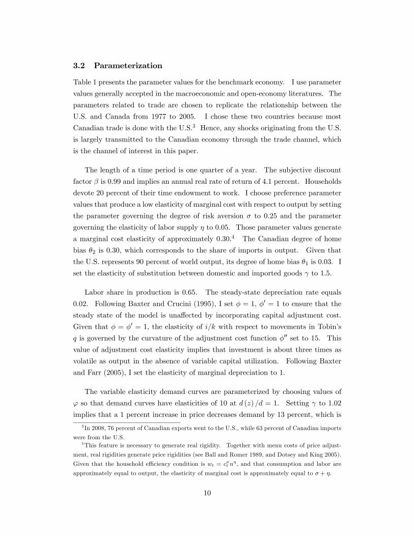
3.2 Parameterization

Table 1 presents the parameter values for the benchmark economy. I use parameter

values generally accepted in the macroeconomic and open-economy literatures. The

parameters related to trade are chosen to replicate the relationship between the

U.S. and Canada from 1977 to 2005. I chose these two countries because most

Canadian trade is done with the U.S.3 Hence, any shocks originating from the U.S.

is largely transmitted to the Canadian economy through the trade channel, which

is the channel of interest in this paper.

The length of a time period is one quarter of a year. The subjective discount

factor � is 0:99 and implies an annual real rate of return of 4:1 percent. Households

devote 20 percent of their time endowment to work. I choose preference parameter

values that produce a low elasticity of marginal cost with respect to output by setting

the parameter governing the degree of risk aversion � to 0:25 and the parameter

governing the elasticity of labor supply � to 0:05. Those parameter values generate

a marginal cost elasticity of approximately 0:30.4 The Canadian degree of home

bias �2 is 0:30, which corresponds to the share of imports in output. Given that

the U.S. represents 90 percent of world output, its degree of home bias �1 is 0:03. I

set the elasticity of substitution between domestic and imported goods to 1:5.

Labor share in production is 0:65. The steady-state depreciation rate equals

0:02. Following Baxter and Crucini (1995), I set � = 1, �0 = 1 to ensure that the

steady state of the model is una¤ected by incorporating capital adjustment cost.

Given that � = �0 = 1, the elasticity of i=k with respect to movements in Tobin�s

q is governed by the curvature of the adjustment cost function �00 set to 15. This

value of adjustment cost elasticity implies that investment is about three times as

volatile as output in the absence of variable capital utilization. Following Baxter

and Farr (2005), I set the elasticity of marginal depreciation to 1.

The variable elasticity demand curves are parameterized by choosing values of

' so that demand curves have elasticities of 10 at d (z) =d = 1. Setting to 1.02

implies that a 1 percent increase in price decreases demand by 13 percent, which is3 In 2008, 76 percent of Canadian exports went to the U.S., while 63 percent of Canadian imports

were from the U.S.4This feature is necessary to generate real rigidity. Together with menu costs of price adjust-

ment, real rigidities generate price rigidities (see Ball and Romer 1989, and Dotsey and King 2005).

Given that the household e¢ ciency condition is wt = c�t n�, and that consumption and labor are

approximately equal to output, the elasticity of marginal cost is approximately equal to � + �.

10

somewhere between the response assumed by Kimball (1995) and Bergin and Feen-

stra (2001). The remaining parameters involve the adjustment-cost distributions

which, along with the demand functions, determine the timing and distribution of

prices. Table 2 presents the steady-state adjustment hazards and vintage fractions

of adjusting �rms for each country. The adjustment-cost structure is consistent

with microeconomic data on price adjustment that suggest steady-state adjustment

hazards are quadratic in log relative price deviations (Caballero and Engle 1993).5

The parameter values imply an average age of prices of 1:75 quarters and an ex-

pected price duration of 4:05 quarters. Together, the demand and adjustment-cost

speci�cations provide a reasonable approximation of the main features governing

the pattern of price adjustments and pricing policies observed in empirical studies

such as Bils and Klenow (2004) and Nakamura and Steinsson (2008).

Money supply growth is exogenous and follows an autoregressive process of the

form

�Mi;t = �i�Mi;t�1 + "i;t for i = 1; 2, (18)

where �i represents the coe¢ cients of autocorrelation and "i;t are independently and

identically distributed zero-mean disturbances. The value of �1 is 0:53 for the U.S.

and the value of �2 is 0:42 for Canada. These values come from running a regression

on the logarithm of (18) using M1 quarterly data for the U.S. and Canada. The

standard deviation of the shocks are 1:63 percent in the U.S. and 2:94 percent in

Canada. The cross-correlations of these shocks are chosen to match two moments

observed in the data: the correlation between U.S. and Canadian output, and the

correlation between U.S. output and the U.S. trade balance. I use the simulated

method of moments to �nd the cross-correlations of these shocks. Finally, I set

the steady-state money growth rate to 4 percent, which corresponds to the average

in�ation rates observed in these countries over the sample period.

4 Findings

In this section, I �rst discuss the SDP model�s responses to the 1 percent increase

in the U.S. money stock and contrast these responses with those from a TDP model

5 I adopt the cost structure used in Dotsey and King (2005) and set the maximum adjustment

cost to 7.5 percent of household production time. This implies that the resources spent adjusting

prices relative to sales average 0.8 percent of �rms�revenues in the steady state, in line with Levy

et al. (1997).

11

for which the fractions of price-adjusting �rms are held �xed at steady-state values.

In contrast to the �at adjustment hazards of Calvo (1983), the TDP adjustment

hazards are similar to Levin (1991), in which the adjustment probabilities are con-

ditional on the amount of time elapsed since a �rm�s last price adjustment. To get

a better understanding of the mechanism through which money a¤ects international

economic activity, I start by exploring the reactions of individual �rms to a U.S.

monetary expansion in subsection 4.1. In this subsection, I also discuss the amount

of exchange rate pass-through to optimal export prices charged by price-adjusting

�rms, and to aggregate export prices. In subsection 4.2, I discuss the implications

for trade and other macroeconomic variables. Then, in subsection 4.3, I look at the

business cycle implications of the model in which the world economy experiences

shocks to U.S. and Canadian money stocks. In this subsection, I also explore the

sensitivity of my �ndings and highlight the role played by various assumptions about

the benchmark SDP model.

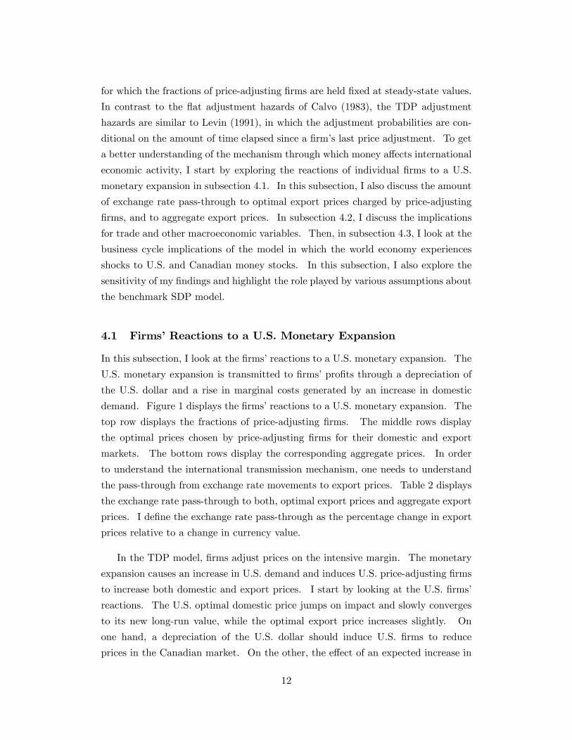
4.1 Firms�Reactions to a U.S. Monetary Expansion

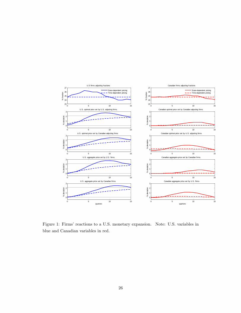
In this subsection, I look at the �rms�reactions to a U.S. monetary expansion. The

U.S. monetary expansion is transmitted to �rms�pro�ts through a depreciation of

the U.S. dollar and a rise in marginal costs generated by an increase in domestic

demand. Figure 1 displays the �rms�reactions to a U.S. monetary expansion. The

top row displays the fractions of price-adjusting �rms. The middle rows display

the optimal prices chosen by price-adjusting �rms for their domestic and export

markets. The bottom rows display the corresponding aggregate prices. In order

to understand the international transmission mechanism, one needs to understand

the pass-through from exchange rate movements to export prices. Table 2 displays

the exchange rate pass-through to both, optimal export prices and aggregate export

prices. I de�ne the exchange rate pass-through as the percentage change in export

prices relative to a change in currency value.

In the TDP model, �rms adjust prices on the intensive margin. The monetary

expansion causes an increase in U.S. demand and induces U.S. price-adjusting �rms

to increase both domestic and export prices. I start by looking at the U.S. �rms�

reactions. The U.S. optimal domestic price jumps on impact and slowly converges

to its new long-run value, while the optimal export price increases slightly. On

one hand, a depreciation of the U.S. dollar should induce U.S. �rms to reduce

prices in the Canadian market. On the other, the e¤ect of an expected increase in

12

marginal cost induces U.S. �rms to increase prices in the Canadian market. These

two e¤ects roughly balance out in a TDP environment over the expected horizon of

price rigidity. In the current framework, the latter e¤ect dominates and the optimal

export price increases little. This generates a negative exchange rate pass-through,

both in optimal and aggregate export prices.

Now, let�s turn to the behavior of the Canadian �rms. The optimal domestic

price stays near steady-state value as domestic demand remains nearly constant.

However, Canadian �rms follow their U.S. counterparts in setting U.S. prices: The

optimal export price jumps on impact and slowly converges to its new long-run

value. On impact, this generates a change in optimal export prices that is 70

percent higher than the change in currency value. This aggressive price response

diminishes over time to reach 8 percent after one year. On aggregate, the amount of

exchange rate pass-through is 35 percent on impact and 63 percent after one year.

Firms react di¤erently in the SDP model because they adjust prices on the in-

tensive and extensive margins. For the U.S. domestic market, SDP means that U.S.

�rms can make small price adjustments now knowing they can choose to increase

them later when it is more valuable to do so. Therefore, the optimal domestic price

responds little because �rms do not want to lose pro�t by raising prices too aggres-

sively. For the U.S. export market, SDP means that U.S. �rms can make bigger

pro�ts now by lowering the optimal export price. In contrast to the TDP model,

the optimal export price decreases on impact. In fact, the optimal export price

drops 15 percent more than the U.S. dollar. On aggregate, this implies an amount

of exchange rate pass-through of 28 percent. Over time, the increase in marginal

cost takes over and induces �rms to adjust prices upward. This becomes obvious

four to six quarters after the monetary expansion as the U.S. adjusting fraction and

optimal prices deviate further from their long-run values. Ultimately, the collective

action of price-adjusting �rms feeds into the aggregate price level, and the piling up

of prices and actions leads to higher optimal prices.

In turn, movements in U.S. export prices in�uence Canadian �rms�reactions. On

impact, the optimal domestic price stays near steady-state value as domestic demand

remains nearly constant, while Canadian �rms follow their U.S. counterparts in

setting U.S. prices. This generates a change in optimal export prices that is 82

percent higher than the change in currency value. As in the TDP model, this

aggressive price response diminishes over time to reach 13 percent after one year.

13

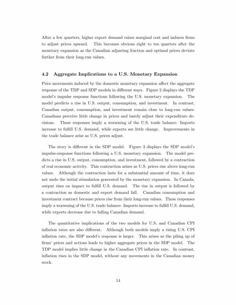
After a few quarters, higher export demand raises marginal cost and induces �rms

to adjust prices upward. This becomes obvious eight to ten quarters after the

monetary expansion as the Canadian adjusting fraction and optimal prices deviate

further from their long-run values.

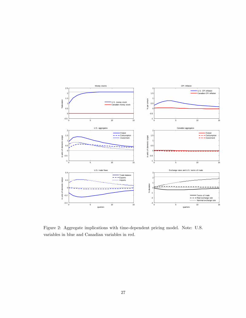
4.2 Aggregate Implications to a U.S. Monetary Expansion

Price movements induced by the domestic monetary expansion a¤ect the aggregate

response of the TDP and SDP models in di¤erent ways. Figure 2 displays the TDP

model�s impulse response functions following the U.S. monetary expansion. The

model predicts a rise in U.S. output, consumption, and investment. In contrast,

Canadian output, consumption, and investment remain close to long-run values:

Canadians perceive little change in prices and barely adjust their expenditure de-

cisions. These responses imply a worsening of the U.S. trade balance: Imports

increase to ful�ll U.S. demand, while exports see little change. Improvements in

the trade balance arise as U.S. prices adjust.

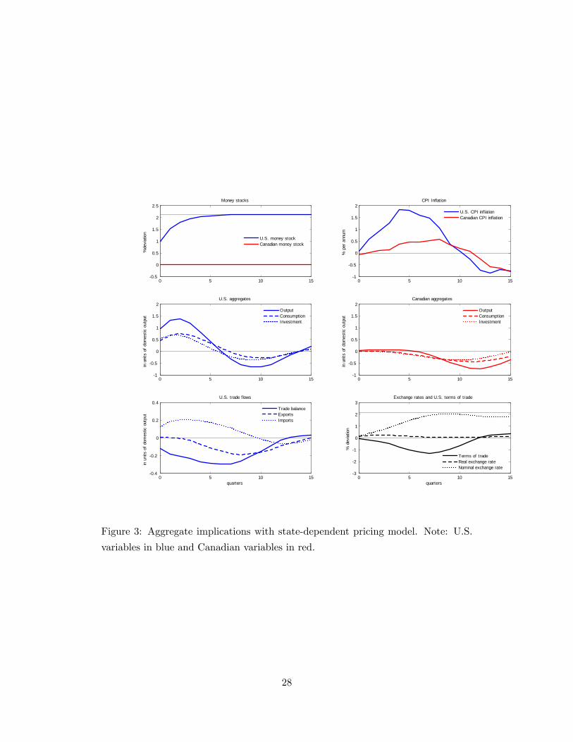
The story is di¤erent in the SDP model. Figure 3 displays the SDP model�s

impulse-response functions following a U.S. monetary expansion. The model pre-

dicts a rise in U.S. output, consumption, and investment, followed by a contraction

of real economic activity. This contraction arises as U.S. prices rise above long-run

values. Although the contraction lasts for a substantial amount of time, it does

not undo the initial stimulation generated by the monetary expansion. In Canada,

output rises on impact to ful�ll U.S. demand. The rise in output is followed by

a contraction as domestic and export demand fall. Canadian consumption and

investment contract because prices rise from their long-run values. These responses

imply a worsening of the U.S. trade balance: Imports increase to ful�ll U.S. demand,

while exports decrease due to falling Canadian demand.

The quantitative implications of the two models for U.S. and Canadian CPI

in�ation rates are also di¤erent. Although both models imply a rising U.S. CPI

in�ation rate, the SDP model�s response is larger. This arises as the piling up of

�rms�prices and actions leads to higher aggregate prices in the SDP model. The

TDP model implies little change in the Canadian CPI in�ation rate. In contrast,

in�ation rises in the SDP model, without any movements in the Canadian money

stock.

14

4.3 Business Cycles Analysis

In this subsection, I look at the business cycle implications of the model. First,

I discuss the main features of U.S. and Canadian economic �uctuations as well as

trade between the two countries. Second, I take the model to the data by assuming

that both countries�money stocks evolve over the business cycle. Finally, I examine

the sensitivity of my �ndings by varying assumptions about the benchmark features.

4.3.1 The Data

The U.S. data are from the Bureau of Economic Analysis, with the exception of the

monetary aggregate and the quarterly exchange rates, which are from the Board of

Governors of the Federal Reserve System. The Canadian data are from Statistics

Canada, with the exception of the monetary aggregate, which is from the Bank of

Canada. Appendix A o¤ers a more detailed description of the data.

Table 4 presents the business cycle statistics for output, consumption, invest-

ment, trade balances, and CPI in�ation rates for the U.S. and Canada. The trade

balances include only trade between the two countries and are relative to output.

Table 5 presents the business cycle statistics for real and nominal exchange rates,

as well as for the CPI price ratio. The moments were calculated using a band-pass

business-cycle �lter that admits frequency components between 6 and 32 quarters.

Although the data are from 1974Q1 to 2008Q4, the e¤ective data used in the band-

pass statistics are from 1977Q1 to 2005Q4 (see Baxter and King 1999). All the

variables were de�ated using the implicit price de�ators for gross domestic product.

Output, consumption, and investment are procyclical, with consumption being

less volatile than output and investment being more volatile than output. The

U.S. trade balance is countercyclical, but the Canadian trade balance is procyclical.

Both have a volatility much lower than output. CPI in�ation rates are procyclical

and have a volatility much lower than output. The correlations between U.S. and

Canadian output, consumption, investment, and CPI in�ation rates are all positive.

As for international prices, real and nominal exchange rates are highly correlated

and highly volatile relative to output. The CPI price ratio is positively correlated

with the real exchange rate and about half as volatile as output.

15

4.3.2 The Benchmark Models

Tables 4 and 5 present the �ltered moments generated by the SDP and TDP models.

I assume that both countries�money stocks evolve over the business cycle and that

these shocks are the only exogenous shocks in the model.6 For each model, the cross-

correlations of the monetary shocks are set to reproduce the correlation between U.S.

and Canadian output and the correlation between U.S. output and the U.S. trade

balance observed in the data.

The SDP model performs well in terms of predictions for relative volatility,

autocorrelation, and correlation with output. In the TDP model, the correlation

between Canadian output and the trade balance has the wrong sign, and the corre-

lation between Canadian output and the CPI in�ation rate is too strong. Finally,

both models capture the positive cross-country correlations of output, consump-

tion, investment, and CPI in�ation rates�although the consumption and investment

cross-country correlations are higher than the output cross-country correlation in

the SDP model.

As for international prices, the relative volatilities of the real and nominal ex-

change rates with respect to output are too small in both models. The SDP model

also predicts a negative correlation between the real and nominal exchange rate,

which is contrary to the data. However, the SDP model does a good job matching

the dynamics of the CPI price ratio�it does particularly well matching the volatility

of this ratio relative to U.S. output and its correlation relative to the real exchange

rate.

4.3.3 Variations on the Benchmark SDP Model

Finally, I examine the sensitivity of my �ndings by varying assumptions about three

of the SDP model�s features. Tables 4 and 5 present the business-cycle moments

under the three alternative scenarios: an economy with Dixit-Stiglitz demands (' =

0), an economy without variable capital utilization (but keeping investment), and

an economy with a single uncontingent nominal bond.

6Technology and other types of shocks are important sources of business cycles. However, many

papers in the literature, notably Chari et al. (2002), compare their model�s moments to those of

the data, with movements in money stocks as the only source of exogenous shocks. Thus, I provide

this comparison for my own models as a way to compare my results with those in the literature.

16

The variants with Dixit-Stiglitz demands and without variable capital utilization

are able to generate a lower cross-country consumption correlation but perform worst

in many other dimensions, notably in terms of CPI in�ation rates and trade balance

dynamics. As for international prices, the correlation between the real exchange rate

and the price ratio has the wrong sign in the variant with Dixit-Stiglitz demands.

Finally, the performance of the variant with a single uncontingent nominal bond is

roughly similar to the SDP model benchmark with complete �nancial markets.

5 Conclusion

This paper developed a two-country model with SDP in which �rms price-discriminate

across countries by setting prices in the local currency. I show that a domestic mon-

etary expansion has greater spillover e¤ects to foreign prices and foreign economic

activity than an otherwise identical model with TDP. The spillover e¤ects arise

because of the interplay between the intensive and extensive margins. This result

suggests that the monetary policy implications associated with local-currency pric-

ing are probably speci�c to the TDP speci�cations. Next, I look at the implications

of the business-cycle moments generated by the models and compared them with

moments generated by the data. I �nd that the SDP model�s predictions match

the business-cycle moments better than the predictions of the TDP model.

Unfortunately, the SDP model has two caveats relative to other TDP models in

the literature. First, by breaking the ability of local-currency pricing to insulate the

foreign economy from a domestic monetary shock, the SDP benchmark model loses

the ability to generate low cross-country consumption and investment correlations.

Second, the SDP model is unable to replicate the dynamics between the real and

nominal exchange rates observed in the data. Adding frictions to �x these two

caveats is something to investigate in future research.

17

A Data

The data cover the period 1974Q1 to 2008Q4. U.S. data from the Bureau of Eco-

nomic Analysis are the implicit price de�ators for gross domestic product and for

private consumption. Gross domestic product, private consumption expenditures,

private �xed investment, and exports and imports of goods and services to/from

Canada are seasonally adjusted and in billions of U.S. dollars. Canadian data from

Statistics Canada are the implicit price de�ators for gross domestic product and for

private consumption. Gross domestic product, personal consumption expenditures,

and business �xed investment are seasonally adjusted and in millions of Canadian

dollars. Quarterly averages of the nominal exchange rate and the U.S. monetary ag-

gregate M1, nonseasonally adjusted, are from the Board of Governors of the Federal

Reserve System. The Canadian monetary aggregate M1, nonseasonally adjusted,

is from the Bank of Canada. Canadian exports and imports of goods and services

to/from the U.S. are from the Bureau of Economic Analysis, converted to Canadian

dollars using the quarterly nominal exchange rate.

18

References

[1] Ball, L. and Romer, D., 1990. Real Rigidities and the Non-Neutrality of Money.

Review of Economic Studies 57, 183-203.

[2] Baxter, M. and Crucini, M. J., 1993. Explaining Saving-Investment Correla-

tions. American Economic Review 83, 416-436.

[3] Baxter, M., and Farr, D. D., 2005. Variable Capital Utilization and Interna-

tional Business Cycles. Journal of International Economics 65, 335-347.

[4] Baxter, M., and King, R.G., 1999. Measuring Business Cycles: Approximate

Band-Pass Filters for Macroeconomic Time Series. Review of Economics and

Statistics 81, 575-593.

[5] Bergin, P., and Feenstra, R. C., 2001. Pricing-to-Market, Staggered Contracts,

and Real Exchange Rate Persistance. Journal of International Economics 54,

333-359.

[6] Betts, C., and Devereux, M.B., 2000. Exchange Rate Dynamics in a Model of

Pricing-to-Market. Journal of International Economics 50, 215-244.

[7] Bils, M., and Klenow, P., 2004. Some Evidence on the Importance of Sticky

Prices. Journal of Political Economy 112, 947-985.

[8] Bouakez, H., 2005. Nominal Rigidity, Desired Markup Variations, and Real

Exchange Rate Persistence. Journal of International Economics 66, 49-74.

[9] Caballero, R., and Engle, E., 1993. Microeconomics Rigidities and Aggregate

Price Dynamics. European Economic Review 37, 697-717.

[10] Calvo, G., 1983. Staggered Prices in a Utility-Maximizing Framework. Journal

of Monetary Economics 12, 383-398.

[11] Chari, V.V., Kehoe, P.J., and McGrattan, E.R., 2002. Can Sticky Price Models

Generate Volatile and Persistent Real Exchange Rates? Review of Economic

Studies 69, 533-564.

[12] Dotsey, M., and King, R.G., 2005. Implication of State-Dependent Pricing for

Dynamic Macroeconomic Models. Journal of Monetary Economics - Carnegie-

Rochester Series on Public Policy 52, 213-242.

19

[13] Dotsey, M., King, R.G., and Wolman, A.L., 1999. State-Dependent Pricing and

the General Equilibrium Dynamics of Money and Output. Quarterly Journal

of Economics 114, 655-690.

[14] Floden, M. and Wilander, F., 2006. State-Dependent Pricing, Invoicing Cur-

rency, and Exchange Rate Pass-Through. Journal of International Economics

70, 178-196.

[15] Gopinath, G., Itskhoki, O, and Rigobon, R., 2009. Currency Choice and Ex-

change Rate Pass-Through. American Economic Review, forthcoming.

[16] Gopinath, G., and Itskhoki, O., 2009. Frequency of Price Adjustment and Pass-

Through. Quarterly Journal of Economics, forthcoming.

[17] Gust, C., Leduc, S., and Vigfusson, R.J., 2006. Trade Integration, Competi-

tion, and the Decline in Exchange-Rate Pass-Through. International Finance

Discussion Paper 864.

[18] Kimball, M.S., 1995. The Quantitative Analytics of the Basis Neomonetarist

Model. Journal of Money, Credit, and Banking 27, 1241-1277.

[19] King, R.G., and Watson, M.W., 1998. The Solution of Singular Linear Di¤er-

ence Systems Under Rational Expectations. International Economic Review 39,

1015-1026.

[20] Kollmann, R., 2001. The Exchange Rate in a Dynamic-Optimizing Business

Cycle Model with Nominal Rigidities: A Quantitative Investigation. Journal of

International Economics, 243-262.

[21] Landry, A., 2009. Expectation and Exchange-Rate Dynamics: A State-

Dependent Pricing Approach. Journal of International Economics 78, 60-71.

[22] Levin, A., 1991. The Macroeconomic Signi�cance of Nominal Wage Contract

Duration. Discussion paper 91-08, University of California at San Diego.

[23] Levy, D., Bergen, M., Dutta, S., and Venable, S., 1997. The Magnitude of

Menu Costs: Direct Evidence from a Large U.S. Supermarket Chain. Quarterly

Journal of Economics 112, 791-825.

[24] Nakamura, E., and Steinsson, J., 2008. Five Facts About Prices: A Reevalua-

tion of the Menu Cost Models. Quarterly Journal of Economics 123, 1415-1464.

20

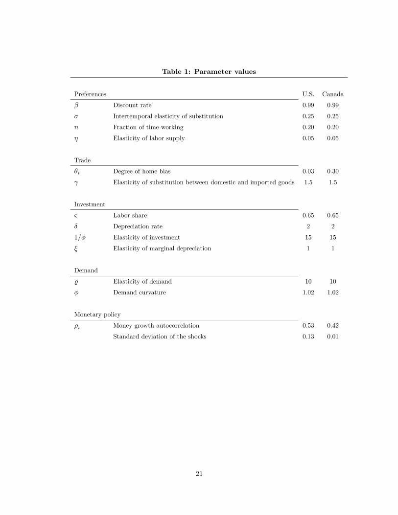
Table 1: Parameter values

Preferences U.S. Canada

� Discount rate 0.99 0.99

� Intertemporal elasticity of substitution 0.25 0.25

n Fraction of time working 0.20 0.20

� Elasticity of labor supply 0.05 0.05

Trade

�i Degree of home bias 0.03 0.30

Elasticity of substitution between domestic and imported goods 1.5 1.5

Investment

& Labor share 0.65 0.65

� Depreciation rate 2 2

1=� Elasticity of investment 15 15

� Elasticity of marginal depreciation 1 1

Demand

% Elasticity of demand 10 10

� Demand curvature 1.02 1.02

Monetary policy

�i Money growth autocorrelation 0.53 0.42

Standard deviation of the shocks 0.13 0.01

21

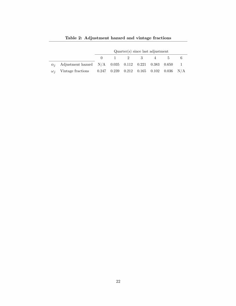
Table 2: Adjustment hazard and vintage fractions

Quarter(s) since last adjustment

0 1 2 3 4 5 6

�j Adjustment hazard N/A 0.035 0.112 0.221 0.383 0.650 1

!j Vintage fractions 0.247 0.239 0.212 0.165 0.102 0.036 N/A

22

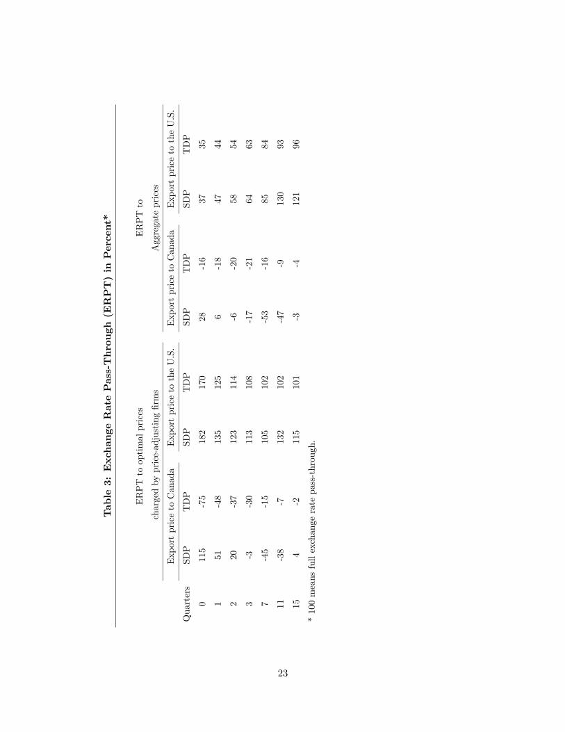
Table3:ExchangeRatePass-Through

(ERPT)inPercent*

ERPTtooptimalprices

ERPTto

chargedbyprice-adjusting�rms

Aggregateprices

ExportpricetoCanada

ExportpricetotheU.S.

ExportpricetoCanada

ExportpricetotheU.S.

Quarters

SDP

TDP

SDP

TDP

SDP

TDP

SDP

TDP

0115

-75

182

170

28-16

3735

151

-48

135

125

6-18

4744

220

-37

123

114

-6-20

5854

3-3

-30

113

108

-17

-21

6463

7-45

-15

105

102

-53

-16

8584

11-38

-7132

102

-47

-9130

93

154

-2115

101

-3-4

121

96

*100meansfullexchangeratepass-through.

23

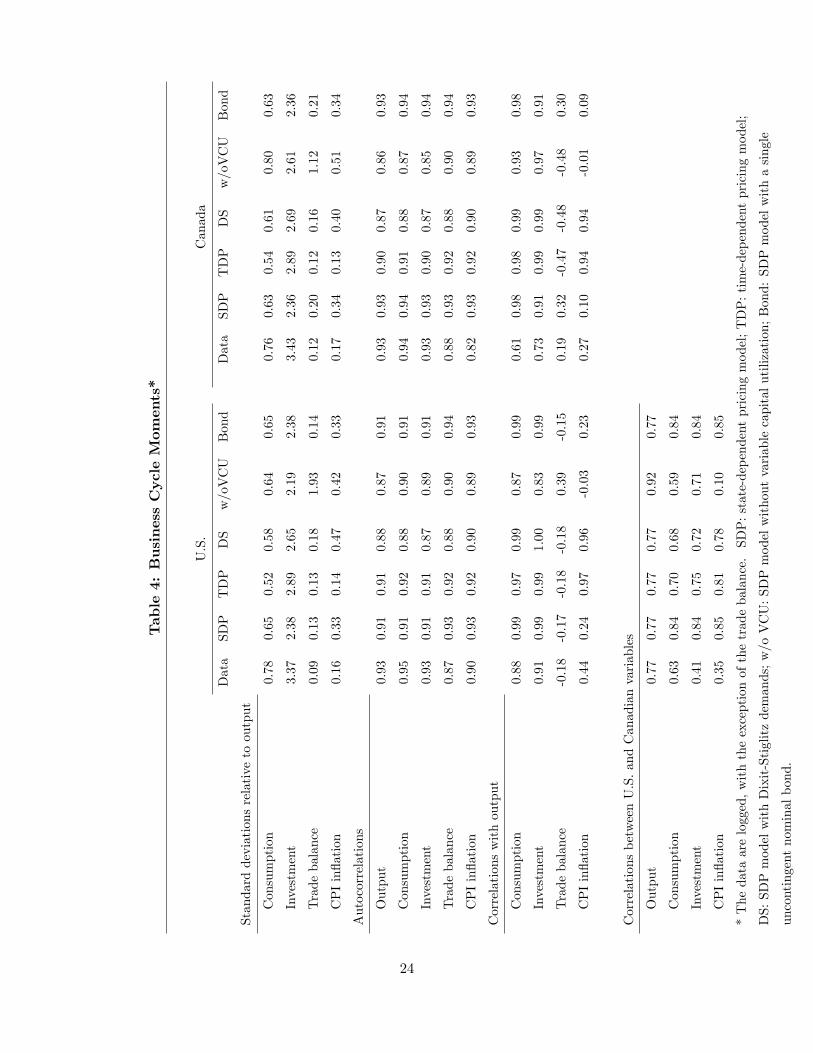
Table4:BusinessCycleMom

ents*

U.S.

Canada

Data

SDP

TDP

DS

w/oVCU

Bond

Data

SDP

TDP

DS

w/oVCU

Bond

Standarddeviationsrelativetooutput

Consumption

0.78

0.65

0.52

0.58

0.64

0.65

0.76

0.63

0.54

0.61

0.80

0.63

Investment

3.37

2.38

2.89

2.65

2.19

2.38

3.43

2.36

2.89

2.69

2.61

2.36

Tradebalance

0.09

0.13

0.13

0.18

1.93

0.14

0.12

0.20

0.12

0.16

1.12

0.21

CPIin�ation

0.16

0.33

0.14

0.47

0.42

0.33

0.17

0.34

0.13

0.40

0.51

0.34

Autocorrelations

Output

0.93

0.91

0.91

0.88

0.87

0.91

0.93

0.93

0.90

0.87

0.86

0.93

Consumption

0.95

0.91

0.92

0.88

0.90

0.91

0.94

0.94

0.91

0.88

0.87

0.94

Investment

0.93

0.91

0.91

0.87

0.89

0.91

0.93

0.93

0.90

0.87

0.85

0.94

Tradebalance

0.87

0.93

0.92

0.88

0.90

0.94

0.88

0.93

0.92

0.88

0.90

0.94

CPIin�ation

0.90

0.93

0.92

0.90

0.89

0.93

0.82

0.93

0.92

0.90

0.89

0.93

Correlationswithoutput

Consumption

0.88

0.99

0.97

0.99

0.87

0.99

0.61

0.98

0.98

0.99

0.93

0.98

Investment

0.91

0.99

0.99

1.00

0.83

0.99

0.73

0.91

0.99

0.99

0.97

0.91

Tradebalance

-0.18

-0.17

-0.18

-0.18

0.39

-0.15

0.19

0.32

-0.47

-0.48

-0.48

0.30

CPIin�ation

0.44

0.24

0.97

0.96

-0.03

0.23

0.27

0.10

0.94

0.94

-0.01

0.09

CorrelationsbetweenU.S.andCanadianvariables

Output

0.77

0.77

0.77

0.77

0.92

0.77

Consumption

0.63

0.84

0.70

0.68

0.59

0.84

Investment

0.41

0.84

0.75

0.72

0.71

0.84

CPIin�ation

0.35

0.85

0.81

0.78

0.10

0.85

*Thedataarelogged,withtheexceptionofthetradebalance.SDP:state-dependentpricingmodel;TDP:time-dependentpricingmodel;

DS:SDPmodelwithDixit-Stiglitzdemands;w/oVCU:SDPmodelwithoutvariablecapitalutilization;Bond:SDPmodelwithasingle

uncontingentnominalbond.

24

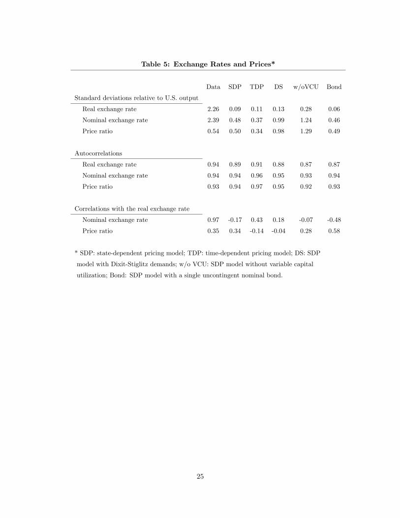
Table 5: Exchange Rates and Prices*

Data SDP TDP DS w/oVCU Bond

Standard deviations relative to U.S. output

Real exchange rate 2.26 0.09 0.11 0.13 0.28 0.06

Nominal exchange rate 2.39 0.48 0.37 0.99 1.24 0.46

Price ratio 0.54 0.50 0.34 0.98 1.29 0.49

Autocorrelations

Real exchange rate 0.94 0.89 0.91 0.88 0.87 0.87

Nominal exchange rate 0.94 0.94 0.96 0.95 0.93 0.94

Price ratio 0.93 0.94 0.97 0.95 0.92 0.93

Correlations with the real exchange rate

Nominal exchange rate 0.97 -0.17 0.43 0.18 -0.07 -0.48

Price ratio 0.35 0.34 -0.14 -0.04 0.28 0.58

* SDP: state-dependent pricing model; TDP: time-dependent pricing model; DS: SDP

model with Dixit-Stiglitz demands; w/o VCU: SDP model without variable capital

utilization; Bond: SDP model with a single uncontingent nominal bond.

25

0 5 10 1523

24

25

26

27U.S firms adjusting fractions

% f

ract

ion

State­dependent pricingTime­dependent pricing

0 5 10 1523

24

25

26

27Canadian firms adjusting fractions

% f

ract

ion

State­dependent pricingTime­dependent pricing

0 5 10 15

0

1

2

3U.S. optimal price set by U.S. adjusting firms

% d

eviat

ion

0 5 10 15

0

1

2

3Canadian optimal price set by Canadian adjusting firms

% d

eviat

ion

0 5 10 15

0

1

2

3U.S. optimal price set by Canadian adjusting firms

% d

eviat

ion

0 5 10 15

0

1

2

3Canadian optimal price set by U.S. adjusting firms

% d

eviat

ion

0 5 10 15

0

1

2

3U.S. aggregate price set by U.S. firms

% d

eviat

ion

0 5 10 15

0

1

2

3Canadian aggregate price set by Canadian firms

% d

eviat

ion

0 5 10 15

0

1

2

3U.S. aggregate price set by Canadian firms

% d

eviat

ion

quarters0 5 10 15

0

1

2

3Canadian aggregate price set by U.S. firms

% d

eviat

ion

quarters

Figure 1: Firms�reactions to a U.S. monetary expansion. Note: U.S. variables in

blue and Canadian variables in red.

26

0 5 10 15­0.5

0

0.5

1

1.5

2

2.5

%de

viat

ion

Money stocks

U.S. money stockCanadian money stock

0 5 10 15­1

­0.5

0

0.5

1

1.5

2CPI Inflation

% p

er a

nnum

U.S. CPI inflationCanadian CPI inflation

0 5 10 15­1

­0.5

0

0.5

1

1.5

2U.S. aggregates

in u

nits

 of 

dom

estic

 out

put

OutputConsumptionInvestment

0 5 10 15­1

­0.5

0

0.5

1

1.5

2Canadian aggregates

in u

nits

 of 

dom

estic

 out

put

OutputConsumptionInvestment

0 5 10 15­0.4

­0.2

0

0.2

0.4U.S. trade flows

quarters

in u

nits

 of 

dom

estic

 out

put

Trade balanceExportsImports

0 5 10 15­3

­2

­1

0

1

2

3Exchange rates and U.S. terms of trade

quarters

% d

eviat

ion

Terms of tradeReal exchange rateNominal exchange rate

Figure 2: Aggregate implications with time-dependent pricing model. Note: U.S.

variables in blue and Canadian variables in red.

27

0 5 10 15­0.5

0

0.5

1

1.5

2

2.5

%de

viat

ion

Money stocks

U.S. money stockCanadian money stock

0 5 10 15­1

­0.5

0

0.5

1

1.5

2CPI Inflation

% p

er a

nnum

U.S. CPI inflationCanadian CPI inflation

0 5 10 15­1

­0.5

0

0.5

1

1.5

2U.S. aggregates

in u

nits

 of 

dom

estic

 out

put

OutputConsumptionInvestment

0 5 10 15­1

­0.5

0

0.5

1

1.5

2Canadian aggregates

in u

nits

 of 

dom

estic

 out

put

OutputConsumptionInvestment

0 5 10 15­0.4

­0.2

0

0.2

0.4U.S. trade flows

quarters

in u

nits

 of 

dom

estic

 out

put

Trade balanceExportsImports

0 5 10 15­3

­2

­1

0

1

2

3Exchange rates and U.S. terms of trade

quarters

% d

eviat

ion

Terms of tradeReal exchange rateNominal exchange rate

Figure 3: Aggregate implications with state-dependent pricing model. Note: U.S.

variables in blue and Canadian variables in red.

28