state space modelling - accueil - cel
TRANSCRIPT

HAL Id: hal-02987750https://cel.archives-ouvertes.fr/hal-02987750v2
Submitted on 12 Jan 2021
HAL is a multi-disciplinary open accessarchive for the deposit and dissemination of sci-entific research documents, whether they are pub-lished or not. The documents may come fromteaching and research institutions in France orabroad, or from public or private research centers.
L’archive ouverte pluridisciplinaire HAL, estdestinée au dépôt et à la diffusion de documentsscientifiques de niveau recherche, publiés ou non,émanant des établissements d’enseignement et derecherche français ou étrangers, des laboratoirespublics ou privés.
Distributed under a Creative Commons Attribution - NonCommercial| 4.0 InternationalLicense
State Space ModellingThierry Miquel
To cite this version:
Thierry Miquel. State Space Modelling. Master. ENAC, France. 2021. hal-02987750v2


2

Course overview
Classical control theory is intrinsically linked to the frequency domain and thes-plane. The main drawback of classical control theory is the diculty toapply it in Multi-Input Multi-Output (MIMO) systems. Rudolf Emil Kalman(Hungarian-born American, May 19, 1930 July 2, 2016) is one of the greatestprotagonist of modern control theory1. He has introduced the concept of stateas well as linear algebra and matrices in control theory. With this formalismsystems with multiple inputs and outputs could easily be treated.
The purpose of this lecture is to present an overview of modern controltheory. More specically, the objectives are the following:
− to learn how to model dynamic systems in the state-space and the state-space representation of transfer functions;
− to learn linear dynamical systems analysis in state-space: more specicallyto solve the time invariant state equation and to get some insight oncontrollability, observability and stability;
− to learn state-space methods for observers and controllers design.
Assumed knowledge encompass linear algebra, Laplace transform and linearordinary dierential equations (ODE)
This lecture is organized as follows:
− The rst chapter focuses on the state-space representation as well as state-space representation associated to system interconnection;
− The conversion from transfer functions to state-space representation ispresented in the second chapter. This is also called transfer functionrealization;
− The analysis of linear dynamical systems is presented in the third chapter;more specically we will concentrate on the solution of the state equationand present the notions of controllability, observability and stability;
− The fourth chapter is dedicated to observers design. This chapter focuseson Luenberger observer, state observer for SISO systems in observablecanonical form, state observer for SISO systems in arbitrary state-spacerepresentation and state observer for MIMO systems will be presented.
1http://www.uta.edu/utari/acs/history.htm

4
− The fth chapter is dedicated to observers and controllers design. As faras observers and controllers are linked through the duality principle theframe of this chapter will be similar to the previous chapter: state feedbackcontroller for SISO systems in controllable canonical form, state feedbackcontroller for SISO systems in arbitrary state-space representation, staticstate feedback controller and static output feedback controller for MIMOsystems will be presented.

References
[1] Modern Control Systems, Richard C. Dorf, Robert H. Bishop,Prentice Hall
[2] Feedback Control of Dynamic Systems, Gene F. Franklin, J Powel,Abbas Emami-Naeini, Pearson
[3] Linear Control System Analysis and Design, Constantine H.Houpis, Stuart N. Sheldon, John J. D'Azzo, CRC Press
[4] Modern Control Engineering, P.N. Paraskevopoulos, CRC Press
[5] Control Engineering: An Introductory Course, Michael Johnson,Jacqueline Wilkie, Palgrave Macmillan
[6] Control Engineering: A Modern Approach, P. Bélanger, OxfordUniversity Press
[7] Multivariable Feedback Control Analysis and design, S. Skogestadand I. Postlethwaite, Wiley

6 References

Table of contents
1 State-space representation 11
1.1 Introduction . . . . . . . . . . . . . . . . . . . . . . . . . . . . . . 11
1.2 State and output equations . . . . . . . . . . . . . . . . . . . . . 12
1.3 From ordinary dierential equations to state-space representation 14
1.3.1 Brunovsky's canonical form . . . . . . . . . . . . . . . . . 14
1.3.2 Linearization of non-linear time-invariant state-spacerepresentation . . . . . . . . . . . . . . . . . . . . . . . . . 15
1.4 From state-space representation to transfer function . . . . . . . 21
1.5 Zeros of a transfer function - Rosenbrock's system matrix . . . . 23
1.6 Faddeev-Leverrier's method to compute (sI−A)−1 . . . . . . . . 25
1.7 Matrix inversion lemma . . . . . . . . . . . . . . . . . . . . . . . 28
1.8 Interconnection of systems . . . . . . . . . . . . . . . . . . . . . . 29
1.8.1 Parallel interconnection . . . . . . . . . . . . . . . . . . . 29
1.8.2 Series interconnection . . . . . . . . . . . . . . . . . . . . 30
1.8.3 Feedback interconnection . . . . . . . . . . . . . . . . . . 31
2 Realization of transfer functions 33
2.1 Introduction . . . . . . . . . . . . . . . . . . . . . . . . . . . . . . 33
2.2 Non-unicity of state-space representation . . . . . . . . . . . . . . 33
2.2.1 Similarity transformations . . . . . . . . . . . . . . . . . . 33
2.2.2 Inverse of a similarity transformation . . . . . . . . . . . . 35
2.3 Realization of SISO transfer function . . . . . . . . . . . . . . . . 35
2.3.1 Controllable canonical form . . . . . . . . . . . . . . . . . 36
2.3.2 Poles and zeros of the transfer function . . . . . . . . . . . 39
2.3.3 Similarity transformation to controllable canonical form . 39
2.3.4 Observable canonical form . . . . . . . . . . . . . . . . . . 46
2.3.5 Similarity transformation to observable canonical form . . 49
2.3.6 Diagonal (or modal) form . . . . . . . . . . . . . . . . . . 56
2.3.7 Algebraic and geometric multiplicity of an eigenvalue . . . 63
2.3.8 Jordan form and generalized eigenvectors . . . . . . . . . 64
2.4 Realization of SIMO transfer function . . . . . . . . . . . . . . . 70
2.4.1 Generic procedure . . . . . . . . . . . . . . . . . . . . . . 70
2.4.2 Controllable canonical form . . . . . . . . . . . . . . . . . 72
2.5 Realization of MIMO transfer function . . . . . . . . . . . . . . . 75
2.5.1 Generic procedure . . . . . . . . . . . . . . . . . . . . . . 75
2.5.2 Controllable canonical form . . . . . . . . . . . . . . . . . 77

8 Table of contents
2.5.3 Diagonal (or modal) form . . . . . . . . . . . . . . . . . . 78
2.6 Minimal realization . . . . . . . . . . . . . . . . . . . . . . . . . . 81
2.6.1 System's dimension . . . . . . . . . . . . . . . . . . . . . . 81
2.6.2 Gilbert's minimal realization . . . . . . . . . . . . . . . . 84
2.6.3 Ho-Kalman algorithm . . . . . . . . . . . . . . . . . . . . 85
3 Analysis of Linear Time Invariant systems 87
3.1 Introduction . . . . . . . . . . . . . . . . . . . . . . . . . . . . . . 87
3.2 Solving the time invariant state equation . . . . . . . . . . . . . . 87
3.3 Output response . . . . . . . . . . . . . . . . . . . . . . . . . . . 89
3.4 Impulse and unit step responses . . . . . . . . . . . . . . . . . . . 89
3.5 Matrix exponential . . . . . . . . . . . . . . . . . . . . . . . . . . 90
3.5.1 Denition . . . . . . . . . . . . . . . . . . . . . . . . . . . 90
3.5.2 Properties . . . . . . . . . . . . . . . . . . . . . . . . . . . 92
3.5.3 Computation of eAt thanks to the diagonal form of A . . 93
3.5.4 Computation of eAt thanks to the Laplace transform . . . 97
3.6 Stability . . . . . . . . . . . . . . . . . . . . . . . . . . . . . . . . 101
3.7 Controllability . . . . . . . . . . . . . . . . . . . . . . . . . . . . 103
3.7.1 Denition . . . . . . . . . . . . . . . . . . . . . . . . . . . 103
3.7.2 Use of the diagonal form: Gilbert's criteria . . . . . . . . 104
3.7.3 Popov-Belevitch-Hautus (PBH) test . . . . . . . . . . . . 105
3.7.4 Kalman's controllability rank condition . . . . . . . . . . 106
3.7.5 Uncontrollable mode . . . . . . . . . . . . . . . . . . . . . 108
3.7.6 Stabilizability . . . . . . . . . . . . . . . . . . . . . . . . . 110
3.8 Observability . . . . . . . . . . . . . . . . . . . . . . . . . . . . . 110
3.8.1 Denition . . . . . . . . . . . . . . . . . . . . . . . . . . . 110
3.8.2 Use of the diagonal form: Gilbert's criteria . . . . . . . . 111
3.8.3 Popov-Belevitch-Hautus (PBH) test . . . . . . . . . . . . 112
3.8.4 Kalman's observability rank condition . . . . . . . . . . . 113
3.8.5 Unobservable mode . . . . . . . . . . . . . . . . . . . . . . 115
3.8.6 Detectability . . . . . . . . . . . . . . . . . . . . . . . . . 115
3.9 Interpretation of the diagonal (or modal) decomposition . . . . . 115
3.10 Duality principle . . . . . . . . . . . . . . . . . . . . . . . . . . . 118
3.11 Kalman decomposition . . . . . . . . . . . . . . . . . . . . . . . . 118
3.11.1 Controllable / uncontrollable decomposition . . . . . . . . 118
3.11.2 Observable / unobservable decomposition . . . . . . . . . 119
3.11.3 Canonical decomposition . . . . . . . . . . . . . . . . . . . 120
3.12 Minimal realization (again!) . . . . . . . . . . . . . . . . . . . . . 124
4 Observer design 125
4.1 Introduction . . . . . . . . . . . . . . . . . . . . . . . . . . . . . . 125
4.2 Luenberger observer . . . . . . . . . . . . . . . . . . . . . . . . . 126
4.3 State observer for SISO systems in observable canonical form . . 128
4.4 State observer for SISO systems in arbitrary state-spacerepresentation . . . . . . . . . . . . . . . . . . . . . . . . . . . . . 130
4.5 Ackermann's formula . . . . . . . . . . . . . . . . . . . . . . . . . 132
4.6 State observer for MIMO systems - Roppenecker's formula . . . . 134

Table of contents 9
4.7 Reduced-order observer . . . . . . . . . . . . . . . . . . . . . . . 138
5 Controller design 141
5.1 Introduction . . . . . . . . . . . . . . . . . . . . . . . . . . . . . . 141
5.2 Static state feedback controller . . . . . . . . . . . . . . . . . . . 141
5.3 Control of SISO systems . . . . . . . . . . . . . . . . . . . . . . . 143
5.3.1 State feedback controller in controllable canonical form . . 143
5.3.2 State feedback controller in arbitrary state-spacerepresentation . . . . . . . . . . . . . . . . . . . . . . . . . 144
5.3.3 Ackermann's formula . . . . . . . . . . . . . . . . . . . . . 146
5.3.4 Zeros of closed-loop transfer function . . . . . . . . . . . . 149
5.4 Observer-based controller . . . . . . . . . . . . . . . . . . . . . . 149
5.4.1 Separation principle . . . . . . . . . . . . . . . . . . . . . 149
5.4.2 Example . . . . . . . . . . . . . . . . . . . . . . . . . . . . 151
5.4.3 Transfer function . . . . . . . . . . . . . . . . . . . . . . . 153
5.4.4 Algebraic controller design . . . . . . . . . . . . . . . . . . 153
5.5 Control of MIMO systems . . . . . . . . . . . . . . . . . . . . . . 155
5.5.1 Frequency domain approach for state feedback . . . . . . 155
5.5.2 Invariance of (transmission) zeros under state feedback . . 157
5.6 Pre-ltering applied to SISO plants . . . . . . . . . . . . . . . . . 157
5.7 Control with integral action . . . . . . . . . . . . . . . . . . . . . 159
5.7.1 Roppenecker's formula . . . . . . . . . . . . . . . . . . . . 160
5.8 Solving general algebraic Riccati and Lyapunov equations . . . . 165
5.9 Static output feedback . . . . . . . . . . . . . . . . . . . . . . . . 167
5.9.1 Partial eigenvalues assignment . . . . . . . . . . . . . . . 167
5.9.2 Changing PID controller into static output feedback . . . 170
5.9.3 Adding integrators, controllability and observability indexes172
5.10 Mode decoupling . . . . . . . . . . . . . . . . . . . . . . . . . . . 173
5.10.1 Input-output decoupling . . . . . . . . . . . . . . . . . . . 173
5.10.2 Eigenstructure assignment . . . . . . . . . . . . . . . . . . 175
5.10.3 Design procedure . . . . . . . . . . . . . . . . . . . . . . . 177
5.10.4 Example . . . . . . . . . . . . . . . . . . . . . . . . . . . . 181
5.11 Dynamical output feedback control . . . . . . . . . . . . . . . . . 184
5.11.1 From dynamical output feedback to observer-based control 184
5.11.2 Dynamic compensator for pole placement . . . . . . . . . 185
5.11.3 Dynamical output feedback . . . . . . . . . . . . . . . . . 186
5.12 Sensitivity to additive uncertainties . . . . . . . . . . . . . . . . . 189
Appendices 193
A Refresher on linear algebra 195
A.1 Section overview . . . . . . . . . . . . . . . . . . . . . . . . . . . 195
A.2 Vectors . . . . . . . . . . . . . . . . . . . . . . . . . . . . . . . . 195
A.2.1 Denitions . . . . . . . . . . . . . . . . . . . . . . . . . . 195
A.2.2 Vectors operations . . . . . . . . . . . . . . . . . . . . . . 196
A.3 Matrices . . . . . . . . . . . . . . . . . . . . . . . . . . . . . . . . 197
A.3.1 Denitions . . . . . . . . . . . . . . . . . . . . . . . . . . 197

10 Table of contents
A.3.2 Matrix Operations . . . . . . . . . . . . . . . . . . . . . . 198A.3.3 Properties . . . . . . . . . . . . . . . . . . . . . . . . . . . 199A.3.4 Determinant and inverse . . . . . . . . . . . . . . . . . . . 199
A.4 Eigenvalues and eigenvectors . . . . . . . . . . . . . . . . . . . . 200
B Overview of Lagrangian Mechanics 203
B.1 Euler-Lagrange equations . . . . . . . . . . . . . . . . . . . . . . 203B.2 Robot arm . . . . . . . . . . . . . . . . . . . . . . . . . . . . . . . 206B.3 Quadrotor . . . . . . . . . . . . . . . . . . . . . . . . . . . . . . . 208
B.3.1 Inertial frame and body frame . . . . . . . . . . . . . . . . 208B.3.2 Kinematic relationships . . . . . . . . . . . . . . . . . . . 209B.3.3 Forces and torques . . . . . . . . . . . . . . . . . . . . . . 210B.3.4 Generalized coordinates . . . . . . . . . . . . . . . . . . . 211B.3.5 Inertia matrix . . . . . . . . . . . . . . . . . . . . . . . . . 212B.3.6 Kinetic energy . . . . . . . . . . . . . . . . . . . . . . . . 212B.3.7 Potential energy . . . . . . . . . . . . . . . . . . . . . . . 213B.3.8 Lagrangian . . . . . . . . . . . . . . . . . . . . . . . . . . 213B.3.9 Euler-Lagrange equations . . . . . . . . . . . . . . . . . . 213B.3.10 Newton-Euler equations . . . . . . . . . . . . . . . . . . . 215B.3.11 Translational equations of motion with wind . . . . . . . . 216B.3.12 Small angle approximation of angular dynamics . . . . . . 217B.3.13 Synthesis model . . . . . . . . . . . . . . . . . . . . . . . . 218
C Singular perturbations and hierarchical control 219
C.1 Block triangular and block diagonal forms . . . . . . . . . . . . . 219C.1.1 Block triangular form . . . . . . . . . . . . . . . . . . . . 219C.1.2 Block diagonal form . . . . . . . . . . . . . . . . . . . . . 220C.1.3 Similarity transformation . . . . . . . . . . . . . . . . . . 221
C.2 Singularly perturbed system . . . . . . . . . . . . . . . . . . . . . 222C.3 Two-frequency-scale transfer function . . . . . . . . . . . . . . . . 223C.4 Hierarchical state feedback of singularly perturbed system . . . . 225C.5 Hierarchical output feedback of singularly perturbed system . . . 229
D Introduction to fractional systems 233
D.1 Pre-ltering . . . . . . . . . . . . . . . . . . . . . . . . . . . . . . 233D.2 Design steps . . . . . . . . . . . . . . . . . . . . . . . . . . . . . . 234D.3 Pre-ltering design for non-minimum phase feedback loop . . . . 235D.4 CRONE approximation of fractional derivative . . . . . . . . . . 236D.5 State space fractional systems . . . . . . . . . . . . . . . . . . . . 238D.6 Approximation of fractional systems based on dierentiation
operator . . . . . . . . . . . . . . . . . . . . . . . . . . . . . . . . 240D.7 Approximation of fractional systems based on integration operator241
Chapter 1
State-space representation
1.1 Introduction
This chapter focuses on the state-space representation as well as conversionsfrom state-space representation to transfer function. The state-spacerepresentation associated to system interconnection is also presented.
The notion of state-space representation has been developed in the formerSoviet Union where control engineers preferred to manipulate dierentialequations rather than transfer functions which originates in the United Statesof America. The diusion to the Western world of state-space representationstarted after the rst congress of the International Federation of AutomaticControl (IFAC) which took place in Moscow in 1960.
One of the interest of the state-space representation is that it enables togeneralize the analysis and control of Multi-Input Multi-Output (MIMO) linearsystems with the same formalism than Single-Input Single-Output (SISO) linearsystems.
Let's start with an example. We consider a system described by the followingsecond-order linear dierential equation with a damping ratio denoted m, anundamped natural frequency ω0 and a static gain K :
1
ω20
d2y(t)
dt2+
2m
ω0
dy(t)
dt+ y(t) = Ku(t) (1.1)
Here y(t) denotes the output of the system whereas u(t) is its input. Thepreceding relationship represents the input-ouput description of the system.
The transfer function is obtained thanks to the Laplace transform andassuming that the initial conditions are zero (that is y(t) = y(t) = 0). We get:
1ω20s2Y (s) + 2m
ω0sY (s) + Y (s) = KU(s)
⇔ F (s) = Y (s)U(s) =
Kω20
s2+2mω0s+ω20
(1.2)
Now rather than computing the transfer function, let's assume that we wishto transform the preceding second order dierential equation into a single rstorder vector dierential equation. To do that we introduce two new variables,

12 Chapter 1. State-space representation
say x1 and x2, which are dened for example as follows:y(t) = Kω2
0x1(t)x1(t) = x2(t)
(1.3)
Thanks to the new variables x1 and x2 the second order dierential equation(1.1) can now be written as follows:
dy(t)dt = Kω2
0dx1(t)dt = Kω2
0x2(t)d2y(t)dt2
= Kω20dx2(t)dt
⇒ dx2(t)dt + 2mω0x2(t) + ω2
0x1(t) = u(t)
(1.4)
The second equation of (1.3) and equation (1.4) form a system of two coupledrst order linear dierential equations:
dx1(t)dt = x2(t)
dx2(t)dt = −2mω0x2(t)− ω2
0x1(t) + u(t)(1.5)
In is worth noticing that variables x1(t) and x2(t) constitute a vector which
is denoted
[x1(t)x2(t)
]: this is the state vector. Equation (1.5) can be rewritten
in a vector form as follows:
d
dt
[x1(t)x2(t)
]=
[0 1−ω2
0 −2mω0
] [x1(t)x2(t)
]+
[01
]u(t) (1.6)
Furthermore using the rst equation of (1.3) it is seen that the output y(t)
is related to the state vector
[x1(t)x2(t)
]by the following relationship:
y(t) =[Kω2
0 0] [ x1(t)
x2(t)
](1.7)
Equations (1.6) and (1.7) constitute the so called state-space representationof the second order system model (1.4). This representation can be generalizedas follows:
x(t) = Ax(t) + Bu(t)y(t) = Cx(t) + Du(t)
(1.8)
The state-space representation is formed by a state vector and a stateequation. This representation enables to describe the dynamics of a lineardynamical systems through n rst order dierential equations, where n is thesize of the state vector, or equivalently through a single rst order vectordierential equation.
1.2 State and output equations
Any system that can be described by a nite number of nth order lineardierential equations with constant coecients, or any system that can be

1.2. State and output equations 13
Figure 1.1: Block diagram of a state-space representation
approximated by them, can be described using the following state-spacerepresentation:
x(t) = Ax(t) + Bu(t)y(t) = Cx(t) + Du(t)
(1.9)
Where:
− x(t) is the state vector, which is of dimension n. The number n of thestate vector components is called the order of the system;
− u(t) is the input of the system;
− y(t) is the output of the system.
State vector x(t) can be dened as a set of variables such that theirknowledge at the initial time t0 = 0, together with knowledge of system inputsu(t) at t ≥ 0 are sucient to predict the future system state and output y(t)for all time t > 0.
Both equations in (1.9) have a name:
− Equation x(t) = Ax(t) + Bu(t) is named as the state equation;
− Equation y(t) = Cx(t) + Du(t) is named as the output equation.
The state equation and the output equation both constitute the state-spacerepresentation of the system.
The block diagram corresponding to state-space representation (1.9) isshown in Figure 1.1.
Furthermore matrices (A,B,C,D) which dene the state-spacerepresentation of the system are named as follows 1:
− A is the state matrix and relates how the current state aects the statechange x(t). This is a constant n× n square matrix where n is the size ofthe state vector;
− B is the control matrix and determines how the system inputs u(t) aectsthe state change; This is a constant n×m matrix where m is the numberof system inputs;
1https://en.wikibooks.org/wiki/Control_Systems/State-Space_Equations

14 Chapter 1. State-space representation
− C is the output matrix and determines the relationship between the systemstate x(t) and the system outputs y(t). This is a constant p × n matrixwhere p is the number of system outputs;
− D is the feedforward matrix and allows for the system input u(t) to aectthe system output y(t) directly. This is a constant p×m matrix.
1.3 From ordinary dierential equations tostate-space representation
1.3.1 Brunovsky's canonical form
Let's consider a Single-Input Single-Output (SISO) dynamical system modelledby the following input-output relationship, which is an nth order non-lineartime-invariant Ordinary Dierential Equation (ODE):
dny(t)
dtn= g
(y(t),
dy(t)
dt,d2y(t)
dt2, · · · , d
n−1y(t)
dtn−1, u(t)
)(1.10)
This is a time-invariant input-output relationship because time t does notexplicitly appears in function g.
The usual way to get a state-space equation from the nth order non-lineartime-invariant ordinary dierential equation (1.10) is to choose the componentsx1(t), · · · , xn(t) of the state vector x(t) as follows:
x(t) =
x1(t)x2(t)...
xn−1(t)xn(t)
:=
y(t)dy(t)dt
d2y(t)dt2...
dn−2y(t)dtn−2
dn−1y(t)dtn−1
(1.11)
Thus Equation (1.10) reads:
x(t) =
x1(t)x2(t)...
xn−1(t)xn(t)
=
x1(t)x2(t)...
xn−1(t)g (x1, · · · , xn−1, u(t))
:= f (x(t), u(t)) (1.12)
Furthermore:
y(t) := x1(t) =[
1 0 · · · 0]x(t) (1.13)
This special non-linear state equation is called the Brunovsky's canonicalform.

1.3. From ordinary dierential equations to state-space representation 15
1.3.2 Linearization of non-linear time-invariant state-spacerepresentation
More generally most of Multi-Input Multi-Output (MIMO) dynamical systemscan be modelled by a nite number of coupled non-linear rst order ordinarydierential equations (ODE) as follows:
x(t) = f (x(t), u(t)) (1.14)
The Brunovsky's canonical form may be used to obtain the rst orderordinary dierential equations.
In the preceding state equation f is called a vector eld. This is a time-invariant state-space representation because time t does not explicitly appearsin the vector eld f .
When the vector eld f is non-linear there exists quite few mathematicaltools which enable to catch the intrinsic behavior of the system. Neverthelessthis situation radically changes when vector eld f is linear both in the state x(t)and in the control u(t). The good news is that it is quite simple to approximatea non-linear model with a linear model around an equilibrium point.
We will rst dene what we mean by equilibrium point and then we will seehow to get a linear model from a non-linear model.
An equilibrium point is a constant value of the pair (x(t), u(t)), which willbe denoted (xe, ue), such that:
0 = f (xe, ue) (1.15)
It is worth noticing that as soon as (xe, ue) is a constant value then we havexe = 0.
Then the linearization process consists in computing the Taylor expansionof vector eld f around the equilibrium point (xe, ue) and to stop it at order 1.Using the fact that f (xe, ue) = 0 the linearization of a vector eld f (x(t), u(t))around the equilibrium point (xe, ue) reads:
f (xe + δx, ue + δu) ≈ Aδx+ Bδu (1.16)
Where: δx(t) = x(t)− xeδu(t) = u(t)− ue
(1.17)
And where matrices A and B are constant matrices:A = ∂f(x,u)
∂x
∣∣∣u=ue,x=xe
B = ∂f(x,u)∂u
∣∣∣u=ue,x=xe
(1.18)
Furthermore as far as xe is a constant vector we can write:
x(t) = x(t)− 0 = x(t)− xe =d (x(t)− xe)
dt= δx(t) (1.19)
16 Chapter 1. State-space representation
Thus the non-linear time-invariant state equation (1.14) turns to be a lineartime-invariant state equation:
δx(t) = Aδx(t) + Bδu(t) (1.20)
As far as the output equation is concerned we follow the same track. Westart with the following non-linear output equation:
y(t) = h (x(t), u(t)) (1.21)
Proceeding as to the state equation, we approximate the vector eld h byits Taylor expansion at order 1 around the equilibrium point (xe, ue):
y(t) = h (xe, ue) + h (δx(t) + xe, δu(t) + ue) ≈ ye + Cδx+ Dδu (1.22)
Where:ye
= h (xe, ue) (1.23)
And where matrices C and D are constant matrices:C = ∂h(x,u)
∂x
∣∣∣u=ue,x=xe
D = ∂h(x,u)∂u
∣∣∣u=ue,x=xe
(1.24)
Let's introduce the dierence δy(t) as follows:
δy(t) = y(t)− ye
(1.25)
Thus the non-linear output equation (1.21) turns to be a linear outputequation:
δy(t) = Cδx(t) + Dδu(t) (1.26)
Consequently a non-linear time-invariant state representation:x(t) = f (x(t), u(t))y(t) = h (x(t), u(t))
(1.27)
can be approximated around an equilibrium point (xe, ue), dened by0 = f (xe, ue), by the following linear time-invariant state-space representation:
δx(t) = Aδx(t) + Bδu(t)δy(t) = Cδx(t) + Dδu(t)
(1.28)
Nevertheless is worth noticing that the linearization process is anapproximation that is only valid around a region close to the equilibriumpoint.
The δ notation indicates that the approximation of the non-linear state-spacerepresentation is made around an equilibrium point. This is usually omitted andthe previous state-space representation will be simply rewritten as follows:
x(t) = Ax(t) + Bu(t)y(t) = Cx(t) + Du(t)
(1.29)

1.3. From ordinary dierential equations to state-space representation 17
Example 1.1. Let's consider a ctitious system whose dynamics reads:
d3y(t)
dt3= cos(y(t)) + e3y(t) − tan(y(t)) + u(t) (1.30)
Find a non-linear state-space representation of this system with theBrunovsky's choice for the components of the state vector. Then linearize thestate-space representation around the equilibrium output ye = 0.
As far as the dierential equation which describes the dynamics of the systemis of order 3, there are 3 components in the state vector:
x(t) =
x1(t)x2(t)x3(t)
(1.31)
The Brunovsky's canonical form is obtained by choosing the followingcomponents for the state vector:
x(t) =
x1(t)x2(t)x3(t)
=
y(t)y(t)y(t)
(1.32)
With this choice the dynamics of the system reads: x1(t)x2(t)x3(t)
=
x2(t)x3(t)
cos(x3(t)) + e3x2(t) − tan(x1(t)) + u(t)
y(t) = x1(t)
(1.33)
The preceding relationships are of the form:x(t) = f (x(t), u(t))y(t) = h (x(t), u(t))
(1.34)
Setting the equilibrium output to be ye = 0 leads to the following equilibriumpoint xe:
ye = 0⇒ xe =
yeyeye
=
000
(1.35)
Similarly the value of the control ue at the equilibrium point is obtained bysolving the following equation:
d3yedt3
= cos(ye) + e3ye − tan(ye) + ue⇒ 0 = cos(0) + e3×0 − tan(0) + ue⇒ ue = −2
(1.36)
Matrices A and B are constant matrices which are computed as follows:A = ∂f(x,u)
∂x
∣∣∣u=ue,x=xe
=
0 1 00 0 1
−(1 + tan2(x1e)
)3e3x2e −sin(x3e)
=
0 1 00 0 1−1 3 0
B = ∂f(x,u)
∂u
∣∣∣u=ue,x=xe
=
001
(1.37)

18 Chapter 1. State-space representation
Similarly matrices C and D are constant matrices which are computed asfollows:
C = ∂h(x,u)∂x
∣∣∣u=ue,x=xe
=[
1 0 0]
D = ∂h(x,u)∂u
∣∣∣u=ue,x=xe
= 0(1.38)
Consequently the non-linear time-invariant state representationd3y(t)dt3
= cos(y(t)) + e3y(t) − tan(y(t)) + u(t) can be approximated around theequilibrium output ye = 0 by the following linear time-invariant state-spacerepresentation:
δx(t) = Aδx(t) + Bδu(t) =
0 1 00 0 1−1 3 0
δx(t) +
001
δu(t)
δy(t) = Cδx(t) + Dδu(t) =[
1 0 0]δx(t)
(1.39)
The Scilab code to get the state matrix A around the equilibrium point (xe =0, ue = −2) is the following:
function xdot = f(x,u)
xdot = zeros(3,1);
xdot(1) = x(2);
xdot(2) = x(3);
xdot(3) = cos(x(3)) + exp(3*x(2)) - tan(x(1)) + u;
endfunction
xe = zeros(3,1);
xe(3) = 0;
ue = -2;
disp(f(xe,ue), 'f(xe,ue)=');
disp(numderivative(list(f,ue),xe),'df/dx=');
Example 1.2. We consider the following equations which represent thedynamics of an aircraft considered as a point with constant mass2:
mV = T −D −mg sin(γ)mV γ = L cos(φ)−mg cos(γ)
mV cos(γ)ψ = L sin(φ)
φ = p
(1.40)
Where:
− V is the airspeed of the aircraft;
− γ is the ight path angle;
− ψ is the heading;
2Etkin B., Dynamics of Atmospheric Flight, Dover Publications, 2005

1.3. From ordinary dierential equations to state-space representation 19
− φ is the bank angle;
− m is the mass (assumed constant) of the aircraft;
− T is the Thrust force applied by the engines on the aircraft model;
− D is the Drag force;
− g is the acceleration of gravity (g = 9.80665 m/s2);
− L is the Lift force;
− φ is the bank angle;
− p is the roll rate.
We will assume that the aircraft control vector u(t) has the followingcomponents:
− The longitudinal load factor nx:
nx =T −Dmg
(1.41)
− The vertical load factor nz:
nz =L
mg(1.42)
− The roll rate p
Taking into account the components of the control vector u(t) the dynamicsof the aircraft model (1.40) reads as follows:
V = g (nx − sin(γ))γ = g
V (nz cos(φ)− cos(γ))
ψ = gV
sin(φ)cos(γ)nz
φ = p
(1.43)
This is clearly a non-linear time-invariant state equation of the form:
x = f(x, u) (1.44)
Where: x =
[V γ ψ φ
]Tu =
[nx nz p
]T (1.45)
Let (xe, ue) be an equilibrium point dened by:
f(xe, ue) = 0 (1.46)
The equilibrium point (or trim) for the aircraft model is obtained by
arbitrarily setting the values of state vector xe =[Ve γe ψe φe
]Twhich
are airspeed, ight path angle, heading and bank angle, respectively. From that

20 Chapter 1. State-space representation
value of the state vector xe we get the value of the corresponding control vector
ue =[nxe nze pe
]Tby solving the following set of equations:
0 = g (nxe − sin(γe))0 = g
Ve(nze cos(φe)− cos(γe))
0 = gVe
sin(φe)cos(γe)
nze
0 = pe
(1.47)
We get: pe = 0φe = 0
nze = cos(γe)cos(φe)
here φe = 0⇒ nze = cos(γe)
nxe = sin(γe)
(1.48)
Let δx(t) and δx(t) be dened as follows:x(t) = xe + δx(t)u(t) = ue + δu(t)
(1.49)
The linearization of the vector eld f around the equilibrium point (xe, ue)reads:
δx(t) ≈ ∂f(x, u)
∂x
∣∣∣∣u=ue,x=xe
δx(t) +∂f(x, u)
∂u
∣∣∣∣u=ue,x=xe
δu(t) (1.50)
Assuming a level ight (γe = 0) we get the following expression of the statevector at the equilibrium:
xe =
Ve
γe = 0ψe
φe = 0
(1.51)
Thus the control vector at the equilibrium reads:
ue =
nxe = sin (γe) = 0nze = cos (γe) = 1
pe = 0
(1.52)
Consequently:
∂f(x,u)∂x
∣∣∣u=ue,x=xe
=
0 −g cos(γ) 0 0
− gV 2 (nz cos(φ)− cos(γ)) g
V sin(γ) 0 − gV nz sin(φ)
− gV 2
sin(φ)cos(γ)nz −
gV
sin(φ) sin(γ)cos2(γ)
nz 0 gV
cos(φ)cos(γ)nz
0 0 0 0
∣∣∣∣∣∣ x = xeu = ue
=
0 −g 0 00 0 0 00 0 0 g
Ve0 0 0 0
(1.53)

1.4. From state-space representation to transfer function 21
And:
∂f(x,u)∂u
∣∣∣u=ue,x=xe
=
g 0 00 g
V cos(φ) 0
0 gV
sin(φ)cos(γ) 0
0 0 1
∣∣∣∣∣∣∣∣∣∣∣V = Ve
γ = γe = 0nz = nze = cos (γe) = 1
φ = φe = 0
=
g 0 00 g
Ve0
0 0 00 0 1
(1.54)
Finally using the fact that γe = 0 ⇒ δγ = γ, φe = 0 ⇒ δφ = φ andpe = 0⇒ δp = p we get the following linear time-invariant state equation:
δVγ
δψ
φ
=
0 −g 0 00 0 0 00 0 0 g
Ve0 0 0 0
δVγδψφ
+
g 0 00 g
Ve0
0 0 00 0 1
δnxδnzp
(1.55)
Obviously this is a state equation of the form δx(t) = Aδx(t) + Bδu(t).It can be seen that the linear aircraft model can be decoupled into longitudinal
and lateral dynamics:
− Longitudinal linearized dynamics:[δVγ
]=
[0 −g0 0
] [δVδγ
]+
[g 00 g
Ve
] [δnxδnz
](1.56)
− Lateral linearized dynamics:[δψ
φ
]=
[0 g
Ve0 0
] [δψφ
]+
[01
]p (1.57)
The previous equations show that:
− Airspeed variation is commanded by the longitudinal load factor nx;
− Flight path angle variation is commanded by the vertical load factor nz;
− Heading variation is commanded by the roll rate p.
1.4 From state-space representation to transferfunction
Let's consider the state-space representation (1.9) with state vector x(t), inputvector u(t) and output vector y(t). The transfer function relates the relationship

22 Chapter 1. State-space representation
between the Laplace transform of the output vector, Y (s) = L[y(t)
], and the
Laplace transform of the input vector, U(s) = L [u(t)], assuming no initialcondition, that is x(t)|t=0+ = 0. From (1.9) we get:
x(t)|t=0+ = 0⇒sX(s) = AX(s) + BU(s)Y (s) = CX(s) + DU(s)
(1.58)
From the rst equation of (1.58) we obtain the expression of the Laplacetransform of the state vector (be careful to multiply s by the identity matrix toobtain a matrix with the same size than A ):
(sI−A)X(s) = BU(s)⇔ X(s) = (sI−A)−1 BU(s) (1.59)
And using this result in the second equation of (1.58) leads to the expressionof the transfer function F(s) of the system:
Y (s) = CX(s) + DU(s) =(C (sI−A)−1 B + D
)U(s) := F(s)U(s) (1.60)
Where the transfer function F(s) of the system has the following expression:
F(s) = C (sI−A)−1 B + D (1.61)
It is worth noticing that the denominator of the transfer function F(s) isalso the determinant of matrix sI−A. Indeed the inverse of sI−A is given by:
(sI−A)−1 =1
det(sI−A)adj(sI−A) (1.62)
Where adj(sI−A) is the adjugate of matrix sI−A (that is the transpose of thematrix of cofactors 3). Consequently, and assuming no pole-zero cancellationbetween adj(sI−A) and det(sI−A), the eigenvalues of matrix A are also thepoles of the transfer function F(s).
From (1.62) it can be seen that the polynomials which form the numerator ofC (sI−A)−1 B have a degree which is strictly lower than the degree of det(sI−A). Indeed the entry in the ith row and jth column of the cofactor matrix ofsI − A (and thus the adjugate matrix) is formed by the determinant of thesubmatrix formed by deleting the ith row and jth column of matrix sI − A;thus each determinant of those submatrices have a degree which is strictly lowerthan the degree of det(sI−A). We say that C (sI−A)−1 B is a strictly properrational matrix which means that:
lims→∞
C (sI−A)−1 B = 0 (1.63)
In the general case of MIMO systems F(s) is a matrix of rational fractions:the number of rows of F(s) is equal to the number of outputs of the system(that is the size of the output vector y(t)) whereas the number of columns ofF(s) is equal to the number of inputs of the system (that is the size of the inputvector u(t)).
3https://en.wikipedia.org/wiki/Invertible_matrix

1.5. Zeros of a transfer function - Rosenbrock's system matrix 23
1.5 Zeros of a transfer function - Rosenbrock's systemmatrix
Let R(s) be the so-called Rosenbrock's system matrix, as proposed in 1967 byHoward H. Rosenbrock4:
R(s) =
[sI−A −B
C D
](1.64)
From the fact that transfer function F(s) reads F(s) = C (sI−A)−1 B+D,the following relationship holds:[
I 0
−C (sI−A)−1 I
]R(s) =
[I 0
−C (sI−A)−1 I
] [sI−A −B
C D
]=
[sI−A −B
0 F(s)
](1.65)
Matrix
[I 0
−C (sI−A)−1 I
]is a square matrix for which the following
relationship holds:
det
([I 0
−C (sI−A)−1 I
])= 1 (1.66)
Now assume that R(s) is a square matrix. Using the propertydet (XY) = det (X) det (Y), we get the following property for theRosenbrock's system matrix R(s):
det
([I 0
−C (sI−A)−1 I
]R(s)
)= det
([sI−A −B
0 F(s)
])⇒ det
([I 0
−C (sI−A)−1 I
])det (R(s)) = det (sI−A) det (F(s))
⇒ det (R(s)) = det (sI−A) det (F(s))(1.67)
For SISO systems we have det (F(s)) = F (s) and consequently the precedingproperty reduces as follows:
det (F(s)) = F (s)⇒ F (s) =det (R(s))
det (sI−A)(1.68)
For non-square matrices, the Sylvester's rank inequality states that if X isa m× n matrix and Y is a n× k matrix, then the following relationship holds:
rank (X) + rank (Y)− n ≤ rank (XY) ≤ min (rank (X) , rank (Y)) (1.69)
For MIMO systems the transfer function between input i and output j isgiven by:
Fij(s) =
det
([sI−A −bicTj dij
])det(sI−A)
(1.70)
4https://en.wikipedia.org/wiki/Rosenbrock_system_matrix

24 Chapter 1. State-space representation
where bi is the ith column of B and cTj the jth row of C.
Furthermore in the general case of MIMO linear time invariant systems, the(transmission) zeros of a transfer function F(s) are dened as the values of s
such that the rank of the Rosenbrock's system matrix R(s) =
[sI−A −B
C D
]is lower than its normal rank, meaning that the rank of R(s) drops.
When R(s) is a square matrix this means that R(s) is not invertible; in sucha situation the (transmission) zeros are the values of s such that det (R(s)) = 0.
Furthermore when R(s) is a square matrix a (transmission) zero z in thetransfer function F(s) indicates that there exists non-zero input vectors u(t)which produces a null output vector y(t). Let's write the state vector x(t) andinput vector u(t) as follows where z is a (transmission) zero of the system:
x(t) = x0ezt
u(t) = u0ezt (1.71)
Imposing a null output vector y(t) we get from the state-space representation(1.9):
x(t) = Ax(t) + Bu(t)y(t) = Cx(t) + Du(t)
⇔zx0e
zt = Ax0ezt + Bu0e
zt
0 = Cx0ezt + Du0e
zt (1.72)
That is:(zI−A)x0e
zt −Bu0ezt = 0
Cx0ezt + Du0e
zt = 0⇔[sI−A −B
C D
]s=z
[x0
u0
]ezt = 0 (1.73)
This relationship holds for a non-zero input vector u(t) = u0ezt and a
non-zero state vector x(t) = x0ezt when the values of s are chosen such that
R(s) is not invertible (R(s) is assumed to be square); in such a situation the(transmission) zeros are the values of s such that det (R(s)) = 0. We thusretrieve Rosenbrock's result.
Example 1.3. Let's consider the following state-space representation: x(t) =
[−7 −121 0
]x(t) +
[10
]u(t)
y(t) =[
1 2]x(t)
(1.74)
From the identication with the general form of a state-space representation(1.9) it is clear that D = 0. Furthermore we get the following expression for thetransfer function:
F (s) = C (sI−A)−1 B
=[
1 2] [ s+ 7 12
−1 s
]−1 [10
]=[
1 2]
1s(s+7)+12
[s −121 s+ 7
] [10
]= 1
s2+7s+12
[1 2
] [ s1
]= s+2
s2+7s+12
(1.75)
1.6. Faddeev-Leverrier's method to compute (sI−A)−1 25
It can be checked the denominator of the transfer function F (s) is also thedeterminant of matrix sI−A.
det(sI−A) = det
([s+ 7 12−1 s
])= s2 + 7s+ 12 (1.76)
Furthermore as far as F (s) is the transfer function of a SISO system it canalso be checked that its numerator of can be obtained thanks to the followingrelationship:
det
([sI−A −B
C D
])= det
s+ 7 12 −1−1 s 01 2 0
= s+ 2 (1.77)
Thus the only (transmission) zero for this system is s = −2.
1.6 Faddeev-Leverrier's method to compute(sI−A)−1
Let A be a n × n matrix with coecients in R. Then matrix (sI−A)−1,which is called the resolvent of A, may be obtained by a method proposed byD.K. Faddeev (Dmitrii Konstantinovitch Faddeev, 1907 - 1989, was a Russianmathematician). This is a modication of a method proposed by U.J.J. Leverrier(Urbain Jean Joseph Le Verrier, 1811 - 1877, was a French mathematician whospecialized in celestial mechanics and is best known for predicting the existenceand position of Neptune using only mathematics 5). The starting point of themethod is to relate the resolvent of matrix A to its characteristic polynomialdet (sI−A) through the following relationship:
(sI−A)−1 =N(s)
det (sI−A)=
F0sn−1 + F1s
n−2 + · · ·+ Fn−1
sn − d1sn−1 − · · · − dn(1.78)
where the adjugate matrix N(s) is a polynomial matrix in s of degree n−1 withconstant n× n coecient matrices F0, · · · ,Fn−1.
The Faddeev-Leverrier's method indicates that the n matrices Fk andcoecients dk in (1.78) can be computed recursively as follows:
F0 = Id1 = tr (AF0) and F1 = AF0 − d1Id2 = 1
2 tr (AF1) and F2 = AF1 − d2I...dk = 1
k tr (AFk−1) and Fk = AFk−1 − dkI...dn = 1
n tr (AFn−1)
and det (sI−A) = sn − d1sn−1 − · · · − dn
(1.79)
5https://en.wikipedia.org/wiki/Urbain_Le_Verrier

26 Chapter 1. State-space representation
To arrive at the Faddeev-Leverrier's method we shall compare coecients oflike powers of s in the following formula which is derived from (1.78):
(sI−A)(F0s
n−1 + F1sn−2 + · · ·+ Fn−1
)= I
(sn − d1s
n−1 − · · · − dn)(1.80)
and obtain immediately that matrices Fk are given by:
F0 = IF1 = AF0 − d1IF2 = AF1 − d2I...Fk = AFk−1 − dkI
(1.81)
The rest of the proof can be found in the paper of Shui-Hung Hou 6.
Example 1.4. Compute the resolvent of matrix A where:
A =
[0 10 0
](1.82)
Matrix A is a 2× 2 matrix. The Faddeev-Leverrier's method gives:F0 = Id1 = tr (AF0) = tr (A) = 0 and F1 = AF0 − d1I = Ad2 = 1
2 tr (AF1) = 12 tr
(A2)
= 0and det (sI−A) = s2 − d1s− d2 = s2
(1.83)
Then:
(sI−A)−1 =F0s+ F1
det (sI−A)=
1
s2
[s 10 s
]=
[1s
1s2
0 1s2
](1.84)
Example 1.5. Compute the resolvent of matrix A where:
A =
[1 20 −5
](1.85)
Matrix A is a 2× 2 matrix. The Faddeev-Leverrier's method gives:F0 = I
d1 = tr (AF0) = −4 and F1 = AF0 − d1I =
[5 20 −1
]d2 = 1
2 tr (AF1) = 12 tr
([5 00 5
])= 5
and det (sI−A) = s2 − d1s− d2 = s2 + 4s− 5 = (s− 1)(s+ 5)
(1.86)
6Shui-Hung Hou, A Simple Proof of the Leverrier-Faddeev Characteristic PolynomialAlgorithm, SIAM Review, Vol. 40, No. 3 (Sep., 1998), pp. 706-709

1.6. Faddeev-Leverrier's method to compute (sI−A)−1 27
Then:
(sI−A)−1 = F0s+F1det(sI−A) = 1
(s−1)(s+5)
[s+ 5 2
0 s− 1
]=
[1s−1
2(s−1)(s+5)
0 1s+5
] (1.87)
Example 1.6. Compute the resolvent of matrix A where:
A =
[0 1−ω2
0 −2mω0
](1.88)
Matrix A is a 2× 2 matrix. The Faddeev-Leverrier's method gives:F0 = I
d1 = tr (AF0) = −2mω0 and F1 = AF0 − d1I =
[2mω0 1−ω2
0 0
]d2 = 1
2 tr (AF1) = 12 tr
([−ω2
0 0−4mω3
0 −ω20
])= −ω2
0
and det (sI−A) = s2 − d1s− d2 = s2 + 2mω0s+ ω20
(1.89)
Then:(sI−A)−1 = F0s+F1
det(sI−A)
= 1s2+2mω0s+ω2
0
[s+ 2mω0 1−ω2
0 s
](1.90)
Example 1.7. Compute the resolvent of matrix A where:
A =
2 −1 00 1 01 −1 1
(1.91)
Matrix A is a 3× 3 matrix. The Faddeev-Leverrier's method gives:
F0 = I
d1 = tr (AF0) = 4 and F1 = AF0 − d1I =
−2 −1 00 −3 01 −1 −3
d2 = 1
2 tr (AF1) = 12 tr
−4 1 00 −3 0−1 1 −3
= −5
F2 = AF1 − d2I =
1 1 00 2 0−1 1 2
d3 = 1
3 tr (AF2) = 13 tr
2 0 00 2 00 0 2
= 2
and det (sI−A) = s3 − d1s2 − d2s− d3 = s3 − 4s2 + 5s− 2
(1.92)

28 Chapter 1. State-space representation
Then:
(sI−A)−1 = F0s2+F1s+F2det(sI−A)
= 1s3−4s2+5s−2
s2 − 2s+ 1 −s+ 1 00 s2 − 3s+ 2 0
s− 1 −s+ 1 s2 − 3s+ 2
= 1(s−2)(s−1)2
(s− 1)2 −(s− 1) 00 (s− 2)(s− 1) 0
s− 1 −(s− 1) (s− 2)(s− 1)
=
1s−2
−1(s−1)(s−2) 0
0 1s−1 0
1(s−1)(s−2)
−1(s−1)(s−2)
1s−1
(1.93)
1.7 Matrix inversion lemma
Assuming that A11 and A22 are invertible matrices, the inversion of apartitioned matrix reads as follows:[
A11 A12
A21 A22
]−1
=
[Q1 −A−1
11 A12Q2
−A−122 A21Q1 Q2
]=
[Q1 −Q1A12A
−122
−Q2A21A−111 Q2
] (1.94)
where: Q1 =
(A11 −A12A
−122 A21
)−1
Q2 =(A22 −A21A
−111 A12
)−1 (1.95)
We can check that:[A11 A12
A21 A22
] [Q1 −A−1
11 A12Q2
−A−122 A21Q1 Q2
]=
[I 00 I
](1.96)
and that:[A11 A12
A21 A22
] [Q1 −Q1A12A
−122
−Q2A21A−111 Q2
]=
[I 00 I
](1.97)
Matrix inversion formula can be used to compute the resolvent of A, thatis matrix (sI−A)−1.
From the preceding relationships the matrix inversion lemma reads asfollows:(
A11 −A12A−122 A21
)−1
= A−111 + A−1
11 A12
(A22 −A21A
−111 A12
)−1A21A
−111 (1.98)
In the particular case of upper triangular matrix where A21 = 0, thepreceding relationships simplify as follows:[
A11 A12
0 A22
]−1
=
[A−1
11 −A−111 A12A
−122
0 A−122
](1.99)

1.8. Interconnection of systems 29
Figure 1.2: Parallel interconnection of systems
1.8 Interconnection of systems
We will consider in the following the state-space representation resulting fromdierent systems interconnection. This will be useful to get the state-spacerepresentation of complex models.
Lets consider two linear time-invariant system with transfer functions F1(s)
and F2(s) and state-space representations
(A1 B1
C1 D1
)and
(A2 B2
C2 D2
):
x1(t) = A1x1(t) + B1u1(t)y
1(t) = C1x1(t) + D1u1(t)
and
x2(t) = A2x2(t) + B2u2(t)y
2(t) = C2x2(t) + D2u2(t)
(1.100)
The state vector attached to the interconnection of two systems, whateverthe type of interconnection, is the vector x(t) dened by:
x(t) =
[x1(t)x2(t)
](1.101)
The output of the interconnection is denoted y(t) whereas the input isdenoted u(t).
1.8.1 Parallel interconnection
Parallel interconnection is depicted on Figure 1.2. The transfer function F(s) ofthe parallel interconnection between two systems with transfer function F1(s)and F2(s) is:
F(s) = F1(s) + F2(s) (1.102)
Parallel interconnection is obtained when both systems have a common inputand by summing the outputs assuming that the dimension of the outputs t:
u(t) = u1(t) = u2(t)y(t) = y
1(t) + y
2(t)
(1.103)
The state-space representation of the parallel interconnection is thefollowing: x(t) =
[A1 00 A2
]x(t) +
[B1
B2
]u(t)
y(t) =[
C1 C2
]x(t) + (D1 + D2)u(t)
(1.104)

30 Chapter 1. State-space representation
Figure 1.3: Series interconnection of systems
This result can also be easily retrieved by summing the realization of eachtransfer function:
F(s) = F1(s) + F2(s)
= C1 (sI−A1)−1 B1 + D1 + C2 (sI−A2)−1 B2 + D2
=[
C1 C2
] [ (sI−A1)−1 0
0 (sI−A2)−1
] [B1
B2
]+ D1 + D2
=[
C1 C2
] [ sI−A1 00 sI−A2
]−1 [B1
B2
]+ D1 + D2
=[
C1 C2
](sI−
[A1 00 A2
])−1 [B1
B2
]+ D1 + D2
(1.105)
The preceding relationship indicates that the realization of the sum F1(s) +F2(s) of two transfer functions is:
F1(s) + F2(s) =
A1 0 B1
0 A2 B2
C1 C2 D1 + D2
(1.106)
1.8.2 Series interconnection
Series interconnection is depicted on Figure 1.3. The transfer function F(s) ofthe series interconnection between two systems with transfer function F1(s) andF2(s) is:
F(s) = F2(s)F1(s) (1.107)
Series interconnection is obtained when the output of the rst system entersthe second system as an input:
u2(t) = y1(t)
y(t) = y2(t)
u(t) = u1(t)
(1.108)
The state-space representation of the series interconnection is the following: x(t) =
[A1 0
B2C1 A2
]x(t) +
[B1
B2D1
]u(t)
y(t) =[
D2C1 C2
]x(t) + D2D1u(t)
(1.109)

1.8. Interconnection of systems 31
Figure 1.4: Feedback interconnection of systems
1.8.3 Feedback interconnection
Feedback interconnection is depicted on Figure 1.4. To get the transfer functionF(s) of the feedback interconnection between two systems with transfer functionF1(s) and F2(s) we write the relationship between the Laplace transform Y (s)of the output vector and the Laplace transform of input vector U(s):
Y (s) = F1(s) (U(s)− F2(s)Y (s))⇔ (I− F1(s)F2(s))Y (s) = F1(s)U(s)
⇔ Y (s) = (I− F1(s)F2(s))−1 F1(s)U(s)
(1.110)
We nally get:
F(s) = (I− F1(s)F2(s))−1 F1(s) (1.111)
As depicted on Figure 1.4 feedback interconnection is obtained when theoutput of the rst system enters the second system as an input and by feedingthe rst system by the dierence between the system input u(t) and the outputof the second system (assuming that the dimension t):
u1(t) = u(t)− y2(t)⇔ u(t) = u1(t) + y
2(t)
y(t) = y1(t)
u2(t) = y1(t)
(1.112)
Thus the state-space representation of the feedback interconnection is thefollowing:
x(t) = Afx(t) +
[B1 −B1D2MD1
B2D1 −B2D1D2MD1
]u(t)
Af =
[A1 −B1D2MC1 −B1C2 + B1D2MD1C2
B2C1 −B2D1D2MC1 A2 −B2D1C2 + B2D1D2MD1C2
]M = (I + D1D2)−1
y(t) = M( [
C1 −D1C2
]x(t) + D1u(t)
)(1.113)
In the special case of an unity feedback we have:
F2(s) = I⇔(
A2 B2
C2 D2
)=
(0 0
0 K2
)(1.114)

32 Chapter 1. State-space representation
Thus the preceding relationships reduce as follows:x(t) = Afx(t) +
[B1 −B1K2 (I + D1)−1 D1
0
]u(t)
Af =
[A1 −B1K2 (I + D1K2)−1 C1 0
0 0
]y(t) = (I + D1K2)−1
( [C1 0
]x(t) + D1u(t)
) (1.115)
It is clear from the preceding equation that the state vector of the systemreduces to its rst component x1(t). Thus the preceding state-space realizationreads: x1(t) =
(A1 −B1K2 (I + D1K2)−1 C1
)x1(t) +
(B1 −B1K2 (I + D1)−1 D1
)u(t)
y(t) = (I + D1K2)−1(C1x1(t) + D1u(t)
)(1.116)

Chapter 2
Realization of transfer functions
2.1 Introduction
A realization of a transfer function F(s) consists in nding a state-space modelgiven the input-output description of the system through its transfer function.More specically we call realization of a transfer function F(s) any quadruplet(A,B,C,D) such that:
F(s) = C (sI−A)−1 B + D (2.1)
We said that a transfer function F(s) is realizable if F(s) is rational andproper. The state-space representation of a transfer function F(s) is then:
x(t) = Ax(t) + Bu(t)y(t) = Cx(t) + Du(t)
(2.2)
This chapter focuses on canonical realizations of transfer functions that arethe controllable canonical form, the observable canonical form and thediagonal (or modal) form. Realization of SISO (Single-Input Single Output),SIMO (Single-Input Multiple-Outputs) and MIMO (Multiple-InputsMultiple-Outputs) linear time invariant systems will be presented.
2.2 Non-unicity of state-space representation
2.2.1 Similarity transformations
Contrary to linear dierential equation or transfer function which describe thedynamics of a system in a single manner the state-space representation of asystem is not unique. Indeed they are several ways to choose the internalvariables which describe the dynamics of the system, that is the state vectorx(t), without changing the input-output representation of the system, that isboth the dierential equation and the transfer function.
To be more specic let's consider the state-space representation (2.2) withstate vector x(t). Then choose a similarity transformation with an invertiblechange of basis matrix Pn which denes a new state vector xn(t) as follows:
x(t) = Pnxn(t)⇔ xn(t) = P−1n x(t) (2.3)

34 Chapter 2. Realization of transfer functions
Then take the time derivative of xn(t):
xn(t) = P−1n x(t) (2.4)
The time derivative of x(t) is obtained thanks to (2.2). By replacing x(t) byxn(t) we get:
x(t) = Ax(t) + Bu(t) = APnxn(t) + Bu(t) (2.5)
Thus we nally get:xn(t) = P−1
n x(t) = P−1n APnxn(t) + P−1
n Bu(t)y(t) = CPnxn(t) + Du(t)
(2.6)
We can match the preceding equations with the general form of a state-spacerepresentation (2.2) by rewriting it as follows:
xn(t) = Anxn(t) + Bnu(t)y(t) = Cnxn(t) + Du(t)
(2.7)
Where: An = P−1
n APn
Bn = P−1n B
Cn = CPn
(2.8)
It is worth noticing that the feedforward matrix D is independent of thechoice of the state vector.
Now let's focus on the transfer function. With the new state vector xn(t)the transfer function F(s) has the following expression:
F(s) = Cn (sI−An)−1 Bn + D (2.9)
Using the expressions of (2.8) to express An, Bn and Cn as a function ofA, B and C we get:
F(s) = CPn
(sI−P−1
n APn
)−1P−1n B + D (2.10)
Now use the fact that I = P−1n Pn and that (XYZ)−1 = Z−1Y−1X−1 (as
soon as matrices X, Y and Z are invertible) to get:
F(s) = CPn
(sP−1
n Pn −P−1n APn
)−1P−1n B + D
= CPn
(P−1n (sI−A) Pn
)−1P−1n B + D
= CPnP−1n (sI−A)−1 PnP
−1n B + D
= C (sI−A)−1 B + D
(2.11)
We obviously retrieve the expression of the transfer function F(s) given bymatrices (A,B,C,D). Thus the expression of the transfer function isindependent of the choice of the state vector.

2.3. Realization of SISO transfer function 35
2.2.2 Inverse of a similarity transformation
Let v1, v2, · · · , vn be the n vectors which form matrix Pn:
Pn =[v1 v2 · · · vn
](2.12)
As far as matrix Pn is invertible vectors v1, v2, · · · , vn are independent. Letx(t) = Pnxn(t). Denoting by xn1, xn2, · · · , xnn the components of vector xn(t)we get:
xn(t) =
xn1
xn2...xnn
⇒ x(t) = Pnxn(t) = xn1v1 + xn2v2 + · · ·+ xnnvn (2.13)
Thus the state vector x(t) can be decomposed along the components of thechange of basis matrix Pn.
The inverse of the change of basis matrix Pn can be written in terms of rowsas follows:
P−1n =
wT1wT2...wTn
(2.14)
Since P−1n Pn = I it follows that:
P−1n Pn =
wT1 v1 wT1 v2 · · · wT1 vnwT2 v1 wT2 v2 · · · wT2 vn
......
...wTnv1 wTnv2 · · · wTnvn
= I (2.15)
Hence the relationship between vectors wi and vj is the following:
wTi vj =
1 if i = j0 if i 6= j
(2.16)
2.3 Realization of SISO transfer function
We have seen that a given transfer function F(s) can be obtained by an innitynumber of state-space representations. We call realization of a transfer functionF(s) any quadruplet (A,B,C,D) such that:
F(s) = C (sI−A)−1 B + D (2.17)
The preceding relationship is usually written as follows:
F(s) =
(A B
C D
)(2.18)
36 Chapter 2. Realization of transfer functions
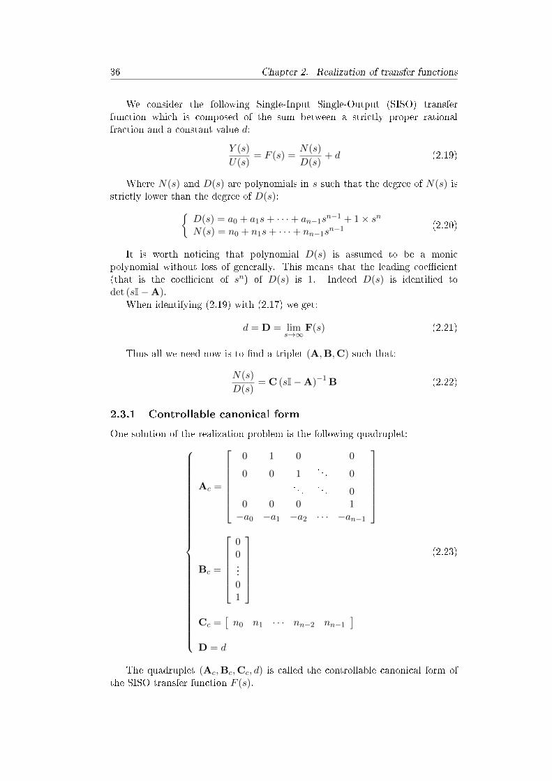
We consider the following Single-Input Single-Output (SISO) transferfunction which is composed of the sum between a strictly proper rationalfraction and a constant value d:
Y (s)
U(s)= F (s) =
N(s)
D(s)+ d (2.19)
Where N(s) and D(s) are polynomials in s such that the degree of N(s) isstrictly lower than the degree of D(s):
D(s) = a0 + a1s+ · · ·+ an−1sn−1 + 1× sn
N(s) = n0 + n1s+ · · ·+ nn−1sn−1 (2.20)
It is worth noticing that polynomial D(s) is assumed to be a monicpolynomial without loss of generally. This means that the leading coecient(that is the coecient of sn) of D(s) is 1. Indeed D(s) is identied todet (sI−A).
When identifying (2.19) with (2.17) we get:
d = D = lims→∞
F(s) (2.21)
Thus all we need now is to nd a triplet (A,B,C) such that:
N(s)
D(s)= C (sI−A)−1 B (2.22)
2.3.1 Controllable canonical form
One solution of the realization problem is the following quadruplet:
Ac =
0 1 0 0
0 0 1. . . 0
. . .. . . 0
0 0 0 1−a0 −a1 −a2 · · · −an−1
Bc =
00...01
Cc =
[n0 n1 · · · nn−2 nn−1
]D = d
(2.23)
The quadruplet (Ac,Bc,Cc, d) is called the controllable canonical form ofthe SISO transfer function F (s).

2.3. Realization of SISO transfer function 37
Alternatively the following realization is also called the controllablecanonical form of the SISO transfer function F (s). Compared with (2.23)value 1 appears in the lower diagonal of the state matrix which is obtained bychoosing a similarity transformation with value 1 on the antidiagonal (orcounter diagonal):
Aca =
0 0 0 −a0
1 0 0. . . −a1
0. . .
. . .. . . −a2
. . . 0...
0 · · · 0 1 −an−1
Bca =
10...00
Cca =
[nn−1 nn−2 · · · n1 n0
]D = d
(2.24)
To get the realization (2.23) we start by expressing the output Y (s) of SISOsystem (2.19) as follows:
Y (s) = N(s)U(s)
D(s)+ dU(s) (2.25)
Now let's focus on the following intermediate variable Z(s) which is denedas follows:
Z(s) =U(s)
D(s)=
U(s)
a0 + a1s+ a2s2 + · · ·+ an−1sn−1 + sn(2.26)
That is:
a0Z(s) + a1sZ(s) + a2s2Z(s) + · · ·+ an−1s
n−1Z(s) + snZ(s) = U(s) (2.27)
Then we dene the components of the state vector x(t) as follows:
x1(t) := z(t)x2(t) := x1(t) = z(t)x3(t) := x2(t) = z(t)...
xn(t) := xn−1(t) = z(n−1)(t)
(2.28)
Coming back in the time domain Equation (2.27) is rewritten as follows:
a0x1(t) + a1x2(t) + a2x3(t) + · · ·+ an−1xn(t) + xn(t) = u(t)⇔ xn(t) = −a0x1(t)− a1x2(t)− a2x3(t)− · · · − an−1xn(t) + u(t)
(2.29)

38 Chapter 2. Realization of transfer functions
The intermediate variable Z(s) allows us to express the output Y (s) asfollows:
Y (s) = N(s)Z(s) + dU(s) =(n0 + · · ·+ nn−1s
n−1)Z(s) + dU(s) (2.30)
That is, coming back if the time domain:
y(t) = n0z(t) + · · ·+ nn−1z(n−1)(t) + du(t) (2.31)
The use of the components of the state vector which have been previouslydened leads to the following expression of the output y(t):
y(t) = n0x1(t) + · · ·+ nn−1xn(t) + du(t) (2.32)
By combining in vector form Equations (2.28), (2.29) and (2.32) we retrievethe state-space representation (2.23).
Thus by ordering the numerator and the denominator of the transfer functionF (s) according to the increasing power of s and taking care that the leadingcoecient of the polynomial in the denominator is 1, the controllable canonicalform (2.23) of a SISO transfer function F (s) is immediate.
Example 2.1. Let's consider the following transfer function:
F (s) =(s+ 1)(s+ 2)
2(s+ 3)(s+ 4)=
s2 + 3s+ 2
2s2 + 14s+ 24(2.33)
We are looking for the controllable canonical form of this transfer function.
First we have to set to 1 the leading coecient of the polynomial whichappears in the denominator of the transfer function F (s). We get:
F (s) =0.5s2 + 1.5s+ 1
1× s2 + 7s+ 12(2.34)
Then we decompose F (s) as a sum between a strictly proper rational fractionand a constant coecient d. Constant coecient d is obtained thanks to thefollowing relationship:
d = lims→∞
F (s) = lims→∞
0.5s2 + 1.5s+ 1
1× s2 + 7s+ 12= 0.5 (2.35)
Thus the strictly proper transfer function N(s)/D(s) is obtained bysubtracting d to F (s):
N(s)
D(s)= F (s)− d =
0.5s2 + 1.5s+ 1
1× s2 + 7s+ 12− 0.5 =
−2s− 5
s2 + 7s+ 12(2.36)
We nally get:
F (s) =N(s)
D(s)+ d =
−2s− 5
s2 + 7s+ 12+ 0.5 (2.37)

2.3. Realization of SISO transfer function 39
Then we apply Equation (2.23) to get the controllable canonical form of F (s):
Ac =
[0 1−a0 −a1
]=
[0 1−12 −7
]
Bc =
[01
]Cc =
[n0 n1
]=[−5 −2
]D = 0.5
(2.38)
2.3.2 Poles and zeros of the transfer function
It is worth noticing that the numerator of the transfer function only depends onmatrices B and C whereas the denominator of the transfer function is built fromthe characteristic polynomial coming from the eigenvalues of the state matrixA.
As far as the transfer function does not depend on the state space realizationwhich is used, we can get this result by using the controllable canonical form.Indeed we can check that transfer function Cc (sI−Ac)
−1 Bc has a denominatorwhich only depends on the state matrix Ac whereas its numerator only dependson Cc, which provides the coecients of the numerator:
(sI−Ac)−1 Bc =
1
det (sI−Ac)
∗ ∗ 1∗ ∗ s...
......
∗ ∗ sn−1
0...01
⇒ Cc (sI−Ac)−1 Bc =
Cc
det (sI−Ac)
1s...
sn−1
(2.39)
More generally, the characteristic polynomial of the state matrix A setsthe denominator of the transfer function whereas the product B C sets thecoecients of the numerator of a strictly proper transfer function (that is atransfer function where D = 0). Consequently state matrix A sets the poles ofa transfer function whereas product B C sets its zeros.
2.3.3 Similarity transformation to controllable canonical form
We consider the following general state-space representation:x(t) = Ax(t) + Bu(t)y(t) = Cx(t) + Du(t)
(2.40)
where the size of the state vector x(t) is n.

40 Chapter 2. Realization of transfer functions
Use of the controllability matrix
The controllable canonical form (2.23) exists if and only if the following matrixQc, which is called the controllability matrix, has full rank:
Qc =[
B AB · · · An−1B]
(2.41)
As soon as the characteristic polynomial of matrix A is computed the statematrix Ac as well as the control matrix Bc corresponding to the controllablecanonical form are known. Thus the controllability matrix in the controllablecanonical basis, which will be denoted Qcc, can be computed as follows:
Qcc =[
Bc AcBc · · · An−1c Bc
](2.42)
At that point matrices Ac and Bc are known. The only matrix which needto be computed is the output matrix Cc. Let Pc be the change of basis matrixwhich denes the new state vector in the controllable canonical basis. From(2.8) we get:
Cc = CPc (2.43)
And: Ac = P−1
c APc
Bc = P−1c B
(2.44)
Using these two last equations within (2.42) and the fact that(P−1c APc
)k=
P−1c APc · · ·P−1
c APc︸ ︷︷ ︸k-times
= P−1c AkPc, we get the following expression of matrix
Qcc:
Qcc =[
Bc AcBc · · · An−1c Bc
]=[
P−1c B P−1
c APcP−1c B · · ·
(P−1c APc
)n−1P−1c B
]=[
P−1c B P−1
c AB · · · P−1c An−1B
]= P−1
c
[B AB · · · An−1B
]= P−1
c Qc
(2.45)
We nally get:P−1c = QccQ
−1c ⇔ Pc = QcQ
−1cc (2.46)
Furthermore the controllable canonical form (2.23) is obtained by thefollowing similarity transformation:
x(t) = Pcxc(t)⇔ xc(t) = P−1c x(t) (2.47)
Alternatively the constant nonsingular matrix P−1c can be obtained through
the state matrix A and the last row qTcof the inverse of the controllability
matrix Qc as follows:
Q−1c =
∗...∗qTc
⇒ P−1c =
qTc
qTcA...
qTcAn−1
(2.48)

2.3. Realization of SISO transfer function 41
To get this result we write from (2.8) the following similarity transformation:
Ac = P−1c APc ⇔ AcP
−1c = P−1
c A (2.49)
Let's denote det (sI−A) as follows:
det (sI−A) = sn + an−1sn−1 + · · ·+ a1s+ a0 (2.50)
Thus the coecients ai of the state matrix Ac corresponding to thecontrollable canonical form are known and matrix Ac is written as follows:
Ac =
0 1 0 0
0 0 1. . . 0
. . .. . . 0
0 0 0 1−a0 −a1 −a2 · · · −an−1
(2.51)
Furthermore let's write the unknown matrix P−1c as follows:
P−1c =
rT1...rTn
(2.52)
Thus the rows of the unknown matrix P−1c can be obtained thanks to the
following similarity transformation:
AcP−1c = P−1
c A
⇔
0 1 0 0
0 0 1. . . 0
. . .. . . 0
0 0 0 1−a0 −a1 −a2 · · · −an−1
rT1
...rTn
=
rT1...rTn
A(2.53)
Working out with the rst n− 1th rows gives the following equations:rT2 = rT1 ArT3 = rT2 A = rT1 A2
...rTn = rTn−1A = rT1 An−1
(2.54)
Furthermore from (2.8) we get the relationship Bc = P−1c B which is
rewritten as follows:
P−1c B = Bc ⇔
rT1...rTn
B =
00...01
⇔
rT1 B = 0...rTn−1B = 0rTnB = 1
(2.55)

42 Chapter 2. Realization of transfer functions
Combining (2.54) and (2.55) we get:
rT1 B = 0rT2 B = rT1 AB = 0...rTn−1B = rT1 An−2B = 0rTnB = rT1 An−1B = 1
(2.56)
These equations can in turn be written in matrix form as:
rT1[
B AB · · · An−2B An−1B]
=[
0 0 · · · 0 1]
(2.57)
Let's introduce the controllability matrix Qc:
Qc =[
B AB · · · An−1B]
(2.58)
Assuming that matrix Qc has full rank we get:
rT1 Qc =[
0 0 · · · 0 1]⇔ rT1 =
[0 0 · · · 0 1
]Q−1c (2.59)
From the preceding equation it is clear that rT1 is the last row of the inverseof the controllability matrix Qc. We will denote it qT
c:
rT1 := qTc
(2.60)
Having the expression of rT1 we can then go back to (2.54) and construct allthe rows of P−1
c .
Example 2.2. We consider the following general state-space representation:x(t) = Ax(t) + Bu(t)y(t) = Cx(t) + Du(t)
(2.61)
where:
A =
[28.5 −17.558.5 −35.5
]
B =
[24
]C =
[7 −4
]D = 0.5
(2.62)
We are looking for the controllable canonical form of this state-spacerepresentation.
First we build the controllability matrix Qc from (2.41):
Qc =[
B AB]
=
[2 −134 −25
](2.63)
2.3. Realization of SISO transfer function 43
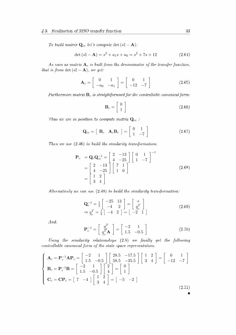
To build matrix Qcc let's compute det (sI−A):
det (sI−A) = s2 + a1s+ a0 = s2 + 7s+ 12 (2.64)
As soon as matrix Ac is built from the denominator of the transfer function,that is from det (sI−A), we get:
Ac =
[0 1−a0 −a1
]=
[0 1−12 −7
](2.65)
Furthermore matrix Bc is straightforward for the controllable canonical form:
Bc =
[01
](2.66)
Thus we are in position to compute matrix Qcc :
Qcc =[
Bc AcBc
]=
[0 11 −7
](2.67)
Then we use (2.46) to build the similarity transformation:
Pc = QcQ−1cc =
[2 −134 −25
] [0 11 −7
]−1
=
[2 −134 −25
] [7 11 0
]=
[1 23 4
] (2.68)
Alternatively we can use (2.48) to build the similarity transformation:
Q−1c = 1
2
[−25 13−4 2
]=
[∗qTc
]⇒ qT
c= 1
2
[−4 2
]=[−2 1
] (2.69)
And:
P−1c =
[qTc
qTcA
]=
[−2 11.5 −0.5
](2.70)
Using the similarity relationships (2.8) we nally get the followingcontrollable canonical form of the state-space representation:
Ac = P−1c APc =
[−2 11.5 −0.5
] [28.5 −17.558.5 −35.5
] [1 23 4
]=
[0 1−12 −7
]Bc = P−1
c B =
[−2 11.5 −0.5
] [24
]=
[01
]Cc = CPc =
[7 −4
] [ 1 23 4
]=[−5 −2
](2.71)

44 Chapter 2. Realization of transfer functions
Iterative method
Equivalently change of basis matrix Pc of the similarity transformation can beobtained as follows:
Pc =[c1 c2 · · · cn
](2.72)
where: det (sI−A) = sn + an−1s
n−1 + · · ·+ a1s+ a0
cn = Bck = Ack+1 + akB ∀ n− 1 ≥ k ≥ 1
(2.73)
To get this result we write from (2.8) the following similarity transformation:
Ac = P−1c APc ⇔ PcAc = APc (2.74)
Let's denote det (sI−A) as follows:
det (sI−A) = sn + an−1sn−1 + · · ·+ a1s+ a0 (2.75)
Thus the coecients ai of the state matrix Ac corresponding to thecontrollable canonical form are known and matrix Ac written as follows:
Ac =
0 1 0 0
0 0 1. . . 0
. . .. . . 0
0 0 0 1−a0 −a1 −a2 · · · −an−1
(2.76)
Furthermore let's write the unknown change of basis matrix Pc as follows:
Pc =[c1 c2 · · · cn
](2.77)
Thus the columns of the unknown matrix Pc can be obtained thanks to thesimilarity transformation:
PcAc = APc
⇔[c1 c2 · · · cn
]
0 1 0 0
0 0 1. . . 0
. . .. . . 0
0 0 0 1−a0 −a1 −a2 · · · −an−1
= A[c1 c2 · · · cn
]
(2.78)
That is:0 = a0cn + Ac1
c1 = a1cn + Ac2...cn−1 = an−1cn + Acn
⇔
0 = a0cn + Ac1
ck = Ack+1 + akcn ∀ n− 1 ≥ k ≥ 1(2.79)

2.3. Realization of SISO transfer function 45
Furthermore from (2.8) we get the relationship Bc = P−1c B which is
rewritten as follows:
PcBc = B⇔[c1 c2 · · · cn
]
00...01
= B⇒ cn = B (2.80)
Combining the last equation of (2.79) with (2.80) gives the proposed result:cn = Bck = Ack+1 + akB ∀ n− 1 ≥ k ≥ 1
(2.81)
Example 2.3. We consider the following general state-space representation:x(t) = Ax(t) + Bu(t)y(t) = Cx(t) + Du(t)
(2.82)
where:
A =
[28.5 −17.558.5 −35.5
]
B =
[24
]C =
[7 −4
]D = 0.5
(2.83)
This is the same state-space representation than the one which has been usedin the previous example. We have seen that the similarity transformation whichleads to the controllable canonical form is the following:
P−1c =
[−2 11.5 −0.5
](2.84)
It is easy to compute matrix Pc, that is the inverse of P−1c . We get the
following expression:
Pc =
[1 23 4
](2.85)
We will check the expression of matrix Pc thanks to the iterative methodproposed in (2.73). We get:
det (sI−A) = s2 + 7s+ 12
c2 = B =
[24
]c1 = Ac2 + a1B =
[28.5 −17.558.5 −35.5
] [24
]+ 7
[24
]=
[13
] (2.86)

46 Chapter 2. Realization of transfer functions
Thus we fortunately retrieve the expression of matrix Pc:
Pc =[c1 c2
]=
[1 23 4
](2.87)
2.3.4 Observable canonical form
Another solution of the realization problem is the following quadruplet:
Ao =
0 0 0 −a0
1 0 0. . . −a1
0 1 0. . . −a2
.... . .
. . ....
0 0 1 −an−1
Bo =
n0
n1...
nn−2
nn−1
Co =
[0 0 · · · 0 1
]D = d
(2.88)
The quadruplet (Ao,Bo,Co, d) is called the observable canonical form of theSISO transfer function F (s).
Alternatively the following realization is also called the observablecanonical form of the SISO transfer function F (s). Compared with (2.88)value 1 appears in the upper diagonal of the state matrix which is obtained bychoosing a similarity transformation with value 1 on the antidiagonal (or

2.3. Realization of SISO transfer function 47
counter diagonal):
Aoa =
0 1 0 0
0 0 1. . . 0
. . .. . . 0
0 0 0 1−a0 −a1 −a2 · · · −an−1
Boa =
nn−1
nn−2
· · ·n1
n0
Coa =
[1 0 · · · 0 0
]D = d
(2.89)
To get the realization (2.88) we start by expressing the output Y (s) of SISOsystem (2.19) as follows:
Y (s)
U(s)=N(s)
D(s)+ d⇔ (Y (s)− dU(s))D(s) = N(s)U(s) (2.90)
That is:(a0 + a1s+ a2s
2 + · · ·+ an−1sn−1 + sn
)(Y (s)− dU(s))
=(n0 + n1s+ · · ·+ nn−1s
n−1)U(s) (2.91)
Dividing by sn we get:(a0
sn+
a1
sn−1+
a2
sn−2+ · · ·+ an−1
s+ 1)
(Y (s)− dU(s))
=(n0
sn+
n1
sn−1+
n2
sn−2+ · · ·+ nn−1
s
)U(s) (2.92)
When regrouping the terms according the increasing power of 1s we obtain:
Y (s) = dU(s) +1
s(αn−1U(s)− an−1Y (s)) +
1
s2(αn−2U(s)− an−2Y (s)) +
· · ·+ 1
sn(α0U(s)− a0Y (s)) (2.93)
Where:αi = ni + d ai (2.94)
That is:
Y (s) = dU(s) +1
s
(αn−1U(s)− an−1Y (s) +
1
s
(αn−2U(s)− an−2Y (s)
)+
1
s
(· · ·+ 1
s
(α0U(s)− a0Y (s)
))))(2.95)

48 Chapter 2. Realization of transfer functions
Then we dene the Laplace transform of the components of the state vectorx(t) as follows:
sX1(s) = α0U(s)− a0Y (s)sX2(s) = α1U(s)− a1Y (s) +X1(s)sX3(s) = α2U(s)− a2Y (s) +X2(s)...sXn(s) = αn−1U(s)− an−1Y (s) +Xn−1(s)
(2.96)
So we get:
Y (s) = dU(s) +1
s
(sXn(s)
)= dU(s) +Xn(s) (2.97)
Replacing Y (s) by Xn(s) and using the fact that αi = ni + d ai Equation(2.96) is rewritten as follows:
sX1(s) = α0U(s)− a0 (dU(s) +Xn(s))= −a0Xn(s) + n0U(s)
sX2(s) = α1U(s)− a1 (dU(s) +Xn(s)) +X1(s)= X1(s)− a1Xn(s) + n1U(s)
sX3(s) = α2U(s)− a2 (dU(s) +Xn(s)) +X2(s)= X2(s)− a2Xn(s) + n2U(s)
...sXn(s) = αn−1U(s)− an−1 (dU(s) +Xn(s)) +Xn−1(s)
= Xn−1(s)− an−1Xn(s) + nn−1U(s)
(2.98)
Coming back in the time domain we nally get:
x1(t) = −a0xn(t) + n0u(t)x2(t) = x1(t)− a1xn(t) + n1u(t)x3(t) = x2(t)− a2xn(t) + n2u(t)...xn(t) = xn−1(t)− an−1xn(t) + nn−1u(t)
(2.99)
And:
y(t) = xn(t) + d u(t) (2.100)
The preceding equations written in vector form leads to the observablecanonical form of Equation (2.88).
Thus by ordering the numerator and the denominator of the transfer functionF (s) according to the increasing power of s and taking care that the leadingcoecient of the polynomial in the denominator is 1, the observable canonicalform (2.88) of a SISO transfer function F (s) is immediate.
Example 2.4. Let's consider the following transfer function:
F (s) =(s+ 1)(s+ 2)
2(s+ 3)(s+ 4)=
s2 + 3s+ 2
2s2 + 14s+ 24(2.101)

2.3. Realization of SISO transfer function 49
We are looking for the observable canonical form of this transfer function.
As in the preceding example we rst set to 1 the leading coecient of thepolynomial which appears in the denominator of the transfer function F (s). Weget:
F (s) =0.5s2 + 1.5s+ 1
1× s2 + 7s+ 12(2.102)
Then we decompose F (s) as a sum between a strictly proper rational fractionand a constant coecient d. Constant coecient d is obtained thanks to thefollowing relationship:
d = lims→∞
F(s) = lims→∞
0.5s2 + 1.5s+ 1
1× s2 + 7s+ 12= 0.5 (2.103)
Thus the strictly proper transfer function N(s)/D(s) is obtained bysubtracting d to F (s):
N(s)
D(s)= F (s)− d =
0.5s2 + 1.5s+ 1
1× s2 + 7s+ 12− 0.5 =
−2s− 5
s2 + 7s+ 12(2.104)
We nally get:
F (s) =N(s)
D(s)+ d =
−2s− 5
s2 + 7s+ 12+ 0.5 (2.105)
Then we apply Equation (2.88) to get the observable canonical form of F (s):
Ao =
[0 −a0
1 −a1
]=
[0 −121 −7
]
Bo =
[n0
n1
]=
[−5−2
]Co =
[0 1
]D = 0.5
(2.106)
2.3.5 Similarity transformation to observable canonical form
We consider the following general state-space representation:x(t) = Ax(t) + Bu(t)y(t) = Cx(t) + Du(t)
(2.107)
where the size of the state vector x(t) is n.

50 Chapter 2. Realization of transfer functions
Use of the observability matrix
The observable canonical form (2.88) exists if and only if the following matrixQo, which is called the observability matrix, has full rank:
Qo =
C
CA...
CAn−1
(2.108)
As soon as the characteristic polynomial of matrix A is computed the statematrix Ao as well as the output matrix Co corresponding to the observablecanonical form are known. Thus the observability matrix in the observablecanonical basis, which will be denoted Qoo, can be computed as follows:
Qoo =
Co
CoAo...
CoAn−1o
(2.109)
At that point matrices Ao and Co are known. The only matrix which needto be computed is the control matrix Bo. Let Po be the change of basis matrixwhich denes the new state vector in the observable canonical basis. From (2.8)we get:
Bo = P−1o B (2.110)
And: Ao = P−1
o APo
Co = CPo(2.111)
Using these last two equations within (2.109) leads to the followingexpression of matrix Qoo:
Qoo =
Co
CoAo...
CoAn−1o
=
CPo
CPoP−1o APo...
CPo
(P−1o APo
)n−1
=
CPo
CAPo...
CAn−1Po
=
C
CA...
CAn−1
Po
= QoPo
(2.112)
We nally get:Po = Q−1
o Qoo ⇔ P−1o = Q−1
oo Qo (2.113)
Furthermore the observable canonical form (2.88) is obtained by thefollowing similarity transformation:
x(t) = Poxo(t)⇔ xo(t) = P−1o x(t) (2.114)

2.3. Realization of SISO transfer function 51
Alternatively the constant nonsingular matrix Po can be obtained throughthe state matrix A and the last column q
oof the inverse of the observability
matrix Qo as follows:
Q−1o =
[∗ · · · ∗ q
o
]⇒ Po =
[qo
Aqo· · · An−1q
o
](2.115)
To get this result we write from (2.8) the following similarity transformation:
Ao = P−1o APo ⇔ PoAo = APo (2.116)
Let's denote det (sI−A) as follows:
det (sI−A) = sn + an−1sn−1 + · · ·+ a1s+ a0 (2.117)
Thus the coecients ai of the state matrix Ao corresponding to theobservable canonical form are known and matrix Ao is written as follows:
Ao =
0 0 0 −a0
1 0 0. . . −a1
0 1 0. . . −a2
.... . .
. . ....
0 0 1 −an−1
(2.118)
Furthermore let's write the unknown matrix Po as follows:
Po =[c1 · · · cn
](2.119)
Thus the columns of the unknown change of basis matrix Po can be obtainedthanks to the following similarity transformation:
PoAo = APo
⇔[c1 · · · cn
]
0 0 0 −a0
1 0 0. . . −a1
0 1 0. . . −a2
.... . .
. . ....
0 0 1 −an−1
= A
[c1 · · · cn
]
(2.120)
Working out with the rst n− 1th columns gives the following equations:c2 = Ac1
c3 = Ac2 = A2c1...cn = Acn−1 = An−1c1
(2.121)
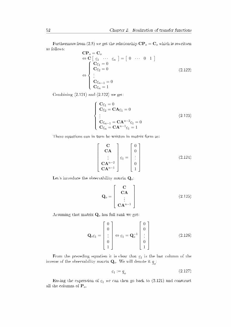
52 Chapter 2. Realization of transfer functions
Furthermore from (2.8) we get the relationship CPo = Co which is rewrittenas follows:
CPo = Co
⇔ C[c1 · · · cn
]=[
0 · · · 0 1]
⇔
Cc1 = 0Cc2 = 0...Ccn−1 = 0Ccn = 1
(2.122)
Combining (2.121) and (2.122) we get:
Cc1 = 0Cc2 = CAc1 = 0...Ccn−1 = CAn−2c1 = 0Ccn = CAn−1c1 = 1
(2.123)
These equations can in turn be written in matrix form as:C
CA...
CAn−2
CAn−1
c1 =
00...01
(2.124)
Let's introduce the observability matrix Qo:
Qo =
C
CA...
CAn−1
(2.125)
Assuming that matrix Qo has full rank we get:
Qoc1 =
00...01
⇔ c1 = Q−1o
00...01
(2.126)
From the preceding equation it is clear that c1 is the last column of theinverse of the observability matrix Qo. We will denote it q
o:
c1 := qo
(2.127)
Having the expression of c1 we can then go back to (2.121) and constructall the columns of Po.

2.3. Realization of SISO transfer function 53
Example 2.5. We consider the following general state-space representation:x(t) = Ax(t) + Bu(t)y(t) = Cx(t) + Du(t)
(2.128)
where:
A =
[28.5 −17.558.5 −35.5
]
B =
[24
]C =
[7 −4
]D = 0.5
(2.129)
We are looking for the observable canonical form of this state-spacerepresentation.
First we build the observability matrix Qo from (2.108):
Qo =
[C
CA
]=
[7 −4
−34.5 19.5
](2.130)
To build matrix Qoo let's compute det (sI−A):
det (sI−A) = s2 + a1s+ a0 = s2 + 7s+ 12 (2.131)
As soon as matrix Ao is built from the denominator of the transfer function,that is from det (sI−A), we get:
Ao =
[0 −a0
1 −a1
]=
[0 −121 −7
](2.132)
Furthermore matrix Co is straightforward for the observable canonical form:
Co =[
0 1]
(2.133)
Thus we are in position to compute matrix Qoo :
Qoo =
[Co
CoAo
]=
[0 11 −7
](2.134)
Then we use (2.113) to build the similarity transformation:
Po = Q−1o Qoo =
[7 −4
−34.5 19.5
]−1 [0 11 −7
]= 1−1.5
[19.5 434.5 7
] [0 11 −7
]= 2
3
[−19.5 −4−34.5 −7
] [0 11 −7
]= 2
3
[−4 8.5−7 14.5
](2.135)

54 Chapter 2. Realization of transfer functions
Alternatively we can use (2.115) to build the similarity transformation:
Q−1o = 2
3
[−19.5 −4−34.5 −7
]=[∗ q
o
]⇒ q
o= 2
3
[−4−7
] (2.136)
And:
Po =[qo
Aqo
]=
2
3
[−4 8.5−7 14.5
](2.137)
Using the similarity relationships (2.8) we nally get the following observablecanonical form of the state-space representation:
Ao = P−1o APo =
[14.5 −8.5
7 −4
] [28.5 −17.558.5 −35.5
]23
[−4 8.5−7 14.5
]=
[0 −121 −7
]Bo = P−1
o B =
[14.5 −8.5
7 −4
] [24
]=
[−5−2
]Co = CPo =
[7 −4
]23
[−4 8.5−7 14.5
]=[
0 1]
(2.138)
Iterative method
Equivalently the inverse of the change of basis matrix Po of the similaritytransformation can be obtained as follows:
P−1o =
rT1rT2...rTn
(2.139)
where: det (sI−A) = sn + an−1s
n−1 + · · ·+ a1s+ a0
rTn = CrTk = rTk+1A + akC ∀ n− 1 ≥ k ≥ 1
(2.140)
To get this result we write from (2.8) the following similarity transformation:
Ao = P−1o APo ⇔ AoP
−1o = P−1
o A (2.141)
Let's denote det (sI−A) as follows:
det (sI−A) = sn + an−1sn−1 + · · ·+ a1s+ a0 (2.142)
Thus the coecients ai of the state matrix Ao corresponding to theobservable canonical form are known and matrix Ao is written as follows:
Ao =
0 0 0 −a0
1 0 0. . . −a1
0 1 0. . . −a2
.... . .
. . ....
0 0 1 −an−1
(2.143)

2.3. Realization of SISO transfer function 55
Furthermore let's write the inverse of the unknown change of basis matrixPo as follows:
P−1o =
rT1rT2...rTn
(2.144)
Thus the columns of the unknown matrix Po can be obtained thanks to thesimilarity transformation:
AoP−1o = P−1
o A
⇔
0 0 0 −a0
1 0 0. . . −a1
0 1 0. . . −a2
.... . .
. . ....
0 0 1 −an−1
rT1rT2...rTn
=
rT1rT2...rTn
A(2.145)
That is:−a0r
Tn = rT1 A
rT1 − a1rTn = rT2 A
...rTn−1 − an−1r
Tn = rTnA
⇔
0 = rT1 A + a0rTn
rTk = rTk+1A + akrTn ∀ n− 1 ≥ k ≥ 1
(2.146)
Furthermore from (2.8) we get the relationship Co = CPo which is rewrittenas follows:
CoP−1o = C⇔
[0 · · · 0 1
]rT1rT2...rTn
= C⇒ rTn = C (2.147)
Combining the last equation of (2.146) with (2.147) gives the proposedresult:
rTn = CrTk = rTk+1A + akC ∀ n− 1 ≥ k ≥ 1
(2.148)
Example 2.6. We consider the following general state-space representation:
x(t) = Ax(t) + Bu(t)y(t) = Cx(t) + Du(t)
(2.149)

56 Chapter 2. Realization of transfer functions
where:
A =
[28.5 −17.558.5 −35.5
]
B =
[24
]C =
[7 −4
]D = 0.5
(2.150)
This is the same state-space representation than the one which has been usedin the previous example. We have seen that the similarity transformation whichleads to the controllable canonical form is the following:
Po =2
3
[−4 8.5−7 14.5
](2.151)
It is easy to compute matrix P−1o , that is the inverse of Po. We get the
following expression:
P−1o =
[14.5 −8.5
7 −4
](2.152)
We will check the expression of matrix P−1o thanks to the iterative method
proposed in (2.140). We get:
det (sI−A) = s2 + 7s+ 12rT2 = C =
[7 −4
]rT1 = rT2 A + a1C =
[7 −4
] [ 28.5 −17.558.5 −35.5
]+ 7
[7 −4
]=[
14.5 −8.5]
(2.153)
Thus we fortunately retrieve the expression of matrix P−1o :
P−1o =
[rT1rT2
]=
[14.5 −8.5
7 −4
](2.154)
2.3.6 Diagonal (or modal) form
One particular useful canonical form is called the diagonal (Jordan) or modalform. The diagonal form is obtained thanks to the partial fraction expansion oftransfer function F (s). This is a diagonal representation of the state-space modelwhen all the poles of F (s) are distinct; otherwise this is a Jordan representation.

2.3. Realization of SISO transfer function 57
Transfer function with distinct poles
Assume for now that transfer function F (s) has distinct poles λi. Then thepartial fraction expansion of F (s) reads:
Y (s)U(s) = F (s) = N(s)
D(s) + d
= N(s)(s−λ1)(s−λ2)···(s−λn) + d
= r1s−λ1 + r2
s−λ2 + · · ·+ rns−λn + d
(2.155)
Number ri is called the residue of transfer function F (s) in λi. When themultiplicity of the pole (or eigenvalue) λi is 1 it is clear from the precedingrelationship that the residue ri can be obtained thanks to the following formula:
ri = (s− λi)F (s)|s=λi (2.156)
Now we dene constants bi and ci such that the product bici is equal to ri:
ri = ci bi (2.157)
Consequently transfer function F (s) can be written as follows:
F (s) =c1 b1s− λ1
+c2 b2s− λ2
+ · · ·+ cn bns− λn
+ d (2.158)
Then we dene the Laplace transform of the componentsx1(t), x2(t), · · · , xn(t) of the state vector x(t) as follows:
X1(s)U(s) = b1
s−λ1X2(s)U(s) = b2
s−λ2...Xn(s)U(s) = bn
s−λn
(2.159)
Using (2.159) transfer function F (s) can be written as follows:
Y (s)U(s) = F (s) = c1
X1(s)U(s) + c2
X2(s)U(s) + · · ·+ cn
Xn(s)U(s) + d
⇒ Y (s) = c1X1(s) + c2X2(s) + · · ·+ cnXn(s) + dU(s)(2.160)
Coming back to the time domain we get:
y(t) = c1x1(t) + c2x2(t) + · · ·+ cnxn(t) + du(t) (2.161)
Whereas in the time domain (2.159) reads:x1(t) = λ1x1(t) + b1u(t)x2(t) = λ2x2(t) + b2u(t)...xn(t) = λnxn(t) + bnu(t)
(2.162)
Equations (2.162) and (2.161) lead to the following state-spacerepresentation, which is called the diagonal (Jordan) or modal form:

58 Chapter 2. Realization of transfer functions
x(t) = Ax(t) + Bu(t)y(t) = Cx(t) + Du(t)
(2.163)
where:
A =
λ1 0 0
0 λ2...
.... . . 0
0 · · · 0 λn
B =
b1b2...bn
C =
[c1 c2 · · · cn
]D = d
(2.164)
Example 2.7. Let's consider the following transfer function:
F (s) =(s+ 1)(s+ 2)
2(s+ 3)(s+ 4)=
s2 + 3s+ 2
2s2 + 14s+ 24(2.165)
We are looking for the diagonal form of this transfer function.
First we have to set to 1 the leading coecient of the polynomial whichappears in the denominator of the transfer function F (s). We get:
F (s) =0.5s2 + 1.5s+ 1
1× s2 + 7s+ 12(2.166)
Then we decompose F (s) as a sum between a strictly proper rational fractionand a constant coecient d. Constant coecient d is obtained thanks to thefollowing relationship:
d = lims→∞
F(s) = lims→∞
0.5s2 + 1.5s+ 1
1× s2 + 7s+ 12= 0.5 (2.167)
Thus the strictly proper transfer function N(s)/D(s) is obtained bysubtracting d to F (s):
N(s)
D(s)= F (s)− d =
0.5s2 + 1.5s+ 1
1× s2 + 7s+ 12− 0.5 =
−2s− 5
s2 + 7s+ 12(2.168)
The two poles of F (s) are −3 and −4. Thus the partial fraction expansionof F (s) reads:
F (s) =r1
s+ 3+
r2
s+ 4+ d =
r1
s+ 3+
r2
s+ 4− 0.5 (2.169)

2.3. Realization of SISO transfer function 59
where the residues r1 and r2 are: r1 = (s+ 3)F (s)|s=−3(s+1)(s+2)
2(s+4)
∣∣∣s=−3
= (−3+1)(−3+2)2(−3+4) = 1
r2 = (s+ 4)F (s)|s=−4(s+1)(s+2)
2(s+3)
∣∣∣s=−4
= (−4+1)(−4+2)2(−4+3) = −3
(2.170)
We nally get:
F (s) =N(s)
D(s)+ d =
1
s+ 3+−3
s+ 4+ 0.5 (2.171)
Residues r1 and r2 are expressed for example as follows:r1 = 1 = 1× 1 = c1 × b1r2 = −3 = −3× 1 = c2 × b2
(2.172)
Then we apply Equation (2.164) to get the diagonal canonical form of F (s):
A =
[λ1 00 λ2
]=
[−3 00 −4
]
B =
[b1b2
]=
[1−3
]C =
[c1 c2
]=[
1 1]
D = d = 0.5
(2.173)
Similarity transformation to diagonal form
Assume that state matrix A has distinct eigenvalues λi. Starting from a
realization
(A B
C d
)let Pm be the change of basis matrix such that:
Am =
λ1 0 0
0 λ2...
.... . . 0
0 · · · 0 λn
= P−1m APm (2.174)
We will denote Pm as follows:
Pm =[v1 v2 · · · vn
](2.175)
It can be seen that vectors vi are the eigenvectors of matrix A. Indeed letλi be an eigenvalue of A. Then:
Av1 = λ1v1...
Avn = λnvn
(2.176)

60 Chapter 2. Realization of transfer functions
Writing this equation in vector form leads to the following relationship:
[v1 v2 · · · vn
]λ1 0 0
0 λ2...
.... . . 0
0 · · · 0 λn
= A[v1 v2 · · · vn
](2.177)
That is:
Pm
λ1 0 0
0 λ2...
.... . . 0
0 · · · 0 λn
= APm (2.178)
Or equivalently: λ1 0 0
0 λ2...
.... . . 0
0 · · · 0 λn
= P−1m APm (2.179)
The inverse of the change of basis matrix Pn can be written in terms of rowsas follows:
P−1m =
wT1wT2...wTn
(2.180)
It can be seen that vectors wi are the eigenvectors of matrix AT . Indeedlet λi be an eigenvalue of A, which is also an eigenvalue of AT as far asdet (sI−A) = det (sI−A)T = det
(sI−AT
). Then:
ATwi = λiwi ⇒ wTi A = λiwTi (2.181)
Thus by multiplying by vj and using the fact that vj is an eigenvector of A,that is Avj = λjvj , we get:
λiwTi vj = wTi Avj = λjw
Ti vj ⇒ (λi − λj)wTi vj = 0 (2.182)
Since λi 6= λj ∀i 6= j we nally get:
wTi vj = 0 if i 6= j (2.183)
As far as wi and vj are dened to within a constant we impose wTi vj =1 if i = j. Consequently:
wTi vj =
1 if i = j0 if i 6= j
(2.184)

2.3. Realization of SISO transfer function 61
Transfer function with complex conjugate pair of poles
If some of the poles are complex so are the residues and so is the diagonal form.This may be inconvenient. We will see hereafter how to retrieve real matricescorresponding to the diagonal form.
Assume that λ and λ is a complex conjugate pair of poles of F (s):
F (s) =r1
s− λ+
r1
s− λ(2.185)
Let α be the real part of the pole λ and β its imaginary part:
λ = α+ jβ ⇔ λ = α− jβ (2.186)
According to the preceding section the state-space representation of F (s) isthe following:
Am =
[λ 0
0 λ
]=
[α+ jβ 0
0 α− jβ
]
Bm =
[b1b1
]Cm =
[c1 c1
]D = 0
(2.187)
Where:
r1 = b1c1 ⇒ r1 = b1c1 (2.188)
It is clear that the diagonal form of transfer function F (s) is complex. Fromthe preceding realization we get the following equations:
x1(t) = (α+ jβ)x1(t) + b1u(t)
x2(t) = (α− jβ)x2(t) + b1u(t)(2.189)
We deduce from the preceding equation that the state components x1(t) andx2(t) are complex conjugate. Let xR(t) be the real part of x1(t) and xI(t) itsimaginary part:
x1(t) = xR(t) + jxI(t)⇒ x2(t) = x1(t) = xR(t)− jxI(t) (2.190)
Thus Equation (2.189) reads:xR(t) + jxI(t) = (α+ jβ) (xR(t) + jxI(t)) + b1u(t)
xR(t)− jxI(t) = (α− jβ) (xR(t)− jxI(t)) + b1u(t)(2.191)
We deduce two new equations from the two preceding equations as follows:the rst new equation is obtained by adding the two preceding equations and

62 Chapter 2. Realization of transfer functions
dividing the result by 2 whereas the second new equation is obtained bysubtracting the two preceding equations and dividing the result by 2j. We get:
xR(t) = αxR(t)− βxI(t) + b1+b12 u(t)
xI(t) = βxR(t) + αxI(t) + b1−b12j u(t)
(2.192)
As far as the output y(t) is concerned we can express it as a function of thenew components xR(t) and xI(t) of the state vector:
y(t) = c1x1(t) + c1x1(t)= c1 (xR(t) + jxI(t)) + c1 (xR(t)− jxI(t))= (c1 + c1)xR(t) + j (c1 − c1)xI(t)
(2.193)
Consequently the complex diagonal form in Equation (2.187) is rendered realby using the real part and the imaginary part of the complex state componentwhich appear in the state vector rather than the complex state component andits conjugate. Indeed Equations (2.192) and (2.193) lead to the following state-space representation where matrices (Am,Bm,Cm,D) are real:
Am =
[α −ββ α
]
Bm =
[b1+b1
2b1−b1
2j
]
Cm =[
(c1 + c1) j (c1 − c1)]
D = 0
(2.194)
It can be seen that complex matrix A has the same determinant than thereal matrix Am:
det
(sI−
[α+ jβ 0
0 α− jβ
])= det
(sI−
[α −ββ α
])(2.195)
Example 2.8. Let's consider the following transfer function:
F (s) =s+ 2
s2 − 2s+ 5(2.196)
The two poles of F (s) are λ1 = 1 + 2j and λ1 = 1 − 2j. Thus the partialfraction expansion of F (s) reads:
F (s) =s+ 2
s2 − 2s+ 5=
s+ 2
(s− λ1)(s− λ1)=
r1
s− λ1+
r2
s− λ1
where λ1 = 1 + 2j
(2.197)where the residues r1 and r2 are: r1 = (s− λ1)F (s)|s=λ1 = s+2
s−λ1
∣∣∣s=λ1
= 3+2j4j = 2−3j
4
r2 = (s− λ1)F (s)∣∣s=λ1
= s+2s−λ1
∣∣∣s=λ1
= 3−2j−4j = 2+3j
4 = r1
(2.198)

2.3. Realization of SISO transfer function 63
We nally get:
F (s) =r1
s− λ1+
r2
s− λ1
=2−3j
4
s− (1 + 2j)+
2+3j4
s− (1− 2j)(2.199)
Residues r1 and r2 are expressed for example as follows:r1 = 2−3j
4 = (2− 3j)× 14 = c1 × b1
r2 = 2+3j4 = (2 + 3j)× 1
4 = c1 × b1(2.200)
Then we apply Equation (2.164) to get the diagonal canonical form of F (s):
Am =
[λ1 0
0 λ1
]=
[α+ jβ 0
0 α− jβ
]=
[1 + 2j 0
0 1− 2j
]
Bm =
[b1b1
]= 1
4
[11
]Cm =
[c1 c1
]=[
2− 3j 2 + 3j]
D = 0
(2.201)
This complex diagonal form realization is rendered real by using (2.194):
Am =
[α −ββ α
]=
[1 −22 1
]
Bm =
[b1+b1
2b1−b1
2j
]= 1
4
[10
]
Cm =[
(c1 + c1) j (c1 − c1)]
=[
4 6]
D = 0
(2.202)
For both realizations we can check that F (s) = Cm (sI−Am)−1 Bm+D butin the last realzation matrices (Am,Bm,Cm,D) are real.
2.3.7 Algebraic and geometric multiplicity of an eigenvalue
The algebraic multiplicity ni of an eigenvalue λi of matrix A ∈ Rn×n is thenumber of times λi appears as a root of the characteristic polynomial det(sI−A).
The geometric multiplicity qi of an eigenvalue λi of matrix A ∈ Rn×n is thedimension of the kernel of λiI−A.
If for every eigenvalue of A the geometric multiplicity equals the algebraicmultiplicity, then matrix A is said to be diagonalizable

64 Chapter 2. Realization of transfer functions
Example 2.9. Let's consider the following matrix:
A =
[2 30 2
](2.203)
We have:det(sI−A) = (s− 2)2 (2.204)
Consequently the algebraic multiplicity of eigenvalue λ1 = 2 is n1 = 2.In order to get the geometric multiplicity of eigenvalue λ1 we consider the
following matrix:
λ1I−A =
[0 −30 0
](2.205)
The dimension of the kernel of λ1I − A is clearly 1. Consequently thegeometric multiplicity of eigenvalue λ1 is q1 = 1.
2.3.8 Jordan form and generalized eigenvectors
Matrix A is not diagonalizable when there is at least one eigenvalue with ageometric multiplicity (dimension of its eigenspace) which is strictly less thanits algebraic multiplicity. If for every eigenvalue of A the geometric multiplicityequals the algebraic multiplicity then A is diagonalizable. If not, the diagonalform of matrix A is replaced by its Jordan form which is achieved through theso-called generalized eigenvectors.
A nonzero vector vλi which satises the following properties is called ageneralized eigenvector of A corresponding to eigenvalue λi:
(A− λiI)k vλi = 0
(A− λiI)k−1 vλi 6= 0(2.206)
It is clear that when k = 1 the preceding denition leads to the usualdenition of eigenvector.
It can be shown that:
ker(
(A− λiI)k)⊂ ker
((A− λiI)k+1
)(2.207)
Furthermore if A is an n × n matrix with an eigenvalue λi with algebraicmultiplicity ni then there is some integer νi ≤ ni such that the following propertyholds:
dim (ker ((A− λiI)νi)) = ni (2.208)
The Jordan block Jλi of matrix A corresponding of eigenvalue λi withalgebraic multiplicity ni is the following ni × ni matrix:
Jλi =
λi 1 0 · · · 00 λi 1 0 · · ·...
. . .. . .
. . .
λi 10 · · · · · · 0 λi
︸ ︷︷ ︸
ni terms
(2.209)

2.3. Realization of SISO transfer function 65
To get the Jordan form of any n × n square matrix A with eigenvalues λiwith algebraic multiplicity ni we must compute the nullspace of (A− λiI)ni orequivalently the nullspace of (A− λiI)n (in that situation there is no need toknow ni). Let vλi,ni be a vector which spans the nullspace of (A− λiI)ni butwhich does not belong to the nullspace of (A− λiI)ni−1:
(A− λiI)ni vλi,ni = 0
(A− λiI)ni−1 vλi,ni 6= 0(2.210)
Then the following chain of vectors can be formed:vλi,ni−1 = (A− λiI) vλi,nivλi,ni−2 = (A− λiI) vλi,ni−1 = (A− λiI)2 vλi,ni...
vλi,1 = (A− λiI)ni−1 vλi,ni
(2.211)
Let Pλi be the matrix formed by the chain of vectors[vλi,1 · · · vλi,ni
].
Then the Jordan form J of matrix A of order n corresponding is obtained as:
J = P−1AP where
P =
[Pλ1 · · · Pλn
]Pλi =
[vλi,1 · · · vλi,ni
] (2.212)
Transfer function with multiple poles on the same location
Now assume that transfer function F (s) has a pole λ of multiplicity n. Partialfraction expansion of F (s) results in:
Y (s)
U(s)= F (s) =
r1
s− λ+
r2
(s− λ)2+ · · ·+ rn
(s− λ)n+ d (2.213)
It is clear from the preceding relationship that the numbers ri ∀ n ≥ i ≥ 1can be obtained thanks to the following formula:
ri =1
(n− i)!dn−i
dsn−i((s− λ)nF (s))
∣∣∣∣s=λ
∀ n ≥ i ≥ 1 (2.214)
Number r1 is called the residue of transfer function F (s) in λ.Then we dene the Laplace transform of the components x1(t), · · · , xn(t) of
the state vector x(t) as follows:
Xi(s)
U(s)=
1
(s− λ)n−i+1∀ n ≥ i ≥ 1 (2.215)
Using (2.215) transfer function F (s) can be written as follows:
Y (s)U(s) = F (s) = r1
Xn(s)U(s) + r2
Xn−1(s)U(s) + · · ·+ rn
X1(s)U(s) + d
⇒ Y (s) = r1Xn(s) + r2Xn−1(s) + · · ·+ rnX1(s) + dU(s)(2.216)
Coming back to the time domain and rearranging the order of the statevector components we get:
y(t) = rnx1(t) + rn−1x2(t) + · · ·+ r1xn(t) + du(t) (2.217)

66 Chapter 2. Realization of transfer functions
The n components of the state vector x(t) dened by (2.215) reads:
Xi(s)U(s) = 1
(s−λ)n−i+1 ∀ 1 ≤ i ≤ n
⇔
Xn(s)U(s) = 1
s−λXn−1(s)U(s) = 1
(s−λ)2⇒ Xn−1(s) = Xn(s)
s−λ...X2(s)U(s) = 1
(s−λ)n−1 ⇒ X2(s) = X3(s)s−λ
X1(s)U(s) = 1
(s−λ)n ⇒ X1(s) = X2(s)s−λ
(2.218)
Coming back in the time domain and reversing the order of the equationswe get:
x1(t) = λx1(t) + x2(t)x2(t) = λx2(t) + x3(t)...xn−1(t) = λxn−1(t) + xn(t)xn(t) = λxn(t) + u(t)
(2.219)
Equations (2.219) and (2.217) lead to the following state-spacerepresentation, which is called the diagonal (Jordan) or modal form:
x(t) = Ax(t) + Bu(t)y(t) = Cx(t) + Du(t)
(2.220)
Matrix A is a n × n square matrix, B is a vector with n rows and C is arow with n columns:
A =
λ 1 0 · · ·
0. . .
. . .. . .
.... . .
. . . 10 · · · 0 λ
︸ ︷︷ ︸
n terms
B =
0...01
C =
[rn rn−1 · · · r1
]D = d
(2.221)
Alternatively we can introduce polynomials N1(s) and N2(s) dened asfollows:
F (s) =r1
s− λ+
r2
(s− λ)2+ · · ·+ rn
(s− λ)n=N1(s)N2(s)
(s− λ)n(2.222)

2.3. Realization of SISO transfer function 67
Then Pradin1 has shown that equivalent diagonal form realizations oftransfer function F (s) are the following where A is a n× n square matrix, B avector with n rows and C a row with n columns:
A =
λ 1 0 · · ·
0. . .
. . .. . .
.... . .
. . . 10 · · · 0 λ
︸ ︷︷ ︸
n terms
B =
...
12!
d2
ds2N2(s)
∣∣∣s=λ
11!
ddsN2(s)
∣∣s=λ
N2(s)|s=λ
C =
[N1(s)|s=λ
11!
ddsN1(s)
∣∣s=λ
12!
d2
ds2N1(s)
∣∣∣s=λ
. . .]
D = d
(2.223)
The preceding relationships can be extended to the general case wheretransfer function F (s) has poles λi with multiplicity ni:
F (s) =∑
iri1s−λi + ri2
(s−λi)2 + · · ·+ rini(s−λi)ni + d
=∑
i
∑nij=1
rij(s−λi)j + d
=∑
iNi1(s)Ni2(s)
(s−λi)ni + d
(2.224)
Then it is shown in 1 that a diagonal form realization of transfer functionF (s) is the following:
A =
A1
A2
. . .
B =
B1
B2...
C =
[C1 C2 · · ·
]D = d
(2.225)
Matrix Ai is a ni × ni square matrix, Bi is a vector with ni rows and Ci is
1Bernard Pradin, Automatique Linéaire - Systémes multivariables, Notes de cours INSA2000

68 Chapter 2. Realization of transfer functions
a row with ni columns:
Ai =
λi 1 0 · · ·
0. . .
. . .. . .
.... . .
. . . 10 · · · 0 λi
︸ ︷︷ ︸
ni terms
Bi =
0...01
Ci =
[rini · · · ri2 ri1
]D = d
(2.226)
or equivalently:
Ai =
λi 1 0 · · ·
0. . .
. . .. . .
.... . .
. . . 10 · · · 0 λi
︸ ︷︷ ︸
ni terms
Bi =
...
12!
d2
ds2Ni2(s)
∣∣∣s=λi
11!
ddsNi2(s)
∣∣s=λi
Ni2(s)|s=λi
Ci =
[Ni1(s)|s=λi
11!
ddsNi1(s)
∣∣s=λi
12!
d2
ds2Ni1(s)
∣∣∣s=λi
. . .]
D = d
(2.227)
Transfer function with multiple complex conjugate pair of poles on
the same location
If some of the poles are complex so are the residues and so is the Jordan form.This may be inconvenient. Assume that λ and λ is a complex conjugate pair of

2.3. Realization of SISO transfer function 69
poles of F (s) with multiplicity 3:
F (s) =r1
s− λ+
r2
(s− λ)2+
r3
(s− λ)3
+r1
s− λ+
r2
(s− λ)2+
r3
(s− λ)3(2.228)
Let α be the real part of the pole λ and β its imaginary part:
λ = α+ jβ ⇔ λ = α− jβ (2.229)
Using the result of the preceding section the Jordan form of transfer functionF (s) is the following:
A =
λ 1 0 0 0 00 λ 1 0 0 00 0 λ 0 0 0
0 0 0 λ 1 0
0 0 0 0 λ 1
0 0 0 0 0 λ
B =
001
001
C =
[r3 r2 r1 r3 r2 r1
]D = 0
(2.230)
It is clear that the Jordan form of transfer function F (s) is complex. Thiscomplex Jordan form is rendered real by using the real part and the imaginarypart of the complex state components which appear in the state vector ratherthan the complex state components and its conjugate. This is the same kind oftrick which has been used in the section dealing with complex conjugate pair ofpoles. The real state matrix An is the following:
An =
Jab I 00 Jab I0 0 Jab
where Jab =
[α −ββ α
](2.231)
It can be seen that complex matrix A has the same determinant than thefollowing real matrix An:
det (sI−A) = det (sI−An) (2.232)

70 Chapter 2. Realization of transfer functions
2.4 Realization of SIMO transfer function
The acronym SIMO stands for Single-Input Multiple-Output. The transferfunction F(s) relates the relationship between the Laplace transform of theoutput of the system, y(t), which is a vector, and the Laplace transform of theinput of the system, u(t), which is a scalar as in the SISO case. Thus in thatsituation the transfer function becomes a vector. Let Y (s) = L
[y(t)
]and
U(s) = L [u(t)]. Thus we write:
Y (s) = F(s)U(s) (2.233)
As in the SISO case, the realization of a SIMO transfer function F(s) consistsin nding any quadruplet (A,B,C,D) such that:
F(s) = C (sI−A)−1 B + D (2.234)
We will consider in the following a SIMO system with p outputs. Thus Y (s)is a vector of p rows and U(s) a scalar. Several kind of realizations are possiblewhich will be presented hereafter.
2.4.1 Generic procedure
In the SIMO case we can always write the transfer function F(s) as a vectorcomposed of p transfer functions of SISO systems:
F(s) =
F1(s)...
Fp(s)
(2.235)
If we realize Fi(s) by
(Ai Bi
Ci di
)then one realization of F(s) is the
following:
Fi(s) =
(Ai Bi
Ci di
)⇒ F(s) =
A1 0 · · · B1
0. . .
...... Ap Bp
C1 0 · · · d1
0. . .
...... Cp dp
(2.236)

2.4. Realization of SIMO transfer function 71
To get the previous result we have to write F(s) as follows:
F(s) =
F1(s)...
Fp(s)
=
C1 (sI−A1)−1 B1 + d1...
Cp (sI−Ap)−1 Bp + dp
=
C1 0 · · ·
0. . .
... Cp
(sI−A1)−1 B1
...
(sI−Ap)−1 Bp
+
d1...dp
=
C1 0 · · ·
0. . .
... Cp
(sI−A1)−1 0 · · ·
0. . .
... (sI−Ap)−1
B1
...Bp
+
d1...dp
=
C1 0 · · ·
0. . .
... Cp
(sI−A1) 0 · · ·
0. . .
... (sI−Ap)
−1 B1
...Bp
+
d1...dp
(2.237)
From the preceding relationship we deduce the realization (2.236).
Example 2.10. Let's consider the following SIMO transfer function:
F(s) =
[ s+1s2+6s+9
5s2+6s+9
](2.238)
F(s) is the transfer function of a system with p = 2 outputs, which is thenumber of rows of F(s), and one input, which is the number of columns of F(s).
We notice that F(s) is a strictly proper. Consequently:
d =
[00
](2.239)
Then we write the transfer function Fsp(s) := F(s) as the ratio between apolynomial vector N(s) with p = 2 rows and a polynomial Ψ(s):
F(s) := Fsp(s) =N(s)
Ψ(s)=
[s+ 1
5
]s2 + 6s+ 9
(2.240)
A realization of transfer function F1(s) = s+1s2+6s+9
is for example thecontrollable canonical form:
F1(s) =s+ 1
s2 + 6s+ 9=
0 1 0−9 −6 1
1 1 0
(2.241)
Similarly a realization of transfer function F2(s) = 5s2+6s+9
is for examplethe controllable canonical form:
F2(s) =5
s2 + 6s+ 9=
0 1 0−9 −6 1
5 0 0
(2.242)

72 Chapter 2. Realization of transfer functions
Applying the generic procedure we get a realization of the SIMO transferfunction F(s):
F(s) =
0 1 0 0 0−9 −6 0 0 1
0 0 0 1 00 0 −9 −6 1
1 1 0 0 00 0 5 0 0
(2.243)
2.4.2 Controllable canonical form
We can also write the transfer function F(s) as follows:
F(s) = Fsp(s) +
d1...dp
= Fsp(s) + d (2.244)
where d is a constant vector and Fsp(s) a strictly proper transfer function:lims→∞F(s) = dlims→∞Fsp(s) = 0
(2.245)
With the same argument than in the SISO case we have:
D = d =
d1...dp
(2.246)
Then we have to nd matrices (A,B,C) such that:
Fsp(s) = C (sI−A)−1 B (2.247)
To get the controllable canonical form we write the transfer function Fsp(s)as the ratio between a polynomial vector N(s) with p rows and a polynomialΨ(s):
Fsp(s) =N(s)
Ψ(s)=
N1(s)...
Np(s)
Ψ(s)
(2.248)
Then we build for each SISO transfer function Ni(s)/Ψ(s) a controllablerealization (Ac,Bc,Ci,0). Note that:
− Matrix Ac is common to each realization because the denominator Ψ(s)of each transfer function Ni(s)/Ψ(s) is the same. When we write Ψ(s) asfollows:
Ψ(s) = sn + an−1sn−1 + · · ·+ a1s+ a0 (2.249)
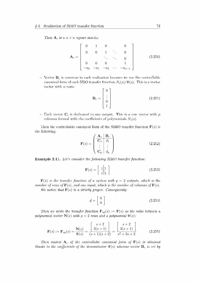
2.4. Realization of SIMO transfer function 73
Then Ac is a n× n square matrix:
Ac =
0 1 0 0
0 0 1. . . 0
. . .. . . 0
0 0 0 1−a0 −a1 −a2 · · · −an−1
(2.250)
− Vector Bc is common to each realization because we use the controllablecanonical form of each SISO transfer function Ni(s)/Ψ(s). This is a vectorvector with n rows:
Bc =
0...01
(2.251)
− Each vector Ci is dedicated to one output. This is a row vector with pcolumns formed with the coecients of polynomials Ni(s).
Then the controllable canonical form of the SIMO transfer function F(s) isthe following:
F(s) =
Ac Bc
C1 d1...
...Cp dp
(2.252)
Example 2.11. Let's consider the following SIMO transfer function:
F(s) =
[ 1s+1
2s+2
](2.253)
F(s) is the transfer function of a system with p = 2 outputs, which is thenumber of rows of F(s), and one input, which is the number of columns of F(s).
We notice that F(s) is a strictly proper. Consequently:
d =
[00
](2.254)
Then we write the transfer function Fsp(s) := F(s) as the ratio between apolynomial vector N(s) with p = 2 rows and a polynomial Ψ(s):
F(s) := Fsp(s) =N(s)
Ψ(s)=
[s+ 2
2(s+ 1)
](s+ 1)(s+ 2)
=
[s+ 2
2(s+ 1)
]s2 + 3s+ 2
(2.255)
Then matrix Ac of the controllable canonical form of F(s) is obtainedthanks to the coecients of the denominator Ψ(s) whereas vector Bc is set by

74 Chapter 2. Realization of transfer functions
the controllable canonical form:Ac =
[0 1−2 −3
]Bc =
[01
] (2.256)
Vector Cc is obtained thanks to the coecients of the polynomial vector N(s):
Cc =
[2 12 2
](2.257)
We nally get:
F(s) =
0 1 0−2 −3 1
2 1 02 2 0
(2.258)
Example 2.12. Let's consider the following SIMO transfer function:
F(s) =
[ s+1s2+6s+9
5s2+6s+9
](2.259)
F(s) is the transfer function of a system with p = 2 outputs, which is thenumber of rows of F(s), and one input, which is the number of columns of F(s).
We notice that F(s) is a strictly proper. Consequently:
d =
[00
](2.260)
Then we write the transfer function Fsp(s) := F(s) as the ratio between apolynomial vector N(s) with p = 2 rows and a polynomial Ψ(s):
F(s) := Fsp(s) =N(s)
Ψ(s)=
[s+ 1
5
]s2 + 6s+ 9
(2.261)
Then matrix Ac of the controllable canonical form of F(s) is obtainedthanks to the coecients of the denominator Ψ(s) whereas vector Bc is set bythe controllable canonical form:
Ac =
[0 1−9 −6
]Bc =
[01
] (2.262)
Vector Cc is obtained thanks to the coecients of the polynomial vector N(s):
Cc =
[1 15 0
](2.263)
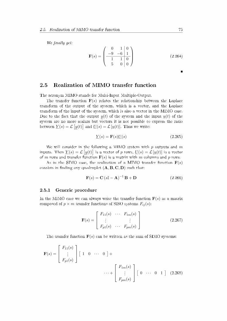
2.5. Realization of MIMO transfer function 75
We nally get:
F(s) =
0 1 0−9 −6 1
1 1 05 0 0
(2.264)
2.5 Realization of MIMO transfer function
The acronym MIMO stands for Multi-Input Multiple-Output.
The transfer function F(s) relates the relationship between the Laplacetransform of the output of the system, which is a vector, and the Laplacetransform of the input of the system, which is also a vector in the MIMO case.Due to the fact that the output y(t) of the system and the input u(t) of thesystem are no more scalars but vectors it is not possible to express the ratiobetween Y (s) = L
[y(t)
]and U(s) = L [u(t)]. Thus we write:
Y (s) = F(s)U(s) (2.265)
We will consider in the following a MIMO system with p outputs and minputs. Then Y (s) = L
[y(t)
]is a vector of p rows, U(s) = L [u(t)] is a vector
of m rows and transfer function F(s) is a matrix with m columns and p rows.
As in the SIMO case, the realization of a MIMO transfer function F(s)consists in nding any quadruplet (A,B,C,D) such that:
F(s) = C (sI−A)−1 B + D (2.266)
2.5.1 Generic procedure
In the MIMO case we can always write the transfer function F(s) as a matrixcomposed of p×m transfer functions of SISO systems Fij(s):
F(s) =
F11(s) · · · F1m(s)...
...Fp1(s) · · · Fpm(s)
(2.267)
The transfer function F(s) can be written as the sum of SIMO systems:
F(s) =
F11(s)...
Fp1(s)
[ 1 0 · · · 0]
+
· · ·+
F1m(s)...
Fpm(s)
[ 0 · · · 0 1]
(2.268)

76 Chapter 2. Realization of transfer functions
That is:
F(s) = F1(s)[
1 0 · · · 0]
+ · · ·+ Fm(s)[
0 · · · 0 1]
=∑m
i=1 Fi(s)
[0 . . . 0 1︸︷︷︸
i-th column
0 . . . 0]
(2.269)
If we realize the SIMO system Fi(s) =
F1i(s)...
Fpi(s)
in the ith column of F(s)
by
(Ai Bi
Ci Di
)then one realization of transfer function F(s) is the following:
Fi(s) =
F1i(s)...
Fpi(s)
=
(Ai Bi
Ci Di
)
⇒ F(s) =
A1 0 · · · B1 0 · · ·
0. . . 0
. . .... Am
... Bm
C1 · · · Cm D1 · · · Dm
(2.270)
The state-space representation of each SIMO transfer function Fi(s) canbe obtained thanks to the controllable canonical form (2.252). The achievedstate-space representation is block diagonal but is not necessarily minimal (seesection 2.6).
To get this result we use the same kind of demonstration than the one whichhas been to obtain the generic procedure seen in Equation (2.236). Indeed:
F(s) = F1(s)[
1 0 · · · 0]
+ · · ·+ Fm(s)[
0 · · · 0 1]
=[
F1(s) · · · Fm(s)]
=[
C1 (sI−A1)−1 B1 + D1 · · · Cm (sI−Am)−1 Bm + Dm
]=[
C1 · · · Cm
] (sI−A1)−1 B1 0 · · ·
0. . .
... (sI−Am)−1 Bm
+[
D1 · · · Dm
]
=[
C1 · · · Cm
] (sI−A1)−1 0 · · ·
0. . .
... (sI−Am)−1
B1 0 · · ·
0. . .
... Bm
+[
D1 · · · Dm
]=[
C1 · · · Cm
]
(sI−A1) 0 · · ·
0. . .
... (sI−Am)
−1
B1 0 · · ·
0. . .
... Bm
+[
D1 · · · Dm
](2.271)

2.5. Realization of MIMO transfer function 77
2.5.2 Controllable canonical form
In the MIMO case, transfer function F(s) can always be expanded as followswhere p×m constant matrices Ci, i = 1, · · · , n− 1 and D are of the same sizethan transfer function F(s) with m inputs and p outputs:
F(s) =N(s)
Ψ(s)+ D =
Cn−1sn−1 + · · ·+ C1s+ C0
1× sn + an−1sn−1 + · · ·+ a1s+ a0+ D (2.272)
Following the same procedure than in the SISO case, and by denoting Im theidentity matrix of dimension m, the controllable canonical form of F(s) reads:
F(s) =
(Ac Bc
Cc D
)(2.273)
where:
Ac =
0 Im 0 0
0 0 Im. . . 0
. . .. . . 0
0 0 0 Im−a0Im −a1Im −a2Im · · · −an−1Im
Bc =
00...0Im
Cc =
[C0 C1 · · · Cn−2 Cn−1
]D = lims→∞F(s)
(2.274)
Example 2.13. Let's consider the following transfer function:
F(s) =
[ 2s+2
s+1s+3
1s+2
5s+2
](2.275)
Let's decompose F(s) as follows:
F(s) =
[ 2s+2
−2s+3
1s+2
5s+2
]+
[0 10 0
]
=
2(s+ 3) −2(s+ 2)s+ 3 5(s+ 3)
(s+2)(s+3) +
[0 10 0
]
=
2 −21 5
s+ 6 −4
3 15
s2+5s+6
+
[0 10 0
](2.276)

78 Chapter 2. Realization of transfer functions
The system describe by transfer function F(s) has m = 2 inputs. Using(2.274) leads to the following controllable canonical realization of F(s):[
x(t)
y(t)
]=
[Ac Bc
Cc D
] [x(t)
u(t)
](2.277)
where:
Ac =
0 0 1 00 0 0 1
−6 0 −5 00 −6 0 −5
Bc =
0 00 0
1 00 1
Cc =
[6 −4 2 −23 15 1 5
]
D =
[0 10 0
]
(2.278)
This result can be checked by using Equation (2.1).
2.5.3 Diagonal (or modal) form
As in the SIMO case we expand F(s) as follows:
F(s) = Fsp(s) + D (2.279)
where D is a constant matrix and Fsp(s) a strictly proper transfer function:lims→∞F(s) = Dlims→∞Fsp(s) = 0
(2.280)
Then we have to nd matrices (A,B,C) such that:
Fsp(s) = C (sI−A)−1 B (2.281)
To get the diagonal (or modal) form we write the transfer function Fsp(s)as the sum between rational fractions. Let λ1, · · · , λr be the r distinct rootsof Ψ(s) and ni the multiplicity of root λi. Then we get the following partialfraction expansion of Fsp(s) where matrices Rij are constant:
Fsp(s) =∑i
ni∑j=1
Rij
(s− λi)j(2.282)

2.5. Realization of MIMO transfer function 79
The diagonal (or modal) form of the MIMO transfer function F(s) is thefollowing:
F(s) =
J1 0 · · · B1
0. . .
...... Jr Br
C1 · · · Cr D
(2.283)
Denoting by ni the multiplicity of the root λi, m the number of inputs ofthe system and Im the identity matrix of size m ×m, matrices Ji, Bi and Ci
are dened as follows:
− The Jordan matrix Ji is a (m× ni)× (m× ni) matrix with the followingexpression:
Ji =
λiIm Im 0 · · ·
0. . .
. . .. . .
.... . .
. . . Im0 · · · 0 λiIm
︸ ︷︷ ︸
ni termes λiIm
(2.284)
It is worth noticing that matrix (sI− Ji)−1 reads:
(sI− Ji)−1 =
(s− λi)−1Im (s− λi)−2Im · · · (s− λi)−niIm
0 (s− λi)−1Im. . . (s− λi)−ni+1Im
.... . .
. . .. . .
0 · · · 0 (s− λi)−1Im
(2.285)
− Bi is a (m× ni)×m matrix:
Bi =
0...0Im
(2.286)
− Ci is a p× (m× ni) matrix:
Ci =[
Rini · · · Ri2 Ri1
](2.287)
An alternative diagonal (or modal) form also exists. To get it rst let's focuson the realization of the following p ×m transfer function Fi(s) with a pole λof multiplicity i:
Fi(s) =
[Iρi 0ρi×(m−ρi)
0(p−ρi)×ρi 0(p−ρi)×(m−ρi)
](s− λ)i
(2.288)

80 Chapter 2. Realization of transfer functions
where Iρi is the identity matrix of dimension ρi and 0p×m the null matrixwith p rows and m columns.
Then we recall the inverse of the following n× n bidiagonal matrix:
L =
λ −1 0
λ. . .. . . −1
0 λ
⇒ L−1 =
λ−1 λ−2 · · · λ−n
λ−1 . . .. . . λ−2
0 λ−1
(2.289)
The alternative diagonal (or modal) form of Fi(s) is then the following 2:
Fi(s) =
Ai
[Bi 0nρi×(m−ρi)
][Ci
0(p−ρi)×nρi
]0p×m
(2.290)
where Ai is a (n× ρi)× (n× ρi) square matrix, BTi (the transpose of Bi) a
ρi× (n× ρi) matrix whose ρi rows are built from row vector 0 0 · · · 1︸ ︷︷ ︸n terms
and
Ci a ρi×(n×ρi) matrix whose ρi rows are built from row vector 1 0 · · · 0︸ ︷︷ ︸n terms
:
Ai =
Ji 0 · · ·
0. . .
. . ....
. . . Ji
︸ ︷︷ ︸
ρi terms
where Ji =
λ 1 0 · · ·
0. . .
. . .. . .
. . . 10 0 λ
︸ ︷︷ ︸
n terms
BTi =
0 0 · · · 1︸ ︷︷ ︸
n terms
01×n · · ·
. . .. . .
01×n · · · 0 0 · · · 1︸ ︷︷ ︸n terms
ρi terms
Ci =
1 0 · · · 0︸ ︷︷ ︸
n terms
01×n · · ·
. . .. . .
01×n · · · 1 0 · · · 0︸ ︷︷ ︸n terms
ρi terms
(2.291)
Now let's consider the following transfer function Fi(s) where Ni1 is aconstant p × ρi matrix, Ni2 a constant ρi ×m matrix and Ni1Ni2 is a p ×m
2Toshiya Morisue, Minimal Realization of a Transfer Function Matrix with Multiple Poles,Transactions of the Society of Instrument and Control Engineers, Volume 21 (1985) Issue 6Pages 546-549

2.6. Minimal realization 81
constant matrix of rank ρi:
Fi(s) =Ni1Ni2
(s− λ)i=
Ni1IρiNi2
(s− λ)iwhere rank (Ni1Ni2) = ρi (2.292)
From the preceding realization it is clear that the alternative diagonal (ormodal) form of Fi(s) is the following:
Fi(s) =
(Ai BiNi2
Ni1Ci 0p×m
)(2.293)
Finally let's consider a p×m transfer function F(s) which has pole λ withmultiplicity n and where R(s) is a matrix of polynomial of degree strictly lowerthan n. The partial fraction expansion of F(s) reads:
F(s) = R(s)(s−λ)n
= R1s−λ + R2
(s−λ)2+ · · ·+ Rn
(s−λ)n
=∑n
i=1Ri
(s−λ)i
(2.294)
Constant matrices Ri are dened by:
Ri =1
(n− i)!dn−i
dsn−i(s− λ)n F(s)
∣∣∣∣s=λ
(2.295)
Let ρi be the rank of constant matrix Ri:
ρi = rank (Ri) (2.296)
Each term Ri can be expanded as a product of two constant matrices Ni1
and Ni2 where Ni1 is a p× ρi matrix and Ni2 a ρi ×m matrix:
Ri = Ni1Ni2 = Ni1IρiNi2 (2.297)
Then the alternative diagonal (or modal) form of the MIMO transfer functionF(s) is the following:
F(s) =n∑i=1
Fi(s) + D =
A1 0 · · · B1N12
0. . .
...... An BnNn2
N11C1 · · · Nn1Cn D
(2.298)
This diagonal (or modal) form of F(s) is in general not minimal (see section2.6).
2.6 Minimal realization
2.6.1 System's dimension
Let's start with an example and consider the following transfer functions:F1(s) = 1
s+1
F2(s) = s+2s2+3s+2
(2.299)

82 Chapter 2. Realization of transfer functions
From the preceding sections it can be seen that the controllable canonicalform of transfer functions F1(s) and F2(s) are the following:
F1(s) =
(A1 B1
C1 D1
)=
(−1 1
1 0
)F2(s) =
(A2 B2
C2 D2
)=
0 1 0−2 −3 1
2 1 0
(2.300)
It is clear that the dimension of state matrix A1 is 1 and the dimension ofstate matrix A2 is 2.
On the other hand it can be seen that the poles of transfer function F2(s)are −1 and −2:
s2 + 3s+ 2 = (s+ 1)(s+ 2) (2.301)
Consequently F2(s) reads:
F2(s) =s+ 2
s2 + 3s+ 2=
s+ 2
(s+ 1)(s+ 2)=
1
s+ 1(2.302)
Thus we nally get:F2(s) = F1(s) (2.303)
Despite the fact that F2(s) = F1(s) we have obtained two realizations withdierent size of the state matrix. This usually appears when pole-zerocancellation appears in the transfer function.
The order of a realization is the size of state matrix A. So in that examplethe order of the realization of F2(s) is greater than the order of the realizationof F1(s).
This example can be extended to the general case where the dimension ofthe state matrix A corresponding to the same transfer function F(s) may vary.We said that a realization of a transfer function F(s) is minimal if there existsno realization of lesser order whose transfer function is F(s).
For SISO systems it can be proven that a realization of transfer function F(s)is minimal if and only if the two polynomials C adj(sI−A)B and det(sI−A)are coprime.
For MIMO systems it can be proven that a realization of transfer functionF(s) is minimal if and only if the characteristic polynomial of matrix A is equalto the Least Common Multiple (LCM), or Greatest Common Factor (GCF), ofthe denominators of all possible non zero minors (of all sizes) in F(s) 3.
We recall that minors or order k are the determinants of square sub-matricesof dimension k. More precisely if F(s) is a p × m matrix then the minors oforder k are obtained by computing the determinant of all the square k × ksub-matrices where p− k rows and m− k columns of F(s) have been deleted.
To nd the Least Common Multiple (LCM) of two polynomials simplyfactor each of the two polynomials completely. Then take the product of allfactors (common and not common), every factor being aected with its
3Mohammed Dahleh, Munther A. Dahleh, George Verghese, Lectures on Dynamic Systemsand Control, Massachuasetts Institute of Technology

2.6. Minimal realization 83
greatest exponent. Finally multiply the obtained polynomial by a constant toobtain a monic polynomial.
Let
(A B
C D
)be a minimal realization of a transfer function F(s). Then
the eigenvalues of A are identical to the poles of F(s). If the realization is notminimal then the poles of F(s) are a subset of the eigenvalues of A. It can beproven that Gilbert's diagonal realization is a minimal realization.
Example 2.14. Let's consider the following transfer function:
F(s) =
[ 1s+1
1s+2
2s+1
3s+1
](2.304)
A rst realization of F(s) is obtained by writing a realization of each SISOtransfer function:
F(s) =
−1 1 0−1 2 0
−2 0 1−1 0 3
1 0 1 0 0 00 1 0 1 0 0
(2.305)
The characteristic polynomial of state matrix A is:
det(sI−A) = (s+ 1)3(s+ 2) (2.306)
Whereas the Least Common Multiple (LCM) of the denominators of allpossible non zero minors (of all sizes) in F(s) is the following:
den (m11(s)) = s+ 1den (m12(s)) = s+ 2den (m21(s)) = s+ 1den (m22(s)) = s+ 1den (F(s)) = (s+ 1)2(s+ 2)
⇒ LCM = (s+ 1)2(s+ 2) (2.307)
As far as det(sI − A) 6= LCM we conclude that the realization is notminimal. Furthermore the characteristic polynomial of any state matrix of aminimal realization shall be the LCM, that is here (s+ 1)2(s+ 2).
An other realization of F(s) can be obtained by writing F(s) in diagonal (ormodal) form as explained in section 2.5.3:
F(s) =1
s+ 1
[12
] [1 0
]+
1
s+ 1
[03
] [0 1
]+
1
s+ 2
[10
] [0 1
](2.308)
Then we get:
F(s) =
−1 1 0
−1 0 1−2 0 1
1 0 1 0 02 3 0 0 0
(2.309)

84 Chapter 2. Realization of transfer functions
Because F(s) has distinct roots we can also use for this example Gilbert'srealization as explained in section 2.6.2:
F(s) =1
s+ 1R1 +
1
s+ 2R2 =
1
s+ 1
[1 02 3
]+
1
s+ 2
[0 10 0
](2.310)
− The rank of matrix R1 =
[1 02 3
]is ρ1 = 2. Thus we write R1 = C1B1
where C1 is a p× ρ1 = 2× 2 matrix and B1 is a ρ1 ×m = 2× 2 matrix.We choose for example:
C1 = R1 =
[1 02 3
]B1 = I =
[1 00 1
] (2.311)
− The rank of matrix R2 =
[0 10 0
]is ρ2 = 1. Thus we write R2 = C2B2
where C2 is a p× ρ2 = 2× 1 matrix and B2 is a ρ2 ×m = 1× 2 matrix.We choose for example: C2 =
[10
]B2 = I =
[0 1
] (2.312)
Then we get:
F(s) =
Λ1 0 B1
0 λ2 B2
C1 C2 D
=
−1 1 0
−1 0 1−2 0 1
1 0 1 0 02 3 0 0 0
(2.313)
For this example we get the same realization than (2.309).
With this realization we have det(sI−A) = LCM = (s+ 1)2(s+ 2). Thuswe conclude that this realization is minimal.
2.6.2 Gilbert's minimal realization
Let's write the p×m transfer function F(s) as follows:
F(s) = Fsp(s) + D (2.314)
where D is a constant matrix and Fsp(s) a strictly proper transfer function:lims→∞F(s) = Dlims→∞Fsp(s) = 0
(2.315)

2.6. Minimal realization 85
We consider in that section MIMO systems in which the denominatorpolynomial of the strictly proper transfer function Fsp(s) has distinct roots:
Fsp(s) =∑i
Ri
s− λi(2.316)
The residue Ri can be obtained as:
Ri = lims→λi
(s− λi) Fsp(s) = lims→λi
(s− λi) F(s) (2.317)
Now let ρi be the rank of Ri:
ρi = rank (Ri) (2.318)
and write Ri as follows where Ci is a p×ρi constant matrix and Bi a ρi×mconstant matrix:
Ri = CiBi (2.319)
Then a realization of the transfer function F(s) is the following4:
F(s) =
Λ1 0 · · · B1
0. . .
...... Λm Bm
C1 · · · Cm D
(2.320)
where matrices Λi = λiIρi are diagonal matrices of size ρi.Moreover Gilbert's realization is minimal with order n given by:
n =∑i
ρi (2.321)
2.6.3 Ho-Kalman algorithm
To get a minimal realization
(Am Bm
Cm D
)from a realization
(A B
C D
)we
can use the Ho-Kalman algorithm which is described hereafter:
− Let r be the dimension of the state matrix A, which may not be minimal.First compute the observability matrix Qo and the controllability matrix
Qc of the realization
(A B
C D
):
Qo =
C
CA...
CAr−1
Qc =
[B AB · · · Ar−1B
](2.322)
4Thomas Kailath, Linear Systems, Prentice-Hall, 1st Edition

86 Chapter 2. Realization of transfer functions
The realization is minimal if and only if:
rank (Qo) = rank (Qc) (2.323)
In all situations the dimension n of the system is given by:
n = min (rank (Qo) , rank (Qc)) (2.324)
− If the realization
(A B
C D
)is not minimal then compute the singular
value decomposition (svd) of the product QoQc:
QoQc = UΣVT (2.325)
Matrix Σ is a rectangular diagonal matrix with non-negative realcoecients situated on its diagonal. The strictly positive coecients ofΣ are called the singular values of QoQc. The number of singular valuesof QoQc (which are the strictly positive coecients within the diagonalof matrix Σ) is the dimension n of the system. Again note that n 6= r if
the realization
(A B
C D
)is not minimal.
− Let Σn be the square diagonal matrix built from the n singular valuesof QoQc (which are the non-zero coecients within the diagonal matrixΣ), Un the matrix built from the n columns of U corresponding to theaux n singular values and Vn the matrix built from the n columns of Vcorresponding to the aux n singular values:
QoQc = UΣVT =[
Un Us
] [ Σn 00 Σs
] [VTn
VTs
](2.326)
− Matrices On and Cn are dened as follows:
OnCn = UnΣnVTn where
On = UnΣ
1/2n
Cn = Σ1/2n VT
n
(2.327)
− Then the state matrix Am of a minimal realization is obtained as follows:
Am = Σ−1/2n UT
n (QoAQc) VnΣ−1/2n (2.328)
− Let m be the number of inputs of the system and p its number of outputsand Im the identity matrix of size m. Matrix Bm and Cm of the minimalrealization are obtained as follows:
Bm = Cn
Im0...
= Σ1/2n VT
n
Im0...0
Cm =
[Ip 0 · · · 0
]On =
[Ip 0 · · · 0
]UnΣ
1/2n
(2.329)
− Matrix D is independent of the realization.

Chapter 3
Analysis of Linear Time
Invariant systems
3.1 Introduction
This chapter is dedicated to the analysis of linear dynamical systems. Morespecically we will concentrate on the solution of the state equation and we willpresent the notions of controllability, observability and stability. Those notionswill enable the modal analysis of Linear Time Invariant (LTI) dynamical systems
3.2 Solving the time invariant state equation
We have seen that the state equation attached to a linear time invariant systemis the following:
x(t) = Ax(t) + Bu(t) (3.1)
The purpose of this section is to obtain the general solution of this lineardierential equation, which is actually a vector equation.
The solution of the non-homogeneous state equation x(t) = Ax(t) + Bu(t)can be obtained by the Laplace transform. Indeed the Laplace transform of thisequation yields:
sX(s)− x(0) = AX(s) + BU(s) (3.2)
That is:
(sI−A)X(s) = x(0) + BU(s) (3.3)
Pre-multiplying both sides of this equation by (sI−A)−1 leads to thefollowing equation:
X(s) = (sI−A)−1 x(0) + (sI−A)−1 BU(s) (3.4)
By taking the inverse Laplace transform of this equation we get the

88 Chapter 3. Analysis of Linear Time Invariant systems
expression of the state vector x(t):
x(t) = L−1 [X(s)]
= L−1[(sI−A)−1 x(0) + (sI−A)−1 BU(s)
]= L−1
[(sI−A)−1
]x(0) + L−1
[(sI−A)−1 BU(s)
] (3.5)
To inverse the preceding equation in the s domain and come back in thetime domain we will use the following properties of the Laplace transform:
− Convolution theorem: let x(t) and y(t) be two causal scalar signals anddenote by X(s) and Y (s) their Laplace transforms, respectively. Then theproduct X(s)Y (s) is the Laplace transform of the convolution betweenx(t) and y(t) which is denoted by x(t) ∗ y(t):
X(s)Y (s) = L [x(t) ∗ y(t)]⇔ L−1 [X(s)Y (s)] = x(t) ∗ y(t) (3.6)
Where:
x(t) ∗ y(t) =
∫ t
0x(t− τ)y(τ)dτ (3.7)
This relationship is readily extended to the vector case where X(t) is amatrix and y(t) a vector:
L−1 [X(s)Y (s)] = X(t) ∗ y(t) =
∫ t
0X(t− τ)y(τ)dτ (3.8)
− Laplace transform of exponential matrix: in the scalar case we have seenthat:
L[eat]
=1
s− a= (s− a)−1 ⇔ L−1
[(s− a)−1
]= eat (3.9)
This relationship is readily extended to the vector case as follows:
L[eAt]
= (sI−A)−1 ⇔ L−1[(sI−A)−1
]= eAt (3.10)
Thus the inverse Laplace transform of Equation (3.5) leads to the expressionof the state vector x(t) which solves the state equation (3.1):
x(t) = eAtx(0) +
∫ t
0eA(t−τ)Bu(τ)dτ (3.11)
The solution x(t) of Equation (3.5) is often referred to as the state trajectoryor the system trajectory.
Exponential eAt is dened as the transition matrix Φ(t):
Φ(t) = eAt (3.12)
In the more general case of time dependent linear dierential equation ofthe form x(t) = A(t)x(t) + B(t)u(t) the expression of the state vector is x(t) =Φ(t, t0)x(0) +
∫ tt0
Φ(t, τ)Bu(τ)dτ where Φ(t, t0) is also named the transition

3.3. Output response 89
matrix (or Green's matrix). In this case the transition matrix is a solution of
the homogeneous equation ∂Φ(t,t0)∂t = A(t)Φ(t, t0). In addition Φ(t, t) = I ∀t
and Φ(t, t0) = φ(t)φ−1(t0) where φ(t) is the solution of x(t) = A(t)x(t). For alinear time invariant system the transition matrix Φ(t, t0) is Φ(t, t0) = eA(t−t0);as far as for the time invariant case the initial time t0 is meaningless we canchoose t0 = 0 and we retrieve Φ(t) = eAt.
3.3 Output response
We have seen that the output vector y(t) of the state space representation isobtained thanks to the output equation. Using the expression of the state vectorx(t) we get:
y(t) = Cx(t) + Du(t)
= C(eAtx(0) +
∫ t0 e
A(t−τ)Bu(τ)dτ)
+ Du(t)
= CeAtx(0) +∫ t
0 CeA(t−τ)Bu(τ)dτ + Du(t)
(3.13)
− The term CeAtx(0) is called the zero-input response (or output) of thesystem; this is the response of the system when there is no input signalu(t) applied on the system;
− The term∫ t
0 CeA(t−τ)Bu(τ)dτ + Du(t) is called the zero-state output (orresponse) of the system; this is the response of the system when there isno initial condition x(0) applied on the system.
3.4 Impulse and unit step responses
The impulse response of a dynamical system is the zero-state output of thesystem when the input signal u(t) is the impulse δ(t) called the Dirac deltafunction.
Setting in (3.13) the input signal u(t) to the Dirac delta function δ(t) andputting the initial conditions x(0) to zero leads to the following expression ofthe impulse response of the system:
y(t) =
∫ t
0CeA(t−τ)Bδ(τ)dτ + Dδ(t) (3.14)
The term∫ t
0 CeA(t−τ)Bδ(τ)dτ can be expressed as the convolution betweenthe matrix CeAtB and the input vector δ(τ). We get:
y(t) = CeAtB ∗ δ(t) + Dδ(t) (3.15)
Using the fact that the Dirac delta function δ(t) is the neutral element forconvolution we can write CeAtB ∗ δ(t) = CeAtB. Consequently the outputvector y(t), that is the impulse response of a linear time invariant system whichwill be denoted h(t), can be expressed as follows:
y(t) := h(t) = CeAtB + Dδ(t) (3.16)

90 Chapter 3. Analysis of Linear Time Invariant systems
The Laplace transform of the impulse response h(t) is dened to be thetransfer function F(s) of the system. Using the fact that the Laplace transformof the Dirac delta function δ(t) is 1 we retrieve the following expression for thetransfer function F(s) of the linear system:
F(s) = L [h(t)] = C (sI−A)−1 B + D (3.17)
The unit step response is the response of the system to the unit step input.Setting in (3.13) the input signal u(t) to u(t) = 1 ∀t > 0 and putting the initialconditions x(0) to zero leads to the following expression of the unit step responseof the system:
y(t) =∫ t
0 CeA(t−τ)Bdτ + D1
= CeAt(∫ t
0 e−Aτdτ
)B + D1
= CeAt(−A−1e−Aτ
∣∣tτ=0
)B + D1
= CeAt(A−1 −A−1e−At
)B + D1
(3.18)
Using the fact that eAtA−1 = A−1eAt (which is easy to show using theseries expansion of eAt) and assuming that matrix A−1 exists, we nally get thefollowing expression for the unit step response of the system:
y(t) = CA−1(eAt − I
)B + D1 (3.19)
3.5 Matrix exponential
3.5.1 Denition
Let A be a n×n square matrix. The matrix exponential is a n×n matrix whichis dened by analogy with the scalar exponential and its series as follows:
eAt =∞∑k=0
(At)k
k!= I +
∞∑k=1
(At)k
k!(3.20)
This calculus involves an innity of terms and it is in general impossible tocompute it by hand except for some specic cases, for example if matrix A isnilpotent.
A matrix A is nilpotent if there exists an integer k such that Ak = 0. Thesmallest value of k is called the index of nilpotency (of the nilpotent matrix). Inthis case the matrix exponential eAt can be computed directly from the seriesexpansion as the series terminates after a nite number of terms:
eAt = I + At+ A2 t2
2!+ · · ·+ Ak−1 tk−1
(k − 1)!(3.21)
A necessary and sucient condition for a n × n square matrix A to benilpotent is that its characteristic polynomial det (sI−A) is equal to sn:
Ak = 0⇔ det (sI−A) = sn where k ≤ n (3.22)

3.5. Matrix exponential 91
We recall that the minimal polynomial πA(s) of a matrix A is the monicpolynomial (a monic polynomial is a polynomial in which the leading coecient(the nonzero coecient of highest degree) is equal to 1) of least degree suchthat πA(A) = 0. The minimal polynomial divides the characteristic polynomialχA(s) := det (sI−A) of matrix A. Consequently its degree is lower or equal tothe order n of matrix A.
A matrix A is said to be cyclic if and only if its characteristic polynomial isthe same than its minimal polynomial.
Furthermore matrix A is diagonalizable if and only if its minimalpolynomial's roots are all of multiplicity one.
The previous result to compute eAt when A is nilpotent can be generalizedto the case where the minimal polynomial πA(s) of A reads (s− λ)k. Indeedwe get in this case:
πA(s) = (s− λ)k ⇒ (A− λI)k = 0 (3.23)
Thus matrix A− λI is nilpotent and we can write:
e(A−λI)t = I + (A− λI) t+ (A− λI)2 t2
2!+ · · ·+ (A− λI)k−1 tk−1
(k − 1)!(3.24)
As soon as matrices A and λI commute the following relationship holds:
e(A−λI)t = e−λteAt ⇒ eAt = eλt e(A−λI)t (3.25)
Thus as soon as πA(s) = (s− λ)k we nally get the following result:
eAt =
eλt(I + (A− λI) t+ (A− λI)2 t
2
2!+ · · ·+ (A− λI)k−1 tk−1
(k − 1)!
)(3.26)
Example 3.1. Let A =
[0 10 0
]. The characteristic polynomial of A is:
det (sI−A) = det
([s −10 s
])= s2 (3.27)
Consequently matrix A is nilpotent and eAt can be computed as follows:
A =
[0 10 0
]⇒ A2 =
[0 00 0
]⇒ eAt = I + At =
[1 t0 1
] (3.28)

92 Chapter 3. Analysis of Linear Time Invariant systems
3.5.2 Properties
The following properties hold 1:
− Value at t = 0:eAt∣∣t=0
= e0 = I (3.29)
− Derivation:d
dteAt = AeAt = eAtA (3.30)
− Integration:
eAt = I + A
∫ t
0eAτdτ (3.31)
− In general:e(A+B)t 6= eAteBt 6= eBteAt (3.32)
Nevertheless if matrices A and B commute (meaning that AB = BA)then:
e(A+B)t = eAteBt = eBteAt (3.33)
As far as the product AA commutes we have:
eAteAτ = eA(t+τ) = eAτeAt (3.34)
And thus setting τ to −t we get:(eAt)−1
= e−At (3.35)
− Let λ(A) be the eigenvalues of matrix A. Then:
λ(eAt)
= eλ(A)t (3.36)
− Let det (A) be the determinant of matrix A and tr (A) be the trace ofmatrix A. Then:
det(eAt)
= etr(A)t (3.37)
Example 3.2. Let's consider the following matrices A and B:A =
[0 10 0
]
B =
[1 00 0
] (3.38)
It is clear that A et B do not commute. Indeed:
AB =
[0 00 0
]6= BA =
[0 10 0
](3.39)
1https://en.wikipedia.org/wiki/Matrix_exponential

3.5. Matrix exponential 93
Consequently we expect that eAteBt 6= eBteAt. We will check it by using thepreceding denitions and properties:
eAt =
[1 t0 1
](3.40)
And:
(Bt)k =
[tk 00 0
]⇒ eBt = I +
∑∞k=1
(Bt)k
k! =
[1 +
∑∞k=1
tk
k! 00 1
]⇔ eBt =
[et 00 1
] (3.41)
It is clear that:
eAteBt =
[et t0 1
]6= eBteAt =
[et tet
0 1
](3.42)
We can also easily check the following properties:ddte
At = AeAt = eAtA =
[0 10 0
]ddte
Bt = BeBt = eBtB =
[et 00 0
] (3.43)
3.5.3 Computation of eAt thanks to the diagonal form of A
We will assume in that section that matrix A is diagonalizable or equivalentlythat matrix A has linearly independent eigenvectors; this means that for alleigenvalues λi of A the rank of matrix λiI−A is equal to the size of A minusthe multiplicity of λi.
Assuming that matrix A is diagonalizable then there exists a similaritytransformation such that:
A = PΛP−1 where Λ =
λ1
. . .
λn
(3.44)
The change of basis matrix P, as well as its inverse P−1, can be obtained asfollows:
− Let vi be the eigenvector of A corresponding to eigenvalue λi. As far asthe n×n matrix A is assumed to have n linearly independent eigenvectorswe can write:
Av1 = λ1v1...Avn = λnvn
(3.45)

94 Chapter 3. Analysis of Linear Time Invariant systems
− The preceding relationship can be written in a vector form as follows:
A[v1 . . . vn
]=[v1 . . . vn
] λ1
. . .
λn
(3.46)
− Identifying the preceding equation with AP = PΛ we nally get
P =[v1 v2 · · · vn
](3.47)
− Furthermore let wi be the eigenvectors of matrix AT :
ATwj = λjwj ⇔ wTj A = λjwTj (3.48)
It can be seen that vectors wj et vi are orthogonal. Indeed:
λjwTj vi = wTj Avi = wTj λivi ⇔ (λi − λj)wTj vi = 0
⇒ wTj vi = 0 si j 6= i(3.49)
Thus imposing wTi vi = 1 ∀i, the inverse of matrix P is obtained as follows:
wTi vi = 1 ∀i⇒ P−1 =
wT1wT2...wTn
(3.50)
Indeed using wTj vi =
0 if j 6= i1 if j = i
we get:
P−1P =
wT1wT2...wTn
[ v1 v2 · · · vn]
=
wT1 v1 wT1 v2 · · · wT1 vnwT2 v1 wT2 v2 · · · wT2 vn...
......
wTnv1 wTnv2 · · · wTnvn
=
1 0 · · · 00 1 · · · 0...
. . ....
0 0 · · · 1
= I
(3.51)
Then, as soon as matrix A diagonalizable, eAt can be obtained thanks tothe following relationship :
eAt = PeΛtP−1 =n∑i=1
viwTi e
λit (3.52)

3.5. Matrix exponential 95
The preceding relationship is easily obtained by using the series developmentof the exponential:
ePΛtP−1=
∞∑k=0
(PΛtP−1
)kk!
=
∞∑k=0
P (Λt)k P−1
k!= P
( ∞∑k=0
(Λt)k
k!
)P−1 (3.53)
As far as the diagonal (or modal) matrix Λ is diagonal we get:Λk =
λk1. . .
λkn
eΛt =
∑∞k=0
(Λt)k
k!
⇒ eΛt =
eλ1t
. . .
eλnt
(3.54)
Thus using the expression of P and P−1:
eAt = PeΛtP−1 = P
eλ1t
. . .
eλnt
P−1
=[v1 v2 · · · vn
] eλ1t
. . .
eλnt
wT1wT2...wTn
(3.55)
We nally get:
eAt =n∑i=1
vieλitwTi =
n∑i=1
viwTi e
λit (3.56)
Example 3.3. Compute eAt where A =
[1 20 −5
].
Le characteristic polynomial of A reads:
det (sI−A) = det
([s− 1 −2
0 s+ 5
])= (s− 1)(s+ 5) (3.57)
The two eigenvalues λ1 = 1 and λ2 = −5 of A are distinct. Since the sizeof A is equal to the number of the distinct eigenvalues we conclude that matrixA is diagonalizable.
− Let v1 =
[v11
v12
]be the eigenvector of A corresponding to λ1 = 1. We
have: [1 20 −5
] [v11
v12
]= 1×
[v11
v12
]⇔v11 + 2v12 = v11
−5v12 = v12
⇒ v12 = 0
(3.58)
Thus the expression of eigenvector v1 is:
v1 =
[v11
0
](3.59)

96 Chapter 3. Analysis of Linear Time Invariant systems
− Let v2 =
[v21
v22
]be the eigenvector of A corresponding to λ2 = −5. We
have: [1 20 −5
] [v21
v22
]= −5×
[v21
v22
]⇔v21 + 2v22 = −5v21
−5v22 = −5v22
⇒ 6v21 + 2v22 = 0⇔ v22 = −3v21
(3.60)
Thus the expression of eigenvector v2 is:
v2 =
[v21
−3v21
](3.61)
− Let w1 =
[w11
w12
]be the eigenvector of AT corresponding to λ1 = 1. We
have: [1 02 −5
] [w11
w12
]= 1×
[w11
w12
]⇔w11 = w11
2w11 − 5w12 = w12
⇒ 2w11 − 6w12 = 0⇔ w11 = 3w12
(3.62)
Thus the expression of eigenvector w1 is:
w1 =
[3w12
w12
](3.63)
It is clear that w1 and v2 are orthogonal:
wT1 v2 =[
3w12 w12
] [ v21
−3v21
]= 0 (3.64)
− Let w2 =
[w21
w22
]be the eigenvector of AT corresponding to λ2 = −5. We
have: [1 02 −5
] [w21
w22
]= −5×
[w21
w22
]⇔w21 = −5w21
2w21 − 5w22 = −5w22
⇒ w21 = 0
(3.65)
Thus the expression of eigenvector w2 is:
w2 =
[0w22
](3.66)
It is clear that w2 and v1 are orthogonal:
wT2 v1 =[
0 w22
] [ v11
0
]= 0 (3.67)

3.5. Matrix exponential 97
Finally v1, v2, w1 and w2 are chosen such that wT1 v1 = wT2 v2 = 1. We canchose for example:
v1 =
[v11
0
]=
[10
]and w1 =
[3w12
w12
]=
[113
](3.68)
And:
v2 =
[v21
−3v21
]=
[−1
31
]and w2 =
[0w22
]=
[01
](3.69)
Then applying Equation (3.52) we get:
eAt =∑n
i=1 viwTi e
λit
= v1wT1 e
λ1t + v2wT2 e
λ2t
=
[10
]et[
1 13
]+
[−1
31
]e−5t
[0 1
]=
[1 1
30 0
]et +
[0 −1
30 1
]e−5t
=
[et 1
3et − 1
3e−5t
0 e−5t
](3.70)
We can check that eAt∣∣t=0
= I.
3.5.4 Computation of eAt thanks to the Laplace transform
Computation of eAt can be done thanks to the Laplace transform. Denoting byL the Laplace transform and by L−1 the inverse Laplace transform we have thefollowing property which extends to the vector case a well-known result in thescalar case:
L[eAt]
= (sI−A)−1 ⇔ eAt = L−1[(sI−A)−1
]∀ t ≥ 0 (3.71)
Matrix (sI−A)−1 is called the resolvent of matrix A. It can be computedthanks to the Faddeev-Leverrier's method for example (see section 1.6).
The inverse Laplace transform is taken for each term of the resolvent ofmatrix A. We recall that the inverse Laplace transform of a strictly properrational fraction F (s) (i.e. the degree of the denominator is strictly greater thanthe degree of the denominator) can be obtained thanks to the Mellin-Fourierintegral.
The Mellin-Fourier integral reads:
g(t) = L−1 [F (s)] =∑
poles of F (s)
Res[F (s)est
]∀t ≥ 0 (3.72)
The residue Res[F (s)est
]shall be computed around each pole of F (s).
Assuming that λk is a pole of multiplicity nk then the residue of F (s) aroundpole λk is given by:
Ress=λk[F (s)est
]=
1
(nk − 1)!
dnk−1
dsnk−1(s− λk)nk F (s)est
∣∣∣∣s=λk
(3.73)

98 Chapter 3. Analysis of Linear Time Invariant systems
Alternatively if resolvent of matrix A is decomposed as N(s)Ψ(s) where degree
of polynomial matrix N(s) is strictly lower than degree of polynomial Ψ(s) =∏k(s − λk)
nk then the use of Mellin-Fourier integral leads to the followingexpression of eAt:
(sI−A)−1 = N(s)Ψ(s) = N(s)∏
k(s−λk)nk
⇒ eAt =∑
k1
(nk−1)!dnk−1
dsnk−1 (s− λk)nk N(s)Ψ(s) e
st∣∣∣s=λk
(3.74)
Example 3.4. Compute eAt where:
A =
[0 10 0
](3.75)
Here n = 2 and the Faddeev-Leverrier's method (see section 1.6) reads:
F0 = Id1 = tr (AF0) = tr (A) = 0 and F1 = AF0 − d1I = Ad2 = 1
2 tr (AF1) = 12 tr
(A2)
= 0and det (sI−A) = s2 − d1s− d2 = s2
(3.76)
Thus:
(sI−A)−1 =1
det (sI−A)(F0s+ F1) =
1
s2
[s 10 s
]=
[1s
1s2
0 1s
](3.77)
Then we have to apply the Mellin-Fourier integral as well as the residuetheorem on each term of the resolvent matrix of A:
L−1[
1s
]= Res
[1sest]s=0
= 1(1−1)!
d1−1
ds1−1 s1sest∣∣∣s=0
= est∣∣s=0
= 1
L−1[
1s2
]= Res
[1s2est]s=0
= 1(2−1)!
d2−1
ds2−1 s2 1s2est∣∣∣s=0
= test∣∣s=0
= t(3.78)
We nally get:
exp
([0 10 0
]t
)= L−1
[1s
1s2
0 1s
]=
[1 t0 1
](3.79)
Alternatively resolvent of matrix A can be decomposed as N(s)Ψ(s) . Indeed we
have seen that:
(sI−A)−1 =1
s2
[s 10 s
](3.80)

3.5. Matrix exponential 99
The use of Mellin-Fourier integral leads to the following expression of eAt:
(sI−A)−1 = N(s)Ψ(s)
⇒ eAt =∑
k1
(nk−1)!dnk−1
dsnk−1 (s− λk)nk N(s)Ψ(s) e
st∣∣∣s=λk
= 1(2−1)!
d2−1
ds2−1 s2 1s2
[s 10 s
]est∣∣∣∣s=0
= dds
[s 10 s
]est∣∣∣∣s=0
=
[1 00 1
]est∣∣∣∣s=0
+
[s 10 s
]t est
∣∣∣∣s=0
=
[1 00 1
]+
[0 10 0
]t
=
[1 t0 1
]
(3.81)
Example 3.5. Compute eAt where:
A =
[1 10 0
](3.82)
We have:
(sI−A)−1 =
([s− 1 −1
0 s
])−1
=1
s(s− 1)
[s 10 s− 1
](3.83)
Thus (sI−A)−1 = N(s)Ψ(s) where Ψ(s) = s(s − 1) has two roots, λ1 = 0 and
λ2 = 1, each of multiplicity 1: n1 = n2 = 1.The use of Mellin-Fourier integral leads to the following expression of eAt:
(sI−A)−1 = N(s)Ψ(s)
⇒ eAt =∑
k1
(nk−1)!dnk−1
dsnk−1 (s− λk)nk N(s)Ψ(s) e
st∣∣∣s=λk
= 1(1−1)!
d1−1
ds1−1 s1
s(s−1)
[s 10 s− 1
]est∣∣∣∣s=0
+ 1(1−1)!
d1−1
ds1−1 (s− 1) 1s(s−1)
[s 10 s− 1
]est∣∣∣∣s=1
= 1s−1
[s 10 s− 1
]est∣∣∣∣s=0
+ 1s
[s 10 s− 1
]est∣∣∣∣s=1
=
[0 −10 1
]+
[1 10 0
]et
=
[et et − 10 1
]
(3.84)
Example 3.6. Compute eAt where:
A =
[1 20 −5
](3.85)

100 Chapter 3. Analysis of Linear Time Invariant systems
Here n = 2 and the Faddeev-Leverrier's method (see section 1.6) reads:F0 = I
d1 = tr (AF0) = −4 and F1 = AF0 − d1I =
[5 20 −1
]d2 = 1
2 tr (AF1) = 12 tr
([5 00 5
])= 5
and det (sI−A) = s2 − d1s− d2 = s2 + 4s− 5 = (s− 1)(s+ 5)
(3.86)
Thus:
(sI−A)−1 = 1det(sI−A) (F0s+ F1) = 1
(s−1)(s+5)
[s+ 5 2
0 s− 1
]⇔ (sI−A)−1 =
[1s−1
2(s−1)(s+5)
0 1s+5
] (3.87)
Then we have to apply the Mellin-Fourier integral as well as the residuetheorem on each term of the resolvent matrix of A:
L−1[
1s−1
]= et
L−1[
1s+5
]= e−5t
L−1[
2(s−1)(s+5)
]= 2
(16et − 1
6e−5t)
= 13et − 1
3e−5t
(3.88)
We nally get:
exp
([1 20 −5
]t
)= L−1
[1s−1
2(s−1)(s+5)
0 1s+5
]=
[et 1
3et − 1
3e−5t
0 e−5t
] (3.89)
Alternatively resolvent of matrix A can be decomposed as N(s)Ψ(s) . Indeed we
have seen that:
(sI−A)−1 =1
(s− 1)(s+ 5)
[s+ 5 2
0 s− 1
](3.90)
The use of Mellin-Fourier integral leads to the following expression of eAt:
(sI−A)−1 = N(s)Ψ(s)
⇒ eAt =∑
k1
(nk−1)!dnk−1
dsnk−1 (s− λk)nk N(s)Ψ(s) e
st∣∣∣s=λk
= (s− 1) 1(s−1)(s+5)
[s+ 5 2
0 s− 1
]est∣∣∣∣s=1
+ (s+ 5) 1(s−1)(s+5)
[s+ 5 2
0 s− 1
]est∣∣∣∣s=−5
=
[1 1
30 0
]est∣∣∣∣s=1
+
[0 −1
30 1
]est∣∣∣∣s=−5
=
[et 1
3et
0 0
]+
[0 −1
3e−5t
0 e−5t
]=
[et 1
3et − 1
3e−5t
0 e−5t
]
(3.91)

3.6. Stability 101
Example 3.7. Compute eAt where:
A =
2 −1 00 1 01 −1 1
(3.92)
From the Faddeev-Leverrier's method (see section 1.6) we get:
(sI−A)−1 =
1s−2
−1(s−1)(s−2) 0
0 1s−1 0
1(s−1)(s−2)
−1(s−1)(s−2)
1s−1
(3.93)
Then we have to apply the Mellin-Fourier integral as well as the residuetheorem on each term of the resolvent matrix of A:
L−1[
1s−2
]= e2t
L−1[
1s−1
]= et
L−1[
1(s−1)(s−2)
]= e2t − et
(3.94)
We nally get:
eAt =
e2t et − e2t 00 et 0
e2t − et et − e2t et
(3.95)
3.6 Stability
There are two dierent denitions of stability: internal stability and input-output stability:
− A linear time-invariant system is internally stable if its the zero-input stateeAtx0 moves towards zero for any initial state x0;
− A linear time-invariant system is input-output stable if its zero-stateoutput is bounded for all bounded inputs; this type of stability is alsocalled Bounded-Input Bounded-Output (BIBO) stability.
We have seen in (3.13) that the output response y(t) of a linear time-invariantsystem is the following:
y(t) = CeAtx0 +
∫ t
0CeA(t−τ)Bu(τ)dτ + Du(t) (3.96)
Assuming that matrix A is diagonalizable, we have seen in (3.52) that eAt
can be obtained thanks to the following relationship :
eAt = PeΛtP−1 =n∑i=1
viwTi e
λit (3.97)
Thus;

102 Chapter 3. Analysis of Linear Time Invariant systems
− The zero-input state, which is obtained when u(t) = 0, has the followingexpression:
x(t) = eAtx0 =
n∑i=1
viwTi e
λitx0 (3.98)
Consequently the zero-input state moves towards zero for any initial statex0 as soon as all the eigenvalues λi of matrix A are situated in the openleft-half plane (they have strictly negative real part). This means that alinear time-invariant system is internally stable when all the eigenvaluesλi of matrix A are situated in the open left-half plane (i.e. they havestrictly negative real part).
The result which have been shown assuming that matrix A isdiagonalizable can be extended to the general case where matrix A isnot diagonalizable; in that situation this is the Jordan form of A whichleads to the same result concerning internal stability.
− The zero-state output, which is obtained when x0 = 0, has the followingexpression:
y(t) =∫ t
0 CeA(t−τ)Bu(τ)dτ + Du(t)
=(CeAtB + Dδ(t)
)∗ u(t)
(3.99)
It can be shown that the zero-state output is bounded if and only all thepoles of each term of the transfer function F(s) are situated in the openleft-half plane (i.e. they have strictly negative real part):
F(s) = L[CeAtB + Dδ(t)
]= C (sI−A)−1 B + D (3.100)
The two types of stability are related. Indeed:
− If a linear time invariant system is internally stable it is also input-output(or BIBO) stable because all the poles of the transfer function F(s) areeigenvalues of matrix A;
− Nevertheless the converse is not true since matrix A could have unstablehidden modes which do not appear in the poles of F(s). Indeed there maybe pole-zero cancellation while computing F(s). Thus a system may beBIBO stable even when some eigenvalues of A do not have negative realpart.
Example 3.8. Let's consider the following realization:
(A B
C D
)=
−1 10 −20 1 0
−2 3 −2
(3.101)
Matrix A has a stable mode, which is −1, and an unstable mode, which is1. Thus the system is not internally stable.

3.7. Controllability 103
When computing the transfer function of the system we can observe a pole/ zero cancellation of the unstable mode:
F (s) = C (sI−A)−1 B + D
=[−2 3
] [ 1s+1
10s2−1
0 1s−1
] [−20
]− 2
= 4s+1 − 2
= −2s+2s+1
(3.102)
The pole of the transfer function F (s) is −1. Thus the system is BIBO stablebut not internally stable.
3.7 Controllability
3.7.1 Denition
Let's consider the state trajectory x(t) of a linear time-invariant system:
x(t) = eAtx0 +
∫ t
0eA(t−τ)Bu(τ)dτ (3.103)
Where A is a n× n real matrix and B is a n×m real matrix.
Controllability answers the question whether it is possible to control thestate vector x(t) through an appropriate choice of the input signal u(t).
More precisely an initial state x0 is said controllable if and only if thereexists an input signal u(t) which is able to move the state vector x(t) from aninitial state x(0) = x0 at t = 0 to the origin x(tf ) = 0 in a nite time tf . Wesaid that a system is controllable when any arbitrary initial state x0 ∈ Rn iscontrollable 2.
If the system is controllable then the input signal u(t) which is able to movethe state vector x(t) from an initial state x(0) = x0 at t = 0 to the originx(tf ) = 0 in a nite time tf reads3:
u(t) = −BT eAT (tf−t) W−1
c (tf )eAtf x0 (3.104)
Where Wc(tf ) is a symmetric matrix dened as follows:
Wc(tf ) =
∫ tf
0eAτBBT eA
T τdτ (3.105)
2https://en.wikibooks.org/wiki/Control_Systems/Controllability_and_Observability3S. Skogestad and I. Postlethwaite: Multivariable Feedback Control Analysis and design,
Wiley, 1996; 2005

104 Chapter 3. Analysis of Linear Time Invariant systems
Indeed when x(tf ) is computed with this control we get x(tf ) = 0:
x(tf ) = eAtfx0 +∫ tf
0 eA(tf−τ)Bu(τ)dτ
= eAtfx0 −∫ tf
0 eA(tf−τ)BBT eAT (tf−τ) W−1
c (tf )eAtf x0 dτ
= eAtfx0 +(∫ 0
tfeAvBBT eA
T v dv)
W−1c (tf )eAtf x0
= eAtfx0 −(∫ tf
0 eAτBBT eAT τ dτ
)W−1
c (tf )eAtf x0
= eAtfx0 −Wc(tf )W−1c (tf )eAtf x0
= 0
(3.106)
More generally one can verify that a particular input which achieves x(tf ) =xf is given by3:
u(t) = −BT eAT (tf−t) W−1
c (tf )(eAtf x0 − xf
)(3.107)
Consequently a system is controllable if and only if symmetric matrix Wc(tf )is nonsingular for any tf > 0. Furthermore Wc(t) is the solution of the followingdierential equation:
AWc(t) + Wc(t)AT + BBT =
d
dtWc(t) (3.108)
If all eigenvalues of matrix A have negative real parts (A is said to beHurwitz ) then Wc(t) tends towards a constant matrix as t → ∞. Thecontrollability Gramian Wc is the following positive denite symmetricmatrix:
Wc =
∫ ∞0
eAτBBT eAT τdτ (3.109)
It can be shown that Wc is the unique solution of the following Lyapunovequation:
AWc + WcAT + BBT = 0 (3.110)
3.7.2 Use of the diagonal form: Gilbert's criteria
Assuming that all eigenvalues are distinct, controllability property can be readilyanalyzed by inspecting the null rows of the input matrix B as soon as we getthe modal (or diagonal) form of the state space representation.
Indeed we have seen in the the chapter dedicated to the state-spacerepresentation that for a single input system matrices A and B of the stateequation x(t) = Ax(t) + Bu(t) read as follows assuming that matrix A has n

3.7. Controllability 105
independent eigenvectors :
A =
λ1 0 0
0 λ2...
.... . . 0
0 · · · 0 λn
B =
b1b2...bn
(3.111)
Thus in the time domain the diagonal form of the state space representationx(t) = Ax(t) + Bu(t) reads:
x1(t) = λ1x1(t) + b1u(t)x2(t) = λ2x2(t) + b2u(t)...xn(t) = λnxn(t) + bnu(t)
(3.112)
Consequently if at least one of the bi's coecients is zero then the statecomponent xi(t) is independent of the input signal u(t) and the state isuncontrollable.
For multi inputs system with m inputs then matrix B has m columns andthe preceding analysis is readily extended to each column of matrix B assumingthat the state space representation is the diagonal form.
Gilbert's controllability criteria (1963) states that a multi inputs systemwith distinct eigenvalues is controllable if and only if each row of control matrixB of the diagonal realization (all eigenvalues are distinct) has at least one nonzero element.
3.7.3 Popov-Belevitch-Hautus (PBH) test
There exists another test for controllability which is called the Popov-Belevitch-Hautus (PBH) test.
Popov-Belevitch-Hautus (PBH) test indicates that a linear system iscontrollable when the rank of matrix
[A− λiI B
]is equal to n for all
eigenvalues λi of matrix A.A linear system is stabilizable when the rank of matrix
[A− λiI B
]is
equal to n for all unstable eigenvalues λi of matrix A.Eigenvalues λi for which rank of matrix
[A− λiI B
]is not equal to n
are said uncontrollable.
Example 3.9. Let's consider the following realization:
(A B
C D
)=
−1 10 −20 1 0
−2 3 −2
(3.113)

106 Chapter 3. Analysis of Linear Time Invariant systems
Matrix A has two modes, λ1 = −1 and λ2 = 1.Let's apply the PBH test for λ1 = −1:
rank[
A− λ1I B]
= rank
[0 10 −20 2 0
]= 2 (3.114)
We conclude that the mode λ1 = −1 is controllable.Let's apply the PBH test for λ2 = 1:
rank[
A− λ2I B]
= rank
[−2 10 −20 0 0
]= 1 6= 2 (3.115)
We conclude that the mode λ2 = 1 is not controllable.
3.7.4 Kalman's controllability rank condition
Let Qc be the controllability matrix. Matrix Qc is dened as follows:
Qc =[
B AB · · · An−1B]
(3.116)
It can be shown that a linear system is controllable if and only if the rank ofthe controllability matrix Qc is equal to n. This is the Kalman's controllabilityrank condition.
The sketch of the demonstration is the following:
− First we recall that the expression of the state vector x(t) at time t = tfwhich solves the state equation (3.1) is:
x(tf ) = eAtfx0 +
∫ tf
0eA(tf−τ)Bu(τ)dτ (3.117)
As far as x0, tf and x(tf ) are assumed to be known we rewrite thepreceding equation as follows:
e−Atfx(tf )− x0 =
∫ tf
0e−AτBu(τ)dτ (3.118)
− To continue the sketch of the proof we need the CayleyHamilton theorem.Let χA(s) be the characteristic polynomial of the n × n matrix A. Wewrite the characteristic polynomial χA(s) of matrix A as follows:
χA(s) := det(sI−A) = sn + an−1sn−1 + · · ·+ a1s+ a0 (3.119)
The CayleyHamilton theorem states that substituting matrix A for s inthe characteristic polynomial χA(s) of matrix A results in the zero matrix4:
χA(A) = 0 = An + an−1An−1 + · · ·+ a1A + a0I (3.120)
4https://en.wikipedia.org/wiki/CayleyHamilton_theorem

3.7. Controllability 107
From the preceding equation it is clear that we can express An as afunction of Ak where 0 ≤ k ≤ n− 1:
An = −an−1An−1 − · · · − a1A− a0I (3.121)
More generally this relationship allows to replace a term of the form Am
where m ≥ n by a linear combination of Ak where 0 ≤ k ≤ n− 1. Whenwe use this property to replace the terms Am where m ≥ n in the seriesexpansion of eAt we get the following relationship:
eAt =∑∞
k=0(At)k
k! =∑n−1
k=0Aktk
k! +∑∞
k=nAktk
k!An = −an−1A
n−1 − · · · − a1A− a0IAm =
∑n−1i=0 αiA
i ∀m ≥ n(3.122)
Consequently the series expansion of eAt can be cut so that no power ofmatrix A greater that n appears in the series expansion:
eAt =n−1∑k=0
γk(t)Ak (3.123)
where γk(t) are functions of time t. As far as det(sI − A) is equal tozero when s = λi is an eigenvalue of matrix A the preceding matrixrelationship is also be obtained for all the eigenvalues of matrix A. Weobtain the following relationship which is satised by the functions γk(t):
eλit =n−1∑k=0
γk(t)λki (3.124)
− Using (3.123) and the fact that functions γk(t) are scalar functions (3.118)is rewritten as follows:
e−Atfx(tf )− x0 =∫ tf
0 e−AτBu(τ)dτ
=∫ tf
0
∑n−1k=0 γk(−τ)AkBu(τ)dτ
=∑n−1
k=0
∫ tf0 γk(−τ)AkBu(τ)dτ
=∑n−1
k=0 AkB∫ tf
0 γk(−τ)u(τ)dτ
(3.125)
Now let's introduce vector w(tf ) whose n componentsw0(tf ), w1(tf ), · · · , wn−1(tf ) are dened as follows:
wk(tf ) =
∫ tf
0γk(−τ)u(τ)dτ ∀ 0 ≤ k ≤ n− 1 (3.126)
Thus Equation (3.125) reads:
e−Atfx(tf )− x0 =∑n−1
k=0 AkB∫ tf
0 wk(tf )
=[
B AB · · · An−1B]
w0(tf )w1(tf )
...wn−1(tf )
= Qcw(tf )
(3.127)

108 Chapter 3. Analysis of Linear Time Invariant systems
In order to be able to compute the expression of vector w(tf ) and thensolving the integral equation in the input signal u(t), the controllabilitymatrix Qo shall be invertible; consequently the rank of the controllabilitymatrix Qc shall be equal to n. Thus we retrieve the Kalman'scontrollability rank condition.
Example 3.10. Let's consider the following realization:(A B
C D
)=
−1 10 −20 1 0
−2 3 −2
(3.128)
The controllability matrix Qc reads:
Qc =[
B AB]
=
[−20
[−1 100 1
] [−20
] ]=
[−20
20
] (3.129)
Consequently rank (Qc) = 1 6= 2. We conclude that the system in notcontrollable.
3.7.5 Uncontrollable mode
Following Bélanger5 a state xc 6= 0 is uncontrollable if the zero-state output ofthe system (i.e. the system's response to the input signal u(t) 6= 0 when theinitial state x0 is zero) is orthogonal to xc for all nal time tf > 0 and all inputsignal u(t). An uncontrollable state xc 6= 0 satises the following equation:
xTc[
B AB · · · An−1B]
= 0 (3.130)
Equivalently the pair (A,B) is uncontrollable if and only if there exists aneigenvector wi of AT such that wTi B = 0. If wTi B = 0 then the mode λi (i.e.the eigenvalue) corresponding to wi is called an uncontrollable mode.
Indeed if wi is an eigenvector of matrix AT corresponding to the mode (i.e.the eigenvalue) λi then ATwi = λiwi ⇔ wTi A = λiw
Ti . Specializing xc to wi
Equation (3.130) reads:
0 = wTi[
B AB · · · An−1B]
= wTi[
B λiB · · · λn−1i B
]= wTi B
[1 λi · · · λn−1
i
] (3.131)
Coupling wTi A = λiwTi and wTi B = 0 leads to the Popov-Belevitch-Hautus
(PBH) test for controllability:wTi A = λiw
Ti
wTi B = 0⇔ wTi
[A− λiI B
]= 0 (3.132)
5P. Bélanger, Control EngineeControl Engineering: A Modern Approach, P. Bélanger,Oxford University Press, 2005

3.7. Controllability 109
Example 3.11. Let's consider the following realization:
(A B
C D
)=
−1 10 −20 1 0
−2 3 −2
(3.133)
Matrix A has two modes, λ1 = −1 and λ2 = 1. We have seen that the modeλ2 = 1 is not controllable. We will check that there no input signal u(t) whichis able to move towards zero an initial state x0 which is set to the value of aneigenvector of AT corresponding to the uncontrollable mode λ2 = 1.
Let w2 be an eigenvector of AT corresponding to the uncontrollable modeλ2 = 1:
ATw2 = λ2w2 ⇔[−1 010 1
]w2 = w2 (3.134)
We expand w2 as
[w21
w22
]to get:
[−1 010 1
] [w21
w22
]=
[w21
w22
]⇒
−w21 = w21
10w21 + w22 = w22(3.135)
We nally get:
w21 = 0⇒ w2 =
[0w22
](3.136)
Now let's express the state vector x(t) assuming that the initial state x0 isset to w2. We have:
x(t) = eAtx0 +∫ t
0 eA(t−τ)Bu(τ)dτ
= eAt[
0w22
]+∫ t
0 eA(t−τ)
[−20
]u(τ)dτ
(3.137)
Where:eAt = L−1
[(sI−A)−1
]= L−1
([s+ 1 −10
0 s− 1
]−1)
= L−1
(1
(s+1)(s−1)
[s− 1 10
0 s+ 1
])= L−1
([1s+1
10(s+1)(s−1)
0 1s−1
])=
[e−t 5et − 5e−t
0 et
](3.138)
Consequently state vector x(t) reads:
x(t) =
[e−t 5et − 5e−t
0 et
] [0w22
]+
∫ t
0
[e−(t−τ) 5e(t−τ) − 5e−(t−τ)
0 e(t−τ)
] [−20
]u(τ)dτ (3.139)

110 Chapter 3. Analysis of Linear Time Invariant systems
That is:
x(t) =
[5et − 5e−t
et
]w22 +
∫ t
0
[−2e−(t−τ)
0
]u(τ)dτ (3.140)
It is clear that for this specic initial state the input vector u(t) will not acton the second component of x(t) whatever its expression. Consequently it willnot be possible to nd a control u(t) which moves towards zero the initial statevector x0 = w2: this state is uncontrollable and the system is said uncontrollable.
3.7.6 Stabilizability
A linear system is stabilizable if all unstable modes are controllable orequivalently if all uncontrollable modes are stable.
3.8 Observability
3.8.1 Denition
Let's consider the output response y(t) of a linear time-invariant system:
y(t) = CeAtx0 +
∫ t
0CeA(t−τ)Bu(τ)dτ + Du(t) (3.141)
Let's dene vector y(t) as follows:
y(t) = y(t)−∫ t
0CeA(t−τ)Bu(τ)dτ −Du(t) (3.142)
Thus we get:CeAtx0 = y(t) (3.143)
Observability answers the question whether it is possible to determine theinitial state x0 through the observation of y(t), that is from the output signaly(t) and the knowledge of the input signal u(t).
More precisely an initial state x0 is observable if and only if the initialstate can be determined from y(t) which is observed through the time interval0 ≤ t ≤ tf , that is from the knowledge of the output signal y(t) and the inputsignal u(t) that are observed through the time interval 0 ≤ t ≤ tf . A system issaid to be observable when any arbitrary initial state x0 ∈ Rn is observable.
If the system is observable then the value x0 of the initial state can bedetermined from signal y(t) that has been observed through the time interval0 ≤ t ≤ tf as follows:
x0 = W−1o (tf )
∫ tf
0eA
T τCT y(τ)dτ (3.144)
Where Wo(tf ) is a symmetric matrix dened as follows:
Wo(tf ) =
∫ tf
0eA
T τCTCeAτdτ (3.145)

3.8. Observability 111
Indeed from CeAtx0 = y(t) we get:
CeAtx0 = y(t)
⇒ eAT tCTCeAtx0 = eA
T tCT y(t)
⇒∫ tf
0 eAT τCTCeAτdτx0 =
∫ tf0 eA
T τCT y(τ)dτ
⇔Wo(tf )x0 =∫ tf
0 eAT τCT y(τ)dτ
⇔ x0 = W−1o (tf )
∫ tf0 eA
T τCT y(τ)dτ
(3.146)
Consequently a system is observable if and only if symmetric matrix Wo(tf )is nonsingular for any tf > 0. Furthermore Wo(t) is the solution of the followingdierential equation:
ATWo(t) + Wo(t)A + CTC =d
dtWo(t) (3.147)
If all eigenvalues of matrix A have negative real parts (A is said to beHurwitz ) then Wo(t) tends towards a constant matrix as t → ∞. Theobservability Gramian Wo is the following positive denite symmetric matrix:
Wo =
∫ ∞0
eAT τCTCeAτdτ (3.148)
It can be shown that Wo is the unique solution of the following Lyapunovequation:
ATWo + WoA + CTC = 0 (3.149)
3.8.2 Use of the diagonal form: Gilbert's criteria
Assuming that all eigenvalues are distinct, observability property can be readilyanalyzed by inspecting the null columns of the output matrix C as soon as weget the modal (or diagonal) form of the state space representation.
Indeed we have seen in the the chapter dedicated to the state-spacerepresentation that for a single output system matrix C of the outputequation y(t) = Cx(t) + Du(t) read as follows assuming that matrix A has nindependent eigenvectors :
A =[c1 c2 · · · cn
](3.150)
Thus in the time domain the diagonal form of the state space representationy(t) = Cx(t) + Du(t) reads:
y(t) = c1x1(t) + c2x2(t) + · · ·+ cnxn(t) + Du(t) (3.151)
Consequently if at least one of the ci's coecients is zero then the outputsignal y(t) is independent of the state component xi(t) and the state isunobservable.
For multi outputs system with p outputs then matrix C has p rows and thepreceding analysis is readily extended to each row of matrix C assuming thatthe state space representation is the diagonal form.
Gilbert's observability criteria (1963) states that a multi outputs system withdistinct eigenvalues is observable if and only if each column of output matrixC of the diagonal realization (all eigenvalues are distinct) has at least one nonzero element.

112 Chapter 3. Analysis of Linear Time Invariant systems
3.8.3 Popov-Belevitch-Hautus (PBH) test
There exists another test for observability which is called the Popov-Belevitch-Hautus (PBH) test.
Popov-Belevitch-Hautus (PBH) test indicates that a linear system is
observable when the rank of matrix
[A− λiI
C
]is equal to n for all
eigenvalues λi of matrix A.
A linear system is detectable when the rank of matrix
[A− λiI
C
]is equal
to n for all unstable eigenvalues λi of matrix A.
Eigenvalues λi for which rank of matrix
[A− λiI
C
]is not equal to n are
said unobservable.
If λ1, · · · , λq is the set of observables modes then it can be shown that(s− λ1) · · · (s− λq) is an annihilating polynomial of CAi:
(s− λ1) · · · (s− λq) = sq + aq−1 sq−1 + · · ·+ a1 s+ a0
⇒ CAq + aq−1 CAq−1 + · · ·+ a1 CA + a0 C = 0(3.152)
Then we can use relationship y = Cx+ Du to compute y(q) + aq−1 y(q−1) +
· · ·+a1 y+a0 y and nally obtain the input-output relationship between outputvector y and input vector u.
Example 3.12. Let's consider the following realization:
(A B
C D
)=
−1 0 −210 1 3
−2 0 −2
(3.153)
Matrix A has two modes, λ1 = −1 and λ2 = 1.
Let's apply the PBH test for λ1 = −1:
rank
[A− λ1I
C
]= rank
0 010 2−2 0
= 2 (3.154)
We conclude that the mode λ1 = −1 is observable.
Let's apply the PBH test for λ2 = 1:
rank
[A− λ2I
C
]= rank
−2 010 0−2 0
= 1 6= 2 (3.155)
We conclude that the mode λ2 = 1 is not observable.

3.8. Observability 113
3.8.4 Kalman's observability rank condition
Let Qo be the observability matrix. Matrix Qo is dened as follows:
Qo =
C
CA...
CAn−1
(3.156)
It can be shown that a linear system is observable if and only if the rank ofthe observability matrix Qo is equal to n. This is the Kalman's observabilityrank condition.
The sketch of the demonstration is the following:
− First we recall that the expression of the output vector y(t) at time t withrespect to the state vector x(t) is:
y(t) = Cx(t) + Du(t) (3.157)
where x(t) solves the state equation (3.1):
x(t) = eAtx0 +
∫ t
0eA(t−τ)Bu(τ)dτ (3.158)
Thus:
y(t) = CeAtx0 + C
∫ t
0eA(t−τ)Bu(τ)dτ + Du(t) (3.159)
As far as y(t), t and u(t) are assumed to be known we rewrite the precedingequation as follows:
y(t)−C
∫ t
0eA(t−τ)Bu(τ)dτ −Du(t) = CeAtx0 (3.160)
− To continue the sketch of the proof we need the CayleyHamilton theorem.As shown in (3.123) this theorem indicates that eAt can be written asfollows:
eAt =
n−1∑k=0
γk(t)Ak (3.161)
where γk(t) are functions of time t.
− Using (3.123) and the fact that functions γk(t) are scalar functions CeAtx0
reads:CeAtx0 = C
∑n−1k=0 γk(t)A
kx0
=∑n−1
k=0 Cγk(t)Akx0
=(∑n−1
k=0 γk(t)CAk)x0
(3.162)

114 Chapter 3. Analysis of Linear Time Invariant systems
Now let's sample the time interval 0 ≤ t ≤ tf into n values of time,t1 = 0, t2, · · · , tn−1, tn = tf which are situated inside the time interval0 ≤ t ≤ tf . Using (3.160) for each value ti of the time we get:
y(t1)−C∫ t1
0 eA(t1−τ)Bu(τ)dτ −Du(t1)
y(t2)−C∫ t2
0 eA(t2−τ)Bu(τ)dτ −Du(t2)...
y(tn)−C∫ tn
0 eA(tn−τ)Bu(τ)dτ −Du(tn)
=
γ0(t1) γ1(t1) · · · γn−1(t1)γ0(t2) γ1(t2) · · · γn−1(t2)
......
......
γ0(tn) γ1(tn) · · · γn−1(tn)
CCA...
CAn−1
x0 (3.163)
That is:y(t1)−C
∫ t10 eA(t1−τ)Bu(τ)dτ −Du(t1)
y(t2)−C∫ t2
0 eA(t2−τ)Bu(τ)dτ −Du(t2)...
y(tn)−C∫ tn
0 eA(tn−τ)Bu(τ)dτ −Du(tn)
= VQox0 (3.164)
Where:
V =
γ0(t1) γ1(t1) · · · γn−1(t1)γ0(t2) γ1(t2) · · · γn−1(t2)
......
......
γ0(tn) γ1(tn) · · · γn−1(tn)
(3.165)
In order to be able to compute the expression of vector x0 from (3.164)and assuming that matrix V is invertible (which is always the case whenall the eigenvalues of matrix A are distinct), the observability matrix Qo
shall be invertible; consequently the rank of the observability matrix Qo
shall be equal to n. Thus we retrieve the Kalman's observability rankcondition.
Example 3.13. Let's consider the following realization:(A B
C D
)=
−1 0 −210 1 3
−2 0 −2
(3.166)
The observability matrix Qo reads:
Qo =
[C
CA
]=
[−2 0
][−2 0
] [ −1 010 1
] =
[−2 02 0
] (3.167)

3.9. Interpretation of the diagonal (or modal) decomposition 115
Consequently rank (Qo) = 1 6= 2. We conclude that the system in notobservable.
3.8.5 Unobservable mode
Following Bélanger5 a state xo 6= 0 is said to be unobservable if the zero-inputresponse of the system (i.e. the system's response to the initial condition x(0) =x0 6= 0 when the input signal u(t) is zero) with x(0) = xo is zero ∀ t ≥ 0. Anunobservable state xo 6= 0 satises the following equation:
CCA...
CAn−1
xo = 0 (3.168)
Equivalently the pair (A,C) is unobservable if and only if there exists aneigenvector vi of matrix A such that Cvi = 0. If Cvi = 0 then the mode λi (i.e.the eigenvalue) corresponding to vi is called an unobservable mode.
Indeed if vi is an eigenvector of matrix A corresponding to the mode (i.e.the eigenvalue) λi then Avi = λivi. Specializing xo to vi Equation (3.168) reads:
CCA...
CAn−1
vi =
C
Cλi...
Cλn−1i
vi =
1λi...
λn−1i
Cvi = 0 (3.169)
Coupling Avi = λivi and Cvi = 0 leads to the Popov-Belevitch-Hautus(PBH) test for observability:
Avi = λiviCvi = 0
⇔[
A− λiIC
]vi = 0 (3.170)
3.8.6 Detectability
A linear system is detectable if all unstable modes are observable or equivalentlyif all unobservable modes are stable.
3.9 Interpretation of the diagonal (or modal)decomposition
When the state matrix A is diagonalizable we have seen in (3.56) that eAt readsas follows where vi is a right eigenvector corresponding to eigenvalue λi and wiis a left eigenvector corresponding to the same eigenvalue λi:
eAt =n∑i=1
viwTi e
λit (3.171)

116 Chapter 3. Analysis of Linear Time Invariant systems
On the other hand we know from (3.13) that the output response of thesystem can be expressed as follows:
y(t) = CeAtx(0) +
∫ t
0CeA(t−τ)Bu(τ)dτ + Du(t) (3.172)
Gathering the two previous results leads to the following expression of theoutput vector y(t) where it is worth noticing that wTi x(0) is a scalar:
y(t) =
n∑i=1
Cvieλit(wTi x(0)
)+
n∑i=1
Cvi
∫ t
0eλi(t−τ)wTi Bu(τ)dτ
+ Du(t) (3.173)
The product Cvi is called the direction in the output space associated witheigenvalue λi. From the preceding equation it is clear that if Cvi = 0 then anymotion in the direction vi cannot be observed in the output y(t) and we saythat eigenvalue λi is unobservable.
The product wTi B is called the direction in the input space associated witheigenvalue λi. From the preceding equation we cannotice that if wTi B = 0 thecontrol input u(t) cannot participate to the motion in the direction vi and wesay that eigenvalue λi is uncontrollable.
As a consequence the coupling between inputs, states and outputs is set bythe eigenvectors vi and w
Ti . It can be seen that those vectors also inuence the
numerator of the transfer function F(s) which reads:
F(s) = C (sI−A)−1 B + D =
n∑i=1
CviwTi B
s− λi+ D (3.174)
Indeed let Λ be the diagonal form of the diagonalizable matrix A:
Λ =
λ1
. . .
λn
(3.175)
We have seen that the change of basis matrix P as well as its inverse P−1
have the following expression:
Λ = P−1AP where
P =[v1 v2 · · · vn
]P−1 =
wT1wT2...wTn
(3.176)
Using the fact that (XY)−1 = Y−1X−1 for any two inversible square

3.9. Interpretation of the diagonal (or modal) decomposition 117
Figure 3.1: Modal decomposition of a transfer function
matrices the transfer function F(s) reads:
F(s) = C (sI−A)−1 B + D
= C(P(sI−P−1AP
)P−1
)−1B + D
= CP (sI−Λ)−1 P−1B + D
= C(P(sI−P−1AP
)P−1
)−1B + D
= CP (sI−Λ)−1 P−1B + D
=[
Cv1 Cv2 · · · Cvn]
1s−λ1
. . .1
s−λn
wT1 BwT2 B...
wTnB
+ D
=[
Cv1 Cv2 · · · Cvn]
wT1 Bs−λ1wT2 Bs−λ2...
wTnBs−λn
+ D
(3.177)
We nally get:
F(s) =n∑i=1
CviwTi B
s− λi+ D (3.178)
Figure 3.1 presents the diagonal (or modal) decomposition of the transferfunction F(s) where xm(t) is the state vector expressed in the diagonal (ormodal) basis and matrices Λ, P and P−1 are dened as follows:
Λ =
λ1
. . .
λn
P =
[v1 · · · vn
]P−1 =
wT1...wTn
(3.179)

118 Chapter 3. Analysis of Linear Time Invariant systems
3.10 Duality principle
The concept of controllability and observability was introduced by American-Hungarian engineer Rudolf E. Kalman for linear dynamic systems 6. Let'sconsider a system which is denoted Σ. Then system ΣD, which is the dual ofΣ, as dened as follows:
Σ =
(A B
C D
)⇒ ΣD = dual (Σ) =
(A B
C D
)T=
(AT CT
BT DT
)(3.180)
The duality principle indicates that:
− System Σ is observable if and only if system ΣD is controllable.
− System Σ is controllable if and only if system ΣD is observable.
Furthermore we cannotice that the observable canonical form is the dual ofthe controllable canonical form.
3.11 Kalman decomposition
3.11.1 Controllable / uncontrollable decomposition
We recall that the controllability matrix Qc is dened as follows:
Qc =[
B AB · · · An−1B]
(3.181)
Suppose that the system is not controllable, meaning that:
rank (Qc) = nc < n (3.182)
Let Pcc be the following change of basis matrix which denes a new statevector xcc(t) as follows:
x(t) = Pcc xcc(t)⇔ xcc(t) = P−1cc x(t) (3.183)
The rst nc columns of Pcc are chosen to be nc independent columns of Qc
whereas the remaining n − nc columns are arbitrarily chosen such that Pcc isinvertible:
Pcc =[q
1· · · q
ncqnc+1
· · · qn
](3.184)
Then, according to the results in section 2.2, the state-space representationinvolving the state vector xcc(t) reads:
xcc(t) = Accxcc(t) + Bccu(t)y(t) = Cccxcc(t) + Du(t)
(3.185)
6R. E. Kalman, On the General Theory of Control Systems, Proceeding of the 1st IFACcongress, Moscow 1960

3.11. Kalman decomposition 119
where: Acc = P−1
cc APcc :=
[Ac A12
0 Ac
]Bcc = P−1
cc B :=
[Bc
0
]Ccc = CPcc :=
[Cc Cc
] (3.186)
It is worth noticing that the feedforward matrix D is independent of thechoice of the state vector.
The state vector xcc(t) can be split into vector xc(t), which represents thecontrollable states, and vector xc(t) which represents the uncontrollable states:
xcc(t) :=
[xc(t)xc(t)
](3.187)
Furthermore, the reduced-order state equation of the controllable statevector xc(t) is controllable and has the same transfer function than the fullstate equation:
xc(t) = Acxc(t) + Bcu(t)y(t) = Ccxc(t) + Du(t)
(3.188)
3.11.2 Observable / unobservable decomposition
We recall that the observability matrix Qo is dened as follows:
Qo =
C
CA...
CAn−1
(3.189)
Suppose that the system is not observable, meaning that:
rank (Qo) = no < n (3.190)
Let Poo be the following change of basis matrix which denes a new statevector xoo(t) as follows:
x(t) = Poo xoo(t)⇔ xoo(t) = P−1oo x(t) (3.191)
The rst no rows of P−1oo are chosen to be no independent rows of Qo whereas
the remaining n− no rows are arbitrarily chosen such that P−1oo is invertible:
P−1oo =
q1...qno
qno+1...qn
(3.192)

120 Chapter 3. Analysis of Linear Time Invariant systems
Then, according to the results in section 2.2, the state-space representationinvolving the state vector xoo(t) reads:
xoo(t) = Aooxoo(t) + Boou(t)y(t) = Cooxoo(t) + Du(t)
(3.193)
where: Aoo = P−1
oo APoo :=
[Ao 0A21 Ao
]Boo = P−1
oo B :=
[Bo
Bo
]Coo = CPoo :=
[Co 0
] (3.194)
It is worth noticing that the feedforward matrix D is independent of thechoice of the state vector.
The state vector xoo(t) can be split into vector xo(t), which represents theobservable states, and vector xo(t) which represents the unobservable states:
xoo(t) :=
[xo(t)xo(t)
](3.195)
Furthermore, the reduced-order state equation of the observable statevector xo(t) is observable and has the same transfer function than the fullstate equation:
xo(t) = Aoxo(t) + Bou(t)y(t) = Coxo(t) + Du(t)
(3.196)
3.11.3 Canonical decomposition
Kalman decomposition is a state space representation which makes clear theobservable and controllable components of the system. More precisely any linear
system
(A B
C D
)can be transformed by a similarity transformation as follows:
xK(t) = AKxK(t) + BKu(t)y(t) = CKxK(t) + Du(t)
(3.197)
The Kalman decomposition expands as follows:
(AK BK
CK D
)=
Aco A12 A13 A14 Bco
0 Aco 0 A24 Bco
0 0 Aco A34 00 0 0 Aco 0
0 Cco 0 Cco D
(3.198)
This leads to the conclusion that7:
− Subsystem
(Aco Bco
Cco D
)is both controllable and observable;

3.11. Kalman decomposition 121
Figure 3.2: Example of uncontrollable mode through pole / zero cancellation inseries interconnection
Figure 3.3: Example of unobservable mode through pole / zero cancellation inseries interconnection
− Subsystem
Aco A12 Bco
0 Aco Bco
0 Cco D
is controllable;
− Subsystem
Aco A24 Bco
0 Aco 0
Cco Cco D
is observable.
Practical cases of uncontrollability and unobservability may appear inpole(s) / zero(s) cancellation in series interconnection as represented in Figure3.2 and Figure 3.3.
In the special case where matrix A has distinct eigenvalues then matricesAij = 0 ∀ i 6= j and Kalman decomposition reduces as follows:
(AK BK
CK D
)=
Aco 0 0 0 Bco
0 Aco 0 0 Bco
0 0 Aco 0 00 0 0 Aco 0
0 Cco 0 Cco D
(3.199)
Figure 3.4 represents the Kalman decomposition: there is no path, direct orthrough a block, from the input to either of the uncontrollable blocks. Similarlythe unobservable blocks have no path to the output.
The new state representation
(AK BK
CK D
)is obtained thanks to the
change of basis matrix PK : AK = P−1
K APK
BK = P−1K B
CK = CPK
(3.200)
Let v1, v2, · · · , vn be the eigenvectors of matrix A and w1, w2, · · · , wn bethe eigenvectors of matrix AT . The change of basis matrix PK is an invertible

122 Chapter 3. Analysis of Linear Time Invariant systems
Figure 3.4: Kalman decomposition in the special case where matrix A hasdistinct eigenvalues
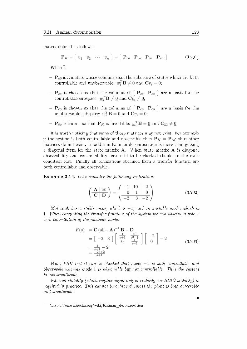
3.11. Kalman decomposition 123
matrix dened as follows:
PK =[v1 v2 · · · vn
]=[
Pco Pco Pco Pco
](3.201)
Where7:
− Pco is a matrix whose columns span the subspace of states which are bothcontrollable and unobservable: wTi B 6= 0 and Cvi = 0;
− Pco is chosen so that the columns of[
Pco Pco
]are a basis for the
controllable subspace: wTi B 6= 0 and Cvi 6= 0;
− Pco is chosen so that the columns of[
Pco Pco
]are a basis for the
unobservable subspace: wTi B = 0 and Cvi = 0;
− Pco is chosen so that PK is invertible: wTi B = 0 and Cvi 6= 0.
It is worth noticing that some of those matrices may not exist. For exampleif the system is both controllable and observable then PK = Pco; thus othermatrices do not exist. In addition Kalman decomposition is more than gettinga diagonal form for the state matrix A. When state matrix A is diagonalobservability and controllability have still to be checked thanks to the rankcondition test. Finally all realizations obtained from a transfer function areboth controllable and observable.
Example 3.14. Let's consider the following realization:
(A B
C D
)=
−1 10 −20 1 0
−2 3 −2
(3.202)
Matrix A has a stable mode, which is −1, and an unstable mode, which is1. When computing the transfer function of the system we can observe a pole /zero cancellation of the unstable mode:
F (s) = C (sI−A)−1 B + D
=[−2 3
] [ 1s+1
10s2−1
0 1s−1
] [−20
]− 2
= 4s+1 − 2
= −2s+2s+1
(3.203)
From PBH test it can be checked that mode −1 is both controllable andobservable whereas mode 1 is observable but not controllable. Thus the systemis not stabilizable.
Internal stability (which implies input-output stability, or BIBO stability) isrequired in practice. This cannot be achieved unless the plant is both detectableand stabilizable.
7https://en.wikipedia.org/wiki/Kalman_decomposition

124 Chapter 3. Analysis of Linear Time Invariant systems
3.12 Minimal realization (again!)
We have seen that a realization of a transfer function F(s) is minimal if thereexists no realization of lesser order whose transfer function is F(s). The orderof a realization is the size of matrix A.
A realization is said to be minimal if and only if the realization is bothcontrollable and observable. Consequently a minimal realization of the transferfunction F(s) = C (sI−A)−1 B + D is Cco (sI−Aco)
−1 Bco + D:
F(s) =
(A B
C D
)=
(Aco Bco
Cco D
)(3.204)
Indeed:
(sI−A)−1 B =
sI−Aco −A12 −A13 −A14
0 sI−Aco 0 −A24
0 0 sI−Aco −A34
0 0 0 sI−Aco
−1
Bco
Bco
00
=
(sI−Aco)
−1 ∗ ∗ ∗0 (sI−Aco)
−1 ∗ ∗0 0 (sI−Aco)
−1 ∗0 0 0 (sI−Aco)
−1
Bco
Bco
00
=
∗
(sI−Aco)−1 Bco
00
(3.205)
And:
F(s) = C (sI−A)−1 B + D
=[
0 Cco 0 Cco
] ∗
(sI−Aco)−1 Bco
00
+ D
= Cco (sI−Aco)−1 Bco + D
=
(Aco Bco
Cco D
)(3.206)
The number of states of a minimal realization can be evaluated by the rankof the product of the observability and the controllability matrix 8.
8Albertos P., Sala A., Multivariable Control Systems, Springer, p78

Chapter 4
Observer design
4.1 Introduction
The components of the state vector x may not be fully available asmeasurements. Observers are used in order to estimate state variables of adynamical system, which will be denoted x in the following, from the outputsignal y(t) and the input signal u(t) as depicted on Figure 4.1.
Several methods may be envisioned to reconstruct the state vector x(t) of asystem from the observation of its output signal y(t) and the knowledge of theinput signal u(t):
− From the output equation y(t) = Cx(t) + Du(t) we can imagine to build
x(t) from the relationship x(t) = C−1(y(t)−Du(t)
). Unfortunately this
relationship holds as soon as matrix C is square and invertible, which isseldom the case;
− Assuming that the size of the state vector is n we may also imagine to takethe derivative of the output signal n− 1 times and use the state equationx(t) = Ax(t) + Bu(t) to get n equations where the state vector x(t) isthe unknown. Unfortunately this not possible in practice because eachderivative of an unsmoothed signal increases its noise ;
Figure 4.1: Observer principle

126 Chapter 4. Observer design
− We can also use a Luenberger observer which will be developed in thenext section. David Gilbert Luenberger, born in 1937 in Los Angeles, isan American mathematical scientist1. The theory of full order observeroriginated in the work of Luenberger in 1964.
This chapter focuses on observers design. More specically Luenbergerobserver, state observer for SISO systems in observable canonical form, stateobserver for SISO systems in arbitrary state-space representation and stateobserver for MIMO systems will be presented. We will also presentreduced-order observer design.
4.2 Luenberger observer
Consider the following state space representation where x(t) denotes the statevector, y(t) the measured output and u(t) the control input:
x(t) = Ax(t) + Bu(t)y(t) = Cx(t) + Du(t)
(4.1)
We assume that state vector x(t) cannot be measured. The goal of theobserver is to estimate x(t) based on the observation y(t). Luenberger observerprovides an estimation x(t) of the state vector x(t) through the followingdierential equation where output signal y(t) and input signal u(t) are knownand where matrices F , J and L have to be determined:
˙x(t) = Fx(t) + Ju(t) + Ly(t) (4.2)
The estimation error e(t) is dened as follows:
e(t) = x(t)− x(t) (4.3)
The time derivative of the estimation error reads:
e(t) = x(t)− ˙x(t)= Ax(t) + Bu(t)− Fx(t)− Ju(t)− Ly(t)
(4.4)
Thanks to the output equation y(t) = Cx(t) + Du(t) and the relationshipx(t) = e(t) + x(t) we get:
e(t) = Ax(t) + Bu(t)− Fx(t)− Ju(t)− L (Cx(t) + Du(t))= (A− LC)x(t) + (B− J− LD)u(t)− Fx(t)= (A− LC) e(t) + (B− J− LD)u(t) + (A− LC− F) x(t)
(4.5)
As soon as the purpose of the observer is to move the estimation error e(t)towards zero independently of control u(t) and true state vector x(t) we choosematrices J and F as follows:
J = B− LDF = A− LC
(4.6)
1https://en.wikipedia.org/wiki/David_Luenberger

4.2. Luenberger observer 127
Thus the dynamics of the estimation error e(t) reduces to be:
e(t) = (A− LC) e(t) (4.7)
In order that the estimation error e(t) moves towards zero, meaning that theestimated state vector x becomes equal to the actual state vector x(t), matrixL shall be chosen such that all the eigenvalues of A − LC are situated in theleft half plane.
With the expression of matrices J and F the dynamics of the Luenbergerobserver can be written as follows:
˙x(t) = Fx(t) + Ju(t) + Ly(t)
= (A− LC) x(t) + (B− LD)u(t) + Ly(t)(4.8)
That is:˙x(t) = Ax(t) + Bu(t) + L
(y(t)− y(t)
)(4.9)
Where:y(t) = Cx(t) + Du(t) (4.10)
Thus the dynamics of the Luenberger observer is the same than the dynamicsof the original system with the additional term L
(y(t)− y(t)
)where L is a gain
to be set. This additional term is proportional to the error y(t) − y(t). Itenables to drive the estimated state x(t) towards its actual value x(t) when themeasured output y(t) deviates from the estimated output y(t).
In order to compute a state space representation and the transfer functionof the observer we rst identify its input and output.
− As discussed previously the input vector uo(t) of the observer is composedof the output y(t) of the plant whose state is estimated and its input u(t):
uo(t) =
[y(t)
u(t)
](4.11)
− The output yo(t) of the observer is the estimated state vector x(t) of the
plant:yo(t) = x(t) (4.12)
Consequently (4.9) and (4.10) can be organized to obtain a state spacerepresentation of the observer:
˙x(t) = Ax(t) + Bu(t) + L(y(t)− y(t)
)= Ax(t) + Bu(t) + L
(y(t)−Cx(t)−Du(t)
)= (A− LC) x(t) +
[L B− LD
] [ y(t)
u(t)
]= (A− LC) x(t) +
[L B− LD
]uo(t)
:= Aobsx(t) + Bobsuo(t)yo(t) = x(t)
= Ix(t) + 0uo(t):= Cobsx(t) + Dobsuo(t)
(4.13)

128 Chapter 4. Observer design
Figure 4.2: Block diagram of the state-space representation of an observer
Finally the transfer function of the observer, which is obviously a Multi-Input Multi-Output (MIMO) system, reads:
Gobs(s) = Cobs (sI−Aobs)−1 Bobs + Dobs
= (sI− (A− LC))−1 [ L B− LD] (4.14)
The block diagram corresponding to state-space representation (4.9) isshown in Figure 4.2.
In the following we will assume that the system is observable, or at leastdetectable, such that it is possible to design a state observer.
4.3 State observer for SISO systems in observablecanonical form
Let
(A B
C D
)be an observable Single-Input Single-Output (SISO) linear time-
invariant system of order n and let χA−LC(s) be an imposed nth order monicpolynomial (a monic polynomial is a polynomial in which the leading coecient,that is the nonzero coecient of highest degree, is equal to 1). PolynomialχA−LC(s) corresponds to the characteristic polynomial of matrix A − LC. Itis formed thanks to the predened eigenvalues λL1, · · · , λLn assigned for thedynamics of the observer:
χA−LC(s) = det (sI− (A− LC)) = (s− λL1) · · · (s− λLn) (4.15)
When expanding the preceding product we get:
χA−LC(s) = sn + pn−1sn−1 + · · ·+ p1s+ p0 (4.16)
We begin with the case where the system realization
(A B
C D
)is the

4.3. State observer for SISO systems in observable canonical form 129
observable canonical form. Then matrices Ao and Co are the following:
Ao =
0 0 0 −a0
1 0 0. . . −a1
0 1 0. . . −a2
.... . .
. . ....
0 0 1 −an−1
Co =
[0 0 · · · 0 1
](4.17)
Matrices Bo and D will not be used.Let Lo be the observer gain matrix when the observable canonical form of
the system is used. For a SISO system this is a n × 1 matrix. Let Li be the(scalar) component in the ith row of matrix Lo:
Lo =
L1...Ln
(4.18)
Then matrix Ao − LoCo reads:
Ao − LoCo =
0 0 0 −a0
1 0 0. . . −a1
0 1 0. . . −a2
.... . .
. . ....
0 0 1 −an−1
−
L1...Ln
[ 0 0 · · · 0 1]
=
0 0 0 −a0 − L1
1 0 0. . . −a1 − L2
0 1 0. . . −a2 − L3
.... . .
. . ....
0 0 1 −an−1 − Ln
(4.19)
Since this matrix still remains in the observable canonical form itscharacteristic polynomial is readily written as follows:
χA−LC(s) = det (A− LC)= det (Ao − LoCo)= sn + (an−1 + Ln) sn−1 + · · ·+ (a1 + L2) s+ a0 + L1
(4.20)
Identifying Equations (4.16) and (4.20) leads to the expression of eachcomponent of the observer matrix Lo:
p0 = a0 + L1
p1 = a1 + L2...pn−1 = an−1 + Ln
⇔ Lo =
L1
L2...Ln
=
p0 − a0
p1 − a1...
pn−1 − an−1
(4.21)

130 Chapter 4. Observer design
4.4 State observer for SISO systems in arbitrarystate-space representation
When an arbitrary state-space representation is used the system has to beconverted into the observable canonical form via a similarity transformation.Let Po be the matrix of the similarity transformation which enables to get theobservable canonical form. We get:
x(t) = Poxo(t)⇔ xo(t) = P−1o x(t) (4.22)
We have seen in the chapter dedicated to Realization of transfer functionsthat Po is a constant nonsingular change of basis matrix which is obtainedthrough the following relationship:
Po = Q−1o Qoo (4.23)
Where:
− Qo is the observability matrix in the actual basis:
Qo =
C
CA...
CAn−1
(4.24)
− and Qoo the observability matrix expressed in the observable canonicalbasis (which is readily obtained through det (sI−A)).
Thus the state equation of the observer (4.9) reads:
˙xo(t) = Aoxo(t) + Bou(t) + Lo(y(t)− y(t)
)⇔ P−1
o˙x(t) = AoP
−1o x(t) + Bou(t) + Lo
(y(t)− y(t)
)⇔ ˙x(t) = PoAoP
−1o x(t) + PoBou(t) + PoLo
(y(t)− y(t)
) (4.25)
That is:˙x(t) = Ax(t) + Bu(t) + L
(y(t)− y(t)
)(4.26)
Where:
L = PoLo (4.27)
And: A = PoAoP
−1o
B = PoBo(4.28)
Example 4.1. Design an observer for the following plant:x(t) =
[−1 00 −2
]x(t) +
[12
]u(t)
y(t) =[
3 5]x(t)
(4.29)

4.4. State observer for SISO systems in arbitrary state-space representation131
As far as this is a modal (or diagonal) state space representation, plant'sobservability is readily checked by inspecting row of output matrix C: becausethere is no null element in the output matrix C we conclude that the plant isobservable by applying Gilbert's criteria.
The poles of the observer shall be chosen faster than the dynamics of theplant, whose modes are −1 and −2. We choose (for example) to locate the polesof the observer at λL1 = −10 and λL2 = −20.
We will rst design the observer assuming that we have the observablecanonical form of the SISO system. The observable canonical form is readilyobtained through det(sI−A):
det(sI−A) = (s+ 1)(s+ 2) = s2 + 3 s+ 2 := s2 + a1 s+ a0
⇒ Ao =
[0 −21 −3
]and Co =
[0 1
] (4.30)
On the other hand the characteristic polynomial of the observer is formedthanks to the predened eigenvalues assigned for the dynamics of the observer:
χA−LC(s) = (s− λL1) (s− λL2) = (s+ 10) (s+ 20)= s2 + 30 s+ 200 := s2 + p1 s+ p0
(4.31)
Applying relationship (4.21) we get:
Lo =
[L1
L2
]=
[p0 − a0
p1 − a1
]=
[200− 230− 3
]=
[19827
](4.32)
Now let's compute the similarity transformation matrix Po which enables toget the observable canonical form.
Po = Q−1o Qoo (4.33)
Where:
− Qo is the observability matrix in the actual basis:
Qo =
[C
CA
]=
3 5[3 5
] [−1 00 −2
] =
[3 5−3 −10
](4.34)
− and Qoo the observability matrix expressed in the observable canonical basis(which is readily obtained through det (sI−A)):
Qoo =
[Co
CoAo
]=
0 1[0 1
] [0 −21 −3
] =
[0 11 −3
](4.35)
Thus:
Po = Q−1o Qoo =
[3 5−3 −10
]−1 [0 11 −3
]= −1
15
[−10 −5
3 3
] [0 11 −3
]= −1
15
[−5 53 −6
]= 1
15
[5 −5−3 6
] (4.36)

132 Chapter 4. Observer design
We nally get:
L = PoLo =1
15
[5 −5−3 6
] [19827
]=
[57−28.8
](4.37)
4.5 Ackermann's formula
Ackermann's formula states that the observer gain matrix L of a SISO systemin arbitrary state-space representation can be obtained as the product betweenthe assigned characteristic polynomial χA−LC(s) of matrix A − LC evaluatedat matrix A and vector q
o:
L = χA−LC(A)qo
(4.38)
To get this result we rst recall that similarity transformation generatesequivalent state-space representations. Let Po be the matrix of the similaritytransformation which enables to get the observable canonical form. Starting
from a state-space representations
(A B
C D
)in an arbitrary basis, the
observable canonical form is obtained through the following relationships:Ao = P−1
o APo
Bo = P−1o B
Co = CPo
(4.39)
Consequently matrix Ao − LoCo reads:
Ao − LoCo = P−1o APo − LoCPo
= P−1o (A−PoLoC) Po
(4.40)
This equation indicates that the observer gain matrix L in arbitrary state-space representation reads:
L = PoLo (4.41)
We have seen in the chapter dedicated to Realization of transfer functionsthat Po is a constant nonsingular change of basis matrix which is obtainedthrough the state matrix A and vector q
o:
Po =[qo
Aqo· · · An−1q
o
](4.42)
Vector qois the last column of the inverse of the observability matrix Qo:
Q−1o =
[∗ · · · ∗ q
o
]where Qo =
C
CA...
CAn−1
(4.43)

4.5. Ackermann's formula 133
Then we recall CayleyHamilton theorem. Let χAo(s) be the characteristicpolynomial of the n × n matrix Ao. We write the characteristic polynomialχAo(s) of matrix Ao as follows:
χAo(s) := det(sI−Ao) = sn + an−1sn−1 + · · ·+ a1s+ a0 (4.44)
The CayleyHamilton theorem states that substituting matrix Ao for s inthe characteristic polynomial χAo(s) of matrix Ao results in the zero matrix 2:
χAo(Ao) = 0 = Ano + an−1A
n−1o + · · ·+ a1Ao + a0I (4.45)
Let χA−LC(s) be the characteristic polynomial of matrix Ao − LoCo. Wehave seen that when predened eigenvalues λL1, · · · , λLn are assigned for thedynamics of the observer the characteristic polynomial of matrix Ao − LoCo
reads:χA−LC(s) = det (sI− (Ao − LoCo))
= (s− λL1) · · · (s− λLn)= sn + pn−1s
n−1 + · · ·+ p1s+ p0
(4.46)
Substituting s for matrix Ao leads to the following relationship:
χA−LC(Ao) = Ano + pn−1A
n−1o + · · ·+ p1Ao + p0I (4.47)
Note that χA−LC(Ao) is not equal to 0 because χA−LC(s) is not thecharacteristic polynomial of matrix Ao.
Thanks to Equation (4.21) and the relationship pi = ai + Li we get:
χA−LC(Ao) = Ano + (an−1 + Ln−1) An−1
o + · · ·+ (a1 + L1) Ao + (a0 + L0) I (4.48)
By subtracting Equations (4.45) to (4.48) we get:
χA−LC(Ao) = Ln−1An−1o + · · ·+ L1Ao + L0I (4.49)
Let u be the vector dened by:
u =
10...0
(4.50)
Due to the special form of matrix Ao we have:
Aou =
010...
, A2ou =
0010...
, · · · , An−1o u =
0...01
(4.51)
2https://en.wikipedia.org/wiki/CayleyHamilton_theorem

134 Chapter 4. Observer design
Thus multiplying Equation (4.49) by u leads to the following relationship:
χA−LC(Ao)u =
L0
L1...
Ln−1
= Lo (4.52)
Thus we get the expression of the observer matrix Lo when we use theobservable canonical form.
We multiply Equation (4.52) by Po and use the fact that
Ako =
(P−1o APo
)k= P−1
o AkPo to get the expression of the observer gainmatrix L in arbitrary state space representation:
L = PoLo= PoχA−LC(Ao)u= χA−LC(PoAo)u= χA−LC(PoAoP
−1o Po)u
= χA−LC(PoAoP−1o )Pou
= χA−LC(A)Pou
(4.53)
Because u is the vector dened by u =
10...0
we get using (4.42):
Pou = qo
(4.54)
Consequently Equation (4.53) reduces to be the Ackermann's formula (4.38):
L = χA−LC(A)qo
(4.55)
4.6 State observer for MIMO systems -Roppenecker's formula
We have seen in Equation (4.7) that the dynamics of the estimation error e(t)reads:
e(t) = (A− LC) e(t) (4.56)
The purpose of this section is to design the observer gain matrix L suchthat the eigenvalues of matrix A − LC are assigned to predened eigenvaluesλL1, · · · , λLn where n is the size of matrix A.
Let λK1, · · · , λKn be n distinct specied eigenvalues of the closed loop statematrix A − LC. Furthermore we assume that eigenvalues of matrix A do notshift (meaning that they are dierent) the eigenvalues of the closed loop statematrix A− LC. Then it can be shown that the transpose of the observer gainmatrix L can be computed as follows where p
idenotes parameter vectors:
LT = −[p
1· · · p
n
] [wL1 · · · wLn
]−1(4.57)

4.6. State observer for MIMO systems - Roppenecker's formula 135
Where vector wLi is related to parameter vector pithrough the following
relationship: [AT − λLiI CT
] [ wLipi
]= 0 (4.58)
This is the so-called Roppenecker's formula to get the observer gain matrixL.
To get this result we rewrite the dynamics of the estimation error e(t) asfollows:
eT (t) = (A− LC)T eT (t)⇔ eT (t) =(AT −CTLT
)eT (t) (4.59)
Let wLi be an eigenvector of matrix (A− LC)T . As far as (A− LC)T and(A− LC) have the same eigenvalues, which are the predened eigenvalues λLi,we can write: (
AT −CTLT)wLi = λLiwLi (4.60)
The preceding equation can be written as follows:(AT − λLiI
)wLi = CTLTwLi (4.61)
That is:wLi =
(AT − λLiI
)−1CTLTwLi (4.62)
Then we introduce n parameter vectors pidened as follows;
pi
= −LTwLi (4.63)
Each parameter vector piis a p× 1 vector where p is the number of rows of
matrix C, that is the number of outputs of the system.Using parameter vector p
iEquation (4.62) reads:
wLi = −(AT − λLiI
)−1CT p
i(4.64)
Writing Equation (4.63) for the n distinct predened eigenvaluesλL1, · · · , λLn leads to the following relationship:[
p1· · · p
n
]= −LT
[wL1 · · · wLn
](4.65)
Finally the transpose of the observer gain matrix L can be computed asfollows:
LT = −[p
1· · · p
n
] [wL1 · · · wLn
]−1(4.66)
We have retrieved the so-called Roppenecker's formula to get the observergain matrix L.
It is worth noticing the following facts:
− Using equation (4.63) within Equation (4.61) it is clear that parametervectors p
ishall satisfy the following relationship:(
AT − λLiI)wLi = −CT p
i(4.67)

136 Chapter 4. Observer design
That is: [AT − λLiI CT
] [ wLipi
]= 0 (4.68)
It is clear from the previous equation that each (n+ p) × 1 vector[wLipi
]belong to the null-space of matrix
[AT − λLiI CT
]. So once
any (n+ p) × 1 vector which belongs to the null-space of matrix[AT − λLiI CT
]has been found, its p bottom rows are used to form
vector parameter pi. In the MIMO case several possibilities are oered.
− By taking the transpose of equation (4.68) we get the following expression:
[wTLi pT
i
] [ A− λLiIC
]= 0 (4.69)
We recognize in matrix
[A− λLiI
C
]the key matrix used in the PBH
observability test;
− If we wish to keep an eigenvalue λi of matrix A within the set of eigenvaluesof A−LC then Equation (4.61) is equal to zero because in that case wLiis also an eigenvector of A:
λLi = λi ⇒(AT − λLiI
)wLi = −CT p
i=(AT − λiI
)wLi = 0 (4.70)
Consequently we have to replace piby 0 and wLi by eigenvector wi of A
corresponding to λi in the Roppenecker's formula (4.57);
− If we chose a complex eigenvalue λLi then its complex conjugate must alsobe chosen. Let's λLiR and λLiI be the real part and the imaginary partof λLi, wLiR and wLiI be the real part and the imaginary part of wLi andpiR
and piIbe the real part and the imaginary part of p
irespectively:
λLi = λLiR + jλLiIwLi = wLiR + jwLiIpi
= piR
+ jpiI
(4.71)
Then equation (4.68) reads:(AT − (λLiR + jλLiI) I
)(wLiR + jwLiI) + CT
(piR
+ jpiI
)= 0 (4.72)
Taking the complex conjugate of the preceding equation reads:(AT − (λLiR − jλLiI) I
)(wLiR − jwLiI) + CT
(piR− jp
iI
)= 0 (4.73)
Summing and subtracting Equations (4.72) and (4.73) reads: (AT − λLiRI
)wLiR + λLiIwLiI + CT p
iR= 0(
AT − λLiRI)wLiI − λLiIwLiR + CT p
iI= 0
(4.74)

4.6. State observer for MIMO systems - Roppenecker's formula 137
That is in vector form:
[AT − λLiRI λLiII CT 0−λLiII AT − λLiRI 0 CT
]wLiRwLiIpiRpiI
= 0 (4.75)
In Equation (4.57) vectors pi, p∗
i(where ∗ denotes complex conjugate),
wLi and w∗Li are replaced by vectors p
iR, p
iI, wLiR and wLiI , respectively.
− In the SISO case the observer gain matrix L no more depends on parametervectors p
i. Indeed is that case the observer gain matrix L is obtained as
follows:
LT =[
1 · · · 1][ (
AT − λL1I)−1
CT · · ·(AT − λLnI
)−1CT
]−1(4.76)
To get this result we start by observing that in the SISO case parametervector are scalars; they will be denoted pi. Let vector li be dened asfollows:
li = −(AT − λLiI
)−1CT (4.77)
Then Equation (4.57) reads:
LT = −[p1 · · · pn
] [l1p1 · · · lnpn
]−1(4.78)
Let's rearrange the term[l1p1 · · · lnpn
]−1as follows:
[l1p1 · · · lnpn
]−1=
[ l1 · · · ln] p1 0
. . .
0 pn
−1
=
p1 0. . .
0 pn
−1 [
l1 · · · ln]−1
=
∏i6=1 pi∏ni=1 pi
0
. . .
0∏i 6=n pi∏ni=1 pi
[ l1 · · · ln]−1
(4.79)
Multiplying this expression by −[p1 · · · pn
]leads to the expression
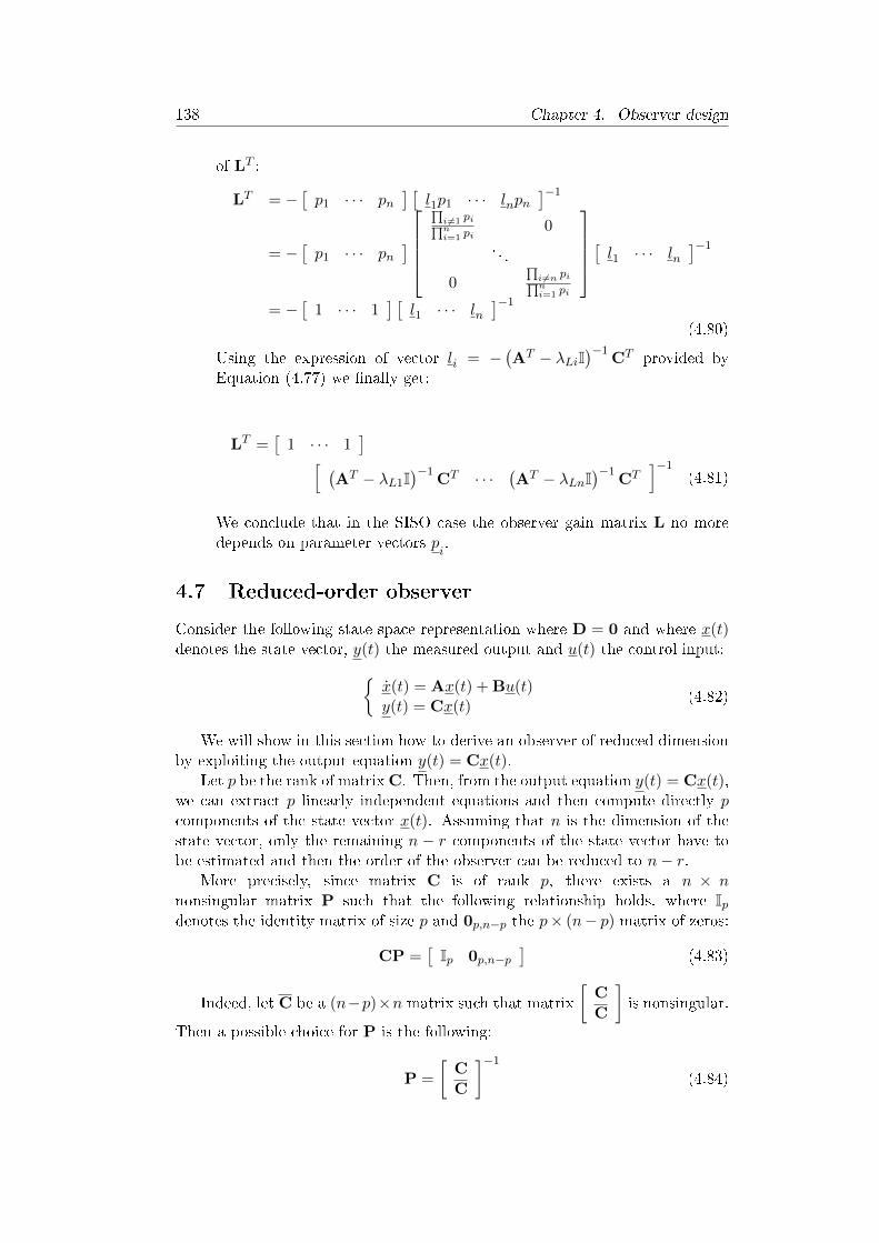
138 Chapter 4. Observer design
of LT :
LT = −[p1 · · · pn
] [l1p1 · · · lnpn
]−1
= −[p1 · · · pn
]
∏i6=1 pi∏ni=1 pi
0
. . .
0∏i 6=n pi∏ni=1 pi
[ l1 · · · ln]−1
= −[
1 · · · 1] [
l1 · · · ln]−1
(4.80)
Using the expression of vector li = −(AT − λLiI
)−1CT provided by
Equation (4.77) we nally get:
LT =[
1 · · · 1][ (
AT − λL1I)−1
CT · · ·(AT − λLnI
)−1CT
]−1(4.81)
We conclude that in the SISO case the observer gain matrix L no moredepends on parameter vectors p
i.
4.7 Reduced-order observer
Consider the following state space representation where D = 0 and where x(t)denotes the state vector, y(t) the measured output and u(t) the control input:
x(t) = Ax(t) + Bu(t)y(t) = Cx(t)
(4.82)
We will show in this section how to derive an observer of reduced dimensionby exploiting the output equation y(t) = Cx(t).
Let p be the rank of matrix C. Then, from the output equation y(t) = Cx(t),we can extract p linearly independent equations and then compute directly pcomponents of the state vector x(t). Assuming that n is the dimension of thestate vector, only the remaining n − r components of the state vector have tobe estimated and then the order of the observer can be reduced to n− r.
More precisely, since matrix C is of rank p, there exists a n × nnonsingular matrix P such that the following relationship holds, where Ipdenotes the identity matrix of size p and 0p,n−p the p× (n− p) matrix of zeros:
CP =[Ip 0p,n−p
](4.83)
Indeed, let C be a (n−p)×n matrix such that matrix
[C
C
]is nonsingular.
Then a possible choice for P is the following:
P =
[C
C
]−1
(4.84)

4.7. Reduced-order observer 139
Hence, using (4.83), we can write:
y(t) = Cx(t) = CPP−1x(t) =[Ip 0p,n−p
]x∗(t) (4.85)
where:
x∗(t) = P−1x(t)⇔ x(t) = Px∗(t) (4.86)
Hence, mapping the system in the new state vector x∗(t) via the similaritytransformation P, we obtain the following state space representation:
x∗(t) = P−1APx∗(t) + P−1Bu(t)y(t) = CPx∗(t)
(4.87)
From the fact that CP =[Ip 0p,n−p
], it can be seen that the rst p
components of the new state vector x∗(t) are equal to y(t). Thus we can write:
CP =[Ip 0p,n−p
]⇒ x∗(t) =
[y(t)
xr(t)
](4.88)
As far as the p rst components of the new state vector x∗(t) are equalto y(t), they are available through measurements and thus there is no need toestimate those components. Consequently the reduced-order observer focuseson the estimation of the remaining state vector xr(t).
The state equation (4.87) can be written as follows:x∗(t) :=
[y(t)
xr(t)
]=
[A∗11 A∗12
A∗21 A∗22
] [y(t)
xr(t)
]+
[B∗1B∗2
]u(t)
y(t) =[Ip 0p,n−p
] [ y(t)
xr(t)
]:= C∗x∗(t)
(4.89)
Let's split matrix P as follows, where P1 is a n×pmatrix and P2 a n×(n−p)matrix:
P =
[C
C
]−1
:=[
P1 P2
](4.90)
Then we get:[
A∗11 A∗12
A∗21 A∗22
]= P−1AP =
[CAP1 CAP2
CAP1 CAP2
][
B∗1B∗2
]= P−1B =
[CB
CB
] (4.91)
To design an observer for xr(t), we use the knowledge that an observer hasthe same structure as the system plus the driving feedback term whose role is toreduce the estimation error to zero3. Hence, an observer for xr(t) reads:
˙xr(t) = A∗21y(t) + A∗22xr(t) + B∗2u(t) + Lr(y(t)− y(t)
)(4.92)
3Zoran Gajic, Introduction to Linear and Nonlinear Observers, Rutgers University,https://www.ece.rutgers.edu/gajic/

140 Chapter 4. Observer design
Unfortunately, since y(t) = y(t), the dierence y(t)− y(t) does not carry anyinformation about xr(t). Nevertheless, by taking the time derivative of y(t), weget the rst equation of (4.89) which carries information about xr(t):
y(t) = A∗11y(t) + A∗12xr(t) + B∗1u(t)
⇒ A∗12xr(t) = y(t)−A∗11y(t)−B∗1u(t)(4.93)
Regarding yr(t) := A∗12xr(t) as a virtual output of the reduced state
equation, the observer for xr(t) nally reads:˙xr(t) = A∗21y(t) + A∗22xr(t) + B∗2u(t) + Lr
(yr(t)−A∗12xr(t)
)yr(t) = y(t)−A∗11y(t)−B∗1u(t)
(4.94)
Furthermore the dynamics of the error er(t) = xr(t)− xr(t) reads as follows:
er(t) = xr(t)− xr(t)⇒ er(t) = xr(t)− ˙xr(t)
= A∗21y(t) + A∗22xr(t) + B∗2u(t)
−(A∗21y(t) + A∗22xr(t) + B∗2u(t) + Lr
(yr(t)−A∗12xr(t)
))= (A∗22 − LrA
∗12) er(t)
(4.95)Consequently, designing the observer gain Lr such that the characteristic
polynomial of matrix A∗22 − LrA∗12 is Hurwitz leads to the asymptotic
convergence of the estimates xr(t) towards xr(t). Such a design is alwayspossible as soon as the pair (A∗22,A
∗12) is observable, which is a consequence of
the observability of the pair (A,C) (this can be shown using PBH test3).Since it is not wise to use y(t) because in practice the dierentiation process
introduces noise, we will estimate vector xry(t) rather than xr(t). Vector xry(t)is dened as follows:
xry(t) := xr(t)− Lry(t) (4.96)
From (4.94), we get the following observer for xry(t):
˙xry(t) = ˙xr(t)− Lry(t)
= A∗21y(t) + A∗22xr(t) + B∗2u(t) + Lr
(yr(t)−A∗12xr(t)
)− Lry(t)
= A∗21y(t) + A∗22
(xry(t) + Lry(t)
)+ B∗2u(t)
+Lr(−A∗11y(t)−B∗1u(t)−A∗12
(xry(t) + Lry(t)
)):= Ayy(t) + Aryxry(t) + Buu(t)
(4.97)where:
Ay = A∗21 + A∗22Lr − LrA∗11 − LrA
∗12Lr
Ary = A∗22 − LrA∗12
Bu = B∗2 − LrB∗1
(4.98)
Assembling the previous results, the estimation of state vector x(t) nallyreads as follows where the dynamics of xry(t) is given by (4.97):
x(t) = Px∗(t) = P
[y(t)
xr(t)
]= P
[y(t)
xry(t) + Lry(t)
](4.99)

Chapter 5
Controller design
5.1 Introduction
Controller enables to obtain stable systems which meet performancesspecications. In the case where the full state vector x(t) is available thencontroller design involves state feedback. In the more usual case where onlysome components of the state vector are available through the output vectory(t) then controller design involves output feedback in association with a stateobserver.
This chapter focuses on controllers design. More specically state feedbackcontroller for SISO systems in controllable canonical form, state feedbackcontroller for SISO systems in arbitrary state-space representation, static statefeedback controller and static output feedback controller for MIMO systemswill be presented. We will also present controller with integral action.
5.2 Static state feedback controller
Consider the following state equation where x(t) denotes the state vector andu(t) the control input:
x(t) = Ax(t) + Bu(t) (5.1)
We will assume in the following that the full state vector x(t) is availablefor control.
Let r(t) be a reference input signal. A static state feedback (or full state)controller computes the control input u(t) as a function of a state-feedback gainK and a feedforward gain matrix H as follows:
u(t) = Hr(t)−Kx(t) (5.2)
Substituting the control law (5.2) into the state equation (5.1) of the systemyields:
x(t) = (A−BK)x(t) + BHr(t) (5.3)
− The purpose of the controller gain K is at least to assign the eigenvalues ofthe closed-loop state matrix A−BK at predened locations. For MIMO

142 Chapter 5. Controller design
systems there are additional degrees of freedom which may be used forothers purposes like eigenstructure assignment;
− The purpose of the feedforward gain matrix H is to pick up the desirednal value such that the closed-loop system has no steady state error toany constant value of the reference input r(t).
In steady state conditions we have x(t) = 0 and consequently (5.3) reads:
x(t) = 0⇒ x(t) = − (A−BK)−1 BHr(t) (5.4)
On the other hand, using (5.2) the output equation y(t) = Cx(t) + Du(t)reads:
y(t) = Cx(t) + Du(t)
u(t) = −Kx(t) + Hr(t)⇒ y(t) = (C−DK)x(t) + DHr(t) (5.5)
Inserting (5.4) into (5.5) yields:
y(t) = − (C−DK) (A−BK)−1 BHr(t) + DHr(t)
=(D− (C−DK) (A−BK)−1 B
)Hr(t)
(5.6)
Then matrix H is computed such that the closed-loop system has no steadystate error to any constant value of the reference input r(t). So imposingy(t) = r(t) leads to the following expression of the feedforward gain matrixH:
y(t) = r(t)⇒ H =(D− (C−DK) (A−BK)−1 B
)−1(5.7)
In the usual case where matrix D is null the preceding relationshipsimplies as follows:
H = −(C (A−BK)−1 B
)−1(5.8)
We will see in section 5.7 that adding an integral action within the controlleris an alternative method which avoid the computation of feedforward gain matrixH.
In the following we will assume that the system is controllable, or at leaststabilizable, such that it is possible to design a state feedback controller. IndeedWonham1 has shown that controllability of an open-loop system is equivalentto the possibility of assigning an arbitrary set of poles to the transfer matrixof the closed-loop system, formed by means of suitable linear feedback of thestate.
1Wonham W., On pole assignment in multi-input controllable linear systems, IEEETransactions on Automatic Control, vol. 12, no. 6, pp. 660-665, December 1967. doi:10.1109/TAC.1967.1098739

5.3. Control of SISO systems 143
5.3 Control of SISO systems
5.3.1 State feedback controller in controllable canonical form
Let
(A B
C D
)be an controllable Single-Input Single-Output (SISO) linear
time-invariant system of order n and let χA−BK(s) be an imposed nth ordermonic polynomial (a monic polynomial is a polynomial in which the leadingcoecient, that is the nonzero coecient of highest degree, is equal to 1).Polynomial χA−BK(s) corresponds to the characteristic polynomial of matrixA − BK. It is formed thanks to the predened eigenvalues λK1 , · · · , λKnassigned for the dynamics of the controller:
χA−BK(s) = det (sI− (A−BK)) = (s− λK1) · · · (s− λKn) (5.9)
When expanding the preceding product we get:
χA−BK(s) = sn + pn−1sn−1 + · · ·+ p1s+ p0 (5.10)
We begin with the case where the system realization
(A B
C D
)is the
controllable canonical form. Then matrices Ac and Bc are the following:
Ac =
0 1 0 0
0 0 1. . . 0
. . .. . . 0
0 0 0 1−a0 −a1 −a2 · · · −an−1
Bc =
00...01
(5.11)
Matrices Cc and D will not be used.
Let Kc be the controller gain matrix when the controllable canonical formof the system is used. For a SISO system this is a 1× n matrix. Let Ki be the(scalar) component in the ith row of matrix Kc:
Kc =[K1 · · · Kn
](5.12)
Using the duality principle we can infer that the expression of the statefeedback controller for SISO systems in controllable canonical form has thefollowing expression:
Kc = LTo =[p0 − a0 · · · pn−1 − an−1
](5.13)

144 Chapter 5. Controller design
To check it just notice that when the controllable canonical form of thesystem is used then matrix Ac −BcKc reads:
Ac −BcKc =
0 1 0 0
0 0 1. . . 0
. . .. . . 0
0 0 0 1−a0 −a1 −a2 · · · −an−1
−
00...01
[K1 · · · Kn
]
=
0 1 0 0
0 0 1. . . 0
. . .. . . 0
0 0 0 1−a0 −K1 −a1 −K2 −a2 −K3 · · · −an−1 −Kn
(5.14)
Since this matrix still remains in the controllable canonical form itscharacteristic polynomial is readily written as follows:
χA−BK(s) = det (A−BK)= det (Ac −BcKc)= sn + (an−1 +Kn) sn−1 + · · ·+ (a1 +K2) s+ a0 +K1
(5.15)
Identifying Equations (5.10) and (5.15) leads to the expression of eachcomponent of the controller matrix Kc:
p0 = a0 +K1
p1 = a1 +K2...pn−1 = an−1 +Kn
⇔ Kc = [ K1 K2 · · · Kn ]= [ p0 − a0 p1 − a1 · · · pn−1 − an−1 ]
(5.16)
5.3.2 State feedback controller in arbitrary state-spacerepresentation
When an arbitrary state-space representation is used the system has to beconverted into the controllable canonical form via a similarity transformation.Let Pc be the matrix of the similarity transformation which enables to get thecontrollable canonical form. We get:
x(t) = Pcxc(t)⇔ xc(t) = P−1c x(t) (5.17)
We have seen in the chapter dedicated to Realization of transfer functionsthat P−1
c is a constant nonsingular change of basis matrix which is obtainedthrough the following relationship:
P−1c = QccQ
−1c (5.18)
Where:
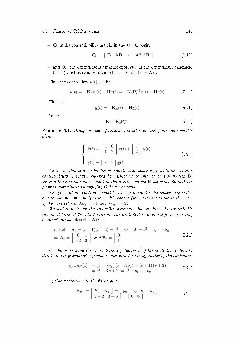
5.3. Control of SISO systems 145
− Qc is the controllability matrix in the actual basis:
Qc =[
B AB · · · An−1B]
(5.19)
− and Qcc the controllability matrix expressed in the controllable canonicalbasis (which is readily obtained through det (sI−A)).
Thus the control law u(t) reads:
u(t) = −Kcxc(t) + Hr(t) = −KcP−1c x(t) + Hr(t) (5.20)
That is:
u(t) = −Kx(t) + Hr(t) (5.21)
Where:
K = KcP−1c (5.22)
Example 5.1. Design a state feedback controller for the following unstableplant:
x(t) =
[1 00 2
]x(t) +
[12
]u(t)
y(t) =[
3 5]x(t)
(5.23)
As far as this is a modal (or diagonal) state space representation, plant'scontrollability is readily checked by inspecting column of control matrix B:because there is no null element in the control matrix B we conclude that theplant is controllable by applying Gilbert's criteria.
The poles of the controller shall be chosen to render the closed-loop stableand to satisfy some specications. We choose (for example) to locate the polesof the controller at λK1 = −1 and λK2 = −2.
We will rst design the controller assuming that we have the controllablecanonical form of the SISO system. The controllable canonical form is readilyobtained through det(sI−A):
det(sI−A) = (s− 1)(s− 2) = s2 − 3 s+ 2 := s2 + a1 s+ a0
⇒ Ac =
[0 1−2 3
]and Bc =
[01
](5.24)
On the other hand the characteristic polynomial of the controller is formedthanks to the predened eigenvalues assigned for the dynamics of the controller:
χA−BK(s) = (s− λK1) (s− λK2) = (s+ 1) (s+ 2)= s2 + 3 s+ 2 := s2 + p1 s+ p0
(5.25)
Applying relationship (5.16) we get:
Kc =[K1 K2
]=[p0 − a0 p1 − a1
]=[
2− 2 3 + 3]
=[
0 6] (5.26)

146 Chapter 5. Controller design
Now let's compute the inverse of the similarity transformation matrix P−1c
which enables to get the controllable canonical form.
P−1c = QccQ
−1c (5.27)
Where:
− Qc is the controllability matrix in the actual basis:
Qc =[
B AB]
=
[1 12 4
](5.28)
− and Qcc the controllability matrix expressed in the controllable canonicalbasis (which is readily obtained through det (sI−A)):
Qcc =[
Bc AcBc
]=
[0 11 3
](5.29)
Thus:
P−1c = QccQ
−1c =
[0 11 3
] [1 12 4
]−1
= 12
[0 11 3
] [4 −1−2 1
]= 1
2
[−2 1−2 2
] (5.30)
We nally get:
K = KcP−1c =
1
2
[0 6
] [ −2 1−2 2
]=
1
2
[−12 12
]=[−6 6
](5.31)
The feedforward gain matrix H is computed thanks to (5.7) (where D = 0):
H = −(C (A−BK)−1 B
)−1= −0.125 (5.32)
5.3.3 Ackermann's formula
Ackermann's formula states that the controller gain matrix K of a SISO systemin arbitrary state-space representation can be obtained as the product betweenvector qT
cand the assigned characteristic polynomial χA−BK(s) of matrix A−
KC evaluated at matrix A:
K = qTcχA−BK(A) (5.33)
To get this result we rst recall that similarity transformation generatesequivalent state-space representations. Let Pc be the matrix of the similaritytransformation which enables to get the controllable canonical form. Starting

5.3. Control of SISO systems 147
from a state-space representations
(A B
C D
)in an arbitrary basis, the
controllable canonical form is obtained through the following relationships:Ac = P−1
c APc
Bc = P−1c B
Cc = CPc
(5.34)
Consequently matrix Ac −BcKc reads:
Ac −BcKc = P−1c APc −P−1
c BKc
= P−1c
(A−BKcP
−1c
)Pc
(5.35)
This equation indicates that the controller gain matrix K in arbitrary state-space representation reads:
K = KcP−1c (5.36)
We have seen in the chapter dedicated to Realization of transfer functionsthat P−1
c is a constant nonsingular change of basis matrix which is obtainedthrough the state matrix A and vector qT
c:
P−1c =
qTc
qTcA...
qTcAn−1
(5.37)
Vector qTcis the last row of the inverse of the controllability matrix Qc:
Q−1c =
∗...∗qTc
where Qc =[
B AB · · · An−1B]
(5.38)
Then we recall CayleyHamilton theorem. Let χAc(s) be the characteristicpolynomial of the n × n matrix Ac. We write the characteristic polynomialχAc(s) of matrix Ac as follows:
χAc(s) := det(sI−Ac) = sn + an−1sn−1 + · · ·+ a1s+ a0 (5.39)
The CayleyHamilton theorem states that substituting matrix Ac for s inthe characteristic polynomial χAc(s) of matrix Ac results in the zero matrix2:
χAc(Ac) = 0 = Anc + an−1A
n−1c + · · ·+ a1Ac + a0I (5.40)
Let χA−BK(s) be the characteristic polynomial of matrix Ac − BcKc. Wehave seen that when predened eigenvalues λK1 , · · · , λKn are assigned for the
2https://en.wikipedia.org/wiki/CayleyHamilton_theorem

148 Chapter 5. Controller design
dynamics of the controller the characteristic polynomial of matrix Ac −BcKc
reads:χA−BK(s) = det (sI− (Ac −BcKc))
= (s− λK1) · · · (s− λKn)= sn + pn−1s
n−1 + · · ·+ p1s+ p0
(5.41)
Substituting s for matrix Ac leads to the following relationship:
χA−BK(Ac) = Anc + pn−1A
n−1c + · · ·+ p1Ac + p0I (5.42)
Note that χA−BK(Ac) is not equal to 0 because χA−BK(s) is not thecharacteristic polynomial of matrix Ac.
Thanks to Equation (5.16) and the relationship pi = ai +Ki we get:
χA−BK(Ac) = Anc + (an−1 +Kn−1) An−1
c + · · ·+ (a1 +K1) Ac + (a0 +K0) I (5.43)
By subtracting Equations (5.40) to (5.43) we get:
χA−BK(Ac) = Kn−1An−1c + · · ·+K1Ac +K0I (5.44)
Due to the fact that coecients Ki are scalar we can equivalently write:
χA−BK(Ac) = An−1c Kn−1 + · · ·+ AcK1 + IK0 (5.45)
Let uT be the vector dened by:
uT =[
1 0 · · · 0]
(5.46)
Due to the special form of matrix Ac we have:
uTAc =[
0 1 0 · · ·]
uTA2c =
[0 0 1 0 · · ·
]...uTAn−1
c =[
0 · · · 0 1] (5.47)
Thus multiplying Equation (5.45) by uT leads to the following relationship:
uTχA−BK(Ac) =[K0 K1 · · · Kn−1
]= Kc (5.48)
Thus we get the expression of the controller matrix Kc when we use thecontrollable canonical form.
We multiply Equation (5.48) by P−1c and use the fact that
Akc =
(P−1c APc
)k= P−1
c AkPc get the expression of the controller gain matrixK in arbitrary state-space representation:
K = KcP−1c
= uTχA−BK(Ac)P−1c
= uTχA−BK(AcP−1c )
= uTχA−BK(P−1c PcAcP
−1c )
= uTP−1c χA−BK(PcAcP
−1c )
= uTP−1c χA−BK(A)
(5.49)

5.4. Observer-based controller 149
Because u is the vector dened by uT =[
1 0 · · · 0]we get using (5.37):
uTP−1c = qT
c(5.50)
Consequently Equation (5.49) reduces to be the Ackermann's formula (5.33):
K = qTcχA−BK(A) (5.51)
5.3.4 Zeros of closed-loop transfer function
It is worth noticing that the zeros of the closed-loop transfer function are thesame than the zeros of the open-loop transfer function when state feedback isused. In other words, state feedback K just changes the values poles of thepoles, the zeros remaining unchanged.
To get this result, we can use the controllable canonical form to computethe closed-loop transfer function, Cc (sI−Ac + BcKc)
−1 BcH, and notice thatits numerator is independent of both state feedback gain Kc and state matrixAc. The coecients which appear in the numerator of the closed-loop transferfunction come from product CcH when the controllable canonical form is used,or CBH in general, whereas state feedback gain Kc, or K in general, onlyappears in the denominator of the closed-loop transfer function:
(sI−Ac + BcKc)−1 Bc =
1
det (sI−Ac + BcKc)
∗ ∗ 1∗ ∗ s...
......
∗ ∗ sn−1
0...01
⇒ Cc (sI−Ac + BcKc)−1 BcH =
Cc
det (sI−Ac + BcKc)
1s...
sn−1
H
(5.52)A practical use of this observation is that state feedback gain K can be used
to annihilate some zeros with negative real part (that are stable zeros).
5.4 Observer-based controller
5.4.1 Separation principle
We consider the following state-space representation of dimension n (that is thesize of state matrix A) where y(t) denotes the output vector and u(t) the inputvector:
x(t) = Ax(t) + Bu(t)y(t) = Cx(t) + Du(t)
(5.53)
When the full state x(t) cannot be measured then it is estimated thanks toan observer. This leads to an observer-based controller whose dynamics readsas follows:

150 Chapter 5. Controller design
Figure 5.1: Block diagram of the observer-based controller
˙x(t) = Ax(t) + Bu(t) + L
(y(t)− (Cx(t) + Du(t))
)u(t) = Hr(t)−Kx(t)
(5.54)
Gain matrices L, K and H are degrees of freedom which shall be set toachieve some performance criteria.
The block diagram corresponding to the observer-based controller is shownin Figure 5.1.
The estimation error e(t) is dened as follows:
e(t) = x(t)− x(t) (5.55)
The time derivative of the estimation error reads:
e(t) = x(t)− ˙x(t)= Ax(t)−Ax(t)− L
(y(t)−Cx(t)−Du(t)
)= Ax(t)−Ax(t)− L (Cx(t) + Du(t)−Cx(t)−Du(t))= Ae(t)− LCe(t)= (A− LC) e(t)
(5.56)
Combining the dynamics of the state vector x(t) and of the estimation errore(t), and using the fact that x(t) = x(t)−e(t), yields to the following state-spacerepresentation for the closed-loop system:[
x(t)e(t)
]= Acl
[x(t)e(t)
]+
[BH0
]r(t) (5.57)

5.4. Observer-based controller 151
where:
Acl =
[A−BK BK
0 A− LC
](5.58)
Gain matrices L and K shall be chosen such that the eigenvalues of matricesA − BK and A − LC are situated in the left half complex plane so that theclosed-loop system is asymptotically stable.
Furthermore it is worth noticing that matrix is block triangular.Consequently we can write:
det (sI−Acl) = det
([sI−A + BK −BK
0 sI−A + LC
])= det (sI−A + BK) det (sI−A + LC) (5.59)
In other words the eigenvalues of the closed-loop system are obtained bythe union of the eigenvalues of matrix A−BK, that is the state matrix of theclosed-loop system without the observer, and the eigenvalues of matrix A−LC,that is the state matrix of the closed-loop system without the controller. Thisresult is known as the separation principle. As a consequence the observerand the controller can be designed separately: the eigenvalues obtained thanksto the controller gain K assuming full state feedback are independent of theeigenvalues obtained thanks to the observer gain L assuming no controller.
Usually observer gain L is chosen such that the eigenvalues of matrix A−LCare around 5 to 10 times faster than the eigenvalues of matrix A−BK, so thatthe state estimation moves towards the actual state as early as possible.
Furthermore the reference input r(t) has no inuence on the dynamics ofthe estimation error e(t). Consequently the feedforward gain matrix H is stillgiven by Equation (5.7).
5.4.2 Example
Design an output feedback controller for the following unstable plant:x(t) =
[1 00 2
]x(t) +
[12
]u(t)
y(t) =[
3 5]x(t)
(5.60)
The poles of the controller shall be chosen to render the closed-loop stableand to satisfy some specications. We choose (for example) to locate the polesof the controller at λK1 = −1 and λK2 = −2.
First we check that is system is observable and controllable.
We have seen in example 5.1 how to design a state feedback controller. Byapplying the separation principle the observer which estimates the state vectorx(t) which will feed the controller can be designed separately from the controller.We have obtained:
K =[−6 6
]H = −0.125
(5.61)

152 Chapter 5. Controller design
As mentioned the eigenvalues of the observer are chosen around 5 to 10times faster than the eigenvalues achieved thanks to the controller. As far asthe closed-loop poles obtained thanks to the controller are located at λK1 = −1and λK2 = −2 we choose (for example) to locate the poles of the observer atλL1 = −10 and λL2 = −20.
As described in the chapter dedicated to Observer design, we rst designthe observer assuming that we have the observable canonical form of the SISOsystem. The observable canonical form is readily obtained through det(sI−A):
det(sI−A) = (s− 1)(s− 2) = s2 − 3 s+ 2 := s2 + a1 s+ a0
⇒ Ao =
[0 −21 3
]and Co =
[0 1
] (5.62)
On the other hand the characteristic polynomial of the observer is formedthanks to the predened eigenvalues assigned for the dynamics of the observer:
χA−LC(s) = (s− λL1) (s− λL2) = (s+ 10) (s+ 20)= s2 + 30 s+ 200 := s2 + p1 s+ p0
(5.63)
Applying relationship (4.21) we get:
Lo =
[L1
L2
]=
[p0 − a0
p1 − a1
]=
[200− 230 + 3
]=
[19833
](5.64)
Now let's compute the similarity transformation matrix Po which enablesto get the observable canonical form.
Po = Q−1o Qoo (5.65)
Where:
− Qo is the observability matrix in the actual basis:
Qo =
[C
CA
]=
3 5[3 5
] [1 00 2
] =
[3 53 10
](5.66)
− and Qoo the observability matrix expressed in the observable canonicalbasis (which is readily obtained through det (sI−A)):
Qoo =
[Co
CoAo
]=
0 1[0 1
] [0 −21 3
] =
[0 11 3
](5.67)
Thus:
Po = Q−1o Qoo =
[3 53 10
]−1 [0 11 3
]= 1
15
[10 −5−3 3
] [0 11 3
]= 1
15
[−5 −53 6
] (5.68)
We nally get:
L = PoLo =1
15
[−5 −53 6
] [19833
]=
[−7752.8
](5.69)

5.4. Observer-based controller 153
Figure 5.2: Unity feedback loop
5.4.3 Transfer function
Assuming D = 0, the transfer function of the observer-based controller can beobtained by taking the Laplace transform (assuming no initial conditions) of itsstate space representation:
˙x(t) = Ax(t) + Bu(t) + L(y(t)−Cx(t)
)u(t) = −Kx(t)
(5.70)
We get:U(s) = C(s)Y (s) (5.71)
Where:C(s) = −K (sI−A + BK + LC)−1 L (5.72)
5.4.4 Algebraic controller design
We consider the unity feedback loop shown in Figure 5.2. The realization of theplant transfer function F (s) is assumed to be the following:
xp(t) = Axp(t) + Bu(t)
y(t) = Cxp(t)(5.73)
On the other hand, the realization of the controller transfer function C(s)is assumed to be the following, where gain matrices K and L are the designparameters of the controller :
xc(t) = (A−BK− LC)xc(t) + Lε(t)u(t) = Kxc(t)
(5.74)
From Figure 5.2 we get the following relationships:ε(t) = r(t)− y(t) = r(t)−Cxp(t)
u(t) = Kxc(t)(5.75)
Thus the state space realization of the unity feedback loop reads:xp(t) = Axp(t) + BKxc(t)
xc(t) = (A−BK− LC)xc(t) + L(r(t)−Cxp(t)
)y(t) = Cxp(t)
(5.76)

154 Chapter 5. Controller design
That is:[xp(t)
xc(t)
]=
[A BK−LC A−BK− LC
] [xp(t)
xc(t)
]+
[0L
]r(t)
y(t) =[
C 0] [ xp(t)
xc(t)
] (5.77)
Then the closed-loop state matrix Acl reads:
Acl =
[A BK−LC A−BK− LC
](5.78)
The closed-loop eigenvalues are the roots of the characteristic polynomialχAcl(s) dened as follows:
χAcl(s) = det (sI−Acl) = det
([sI−A −BK
LC sI−A + BK + LC
])(5.79)
Now we will use the fact that adding one column / row to another column/ row does not change the value of the determinant. Thus adding the second
row to the rst row of
[sI−A −BK
LC sI−A + BK + LC
]leads to the following
expression of χAcl(s):
χAcl(s) = det
([sI−A + LC sI−A + LC
LC sI−A + BK + LC
])(5.80)
Now subtracting the rst column to the second column of[sI−A + LC sI−A + LC
LC sI−A + BK + LC
]leads to the following expression of
χAcl(s):
χAcl(s) = det
([sI−A + LC 0
LC sI−A + BK
])(5.81)
It is worth noticing that matrix is block triangular. Consequently we canwrite:
χAcl(s) = det (sI−Acl) = det (sI−A + LC) det (sI−A + BK) (5.82)
In other words the eigenvalues of the closed-loop system are obtained bythe union of the eigenvalues of matrix A−BK, that is the state matrix of theclosed-loop system without the observer, and the eigenvalues of matrix A−LC,that is the state matrix of the closed-loop system without the controller. Thisresult is known as the separation principle. As a consequence the observerand the controller can be designed separately: the eigenvalues obtained thanksto the controller gain K assuming full state feedback are independent of theeigenvalues obtained thanks to the observer gain L assuming no controller.
It is worth noticing that the same result is achieved when the controller C(s)is put in the feedback loop as shown in Figure 5.3.

5.5. Control of MIMO systems 155
Figure 5.3: Feedback loop with C(s)
5.5 Control of MIMO systems
5.5.1 Frequency domain approach for state feedback
We consider the state-space representation (5.83) where the state vector x is ofdimension n (that is the size of state matrix A). In addition u(t) denotes theinput vector. We will assume the following state feedback:
x(t) = Ax(t) + Bu(t)u(t) = −Kx(t) + Hr(t)
(5.83)
It can be shown that thanks to the Schur's formula the closed-loopcharacteristic polynomial det(sI−A + BK) reads as follows:
det (sI−A + BK) = det (sI−A) det(I + KΦ(s)B) (5.84)
where:Φ(s) = (sI−A)−1 (5.85)
Indeed we recall the Schur's formula:
det
[A11 A12
A21 A22
]= det(A22) det(A11 −A12A
−122 A21)
= det(A11) det(A22 −A21A−111 A12)
(5.86)
Setting A11 = Φ−1(s), A21 = −K, A12 = B and A22 = I we get:
det (sI−A + BK) = det(Φ−1(s) + BK)
= det
[Φ−1(s) B−K I
]= det(A11) det(A22 −A21A
−111 A12)
= det(Φ−1(s)) det(I + KΦ(s)B)= det (sI−A) det(I + KΦ(s)B)
(5.87)
It is worth noticing that the same result can be obtained by using thefollowing properties of determinant:det(I + M1M2M3) = det(I + M3M1M2) = det(I + M2M3M1) anddet(M1M2) = det(M2M1) . Indeed:
det (sI−A + BK) = det(
(sI−A)(I + (sI−A)−1 BK
))= det ((sI−A) (I + Φ(s)BK))= det (sI−A) det (I + Φ(s)BK)= det (sI−A) det (I + KΦ(s)B)
(5.88)

156 Chapter 5. Controller design
Let D(s) = det (sI−A) be the determinant of Φ(s), that is thecharacteristic polynomial of the plant, and Nol(s) = adj (sI−A) B be theadjugate matrix of sI−A times matrix B:
Φ(s)B = (sI−A)−1 B =adj (sI−A) B
det (sI−A):=
Nol(s)
D(s)(5.89)
Consequently (5.84) reads:
det (sI−A + BK) = det (D(s)I + KNol(s)) (5.90)
As soon as λKi is a desired closed-loop eigenvalue then the followingrelationship holds:
det (D(s)I + KNol(s))|s=λKi = 0 (5.91)
Consequently it is desired that matrix D(s)I + KNol(s)|s=λKi is singular.
Following Shieh & al.3, let ωi 6= 0 be a vector of size m × 1, where m is thenumber of columns of B (that is the size of the input vector u(t) of the plant),and belonging to the kernel of matrix D(s)I + KNol(s)|s=λKi . Thus changing
s by λKi we can write:
(D(λKi)I + KNol(λKi))ωi = 0 (5.92)
Actually, vector ωi 6= 0 can be used as a design parameter.
In order to get gain K the preceding relationship is rewritten as follows:
KNol(λKi)ωi = −D(λKi)ωi (5.93)
This relationship does not lead to the value of gain K as soon as Nol(λKi)ωiis a vector which is not invertible. Nevertheless assuming that n denotes theorder of state matrix A we can apply this relationship for the n desired closed-loop eigenvalues. We get:
K[vK1
· · · vKn]
= −[p
1· · · p
n
](5.94)
Where vectors vKi and pi are given by:
vKi = Nol(λKi)ωipi
= D(λKi)ωi(5.95)
We nally retrieve expression (5.136) of the static state feedback gain matrixK:
K = −[p
1· · · p
n
] [vK1
· · · vKn]−1
(5.96)
3L. S. Shieh, H. M. Dib and R. E. Yates, Sequential design of linear quadratic stateregulators via the optimal root-locus techniques, IEE Proceedings D - Control Theory andApplications, vol. 135, no. 4, pp. 289-294, July 1988.

5.6. Pre-ltering applied to SISO plants 157
5.5.2 Invariance of (transmission) zeros under state feedback
We consider the following system:x(t) = Ax(t) + Bu(t)y(t) = Cx(t) + Du(t)
(5.97)
We have seen in section 1.5 that the (transmission) zeros of the open-looptransfer function F(s) = C (sI−A)−1 B+D are dened as the values of s such
that the rank of the Rosenbrock's system matrix R(s) =
[sI−A −B
C D
]is
lower than its normal rank, meaning that the rank of R(s) drops.Now, assume that we apply the following feedback on the plant:
u(t) = −Kx(t) + Hr(t) (5.98)
Thus the closed-loop state space realization reads:x(t) = (A−BK)x(t) + BHr(t)y(t) = (C−DK)x(t) + DHr(t)
(5.99)
Thus the closed-loop transfer function G(s) reads:
G(s) = (C−DK) (sI− (A−BK))−1 BH + DH (5.100)
The (transmission) zeros of the closed-loop transfer function G(s) are denedas the values of s such that the rank of the Rosenbrock's system matrix Rcl(s) islower than its normal rank, meaning that the rank of R(s) drops, where Rcl(s)is dened as follows:
Rcl(s) =
[sI− (A−BK) −BH
(C−DK) DH
](5.101)
The Rosenbrock's system matrix Rcl(s) can be re-written as follows:
Rcl(s) =
[sI−A −B
C D
] [I 0−K H
]= R(s)
[I 0−K H
](5.102)
Thus, assuming that R(s) is a square matrix, we can write det (Rcl(s)) =det (R(s)) det (H), from which it follows that the (transmission) zeros of a plantare invariant under state feedback.
5.6 Pre-ltering applied to SISO plants
We will assume hereafter the following state feedback control of a SISO plant:x(t) = Ax(t) + Bu(t)u(t) = −Kx(t) + rpf (t)
z(t) = Nx(t)(5.103)
As shown in Figure 5.4, the prelter Cpf (s) is a controller which is situatedoutside the feedback loop.

158 Chapter 5. Controller design
Figure 5.4: State feedback loop with prelter
What is the purpose of the prelter ? Once the state feedback gain K isdesigned, the eigenvalues of closed-loop state matrix A −BK are set, but notthe zeros of the closed-loop transfer function G(s):
G(s) =Z(s)
Rpf (s)= N (sI− (A−BK))−1 B (5.104)
These zeros may cause undesirable overshoots in the transient response ofthe closed-loop system. The purpose of the prelter Cpf (s) is to reduce oreliminate such overshoots in the closed-loop system. Additionally the preltermay annihilate slow stable poles which sometimes cannot be shifted by thecontroller.
We focus in Figure 5.4. Let Ncl(s) be the numerator of transfer function
G(s) = Z(s)Rpf (s) and Dcl(s) its denominator:
G(s) =Z(s)
Rpf (s)=Ncl(s)
Dcl(s)(5.105)
We will assume that transfer function Z(s)Rpf (s) has all its zeros with negative
real-parts, or equivalently that all the roots of Ncl(s) are located in the left halfplane.
Prelter Cpf (s) is designed such that its poles cancel the zeros of the closed-loop system (i.e. the roots of Ncl(s)). If there is no pole of the closed-loopsystem to cancel, the numerator of the prelter is set to be a constant Kpf . Insuch a case the transfer function of the full system reads:
Z(s)
R(s)=
Kpf
Dcl(s)(5.106)
As a consequence the transfer function of the prelter reads:
Cpf (s) =Kpf
Ncl(s)(5.107)
Note that this is only possible because the roots of Ncl(s) have negativereal-parts, meaning Cpf (s) is stable.

5.7. Control with integral action 159
Figure 5.5: State feedback loop with prelter inside the closed-loop
Usually constant Kpf is set such that the static gain of Z(s)R(s) is unitary,
meaning that the position error is zero:
Y (s)
R(s)
∣∣∣∣s=0
= 1⇒ Kpf = Dcl(0) (5.108)
Additionally the numerator of the prelter may also cancel some slow stablepoles (poles in the left plane) of the closed-loop system when they are not placedby the controller K. In this case, the numerator of the prelter Cpf (s) is nomore a constant.
Equivalently, the pre-lter may be inserted inside the closed-loop, as shownin Figure 5.5.
Figure 5.4 and 5.5 are equivalent as soon as the following relationship holds:
Cpf (s)G(s) =C2(s)G(s)
1 + C2(s)G(s)(5.109)
Finally, controller C2(s) can be computed from Cpf (s) as follows:
Cpf (s) =C2(s)
1 + C2(s)G(s)⇔ C2(s) =
Cpf (s)
1−G(s)Cpf (s)(5.110)
5.7 Control with integral action
We consider the state-space representation (5.111) where the state vector x isof dimension n (that is the size of state matrix A). In addition z(t) denotes theoutput vector and u(t) the input vector. We will assume that the feedforwardgain matrix D is zero (D = 0):
x(t) = Ax(t) + Bu(t)z(t) = Cx(t)
(5.111)
In some circumstances it may be helpful to use integral action in thecontroller design. This can be achieved by adding to the state vector of thestate-space realization (5.111) the integral of the tracking error eI(t) which is

160 Chapter 5. Controller design
dened as follows where T is a design matrix (usually T = I) and where r(t) isthe reference input signal:
eI(t) =
∫ t
0T (z(τ)− r(τ)) dτ (5.112)
As far as the feedforward gain matrix D is zero (D = 0) we get:
eI(t) = T (z(t)− r(t)) = TCx(t)−Tr(t) (5.113)
This leads to the following augmented state-space realization:
[x(t)eI(t)
]=
[A 0
TC 0
] [x(t)eI(t)
]+
[B0
]u(t) +
[0−T
]r(t)[
z(t)eI(t)
]=
[C 00 I
] [x(t)eI(t)
] (5.114)
The regulation problem deals with the case where r(t) = 0. In that situationthe preceding augmented state-space realization has the same structure than thestate-space realization (5.111). Thus the same techniques may be applied forthe purpose of regulator design.
On the other hand the tracking problem deals with the case where r(t) 6= 0.Let's denote xa(t) the augmented state-space vector:
xa(t) =
[x(t)eI(t)
](5.115)
Thus the augmented state-space realization (5.114) reads:xa(t) = Aaζ(t) + Bau(t) + Er(t)
z(t) = Caζ(t)(5.116)
5.7.1 Roppenecker's formula
Roppenecker's formula and Sylvester equation
We consider the following state-space representation where y(t) denotes themeasured output signal and u(t) the control input:
x(t) = Ax(t) + Bu(t)y(t) = Cx(t) + Du(t)
(5.117)
We will assume in the following that only the output vector y(t) is availablefor control.
Let r(t) be a reference input signal. A static output feedback controllercomputes the control input u(t) as a function of a state-feedback gain K and afeedforward gain matrix H as follows:
u(t) = −Ky(t) + Hr(t) (5.118)

5.7. Control with integral action 161
Using the output equation y(t) = Cx(t) + Du(t) the control input u(t) canbe expressed as a function of the state vector x(t) and the reference input r(t):
u(t) = −K (Cx(t) + Du(t)) + Hr(t)
⇒ u(t) = (I + KD)−1 (−KCx(t) + Hr(t))(5.119)
Substituting the control law (5.119) into the state equation (5.117) of thesystem reads:
x(t) = Ax(t) + B (I + KD)−1 (−KCx(t) + Hr(t))
=(A−B (I + KD)−1 KC
)x(t) + B (I + KD)−1 Hr(t)
(5.120)
We denote by Acl the closed-loop state matrix:
Acl = A−B (I + KD)−1 KC (5.121)
It is worth noticing that in the special case where the feedforward gainmatrix D is zero (D = 0) and where the output matrix C is equal to identity(C = I) then the static output feedback controller K reduces to be a static statefeedback controller.
Let λK1 , · · · , λKn be n distinct specied eigenvalues of the closed-loop statematrix Acl. Furthermore we assume that eigenvalues of matrix A do not shift(meaning that they are dierent) the eigenvalues λKi of the closed-loop statematrix Acl. Let vKi be an eigenvector of the closed-loop state matrix Acl
corresponding to eigenvalue λKi :(A−B (I + KD)−1 KC
)vKi = λKivKi (5.122)
The preceding relationship can be rewritten as follows:
(A− λKiI) vKi −B (I + KD)−1 KCvKi = 0 (5.123)
Let's pibe the parameter vector which is actually the input direction
corresponding to eigenvector vKi :
pi
= − (I + KD)−1 KCvKi (5.124)
Combining Equations (5.123) and (5.124) leads to the following relationship:
[A− λKiI B
] [ vKipi
]= 0 (5.125)
From the preceding relationship it is clear that vector
[vKipi
]belongs to
the kernel of matrix[
A− λKiI B]
Writing (5.125) for all the distinct predened eigenvaluesΛp = diag(λK1 , · · · , λKp) of the closed-loop state matrix leads to the so-calledSylvester matrix equation:
AV −VΛp + BP = 0 (5.126)

162 Chapter 5. Controller design
Where matrices P and V are dened as follows:P =
[p
1. . . p
p
]= − (I + KD)−1 KCV
V =[vK1
. . . vKp] (5.127)
It is clear that as soon as vKi = − (A− λKiI)−1 Bp
ithen kernel equation
(5.125) is solved. Consequently matrices P and V satisfying Sylvester matrixequation (5.126) are obtained as follows where m × r parameter matrix P is areal matrix of rank m: P =
[p
1· · · p
p
]where rank (P) = m
V =[
W1p1· · · Wppp
] (5.128)
Where: pi
=[pi,1 · · · pi,m
]TWi = − (A− λKiI)
−1 B(5.129)
There are p vectors pi, i = 1, · · · , p to determine, each of size m, thus m×p
unknowns. Thus the number n of required eigenvalues λKi , i = 1, · · · , n shallbe such that m× p ≥ n.
From the denition of matrix P given in (5.127) we get:
P = − (I + KD)−1 KCV
⇔ P = − (I + KD)−1 KCV⇔ (I + KD) P = −KCV⇔ K (CV + DP) = −P
(5.130)
Usually matrix CV + DP is not square. Consequently the static outputfeedback gain K is obtained by taking the pseudo-inverse of matrix CV + DP:
K = −P (CV + DP)T(
(CV + DP) (CV + DP)T)−1
(5.131)
In the special case where matrix CV + DP is square and invertible thepreceding relationship reads:
K = −P (CV + DP)−1 (5.132)
Or equivalently:
K = −[p
1. . . p
n
] (C[vK1
. . . vKn]
+ D[p
1. . . p
n
])−1(5.133)
The preceding relationship is the so-called Roppenecker's formula4 to getthe static output feedback gain matrix K.
4G. Roppenecker, On Parametric State Feedback Design, International Journal of Control,Volume 43, 1986 - Issue 3

5.7. Control with integral action 163
Comments on Roppenecker's formula
We recall that the n distinct eigenvalues λKi of the closed-loop state matrix andthe corresponding eigenvectors vKi are related to the parameter vectors p
iby
relationship (5.125) which is reported hereafter:
[A− λKiI B
] [ vKipi
]= 0 (5.134)
It is worth noticing the following facts:
− From the relationship:
[A− λKiI B
] [ vKipi
]= 0 (5.135)
It is clear that each (n+m) × 1 vector
[vKipi
]belongs to the kernel of
matrix[
A− λKiI B]. So once any (n+m) × 1 vector which belongs
to the kernel of matrix[
A− λKiI B]has been found, its m bottom
rows are used to form vector parameter pi. In the MIMO case several
possibilities are oered.
− We recognize in matrix[
A− λKiI B]the key matrix used in the PBH
controllability test;
− In the special case of state feedback where D = 0 and C = I then matrixCV + DP = V where V is a square and invertible matrix. In that caseEquation (5.132) leads to the expression of the static state feedback gainmatrix K:
C = ID = 0
⇒ K = −PV−1 = −[p
1. . . p
n
] ([vK1
. . . vKn])−1
(5.136)
− If we wish to keep an eigenvalue λi of matrix A within the set of eigenvaluesof the closed-loop state matrix Acl then (A− λKiI) vKi is equal to zerobecause in that case vKi is also an eigenvector of A:
λKi = λi ⇒ (A− λKiI) vKi = −Bpi
= (A− λiI) vKi = 0 (5.137)
Consequently we have to replace piby 0 and vKi by eigenvector vi of A
corresponding to λi in the Roppenecker's formula (5.132);
− The static output feedback gain K satisfy the following relationship:
K(CvKi + Dp
i
)= −p
i(5.138)

164 Chapter 5. Controller design
Indeed by combining Equations (5.125) and (5.138) we retrieve Equation(5.122):
AvKi + Bpi
= λKivKiK(CvKi + Dp
i
)= −p
i⇔ p
i= − (I + KD)−1 KCvKi
⇒(A−B (I + KD)−1 KC
)vKi = λKivKi
(5.139)
Conversely we can write the preceding equation as follows:[A− λKiI B
] [ vKi− (I + KD)−1 KCvKi
]= 0 (5.140)
Thus by dening parameter vector pias p
i= − (I + KD)−1 KCvKi we
retrieve K(CvKi + Dp
i
)= −p
iwhich is exactly Equation (5.138).
− In the SISO case where D = 0 and C = I, that is where a state feedbackis assumed, the controller gain matrix K no more depends on parametervectors p
i. Indeed is that case the controller gain matrix K is obtained as
follows:
K =[
1 · · · 1][(A− λK1I)
−1 B · · · (A− λKnI)−1 B
]−1(5.141)
To get this result we start by observing that in the SISO case where D = 0and C = I parameter vector are scalars; they will be denoted pi. Let vectorKi be dened as follows:
Ki = − (A− λKiI)−1 B (5.142)
Then Equation (5.133) reads:
K = −[p1 · · · pn
] [K1p1 · · · Knpn
]−1(5.143)
Let's rearrange the term[K1p1 · · · Knpn
]−1as follows:
[K1p1 · · · Knpn
]−1=
[ K1 · · · Kn
] p1 0. . .
0 pn
−1
=
p1 0. . .
0 pn
−1 [
K1 · · · Kn
]−1
=
∏i 6=1 pi∏ni=1 pi
0
. . .
0∏i6=n pi∏ni=1 pi
[ K1 · · · Kn
]−1
(5.144)

5.8. Solving general algebraic Riccati and Lyapunov equations 165
Multiplying this expression by −[p1 · · · pn
]leads to the expression
of K:
K = −[p1 · · · pn
] [K1p1 · · · Knpn
]−1
= −[p1 · · · pn
]
∏i6=1 pi∏ni=1 pi
0
. . .
0∏i 6=n pi∏ni=1 pi
[ K1 · · · Kn
]−1
= −[
1 · · · 1] [
K1 · · · Kn
]−1
(5.145)
Using the expression of vector Ki = − (A− λKiI)−1 B provided by
Equation (5.142) we nally get:
K =[
1 · · · 1][(A− λK1I)
−1 B · · · (A− λKnI)−1 B
]−1(5.146)
We conclude that in the SISO case where D = 0 and C = I, that is wherea state feedback is assumed, the controller gain matrix K no more dependson parameter vectors p
i.
5.8 Solving general algebraic Riccati and Lyapunovequations
The general algebraic Riccati equation reads as follows where all matrices aresquare of dimension n× n:
AX + XB + C + XDX = 0 (5.147)
Matrices A, B, C and D are known whereas matrix X has to be determined.The general algebraic Lyapunov equation is obtained as a special case of the
algebraic Riccati by setting D = 0.The general algebraic Riccati equation can be solved5 by considering the
following 2n× 2n matrix H:
H =
[B D−C −A
](5.148)
Let the eigenvalues of matrix H be denoted λ1, i = 1, · · · , 2n, and thecorresponding eigenvectors be denoted vi. Furthermore let M be the 2n × 2nmatrix composed of all real eigenvectors of matrix H; for complex conjugateeigenvectors, the corresponding columns of matrix M are changed into the realand imaginary parts of such eigenvectors. Note that there are many ways toform matrix M.
5Optimal Control of Singularly Perturbed Linear Systems with Applications: HighAccuracy Techniques, Z. Gajic and M. Lim, Marcel Dekker, New York, 2001

166 Chapter 5. Controller design
Then we can write the following relationship:
HM = MΛ =[
M1 M2
] [ Λ1 00 Λ2
](5.149)
Matrix M1 contains the n rst columns of M whereas matrix M2 containsthe n last columns of M.
Matrices Λ1 and Λ2 are diagonal matrices formed by the eigenvalues of Has soon as there are distinct; for eigenvalues with multiplicity greater than 1,the corresponding part in matrix Λ represents the Jordan form.
Thus we have: HM1 = M1Λ1
HM2 = M2Λ2(5.150)
We will focus our attention on the rst equation and split matrix M1 asfollows:
M1 =
[M11
M12
](5.151)
Using the expression of H in (5.148), the relationship HM1 = M1Λ1 readsas follows:
HM1 = M1Λ1 ⇒
BM11 + DM12 = M11Λ1
−CM11 −AM12 = M12Λ1(5.152)
Assuming that matrix M11 is not singular, we can check that a solution Xof the general algebraic Riccati equation (5.147) reads:
X = M12M−111 (5.153)
Indeed:BM11 + DM12 = M11Λ1
CM11 + AM12 = −M12Λ1
X = M12M−111
⇒ AX + XB + C + XDX = AM12M−111 + M12M
−111 B + C
+M12M−111 DM12M
−111
= (AM12 + CM11) M−111
+M12M−111 (BM11 + DM12) M−1
11
= −M12Λ1M−111 + M12M
−111 M11Λ1M
−111
= 0(5.154)
It is worth noticing that each selection of eigenvectors within matrix M1
leads to a new solution of the general algebraic Riccati equation (5.147).Consequently the solution to the general algebraic Riccati equation (5.147) isnot unique. The same statement holds for dierent choice of matrix M2 andthe corresponding solution of (5.147) obtained from X = M21M
−122 .

5.9. Static output feedback 167
5.9 Static output feedback
5.9.1 Partial eigenvalues assignment
We consider in this section the following linear dynamical system whereu(t) ∈ Rm, x(t) ∈ Rn and y(t) ∈ Rp. Furthermore we assume that (A,B) iscontrollable and that (A,C) is observable:
x(t) = Ax(t) + Bu(t)y(t) = Cx(t)
(5.155)
Let's consider a static output feedback where the control u(t) is proportionalto output y(t) through gain K as well as reference input r(t):
u(t) = −Ky(t) + Hr(t) (5.156)
Let Λ be the following diagonal matrix:
Λ =
[Λp 00 Λn−p
]where
Λp = diag
(λK1 , · · · , λKp
)Λn−p = diag
(λKp+1 , · · · , λKn
) (5.157)
It is assumed that Λp and Λn−p are self-conjugate sets and that Λ containsdistinct eigenvalues. The problem considered is to nd a real matrix K suchthat the eigenvalues of A−BKC are those of the set Λ.
Brasch & Pearson10 have shown that the transfer function of the closed-loopplant can be written as follows:
G(s) = C (sI−A + BKC)−1 BH
=(I + C (sI−A)−1 BK
)−1C (sI−A)−1 BH
= C (sI−A)−1 B(I + KC (sI−A)−1 B
)−1H
(5.158)
Then, given any set Λp there exists a static output feedback gain K suchthat the eigenvalues of A − BKC are precisely the elements of the set Λp.Furthermore, in view of (5.158), the same methodology than in section 5.5.1can be applied to compute K.
Let Nol(s) := adj (sI−A) B ∈ Rn×m, where adj (sI−A) stands for theadjugate matrix of sI − A, and D(s) := det (sI−A) is the determinant ofsI−A, that is the characteristic polynomial of the plant :
(sI−A)−1 B =adj (sI−A) B
det (sI−A):=
Nol(s)
D(s)(5.159)
Consequently, we get from (5.158) the expression of the characteristicpolynomial of the closed-loop transfer function G(s):
det (sIn −A + BKC) = det (D(s)Im + KCNol(s)) (5.160)
As soon as λKi is a desired closed-loop eigenvalue then the followingrelationship holds:
det (D(s)Im + KCNol(s))|s=λKi = 0 (5.161)

168 Chapter 5. Controller design
Consequently it is desired that matrix D(s)I + KCNol(s)|s=λKi is singular.Following Shieh & al.6, let ωi 6= 0 be a vector of size m × 1, where m is thenumber of columns of B (that is the size of the input vector u(t) of the plant),and belonging to the kernel of matrix D(s)I + KCNol(s)|s=λKi . Thus changings by λKi we can write:
(D(λKi)Im + KCNol(λKi))ωi = 0 (5.162)
Actually, vector ωi 6= 0 ∈ Cm is used as a design parameter.In order to get gain K the preceding relationship is rewritten as follows:
KCNol(λKi)ωi = −D(λKi)ωi (5.163)
This relationship does not lead to the value of gain K as soon as Nol(λKi)ωiis a vector which is not invertible. Nevertheless assuming that n denotes theorder of state matrix A we can apply this relationship for the p closed-loopeigenvalues given by Λp. We get:
KC[vK1
· · · vKp]
= −[p
1· · · p
p
](5.164)
Where vectors vKi and pi are given by:vKi = Nol(λKi)ωipi
= D(λKi)ωi∀ i = 1, · · · , p (5.165)
We nally retrieve expression (5.136) of the static state feedback gain matrixK to get the p closed-loop eigenvalues given by Λp:
K = −P (CV)−1 (5.166)
where:P =
[D(λK1)ω1 · · · D(λKp)ωp
]:=[p
1· · · p
p
]V =
[Nol(λK1)ω1 · · · Nol(λKp)ωp
]:=[vK1
· · · vKp] (5.167)
As shown by Duan7, by duality (5.166) can be changed as follows:
K = −P(BTV
)−1(5.168)
Then relationship (5.167) still holds when vectors vKi and pi are dened asfollows where vector νi 6= 0 ∈ Cp is used as a design parameter:
vKi = Ndol(λKi) νi
pi
= Dd(λKi) νi∀ i = 1, · · · ,m (5.169)
6L. S. Shieh, H. M. Dib and R. E. Yates, Sequential design of linear quadratic stateregulators via the optimal root-locus techniques, IEE Proceedings D - Control Theory andApplications, vol. 135, no. 4, pp. 289-294, July 1988.
7G. R. Duan, Parametric eigenstructure assignment via output feedback based on singularvalue decompositions, Proceedings of the 40th IEEE Conference on Decision and Control (Cat.No.01CH37228), Orlando, FL, USA, 2001, pp. 2665-2670 vol.3.

5.9. Static output feedback 169
where Ndol(s) := adj
(sI−AT
)CT ∈ Rn×p, where adj
(sI−AT
)stands for
the adjugate matrix of sI−AT , and Dd(s) := det(sI−AT
)is the determinant
of sI−AT , that is the characteristic polynomial of the dual plant :
(sI−AT
)−1CT =
adj(sI−AT
)CT
det (sI−AT ):=
Ndol(s)
Dd(s)(5.170)
Furthermore, and assuming that rank (B) = m and rank (C) = p, theremaining n − p eigenvalues of the closed-loop matrix A − BKC can beachieved by selecting parameter vectors ωi 6= 0 and νj 6= 0 such that thefollowing constraints hold:
νTj Nji ωi = 0 where
ωi 6= 0 ∈ Cm×1, i = 1, · · · , pνj 6= 0 ∈ Cp×1, j = p+ 1, · · · , n (5.171)
where p×m matrix Nji is dened as follows:
Nji =(Ndol(λKj )
)TNol(λKi) (5.172)
Matrices Ndol(λKi) and Nol(λKj ) are dened in (5.159) and (5.170).
The last component of each parameter vectors as follows is set as follows:
− If the eigenvalue λKi is real, the last component of parameter vectors ωiand νi is set to 1 ;
− If the eigenvalue λKi and λKj are complex conjugate, the last componentof parameter vectors ωi and νi is set to 1 + j whereas the last componentof parameter vectors ωj and νj is set to 1− j;
− More generally, Duan7 has shown that to fulll (5.171) parameter vectorsωi and νi are real as soon as λKi is real. But if λKi and λKj are complexconjugate, that is λKi = λKj , then ωi = ωj and νi = νj .
Alexandridis & al.8 have shown that given a set Λ of n eigenvalues λKi forthe closed-loop system, we have to determine p parameter vectors ωi such thatthere exits n − p parameter vectors νi which solve the set of bilinear algebraicequations (5.171).
From (5.171) there is p× (n−p) equality constraints which shall be fullled.On the other hand, p parameter vectors ωi with m− 1 free parameters (the lastcomponent is set) and n−p parameter vectors νj with p−1 free parameters (thelast component is set) have to be found. A necessary condition for constraints(5.171) to be solvable is that the number of equations must be equal or less thanthe sum of the free parameters:
p× (n− p) ≤ p× (m− 1) + (n− p)× (p− 1)⇔ m× p ≥ n (5.173)
8A. T. Alexandridis and P. N. Paraskevopoulos, A new approach to eigenstructureassignment by output feedback, IEEE Transactions on Automatic Control, vol. 41, no. 7,pp. 1046-1050, July 1996

170 Chapter 5. Controller design
Thus a necessary condition for this set to be solvable is that m × p ≥ n.However the condition m × p ≥ n does not assure that a solution exists (it isnot a sucient condition).
Furthermore, in the particular case where m+ p ≥ n+ 1, parameter vectorsνj , j = p + 1, · · · , n can be arbitrarily set. In that case the set of equations(5.171) reduce to a linear system of algebraic equations with ωi, i = 1, · · · , p asunknown parameters.
As mentioned by Duan7, an ecient manner to solve constraints (5.171) isto use a Singular Value Decomposition (SVD) of matrices Nji which reads asfollows:
Nji = UjΣjiVHi
Σji =
[Λq 00 0
]
Λq =
σ1 0 . . . 00 σ2 . . . 0...
.... . . . . .
0 0 0 σq
(5.174)
where:Uj and Vi are unitary matricesσi ∈ R+ ∀i = 1, 2, · · · , qσ1 ≥ σ2 ≥ · · · ≥ σq > 0q = min(m, p) assuming that Nji has no eigenvalue equal to 0
(5.175)
In all cases, and assuming that ωi and possibly νj have be chosen such thatdet (CV) 6= 0, static output feedback K is computed thanks to (5.166).
5.9.2 Changing PID controller into static output feedback
We present hereafter some results provided by Zheng & al.9 which transformsa PID controller to static output feedback.
We consider the following linear time-invariant system:x(t) = Ax(t) + Bu(t)y(t) = Cx(t)
(5.176)
And the following PID controller where matrices Kp, Ki and Kd have to bedesigned:
u(t) = −(
Kp e(t) + Ki
∫ t
0e(τ)dτ + Kd
d
dte(t)
)(5.177)
where:e(t) = y(t)− r(t) (5.178)
Let's denote xa(t) the augmented state-space vector dened as follows:
xa(t) =
[x(t)∫ t
0 e(τ)dτ
](5.179)
9Zheng, F., Wang, Q.-G. & Lee, T. H. (2002). On the design of multivariable PIDcontrollers via LMI approach. Automatica 38, 517-526

5.9. Static output feedback 171
Thus:
xa(t) = Aaxa(t) + Bau(t) +
[0−I
]r(t) (5.180)
where: Aa =
[A 0C 0
]Ba =
[B0
] (5.181)
Furthermore, assuming that r(t) = 0, we have:
r(t) = 0⇒ d
dte(t) = Cx(t) = CAx(t) + CBu(t) (5.182)
Using the denition of xa(t), the PID controller reads:
u(t) = −(Kp e(t) + Ki
∫ t0 e(τ)dτ + Kd
ddte(t)
)= −KpCx(t) + KpCr(t)−Ki
ddte(t)−Kd (CAx(t) + CBu(t))
= −Kp
[C 0
]xa(t)−Ki
[0 I
]xa(t)−Kd
[CA 0
]xa(t)
−KdCBu(t) + KpCr(t)
= −[
Kp Ki Kd
] C 00 I
CA 0
xa(t)−KdCBu(t) + KpCr(t)
(5.183)We will assume that I+KdCB is invertible and dene Ca and Ka as follows:
Ca =
C 00 I
CA 0
Ka = (I + KdCB)−1 [ Kp Ki Kd
] (5.184)
Let Kp, Ki and Kd be dened as follows:Kp = (I + KdCB)−1 Kp
Ki = (I + KdCB)−1 Ki
Kd = (I + KdCB)−1 Kd
(5.185)
Assuming that Kp, Ki and Kd are known, gains Kp, Ki and Kd are obtained
as follows where it can be shown9 that matrix I−CBKd is always invertible:Kd = Kd
(I−CBKd
)−1
Kp = (I + KdCB) Kp
Ki = (I + KdCB) Ki
(5.186)
Thus the problem of PID controller design is changed into the followingstatic output feedback problem:
xa(t) = Aaxa(t) + Bau(t)ya(t) = Caxa(t)
u(t) = −Kaya(t) + (I + KdCB)−1 KpCr(t)
(5.187)

172 Chapter 5. Controller design
It is worth noticing that the same results are obtained, but without theassumption that r(t) = 0, when a PI-D controller is used; for such a controllerthe term multiplied by Kd is y(t) rather than e(t):
u(t) = −(
Kp e(t) + Ki
∫ t
0e(τ)dτ + Kd
d
dty(t)
)(5.188)
5.9.3 Adding integrators, controllability and observabilityindexes
We consider the following controllable and observable state-space representationwhere the state vector x is of dimension n (that is the size of state matrix A).In addition y(t) denotes the output vector and u(t) the input vector. We willassume that the feedforward gain matrix D is zero (D = 0):
x(t) = Ax(t) + Bu(t)y(t) = Cx(t)
(5.189)
Brasch & Pearson10 have computed the number ni of integrators that canbe added to increase the size of the output vector:
ni = min(pc − 1, po − 1) (5.190)
where pc is the controllability index of the plant and po the observability indexof the plant.
The controllability index pc of the plant is the smallest integers such that:
rank([
B AB · · · Apc−1B])
= n (5.191)
Similarly, the observability index po of the augmented plant is the smallestintegers such that:
rank
CCA...
CApo−1
= n (5.192)
The compensator in cascade with the plant will be taken to be ni integrationsof the component yi(t) = Cix(t) of the output vector y(t) of the plant:
xi1(t) = yi(t) = Cix(t)...
xi ni(t) = xi ni−1(t)
(5.193)
Furthermore the control u(t) of the augmented plant, that is the plant andthe ni integrators, will be taken to be the actual input u(t) of the plant and the
10F. Brasch and J. Pearson, Pole placement using dynamic compensators, IEEETransactions on Automatic Control, vol. 15, no. 1, pp. 34-43, February 1970.

5.10. Mode decoupling 173
ni integrations of the output yi(t) of the plant:
u(t) =
u(t)xi1(t)
...xi ni(t)
(5.194)
Then we dene matrices Ani , Bni and Cni of the augmented plant as followswhere 0ni is the null matrix of size ni and Ini is the identity matrix of size ni:
Ani =
[A 0
0 0ni
]Bni =
[B 0
0 Ini
]Cni =
[C 0
0 Ini
] (5.195)
Alternatively matrices Ani , Bni and Cni of the augmented plant can bedened as follows where 0p×r is the null matrix of size p × r and Ini is theidentity matrix of size ni:
Ani =
A 0
Ci 01×ni
0(ni−1)×n Ini−1...0(ni−1)×1
Bni =
[B
0
]Cni =
[C 0
0 Ini
](5.196)
The interest of the preceding state space representation of the augmentedplant is that its input vector uni(t) is the same than the input vector u(t) of theactual plant :
uni(t) = u(t) (5.197)
5.10 Mode decoupling
The purpose of this section is to provide an overview of the method for modedecoupling.
5.10.1 Input-output decoupling
We consider the following state-space representation of a controllable andobservable system where u(t) ∈ Rm denotes the control input, x(t) ∈ Rn thestate vector and y(t) ∈ Rp the output vector:
x(t) = Ax(t) + Bu(t)y(t) = Cx(t)
(5.198)

174 Chapter 5. Controller design
Let's assume that u(t) can be split into[u1(t) u2(t)
]T; similarly we
assume that y(t) can be split into[y
1(t) y
2(t)
]T. Thus the state-space
representation reads:x(t) = Ax(t) +
[B1 B2
] [ u1(t)u2(t)
][y
1(t)
y2(t)
]=
[C1
C2
]x(t)
(5.199)
The transfer function from u1(t) to y2(t) is obtained by setting u2(t) = 0
and assuming no initial condition. We get:
Fu1y2(s) = C2 (sI−A)−1 B1 (5.200)
Thus input u1(t) and output y2(t) will be decoupled as soon as transfer
function Fu1y2(s) is null:
Fu1y2(s) = C2 (sI−A)−1 B1 = 0 (5.201)
From Neumann's theory, it is known that the inverse M−1 of a nonsingularmatrix M has the following series expansion as soon as the spectral radius ofthe square matrix I −XM, that is the maximum moduli of its eigenvalues, islower than 111:
M−1 =∞∑k=0
(I−XM)k X (5.202)
Setting X = I and M = I−A we get:
(I−A)−1 =∞∑k=0
Ak (5.203)
This relationship can be related to the series expansion of (sI−A)−1 asfollows:
(sI−A)−1 =1
s
(I− A
s
)−1
=1
s
∞∑k=0
(A
s
)k=
∞∑k=1
Ak−1
sk(5.204)
Thus transfer function Fu1y2(s) reads:
Fu1y2(s) = C2 (sI−A)−1 B1 =
∞∑k=1
C2Ak−1
skB1 (5.205)
We conclude that transfer function Fu1y2(s) is null as soon as the followingrelationship holds:
Fu1y2(s) = 0⇔ C2AkB1 = 0 ∀k ≥ 0 (5.206)
11Joan-Josep Climent, Néstor Thome, Yimin Wei, A geometrical approach on generalizedinverses by Neumann-type series, Linear Algebra and its Applications 332334 (2001) 533540

5.10. Mode decoupling 175
Let Qc1 be the following controllability matrix:
Qc1 =[
B1 AB1 · · · An−1B1
](5.207)
Let Qo2 be the following observability matrix:
Qo2 =
C2
C2A...
C2An−1
(5.208)
Then relationship (5.206) with Cayley-Hamilton theorem indicates that anecessary and sucient condition for u1(t) to be decoupled of y
2(t) is that the
controllable subspace of (A,B1) is contained in the unobservable subspace of(A,C2). Denoting by ker (Qo2) the kernel of Qo2 and by range (Qc1) the spanof Qc1, we shall have
12:
range (Qc1) ⊂ ker (Qo2) (5.209)
This condition is equivalent to the existence of an invertible change of basismatrix Pn which denes a new state vector xn(t) as follows:
x(t) = Pnxn(t)⇔ xn(t) = P−1n x(t)⇒
xn(t) = Anxn(t) + Bnu(t)y(t) = Cnxn(t)
(5.210)
Where:
An = P−1n APn :=
[A11 0
A21 A22
]Bn =
[B1 B2
]where B1 = P−1
n B1 :=
[0
B21
]Cn =
[C1
C2
]where C2 = C2Pn :=
[C21 0
] (5.211)
5.10.2 Eigenstructure assignment
We consider the following state-space representation of a controllable andobservable system where u(t) ∈ Rm denotes the control input, x(t) ∈ Rn thestate vector and y(t) ∈ Rp the output vector:
x(t) = Ax(t) + Bu(t)y(t) = Cx(t)
(5.212)
where A ∈ Rn×n, B ∈ Rn×m, C ∈ Rp×n.When the control input u(t) is a state feedback we have:
u(t) = −Kx(t) + Hr(t) (5.213)
12Luigi Glielmo and Martin Corless, On output feedback control of singularly perturbedsystems, Applied Mathematics and Computation Volume 217, Issue 3, 1 October 2010, Pages1053-1070

176 Chapter 5. Controller design
Figure 5.6: Modal decomposition of a transfer function
Then the closed-loop system reads:x(t) = (A−BK)x(t) + BHr(t)y(t) = Cx(t)
(5.214)
Similarly to the open-loop case the transfer function GK(s) of the closed-loop system when the control u(t) is −Kx(t) + Hr(t) reads:
Y (s) = GK(s)R(s) (5.215)
Where:
GK(s) = C (sI− (A−BK))−1 BH (5.216)
As in the open-loop case the transfer function GK(s) of the closed-loopsystem may be expressed as a function of the closed-loop eigenvalues λKi andthe left and right eigenvectors of matrix A−BK. Assuming that matrix A−BKis diagonalizable we have:
GK(s) =
n∑i=1
CvKiwTKi
BH
s− λKi(5.217)
Figure 5.6 presents the modal decomposition of the transfer function wherexm(t) is the state vector expressed in the modal basis and matrices Λcl, P andP−1 are dened as follows:
Λcl =
λK1
. . .
λKn
P =
[vK1
· · · vKn]
P−1 =
wTK1...
wTKn
(5.218)
Vector vKi is a right eigenvector corresponding to eigenvalue λKi : it is a realvector if the eigenvalue λKi is real, a complex vector otherwise.
The components of the desired eigenvector vKi can be used for decoupling.Indeed we can see from the modal decomposition of the transfer functionprovided in (5.217) that:

5.10. Mode decoupling 177
− Mode λKi will not appear in the jth component of the state vector x(t) ifthe following relationship holds:
fTjvKi = 0 (5.219)
where vector fTjis a row vector which contains 1 on the jth column and
0 elsewhere:
fTj
= [ 0 · · · 0 1︸︷︷︸jth column
0 · · · 0 ](5.220)
For instance if vKi =[∗ ∗ 0 ∗
]Twhere ∗ represents unspecied
components then fTj
=[
0 0 1 0]since:
vKi =[∗ ∗ 0 ∗
]T ⇒ fTjvKi =
[0 0 1 0
]vKi = 0 (5.221)
− Mode λKi will not appear in the jth component of the output vector y(t)if the following relationship holds:
fTjCvKi = 0 (5.222)
− Similarly mode λKi will not be excited by the jth component of the control
vector u(t) if the following relationship holds:
fTjKvKi = 0 (5.223)
This relationship comes from the fact that the the control vector u(t) isbuilt from the state feedback −Kx(t).
− Finally mode λKi will not be excited by the jth component of the reference
input r(t) if the following relationship holds:
wTKiBHvKif j = 0 (5.224)
5.10.3 Design procedure
The following design procedure for mode decoupling and eigenstructureassignment has been suggested by Chouaib and Pradin13
− Assuming that state matrix A is of dimension n and that (A,B) iscontrollable we dene n closed-loop eigenvalues λK1 , · · · , λKn and denewhich components of the output vector y(t) will be decoupled fromwhich eigenvalue. This leads to the expression of matrix CP wherecoecients 0 indicates a decoupling, 1 a coupling and ∗ an unspecied
13I. Chouaib and B. Pradin, On mode decoupling and minimum sensitivityby eigenstructure assignment, Electrotechnical Conference, 1994. Proceedings., 7thMediterranean, Antalya, 1994, pp. 663-666 vol.2.

178 Chapter 5. Controller design
component between the corresponding output and eigenvalue. From theproduct CP we get the expression of fT
jC which summarizes the
decoupling constraints on the jth component of the output vector y(t).
And the end of this step we dened n matrices S(λKi) as follows:
S(λKi) =
[A− λKiI B
fTjC 0
](5.225)
− Then compute matrix R(λKi) whose columns constitute a basis of theright null-space of S(λKi):
S(λKi)R(λKi) = 0 (5.226)
It is worth noticing that matrix R(λKi) can be obtained through asingular value decomposition of matrix S(λKi)
14. Indeed singular valuedecomposition of matrix S(λKi) leads to the following decompositionwhere UUT = I and VVT = I:
S(λKi) = U
σi1. . . 0
σin
VT (5.227)
Denoting Σ =
σi1. . .
σin
we get:
S(λKi) = U[
Σ 0]VT
⇔ S(λKi)V = U[
Σ 0]
⇔ S(λKi)V =[
UΣ 0] (5.228)
Let vi,1, vi,2, · · · , vi,(n+m) be the vectors which form matrix V:
V =[vi,1 · · · vi,n vi,(n+1) · · · vi,(n+m)
](5.229)
From (5.228) it is clear that the set of vectors vi,(n+1), · · · , vi,(n+m) satisfythe following relationship:
S(λKi) vi,j = 0 ∀ j = n+ 1, · · · , n+m (5.230)
Consequently matrix R(λKi) can be dened as follows:
R(λKi) =[vi,(n+1) · · · vi,(n+m)
](5.231)
14P. Kocsis, R. Fonod, Eigenstructure Decoupling in State Feedback Control Design, ATPJournal plus, HMH s.r.o., 2012, ATP Journal plus, 2, pp.34-39. <hal-00847146>

5.10. Mode decoupling 179
− Matrix R(λKi) is then compatibly partitioned between matrix N(λKi) andmatrix M(λKi). Matrix N(λKi) is built from the n rst rows of R(λKi):
R(λKi) =
[N(λKi)M(λKi)
](5.232)
Each vector πi which belongs to the kernel of S(λKi) is characterized bya non zero parameter vector zi such that:
πi = R(λKi) zi ⇒ S(λKi)R(λKi) zi = 0 (5.233)
As a consequence the right eigenvector vKi , which constitutes the ith
column of matrix P, can be written as follows:
vKi = N(λKi) zi (5.234)
Parameter vector zi may be used to minimize the sensitivity of the assignedeigenvalues as it will be seen in the next section.
− Finally decompose matrix B as follows where Y is a non-singular matrixand where U =
[U0 U1
]is an orthogonal matrix such that:
B =[
U0 U1
] [ Y0
](5.235)
One possible way to derive this decomposition is to use the singular valuedecomposition of B:
B = U
[Σ0
]VT (5.236)
Where Σ is a diagonal matrix formed by the rank(B) = m singular valuesof B (matrix B is assumed to have full column rank) and where U and Vare orthogonal matrices (i.e. UTU = I and VTV = I).Then we can dene Y = ΣVT and suitably split U =
[U0 U1
]such
that U0 has m columns: Y = ΣVT
U =[
U0 U1
] (5.237)
Let Λcl be the diagonal matrix of the closed-loop eigenvalues:
Λcl =
λK1
. . .
λKn
(5.238)
As far as all eigenvectors vKi which compose each column of matrix Phave been computed matrix K can be calculated by:
K = Y−1UT0
(A−PΛclP
−1)
(5.239)

180 Chapter 5. Controller design
To get this result we write the closed-loop state matrix as follows:
A−BK = PΛclP−1 (5.240)
Then pre-multiplying the preceding equation by UT , using thedecomposition of B and the fact that U is an orthogonal matrix (i.e.UTU = I) we get:
UTPΛclP−1 = UT (A−BK)
= UTA−UTBK
= UTA−[
Y0
]K
=
[UT
0
UT1
]A−
[Y0
]K
(5.241)
The rst row of (5.241) reads:
UT0 PΛclP
−1 = UT0 A−YK
⇔ K = Y−1UT0
(A−PΛclP
−1) (5.242)
Furthermore the second row of (5.241) leads to the following necessaryand sucient condition for pole assignment15:
UT1 PΛclP
−1 = UT1 A
⇔ UT1 (AP−PΛcl) = 0
(5.243)
− It is worth noticing that if a closed-loop eigenvalue λKi is complex, thenits conjugate value, λKi is also a closed-loop eigenvalue. In order tomanipulate real matrices during the computations eigenvectors vKi andvKi in P are replaced by Re(vKi) and Im(vKi) respectively:[
· · · vKi vKi · · ·]→[· · · Re(vKi) Im(vKi) · · ·
](5.244)
Furthermore eigenvalues λKi and λKi in the diagonal matrix Λcl arereplaced by Re(λKi) and Im(λKi) as follows:
. . .
λKiλKi
. . .
→
. . .
Re(λKi) Im(λKi)− Im(λKi) Re(λKi)
. . .
(5.245)
Indeed from the relationships:AclvKi = λKivKiAclvKi = λKivKi
(5.246)
15J. Kautsky, N. K. Nichols, P. Van Dooren, Robust pole assignment in linear statefeedback, International Journal of Control, Volume 41, 1985 - Issue 5

5.10. Mode decoupling 181
We get by adding and subtracting the preceding equations:Acl
(vKi + vKi
)= λKivKi + λKivKi
Acl
(vKi − vKi
)= λKivKi − λKivKi
⇒
Acl Re(vKi) = Re(λKivKi)Acl Im(vKi) = Im(λKivKi)
⇔
Acl Re(vKi) = Re(λKi) Re(vKi)− Im(λKi) Im(vKi)Acl Im(vKi) = Re(λKi) Im(vKi) + Im(λKi) Re(vKi)
(5.247)
That is:
Acl
[Re(vKi) Im(vKi)
]=[
Re(vKi) Im(vKi)] [ Re(λKi) Im(λKi)− Im(λKi) Re(λKi)
](5.248)
5.10.4 Example
Following an example provided by A. Fossard16 we consider the following system:x(t) = Ax(t) + Bu(t)y(t) = Cx(t)
(5.249)
where:
A =
1 0 01 0 10 1 1
B =
0 11 00 1
C =
[0 1 −11 0 0
](5.250)
This system has m = 2 inputs, n = 3 states and p = 2 outputs and is bothcontrollable and observable. We wish to nd a state feedback matrix K suchthat the closed-loop eigenvalues are λK1 = −1, λK2 = −2, λK3 = −3.
Moreover it is desired that the rst output y1(t) of y(t) is decoupled fromthe rst mode λK1 whereas the second output y2(t) of y(t) is decoupled fromthe last two modes λK2 , λK3 .
The decoupling specications leads to the following expression of the productCP where ∗ represents unspecied components:
CP = C[vK1
vK2vK3
]=
[0 ∗ ∗∗ 0 0
](5.251)
Or equivalently for the rst row of matrix C:[0 1 −1
]vK1
= 0⇒[
1 0]CvK1
= fT1CvK1
= 0 (5.252)
16A. Fossard, Commande modale des systèmes dynamiques, notes de cours, Sup'Aéro, 1994

182 Chapter 5. Controller design
And for the second row of matrix C: [1 0 0
]vK2
= 0⇒[
0 1]CvK2
= fT2CvK2
= 0[1 0 0
]vK3
= 0⇒[
0 1]CvK3
= fT2CvK3
= 0(5.253)
At the end of this step we dene n = 3 matrices S(λKi) as follows:
S(λK1) =
[A− λK1I B
fT1C 0
]=
2 0 0 0 11 1 1 1 00 1 2 0 1
0 1 −1 0 0
S(λK2) =
[A− λK2I B
fT2C 0
]=
3 0 0 0 11 2 1 1 00 1 3 0 1
1 0 0 0 0
S(λK3) =
[A− λK3I B
fT2C 0
]=
4 0 0 0 11 3 1 1 00 1 4 0 1
1 0 0 0 0
(5.254)
Then we compute matrix R(λKi) whose columns constitute a basis of theright kernel of S(λKi):
S(λKi)R(λKi) = S(λKi)
[N(λKi)M(λKi)
]= 0 (5.255)
Where matrix N(λKi) is built from the n = 3 rst rows of R(λKi).
We get:
R(λK1) =
[N(λK1)M(λK1)
]=
−0.2970443−0.1980295−0.1980295
0.69310330.5940885
R(λK2) =
[N(λK2)M(λK2)
]=
0
0.5070926−0.1690309
−0.84515430
R(λK3) =
[N(λK3)M(λK3)
]=
0
0.3405026−0.0851257
−0.93638220
(5.256)
As far as each matrix R(λKi) reduces here to be a vector we set the nonzero parameter vector zi to 1; as a consequence vector vKi = N(λKi)zi is set to

5.10. Mode decoupling 183
N(λKi):
vK1= N(λK1) =
−0.2970443−0.1980295−0.1980295
vK2
= N(λK2) =
00.5070926−0.1690309
vK3
= N(λK3) =
00.3405026−0.0851257
(5.257)
Furthermore no update of vector vKi has to be considered because thenumber of columns of N(λKi) is equal to 1.
Finally a singular value decomposition of B is performed:
B = U
[Σ0
]VT
=
0.7071068 0 −0.70710680 −1 0
0.7071068 0 0.7071068
1.4142136 00 10 0
[ 0 1−1 0
](5.258)
Then we dene Y = ΣVT and suitably split U =[
U0 U1
]such that
U0 has m = 2 columns:Y = ΣVT =
[1.4142136 0
0 1
] [0 1−1 0
]=
[0 1.4142136−1 0
]U0 =
0.7071068 00 −1
0.7071068 0
(5.259)
Let Λcl be the diagonal matrix of the closed-loop eigenvalues:
Λcl =
λK1
λK2
λK3
=
−1−2
−3
(5.260)
As far as all eigenvectors vKi which compose each column of matrix P havebeen computed matrix K can be calculated by:
K = Y−1UT0
(A−PΛclP
−1)
=
[−10.333333 6 13
2 0 0
](5.261)
We can check that the product CP satisfy the decoupling specications.Indeed:
CP = C[vK1
vK2vK3
]=
[0 ∗ ∗∗ 0 0
]=
[0 −0.6761234 0.4256283
−0.2970443 0 0
] (5.262)

184 Chapter 5. Controller design
Figure 5.7: Plant with dynamic compensator
5.11 Dynamical output feedback control
5.11.1 From dynamical output feedback to observer-basedcontrol
Again we consider the state-space representation (5.263) where the state vectorx is of dimension n (that is the size of state matrix A). In addition y(t) denotesthe output vector and u(t) the input vector. We will assume that the feedforwardgain matrix D is zero (D = 0):
x(t) = Ax(t) + Bu(t)y(t) = Cx(t)
(5.263)
Following Radman17, we assume that this system is controllable andobservable and is controlled as shown in Figure 5.7 by a dynamical outputfeedback controller C(s) of dimension nc (that is the size of Ac) whose statespace representation reads:
xc(t) = Acxc(t) + Bcyy(t) + Bcrr(t)
u(t) = Ccxc(t) + Dcyy(t) + Dcrr(t)(5.264)
Assuming that compensator C(s) has the same dimension than plant F(s),that is nc = n, and from the following settings:
Bcy = LBcr = BCc = −KDcy = 0Dcr = I
(5.265)
We get: xc(t) = Acxc(t) + Ly(t) + Br(t)
u(t) = −Kxc(t) + r(t)(5.266)
17G. Radman, Design of a dynamic compensator for complete pole-zero placement, TheTwentieth Southeastern Symposium on System Theory, Charlotte, NC, USA, 1988, pp. 176-177

5.11. Dynamical output feedback control 185
From the second relationship we get r(t) = u(t)+Kxc(t). Thus the previousstate space representation reads:
xc(t) = (Ac + BK)xc(t) + Bu(t) + Ly(t)
u(t) = −Kxc(t) + r(t)(5.267)
Thus the dynamical output feedback controller C(s) can be seen as anobserver-based controller with gain K that uses xc(t) as an estimate of theplant state x(t).
5.11.2 Dynamic compensator for pole placement
The following design which enables the placement of poles and zeros has beenproposed by Radman17.
In this method the desired poles of the closed-loop are divided into twogroups of fast and slow modes. The slow poles are placed using state feedbackapproach and the fast poles are placed using state estimation method.
We consider the dynamical output feedback controller (5.267) applied onplant (5.263). Matrices Ac, L and K are degrees of freedom which shall be setto achieve pole placement.
Using the same methodology than in section 5.4 we rst compute theestimation error e(t), which is dened as follows:
e(t) = x(t)− xc(t) (5.268)
The time derivative of the estimation error reads:
e(t) = x(t)− xc(t)= Ax(t) +Bu(t)− (Ac + BK)xc(t)−Bu(t)− Ly(t)
= Ax(t)− (Ac + BK)xc(t)− LCx(t)
(5.269)
Using the fact that xc(t) = x(t)− e(t) we get:
e(t) = (A− LC)x(t)− (Ac + BK) (x(t)− e(t))= (A− LC− (Ac + BK))x(t) + (Ac + BK) e(t)
(5.270)
Combining the dynamics of the state vector x(t) and of the estimation errore(t) yields to the following state-space representation for the closed-loop system:[
x(t)e(t)
]=
[A−BK BK
A− LC− (Ac + BK) Ac + BK
] [x(t)e(t)
]+
[B0
]r(t)
(5.271)Then, setting Ac such that:
Ac = A− LC−BK (5.272)
we get:[x(t)e(t)
]=
[A−BK BK
0 A− LC
] [x(t)e(t)
]+
[B0
]r(t) (5.273)

186 Chapter 5. Controller design
Furthermore it is worth noticing that matrix is block triangular.Consequently we can write:
det
([A−BK BK
0 A− LC
])= det (A−BK) det (A− LC) (5.274)
In other words the eigenvalues of the closed-loop system are obtained bythe union of the eigenvalues of matrix A−BK, that is the state matrix of theclosed-loop system without the observer, and the eigenvalues of matrix A −LC, that is the state matrix of the closed-loop system without the controller.As a consequence the observer and the controller can be designed separately:the eigenvalues obtained thanks to the controller gain K assuming full statefeedback are independent of the eigenvalues obtained thanks to the observergain L assuming no controller.
Usually observer gain L is chosen such that the eigenvalues of matrix A−LCare around 5 to 10 times faster than the eigenvalues of matrix A−BK, so thatthe state estimation moves towards the actual state as early as possible.
To get the transfer function of the controller we take the Laplace transform(assuming no initial conditions) of its state space representation:
xc(t) = Acxc(t) + Ly(t) + Br(t)
u(t) = −Kxc(t) + r(t)Ac = A− LC−BK
(5.275)
To get:
U(s) = C(s)
[R(s)Y (s)
](5.276)
Where:
C(s) = −K (sI−A + BK + LC)−1 [ B L]
+[I 0
](5.277)
5.11.3 Dynamical output feedback
We now assume that plant F(s) is controlled by the dynamical output feedbackcontroller C(s) dened in (5.264) where nc 6= n (nc is the size of Ac):
xc(t) = Acxc(t) + Bcyy(t) + Bcrr(t)
u(t) = Ccxc(t) + Dcyy(t) + Dcrr(t)(5.278)
It is worth noticing that we retrieve the static output feedback controller:
u(t) = Hr(t)−Kcy(t) (5.279)
When setting: Ac = Bcy = Bcr = Cc = 0Dcy = −Kc
Dcr = H(5.280)

5.11. Dynamical output feedback control 187
When the dynamical output feedback controller is of order nc ≤ n thedesign problem can be bring back to a static output feedback controller18 byintroducing a new control v(t) dened by:
v(t) = xc(t) (5.281)
and by considering the following augmented output vector ya(t), input vector
ua(t) and state vector xa(t):
xa(t) =
[x(t)xc(t)
]ua(t) =
[u(t)v(t)
]ya(t) =
[y(t)
xc(t)
] (5.282)
Then the augmented equivalent open-loop system reads:[x(t)xc(t)
]=
[A 00 0
] [x(t)xc(t)
]+
[B 00 I
] [u(t)v(t)
][y(t)
xc(t)
]=
[C 00 I
] [x(t)xc(t)
] (5.283)
That is in a more compact form:xa(t) = Aaxa(t) + Baua(t)ya(t) = Caxa(t)
(5.284)
Where:
Aa =
[A 00 0
]Ba =
[B 00 I
]Ca =
[C 00 I
] (5.285)
It is worth noticing that the dynamical output feedback controller C(s)dened in (5.264) becomes static in the augmented state-space:[
u(t)v(t)
]=
[Dcy Cc
Bcy Ac
] [y(t)
xc(t)
]+
[Dcr
Bcr
]r(t) (5.286)
That is in a more compact form:
ua(t) = −Kaya(t) + Har(t) (5.287)
Where: Ka = −
[Dcy Cc
Bcy Ac
]Ha =
[Dcr
Bcr
] (5.288)
18V.L. Syrmos, C. Abdallah, P. Dorato, Static Output Feedback: a Survey, Proceedings ofthe 33rd IEEE Conference on Decision and Control, 1994

188 Chapter 5. Controller design
Assuming that u(t) is of dimension m, x(t) is of dimension n, xc(t) is ofdimension nc and y(t) is of dimension p we conclude that:
− Aa is a square matrix of dimension (n+ nc);
− Ba is a matrix of size (n+ nc)× (m+ nc);
− Ca is a matrix of size (p+ nc)× (n+ nc);
− Ka is a matrix of size (m+ nc)× (p+ nc);
If we wish to apply the Roppenecker's formula (5.133) to set the static outputfeedback gain Ka so that np predened closed-loop eigenvalues are achieved, wehave to notice that matrix CaVa is a (p+nc)×np matrix. Consequently matrixCaVa is square and possibly invertible as soon as:
p+ nc = np (5.289)
− In the case of state feedback we have nc = 0 and p = n thus the numberof eigenvalues which can be predened is np = n.
− In the case of output feedback the number np of eigenvalues which can bepredened is obviously lower or equal to the size n+nc of the augmentedstate matrix Aa:
np ≤ n+ nc (5.290)
Assuming p + nc = np so that CaVa is a square matrix we conclude thatthere are n− p remaining eigenvalues whose location is not controlled throughoutput feedback.
Using the relationships ua(t) = −Kaya(t) +Har(t) and ya(t) = Caxa(t) thedynamics of the closed-loop system reads:
xa(t) = Aaxa(t) + Baua(t)
= Aaxa(t) + Ba
(−Kaya(t) + Har(t)
)= (Aa −BaKaCa)xa(t) + BaHar(t)
(5.291)
The product BaKaCa expands as follows:
BaKaCa =
[B 00 I
] [Dcy Cc
Bcy Ac
] [C 00 I
]=
[B 00 I
] [DcyC Cc
BcyC Ac
]=
[BDcyC BCc
BcyC Ac
] (5.292)
And consequently Aa −BaKaCa reads:
Aa −BaKaCa =
[A−BDcyC −BCc
−BcyC −Ac
](5.293)

5.12. Sensitivity to additive uncertainties 189
The transfer function G(s) of the closed-loop system between the outputvector y(t) and the reference input vector r(t) reads:
y(t) = G(s)r(t) (5.294)
Where:
G(s) =[
C 0]
(sI− (Aa −BaKaCa))−1 BaHa
=[
C 0]
(sI− (Aa −BaKaCa))−1
[BDcr
Bcr
]=[
C 0] [ sI− (A−BDcyC) BCc
BcyC sI + Ac
]−1 [BDcr
Bcr
] (5.295)
5.12 Sensitivity to additive uncertainties
If λKi is an eigenvalue of A−BKC then it can be shown that19:
∂λKi∂K
= −BTwKiv
TKi
CT
wTKivKi(5.296)
where wKi and vKi are the row and column eigenvectors of A − BKCcorresponding to λKi .
Let Acl be the closed-loop state matrix and assume that Acl is adiagonalizable matrix:
Acl = A−BK (5.297)
Let P be the matrix which is composed by the right eigenvectors vKi of Acl
corresponding to eigenvalue λKi and P−1 be the matrix which is composed bythe left eigenvectors wKi of Acl corresponding to eigenvalue λKi :
P =[vK1
· · · vKn]
P−1 =
wTK1...
wTKn
(5.298)
Let Acl + ∆Acl be the perturbed state matrix subject to additiveuncertainties ∆Acl. Then the BauerFike theorem20 states that the variation∆λKi of the eigenvalues of the perturbed state matrix are bounded accordingto the following relationship:
maxi|∆λKi | ≤ κ(P) ‖∆Acl‖2 (5.299)
where:
P−1AclP =
λK1
. . .
λKn
(5.300)
19H. Sirisena, S. Choi, Pole placement in prescribed regions of the complex plane usingoutput feedback, IEEE Transactions on Automatic Control, 1975, Page(s):810 - 812
20https://en.wikipedia.org/wiki/Bauer-Fike_theorem

190 Chapter 5. Controller design
Coecient κ(P) is called the condition number of matrix P and is denedas follows:
κ(P) =
√λmax (PTP)
λmin (PTP)(5.301)
For a square invertible matrix P this reduces as follows:
κ(P) = ‖P‖2∥∥P−1
∥∥2
(5.302)
The induced matrix 2-norm ‖P‖2 is dened as the largest singular value ofP, that is the root square of the largest eigenvalue of PTP (or PPT ); similarly‖∆Acl‖2 is the largest singular value of ∆Acl.
According to the preceding equation, to guarantee a small variation of theassigned poles against possible perturbations, one has to achieve a smallcondition number κ(P) of the eigenvector matrix.
To get this result we rst rewrite the relationship which links the eigenvalueλKi and the corresponding right eigenvector vK1
:
AclvKi = λKivKi , i = 1, · · · , n (5.303)
Then the rst order derivative of the preceding equation reads:
∆AclvKi + Acl∆vKi = ∆λKivKi + λKi∆vKi (5.304)
On the other hand the relationship which links the eigenvalue λKi and thecorresponding left eigenvector vK1
is the following:
wTKiAcl = λKiwTKi , i = 1, · · · , n (5.305)
Pre-multiplying (5.304) by wTKi and using (5.305) leads to the followingexpression of dλKi :
wTKi∆AclvKi + wTKiAcl∆vKi = ∆λKiwTKivKi + λKiw
TKi
∆vKi⇔ wTKi∆AclvKi +
λKiw
TKi
∆vKi = ∆λKiwTKivKi +
λKiw
TKi
∆vKi
⇔ ∆λKi =wTKi
∆AclvKiwTKi
vKi
(5.306)
As far as the left and right eigenvectors are normalized such that wTKivKi = 1we get:
∆λKi = wTKi∆AclvKi (5.307)
Be taking the norm of the preceding relationship we nally obtain:
|∆λKi | ≤∥∥vKi∥∥2
∥∥wTKi∥∥2‖∆Acl‖2 (5.308)
From the fact that∥∥vKi∥∥2
∥∥wTKi∥∥2≤ ‖P‖2
∥∥P−1∥∥
2∀ i we nally get:
maxi|∆λKi | ≤ κ(P) ‖∆Acl‖2 where κ(P) = ‖P‖2
∥∥P−1∥∥
2(5.309)
We have seen that the variation of each closed-loop eigenvalue is boundedby the following relationship:
|∆λKi | ≤∥∥vKi∥∥2
∥∥wTKi∥∥2‖∆Acl‖2 (5.310)

5.12. Sensitivity to additive uncertainties 191
Thus in order to minimize the sensitivity of the assigned eigenvalues it couldbe worth to minimize the following criteria:
J =∑i
Ji where Ji =∥∥vKi∥∥2
∥∥wTKi∥∥2(5.311)
As far as wTKivKi = 1 criteria Ji reads:
Ji =∥∥vKi∥∥2
∥∥wTKi∥∥2=
1
cos(vKi , wTKi
)(5.312)
From the fact that wTKivKj = 0 ∀i 6= j we conclude that vector wTKi isperpendicular to the subspace spanned by the vectors of matrix Vi where:
Vi =[vK1
· · · vKi−1vKi+1
· · · vKn]
(5.313)
Thus Ji can be interpreted as the inverse of the sinus of the angle betweenvKi and Vi. Minimizing the sensitivity of the eigenvalues of Acl = A−BK toperturbations can be done by choosing a set of eigenvectors vKi so that each ismaximally orthogonal to the space spanned by the remaining vectors. In otherswords eigenvectors vKi are shaped such that they are as orthogonal as possible tothe remaining eigenvectors, which consequently minimizes the condition numberof κ(P) where P =
[vK1
· · · vKn].
Unfortunately this method, known as Kautsky et al. method21, cannothandle complex eigenvalues in its original form, due to the need to update twocomplex conjugate eigenvectors at the same time.
To overcome this diculty we present hereafter the method proposed byByers et al.21:
− Assuming that state matrix A is of dimension n and that (A,B) iscontrollable we dene n closed-loop eigenvalues λK1 , · · · , λKn and denen matrices S(λKi) as follows:
S(λKi) =[
A− λKiI B]
(5.314)
− Then compute matrix R(λKi) whose columns constitute a basis of theright kernel of S(λKi):
S(λKi)R(λKi) = 0 (5.315)
For complex conjugate eigenvalues λKi and λKi , the correspondingmatrices R(λKi) and R(λKi) are also complex conjugate. They arereplaced by their real and imaginary part, Re (R(λKi)) andIm (R(λKi)), respectively.
Matrix R(λKi) is a (n + m) × si matrix, where si = m unless λKi is anuncontrollable mode of the pair (A,B) in which case si > m. In thefollowing we will assume that none of the λKi 's is an uncontrollable modeof the pair (A,B) and consequently si = m.
21A. Pandey, R. Schmid, T. Nguyen, Y. Yang, V. Sima and A. L. Tits, Performance Surveyof Robust Pole Placement Methods, 53rd IEEE Conference on Decision and Control, 2014.Los Angeles

192 Chapter 5. Controller design
− We denote Z the following nm×n block diagonal free parameters matrixbuild from n blocks z(λK1) of size m× 1.
Z =
z(λK1) 0. . .
0 z(λKn)
(5.316)
For complex conjugate eigenvalues λKi and λKi , the corresponding freeparameters matrices z(λKi) and z(λKi) shall be chosen to be equal:
z(λKi) = z(λKi) (5.317)
− Let R(Z) be the following (n + m) × n matrix dened as the productbetween matrix
[R(λK1) · · · R(λKn)
]of size (n+m)×mn and the
free parameters matrix Z of size nm× n:
R(Z) =[
R(λK1) · · · R(λKn)]× Z (5.318)
Matrix R(Z) is then compatibly partitioned between matrix N(Z) andmatrix M(Z). Matrix N(Z) is a n × n matrix which is built from the nrst rows of R(Z):
R(Z) =
[N(Z)M(Z)
](5.319)
− Then Schmid et al.22 have shown that for almost every choice of theparameter matrix Z the rank of matrix N(Z) is equal to n as well as therank of matrix Z. Furthermore the m × n gain matrix K such that theeigenvalues of Acl = A−BK read (λK1 , · · · , λKn) is given by:
K = −M(Z)N(Z)−1 (5.320)
Last but not least we have:
maxi|∆λKi | ≤ κ(N(Z)) ‖∆Acl‖2 (5.321)
Coecient κ(N(Z)) is called the condition number of matrix N(Z) and isdened as follows:
κ(N(Z)) = ‖N(Z)‖2∥∥N(Z)−1
∥∥2
(5.322)
‖N(Z)‖2 is the induced matrix 2-norm and is dened as the largestsingular value of N(Z); similarly ‖∆Acl‖2 is the largest singular value of∆Acl.
Consequently the free parameters matrix Z can be used to minimize thesensitivity of the closed-loop state matrix Acl to additive uncertainties.
22R. Schmid, P. Pandey, T. Nguyen, Robust Pole Placement With Moore's Algorithm,IEEE Trans. Automatic Control, 2014, 59(2), 500-505

Appendices


Appendix A
Refresher on linear algebra
A.1 Section overview
The purpose of this chapter is to review the main results in elementary linearalgebra. We will review vectors and matrices notions. This chapter ends withthe presentation of the notions of eigenvalues and eigenvectors. The content ofthis chapter is mainly based on the material provided within the paper of DanielS. Stutts1 and Gregory J. Hakim2.
A.2 Vectors
A.2.1 Denitions
A column vector, or simply a vector, is a set of numbers which are written in acolumn form:
x =
x1
x2...xn
(A.1)
A row vector is a set of numbers which are written in a horizontal form. Wedenote a row vector by xT where T denotes the transpose operation:
xT =[x1 x2 · · · xn
](A.2)
Vectors can represent the coordinate of a point within a space of dimensionn.
1https://www.researchgate.net/publication/242366881_Linear_Algebra_Primer2https://atmos.washington.edu/ hakim/591/LA_primer.pdf

196 Appendix A. Refresher on linear algebra
A.2.2 Vectors operations
− The sum (or subtraction) of two vectors proceed element-wise:
x =
x1
x2...xn
y =
y1
y2...yn
⇒ x+ y =
x1 + y1
x2 + y2...
xn + yn
(A.3)
− The sum (or subtraction) is:
Commutative:
x+ y = y + x (A.4)
Associative:
(x+ y) + z = x+ (y + z) (A.5)
− The sum (or subtraction) of two vectors which are not of the same size isundened.
− For vector subtraction, you have to replace + by − in the precedingexpressions.
− Multiplication of a vector x by a scalar c is dened by the multiplicationof each number of the vector by c:
cx =
cx1
cx2...cxn
(A.6)
− The inner product (or dot product) xT y of two vectors x and y of the samesize is obtained by multiplying each number element-wise:
x =
x1
x2...xn
y =
y1
y2...yn
⇒ xT y =
n∑i
xiyi (A.7)

A.3. Matrices 197
A.3 Matrices
A.3.1 Denitions
A n × m matrix is a rectangular array of numbers formed by n rows and mcolumns:
A =
a11 · · · a1m...
...an1 · · · anm
(A.8)
Number aij refers to the number which is situated on the ith row and thejth column.
Matrix and vectors can be used to represent a system of equations in acompact form:
a11x1 + · · · a1mxm = b1...
an1x1 + · · · anmxm = bm
⇔
a11 · · · a1m...
...an1 · · · anm
x1
...xm
=
b1...bm
⇔ Ax = b
(A.9)
− A square matrix is a matrix with the same number of rows and columns;
− A diagonal matrix is a square matrix in which the numbers outside themain diagonal are all zero;
− The identity matrix I is a diagonal matrix having only ones along the maindiagonal:
I =
1 0 · · · 0. . .
0 · · · 0 1
(A.10)
− The transpose of a matrix A has rows and columns which are interchanged:the rst row becomes the rst column, the second row becomes the secondcolumn and so on. The transpose of a matrix A is denoted AT :
A =
a11 · · · a1m...
...an1 · · · anm
⇒ AT =
a11 · · · an1...
...a1m · · · anm
(A.11)
− A symmetric matrix is a square matrix that is equal to its transpose;
− The trace of a square matrix is the sum of its diagonal numbers:
tr (A) =n∑i=1
aii (A.12)

198 Appendix A. Refresher on linear algebra
A.3.2 Matrix Operations
− The sum (or subtraction) of two matrices of the same size proceed element-wise:
A =
a11 · · · a1m...
...an1 · · · anm
B =
b11 · · · b1m...
...bn1 · · · bnm
⇒ A+B =
a11 + b11 · · · a1m + b1m...
...an1 + bn1 · · · anm + bnm
(A.13)
− The sum (or subtraction) of two matrices which are not of the same sizeis undened.
− The sum (or subtraction) of a matrix with a scalar is dened as the sum(or subtraction) of each number of the matrix with the scalar:
A =
a11 · · · a1m...
...an1 · · · anm
⇒ A + c =
a11 + c · · · a1m + c...
...an1 + c · · · anm + c
(A.14)
− Multiplication of a matrix A by a scalar c is dened by the multiplicationof each number of the matrix by c:
A =
a11 · · · a1m...
...an1 · · · anm
⇒ cA =
ca11 · · · ca1m...
...can1 · · · canm
(A.15)
− If A is an n × m matrix and B is an m × p matrix then the matrixproduct AB is dened to be the n×p matrix for which the number on theith row and the jth column is obtained by taking the dot product of thecorresponding ith row of the left matrix with the jth column of the rightmatrix:
A =
a11 · · · a1m...
...an1 · · · anm
=
aT1...aTn
B =
b11 · · · b1p...
...bm1 · · · bmp
=[b1 · · · bp
]
⇒ AB =
aT1 b1 · · · aT1 bp...
...aTn b1 · · · aTn bp
(A.16)
− The kth power of a square matrix is obtained be multiplying k-times thematrix:
Ak = A · · ·A︸ ︷︷ ︸k-times
(A.17)

A.3. Matrices 199
A.3.3 Properties
For any matrices A, B and C the following hold:
− A + B = B + A
− (A + B) + C = A + (B + C)
− IA = AI = A
− (AB) C = A (BC)
− A (B + C) = AB + AC
− A0 = I
− (AB)T = BTAT
− For any scalar c: cA = Ac
− But be careful, in general AB 6= BA
A.3.4 Determinant and inverse
The determinant of a square matrix is a scalar. If the matrix is not square itsdeterminant is undened.
For of a 2 × 2 square matrix its determinant represents the area of theparallelogram obtained by the vectors in the rows of the matrix:
A =
[a11 a12
a21 a22
]⇒ det (A) = a11a22 − a21a12 (A.18)
Let A be a square n × n matrix and Aij be the square (n − 1) × (n − 1)submatrix obtained by removing the ith row and the jth column from A. Thendeterminant of A may be obtained recursively by reduction to the 2 × 2 formas follows:
det (A) =n∑i=1
aij((−1)i+j det (Aij)
)=
n∑j=1
aij((−1)i+j det (Aij)
)(A.19)
The inverse of a square matrix A is the matrix denoted A−1 such that:
AA−1 = A−1A = I (A.20)
A matrix that has no inverse is called singular.The inverse of a matrix can be expressed by the following formula where
adj (A) is called the adjoint (or adjugate) matrix:
A−1 =adj (A)
det (A)(A.21)
The number on the ith and jth column of the adjoint matrix adj (A) is thecofactor of aij . The cofactor of aij is the determinant of the submatrix Aij

200 Appendix A. Refresher on linear algebra
obtained by removing the ith row and the jth column from A multiplied by(−1)i+j .
For of a 2× 2 square matrix we get:
A =
[a11 a12
a21 a22
]⇒
det (A) = a11a22 − a21a12
adj (A) =
[a22 −a12
−a21 a11
]⇒ A−1 = 1
a11a22−a21a12
[a22 −a12
−a21 a11
] (A.22)
It can be shown that:
− If det (A) 6= 0 then A is nonsingular ;
− If any row or column of A is zero then det (A) = 0 ;
− If two rows or columns of A are proportional then det (A) = 0 ;
− det (AB) = det (A) det (B) ;
− det(AT)
= det (A) ;
− det(A−1
)= 1
det(A) provided that A−1 exists ;
− If A is a n× n matrix and c a scalar then det (cA) = cn det (A) ;
− (AB)−1 = B−1A−1 ;
−(A−1
)T=(AT)−1
;
Furthermore let A be of dimension n × n, B of dimension n × k, D ofdimension k × k and C of dimension k × n, then the Woodbury Formulae3
reads:(A + BDC)−1 = A−1 −A−1B(D−1 + CA−1B)−1CA−1
DC(A + BDC)−1 = (D−1 + CA−1B)−1CA−1 (A.23)
A.4 Eigenvalues and eigenvectors
A vector x is called a (right) eigenvector of matrix A if x is proportional to Ax,or equivalently in the same direction than Ax:
sx = Ax (A.24)
In order for (A.24) to hold the following relationship shall be satised:
(sI−A)x = 0 (A.25)
Relationship (A.25) holds for x 6= 0 as soon as the resolvent matrix Φ(s) =(sI−A)−1 is singular. For the resolvent matrix Φ(s) to be singular we shallhave:
det (sI−A) = 0 (A.26)
3Linear Algebra Primer Gregory J. Hakim, University of Washington, 2 January 2009 v2.0

A.4. Eigenvalues and eigenvectors 201
Assuming that A is of dimension n× n then the determinant det (sI−A),which is called the characteristic polynomial of A, is a polynomial of degree n.Furthermore its n roots are called the eigenvalues of A and are usually denotedλ1, · · · , λn.

202 Appendix A. Refresher on linear algebra

Appendix B
Overview of Lagrangian
Mechanics
B.1 Euler-Lagrange equations
Euler-Lagrange equations is a useful technique to obtain the equations of motionof mechanical systems. Euler-Lagrange equations rely on the expressions ofthe kinetic and potential energy of the system with respect to its generalizedcoordinates qi, one for each degree of freedom of the system.
Euler-Lagrange equations read:
d
dt
(∂L∂qi
)− ∂L∂qi
= Qi (B.1)
where:
− qi denotes a generalized coordinates of the system. Generalized coordinatesare composed by the set of minimum size of variables which allows todetermine unambiguously the conguration of the system. They are eitherpositions or angles. The number of generalized coordinates is equal to thenumber of degrees of freedom of the system. We will denote q the vectorof generalized coordinates:
q = [q1, · · · , qn]T (B.2)
− The Lagrangian L denotes the dierence between the kinetic energy, whichis denoted T (q, q), and the potential energy, which is denoted V (q). Thekinetic energy T (q, q) depends on the generalized coordinates q and alsoon their derivatives q whereas the potential energy V (q) is a function ofonly the generalized coordinates q:
L = T (q, q)− V (q) (B.3)
− For a rigid body with mass m and moment of inertia I the kinetic energyT is obtained as the sum between the kinetic energy due to the linear

204 Appendix B. Overview of Lagrangian Mechanics
velocity v of the body and its angular velocity ω, both velocities beingexpressed in an inertial frame:
T =1
2mvT v +
1
2ωT Iω (B.4)
It is worth noticing that the kinetic and the potential energy have to beevaluated in an inertial frame.
− Assuming that a non-inertial frame is considered, let vb be the linearvelocity expressed in the non-inertial frame and ωb the angular velocityexpressed in the non-inertial frame. In such a non-inertial frame the kineticenergy T reads:
T =1
2m(vb)T
vb +1
2
(ωb)T
Iωb (B.5)
Denoting by η the vector of angles which allows to position the non-inertialframe (body frame) with respect to the inertial frame (those are Eulerangles for example) and by Ri
b
(η)the rotation matrix from the non-
inertial frame (body frame) to the inertial frame, we have:
v = Rib
(η)vb (B.6)
Similarly, denoting by ωb the angular velocity in the non-inertial frameand by ω the angular velocity in the inertial frame, we have:
ωb = W(η)ω (B.7)
The relationship between ω and ωb, that is matrix W(η), is obtained bydeveloping each row of the following matrix equation:
d
dtRib(η) = Ri
b(η) Ω(ωb) where
ω := η
ωb :=[p q r
]TΩ(ωb) =
0 −r qr 0 −p−q p 0
(B.8)
Using the fact that a rotation matrix is an orthogonal matrix, meaning
that(Rib
(η))−1
=(Rib
(η))T
, the kinetic energy T expressed in theinertial frame reads as follows:
T = 12m(vb)Tv + 1
2
(ωb)T
Iωb
= 12m((
Rib
(η))T
v)T ((
Rib
(η))T
v)
+ 12
(W(η)ω
)TI(W(η)ω
)= 1
2mvT v + 1
2ωWT (η) I(W(η)ω
)(B.9)

B.1. Euler-Lagrange equations 205
Thus, the kinetic energy T expressed in the inertial frame is:
T =1
2mvT v +
1
2ωT J
(η)ω (B.10)
where the ctitious moment of inertia J(η)is dened by:
J(η)
= WT (η) I W(η) (B.11)
Finally, let IP be the inertia matrix with respect to a point P of the rigidbody, vbP the linear velocity of P expressed in the non-inertial frame, ωbPits angular velocity expressed in the non-inertial frame and rPG the vectorbetween the rigid body centre of mass G and P . Then, denoting by ×the cross product between two vectors, the kinetic energy T of P reads asfollows1:
T =1
2m(vbP
)TvbP +
1
2
(ωbP
)TIP ω
bP +m
(vbP
)T (ωbP × rPG
)(B.12)
− Qi represents the non-conservative generalized forces that are either forcesor torques that are external to the system or which cannot be obtained asthe derivative of a scalar potential function (that is a potential energy).Generalized force Qi generates a movement, either a translation for a forceor a rotation for a torque, according to the direction of the generalizedcoordinates qi.
Usually the kinetic energy T in an inertial frame reads as follows whereJ(q) = J(q)T > 0 is a symmetric positive denite matrix called the inertiamatrix :
T (q, q) =1
2
n∑i,j=1
Jij(q)qiqj =1
2qTJ(q)q (B.13)
Once developed, Euler-Lagrange equations (B.1) may be written as follows:
J(q)q + C(q, q)q + D(q)q +G(q) = u (B.14)
− The term D(q)q corresponds to the non-conservative generalized forces,usually damping forces. We recall that conservative generalized forcescan be obtained as ∂V (qi)
∂qiwhere V (qi) is a potential function. Such
conservative generalized forces are taken into account within theLagrangian L but not within the generalized forces Qi. It can be shownthat damping forces are always dissipative:
qT(D(q) + D(q)T
)q > 0 ∀q 6= 0 (B.15)
1Complete dynamic model of the Twin Rotor MIMO System (TRMS) with experimentalvalidation, Azamat Tastemirov, Andrea Lecchini-Visintini, Rafael M. Morales-Viviescas,Control Engineering Practice 66 (2017) 8998

206 Appendix B. Overview of Lagrangian Mechanics
− The term C(q, q)q is the so called Coriolis (terms involving productsqiqj i 6= j) and centrifugal (terms involving products q2
i ) forces matrix.
It is worth noticing that the kth row of matrix C(q, q), which will be
denoted cTk (q, q), can be obtained thanks to the following relationship: cTk (q, q) = qTSk(q)
Sk(q) = 12
(∂Jk(q)
∂q +(∂Jk(q)
∂q
)T− ∂J(q)
∂qk
)(B.16)
where Jk(q) is the kth column of matrix J(q) and qk is the k
th componentof vector q.
− The term G(q) corresponds to gravitational forces.
− The term u corresponds to the control vector of the system.
Assume now that the generalized coordinates q are not all independent butsubject to m constraints:
gj(q) = 0 j = 1, · · · ,m (B.17)
Then the variations of δqi are not free but must obey to the followingrelationships:
δgj(q) =n∑i=1
∂gj(q)
∂qiδqi = 0 j = 1, · · · ,m (B.18)
In that situation the constraints (B.17) are associated with m Lagrange'smultipliers λj and the Euler-Lagrange equations read:
gj(q1, · · · , qn) = 0 j = 1, · · · ,mddt
(∂L∂qi
)− ∂L
∂qi= Qi +
∑mj=1 λj
∂gj∂qi
i = 1, · · · , n (B.19)
B.2 Robot arm
Let's consider Figure B.1 where a robot arm is depicted: u(t) is the torqueapplied by a motor drive and y(t) is the angular position of the arm. In additionwe denote m the mass of the arm, l the distance between the axis of the motorand the centre of mass of the arm, b the viscous friction coecient, I its inertiaand g the acceleration of gravity.
The generalized coordinates is chosen to be the angle q(t) = y(t). Indeedthe knowledge of the value of y(t) allows to determine unambiguously theconguration of the system. It is worth noticing that the knowledge of thecoordinates of the centre of gravity of the arm also allows to determineunambiguously the conguration of the system. Nevertheless the coordinatesof the centre of gravity form a vector of dimension 2 whereas the angleq(t) = y(t) is a scalar of dimension 1. Consequently the coordinates of thecentre of gravity don't constitute a set a minimum size.

B.2. Robot arm 207
Figure B.1: Robot arm
The coordinates of the centre of gravity within the inertial frame read:
~OG(t) =
[xG(t)yG(t)
]=
[l sin(θ(t))−l cos(θ(t))
](B.20)
By taking the derivative we get the components of the velocity vector as wellas the square of its norm:
v(t) =d
dt~OG(t) =
[lθ cos(θ)
lθ sin(θ)
]⇒ v(t)T v(t) = l2θ2 (B.21)
The kinetic energy T (q, q) and the potential energy V (q) read:T (q, q) = 1
2mv(t)T v(t) + 12Iθ
2 = 12ml
2θ2 + 12Iθ
2
V (q) = −mgl cos (θ)(B.22)
And the Lagrangian L reads:
L = T (q, q)− V (q) =1
2ml2θ2 +
1
2Iθ2 +mgl cos (θ) (B.23)
Consequently the partial derivatives have the following expression:∂L∂θ
= (ml2 + I)θ∂L∂θ = −mgl sin (θ)
(B.24)
The non-conservative generalized forces (forces and torques) are here thetorque u(t) applied by the motor as well as the friction torque −kθ which isproportional to the angular velocity θ:
Q = u(t)− kθ (B.25)
Applying the Euler-Lagrange equations (B.1) leads to the following dynamicmodel of the robot arm:
ddt
(∂L∂θ
)− ∂L
∂y = Q
⇔ (ml2 + I)θ +mgl sin (θ) = u(t)− kθ(B.26)

208 Appendix B. Overview of Lagrangian Mechanics
Figure B.2: Inertial and body frames of a quadcopter
That is:
(ml2 + I)θ + kθ +mgl sin (θ) = u(t) (B.27)
It is clear that the preceding equation can be written as J(q)q + D(q)q +G(q) = Q (cf. (B.14)) where the term D(q)q corresponds to the friction torque
kθ.
B.3 Quadrotor
The quadcopter structure is presented in Figure B.2. It shows angular velocitiesωi and forces fi created by the four rotors, numbered from i = 1 to i = 4. Torquedirection is opposite to velocities ωi.
B.3.1 Inertial frame and body frame
The following vectors will be used:
− ξ =[x y z
]Tis the vector whose components dene the position of
the centre of gravity of the quadcopter in the inertial frame;
− η =[φ θ ψ
]Tis the vector of so-called Euler angles whose components
dene the orientation (attitude) of the quadcopter in the inertial frame:
The roll angle φ determines the angular position of the quadcopteraround the x-axis of the body frame;
The pitch angle θ determines the angular position of the quadcopteraround the y-axis of the body frame;
The yaw angle ψ determines the angular position of the quadcopteraround the z-axis of the body frame.
− ν =[p q r
]Tis the vector whose components dene the angular
velocities of the quadcopter in the body frame.

B.3. Quadrotor 209
B.3.2 Kinematic relationships
Let xi be a vector expressed in the inertial frame, xb a vector expressed in thebody frame and Rb
i(η) the rotation matrix from the inertial frame to the bodyframe:
xb = Rbi(η)xi (B.28)
The rotation matrix Rbi(η) is obtained by the multiplication of the rotation
matrix around ψ, θ and then φ. Denoting cx = cos(x), sx = sin(x) and Ry therotation matrix dedicated to angle y we have:
Rbi(η) = RφRθRψ
=
1 0 00 cφ sφ0 −sφ cφ
cθ 0 −sθ0 1 0sθ 0 cθ
cψ sψ 0−sψ cψ 0
0 0 1
=
cθcψ cθsψ −sθ(sφsθcψ − cφsψ) (sφsθsψ + cφcψ) sφcθ(cφsθcψ + sφsψ) (cφsθsψ − sφcψ) cφcθ
(B.29)
It is worth noticing that Rbi(η) is an orthogonal matrix. Consequently the
rotation matrix Rib(η) from the body frame to the inertial frame is obtained as
follows:
Rib(η) :=
(Rbi(η)
)−1=(Rbi(η)
)T=
cθcψ (sφsθcψ − cφsψ) (cφsθcψ + sφsψ)cθsψ (sφsθsψ + cφcψ) (cφsθsψ − sφcψ)−sθ sφcθ cφcθ
(B.30)
The relationship between the angular velocities (p, q, r) of the quadcopterin the body frame and the time derivative of the Euler angles (φ, θ, ψ) is thefollowing:
ν =
pqr
=
φ00
+ Rφ
0
θ0
+ RφRθ
00
ψ
(B.31)
We nally get: pqr
=
1 0 − sin(θ)0 cos(φ) sin(φ) cos θ0 − sin(φ) cos(φ) cos θ
φ
θ
ψ
(B.32)
That is:
ν = W(η) η (B.33)
where:
W(η) =
1 0 − sin(θ)0 cos(φ) sin(φ) cos(θ)0 − sin(φ) cos(φ) cos(θ)
(B.34)
It is worth noticing that the preceding relationship can be obtained fromthe following equality which simply states that the time derivative of matrix

210 Appendix B. Overview of Lagrangian Mechanics
Rib(η) can be seen as matrix Ω(ν) of the angular velocities in the body frame
expressed in the inertial frame:
d
dtRib(η) = Ri
b(η) Ω(ν) where Ω(ν) = −Ω(ν)T =
0 −r qr 0 −p−q p 0
] (B.35)
Conversely we have:
η = W(η)−1 ν (B.36)
where:
W(η)−1 =
1 sin(φ) tan(θ) cos(φ) tan(θ)0 cos(φ) − sin(φ)
0 sin(φ)cos(θ)
cos(φ)cos(θ)
(B.37)
B.3.3 Forces and torques
We will use the following notation:
− Ir is the inertia moment of each rotor;
− d is the distance between the rotor and the centre of mass of thequadcopter, that is the arm length basically;
− ωi the angular velocity of the ith rotor;
− fi is the thrust force created by each rotor in the direction of the bodyzb-axis;
− Cl is the lift coecient;
− Cd is the drag coecient.
The non-conservative generalized forces (forces and torques) are thefollowing:
− Aerodynamic thrust force ft in the direction of the body zb-axis. Thisforce is the sum of each force coming from each rotor:
ft =4∑i=1
fi =4∑i=1
Cl ω2i (B.38)
Let vector f iabe the thrust force created by all rotors in the inertial frame:
f ia
= Rib(η)
00ft
= Rib(η)
00∑4
i=1Cl ω2i
(B.39)
Where Rib(η) denotes the rotation matrix from the body frame to the
inertial frame.

B.3. Quadrotor 211
− Aerodynamic torque τ b expressed in the body frame. Vector τ b is the sumof the following terms:
Torque τ ba coming from the aerodynamics actions coming frompropellers in the direction of the corresponding body frame angles:
τ ba =
τφτθτψ
=
dCl(ω2
4 − ω22
)dCl
(ω2
3 − ω21
)Cd(−ω2
1 + ω22 − ω2
3 + ω24
) (B.40)
Torque τ bg coming from the gyroscopic eect due to propeller rotation:
τ bg = −
Ir ddt
00∑4
i=1 sgn(ωi)ωi
+
pqr
× Ir 0
0∑4i=1 sgn(ωi)ωi
=
Ir q (ω1 − ω2 + ω3 − ω4)−Ir p (ω1 − ω2 + ω3 − ω4)Ir (ω1 − ω2 + ω3 − ω4)
(B.41)
where sgn(ωi) = +1 for counterclockwise propeller rotation andsgn(ωi) = −1 for clockwise propeller rotation.
We nally get:
τ b = τ ba + τ bg
=
dCl(ω2
4 − ω22
)+ Ir q (ω1 − ω2 + ω3 − ω4)
dCl(ω2
3 − ω21
)− Ir p (ω1 − ω2 + ω3 − ω4)
Cd(−ω2
1 + ω22 − ω2
3 + ω24
)+ Ir (ω1 − ω2 + ω3 − ω4)
(B.42)
It is worth noticing that terms which depends on Ir come from thegyroscopic eect due to propeller rotation and are usually omitted.
B.3.4 Generalized coordinates
The vector of generalized coordinates q which will determine the congurationof the quadcopter is a vector with six components which is dened as follows:
q =
[ξ
η
]where
ξ =
xyz
η =
φθψ
(B.43)

212 Appendix B. Overview of Lagrangian Mechanics
B.3.5 Inertia matrix
The quadcopter is assumed to have symmetric structure with four arms alignedwith the body x and y axes. Thus the inertia matrix I is diagonal and Ix = Iy:
I =
Ix 0 00 Iy 00 0 Iz
(B.44)
B.3.6 Kinetic energy
Because the inertia matrix is expressed in the body frame, vector ν is naturallychosen to express the rotational kinetic energy. Nevertheless the rotationalkinetic energy shall be expressed as a function of the chosen generalizedcoordinates. Consequently we shall use the transformation matrix W(η) to getη from ν and express the rotational kinetic energy as a function of the chosen
generalized coordinates. Consequently the kinetic energy T(q, q)reads:
T(q, q)
= 12mξ
Tξ + 1
2νT I ν
= 12mξ
Tξ + 1
2 ηTW(η)T I W(η)η
= 12mξ
Tξ + 1
2 ηT J(η) η
(B.45)
where we use symmetric matrix J(η) dened as follows:
J(η) = W(η)T I W(η) = J(η)T (B.46)
From (B.34) and (B.44) matrix J(η) reads:
J(η) =
1 0 00 cφ −sφ−sθ sφcθ cφcθ
Ix 0 00 Iy 00 0 Iz
1 0 −sθ0 cφ sφcθ0 −sφ cφcθ
=
Ix 0 −Ixsθ0 Iyc
2φ + Izs
2φ (Iy − Iz) cφsφcθ
−Ixsθ (Iy − Iz) cφsφcθ Ixs2θ + Iys
2φc
2θ + Izc
2φc
2θ
(B.47)
Thus:
1
2ηT J(η) η =
1
2Ix
(φ− ψ sin θ
)2+
1
2Iy
(θ cosφ+ ψ sinφ cos θ
)2
+1
2Iz
(θ sinφ− ψ cosφ cos θ
)2(B.48)
Kinetic energy T(q, q)as a function of the chosen generalized coordinates
nally reads:
T(q, q)
=1
2m(x2 + y2 + z2
)+
1
2Ix
(φ− ψ sin θ
)2
+1
2Iy
(θ cosφ+ ψ sinφ cos θ
)2+
1
2Iz
(θ sinφ− ψ cosφ cos θ
)2(B.49)
It can be shown that the determinant of symmetric matrix J(η) reads asfollows and that this is a positive denite matrix ∀ θ 6= (2k+1)π/2, k = 1, 2, · · · :
det(J(η)
)= IxIyIz (cos(θ))2 (B.50)

B.3. Quadrotor 213
B.3.7 Potential energy
Potential energy V (q) a function of the chosen generalized coordinates reads:
V (q) = mg z = mg[
0 0 1]ξ (B.51)
B.3.8 Lagrangian
Consequently Lagrangian L reads:
L = T(q, q)− V (q)
= 12mξ
Tξ + 1
2 ηT J(η) η −mg
[0 0 1
]ξ
= 12m(x2 + y2 + z2
)+ 1
2Ix
(φ− ψ sin θ
)2
+12Iy
(θ cosφ+ ψ sinφ cos θ
)2+ 1
2Iz
(θ sinφ− ψ cosφ cos θ
)2
−mg z
(B.52)
B.3.9 Euler-Lagrange equations
We have seen that the Lagrangian L reads:
L =1
2mξ
Tξ +
1
2ηT J(η) η −mg
[0 0 1
]ξ (B.53)
Since the Lagrangian L contains no cross terms combining ξ with η theEuler-Lagrange equations can be partitioned as follows:
− Euler-Lagrange equations with respect to ξ lead to the translationalequations of motion of the quadcopter. Applying the Euler-Lagrangeequations (B.1) and denoting by f i
athe thrust force created by all rotors
in the inertial frame we get:
f ia
= ddt
(∂L∂ξ
)− ∂L
∂ξ
⇔ f ia
= mξ +mg[
0 0 1]T (B.54)
From (B.39) we get the dierential equations for the positionalaccelerations:
ξ =1
mRib(η)
00∑4i=1 fi
− g 0
01
(B.55)
− Euler-Lagrange equations with respect to η lead to the rotational equationsof motion of the quadcopter. Applying Euler-Lagrange equations (B.1)and denoting by τ i the torque created by all rotors in the inertial framewe get:
τ i = ddt
(∂L∂η
)− ∂L
∂η
= ddt
(J(η) η
)− ∂
∂η
(12 η
T J(η) η)
= J(η) η +dJ(η)
dt η − 12
∂ (ηTJ(η))∂η η
= J(η) η +
(dJ(η)
dt −12
∂ (ηTJ(η))∂η
)η
(B.56)

214 Appendix B. Overview of Lagrangian Mechanics
The preceding equation can be rewritten as follows where C(η, η) η is theCoriolis and centrifugal forces matrix:
J(η)η + C(η, η) η = τ i (B.57)
The expression of J(η) has been provided in (B.47) whereas the expressionof coecients Cij of matrix C(η, η) are the following:
C(η, η) =
C11 C12 C13
C21 C22 C23
C31 C32 C33
(B.58)
where:
C11 = 0
C12 = (Iy − Iz)θcφsφ + 12 ψcθ
((Iy − Iz)(s2
φ − c2φ)− Ix
)C13 = (Iz − Iy)ψcφsφc2
θ + 12 θcθ
((Iy − Iz)(s2
φ − c2φ)− Ix
)C21 = (Iz − Iy)θcφsφ + 1
2 ψcθ
((Iz − Iy)(s2
φ − c2φ) + Ix
)C22 = (Iz − Iy)φcφsφC23 =
(Iys
2φ + Izc
2φ − Ix
)ψsθcθ
+12 φcθ
((Iz − Iy)(s2
φ − c2φ) + Ix
)C31 = (Iy − Iz)ψc2
θsφcφ
+12 θcθ
((Iy − Iz)(c2
φ − s2φ)− Ix
)C32 = (Iz − Iy)θcφsφsθ +
(Ix − Iys2
φ − Izc2φ
)ψsθcθ
+12 φcθ
((Iy − Iz)(c2
φ − s2φ)− Ix
)C33 = (Iy − Iz)φcφsφc2
θ + Ixθcθsθ − ψcθsθ(Iys
2φ + Izc
2φ
)
(B.59)
It is worth noticing that the kth row of matrix C(η, η) η, which will bedenoted ck(η, η), can be obtained thanks to the following relationship:
ck(η, η) = ηTSk(η)η
Sk(η) = 12
(∂Jk(η)
∂η +(∂Jk(η)
∂η
)T− ∂J(η)
∂ηk
)(B.60)
where Jk(η) is the kth column of matrix J(η) and ηk is the kth component
of vector η.
From (B.57) we get the dierential equations for the angular accelerations:
η = J(η)−1(τ i −C(η, η) η
)(B.61)

B.3. Quadrotor 215
B.3.10 Newton-Euler equations
Let vb = Rbi(η)ξ be the translational velocity vector expressed in the body frame
and f b =
00∑4i=1 fi
− Rbi(η)mg
001
the external forces applied on the
quadcopter expressed in the body frame. Applying Newton-Euler equations,the translational and angular dynamics in the body frame of the rigid bodyquadcopter reads as follows:[
mI 00 I
] [vb
ν
]+
[mΩ(ν) 0
0 Ω(ν) I
] [vb
ν
]=
[f b
τ b
](B.62)
Where:
Ω(ν) = −Ω(ν)T =
0 −r qr 0 −p−q p 0
(B.63)
The preceding Newton-Euler equations are equivalent to equations (B.55)and (B.61) obtained through the Euler-Lagrange formalism:
vb = Rbi(η)ξ
m vb +mΩ(ν) vb = f b
η = W(η)−1 ν
ν = I−1(τ b −Ω(ν) I ν
) ⇔
ξ = 1mRi
b(η)
00∑4i=1 fi
− g 0
01
η = J(η)−1
(τ i −C(η, η) η
)(B.64)
Where:τ i = W(η)T τ b (B.65)
The equivalence of the translational equations of motion is easily veriedthanks to the kinematics relationships.
As far as the Newton-Euler equations related to the rotational equations ofmotion we get:
ν = W(η) η
I ν + Ω(ν) I ν = τ b
⇒
ν = W(η) η + W(η) η
I(W(η) η + W(η) η
)+ Ω(ν) IW(η) η = τ b
⇒ IW(η) η +(I W(η) + Ω(ν) IW(η)
)η = τ b
(B.66)
Multiplying both side by W(η)T leads to the equation of the rotationalequation of motion obtained through the Euler-Lagrange formalism:
W(η)T IW(η) η +(W(η)T I W(η) + W(η)TΩ(ν) IW(η)
)η = W(η)T τ b
⇔ J(η)η + C(η, η) η = τ i
(B.67)More generally the Newton-Euler equations for a point which is located to
(∆x,∆y,∆z) with respect to the center of mass of the rigid body with velocity(ub, vb, wb) in the body xed axis (of course these components are the

216 Appendix B. Overview of Lagrangian Mechanics
components of vb, that is the velocity of the center of mass when the center ofmass is considered, that is when ∆x = ∆y = ∆z = 0) reads as follows2:[
mI −∆∆ I
] [vb
ν
]+
[mΩ(ν) −Ω(ν)∆Ω(ν)∆ Ω(ν)I−V∆
] [vb
ν
]=
[f b
τ b
](B.68)
Where:
Ω(ν) =
0 −r qr 0 −p−q p 0
∆ =
0 −m∆z m∆y
m∆z 0 −m∆x
−m∆y m∆x 0
V =
0 −wb vbwb 0 −ub−vb ub 0
(B.69)
B.3.11 Translational equations of motion with wind
The velocity of the quadcopter with respect to the inertial frame (the Earth)is the sum of the velocity of the quadcopter with respect to the wind, which isdenoted Ri
b(η)vb, and the wind velocity, which is denoted w. Denoting by ξ theposition of the drone, we have:
ξ := vi = Rib(η)vb + w (B.70)
where:
vb =
uvw
(B.71)
Rotation matrix Rib(η) is given by (B.30).
Taking the time derivative of the velocity in the inertial frame, vi, we get:
vi = Ribvb + Ri
b(η)vb + w (B.72)
From Newton's translational equations of motion we have:
mvi =∑
f i (B.73)
Multiplying by Rbi(η) leads to the following relationship:
mRbi(η)vi = Rb
i(η)∑
f i =∑
f b (B.74)
We get: ∑f b = m(Rb
i(η)Ribvb + vb + Rb
i(η)w)
⇔ vb =∑fb
m −Rbi(η)Ri
bvb −Rb
i(η)w(B.75)
2Barton J. Bacon and Irene M. Gregory, General Equations of Motion for a DamagedAsymmetric Aircraft, NASA Langley Research Center, Hampton, VA, 23681

B.3. Quadrotor 217
where Rbi(η)Ri
b := Ω(ν) has been seen previously. We nally get thefollowing equation of motion taking into account the wind component w reads:
vb =
∑f b
m−Ω(ν)vb −Rb
i(η)w (B.76)
Furthermore the wind is assumed to be not a constant but dependent on timet as well as on the quadcopter location ξ := [x, y, z]T . So we have: w := w(t, ξ).Taking into account the rule of chain derivative we have:
w(t, ξ) =∂w(t, ξ)
∂t+∂w(t, ξ)
∂ξ
∂ξ
∂t(B.77)
Taking into account that the time derivative of the location of the quadcopteris its velocity expressed in the inertial we have:
∂ξ
∂t= vi = Ri
b(η)vb + w (B.78)
Thus (B.76) nally reads:
vb =
∑f b
m− (Ω(ν) + Ω(w)) vb −Rb
i(η)
(∂w(t, ξ)
∂t+∂w(t, ξ)
∂ξw
)(B.79)
where:
Ω(w) = Rbi(η)
∂w(t, ξ)
∂ξRib(η) (B.80)
Of course, as soon as w = 0, we have Ω(w) = 0 and we retrieve equation ofmotion (B.62).
B.3.12 Small angle approximation of angular dynamics
The second equation of (B.62) represents the angular dynamics in the bodyframe of the rigid body quadcopter:
Iν + Ω(ν) Iν = τ b
⇔ ν = I−1(τ b −Ω(ν) Iν
) (B.81)
We have seen that angular velocities in the inertial frame are expressed inthe body frame through the transformation matrix W(η)−1:
η = W(η)−1 ν (B.82)
The derivative of (B.82) with respect to time of the preceding equation leadsto the expression of η:
η =dW(η)−1
dtν + W(η)−1 ν (B.83)

218 Appendix B. Overview of Lagrangian Mechanics
According to (B.37) we have:
W(η)−1 =
1 sin (φ) tan (θ) cos (φ) tan (θ)0 cos (φ) − sin (φ)
0 sin (φ)cos (θ)
cos (φ)cos (θ)
⇒ dW(η)−1
dt =
0
φcφsθcθ
+θsφc2θ
θcφc2θ− φsφsθ
cθ
0 −φsφ −φcφ0
φcφcθ
+θsφsθc2θ
θcφsθc2θ− φsφ
cθ
(B.84)
Small angle approximation of angular dynamics is obtained by setting Eulerangles vector η to zero within transformation matrix W(η)−1, that is by settingtransformation matrix W(η)−1 to identity matrix. As a consequence the timederivative of the Euler angles η is approximated by the angular velocities ν ofthe quadcopter in the body frame:
η = 0⇒W(η)−1 ≈ I⇒ η ≈ ν ⇒ η ≈ ν (B.85)
In addition thanks to this approximation τ i = W(η)T τ b ≈ τ b and (B.81)reads as follows, which is the small angle approximation of angular dynamics(B.61):
η ≈ I−1(τ b −Ω(η) Iη
)(B.86)
B.3.13 Synthesis model
The synthesis model is a simplied model when compared to the validationmodel (B.64). Synthesis model enables to design control laws in a linear timeinvariant frame.
As far as the angular dynamics is concerned, since term Ω(η) Iη is usually
small when compared to τ b, equation (B.86) can be reduced as follows, whichis basically the dynamics of a double integrator:
Ω(η) Iη τ b ⇒ η ≈ I−1τ b (B.87)

Appendix C
Singular perturbations and
hierarchical control
C.1 Block triangular and block diagonal forms
C.1.1 Block triangular form
Let's consider the following dynamical system arbitrarily partitioned as follows:[x1
x2
]= Ax(t) + Bu :=
[A11 A12
A21 A22
] [x1
x2
]+
[B1
B2
]u
y = Cx(t) :=[
C1 C2
] [ x1
x2
] (C.1)
The preceding state space representation can be transformed into thefollowing block triangular form1:
[x1
xf
]=
[As A12
0 Af
] [x1
xf
]+
[B1
Bf
]u
y =[
Cs C2
] [ x1
xf
] (C.2)
Where: As = A11 −A12LAf = A22 + LA12
(C.3)
and: Bf = LB1 + B2
Cs = C1 −C2L(C.4)
Matrix L is a solution of the following non-symmetric algebraic Riccatiequation:
LA11 −A22L− LA12L + A21 = 0 (C.5)
1Multi-Time Scale Systems, A.J.Fossard, IFAC Proceedings, Volume 17, Issue 2, July1984, Pages 1139-1144

220 Appendix C. Singular perturbations and hierarchical control
The corresponding similarity transformation is the following:[x1
x2
]=
[I 0−L I
] [x1
xf
]⇔[x1
xf
]=
[I 0L I
] [x1
x2
](C.6)
It is worth noticing that the following relationship holds as soon as squarematrices P11 and P22 are invertible:[
P11 0P21 P22
]−1
=
[P−1
11 0
−P−122 P21P
−111 P−1
22
]C.1.2 Block diagonal form
The block diagonal form is obtained by introducing an additional similaritytransformation:[
x1
xf
]=
[I M0 I
] [xsxf
]⇔[xsxf
]=
[I −M0 I
] [x1
xf
](C.7)
We nally get the similarity transformation to the block diagonal form:[x1
x2
]=
[I 0−L I
] [I M0 I
] [xsxf
]=
[I M−L I− LM
] [xsxf
](C.8)
Conversely:[xsxf
]=
[I −M0 I
] [I 0L I
] [x1
x2
]=
[I−ML −M
L I
] [x1
x2
](C.9)
The preceding similarity transformation leads to the following block diagonalform:
[xsxf
]=
[As 00 Af
] [xsxf
]+
[Bs
Bf
]u
y =[
Cs Cf
] [ xsxf
] (C.10)
Where:As = (I−ML) A11 −MA21 + (MA22 + (ML− I) A12) LAf = (A21 + LA11) M + (A22 + LA12) (I− LM)Bs = B1 −MBf = B1 −M (LB1 + B2)Cf = CsM + C2 = (C1 −C2L) M + C2
(C.11)
Matrices Bf and Cs are still given by (C.4). Matrix L is still a solution ofthe non-symmetric algebraic Riccati equation (C.5). Thus matrices As and Af
simplify as follows:
As = (I−ML) A11 −MA21 + (MA22 + (ML− I) A12) L= A11 −A12L−M (LA11 + A21 −A22L− LA12L)= A11 −A12L
Af = (A21 + LA11) M + (A22 + LA12) (I− LM)= A22 + LA12 + (A21 + LA11 −A22L− LA12L) M= A22 + LA12
(C.12)

C.1. Block triangular and block diagonal forms 221
Finally matrix M is a solution of the following Sylvester equation:
0 = ((I−ML) A11 −MA21) M + (MA22 + (ML− I) A12) (LM− I)= ((I−ML) A11 −MA21 + (MA22 + (ML− I) A12) L) M
−M (A22 + LA12) + A12
= (A11 −A12L) M−M (A22 + LA12) + A12
(C.13)To summarize, we nally achieve the following block diagonal form:
[xsxf
]=
[A11 −A12L 0
0 A22 + LA12
] [xsxf
]+
[B1 −M (LB1 + B2)
LB1 + B2
]u
y =[
C1 −C2L (C1 −C2L) M + C2
] [ xsxf
] (C.14)
where matrices L and M solve the following equations:LA11 −A22L− LA12L + A21 = 0(A11 −A12L) M−M (A22 + LA12) + A12 = 0
(C.15)
C.1.3 Similarity transformation
In order to get matrices L and M, let χA(s) be the characteristic polynomial ofmatrix A:
χA(s) := det(sI−A) = det
(sI−
[A11 A12
A21 A22
])(C.16)
Let the n roots of χA(s) be split into two sets: the rst set contains ns roots,λ1, · · · , λns , which are dedicated to the roots of the characteristic polynomialof As, whereas the second set contains n−ns roots, which are dedicated to theroots of the characteristic polynomial of Af . Then we can write:
χA(s) = χAf (s)χAs(s) (C.17)
Assuming that polynomials χAs(s) and χAf (s) are coprime (no commonroot), (n− ns)× ns matrix L and ns × (n− ns) matrix M can be obtained asfollows1:
L = −TS−1
M = U (V + LU)−1 (C.18)
Matrices S, T, U and V belongs to the nullspace (or Kernel) of χAs(A)and χAf (A) respectively (notice that in the characteristic polynomial the scalarvariable s has been replaced by the n×n state matrix A), each nullspace beingpartitioned appropriately:
[ST
]= ker (χAs(A))[
UV
]= ker
(χAf (A)
) (C.19)

222 Appendix C. Singular perturbations and hierarchical control
Furthermore the similarity transformation to the block diagonal form readsas follows1: [
x1
x2
]:= P
[xsxf
](C.20)
Where:
P :=
[I M−L I− LM
]=
[ [ST
]S−1
[UV
](V + LU)−1
](C.21)
C.2 Singularly perturbed system
Dynamical system (C.1) is assumed to be stable. Let χA(s) be the characteristicpolynomial of state matrix A and λ (χA(s)) the roots of χA(s). Then dynamicalsystem (C.1) is said to be singularly perturbed if χA(s) can be split as follows:
χA(s) = χAf (s)χAs(s)
where max(Re(λ(χAf (s)
))) min (Re (λ (χAs(s)))) < 0
(C.22)
Small number ε is related to the value of ns which delimits the borderbetween the slow and the fast modes.
Let ε ≥ 0 be a small number which may be dened as follows:
ε =min (Re (λ (χAs(s))))
max(Re(λ(χAf (s)
))) ≈ 0 (C.23)
Alternatively, ε may be dened as the minimum of |λns ||λns+1| , assuming that
the real part of the eigenvalues λi of the open loop state matrix A are sorted ina descending manner.
Then state space representation (C.1) can be written as follows where ε ≥ 0is a small number:
[x1
x2
]=
[I 00 ε−1I
]([A11 A12
A21 A22
] [x1
x2
]+
[B1
B2
]u
)y = Cx(t) :=
[C1 C2
] [ x1
x2
] (C.24)
The similarity transformation (C.9) is then changed as follows where smallnumber ε ≥ 0 is introduced2:[
xsxf
]=
[I− εML −εM
L I
] [x1
x2
](C.25)
Conversely: [x1
x2
]=
[I εM−L I− εLM
] [xsxf
](C.26)
2Jaw-Kuen Shiau & Der-Ming Ma, An autopilot design for the longitudinal dynamicsof a low-speed experimental UAV using two-time-scale cascade decomposition, Transactions-Canadian Society for Mechanical Engineering, 2009 33(3):501-521, DOI: 10.1139/tcsme-2009-0034

C.3. Two-frequency-scale transfer function 223
Using result (C.14) where A2i, i = 1, 2 is replaced by A2iε , i = 1, 2, B2 is
replaced by B2ε and matrix M by εM we get:
[xsxf
]=
[A11 −A12L 0
0 A22ε + LA12
] [xsxf
]+
[B1 − εM
(LB1 + B2
ε
)LB1 + B2
ε
]u
y =[
C1 −C2L (C1 −C2L) εM + C2
] [ xsxf
] (C.27)
Or equivalently, by multiplying the dynamics of xf by ε:
[xsεxf
]=
[A11 −A12L 0
0 A22 + εLA12
] [xsxf
]+
[B1 −MB2 − εMLB1
B2 + εLB1
]u
y =[
C1 −C2L ε (C1 −C2L) M + C2
] [ xsxf
] (C.28)
Similarly, using result (C.15) where A2i, i = 1, 2 is replaced by A2iε , i = 1, 2
and matrix M by εM we conclude that matrices L and M shall solve thefollowing equations:
LA11 − A22ε L− LA12L + A21
ε = 0
(A11 −A12L) εM− εM(
A22ε + LA12
)+ A12 = 0
(C.29)
Or equivalently, by multiplying the rst equation by ε:εLA11 −
(A22 + εLA12
)L + A21 = 0
A12 −M(A22 + εLA12
)+ ε (A11 −A12L) M = 0
(C.30)
C.3 Two-frequency-scale transfer function
From the block diagonal form (C.14) we compute the transfer function of thesystem as follows:
F(s) =[
Cs Cf
](sI−
[As 00 Af
])−1 [Bs
Bf
]= Cs (sI−As)
−1 Bs + Cf (sI−Af )−1 Bf
(C.31)
In the preceding relationships we assume that the system is stable; in otherswords all the eigenvalues of matrices As and Af have negative real part.
Furthermore, we will assume that matrix As contains the slow modes of thesystem (that are the eigenvalues which are the closest to zero) whereas matrixAf contains the fast modes of the system (that are the eigenvalues which arethe most distant to zero). From a practical point of view, and assuming that

224 Appendix C. Singular perturbations and hierarchical control
the real part of the eigenvalues λi of A are sorted in a descending manner, thevalue of ns which delimits the border between the slow and the fast modes canbe obtained by nding the minimum of |λns |
|λns+1| .
The slow subsystem is obtained by setting xf = 0 in (C.14). Physically, itmeans that the fast components of the state vector have achieved the equilibriumpoint well before the slow components of the state vector. We get from (C.14):
xs = As xs + Bs uxf := 0 = Af xf + Bf u
y = Cs xs + Cf xf
(C.32)
Assuming that A−1f exists, we get xf = −A−1
f Bf u. Thus the precedingrelationships reduce as follows:
xf = −A−1f Bf u⇒
xs = As xs + Bs u
y = Cs xs −CfA−1f Bf u
(C.33)
The transfer function of the slow dynamics Fs(s) is then obtained bytaking the Laplace transform of the preceding relationships, assuming noinitial condition. We get:
Fs(s) = Cs (sI−As)−1 Bs −CfA
−1f Bf (C.34)
The fast subsystem is obtained by setting xs = 0 in (C.14). Physically,it means that the slow components of the state vector stay at the equilibriumpoint while the fast components of the state vector are changing. We get from(C.14):
xf = Af xf + Bf u
xs := 0⇒ y = Cs xs + Cf xf := Cf xf(C.35)
The transfer function of the fast dynamics Ff (s) is then obtained bytaking the Laplace transform of the preceding relationships, assuming noinitial condition. We get:
Ff (s) = Cf (sI−Af )−1 Bf (C.36)
The so-called fast outputs are the outputs for which the Bode magnitudeplot of Ff (s) and F(s) match for high frequencies. In the time domain, theimpulse response of Ff (s) and F(s) match on the fast scale time.
Furthermore it can be noticed that the Bode magnitude and phase plots ofFs(s) and F(s) match pretty well for low frequencies, both for fast and for slowoutputs.
Finally the following property holds:
lims→∞
(sI−As)−1 = 0⇒ Fs(∞) = Ff (0) = −CfA
−1f Bf (C.37)

C.4. Hierarchical state feedback of singularly perturbed system 225
Example C.1. We consider the following state space representation, whichmodels the linearized longitudinal dynamics at a trimmed ight condition of ajet liner. In the following, Vp stands for the true airspeed, α the angle ofattack, θ the pitch angle, q the pitch rate and δe the elevator deection:
d
dt
Vpαθq
= A
Vpαθq
+ B δe (C.38)
Where:
A =
−1.4900× 10⁻² 5.8649 −9.8059 −6.8000× 10⁻²
−3.0000× 10⁻⁴ −1.5863 0.0000 9.7250× 10⁻¹
0.0000 0.0000 0.0000 1.00000.0000 −4.9799 0.0000 −2.2514
B =
−0.7137−0.2886
0.−23.6403
(C.39)
The eigenvalues of A are λf , λf = −1.919 ± 2.176j, which are the fasteigenvalues, and λs, λs = −0.007± 0.041j, which are the slow eigenvalues.
Figure C.1 shows the Bode magnitude plot and the impulse response of thefast outputs, that are α and q: it can be seen that the Bode magnitude plot ofFf (s) and F(s) match for high frequencies. In the time domain, the impulseresponse of Ff (s) and F(s) match on the fast scale time (here 5 seconds) .
On the other hand, Figure C.2 shows the Bode magnitude plot and theimpulse response of the slow outputs, that are Vp and θ: contrary to the fastoutputs, the high frequencies Bode magnitude plot of Ff (s) and F(s) do notmatch for high frequencies. The mismatch is also clear between the impulseresponse of Ff (s) and F(s) on the fast scale time (here 5 seconds) .
Furthermore it can be noticed that the Bode magnitude and phase plots ofFs(s) and F(s) match pretty well for low frequencies, both for fast and for slowoutputs.
C.4 Hierarchical state feedback of singularlyperturbed system
We consider hereafter the block diagonal form (C.14) where xs contains the slowcomponents of the state vector and xf the fast components of the state vector:[
xsxf
]=
[As 00 Af
] [xsxf
]+
[Bs
Bf
]u (C.40)
The control of the system is done by writing control u as follows where r isthe reference input :
u = −Kf xf −Ks xs + r (C.41)

226 Appendix C. Singular perturbations and hierarchical control
Figure C.1: Bode magnitude plot and impulse response of fast outputs
Figure C.2: Bode magnitude plot and impulse response of slow outputs

C.4. Hierarchical state feedback of singularly perturbed system 227
This leads to the following closed loop dynamics:[xsxf
]=
[As −BsKs −BsKf
−BfKs Af −BfKf
] [xsxf
]+
[Bs
Bf
]r (C.42)
We have seen in (C.27) that:As = A11 −A12L
Af = A22ε + LA12 = A22+εLA12
ε
Bs = B1 − εM(εLB1 + B2
ε
)=
εB1−εM(ε2LB1+B2)ε
Bf = LB1 + B2ε = εLB1+B
ε
(C.43)
Thus the state matrix Acl of the closed loop system reads as follows:
Acl =
[As −BsKs −BsKf
−BfKs Af −BfKf
]:=
[A11 A12
A21ε
A22ε
](C.44)
Then, assuming that 0 < ε 1 and that feedbacks Kf and Ks maintain thedistinction between the slow and the fast modes (in other words the real partof the closed loop eigenvalues shall be chosen with the same order of magnitudethan the open loop eigenvalues), the eigenvalues of Acl can be approximated asfollows3:
λ (Acl) = λ
([A11 A12
A21ε
A22ε
])≈ λ
(A22ε
)∪ λ
(A0
)≈ λ (Af −BfKf ) ∪ λ
(A0
) (C.45)
Where, assuming that matrix A22 is invertible:
A0 = A11 − A12A−122 A21
= As −BsKs −BsKf (Af −BfKf )−1 BfKs
= As −Bs
(I + Kf (Af −BfKf )−1 Bf
)Ks
(C.46)
The preceding relationship indicates that the closed loop eigenvalues areobtained by the union of two sets:
− the set of the fast closed loop eigenvalues λ (Af −BfKf ). Thiscorresponds to put the feedback u = −Kf xf on the following fastsubsystem:
xf = Af xf + Bf u (C.47)
− the set of the slow closed loop eigenvalues λ(A0
). This corresponds to
put the feedback u = −Ks xs on the modied slow subsystem where inputmatrix Bs is changed by input matrix Bs dened hereafter:
xs = As xs + Bs u
where Bs = Bs
(I + Kf (Af −BfKf )−1 Bf
) (C.48)
3Hassan K. Khalil, On the robustness of output feedback control methods to modelingerrors, IEEE Transactions on Automatic Control, Vol. AC-26, April 1981, pp 524-526

228 Appendix C. Singular perturbations and hierarchical control
Coming back to the physical states x1 and x2 of the initial system (C.1), wenally get:
u = −K1 x1 −K2 x2 + r := −Kx+ r (C.49)
Where:
K :=[
K1 K2
]=[
Ks Kf
]P−1
=[
Ks Kf
] [ I−ML −ML I
] (C.50)
The core of this result is the Schur complement, which is stated hereafter:
det
([X11 X12
X21 X22
])= det (X22) det
(X11 −X12X
−122 X21
)(C.51)
The Schur complement applied to the closed loop state matrix Acl reads:
det
([sI− A11 −A12
− A21ε sI− A22
ε
])
= det
(sI− A22
ε
)det
sI− A11 − A12
(sI− A22
ε
)−1A21
ε
(C.52)
When ε→ 0, we can write sI− A22ε ≈︸︷︷︸
ε→0
− A22ε . Then result (C.45) is obtained
as follows:
det
([sI− A11 A12
A21ε sI− A22
ε
])≈ det
(sI− A22
ε
)det
(sI− A11 − A12
(− A22
ε
)−1A21ε
)= det
(sI− A22
ε
)det(sI− A11 + A12A
−122 A21
) (C.53)
Example C.2. We extend example C.1 in order the achieve the following closedloop eigenvalues:
λclf , λclf = −1± jλcls, λcls = −0.01± 0.01j
(C.54)
It is worth noticing that the choice of the closed loop eigenvalues maintainthe distinction between the slow and the fast modes (in other words the realpart of the closed loop eigenvalues have been be chosen with the same order ofmagnitude than the open loop eigenvalues).
The block diagonal form of (C.39) is obtained with change of basis matrixP set as follows:
P =
1. 0. 0.0002809 −0.34198510. 1. 0.0000081 0.000029
9.8571029 −122755.35 0.0001549 −0.18847620.0076712 −97.760076 −0.0007962 0.9997888
(C.55)

C.5. Hierarchical output feedback of singularly perturbed system 229
We get:
Af =
[−96.657765 119379.91−0.0752234 92.819752
]Bf =
[−35266.671−51.728931
]As =
[−96.700593 1204088.4−0.0077649 96.686006
]Bs =
[−8.4994064−0.0006476
](C.56)
Then state feedback gains Kf and Ks are set as follows:
− state feedback gain Kf is set such that the eigenvalues of Af −BfKf areequal to λclf , λclf. This leads to the following value of Kf :
Kf =[−5.913 562 21× 10−5 7.584 822 89× 10−2
](C.57)
− state feedback gain Ks is set such that the eigenvalues of As − BsKs areequal to λcls, λcls where Bs is dened as follows:
Bs = Bs
(I + Kf (Af −BfKf )−1 Bf
)(C.58)
This leads to the following value of Ks:
Ks =[
2.771 184 12× 10−3 3.462 507 03× 101]
(C.59)
State feedback gain K on the actual system is nally obtained as follows:
K =[
Ks Kf
]P−1
=[−1.0198× 10⁻⁵ 1.5589× 10⁻¹ −3.4115× 10⁻⁴ 7.5792× 10⁻²
](C.60)
We check that the eigenvalues of A −BK of the whole system are close tothe expected eigenvalues λclf , λclf , λcls, λcls. Indeed:
λ (A−BK) = −0.99748± 0.99930j,−0.01045± 0.00955j (C.61)
C.5 Hierarchical output feedback of singularlyperturbed system
The hierarchical output feedback of a singularly perturbed system is shown inFigure C.3 and Figure C.4:
− The fast subsystem is rst controlled through fast controller Cf (s) asshown in Figure C.3. Transfer function Ff (s) is given by (C.36):
Ff (s) = Cf (sI−Af )−1 Bf (C.62)

230 Appendix C. Singular perturbations and hierarchical control
Figure C.3: Output feedback of the fast subsystem
Figure C.4: Output feedback of the slow subsystem
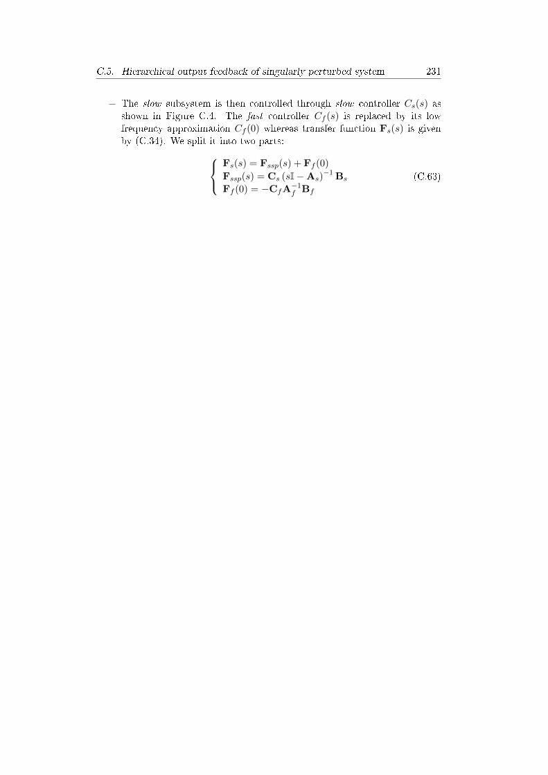
C.5. Hierarchical output feedback of singularly perturbed system 231
− The slow subsystem is then controlled through slow controller Cs(s) asshown in Figure C.4. The fast controller Cf (s) is replaced by its lowfrequency approximation Cf (0) whereas transfer function Fs(s) is givenby (C.34). We split it into two parts:
Fs(s) = Fssp(s) + Ff (0)
Fssp(s) = Cs (sI−As)−1 Bs
Ff (0) = −CfA−1f Bf
(C.63)

232 Appendix C. Singular perturbations and hierarchical control

Appendix D
Introduction to fractional
systems
D.1 Pre-ltering
A prelter Cpf (s) is a controller which is situated outside the feedback loop asshown in Figure D.1.
What is the purpose of the prelter ? Once the controller C(s) is designed
the poles of the feedback loop transfer function Y (s)Rpf (s) are set. Nevertheless the
numerator of this transfer function is not mastered and the zeros of Y (s)Rpf (s) may
cause undesirable overshoots in the transient response of the closed loop system.The purpose of the prelter Cpf (s) is to reduce or eliminate such overshoots inthe closed loop system.
Let Ncl(s) be the numerator of transfer function Y (s)Rpf (s) and Dcl(s) its
denominator:Y (s)
Rpf (s)=Ncl(s)
Dcl(s)(D.1)
The prelter Cpf (s) is then designed such that its poles cancel the zeros ofthe closed loop system, that are the roots of Ncl(s). Furthermore the numeratorof the prelter is usually set to be a constant Kpf such that the transfer functionof the full system reads:
Y (s)
R(s)=
Kpf
Dcl(s)(D.2)
Figure D.1: Feedback loop design with prelter

234 Appendix D. Introduction to fractional systems
As a consequence the transfer function of the prelter reads:
Cpf (s) =Kpf
Ncl(s)(D.3)
Usually constant Kpf is set such that the static gain of Y (s)R(s) is unitary,
meaning that the position error is zero:
Y (s)
R(s)
∣∣∣∣s=0
= 1⇒ Kpf = Dcl(0) (D.4)
D.2 Design steps
The general scheme for the controlled system is provided in Figure D.1 whereCpf (s) is the transfer function of the prelter.
The design philosophy is to set the transfer function C(s) of the controllerand the transfer function Cpf (s) of the prelter in order to force the transferfunction of the full system to have the following expression where Kpf is aconstant gain and Dcl(s) a polynomial formed with the desired closed looppoles:
Y (s)
R(s)=
Kpf
Dcl(s)(D.5)
The design steps of the control loop are the following:
− Design the controller C(s) such that transfer function of feedback loopwithout preltering (Cpf (s) = 1) has the desired denominator Dcl(s).In other words controller C(s) is used to set the poles of the controlledsystem.
− Design the prelter Cpf (s) such that transfer function of the full systemdoes not have any zero:
Y (s)
R(s)=
Kpf
Dcl(s)(D.6)
In other words prelter Cpf (s) is used to shape the numerator of thetransfer function of the controlled system.
Example D.1. Consider a plant with the following transfer function:
F (s) =1
s (s− 2)(D.7)
Obviously the plant is not stable, indeed there is one pole at +2. In order tostabilize the plant we decide to use the following PD controller (we do not usean integral action because the plant F (s) has already an integral term):
C(s) = Kp +Kd s (D.8)

D.3. Pre-ltering design for non-minimum phase feedback loop 235
Furthermore we set the targeted transfer function of the controlled system asfollows (see Figure D.1):
Y (s)
R(s)=
2
s2 + 5 s+ 2(D.9)
The rst step of the design is to set the values Kp and Kd of the PD controllersuch that the denominator of the targeted transfer function is achieved. Transferfunction Y (s)
Rpf (s) (no prelter here) reads:
Y (s)Rpf (s) = C(s)F (s)
1+C(s)F (s)
=Kp+Kd s
Kp+Kd s+s (s−2)
=Kp+Kd s
s2+s (Kd−2)+Kp
(D.10)
The actual denominator will be equal to the targeted denominator as soon asKp and Kd are set as follows:
s2 + s (Kd − 2) +Kp = s2 + 5 s+ 2⇒Kd = 7Kp = 2
(D.11)
Thus transfer function Y (s)Rpf (s) (no prelter here) reads:
Y (s)
Rpf (s)=
Kp +Kd s
s2 + s (Kd − 2) +Kp=
2 + 7 s
s2 + 5 s+ 2(D.12)
Taking now into account prelter Cpf (s) transfer function Y (s)R(s) reads:
Y (s)
R(s)=Rpf (s)
R(s)
Y (s)
Rpf (s)= Cpf (s)
2 + 7 s
s2 + 5 s+ 2(D.13)
Thus transfer function of the controlled system will read Y (s)R(s) = 2
s2+5 s+2as
soon as prelter Cpf (s) is set as follows:
Y (s)
R(s)=
2
s2 + 5 s+ 2⇒ Cpf (s) =
2
2 + 7 s(D.14)
D.3 Pre-ltering design for non-minimum phasefeedback loop
Sometimes the numerator of the feedback loop transfer function Y (s)Rpf (s) has zeros
with positive real part. Such transfer functions with zeros in the right half planein the complex plane, that is with positive real part, are called non-minimumphase transfer functions. As far as the denominator of the prelter is set tothe numerator of the feedback loop transfer function this leads to an unstableprelter, which is not acceptable.

236 Appendix D. Introduction to fractional systems
Suppose that feedback loop transfer function P (s) = Y (s)Rpf (s) has a positive
real zero of order one at s = z > 0, that is P (z) = 0 and dP (s)ds
∣∣∣s=z6= 0. Such
a transfer function can be decomposed as follows1 where Pmp(s) is a minimumphase transfer function:
P (s) =(
1− s
z
)Pmp(s) (D.15)
Using remarkable identity 1 − x2 = (1 − x) (1 + x), the term 1 − sz in the
preceding equation can be expanded using fractional powers of s as follows:
1− sz =
(1−
(sz
)1/2)(1 +
(sz
)1/2)=(
1−(sz
)1/4)(1 +
(sz
)1/4)(1 +
(sz
)1/2)=(
1−(sz
)1/8)(1 +
(sz
)1/8)(1 +
(sz
)1/4)(1 +
(sz
)1/2)= · · ·
(D.16)
That is:
1− s
z=
(1−
(sz
)1/M) log2(M/2)∏
k=0
(1 +
(sz
)2k/M)
(D.17)
where log2(M/2) is the base 2 logarithm of M/2 and M is any numbermultiple of 2.
The positive real zero z can then be partially compensated through the
term DM (s) =∏log2(M/2)k=0
(1 +
(sz
)2k/M)which will appear in the denominator
of the transfer function of the prelter. Indeed it can be shown1 that PM (s) =(1−
(sz
)1/M)Pmp(s) has a weaker non-minimum phase zero at s = z than
P (s) =(1− s
z
)Pmp(s).
The next step consists in approximating the state space fractional systemwith the following transfer function Pf (s) which will appear in the prelter:
Pf (s) =1∏log2(M/2)
k=0
(1 +
(sz
)2k/M) (D.18)
D.4 CRONE approximation of fractional derivative
CRONE (Commande Robuste d'Ordre Non-Entier : this is the Frenchabbreviation for Non Integer Order Robust Control which was introduced byA. Oustaloup2) is a method which enables to approximate the innitedimension fractional lter sαi , αi ∈ (0, 1), by a nite dimension rational
1Practical and ecient method for fractional-order unstable pole-zero cancellation in linearfeedback systems, Farshad Merrikh-Bayat, https://arxiv.org/abs/1207.6962
2A. Oustaloup - La commande CRONE, Hermes, 1991

D.4. CRONE approximation of fractional derivative 237
transfer function Gαi(s) which is provided as follows3:
sαi ≈ Gαi(s) =
(1
ωB
)αi ∏i=+Ni=−N
(1 + s
ωz,i
)∏i=+Ni=−N
(1 + s
ωp,i
) (D.19)
In order to obtain a good accuracy in a frequency range (ωmin, ωmax), polesand zeros are distributed in a broader frequency range (ωA, ωB) dened as afunction of (ωmin, ωmax) and an adjustment coecient σ which is often chosento σ = 10:
ωB = σ ωmaxωA = ωmin
σ
η =(ωBωA
)(1−αi)/(2N+1)
δ =(ωBωA
)αi/(2N+1)
ωz,−N =√η ωA
ωp,i = δ ωz,i i = −N, · · · , Nωz,i+1 = η ωp,i i = −N, · · · , N − 1
(D.20)
We recall that as far as the approximated transfer function Gαi(s) of sαi has
distinct real poles λi, its partial fraction expansion reads:
sαi ≈ Gαi(s) = N(s)D(s) + d
= N(s)(s−λ1)(s−λ2)···(s−λn) + d
= r1s−λ1 + r2
s−λ2 + · · ·+ rns−λn + d
(D.21)
Number ri is called the residue of transfer function Gαi(s) in λi. When themultiplicity of the pole (or eigenvalue) λi is 1 we have seen that residue ri canbe obtained thanks to the following formula:
ri = (s− λi)Gαi(s)|s=λi (D.22)
Now we dene constants bi and ci such that the product bici is equal to ri:
ri = bi ci (D.23)
This leads to the following state-space representation, which is called thediagonal (Jordan) or modal form, corresponding to the approximation of sαi :
sαi ≈ Gαi(s) :
z(t) = Aαi z(t) + Bαi u(t)y(t) = Dαiu(t) ≈ Cαi z(t) + Dαi u(t)
(D.24)
3Comparison between two approximation methods of state space fractional systemsMansouri Rachid, Bettayeb Maamar, Djennoune Said, Signal Processing 91 (2011) 461469

238 Appendix D. Introduction to fractional systems
where:
Aαi =
λ1 0 0
0 λ2...
.... . . 0
0 · · · 0 λn
Bαi =
b1b2...bn
Cαi =
[c1 c2 · · · cn
]Dαi = d
(D.25)
Similarly the Laplace transform of the fractional integration operator Iαiis s−αi . The approximation of the fractional integration operation s−αi can beobtained by exploiting the following equality4:
s−αi =1
ss1−αi (D.26)
Because 0 ≤ 1−αi ≤ 1 as soon as αi ∈ (0, 1), fractional integration operations1−αi can be approximated by a transfer function similar to (D.19). Then thenite dimension rational model is multiplied by 1
s which leads to a strictly properapproximation 1
s s1−αi of the fractional order integration operation s−αi :
s−αi =1
ss1−αi ≈ 1
sG1−αi(s) (D.27)
Because 1s s
1−αi is a strictly proper transfer function, matrix D−αi is null.The state space representation corresponding to the approximation of s−αi
reads:
s−αi ≈ 1
sG1−αi(s) :
z(t) = A−αi z(t) + B−αi u(t)y(t) = Iαiu(t) ≈ C−αi z(t)
(D.28)
D.5 State space fractional systems
Usually the state space model of an integer linear time invariant system is thefollowing:
x(t) = Ax(t) + Bu(t)y(t) = Cx(t) + Du(t)
(D.29)
Where:
4A method for modelling and simulation of fractional systems, Thierry Poinot, Jean-Claude Trigeassou, Signal Processing 83 (2003) 2319-2333

D.5. State space fractional systems 239
Figure D.2: Block diagram of a state-space representation
− x(t) is the state vector, which is of dimension n. The number n of thestate vector components is called the order of the system;
− u(t) is the input of the system;
− y(t) is the output of the system.
State vector x(t) can be dened as a set of variables such that theirknowledge at the initial time t0 = 0, together with knowledge of system inputsu(t) at t ≥ 0 are sucient to predict the future system state and output y(t)for all time t > 0.
Both equations in (D.29) have a name:
− Equation x(t) = Ax(t) + Bu(t) is named as the state equation;
− Equation y(t) = Cx(t) + Du(t) is named as the output equation.
The state equation and the output equation both constitute the state-spacerepresentation of the system.
The block diagram corresponding to the state-space representation (D.29)is shown in Figure D.2.
The corresponding transfer function of the model is given by:
G(s) = C (sI−A)−1 B + D (D.30)
State space representation (D.29) can be extended to fractional case asfollows5:
Dαx(t) = Ax(t) + Bu(t)y(t) = Cx(t) + Du(t)
(D.31)
where:Dαx(t) =
[Dα1x1(t) · · · Dαnxn(t)
]T(D.32)
Denoting by [αk] the integer part of αk the Laplace transform of thefractional Caputo derivative Dαkxk(t) is5:
L [Dαkxk(t)] = sαkL [xk(t)]−[αk]−1∑i=0
sαk−i−1 dixk(t)
dti
∣∣∣∣t=0
(D.33)
5W. Krajewski and U. Viaro, On the rational approximation of fractional order systems,2011 16th International Conference on Methods & Models in Automation & Robotics,Miedzyzdroje, 2011, pp. 132-136. doi: 10.1109/MMAR.2011.6031331

240 Appendix D. Introduction to fractional systems
If all fractional orders are multiples of the same real number α ∈ (0, 1)(commensurate fractionalorder systems), operator Dαx(t) simplies as follows:
Dαx(t) =[Dαx1(t) · · · Dαxn(t)
]T(D.34)
Example D.2. The following example presents a fractional state spacerepresentation and its corresponding transfer function3:
D1.56x1(t)D1.13x2(t)D0.77x3(t)
=
0 1 00 0 1−4 −20 −10
x(t) +
001
u(t)
y(t) =[
4 1 0]x(t)
(D.35)
The corresponding transfer function is the following:
G(s) =s1.56 + 4
s3.46 + 10 s2.69 + 20 s1.56 + 4(D.36)
Denoting by y(t) the output of the system, it is worth noticing that thecomponents of the state vector are the following where y(i)(t) indicates the ith
time derivative of y(t):
x(t) =
y(t)
y(1.56)(t)
y(2.69)(t)
(D.37)
Furthermore D1.56 corresponds to the lower fractional derivative whichappears in the denominator of transfer function G(s) whereas the others terms,D1.13 and D0.77 namely, are obtained by subtracting the consecutive fractionalderivatives which appears in the denominator of transfer function G(s).
Last but not least the fractional exponents which appear in the numerator ofG(s) are the same than those which appear in its denominator.
D.6 Approximation of fractional systems based ondierentiation operator
The approximation of fractional systems based on dierentiation operator isobtained by coupling (D.31) and (D.24):
Dαx(t) = Ax(t) + Bu(t)y(t) = Cx(t) + Du(t)z(t) = Aα z(t) + Bα x(t)Dαx(t) ≈ Cα z(t) + Dα x(t)
(D.38)
Block-diagonal matrices Aα ∈ R(2N+1)·n×(2N+1)·n, Bα ∈ R(2N+1)·n×n, Cα ∈Rn×(2N+1)·n and Dα ∈ Rn×n are obtained from (D.24) as follows:
Aα = diag[
Aα1 · · · Aαn
]Bα = diag
[Bα1 · · · Bαn
]Cα = diag
[Cα1 · · · Cαn
]Dα = diag
[Dα1 · · · Dαn
] (D.39)

D.7. Approximation of fractional systems based on integration operator 241
Equating the expression of Dαx(t) in both equations of (D.38) yields to theexpression of the state space vector x(t) of the fractional model:
Ax(t) + Bu(t) ≈ Cα z(t) + Dα x(t)
⇔ x(t) ≈(A−Dα
)−1 (Cα z(t)−Bu(t)
)≈(A−Dα
)−1Cα z(t) +
(Dα −A
)−1Bu(t)
(D.40)
Finally the approximation of fractional system (D.38) based ondierentiation operator reads:
z(t) = AD z(t) + BD u(t)y(t) ≈ CDz(t) + DDu(t)
where
AD = Aα + Bα
(A−Dα
)−1Cα
BD = Bα
(Dα −A
)−1B
CD = C(A−Dα
)−1Cα
DD = C(Dα −A
)−1B + D
(D.41)
D.7 Approximation of fractional systems based onintegration operator
The inspection of Figure D.2 shows that we may also choose the integral operatorinput x(t) =
∫ t0 w(τ)dτ as the state vector vector and write the corresponding
state space model using the integral function instead of the derivative one. Thisyields to3:
w(t) = A∫ t
0 w(τ)dτ + Bu(t)
y(t) = C∫ t
0 w(τ)dτ + Du(t)
x(t) =∫ t
0 w(τ)dτ
(D.42)
The corresponding transfer function of the model then given by
G(s) = CIs
(I−A
Is
)−1
B + D (D.43)
Denoting by Iαi the fractional integration operator, state spacerepresentation (D.42) can be extended to fractional case as follows3:
w(t) = AIαw(t) + Bu(t)y(t) = CIαw(t) + Du(t)
x(t) = Iαw(t)
(D.44)
where:Iαw(t) =
[Iα1w1(t) · · · Iαnwn(t)
]T(D.45)
The approximation of fractional systems based on integration operator isobtained by coupling (D.44) and (D.28):
w(t) = AIαw(t) + Bu(t)y(t) = CIαw(t) + Du(t)z(t) = A−α z(t) + B−αw(t)x(t) = Iαw(t) ≈ C−α z(t)
(D.46)

242 Appendix D. Introduction to fractional systems
Block-diagonal matrices A−α ∈ R(2N+2)·n×(2N+2)·n, B−α ∈ R(2N+2)·n×n andC−α ∈ Rn×(2N+2)·n are obtained from (D.28) as follows:
A−α = diag[
A−α1 · · · A−αn]
B−α = diag[
B−α1 · · · B−αn]
C−α = diag[
C−α1 · · · C−αn] (D.47)
Using the expression of w(t) provided in the rst equation of (D.46) withinthe expression of z(t) in the third equation of (D.46) and using theapproximation Iαw(t) ≈ C−α z(t) provided in the fourth equation yields:
w(t) = AIαw(t) + Bu(t)⇒ z(t) = A−α z(t) + B−αw(t)
= A−α z(t) + B−α (AIαw(t) + Bu(t))= A−α z(t) + B−αAIαw(t) + B−αBu(t)≈ A−α z(t) + B−αAC−α z(t) + B−αBu(t)=(A−α + B−αAC−α
)z(t) + B−αBu(t)
(D.48)
Finally the approximation of fractional system (D.46) based on integrationoperator reads:
z(t) = AI z(t) + BI u(t)y(t) ≈ CIz(t) + DIu(t)
where
AI = A−α + B−αAC−αBI = B−αBCI = C C−αDI = D
(D.49)
Example D.3. Coming back to Figure D.1, let's consider the following non-minimum phase transfer function:
P (s) =Y (s)
Rpf (s)=
10s− 1
s2 + 1.4s+ 1(D.50)
It is clear that in order to obtain no static error, that is Y (s)R(s) = 1
s2+1.4s+1,
we shall choose the prelter Cpf (s) as follows:
Y (s)R(s) = 1
s2+1.4s+1= P (s)Cpf (s)
⇒ Cpf (s) = 110s−1 = −1
1− s0.1
(D.51)
Obviously Cpf (s) is not a stable system and this prelter cannot beimplemented.
Alternatively we can write P (s) as follows where Pmp(s) is a minimum phasetransfer function:
P (s) =(
1− s
z
)Pmp(s) =
(1− s
0.1
) −1
s2 + 1.4s+ 1(D.52)
Then, choosing for example M = 4 we write:
1− s0.1 =
(1−
(s
0.1
)1/M)∏log2(M/2)k=0
(1 +
(s
0.1
)2k/M)=(
1−(s
0.1
)0.25)(
1 +(s
0.1
)0.25)(
1 +(s
0.1
)0.5) (D.53)

D.7. Approximation of fractional systems based on integration operator 243
From this decomposition prelter Cpf (s) now reads:
Cpf (s) = −1(1+( s
0.1)0.25
)(1+( s
0.1)0.5)
= −(0.1)0.25 (0.1)0.5
(s0.25+(0.1)0.25)(s0.5+(0.1)0.5)
= −(0.1)0.75
s0.75+(0.1)0.25s0.5+(0.1)0.5s0.25+(0.1)0.75
(D.54)
The fractional state space representation corresponding to this transferfunction reads: D0.25x1(t)D0.25x2(t)D0.25x3(t)
=
0 1 00 0 1
−(0.1)0.75 −(0.1)0.5 −(0.1)0.25
x(t) +
001
u(t)
y(t) =[−(0.1)0.75 0 0
]x(t)
(D.55)Figure D.3 shows Bode plots of the two approximating methods for fractional
prelter Cpf (s) with the following setting:N = 4ωmin = 10−2
ωmax = 102(D.56)
Figure D.4 shows the step response of the plant with the rational prelterCpf (s): it can be seen that the non-minimum phase eect has been reduced butthe time response has been highly increased compared with the result obtainedwith a static prelter Cpf (s) = −1 which leads to Y (s)
R(s) = − 10s−1s2+1.4s+1
= −P (s)

244 Appendix D. Introduction to fractional systems
Figure D.3: Bode plots of approximated fractional prelter Cpf (s)
Figure D.4: Step response with approximated fractional prelter Cpf (s)