state-space modelling of residential, commercial and peak demands

Journal of Forecasting, VoI. 6, 97-115 (1987)

State-Space Modelling of Residential, Commercial and Peak Demands*

ROBERT NELSON Georgia Power Company

ABSTRACT The potential use of state-space modelling is evaluated through comparison with the existing multivariate ARMA models currently in use at Georgia Power Company for forecasting its residential sales, commercial sales and peak demand.

KEY WORDS State space Multivariate ARMA Electricity demand

Georgia Power Company (GPC) currently uses a variety of time series, econometric, and end-use methodologies to produce its sales and peak demand forecasts. For forecast horizons 3 years out, however, the company relies exclusively on advanced time series techniques. The models are Box and Jenkins transfer functions referred to as multivariate autoregressive-moving average (ARMA) models. They are driven by a variety of economic, demographic, engineering, and weather time series. Although GPC employs as many as 21 of these models, only three are chosen for review here. The three models are for residential sales, commercial sales, and peak demand. All are monthly time series. These series are chosen for discussion because they demonstrate the full range of data treatments that can be handled with advanced time series techniques such as state space forecasting.

The plan of our study is to select three energy classes and model them as closely as possible using state space techniques to parallel the multivariate ARMA models in current use at GPC. The models and their forecasts will then be compared. The reasons for this approach are as follows: the models in use at GPC are quite sophisticated in application and should provide a rigorous test for state space adaptability; the models being used at GPC are in current official use and can supply a good benchmark test of results; finally the multivariate ARMA methodology is roughly equivalent to state space methods. We shall compare the models and forecasts of the current GPC forecast with the test cases using state space forecasting in FORECAST MASTER.**

* This paper is based upon work undertaken as part of project RP2279 for the Electric Power Research Institute and is published here with permission. ** FORECAST MASTER is a microcomputer based forecasting software package developed for EPRI by Scientific Systems, Inc. (SSI).

0277-6693/87/020097- 19$09.50 Received July 1986 0 1987 by John Wiley & Sons, Ltd.

98 Journal of Forecasting voi. 6, rss. NO. 2

CURRENT METHODOLOGY

Georgia Power Company uses Box and Jenkins ARMA models to forecast electricity sales and monthly peak demand out 3 years. The models are developed using these techniques with varying degrees of complexity. Some are relatively simple multivariate ARMA models with two input series and a stochastic component. Several models employ intervention analysis to account for changes in customer classification. Most models use extensive preconditioning of input series to account for changes in appliance saturations, efficiency, and other time varying relations.

Preconditioning can be described more specifically as follows. Suppose an impact on energy sales such as weather is represented in the model by a constant parameter W. Also suppose the weather impact changes over time so that W ( f ) is the true parameter. The estimated value W will then represent an average value over the estimation period and may be biased in the forecast period. To rectify the situation, we introduce the device of preconditioning the data to accoynt for these time varying effects. Preconditioning operates by selecting a series or index which causes the input series to change its impact on the output to simulate the change that would occur in the parameter. The preconditioned series is then used to build the model. The time varying effect is taken out of the estimation process and put into the input series.

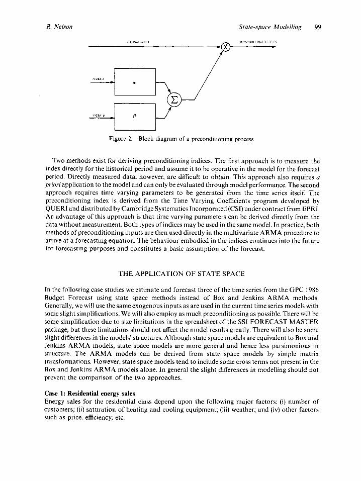
The basic operations which form the building blocks of the preconditioning process are summarized in Figure 1 . The preconditioning process employs the single or combined operations of summation, multiplication, or weighting of the input series. The causal inputs may undergo a series of these modifications. A set of indices may likewise go through a whole tree of these modifications before being applied to the causal input. A possible combination of the various preconditioning operations is represented in Figure 2.

Summation: Two or more causal inputs are summed to a combined output.

Multiplication: Two or more causal inputs are multiplied together to produce a causal output.

Weighting: Two indices are multiplied by weights and summed

-€3 -

Figure 1. Summary preconditioning operations

R. Nelson State-space Modelling 99

i lECC~8DITIONED SERlES

c CAUSALINPUT

Figure 2. Block diagram of a preconditioning process

Two methods exist for deriving preconditioning indices. The first approach is to measure the index directly for the historical period and assume it to be operative in the model for the forecast period. Directly measured data, however, are difficult to obtain. This approach also requires a priori application to the model and can only be evaluated through model performance. The second approach requires time varying parameters to be generated from the time series itself. The preconditioning index is derived from the Time Varying Coefficients program developed by QUERI and distributed by Cambridge Systematics Incorporated (CSI) under contract from EPRI. An advantage of this approach is that time varying parameters can be derived directly from the data without measurement. Both types of indices may be used in the same model. In practice, both methods of preconditioning inputs are then used directly in the multivariate ARMA procedure to arrive at a forecasting equation. The behaviour embodied in the indices continues into the future for forecasting purposes and constitutes a basic assumption of the forecast.

THE APPLICATION O F STATE SPACE

In the following case studies we estimate and forecast three of the time series from the GPC 1986 Budget Forecast using state space methods instead of Box and Jenkins ARMA methods. Generally, we will use the same exogenous inputs as are used in the current time series models with some slight simplifications. We will also employ as much preconditioning as possible. There will be some simplification due to size limitations in the spreadsheet of the SSI FORECAST MASTER package, but these limitations should not affect the model results greatly. There will also be some slight differences in the models’ structures. Although state space models are equivalent to Box and Jenkins ARMA models, state space models are more general and hence less parsimonious in structure. The ARMA models can be derived from state space models by simple matrix transformations. However, state space models tend to include some cross terms not present in the Box and Jenkins ARMA models alone. In general the slight differences in modelling should not prevent the comparison of the two approaches.

Case 1: Residential energy sales Energy sales for the residential class depend upon the following major factors: (i) number of customers; (ii) saturation of heating and cooling equipment; (iii) weather; and (iv) other factors such as price, efficiency, etc.

100 Journal of Forecasting Vol. 6, Iss. No. 2


An effective way to include demographic impacts on residential sales is through a use-per- customer formulation using a separate forecast of residential customers. To model weather, heating and cooling degree days are used. The degree days are average values over the 21 billing cycles in the month. Problems caused by variations in monthly billing cycles are reduced by a use- per-customer-per-billing-day formulation in the current GPC ARMA model. (This detail was omitted in the state space version since it adds little to the accuracy of annual forecasts considered here.)

Weather and population act directly as causal impacts on the system. The data are treated with a first and twelfth difference, hence the models have an imbedded ‘stochastic’ trend picked up from the last year’s historical data. The other factors of appliance saturations, efficiencies, dwelling characteristics, and long term price effects act indirectly by way of modifying the weather inpacts on the system. These factors thus enter the models as indices which precondition the weather series. These indirect impacts enter the cooling load term implicity by way of a time-varying parameter (TVP) index derived empirically from the QUERI/CSI Time-Varying Coefficient program (EPRJ- EA-3143, 198). Their impact is implicit because we know that their total impact results in the time varying parameter index. Multiplicative components of the total can be broken out of the total index for forecasting purposes. Of all the factors mentioned, only three (air conditioning saturation, efficiency, and housing size) can be quantified over the historical period and hence forecasted. All other factors are forecast to be constant at their last estimated historical value. Figure 3 shows a graph of the time varying index over the historical and forecast periods. The heating load term is preconditioned directly by use of a heating appliance saturation index. (The heating saturation preconditioning was omitted in the state space version.) Figure 4 shows a block diagram of the residential model currently in use at GPC.

The stochastic term accounts for all other variations including short term price impacts. Both the current GPC ARMA and the state space models have regular and seasonal moving-average terms. Both models use seasonal and regular differencing to obtain stationarity.

- HISTORICAL ESTIMATE3 - - - FORECAST

1.2

1 . 1

1 .o

YEAR 0.8

71 7 2 73 74 75 76 77 78 79 80 81 02 83 84 85 86 a7 aa a9 90

Figure 4. Residential time varying coefficient index

- T

able

1.

Sum

mar

y of

the

para

met

er e

stim

ates

of

the

shor

t ter

m l

oad

and

ener

gy m

odel

s fo

r the

Geo

rgia

Pow

er C

ompa

ny 1

986

budg

et f

orec

ast

R T R

esid

entia

l"'

W,, =

- 1.

766

W, =

0.40

7 0,

= 0.

518

8, =

0.60

8 18

.1

21

0.64

6 -r

(26.

6)

(21.

7)

(6.6

) (7

.4)

%

8, =

0.34

6 "rl s 4

Cus

tom

er

Coo

ling

Hea

ting

Econ

omic

R

egul

ar

Seas

onal

C

hi

Deg

rees

of

Leve

l of

MA

M

A

squa

re

free

dom

si

gnifi

canc

e 3

recl

assi

ficat

ion

9

Q

(4.4

)

Com

mer

cial

Syst

em p

eak

dem

and

Wo =

-4.3

24

W, =

0.48

2 W

2 = 0.

217

W, =

0.62

1 =

0.7

45

O3 =

0.77

3 (-

16.

5)

(10.

4)

(9.6

) (3

.5)

(9.3

) (9

.2)

lI2 =

0.07

1 (0

.9)

23.6

21

W, =

140

.957

W

, = 5

6.47

0 W

, = 1

76.2

13

8, =

0.90

0 8,

= 0.

686

20.4

22

0.

588

(11.

4)

(4.9

) (3

.0)

(23.

0)

(8.8

)

Not

es:

1) P

aram

eter

est

imat

es f

or R

esid

entia

l are

bas

ed o

n a

use-

per-

cust

omer

mod

el.

2) E

stim

ator

r-s

core

s are

in p

aren

thes

is b

elow

par

amet

er e

stim

ates

.

Tab

le 2

. Su

mm

ary

of t

he p

aram

eter

est

imat

es o

f th

e st

ate

spac

e m

odel

s de

rived

usi

ng th

e FO

REC

AST

MA

STE

R p

rogr

am

Cus

tom

er C

lass

Si

mpl

e Se

ason

al

Seas

onal

M

odel

Ex

ogen

ous

Hea

ting

Var

iabl

es

Pre-

C

hi s

quar

e R

2 di

ffer

ence

A

R

MA

or

der

cool

ing

econ

omic

co

nditi

onin

g (D

OF)

Res

iden

tial S

ales

Y

es

1 .0

0.75

2

CD

D

HD

D

Yes

* 26

.1 (1

4)

0.96

4 -T

C

omm

erci

al S

ales

Y

es

1 .o

0.80

2

CD

D

HD

D

TPY

&

Yes

23

.7 (1

4)

0.94

4 %

3

Shift

p

2

fo

Peak

Dem

and

Yes

1 .0

0.

70

2 T

>80

"F

T<

65"F

TP

Y

Yes

12

.8 (1

4)

0.92

0

* Use

s C

ambr

idge

Sys

tem

atic

s Tim

e V

aryi

ng P

aram

eter

. h,


The current GPC residential use-per-customer-per-day model in equation form is as follows:

Or = woer + w1 H , + (1 - 8, B - 8,B2)( 1 - 8,B’ 2 ) ~ ,

where

0, = (1 - B)(1 - B’2)Ut

H [ = ( 1 - B)( 1 - B’2)HtS, C[ = (1 - B)(l - B”)C,T,

and where U, = undifferenced use-per-customer-per-day; C, = undifferenced cooling degree days per day; H , = undifferenced heating degree days per day; T, = residential time-varying coefficient index; S, = heating saturation index.

Table 1 contains a summary of the parameter estimates and statistics for the residential model as well as all the GPC models described in the other cases.

Figure 5 shows a plot of the historical and forecasted residential use-per-customer as produced by the state space model. One notices the strong seasonal pattern due to weather impacting the system. When one overlays use-per-customer with the preconditioned cooling degree days data as in Figure 6, one is struck by the close fit of the two patterns. Such a close fit was not apparent with the preconditioned heating degree data. The pattern was no more apparent than the data without preconditioning as is shown in Figure 7. This lack of pattern prompted a decision to drop the heating saturation preconditioning from the state space model. The residential state space model is a second order model. This structure in state space results in additional terms to the ARMA version of the model. These terms include lagged variables of second order for both energy and weather. The structure of this model together with some important statistics are shown in Table 2.

The forecasts of residential use-per-customer are compared in Table 3 for both the current Box and Jenkins ARMA model and the state space model. Growth rates for both models are compared.

MONTHLY TIME SERIES DBTB 1911/1

13 F i l3

C

RESUSE - Figure 5. Monthly time series of residential use-per-customer

_--

- *-- ----

-_--

- .- -

.-

:- --

.-


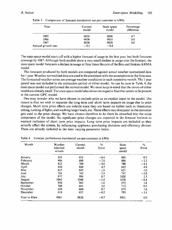
Table 3. Comparison of forecasts (residential use-per-customer in kWh)

Year Current State space Percentage model model difference

1985 1986 1987

Annual growth rate

9828 9898 0.7 9830 9835 0.0 9830 9828 0.0 -0.1 - 0.4

The state space model starts off with a higher forecast of usage in the first year, but both forecasts converge by 1987. Although both models show a very small decline in usage over the forecast, the state space model forecasts a decline in!usage'at four times the rate of the Box and Jenkins ARMA model.

The forecasts produced by both models are compared against actual weather normalized data for 1 year. Weather normalized data are used to be consistent with the assumptions in the forecasts. The forecasted weather series are average weather conditions in each respective month. The 1 year period was not included in the estimation period of either model. As can be seen in Table 4, the state space model out performed the current model. We must keep in mind that the errors of either model are already small. The state space model also shows no negative bias that seems to be present in the current GPC model.

One may wonder why we have chosen to exclude price as an explicit input in the model. The reason is that we wish to separate the long term and short term impacts on usage due to price changes. Short term price effects are volatile since they are based on habits such as thermostat setting, turning of lights, and washing larger loads, etc. These effects may disappear as the customer gets used to the price change. We have chosen therefore to let them be absorbed into the noise component of the model. No significant price changes are expected in the forecast horizon to warrant inclusion of short term price impacts. Long term price impacts are included as they actually affect the system, by influencing appliance purchasing decisions and efficiency choices. These are already included in the time varying parameter index.

Table 4. Forecast performance (residential use-per-customer in kWh)

Month Weather Current YO State % adjusted model Error space Error actuals model

January 955 95 1 - 0.4 960 0.5 February 906 888 - 2.0 886 - 2.2

April 659 689 4.5 692 4.9 May 615 605 - 1.6 62 1 1 .o March 822 784 - 4.6 788 -4.1

June 76 1 742 - 2.4 747 - 1.8

August 1062 1048 - 1.4 1058 - 0.4 July 977 984 0.7 lo00 2.3

September 956 965 1 .o 973 1.8 October 709 69 1 - 2.6 713 0.5 November 659 664 0.7 670 1.6 December 819 817 - 0.2 793 -3.1

Year to Date 9901 9828 -0.7 9901 0.0

Com

mer

cial

Sec

tor-

Ene

rgy

Sal

es M

odel

INIT

IAL

C

ON

DIT

ION

S

NO

OF

BlL

Lltl

G D

AV

P

ER

MO

NII

I \

\

1

CO

OL

ING

DE

GR

EE

‘1

I C

OO

LIN

G F

IL~

EH

D

AY

SP

ER

DA

Y

wl(

i a)(

l ai2

)

NO

NS

TA

TIO

NA

HV

S

UM

h4A

lIU

N F

lLIE

H

111 01

11 a5

i‘

//

I

d

L

1

HE

AT

ING

DE

GR

EE

D

AY

S P

ER D

AY

CO

MM

ER

CIA

L C

US

TOM

EA

G

RO

WTH

IND

EX

tlw

, =

1)

/

,py

K,

4 DvN

AM

IC

/ IN

CO

ME

FlL

lEH

W,II

am1

0’)

)

Figu

re 8

. Bl

ock

diag

ram

of th

e com

mer

cial

sale

s AR

MA

mod

el in

curr

ent u

se b

y G

eorg

ia P

ower

Com

pany

CO

MM

ER

CIA

L E

NE

RG

Y

SA

LES


Case 2: Commercial energy sales Energy sales to the commercial class depend on the following major factors: (i) economic activity; (ii) customer class shifts; and (iii) weather. For the commercial model, real total personal income (TPY) for the state of Georgia is used as a measure of business activity growth.

A number of major shifts involving the commercial class occurred in the mid-70's. In early 1976, industrial customers began to switch to the commercial class in response to rate tariff changes. In September 1977, GPC adopted a revenue code classification based upon the customers' SIC code. The resulting series of shifts between commercial and industrial classes are modelled by use of intervention analysis, i.e. using an indicator variable as an input to model an intervention by some outside factor. The need for the indicator variable will become obvious when we present the time series plots.

Heating and cooling degree days are used as cumulative measure of the weather impact on the system. As with the residential class, they are computed on the average billing cycle basis. Preconditioning of these time series is used because increased weather sensitivity results from new customers growth. Preconditioning with a customer growth index is preferred to a logarithmic transformation since it does not distort the seasonal patterns and decouples winter and summer energy use. (This detail was omitted in the state space version.) The current GPC ARMA model is built on a sales-per-day basis to reduce calendar effects, but this detail was likewise omitted from the state space version. No other preconditioning is used in the commercial model since appliance saturations, appliance efficiencies, and long term price effects have long since reached equilibrium in the commercial class and are assumed to be unchanged in the forecast period. Figure 8 shows a block diagram of the commercial model.

The stochastic term accounts for all other variations that may have occurred in the past and are not forecasted to change in the future including short term price impacts. Like the residential models, both commercial GPC ARMA and state space models employ regular and seasonal moving-average terms as well as regular and seasonal differencing to achieve stationarity.

The current GPC commercial energy sales-per-day model in equation form is as follows:

F, = u,,BS, + ~ , f i , + w2Ct + u$, + (1 - 8, B - Q , B ~ ) ( ~ - e3B12)ct,

where

f, = (1 - B)(l - B'2)Y, 3, = (1 - B)(1 - B'2)S, f i , = ( l -B)(1 -B'2)H,.It C,=(l - @ ( I -B'2)C,.It f t = (1 - B)(1 - B'Z)X,

and where Y, = undifferenced energy sales-per-day; S, = undifferenced customer shift index; H, = undifferenced heating degree days per day; C, = undifferenced cooling degree days per day; X , = undifferenced Georgia Total Personal Income; Z, = commercial customer growth index.

Table 1 contains a summary of the parameter estimates and statistics for the commerical model as well as all the other GPC models described in the other cases.

The plot of the commercial class sales time series in Figure 9 reveals some striking occurrences. One can see a dramatic upward shift in level of sales in 1976, followed by an even more dramatic shift downward in 1977. In both cases the seasonal pattern in sales is preserved. These shifts are caused by the customer migrations and reclassifications mentioned earlier. The plot justifies the intervention treatment given to the GPC ARMA model. This same treatment is carried over to the state space model. As with the GPC ARMA model, the indicator variable is used as a direct input

108 Journal of Forecasting Vol. 6, Iss. No.2

YONTHLY IIHE SERIES DATA 197111 199811

12

c 11

18 ; I

9 E

5

Figure 9. Commercial sales for Georgia Power Company

1911/1 MONTHLY TIME SERIES DATA

199811

w 28

Figure 10. intervention variable

Commercial sales plotted with Georgia real total personal income and a customer shift


in the state space model. To see what that treatment is in graphical terms, one must look at Figure 10. This figure shows an overlay of three time series; commercial energy sales, a dummy index to account for customer migrations and reclassifications, and Georgia state total personal income. One can see that the customer shift index runs contrary to the shift in sales and should yield a negative coefficient in the models. Buried under all these complex movements, i.e. seasonal movements due to weather and customer shifts, one can make out dips and surges due to changes in business activity. These movements are subtle, however, and are best tested through the model estimation process. The use of T-statistics would be very useful here, but are not available in FORECAST MASTER at present. The sign of the TPY coefficient indicates trouble in that variable, although complicated model ldynamics may be getting in the way. A search for a better indicator variable may be necessary. The seasonal movements of commercial energy sales can be seen overlayed by the weather series in Figures 11 and 12. Figure 11 shows sales with cooling degree days, and Figure 12 shows sales with heating degree days. The patterns revealed by overlaying weather on sales do not show as tight a correspondence as with the residential class and may indicate a need for more work on the model. However, the T-statistics for the weather terms as seen in Table 1 of the GPC ARMA model indicate strong significance even if only half as great as in the residential model.

The structure of the state space commercial model is shown in Table 2. The FORECAST MASTER indicated a second order model be used, and we chose this over the first order model to produce the forecast.

Table 5 shows a comparison of the current GPC 1986 Budget forecast produced by the ARMA model and the state space test case. The growth rate for the state space forecast is nearly the same as the ARMA model. The state space forecast starts at a much lower level than the ARMA model. To resolve lthe issue of which forecast is better we refer to Table 6, a comparison of forecasts against 1 year of weather normalized actual sales data. Unlike the residential case, the state space model

MONTHLY IIME SERIES DAIA 191M 19984 12 I- I

5

, 3

3 ;

0

COMNWH - COMCDD _.__. Figure 11. Commercial sales plotted with cooling degree days

1 10 Journal of Forecasting Vol. 6, Iss. No.2

MONTHLY IIME SERIES DATA r97i/1 1990/1

I

l2 t

COMMWH - COMHDD ___.. Figure 12. Commercial sales plotted with heating degree days

performed poorly compared to the ARMA model. The current ARMA model missed 1.2% on the low side in the first 6 months of the year. It deteriorated further in the last part of the year. The state space model performed badly in the first 6 months with a cumulative error of 2.5%. It deteriorated very badly during the second 6 months. The poor performance of both models may be explained in part by economics. A predicted economic downturn in the latter part of 1985 did not materialize (see Figure 14). Commercial construction continued into 1986 at a brisk pace, driving the growth of commercial energy sales.

In the series considered in this report, some are seasonal but stationary such as the weather data. Other series are nonstationary and nonseasonal such the economic time series. Still other series are both nonstationary and seasonal such as the energy time series. Yet all time series are treated the same way regardless of the data series’ behaviour. All time series are given both a regular and a seasonal difference. It would seem that many time series modelled here are overdifferenced in some way. We justify this treatment as follows: Individual treatment of each series and uniform treatment are both acceptable. Any linear transformation of the data should not affect the model results so long as the model was correctly specified in the first place. However, a uniform treatment

Table 5. Comparison of forecasts (commercial energy sales in GWh)

Year Percentage model model difference

Current State space

1985 1986 1987

11594 11372 - 2.0 12083 11827 - 2.2 12584 12256 - 2.7

Annual growth rate 3.9 3.8

R. Nelson State-space Modelling 1 11

Table 6. Forecast performance (commercial energy sales in GWh)

Month Weather adjusted actuals

Current model

January February March April

June July August September October November Decem her

Year to Date

May

95 1 969 886 856 906

1029 1106 1139 1121 1000 905 987

11853

969 926 887 872 877

1001 1098 1097 1091 953 865 958

11594

YO State Yo Error space Error

model

1.9 937 - 1.5 - 4.4 923 - 4.8

0.1 877 0.1 1.9 859 0.4

- 0.3 88 1 - 2.8 - 2.7 98 1 - 4.7 - 0.7 1037 - 6.2 - 3.7 1074 - 5.7 - 2.7 1061 - 5.4 - 4.7 962 - 3.8 - 4.4 878 - 2.9 - 2.9 919 - 6.9

- 2.2 11373 -4.0

of the data series lends the models greater structural interpretability to the forecaster. This is the primary motivation for choosing this approach to data differencing.

Case 3: Monthly peak demand Monthly peak demand depends on the following factors: (i) weather on day of peak; (ii) appliance saturation and efficiencies; (iii) level of economic activity; and (iv) population and other factors.

The peak demand models compared here use temperature indices at or around the time of peak to account for weather impacts on the system. The cooling index uses weighted 4 p.m. and 1 a.m. temperatures from the day of peak and the previous day to capture the build up of load seen during a typical hot spell when the peak is set. The heating index is simply the 7a.m. day of peak temperature for the winter peak. The preconditioning is complex as seen from Figure 13. The state space version retains only the time-varying coefficient index used in the GPC current version of the model. Total personal income (TPY) for the state of Georgia is used to capture growth in peak demand. As with the residential model, factors other than weather, and in this case TPY, are captured in the preconditioning indices.

The stochastic term accounts for any other variations including short term price impacts. Both the current GPC ARMA and the state space models have regular and seasonal moving-average terms and differencing.

The current GPC peak demand model is as follows:

P, = woe, + WllFj, + w2Pt + (1 - 8,B)(1 - B2B'2)a,

P, = (1 - B)(1 - B'2)Yt c, = (1 - B)(1 .- B'2)CtT,(3'

P( = (1 - B)(l - B'2)Xr

where

H , = ( 1 - B)(1 - B'2)H,(0.8914S,I,"' + 0.10861,(2')

and where U, = = undifferenced use-per-customer-per-day; C, = undifferenced cooling degree days per day; H , = undifferenced heating degree days per day; A', = undifferenced Georgia total

Peak

Hou

r D

eman

d M

odel

c c

h,

VIW

lE N

OIS

E

ST

OC

HA

SlI

i.

I IL

TtH

\ T

IME

V

AR

YIN

G C

OE

FF

ICIE

NT

IN

DE

X

'-\ -

UY

NA

MlL

LO

OL

INb

Fi

b 1

tR

HE

AT

ING

SA

TU

RA

TIO

N

'1'''

w I

I 01

1 I

0'2

1

MO

NT

H1

"YN

AM

IC H

EA

TIN

G

FIL

TE

R

IND

EX

RE

SID

EN

TIA

L C

US

TO

ME

R

'I4

''

GR

OW

TH

IND

EX

CO

MM

ER

CIA

L C

US

TO

ME

R

GR

OW

TH

IN

DE

X

PER

DA

Y l

CA

l CN

DA

R

MO

NT

H)

(~

,II

BIII

n"1

I -

' H

EA

TIN

G D

EG

RE

E O

AV

S

H.

INIT

IAL

C

ON

LJIII

ON

S

I

SU

MM

AT

ION

FI

LTE

R

Ill

0111

8'2

11

'

PtA

K llu

llll

UC

MA

NLJ

Figu

re 1

3.

Bloc

k di

agra

m o

f th

e pe

ak d

eman

d A

RM

A m

odel

in c

urre

nt u

se b

y G

eorg

ia P

ower

Com

pany


personal income; T, = residential time varying coefficient index; S, = heating saturation index; and 1, = customer growth index.

Table 1 contains a summary of the parameter estimates and statistics for the peak demand model as well as all the other GPC models described in the other cases.

The plot of monthly total system peak demand is shown in Figure 14 together with an overlay of total personal income for the state. While both time series show the same general upward trend, the coincidence of cause and effect is not all that striking. The T-statistics for the ARMA Model, however, show some strength of correlation, again underscoring the need for this sort of statistic in state space forecasting (currently missing in FORECAST MASTER). We will keep the TPY term intact in the state space model as in the ARMA model and assume on faith that it is significant. Figures 15 and 16 show the peak data overlaid by weather. Note here that the time varying component for peak is operative on the cooling index only during the months of June, July, and August. This is when the peak is most sensitive to weather. The other months are not as sensitive to weather. Examination of the peak to weather patterns does not reveal as strong a correspondence as in the residential usage data. This supports the belief that most conservation occurs off peak.

The structure of the state space peak demand model is shown in Table 2. FORECAST MASTER indicated a second order state space model and this yielded the best overall model. Ofall the complex preconditioning used in the GPC ARMA model only the time varying coefficient index was used. Work sheet size limitations were the reason for this change.

A comparison of ARMA and state space forecasts is shown in Table 7. The ARMA forecast is the 1986 Budget Forecast of annual system peak demand. There are some slight differences in growth rates, and the state space model forecast at a higher level throughout the forecast horizon. However, the performance of the state space model is superior to the ARMA model. The ARMA model yielded a forecast of 12424 MW for the summer of 1985. The weather normalized summer peak for 1985 was 12687 MW. This gives an error of 2.1 YO on the low side for the official 1986

197111 HONTHLY T I M SERIES DATA

1999/1

35 4 ? i

38 h

!!

t

t 25 f I

28

PEAK - TPY _..._. Figure 14. Peak demand plotted with Georgia total personal income

c

L

P

PE

-K

1

E-

88

3

c

c

m

m

Q)

N

.p

c

-

-0

-

- ---I- --

-1

P

__

I

c


Table 7. Comparison of forecasts (annual peak demand in MW)

Year Current State space Percentage model model difference

1985 1986 1987

Annual growth rate

12424 12657 1.8 12879 13101 1.7 13336 13568 1.7

3.4 3.2

Budget Forecast. The state space forecast gave a summer peak of 12657 MW, or an error of 0.2% on the low side. Since the conclusions reached here are based on one application, they clearly must be treated with reservation.

CONCLUSIONS

The state space technique appears to be an acceptable alternative to the Box and Jenkins technique for forecasting electricity sales data. The state space approach is easier to apply since the model structure is determined by the technique itself. However, the resulting model is more complex and is not as easy to understand at a glance. Nor is it as easily explained as the simpler Box and Jenkins forms.

Author’s Biography: Robert F. Nelson is a Senior Economic Analyst in Georgia Power Company’s Forecasting Department. He holds an M.S. degree in Electrical Engineering from the George Washington University. His current interests include applied state space forecasting and market penetration of new technologies.

Author’s address: Robert F. Nelson, Economic Services Organization, Georgia Power Company, Post Office Box 4545, Atlanta, Georgia 30302, U.S.A.

state-space modelling of residential, commercial and peak demands

Documents