statistical admission control in multi-hop cognitive radio...
TRANSCRIPT
Statistical Admission Control in Multi-Hop CognitiveRadio Networks
Guillaume Artero Gallardo12, Gentian Jakllari1, Lucile Canourgues2, Andre-Luc Beylot1
1Department of Telecommunications and Networks, ENSEEIHT, University of Toulouse
2Rockwell Collins France
{guillaume.arterogallardo, jakllari, beylot}@enseeiht.fr
Technical Report
Abstract
Cognitive radios promise to revolutionize the performance of wireless networks. Re-alizing this promise, however, requires revisiting and/or reinventing many of the currentnetwork architectures, protocols and policies. In this work we focus on Quality of Servicerouting and more specifically, admission control. We consider a multi-hop cognitive radionetwork where every node is equipped with multiple transceivers. In addition, becausethe research and development of a widely accepted MAC protocol for these networks isstill ongoing, we assume a bare-bones TDMA protocol at the link layer. We show that forthe network considered the problem of computing the available bandwidth of a given path– necessary for admission control – is NP-Complete. The reason for this result is thatcomputing the available bandwidth of a path requires allocating capacity on every hop ofthe path such that the realized end-to-end throughput is maximized – and that is an in-tractable problem. Instead of working on an approximation algorithm we follow a differentapproach. We use a simple scheduling heuristic: Each node selects the slots on which totransmit by choosing at random among those available. Randomized scheduling is widelyused because of its simplicity and efficiency. However, computing the resulting averagethroughput over a multi-hop path has been an open problem. We solve this problem anduse the solution as a vehicle for BRAND, an algorithm for computing the maximum real-izable throughput – the available Bandwidth – with RANDomized scheduling of a multihop path in a cognitive radio network. We show that BRAND can be implemented ina distributed fashion and thus integrated by almost all routing approaches. An exten-sive numerical analysis demonstrates the accuracy of BRAND and its enabling value inperforming admission control.
1 Introduction
Currently, the wireless spectrum is tightly regulated by centralized authorities, such as the FCCin the United States. Operating on wireless spectrum requires either applying for an exclusivelicense by the respective governmental authority or, requires using select frequencies, like thosein the ISM band, that are freely available. However, driven by unprecedented demand forwireless capacity and increasing evidence that a lot of the licensed spectrum is underutilized [1]policymakers and technologists have joined voices in calling for a shift from an exclusive and
1
static mode of allocating wireless spectrum to one that is more adaptive to user traffic [2, 3, 4].The US President’s council of advisors on science and technology in its 2012 report [5] concludesthat, when it comes to the wireless spectrum, ”the norm should be sharing, not exclusivity”,and estimates that a new architecture and a corresponding shift in practices could multiply theeffective capacity of the spectrum by a factor of 1,000.
This shift from the regulating authorities, coupled with the emergence of the cognitive radionetwork concept [6] as the enabling technology, has ignited tremendous interest in cognitive ra-dio networks that are capable of intelligently exploiting the wireless spectrum [1]. Nevertheless,considering the architectural changes required, a lot of technical and policy challenges need tobe ironed out before this vision can turn into reality [4, 7]. Towards this, a lot of effort has beenput in developing solutions for cognitive radio networks at the physical, link and the routinglayers [8, 9, 10, 11, 12, 13, 14, 15, 16]. The IEEE 802 standards committee has also gotteninvolved [17]. However, we are far from having all the answers.
One particular question that has not been addressed is that of QoS routing and morespecifically, admission control in multi-hop cognitive radio networks. Provided a newly arrivingtraffic session, before admitting it, we would like to know whether there is enough bandwidthfor serving the session’s traffic demand. The question can be answered by first computing thebandwidth currently available on the path from the source to the destination node. This isthe focus of this work. In particular, we focus our attention on the problem of computingthe available end-to-end bandwidth for a cognitive network where every node is equipped withmultiple transceivers1 and the link layer uses a TDMA protocol [19, 20, 17, 21, 22].
Computing the end-to-end bandwidth is not a new problem[23]. However, there are tworeasons for revisiting it. First, there is no practical solution widely accepted for legacy2 TDMAwireless networks [24]. Second, the cognitive radio architecture makes the problem non-triviallydifferent. The main reason for this is the existence of the so called primary-secondary hierarchy3.In issuing its landmark ruling [2], permitting the use of unlicensed devices in the UHF spectrum,FCC required that unlicensed devices - the secondary users - do not interfere with incumbents- the primary users. Thus, the end-to-end bandwidth in these networks will be conditionednot only by the interference between peers, as is the case in legacy wireless networks, but alsoby a different kind of interference: Primary users, as their prerogative, will access the channelwithout making any effort to avoid interfering with secondary users. In addition to the primaryuser interference, another distinguishing feature of these networks is that cognitive radios, intheir pursuit of available spectrum, may access different frequency bands and use differentchannel widths [9]. This will lead to network links with widely varying capacities. Multi-ratelinks can also be seen in legacy networks, such as IEEE 802.11, but in cognitive networks theyare a fundamental feature that has to be taken into account by any bandwidth calculationalgorithm.
In this work, we model and analyze the problem of computing the available end-to-endbandwidth in multi-hop cognitive radio networks. We provide a solution to the problem that is
1The cost and size of transceivers is rapidly dropping with spectrum remaining the bottleneck. Accessingwide parts of spectrum will be best served by multiple transceivers [18].
2We refer to non-cognitive architectures as legacy.3In the future, if the vision of a fully dynamic spectrum sharing becomes a reality, we will probably see more
than two classes of users and respective channel access priorities. However, for the moment we focus on thebasic case of a two-class hierarchy.
2
practical and yet takes into consideration the particularities of cognitive radio networks. Ourcontributions can be summarized as follows:
• We formally define the problem of computing the available end-to-end bandwidth of apath in TDMA based multi-hop cognitive radio networks and show that, as in the caseof legacy networks, the problem is NP-Complete.
• We introduce BRAND, a heuristic for estimating the available end-to-end bandwidth.BRAND works by using a randomized slot scheduling and computing the average end-to-end throughput for all possible traffic demands. The maximum over all the computedthroughput values is returned as the available end-to-end bandwidth.
• As part of BRAND, we introduce a novel, linear time algorithm that can compute theaverage end-to-end throughput of a multi-hop path resulting from using randomized slotscheduling on every link of the path. Randomized scheduling is widely used because of itssimplicity and efficiency [25]. However, computing the end-to-end throughput resultingfrom its application on a multi-hop path, to the best of our knowledge, was an openproblem prior to this work.
• We show that BRAND can be implemented in a distributed fashion and can be used bymost routing protocol approaches.
We perform an extensive numerical analysis of BRAND in general and the throughputcomputation algorithm in particular. Our analysis demonstrates the accuracy of our algorithmin computing the average end-to-end throughput as well as BRAND’s capability in providingcorrect information for performing admission control in the presence of primary users andmulti-rate links.
The rest of the paper is organized as follows. In Section 2, we describe in detail the systemmodel, including how we model the effect of the primary user. In Section 3, we formally definethe bandwidth calculation problem and introduce BRAND. In Section 4, we show how BRANDcan be implemented in a distributed fashion while in Section 5 we discuss the performanceevaluation. In Section 6, we discuss some related work. Finally, we conclude the paper inSection 7.
2 Model and Preliminaries
In the following, we describe in detail how we model a multi-hop, multi-transceiver cognitiveradio network.
2.1 Network Model
We model a multi-hop cognitive radio network as a graph G = (V,E), where V is the set ofnodes and E the links. We assume that the network is composed of only symmetric links,that is, there exists an edge between two vertices vi and vj if and only if nodes ni and nj areable to correctly communicate with each other. Every cognitive radio node is equipped witha constant number of half-duplex transceivers, each capable of sensing and transmitting on B
3
predefined orthogonal wireless channels [18]. All the channels can offer different data rates. Anadditional transceiver could be used for control signaling. We assume the channel assignmentis performed by a spectrum allocation protocol [26] and focus on estimating the available end-to-end bandwidth once such assignment is completed. The only assumption we make aboutthe frequency assignment algorithm is that only one frequency channel is assigned between aparticular pair of neighboring nodes.
2.2 Cognitive Channel Access
As a prerequisite for using licensed spectrum, cognitive radios are not to use the channel when itis in use by the respective licensed user. In literature, this is referred to as a secondary-primary4
hierarchy, with the primary (licensed) user having strict priority in accessing the channel. Inthis setting, the key novel challenge when designing a channel access protocol is maximizing therealized capacity of the cognitive radio without adversely affecting the Primary User, despitenot knowing the latter’s communication pattern [27, 28, 29]. In response to this challenge, manynew MAC protocols for cognitive radio networks have been proposed [9]. For all the diversityin the proposed solutions, one thing underlying all protocols is the need for a sensing modulewhose responsibility is identifying when the cognitive radio may be interfering with a primaryuser. In its basic form, this module relies on physically sensing the channel [4] periodically tolook for primary user activity. When possible, the physical sensing can be complemented by adatabase of well known primary users [30].
Given the functionality of the sensing module, a MAC protocol for cognitive radio networksneeds to provide periods of network silence to be dedicated to sensing for primary user activity.What is more, since the activity of the primary user may be completely unknown, these dedi-cated sensing periods need to be periodic. This means that, at given time intervals, all cognitiveradios in the network will stop from generating any traffic, and instead, focus on sensing. Arequirement that can be easily accommodated by a TDMA protocol. Indeed, a majority of theMAC protocols proposed for cognitive radio networks [19, 20, 17, 21, 22], including the IEEE802.22 MAC [17], are based on TDMA. Nevertheless, some solutions based on random accesshave also been proposed [11, 31, 32, 10].
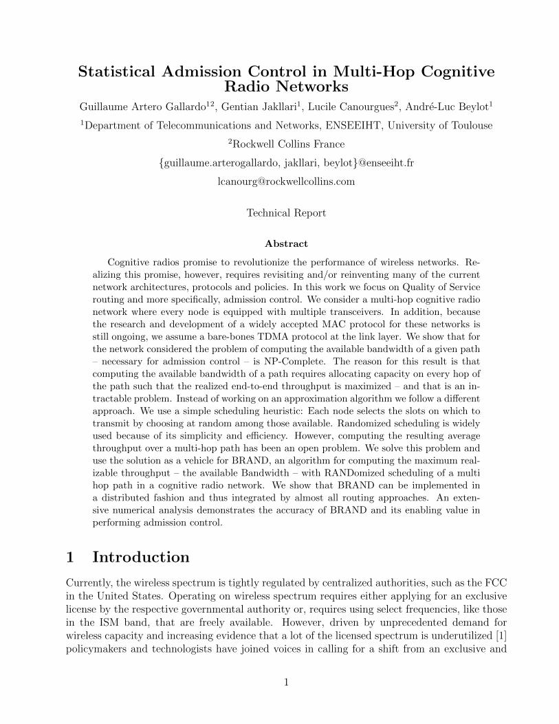
While there is no clear winner yet among the MAC protocols proposed, we believe a deter-ministic medium access protocol will better serve an architecture where multiple technologiesshare the same spectrum and synchronization is required for the sensing. Therefore, we adopta system in which a TDMA MAC with frame size S is implemented on every assigned channel.Every time-slot is started by a sensing period as illustrated in Figure 1. When a node needs totransmit data to a neighboring node, it can access the medium by reserving time-slots on thefrequency channel assigned to this particular link. For ease of presentation, we refer to the pair(channel, timeslot) simply as, a slot.
2.3 Interference in Cognitive Radio Networks
There are two kind of interference sources in a cognitive radio network. There is the interferencefrom other cognitive radios in the same interference domain, usually referred to as secondary-
4For the rest of the paper, we will use the terms primary user/secondary user, primary/secondary and PU/SUinterchangeably.
4
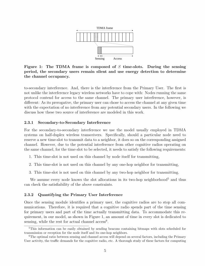
TDMA frame
AccessSensing
Figure 1: The TDMA frame is composed of S time-slots. During the sensingperiod, the secondary users remain silent and use energy detection to determinethe channel occupancy.
to-secondary interference. And, there is the interference from the Primary User. The first isnot unlike the interference legacy wireless networks have to cope with: Nodes running the sameprotocol contend for access to the same channel. The primary user interference, however, isdifferent: As its prerogative, the primary user can chose to access the channel at any given timewith the expectation of no interference from any potential secondary users. In the following wediscuss how these two source of interference are modeled in this work.
2.3.1 Secondary-to-Secondary Interference
For the secondary-to-secondary interference we use the model usually employed in TDMAsystems on half-duplex wireless transceivers. Specifically, should a particular node need toreserve a new time-slot to transmit data to a neighbor, it does so on the corresponding assignedchannel. However, due to the potential interference from other cognitive radios operating onthe same channel, for the time-slot to be selected, it needs to satisfy the following requirements:
1. This time-slot is not used on this channel by node itself for transmitting,
2. This time-slot is not used on this channel by any one-hop neighbor for transmitting,
3. This time-slot is not used on this channel by any two-hop neighbor for transmitting.
We assume every node knows the slot allocations in its two-hop neighborhood5 and thuscan check the satisfiability of the above constraints.
2.3.2 Quantifying the Primary User Interference
Once the sensing module identifies a primary user, the cognitive radios are to stop all com-munications. Therefore, it is required that a cognitive radio spends part of the time sensingfor primary users and part of the time actually transmitting data. To accommodate this re-quirement, in our model, as shown in Figure 1, an amount of time in every slot is dedicated tosensing, while the rest for actual channel access6.
5This information can be easily obtained by sending beacons containing bitmaps with slots scheduled fortransmission or reception for the node itself and its one-hop neighbors.
6The optimal ratio between sensing and channel access will depend on several factors, including the PrimaryUser activity, the traffic demands for the cognitive radio, etc. A thorough study of these factors for computing
5
If during the sensing period a primary is identified, no communication will take place in theaccess part of the slot. Otherwise, the cognitive radio is free to access the channel.
Note, however, that sensing is not perfect. It can very well happen that, while no primaryuser is identified during the sensing period, a primary user does become active for the whole orpart of the the access time. When this happens, the exact consequences on whatever secondaryuser transmissions going on will vary depending on the location and the power strength ofthe primary user. We follow a somehow pessimistic assumption: A primary, when active, willinterfere destructively with any secondary communication taking place in its range7.
If we denote with η the part of the slot access time that will be available to the secondaryuser, based on the reasoning so far, we have:
η = P[sensing the channel idle]
× (Fraction of Access Time Free of PU)
Denoting with ul the probability of a primary user becoming active on link l during a particularslot, the fraction of the slot access time available to the secondary on link l can be computedas follows:
ηl = (1− ul)2 (1)
Taking into account the sensing time, the fraction of slot duration, fl, available for secondary-to-secondary communication is:
fl = ηl ×Taccess
Tsensing + Taccess(2)
The simplified formula for Equation 1 can be formally proved by modeling the PU’s activitywith an alternative ON/OFF process [28, 29]. The details of the proof can be found in theAppendix.
Equation 1 quantifies the effect of two things on the capacity for the secondary. First, theinterference from the primary, who as the owner of the frequency is bound by no protocol to tryto avoid interference with an ongoing secondary communication. And second, the mechanismput in place, i.e. sensing, for satisfying the requirement of doing no harm to the primary. Notethat, for a primary activity of 10%, the secondary user will not realize more than 81% of theslot access time capacity. At first, one might think that the secondary should instead be ableto reach 90%. The explanation for the 9% loss is the sensing. A primary could be active duringthe sensing period but not so during the access time and yet, the secondary will not use theaccess time, leading to unnecessary loss of capacity.
the optimal sensing time is beyond the scope of this paper. However, the correctness of our scheme does notdepend on the exact values of sensing and access times.
7We assume that if a secondary can sense a primary user then the particular secondary is in the interferencerange of the primary user.
6
3 Computing the available end-to-end bandwidth of a
path
3.1 Problem Definition
Let the demand d, expressed in bits per second, refer to the amount of end-to-end bandwidthdemanded by an application. Before admitting to route this demand, we first would like toknow whether this demand can be satisfied end-to-end. This question can be answered bysimply computing the currently available end-to-end bandwidth of the path to the destination.
Definition 1. The available end-to-end bandwidth of a path is the maximum amountof data, in bits per second, that can be currently transported over the path.
Remark 1. Unlike the maximum end-to-end bandwidth, the available bandwidth is time sensi-tive and depends on the current conditions and allocations in the network. If there is no otherongoing traffic in the network and there is no primary user activity, the available bandwidth isequivalent to the maximum path bandwidth.
Remark 2. The admission control problem could alternatively be framed as one of computingthe path with the maximum available bandwidth. However, this would require implementing anew routing protocol for this purpose. What is more, given that we want to solve this problemonline, as the traffic sessions arrive in real-life, it is not clear that, overall, it would lead tomore sessions being admitted. Thus, we opted for an approach that can be added to any availablerouting protocol that, once computing the routes based on whatever metric it considers crucial,can simply asks us for the available bandwidth on a particular path.
Constructing the formal problem definition: A path is modeled as a directed chainn1 → n2 · · · → nNH+1 composed of NH hops. For ease of presentation, we denote a linkni → ni+1 as li. The bit-rate8 of every link is denoted by φi and, for every link, the maximumTDMA frame size is S slots. To take into account the effect of self-interference, that is, links onthe same path interfering with each other, we use the exponential notation (j) to specify that theconsidered quantity is evaluated just before node nj on the same path does its allocations. Using
this convention, we define A(j)i as the number of slots available at node ni for communication
on the link li just before nj does its own allocations.Let us analyze the network behavior when admitting a new flow with demand d. The first
node on the path, n1, converts the flow demand, d, to the required number of slots, r1, to beallocated on the first path link, l1. The number of required slots will depend on the demand, thelink bit-rate, φ1, the TDMA frame size, S, as well as the primary user interference (quantifiedin Section 2.3.2, Equation 2):
r1 =
⌈d
φ1 × f1× S
⌉Let ai denote the number of slots specifically allocated on every hop i ∈ {1, .., NH} for servicingthis flow. For every hop this number will depend on both the demand and, how many slots are
8How the MAC layer computes the bit-rate on a particular link is orthogonal to our contribution. A potentialapproach could be combining the physical bit-rate with the ETX metric.
7
actually available for new allocations. Thus, for the first hop we have a1 = min(r1, A(1)1 ). If
a1 < r1 the demand on the second link will be lower than the original demand, d. To distinguishthe two, we denote the demand on the second link, which depends on the allocation on the firstlink as, d1. Rigorously speaking, d1 = min
(d, a1 × (φ1×f1
S)), where the quantity by which a1 is
multiplied is the capacity of a single slot on the first link. We can generalize these results forany hop, i > 1, as follows:
ri =
⌈di−1φi × fi
× S⌉
(3)
ai = min (ri, A(i)i ) (4)
and
di = min
(di−1, ai ×
(φi × fiS
))(5)
Thus, for a specific demand d, the realized end-to-end throughput is min (d1, d2, ..., dNH) =
dNH, since di ≥ di+1. This analysis gives us a way for tackling the main problem, computing
the available end-to-end bandwidth.
Problem 1. Computing the available end-to-end bandwidth of a path is equivalent to solvingthe following optimization problem:
maxd∈Id
dNH(d) (6)
where Id = [0,min(φ1, φ2, ..., φNH)].
The optimization problem thus defined leads to two observations:
1. The realized end-to-end throughput, dNH(d), given a demand, d, obviously depends on d.
2. dNH(d) depends on how the slots are allocated on every hop.
Why computing the available end-to-end bandwidth is challenging: To illustratethe implications of the above observations and how challenging the above optimization problemis, let us consider the following toy example. Consider the first three nodes, A, B, C of amulti-hop path and let us assume they all have assigned the same channel, which puts themin the same interference domain. The TDMA frame consists of ten slots. In node A slots1,2,5,6 are available for transmitting and receiving, in node B, slots 2,5,6 are available fortransmitting and receiving while slot 1 is available for receiving only9, and in node C all slotsare available for transmitting and receiving. If the demand d is such that four slots are requiredfor satisfying it, the first node, A, will allocate slots 1,2,5,6. Since nodes B, C are in the sameinterference domain, node B will not be able to transmit to node C on any of its slots availablefor transmitting. This will result in a zero end-to-end throughput. Now let us consider that thedemand d is such that two slots are required for satisfying it. In this case node A has
(42
)ways
to chose the two slots for allocation out of the four available. While for node A all choices are
9It can happen that a node scheduled to receive on slot 1 is in the same interference domain with B but notA.
8
equivalent, that is not the case for nodes B and C and ultimately, the end-to-end throughput.If A allocates slots 2 and 5, node B will be left with only one slot, slot 6, to use for forwardingtraffic to node C. If, instead, A allocates slots 1,2, node B will be left with two slots, slots 5,6,for forwarding traffic.
Clearly, the way slots are allocated on every node will have an impact on the realized end-to-end throughput. What is more, the number of possible schedules can grow exponentiallywith the number of nodes on the path. This leads to the following result.
Theorem 1. Computing the available end-to-end bandwidth of a path in a TDMA-based multi-hop cognitive radio networks with multiple transceivers is NP-complete.
Proof. The proof is straightforward so we provide a sketch. We show that our problem isNP-Complete by reducing the problem of computing the maximum path bandwidth in a single-channel TDMA-based multi-hop network, therein referred to as P2, to our problem, thereinreferred to as P1. To this end, we consider the instance of P1 where a same channel with aconstant data rate is assigned on every link along the path and the probability of primaryactivity on all links is zero. Solving P1 actually consists of solving one instance of P2. Since P2
has been shown to be NP-complete[23], that concludes the proof.
3.2 BRAND: An Approach for Estimating the Available End-to-End Bandwidth of a Path
With the problem of computing the available end-to-end bandwidth being NP-Complete, theoverwhelming approach in literature has been to design a scheduling heuristic. We follow adifferent approach. We select a specific slot scheduling algorithm and focus on computing theavailable end-to-end bandwidth resulting from applying this particular algorithm. As schedulingalgorithm we select the randomized scheduling [25]: when a node needs to assign a certainnumber of slots, it will select at random among those available.
Therefore, our high-level algorithm for estimating the available end-to-end Bandwidth withRANDom scheduling, BRAND, works as follows. For every possible demand d, the necessaryslots are allocated at random among those available on every link and the resulting end-to-endthroughput is computed. By Equation 6, the available end-to-end bandwidth is simply themaximum end-to-end throughput realized over all possible demands d.
Algorithm 1: BRAND (Available Bandwidth with RANDom Scheduling)
Output : The available end-to-end bandwidth1 : begin2 : for every possible demand d do
//Use Random Scheduling
3 : avThput← Compute-averageThput (d);4 : if avThput > AvailBW then5 : AvailBW ← avThput;
6 : Return AvailBW ;
9
channel 1
1 2 3 4 7 5 6 8
channel 2 channel 3
5 h
ops
32 timeslots
channel selected for communication by the routing protocol
channel 4
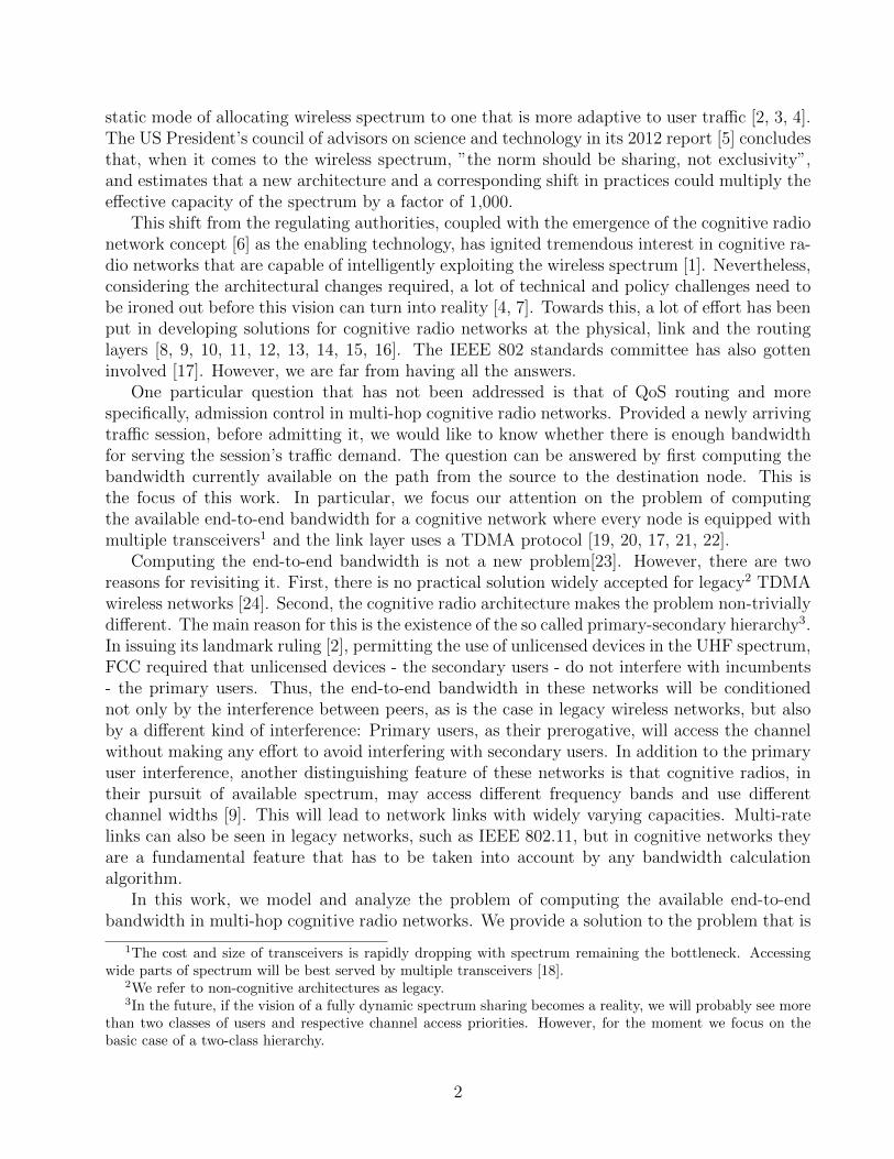
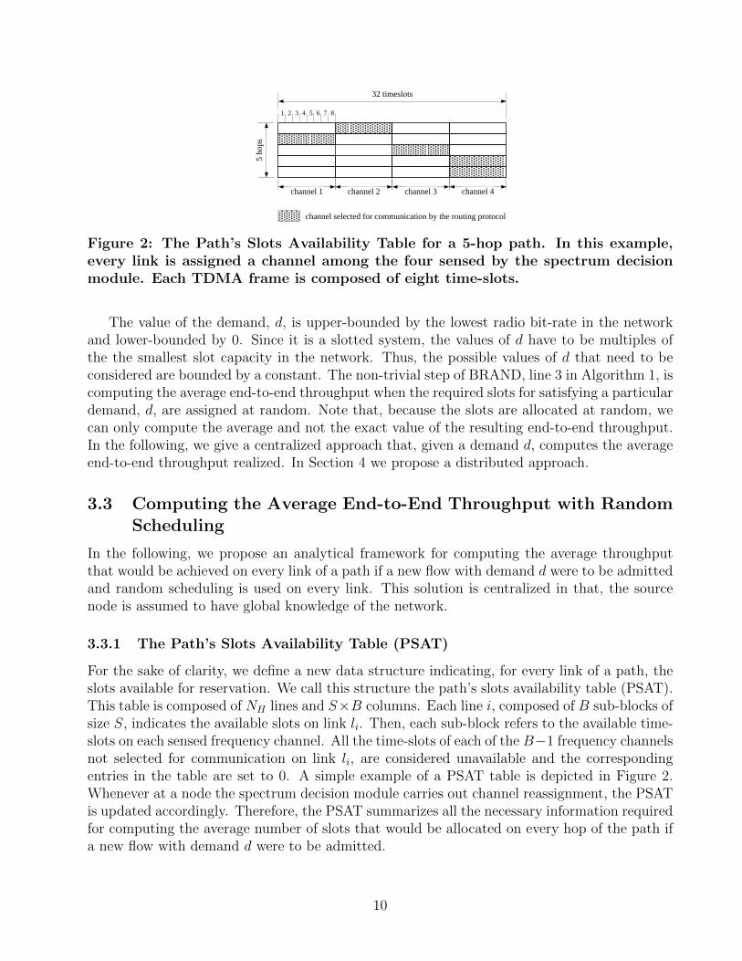
Figure 2: The Path’s Slots Availability Table for a 5-hop path. In this example,every link is assigned a channel among the four sensed by the spectrum decisionmodule. Each TDMA frame is composed of eight time-slots.
The value of the demand, d, is upper-bounded by the lowest radio bit-rate in the networkand lower-bounded by 0. Since it is a slotted system, the values of d have to be multiples ofthe the smallest slot capacity in the network. Thus, the possible values of d that need to beconsidered are bounded by a constant. The non-trivial step of BRAND, line 3 in Algorithm 1, iscomputing the average end-to-end throughput when the required slots for satisfying a particulardemand, d, are assigned at random. Note that, because the slots are allocated at random, wecan only compute the average and not the exact value of the resulting end-to-end throughput.In the following, we give a centralized approach that, given a demand d, computes the averageend-to-end throughput realized. In Section 4 we propose a distributed approach.
3.3 Computing the Average End-to-End Throughput with RandomScheduling
In the following, we propose an analytical framework for computing the average throughputthat would be achieved on every link of a path if a new flow with demand d were to be admittedand random scheduling is used on every link. This solution is centralized in that, the sourcenode is assumed to have global knowledge of the network.
3.3.1 The Path’s Slots Availability Table (PSAT)
For the sake of clarity, we define a new data structure indicating, for every link of a path, theslots available for reservation. We call this structure the path’s slots availability table (PSAT).This table is composed of NH lines and S×B columns. Each line i, composed of B sub-blocks ofsize S, indicates the available slots on link li. Then, each sub-block refers to the available time-slots on each sensed frequency channel. All the time-slots of each of the B−1 frequency channelsnot selected for communication on link li, are considered unavailable and the correspondingentries in the table are set to 0. A simple example of a PSAT table is depicted in Figure 2.Whenever at a node the spectrum decision module carries out channel reassignment, the PSATis updated accordingly. Therefore, the PSAT summarizes all the necessary information requiredfor computing the average number of slots that would be allocated on every hop of the path ifa new flow with demand d were to be admitted.
10
3.3.2 Fundamental principles of the method
To make the problem tractable, we relax it by working on average values. Even though math-ematically speaking E[a3] 6= min
(E[r3],E[A
(3)3 ]), we do such an approximation of the average
number of slots allocated on the third hop to reduce the calculation complexity. As depictedin section 5, our simulation results show that this approximation does not degrade the perfor-mance of the overall estimation process. Based on this assumption, a first solution consists ofestimating for each hop i the quantity A
(i)i which is now considered an average for the remaining
of the paper.l-link available slot set decomposition: From the PSAT, we can calculate for any
communication link li the set S(1)i containing the index of slots available for reservation on
that link at the beginning of the estimation process. The indexes of slots are now taken inthe set {1, 2, .., S.B} related to the super-frame composing the whole line in the PSAT. It isalso crucial to see that, when considering such an indexation, when a slot is allocated on li,it cannot be allocated anymore on both li+1 and li+2 as this would create interference. Thus,when this slot is only available for reservation on link li and neither on links li+1 nor li+2, the
sets S(j)i+1 and S
(j)i+2 are not impacted. Inversely, if this slot is also available to one of these links,
the corresponding sets are impacted and thus the number of slots that would be allocated onthe next hops is likely to decrease. Thus, each slot belongs to a certain category depending onthe links it appears to be available for reservation to. Therefore, we propose to divide the set{1, ..., S.B} in non overlapping subsets that cover {1, ..., S.B} and permit to categorise everyslot according to the links it is available for reservation to in the PSAT table. To be moreprecise, we define such a decomposition on a set of l consecutive links {i, i+ 1, ..., i+ l − 1}along the path. For k ∈ {0, 1, ..., l}, the number of subsets characterizing the slots available
to a set of k links but not the l − k others is(lk
). Thus, the total number of subsets in the
decomposition is∑lk=0
(lk
)= 2l. We refer to such a decomposition as a l-link available slot
set decomposition and use the following notations E(j)
a,b,cto denote the set of slots available for
reservation on both two links a and c but not b just before node nj does its allocations. Its
cardinality is written as C(j)
a,b,c.
To elucidate the meaning of these variables, let us consider a 3-hop path with the firstchannel selected for communication on every hop, B = 2, S = 8 and S
(1)1 = {2, 3, 4, 5},
S(1)2 = {2, 6, 7} and S
(1)3 = {1, 2, 4, 5, 6, 7}. This leads to the following eigth sets: E
(1)1,2,3 = {2},
E(1)
1,2,3= ∅, E(1)
1,2,3= {4, 5}, E(1)
1,2,3= {6, 7}, E(1)
1,2,3= {3}, E(1)
1,2,3= ∅, E(1)
1,2,3= {1} and E
(1)
1,2,3=
{8, 9, ..., 16}.Achievable end-to-end throughput calculation: The random nature of the slot allo-
cation process provides good properties to evaluate the average number of slots impacted inevery subset as further depicted for the case of a 3-hop path for which a flow with demand dneeds to be relayed from the source to the destination. From now on, we work with averagevalues. From the PSAT, we can compute the 3-link available slot set decomposition related tol1, l2 and l3. At the same time, the initial number of available slots on every communicationlink A
(1)i can be calculated. To forward the new traffic flow to its next hop n2, node n1 reserves
exactly a1 = min (r1, A(1)1 ) additional slots on the first communication link. Among these slots,
some might have also been available for reservation on links l2 and l3 but, due to interference,
11
become unavailable after these allocations.Let us consider a discrete random variable Xi taking its values in the set {0, 1, ..., ai} and
representing the number of slots initially available for reservation on link li that have beenreserved by node n1 to relay the new incoming flow on l1. Xi represents the number of slotsin the set S
(1)1 ∩ S
(1)i reserved by n1 for communication on l1. Intuitively, as the slots are
allocated at random, we see that a proportion a1/A(1)1 of these slots are likely to be reserved
by n1. Mathematically speaking, Xi follows an hypergeometric distribution with parameters(A
(1)1 , |S(1)
1 ∩ S(1)i |, a1). The expectation value of such a random variable is E[Xi] = |S(1)
1 ∩S(1)i | × a1/A
(1)1 and thus, in every set S
(1)1 ∩ S
(1)i , an average proportion p1 = a1/A
(1)1 of slots is
reserved by node n1. Note that for the case of A(1)1 = 0 we get a1 = 0 and p1 = 0. Exactly
the same analysis can be carried out on every set resulting from the 3-link available slot setdecomposition related to l1, l2 and l3. This way, the average values A
(2)2 and A
(2)3 just after n1
did its reservations can be computed as detailed in Algorithm 2 and illustrated in Figure 3.Therefore, the average number of slots allocated on the following links can be evaluated andthe process repeated until the average number of slots allocated on the last hop is calculated.
𝐸1 ,2
𝐸1 ,2
𝐸1,2
𝐸1,2 (1)
(1) (1)
(1)
{1, … , 𝑆 × 𝐵}
𝐸1 ,2, 3
𝐸1 ,2,3
𝐸1,2 ,3 (1)
(1)
(1)
{1, … , 𝑆 × 𝐵}
𝐸1 ,2, 3 (1)
𝐸1,2 ,3 (1)
𝐸1,2,3 (1)
𝐸1 ,2,3 (1)
𝐸1,2,3 (1)
(a) 2-link available slot set decomposition
𝐸1 ,2
𝐸1 ,2
𝐸1,2
𝐸1,2 (1)
(1) (1)
(1)
{1, … , 𝑆 × 𝐵}
𝐸1 ,2, 3
𝐸1 ,2,3
𝐸1,2 ,3 (1)
(1)
(1)
{1, … , 𝑆 × 𝐵}
𝐸1 ,2, 3 (1)
𝐸1,2 ,3 (1)
𝐸1,2,3 (1)
𝐸1 ,2,3 (1)
𝐸1,2,3 (1)
(b) 3-link available slot set decomposition
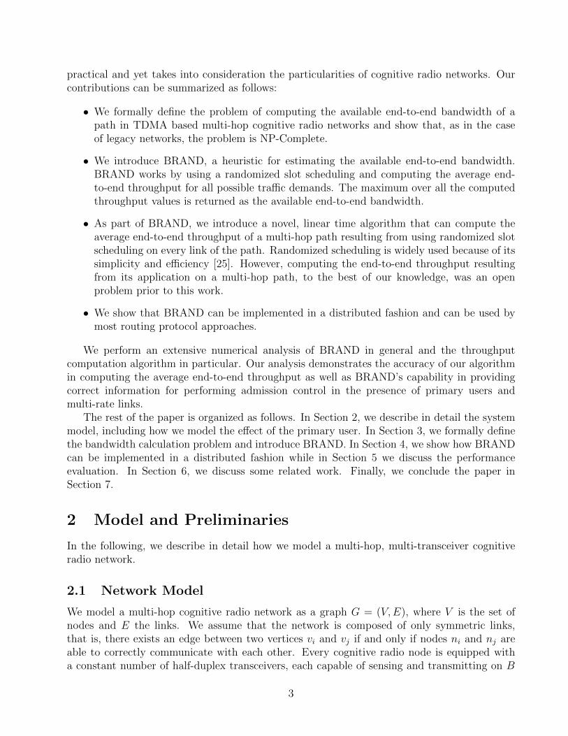
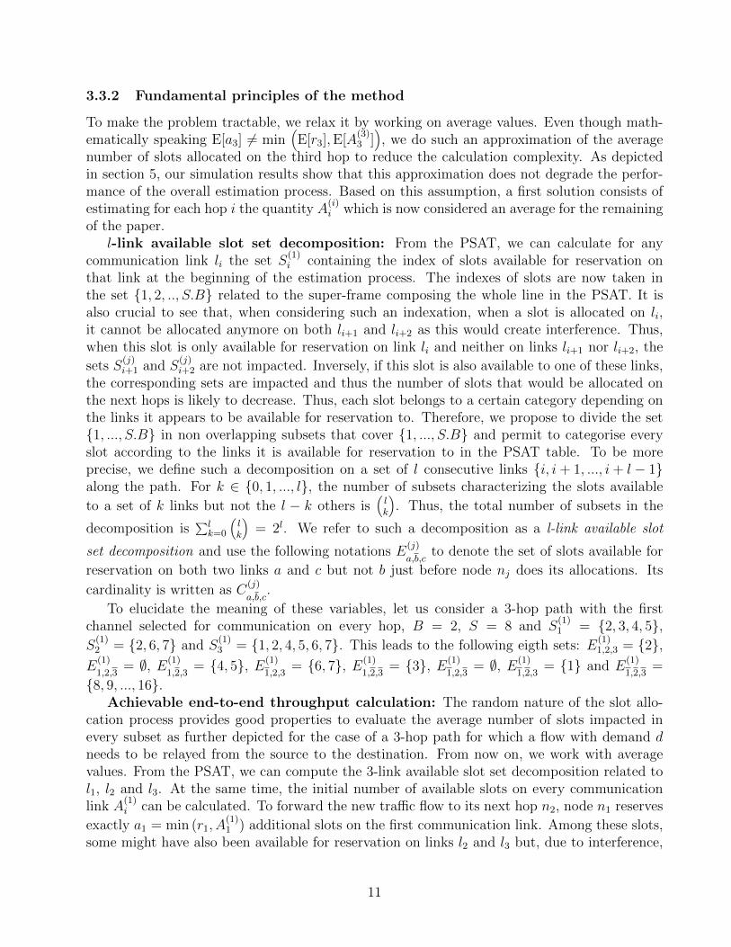
Figure 3: When slot allocations are carried out on l1 the proportion of slots allo-cated, p1, is removed from every subset that characterizes slots initially availablefor reservation on l1, E
(1)1,2,3. This proportion is represented by plain areas in the
above figures. The selected slots become unavailable on all three links and thus aretransferred to the set of unavailable slots for those links. The same mechanism isthen repeated for the allocations carried out on l2. This time, the slots are selectedat random among those remaining available for reservations. The proportion ofslots selected, p2, represented by dotted areas, is thus taken in every subset char-acterizing slots remaining available for allocation on l2, E
(2)1,2,3. Finally, the same
mechanism is in place for allocations on link l3, as depicted by the striped areas.
This approach still applies when increasing the path length. However, the impact of n1
allocations is still required to be evaluated when computing the average number of slots thatwould be allocated on any further communication link li. Such an impact can be evaluatedby first doing the i-link available slot set decomposition and then carefully measuring thedependence of each of the previous node allocations. This leads to an exponential number of
12
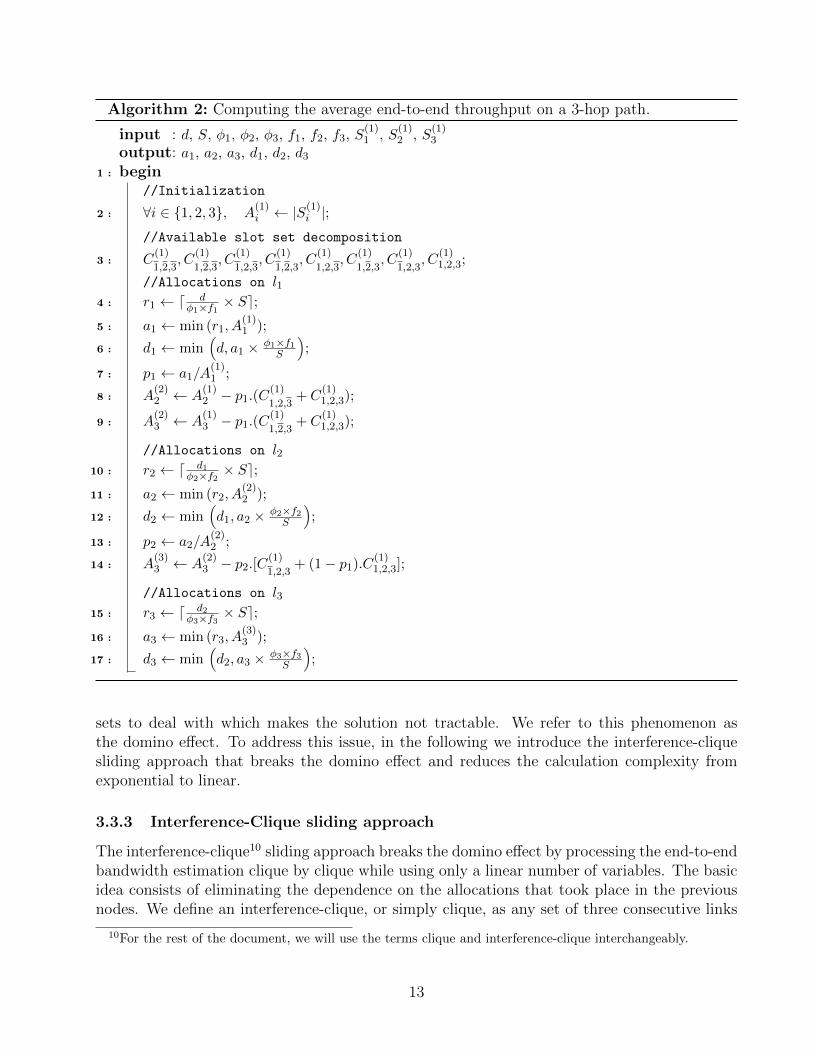
Algorithm 2: Computing the average end-to-end throughput on a 3-hop path.
input : d, S, φ1, φ2, φ3, f1, f2, f3, S(1)1 , S
(1)2 , S
(1)3
output: a1, a2, a3, d1, d2, d31 : begin
//Initialization
2 : ∀i ∈ {1, 2, 3}, A(1)i ← |S
(1)i |;
//Available slot set decomposition
3 : C(1)
1,2,3, C
(1)
1,2,3, C
(1)
1,2,3, C
(1)
1,2,3, C
(1)
1,2,3, C
(1)
1,2,3, C
(1)
1,2,3, C
(1)1,2,3;
//Allocations on l14 : r1 ← d d
φ1×f1 × Se;5 : a1 ← min (r1, A
(1)1 );
6 : d1 ← min(d, a1 × φ1×f1
S
);
7 : p1 ← a1/A(1)1 ;
8 : A(2)2 ← A
(1)2 − p1.(C
(1)
1,2,3+ C
(1)1,2,3);
9 : A(2)3 ← A
(1)3 − p1.(C
(1)
1,2,3+ C
(1)1,2,3);
//Allocations on l210 : r2 ← d d1
φ2×f2 × Se;11 : a2 ← min (r2, A
(2)2 );
12 : d2 ← min(d1, a2 × φ2×f2
S
);
13 : p2 ← a2/A(2)2 ;
14 : A(3)3 ← A
(2)3 − p2.[C
(1)
1,2,3+ (1− p1).C(1)
1,2,3];
//Allocations on l315 : r3 ← d d2
φ3×f3 × Se;16 : a3 ← min (r3, A
(3)3 );
17 : d3 ← min(d2, a3 × φ3×f3
S
);
sets to deal with which makes the solution not tractable. We refer to this phenomenon asthe domino effect. To address this issue, in the following we introduce the interference-cliquesliding approach that breaks the domino effect and reduces the calculation complexity fromexponential to linear.
3.3.3 Interference-Clique sliding approach
The interference-clique10 sliding approach breaks the domino effect by processing the end-to-endbandwidth estimation clique by clique while using only a linear number of variables. The basicidea consists of eliminating the dependence on the allocations that took place in the previousnodes. We define an interference-clique, or simply clique, as any set of three consecutive links
10For the rest of the document, we will use the terms clique and interference-clique interchangeably.
13
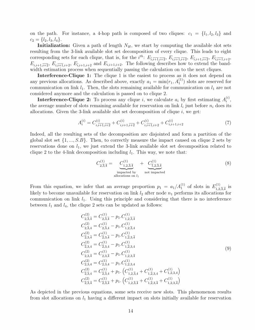
on the path. For instance, a 4-hop path is composed of two cliques: c1 = {l1, l2, l3} andc2 = {l2, l3, l4}.
Initialization: Given a path of length NH , we start by computing the available slot setsresulting from the 3-link available slot set decomposition of every clique. This leads to eightcorresponding sets for each clique, that is, for the ith: Ei,i+1,i+2, Ei,i+1,i+2, Ei,i+1,i+2, Ei,i+1,i+2,Ei,i+1,i+2, Ei,i+1,i+2, Ei,i+1,i+2 and Ei,i+1,i+2. The following describes how to extend the band-width estimation process when sequentially passing the calculation on to the next cliques.
Interference-Clique 1: The clique 1 is the easiest to process as it does not depend onany previous allocations. As described above, exactly a1 = min(r1, A
(1)1 ) slots are reserved for
communication on link l1. Then, the slots remaining available for communication on l1 are notconsidered anymore and the calculation is passed on to clique 2.
Interference-Clique 2: To process any clique i, we calculate ai by first estimating A(i)i ,
the average number of slots remaining available for reservation on link li just before ni does itsallocations. Given the 3-link available slot set decomposition of clique i, we get:
A(i)i = C
(i)
i,i+1,i+2+ C
(i)
i,i+1,i+2+ C
(i)
i,i+1,i+2+ C
(i)i,i+1,i+2 (7)
Indeed, all the resulting sets of the decomposition are disjointed and form a partition of theglobal slot set {1, ..., S.B}. Then, to correctly measure the impact caused on clique 2 sets byreservations done on l1, we just extend the 3-link available slot set decomposition related toclique 2 to the 4-link decomposition including l1. This way, we note that:
C(1)
2,3,4= C
(1)
1,2,3,4︸ ︷︷ ︸impacted by
allocations on l1
+ C(1)
1,2,3,4︸ ︷︷ ︸not impacted
(8)
From this equation, we infer that an average proportion p1 = a1/A(1)1 of slots in E
(1)
1,2,3,4is
likely to become unavailable for reservation on link l2 after node n1 performs its allocations forcommunication on link l1. Using this principle and considering that there is no interferencebetween l1 and l4, the clique 2 sets can be updated as follows:
C(2)
2,3,4= C
(1)
2,3,4− p1.C(1)
1,2,3,4
C(2)
2,3,4= C
(1)
2,3,4− p1.C(1)
1,2,3,4
C(2)
2,3,4= C
(1)
2,3,4− p1.C(1)
1,2,3,4
C(2)
2,3,4= C
(1)
2,3,4− p1.C(1)
1,2,3,4
C(2)
2,3,4= C
(1)
2,3,4− p1.C(1)
1,2,3,4
C(2)2,3,4 = C
(1)2,3,4 − p1.C
(1)1,2,3,4
C(2)
2,3,4= C
(1)
2,3,4+ p1.
(C
(1)
1,2,3,4+ C
(1)
1,2,3,4+ C
(1)1,2,3,4
)C
(2)
2,3,4= C
(1)
2,3,4+ p1.
(C
(1)
1,2,3,4+ C
(1)
1,2,3,4+ C
(1)
1,2,3,4
)
(9)
As depicted in the previous equations, some sets receive new slots. This phenomenon resultsfrom slot allocations on l1 having a different impact on slots initially available for reservation
14
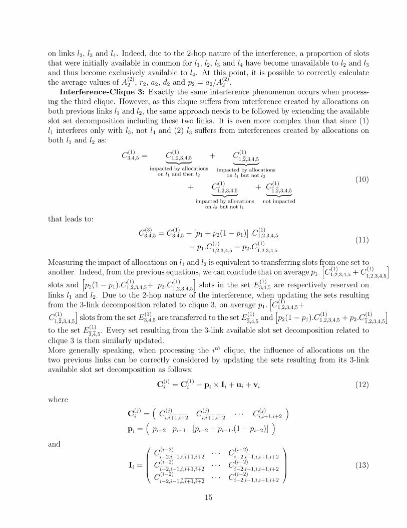
on links l2, l3 and l4. Indeed, due to the 2-hop nature of the interference, a proportion of slotsthat were initially available in common for l1, l2, l3 and l4 have become unavailable to l2 and l3and thus become exclusively available to l4. At this point, it is possible to correctly calculatethe average values of A
(2)2 , r2, a2, d2 and p2 = a2/A
(2)2 .
Interference-Clique 3: Exactly the same interference phenomenon occurs when process-ing the third clique. However, as this clique suffers from interference created by allocations onboth previous links l1 and l2, the same approach needs to be followed by extending the availableslot set decomposition including these two links. It is even more complex than that since (1)l1 interferes only with l3, not l4 and (2) l3 suffers from interferences created by allocations onboth l1 and l2 as:
C(1)3,4,5 = C
(1)1,2,3,4,5︸ ︷︷ ︸
impacted by allocationson l1 and then l2
+ C(1)
1,2,3,4,5︸ ︷︷ ︸impacted by allocations
on l1 but not l2
+ C(1)
1,2,3,4,5︸ ︷︷ ︸impacted by allocations
on l2 but not l1
+ C(1)
1,2,3,4,5︸ ︷︷ ︸not impacted
(10)
that leads to:
C(3)3,4,5 = C
(1)3,4,5 − [p1 + p2(1− p1)] .C(1)
1,2,3,4,5
− p1.C(1)
1,2,3,4,5− p2.C(1)
1,2,3,4,5
(11)
Measuring the impact of allocations on l1 and l2 is equivalent to transferring slots from one set toanother. Indeed, from the previous equations, we can conclude that on average p1.
[C
(1)1,2,3,4,5 + C
(1)
1,2,3,4,5
]slots and
[p2(1− p1).C(1)
1,2,3,4,5+ p2.C(1)
1,2,3,4,5
]slots in the set E
(1)3,4,5 are respectively reserved on
links l1 and l2. Due to the 2-hop nature of the interference, when updating the sets resultingfrom the 3-link decomposition related to clique 3, on average p1.
[C
(1)1,2,3,4,5+
C(1)
1,2,3,4,5
]slots from the setE
(1)3,4,5 are transferred to the set E
(1)
3,4,5and
[p2(1− p1).C(1)
1,2,3,4,5 + p2.C(1)
1,2,3,4,5
]to the set E
(1)
3,4,5. Every set resulting from the 3-link available slot set decomposition related to
clique 3 is then similarly updated.More generally speaking, when processing the ith clique, the influence of allocations on thetwo previous links can be correctly considered by updating the sets resulting from its 3-linkavailable slot set decomposition as follows:
C(i)i = C
(1)i − pi × Ii + ui + vi (12)
where
C(j)i =
(C
(j)
i,i+1,i+2C
(j)
i,i+1,i+2· · · C
(j)i,i+1,i+2
)pi =
(pi−2 pi−1 [pi−2 + pi−1.(1− pi−2)]
)and
Ii =
C
(i−2)i−2,i−1,i,i+1,i+2
· · · C(i−2)i−2,i−1,i,i+1,i+2
C(i−2)i−2,i−1,i,i+1,i+2
· · · C(i−2)i−2,i−1,i,i+1,i+2
C(i−2)i−2,i−1,i,i+1,i+2
· · · C(i−2)i−2,i−1,i,i+1,i+2
(13)
15

The vector ui serves to compensate a set that does not suffer from all of the interferences. Thevector vi is then used to update the sets receiving slots becoming unavailable for reservationon certain links. The values of vectors ui and vi depend on some variables used in pi and Iiand are given in the Appendix.Once the clique sets are updated, the average values A
(i)i , ri, ai, di and pi = ai/A
(i)i can be
correctly evaluated and the calculation process can be passed on to the following clique.Interference-Clique 4 and beyond: When processing the third clique, the entries of
matrix Ii were strictly referring to sets that had not varied from the beginning of the estima-tion process. However, that is not the case when processing the fourth clique. Indeed, thecorresponding sets are likely to have been impacted by allocations on previous links. Such aset, for instance E
(2)
2,3,4,5,6, has suffered from allocations on l1 and thus needs also to be updated.
A straight solution would consist in forming the sets resulting from the 6-link available slot setdecomposition and identify the way every set is impacted. This method is correct but leadsto the previously mentioned domino effect. Fortunately, the random nature of the slot alloca-tion can simplify the analysis and bound the number of variables to deal with for each cliqueprocess. In the following, we illustrate this point when processing any clique i ≥ 4. We nowshow how to characterize a set used in the clique i set update equation, say E
(i−2)i−2,i−1,i,i+1,i+2
, as
a function of its initial state. We start by doing the 2-link available slot set decomposition re-lated to li−2 and li−1. This decomposition leads to four disjointed sets: E
(j)
i−2,i−1,E(j)
i−2,i−1,E(j)
i−2,i−1
and E(j)i−2,i−1. Let us work on the third one, that is E
(j)
i−2,i−1. This set can also be divided in
eight disjointed subsets resulting from the 3-link available slot set decomposition of clique i.This time, the slot space equals E
(j)
i−2,i−1 rather than {1, 2, ..., S.B}, leading to subsets of the
following form E(j)
i−2,i−1,i,i+1,i+2, taken as an example. A property of the set E
(j)
i−2,i−1 is that
along the estimation process, it can only transfer slots to the set E(j)
i−2,i−1 and cannot receive
slots from another. Therefore, the number of slots that initially belonged to the set E(j)
i−2,i−1and had become unavailable just before node ni−2 did its reservations for communication on
link li−2 equals C(1)
i−2,i−1 − C(i−2)i−2,i−1. These slots had become unavailable due to allocations on
li−4 and li−3. Because of the random nature of the slot reservation process, these slots were
taken uniformly at random among the subsets partitioning E(j)
i−2,i−1. We can thus represent the
number of slots that had become unavailable in the set E(j)
i−2,i−1,i,i+1,i+2with the discrete ran-
dom variable Xi−2,i−1,i,i+1,i+2 taking its values in the set {0, ..., C(1)
i−2,i−1−C(i−2)i−2,i−1} and following
an hypergeometric distribution with parameters (C(1)
i−2,i−1, C(1)
i−2,i−1,i,i+1,i+2, C
(1)
i−2,i−1 − C(i−2)i−2,i−1).
From this identification we can deduce that, for C(1)
i−2,i−1 strictly positive, the average value of
this random variable equals [(C(1)
i−2,i−1 − C(i−2)i−2,i−1)/C
(1)
i−2,i−1]× C(1)
i−2,i−1,i,i+1,i+2.
More generally, just before node ni−2 did its allocations, an average proportion C(i−2)i−2,i−1/C
(1)
i−2,i−1
of the initially available slots remained available in every subset partitioning E(j)
i−2,i−1. Hereafter,
the quantity C(i−2)i−2,i−1,i,i+1,i+2
can be correctly evaluated as follows:
C(i−2)i−2,i−1,i,i+1,i+2
= C(1)
i−2,i−1,i,i+1,i+2× αi−2,i−1 (14)
16
where the reduction factor of the set E(j)
i−2,i−1 equals
αi−2,i−1 =
0 , if C
(1)
i−2,i−1 = 0
C(i−2)
i−2,i−1
C(1)
i−2,i−1
=C
(i−2)
i−2,i−1,i+C
(i−2)
i−2,i−1,i
C(1)
i−2,i−1,i+C
(1)
i−2,i−1,i
, else(15)
and is related to clique (i − 2) as it can be computed at the beginning of the process of this
clique. The same analysis can be carried out for the two other sets of interest E(j)
i−2,i−1 and
E(j)i−2,i−1. However, it differs a little for E
(j)
i−2,i−1 when C(1)
i−2,i−1 = 0 as this set can receive
slots from E(j)i−2,i−1 due to allocations on previous links. For this case, to correctly update the
resulting subsets, we compute the proportion of slots transferred from E(j)i−2,i−1 to E
(j)
i−2,i−1. The
quantity C(i−2)i−2,i−1,i,i+1,i+2
can be correctly evaluated as follows:
C(i−2)i−2,i−1,i,i+1,i+2
= C(1)i−2,i−1,i,i+1,i+2 × τi−2 (16)
with
τi−2 =C
(i−2)i−2,i−1
C(1)i−2,i−1
=C
(i−2)i−2,i−1,i + C
(i−2)i−2,i−1,i
C(1)
i−2,i−1,i + C(1)i−2,i−1,i
(17)
if C(1)i−2,i−1 is strictly positive, and zero otherwise.Then, no additional techniques are required to process the remaining cliques and the calcu-
lation can be completed by simply applying the approach given in algorithm 2 when processingthe last clique of the path. The main advantage of this approach is that there is no dominoeffect and the resulting calculation complexity is O(NH).
4 Distributed Implementation of BRAND
In Section 3 we presented a centralized version of BRAND. This version can be easily appliedwith source routing protocols, like DSR [33], where the path computation is centralized at thesource. However, this is not the case for non-source routing protocols, like the popular OLSR[34], where the route computation is performed in a distributed fashion by every node. Toaddress this limitation of the centralized version we present a simple mechanism that enables thedistributed execution of BRAND. The proposed mechanism makes possible the implementationof BRAND with any routing protocols, regardless of how they perform path computations.
BRAND estimates the available end-to-end bandwidth by estimating, for all possible de-mands, the average end-to-end throughput of a given path and returning the maximum suchvalue. Next, we describe a distributed implementation of the throughput computation and inSection 4.2 we describe how this process can be repeated for all possible demands.
4.1 Distributed Computation of the Average End-to-End Through-put
As described in Section 3, applying the interference-clique sliding technique for computing theaverage throughput of a given path given a demand, d, requires the knowledge of the interference
17

clique. In a distributed setting, this requirement means that every node executing the algorithmwill need to know the next three hops on the particular path. Unfortunately, with protocolslike OLSR [34] or AODV [35], nodes only store the next-hop for a given source-destinationpair. To overcome this challenge, we propose a simple trick: Simply shift the interference-clique calculation two hops down the path. Doing so will require, for example, node n3 todo the computation related to the first interference clique, consisting of l1, l2, l3, that normallywould be done by n1. Regardless of the routing protocol, node n3 will know n1, n2 and n4 and,therefore, will have the necessary information to execute our algorithm.
The source node starts by sending a bandwidth calculation init packet to its next hop. Thispacket contains the destination node id, necessary information for performing the calculationfor the first link (initial demand d, φ1, f1) and a flow id used to identify the session for whichthe calculation is carried out. Node n2 uses the destination id to identify the next hop, node n3,and transfer the bandwidth calculation init packet to n3 with additional necessary informationfor doing the calculation for the first clique (φ2, f2). Node n3 is then capable of identifying thenext hop n4 and does the computation related to the first interference-clique, l1, l2, l3. Oncethis computation is done, n3 sends a bandwidth calculation request packet to its next hop, n4.This packet contains the destination node id, the flow id, d1, φ2, φ3, f2, f3, p1 and S
(1)1
11.This way, n4 has sufficient information to do the computation for the second clique, l2, l3, l4.Once this computation is done, n4 follows the same procedure as n3 and sends a bandwidthcalculation request packet to its next hop. This packet contains the destination node id, theflow id, d2, φ3,φ4, f3,f4, p1, p2, S
(1)1 , S
(1)2 and the three reduction factors related to clique 2 with
possibly τ2 that will serve in the computation for the fourth clique. With receiving this packet,n5 can do the computation related to the third clique. Then, it sends a bandwidth calculationrequest packet to its next hop on the path. This packet contains the destination node id, theflow id, d3, φ4, φ5, f4, f5, p2, p3, S
(1)2 , S
(1)3 the three reduction factors related to clique 2 with
possibly τ2 and the three reduction factors related to clique 3 with possibly τ3. Thus, n6 hassufficient information to do the calculation related to clique 4.
This same process is repeated till reaching the last node before the destination, as doing thecalculations for the following cliques requires no additional fields in the bandwidth calculationrequest packet. When the last node before the destination receives a bandwidth request packet,it knows it is processing the calculation for the last clique. Using the information receivedin the packet it updates the last clique sets’ information and applies the method provided inAlgorithm 2 to compute the average end-to-end throughput. Once it finishes the calculation itsends a bandwidth calculation response packet back to the source with the resulting throughputvalue.
4.2 Looping over All Possible Demands
BRAND requires estimating the average end-to-end throughput for all possible demands. Thiscan be done in two ways. One approach is for the source to initiate multiple bandwidthcalculation procedures, one for every demand d taken in the range [0,min (φ1, φ2)] with step∆φ. The step ∆φ can be selected by the source node and can be as simple as the smallestcapacity it can allocate. Another approach is to do the calculation for all such demands at
11Every node is assumed to have 2-hop slot availability information.
18
once, at every hop, and then encapsulate the corresponding data related to each demand in theresulting request packets. In this case the size of the bandwidth calculation request packet isbigger but the end-to-end process is carried out once.
In terms of computation complexity, the number of operations for processing a clique isconstant. Therefore, for every demand, the resulting complexity is O(NH). If the backwardpath of the response packet from the last node before the destination to the source is similarto the forwarding path of requests packets, the round trip time for the average end-to-endthroughput calculation is bounded by 2T×(NH−1) with T equal to the TDMA frame duration.
5 Performance evaluation of Brand
In this section, we evaluate BRAND numerically using MATLAB and compare it with the workof Zhu et al. [23]. In summary, we make the following main observations:
• In Section 5.2, we demonstrate that although BRAND uses a very simple schedulingheuristic –randomized scheduling – its achieved end-to-end bandwidth is competitive whencompared with the optimal policy.
• In Section 5.3, we demonstrate the correctness of BRAND’s algorithm for computing theaverage throughput of randomized scheduling.
• In Section 5.4, we demonstrate that BRAND delivers the bandwidth it promises in achiev-ing an almost perfect admission control.
• In Section 5.5, we demonstrate that BRAND deals successfully with the challenges arisingfrom the cognitive radio network architecture. Specifically, BRAND maintains an almostperfect admission control in face of Primary User interference and multi-rate links.
• Also in Section 5.5, in comparing with a heuristic not designed for cognitive radio net-works, we demonstrate the significant effect multi-rate links and the Primary User in-terference can have on the available end-to-end bandwidth and ultimately, the admissioncontrol.
5.1 Simulation Parameters
Each link is assigned one orthogonal channel among four sensed ones. The medium is accessedthrough a TDMA MAC with 40 slots per frame. As the specific spectrum assignment processis beyond the scope of this paper, we simply use the following probabilistic model to selectthe assigned channel for each communication link: P[channel1] = 0.80, P[channel2] = 0.10,P[channel3] = 0.05 and P[channel4] = 0.05. The probabilities are purposely selected to achievea high self-interference on the path and thus, to show the worst-case performance of the algo-rithm. The scheduling algorithm in the simulation is the same with the one used by BRAND,i.e., the necessary allocations of slots are performed at random among those available.
In practice, link rates depend on the local environment and may fluctuate with time. Toapproximate this behavior, we sample every link rate φi according to a normal distributionwith mean µφ and standard deviation σφ where µφ is the mean link transmission rate on the
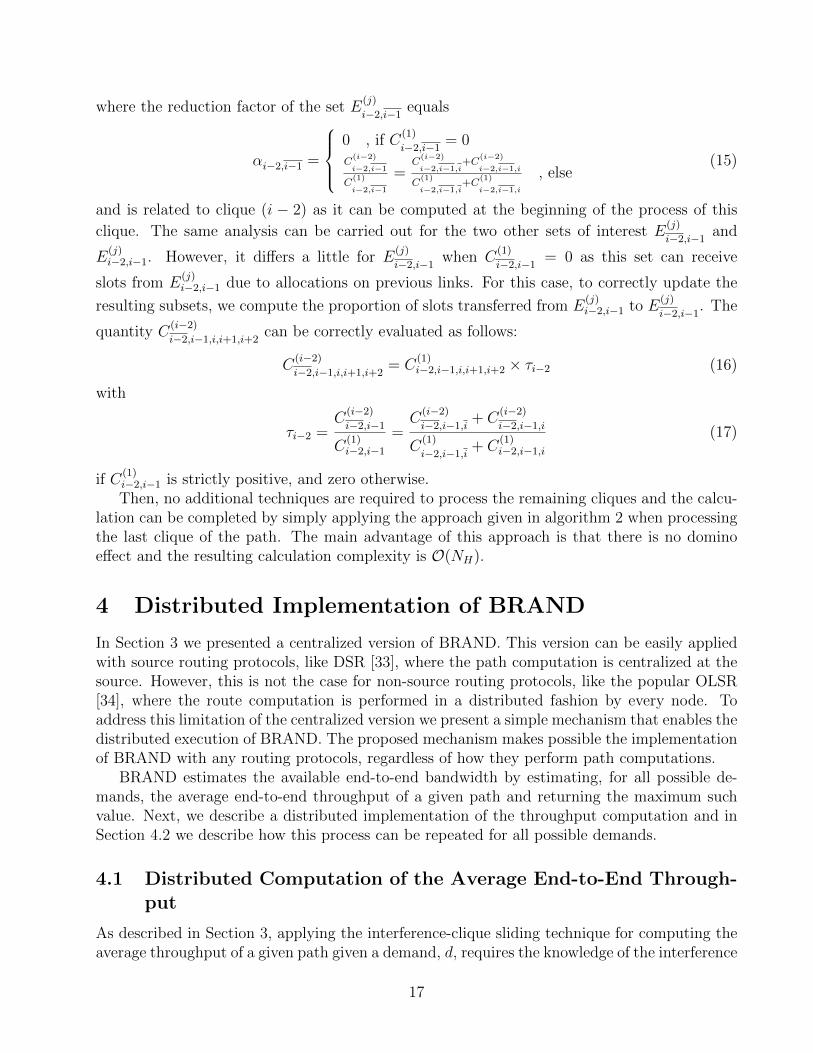
19
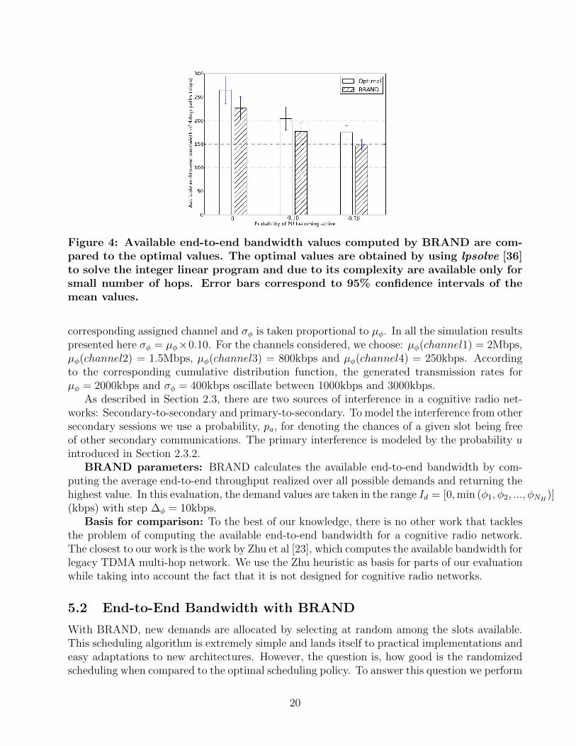
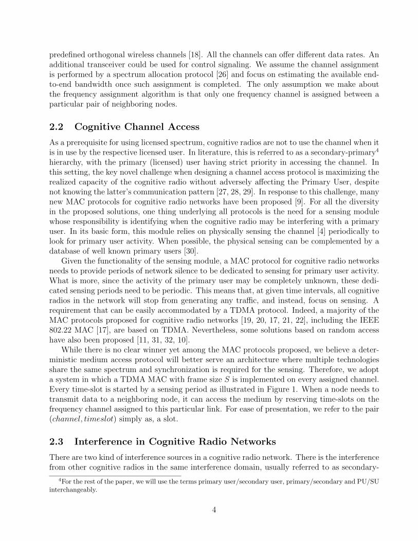
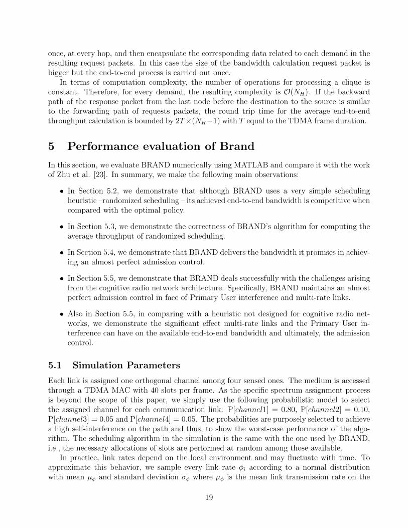
Figure 4: Available end-to-end bandwidth values computed by BRAND are com-pared to the optimal values. The optimal values are obtained by using lpsolve [36]to solve the integer linear program and due to its complexity are available only forsmall number of hops. Error bars correspond to 95% confidence intervals of themean values.
corresponding assigned channel and σφ is taken proportional to µφ. In all the simulation resultspresented here σφ = µφ×0.10. For the channels considered, we choose: µφ(channel1) = 2Mbps,µφ(channel2) = 1.5Mbps, µφ(channel3) = 800kbps and µφ(channel4) = 250kbps. Accordingto the corresponding cumulative distribution function, the generated transmission rates forµφ = 2000kbps and σφ = 400kbps oscillate between 1000kbps and 3000kbps.
As described in Section 2.3, there are two sources of interference in a cognitive radio net-works: Secondary-to-secondary and primary-to-secondary. To model the interference from othersecondary sessions we use a probability, pa, for denoting the chances of a given slot being freeof other secondary communications. The primary interference is modeled by the probability uintroduced in Section 2.3.2.
BRAND parameters: BRAND calculates the available end-to-end bandwidth by com-puting the average end-to-end throughput realized over all possible demands and returning thehighest value. In this evaluation, the demand values are taken in the range Id = [0,min (φ1, φ2, ..., φNH
)](kbps) with step ∆φ = 10kbps.
Basis for comparison: To the best of our knowledge, there is no other work that tacklesthe problem of computing the available end-to-end bandwidth for a cognitive radio network.The closest to our work is the work by Zhu et al [23], which computes the available bandwidth forlegacy TDMA multi-hop network. We use the Zhu heuristic as basis for parts of our evaluationwhile taking into account the fact that it is not designed for cognitive radio networks.
5.2 End-to-End Bandwidth with BRAND
With BRAND, new demands are allocated by selecting at random among the slots available.This scheduling algorithm is extremely simple and lands itself to practical implementations andeasy adaptations to new architectures. However, the question is, how good is the randomizedscheduling when compared to the optimal scheduling policy. To answer this question we perform
20
0 50 100 150 200 250 300 350 400 450 5000
50
100
150
200
250
300
350
400
450
500
Computed end−to−end throughput (kbps)
Exa
ct e
nd−
to−
end
thro
ughp
ut o
btai
ned
by s
imul
atio
n (k
bps)
pa = 33%, NH = 4
pa = 50%, NH = 4
(a) Numerical verification for a 4-hop path.
0 50 100 150 200 250 300 350 400 450 5000
50
100
150
200
250
300
350
400
450
500
Computed end-to-end throughput (kbps)
Exa
cten
d−to
−en
dth
roug
hput
obta
ined
bysi
mul
atio
n(k
bps)
pa = 33%, NH = 10
pa = 50%, NH = 10
(b) Numerical verification for a 10-hop path.
Figure 5: Numerical verification of the correctness of the algorithm for computingthe average throughput introduced in Section 3.3. The y−axis represents the valuesobtained numerically, and for these graphs are averages over 5 runs. The proba-bility of PU interference is set to 10%. Even after only 5 numerical experiments,the average numerical values are quickly converging to the values computed by thealgorithm.
the following experiment. We choose the values of no secondary interference, pa, for every linkuniformly at random in (0, 1) and generate PSAT tables for various path sizes. We run BRANDin MATLAB using these PSAT tables and compute the available end-to-end bandwidth fordifferent values of primary user interference. Given that computing the optimal slot schedulingis NP-Complete, we formulate the problem as an integer linear program, see Appendix D, anduse lpsolve [36] to generate optimal scheduling assignments for a given PSAT table of a givenpath. The optimal schedules computed for the same PSAT tables as the ones used for BRANDare then fed into MATLAB for computing the resulting available end-to-end bandwidth. Asevident by the formulation shown in the Appendix D, the integer linear program gets highlycomplicated for high number of hops so we were able to compute optimal values for paths ofup to four hops.
Figure 4 shows the optimal values as well as the ones computed by BRAND for the availableend-to-end bandwidth of a 4-hop path as a function of primary user occurrence probability. Asthe data shows, BRAND is within 85% of the optimal policy despite using a very simplescheduling heuristic.
5.3 End-to-End Throughput with Randomized Scheduling
The most novel and challenging part of BRAND is its algorithm for computing the averagethroughput of randomized scheduling, introduced in Section 3.3. Given the involved analysis ofthe algorithm, here we perform a simple experiment for verifying its correctness. For a specificvalue of hop-count and pa we generate a PSAT table using MATLAB. The algorithm is appliedusing the PSAT table and the average end-to-end throughput is computed for all demands
21
0 100 200 300 400 500 6000
100
200
300
400
500
600
Available end−to−end bandwidth (kbps)
Adm
itted
rat
e in
pra
ctic
e (k
bps)
NH = 4, u = 10%
NH = 10, u = 10%
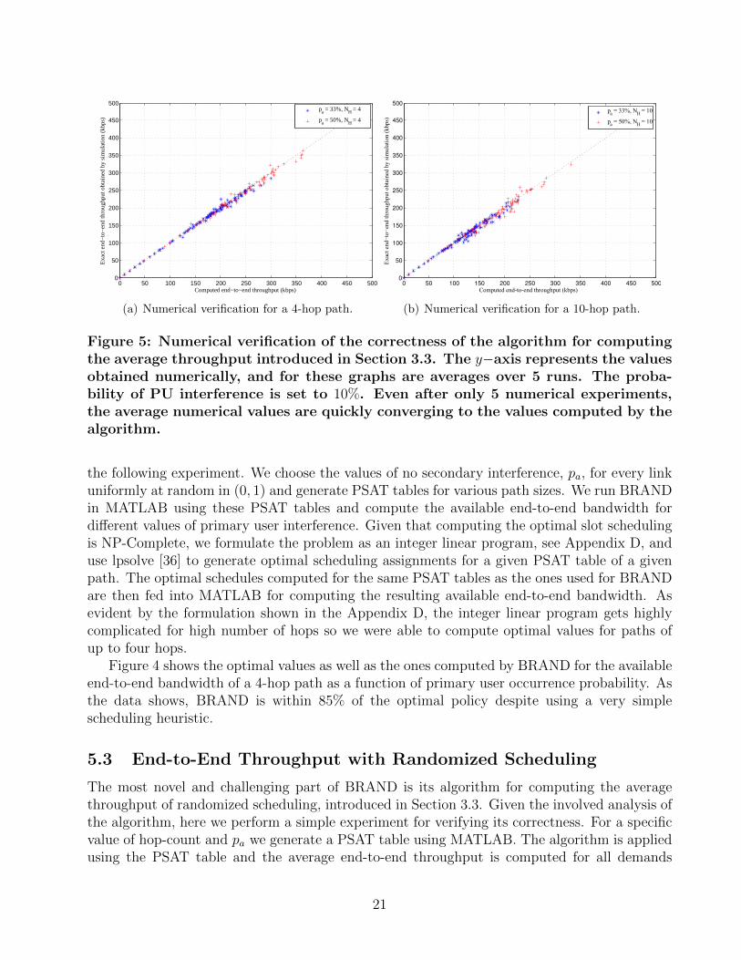
Figure 6: The x-axis represents the available end-to-end bandwidth computed byBRAND for various probabilities of no secondary interference. The y-axis rep-resents the end-to-end throughput measured in simulations – utilizing the samePSAT as the computation – when the traffic demand is equal to the respectiveend-to-end bandwidth computed by BRAND. The data shown here is for paths offour (NH = 4) and ten hops (NH = 10). Nearly 100% admission is achieved.
described in Section 5.1. With the same PSAT and traffic demands, we run simulations inMATLAB in which the slots are selected at random on every hop. The simulation is runmultiple times and the seed for the random generator is changed every time. The throughputvalues measured at the end of each simulation are averaged over all runs. In Figure 5, for everydemand, the computed and the measured throughput values for pa = 33% and pa = 50% areplotted on the x and y-axis, respectively. The probability of PU interference is set to 10%.The data shown are for path lengths of 4 hops, a reasonably sized multi-hop networks, and 10hops, a large network. After 5 runs the measurements are already converging to the computedvalues.
5.4 Admission Control Performance
BRAND is designed for enabling admission control. As such, we expect any flow with demandless than or equal to the available bandwidth computed by BRAND to be admitted end-to-end.To verify that this is the case, we perform the following two-step experiment. In the first step,we apply BRAND on a 4-hop path and compute the available end-to-end bandwidth for variousvalues of pa. Specifically, we perform the computation on PSAT tables generated by taking theprobabilities of no secondary interference, pa, in (0, 1) while the primary user interference is setto 10%. One PSAT table is generated per value of pa and one bandwidth value per PSAT iscomputed by BRAND.
The available bandwidth values computed by BRAND in the first step are used as input inthe second step of the experiment. Specifically, for every value of pa and respective PSAT usedin the first step, we run a simulation during which a single session with traffic demand equal tothe available bandwidth computed by BRAND for this value of pa is initiated end-to-end. Wemeasure the end-to-end throughput realized during the simulation and plot it as function of the
22
0 100 200 300 400 500 600 700 800 900 10000
100
200
300
400
500
600
700
800
900
1000
Available end-to-end bandwidth (kbps)
Adm
itted
rate
in p
ract
ice
(kbp
s)
BRAND, N = 4H
Zhu, NH = 4
(a) Multiple-Transceivers, Multiple-Rates, u = 10%
0 100 200 300 400 500 600 700 800 900 10000
100
200
300
400
500
600
700
800
900
1000
Available end-to-end bandwidth (kbps)
Adm
itted
rate
in p
ract
ice
(kbp
s)
BRAND, N = 4H
Zhu, NH = 4
(b) Multiple-Transceivers, Multiple-Rates, u = 20%
0 100 200 300 400 500 600 700 800 900 10000
100
200
300
400
500
600
700
800
900
1000
Available end-to-end bandwidth (kbps)
Adm
itted
rate
in p
ract
ice
(kbp
s)
BRAND, N = 4H
Zhu, NH = 4
(c) Multiple-Transceivers, Multiple-Rates, u = 50%
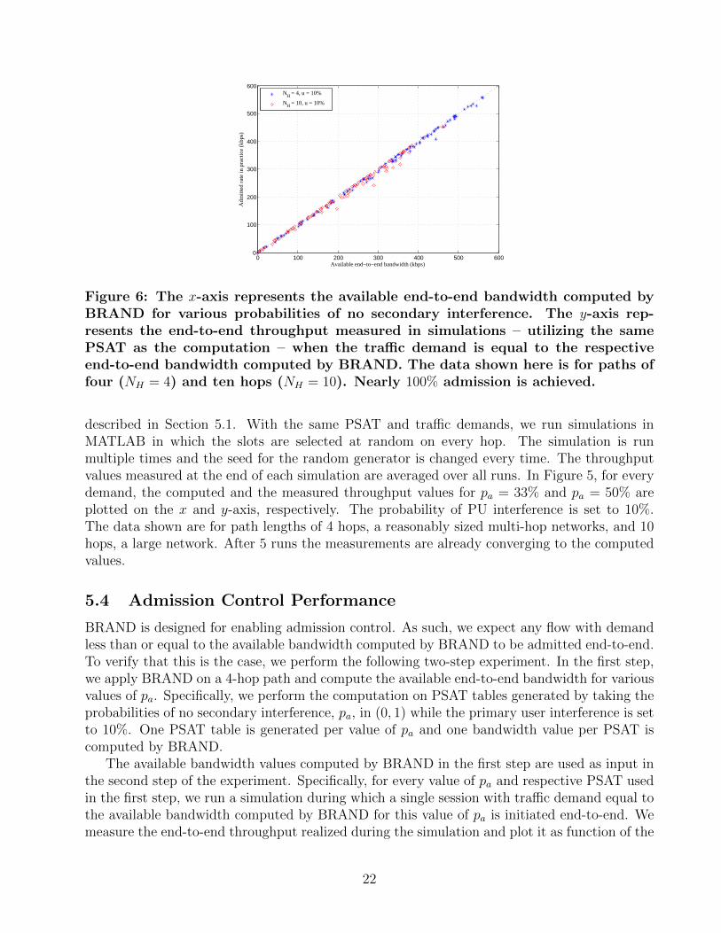
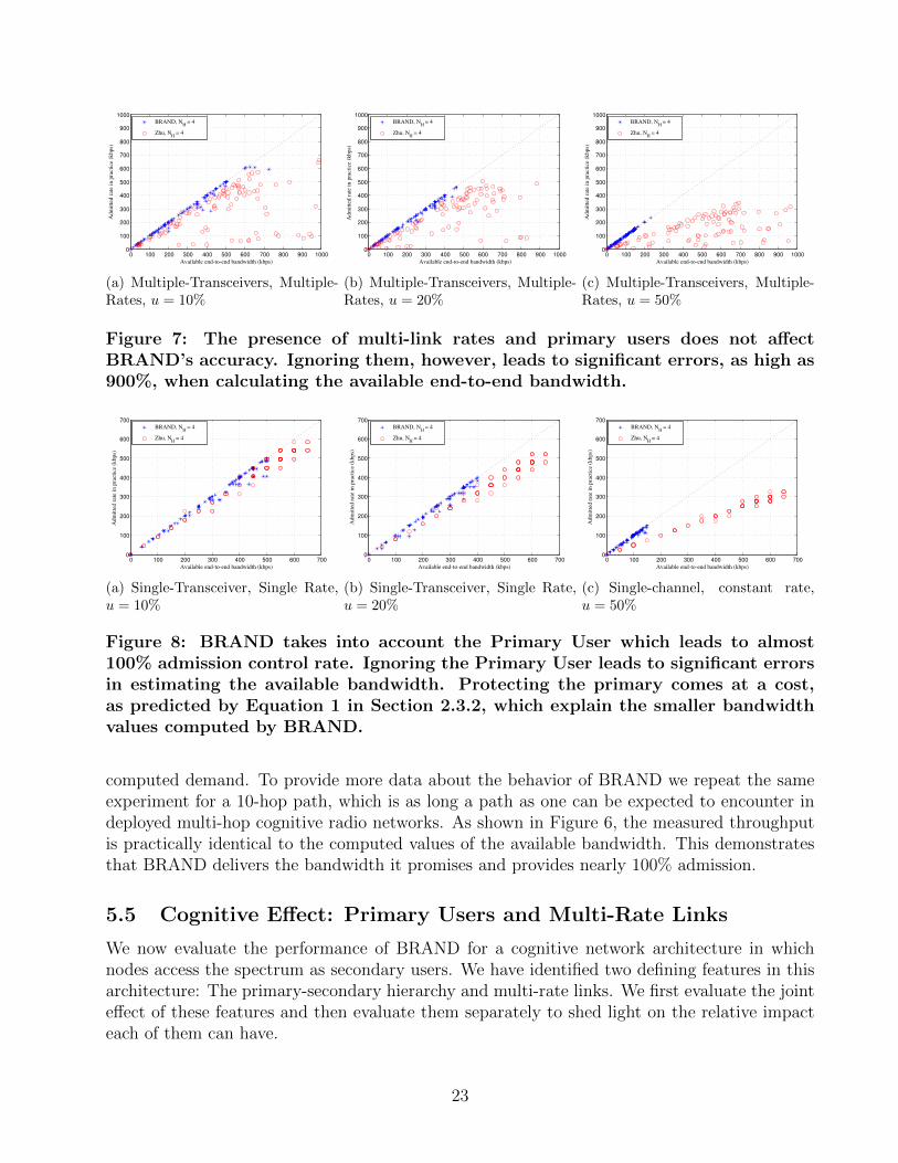
Figure 7: The presence of multi-link rates and primary users does not affectBRAND’s accuracy. Ignoring them, however, leads to significant errors, as high as900%, when calculating the available end-to-end bandwidth.
0 100 200 300 400 500 600 7000
100
200
300
400
500
600
700
Available end-to-end bandwidth (kbps)
Adm
itted
rate
in p
ract
ice
(kbp
s)
BRAND, N = 4H
Zhu, NH = 4
(a) Single-Transceiver, Single Rate,u = 10%
0 100 200 300 400 500 600 7000
100
200
300
400
500
600
700
Available end-to-end bandwidth (kbps)
Adm
itted
rate
in p
ract
ice
(kbp
s)
BRAND, N = 4H
Zhu, NH = 4
(b) Single-Transceiver, Single Rate,u = 20%
0 100 200 300 400 500 600 7000
100
200
300
400
500
600
700
Available end-to-end bandwidth (kbps)
Adm
itted
rate
in p
ract
ice
(kbp
s)
BRAND, N = 4H
Zhu, NH = 4
(c) Single-channel, constant rate,u = 50%
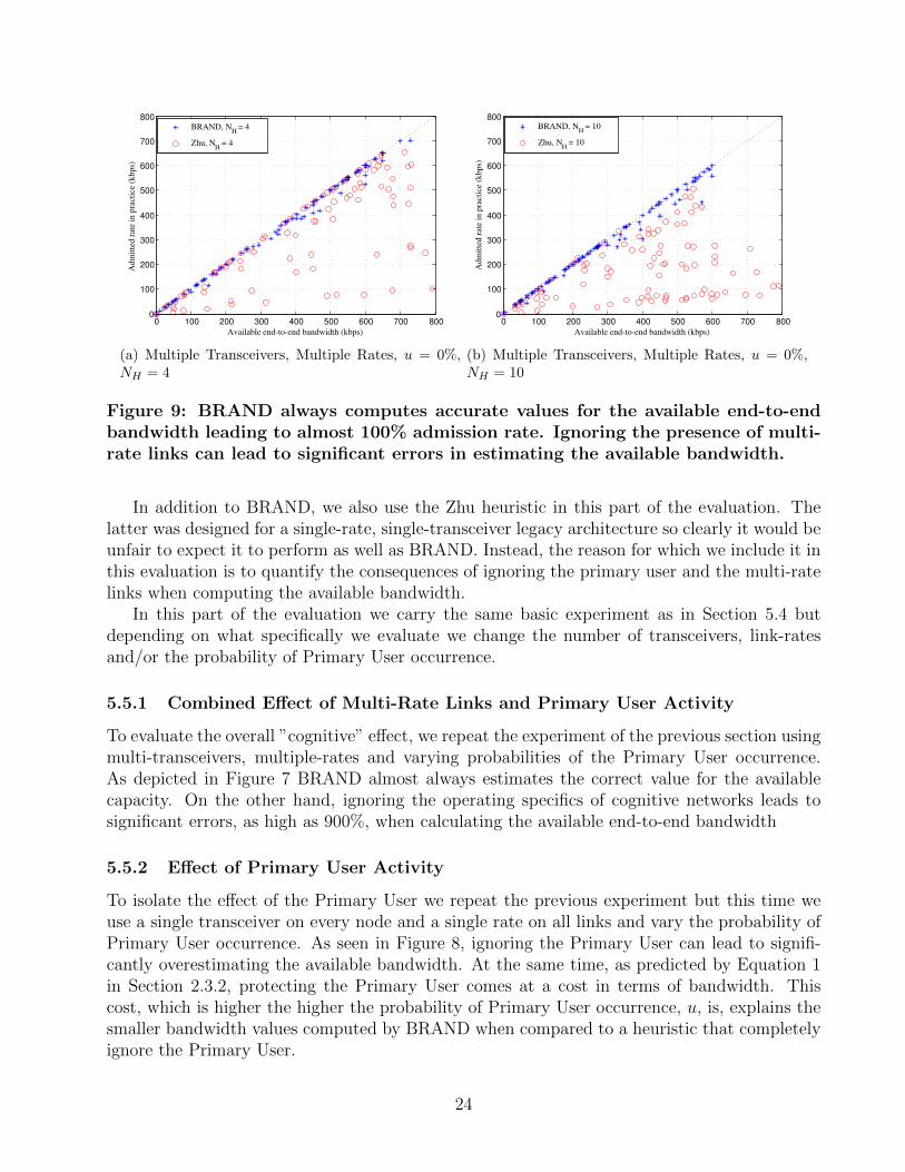
Figure 8: BRAND takes into account the Primary User which leads to almost100% admission control rate. Ignoring the Primary User leads to significant errorsin estimating the available bandwidth. Protecting the primary comes at a cost,as predicted by Equation 1 in Section 2.3.2, which explain the smaller bandwidthvalues computed by BRAND.
computed demand. To provide more data about the behavior of BRAND we repeat the sameexperiment for a 10-hop path, which is as long a path as one can be expected to encounter indeployed multi-hop cognitive radio networks. As shown in Figure 6, the measured throughputis practically identical to the computed values of the available bandwidth. This demonstratesthat BRAND delivers the bandwidth it promises and provides nearly 100% admission.
5.5 Cognitive Effect: Primary Users and Multi-Rate Links
We now evaluate the performance of BRAND for a cognitive network architecture in whichnodes access the spectrum as secondary users. We have identified two defining features in thisarchitecture: The primary-secondary hierarchy and multi-rate links. We first evaluate the jointeffect of these features and then evaluate them separately to shed light on the relative impacteach of them can have.
23
0 100 200 300 400 500 600 700 8000
100
200
300
400
500
600
700
800
Available end-to-end bandwidth (kbps)
Adm
itted
rate
in p
ract
ice
(kbp
s)BRAND, N = 4H
Zhu, NH = 4
(a) Multiple Transceivers, Multiple Rates, u = 0%,NH = 4
0 100 200 300 400 500 600 700 8000
100
200
300
400
500
600
700
800
Available end-to-end bandwidth (kbps)
Adm
itted
rate
in p
ract
ice
(kbp
s)
BRAND, N = 10H
Zhu, NH = 10
(b) Multiple Transceivers, Multiple Rates, u = 0%,NH = 10
Figure 9: BRAND always computes accurate values for the available end-to-endbandwidth leading to almost 100% admission rate. Ignoring the presence of multi-rate links can lead to significant errors in estimating the available bandwidth.
In addition to BRAND, we also use the Zhu heuristic in this part of the evaluation. Thelatter was designed for a single-rate, single-transceiver legacy architecture so clearly it would beunfair to expect it to perform as well as BRAND. Instead, the reason for which we include it inthis evaluation is to quantify the consequences of ignoring the primary user and the multi-ratelinks when computing the available bandwidth.
In this part of the evaluation we carry the same basic experiment as in Section 5.4 butdepending on what specifically we evaluate we change the number of transceivers, link-ratesand/or the probability of Primary User occurrence.
5.5.1 Combined Effect of Multi-Rate Links and Primary User Activity
To evaluate the overall ”cognitive” effect, we repeat the experiment of the previous section usingmulti-transceivers, multiple-rates and varying probabilities of the Primary User occurrence.As depicted in Figure 7 BRAND almost always estimates the correct value for the availablecapacity. On the other hand, ignoring the operating specifics of cognitive networks leads tosignificant errors, as high as 900%, when calculating the available end-to-end bandwidth
5.5.2 Effect of Primary User Activity
To isolate the effect of the Primary User we repeat the previous experiment but this time weuse a single transceiver on every node and a single rate on all links and vary the probability ofPrimary User occurrence. As seen in Figure 8, ignoring the Primary User can lead to signifi-cantly overestimating the available bandwidth. At the same time, as predicted by Equation 1in Section 2.3.2, protecting the Primary User comes at a cost in terms of bandwidth. Thiscost, which is higher the higher the probability of Primary User occurrence, u, is, explains thesmaller bandwidth values computed by BRAND when compared to a heuristic that completelyignore the Primary User.
24
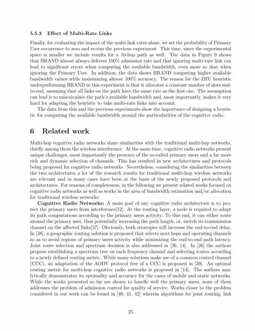
5.5.3 Effect of Multi-Rate Links
Finally, for evaluating the impact of the multi-link rates alone, we set the probability of PrimaryUser occurrence to zero and re-run the previous experiment. This time, since the experimentalspace is smaller we include results for a 10-hop path as well. The data in Figure 9 showsthat BRAND almost always delivers 100% admission rate and that ignoring multi-rate link canlead to significant errors when computing the available bandwidth, even more so that whenignoring the Primary User. In addition, the data shows BRAND computing higher availablebandwidth values while maintaining almost 100% accuracy. The reason for the ZHU heuristicunderperforming BRAND in this experiment is that it allocates a constant number of slots end-to-end, assuming that all links on the path have the same rate as the first one. The assumptioncan lead it to miscalculate the path’s available bandwidth and, most importantly, makes it veryhard for adapting the heuristic to take multi-rate links into account.
The data from this and the previous experiments show the importance of designing a heuris-tic for computing the available bandwidth around the particularities of the cognitive radio.
6 Related work
Multi-hop cognitive radio networks share similarities with the traditional multi-hop networks,chiefly among them the wireless interference. At the same time, cognitive radio networks presentunique challenges, most importantly the presence of the so-called primary users and a far morerich and dynamic selection of channels. This has resulted in new architectures and protocolsbeing proposed for cognitive radio networks. Nevertheless, considering the similarities betweenthe two architectures a lot of the research results for traditional multi-hop wireless networksare relevant and in many cases have been at the basis of the newly proposed protocols andarchitectures. For reasons of completeness, in the following we present related works focused oncognitive radio networks as well as works in the area of bandwidth estimation and/or allocationfor traditional wireless networks.
Cognitive Radio Networks: A main goal of any cognitive radio architecture is to pro-tect the primary users from interference[12]. At the routing layer, a node is required to adaptits path computations according to the primary users activity. To this end, it can either routearound the primary user, thus potentially increasing the path length, or, switch its transmissionchannel on the affected links[37]. Obviously, both strategies will increase the end-to-end delay.In [38], a geographic routing solution is proposed that selects next hops and operating channelsso as to avoid regions of primary users activity while minimizing the end-to-end path latency.Joint route selection and spectrum decision is also addressed in [26, 14]. In [26] the authorspropose establishing a spectrum tree on each frequency channel and selecting routes accordingto a newly defined routing metric. While many solutions make use of a common control channel(CCC), an adaptation of the AODV protocol free of a CCC is proposed in [39]. An optimalrouting metric for multi-hop cognitive radio networks is proposed in [14]. The authors ana-lytically demonstrates its optimality and accuracy for the cases of mobile and static networks.While the works presented so far are shown to handle well the primary users, none of themaddresses the problem of admission control for quality of service. Works closer to the problemconsidered in our work can be found in [40, 41, 42] wherein algorithms for joint routing, link
25
scheduling and spectrum assignment algorithms have been studied. In [40] an opportunisticscheduling that maximizes the overall capacity of secondary users while satisfying a constrainton time average collision rate at the primary users is proposed. In [41] the joint routing andlink scheduling problem with uncertain spectrum supply is investigated. The authors in [42]address the problem of minimizing the total transmission latency. Finally, [43] has proposed adistributed algorithm for jointly optimizing routing, scheduling, spectrum allocation and trans-mit power. Nevertheless, the problem of computing the end-to-end bandwidth of a multih-hoppath is not addressed in any of these works.
Non-Cognitive (Legacy) Networks: The problem of QoS in non-cognitive wirelessmulti-hop architectures, with a single or multiple radios, have been subject of significant re-search efforts and an exhaustive survey is beyond the scope of this paper. Instead, here wesimply summarize a subset of the published works that is closest to the work presented in thispaper. The problem of admission control for QoS routing in multi-hop networks is studiedby numerous works, including [23] and the references therein. In [23], it is shown that for aTDMA architecture, the problem of computing the residual end-to-end bandwidth for a multi-hop path is NP-Complete. Intuitively speaking, the problem is hard because computing theresidual end-to-end bandwidth is coupled with the problem of per-link slot assignments. Withthe problem being NP-Complete, a greedy heuristic is proposed and incorporated in the AODVrouting protocol. However, this heuristic was designed for a single radio, non-cognitive radioarchitecture and, as we show in Section 5, cannot be readily applied to a cognitive radio archi-tecture. In [44], the authors study the joint routing and channel assignment problem for thecase of wireless mesh networks with multiple radios. They propose a constant approximationalgorithm to the NP-hard problem of maximizing the overall network throughput, subjectedto fairness constraints. Similarly, [45] provides a distributed, online and provably efficient al-gorithm for joint routing, channel assignment and scheduling in multi-hop multi-radio ad hocnetworks. However, unlike these works, we do not propose a new routing scheme and insteadfocus on solving the problem of admission control once the paths are computed. The advantageof this approach is that it allows for a solution that can be adopted by already establishedrouting protocols.
In [46] the authors consider the problem of joint routing and link scheduling and proposea solution which consists of forming a set of constraints and solving a linear programmingproblem. A set of necessary conditions for a rate vector to be achieved is available in [47].In [24] the capacity region of multi-radio multi-channel wireless networks has been studied byintroducing a multi-dimensional conflict graph characterizing the interferences between adjacent(radio, link, channel)-tuples. An admission control scheme is provided by deriving a set of localsufficient conditions for flow feasibility in such networks. Indeed, a simple condition based onthe neighborhood constraint is first proposed, before a more accurate one is derived by adaptingthe scaled clique constraint introduced in [48]. The proposed solution can identify the feasibleflows. However, among the feasible flows it can only provide a positive answer for admission forthe ones that satisfy the sufficient conditions; there is no answer for the feasible flows that donot satisfy the sufficient conditions. What is more, in this work as well as in [46, 47], the focushas been on the offline version of the admission control problem. That is, given a network withno prior allocations, the problem considered is that of computing the maximum rate that canbe admitted between a source and a destination. In our work, we focus on the online versionof the admission control problem: Given a live network, where capacity is allocated as traffic
26
sessions arrive, the problem we tackle is that of computing the bandwidth available between asource and a destination at the time a new traffic session arrives.
7 Concluding Remarks
In this paper, we have revisited the problem of admission control for the radio cognitive context.Our solution, BRAND, uses a linear time algorithm for estimating the available end-to-endthroughput in TDMA-based multi-hop cognitive radio networks wherein each node is equippedwith multiple transceivers. We have addressed the particular case of random slots selection atthe MAC layer and provided an admission control scheme for end-to-end flows. Our method isbased on the introduced l-link available slot set decomposition and the clique sliding approach,an approximation scheme that reduces the calculation complexity from exponential to linearwhile still returning accurate and reliable results. We have shown that BRAND can run ina distributed fashion. This, coupled with our choice of computing the available bandwidthof a path, makes BRAND a feasible proposition for any routing approach. Using a thoroughnumerical analysis we have demonstrated the correctness of BRAND as well as its capability inaccurately taking into account the cognitive radio context, in particular the Primary User andmulti-rate links, and thus delivering almost 100% admission rate in a variety of conditions.
As future work we intend to explore the problem of admission control in multi-hop cognitiveradio networks from a different perspective. That is, instead of being provided the path tothe destination and computing its available bandwidth, we want to explore the problem ofcomputing the path that currently has the maximum available bandwidth among all paths tothe destination. As we remarked in Section 3, it is not clear that doing so would lead to betteroverall performance but nevertheless it is a path worth exploring.
27

28
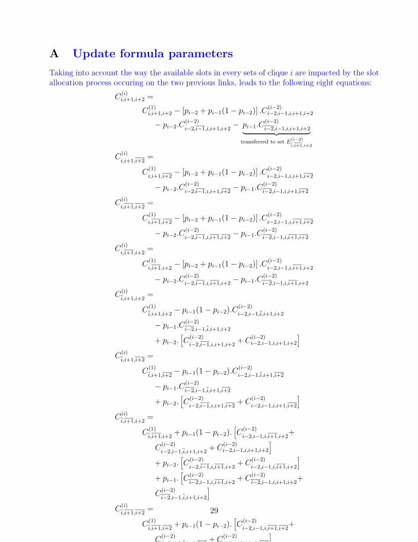
A Update formula parameters
Taking into account the way the available slots in every sets of clique i are impacted by the slotallocation process occuring on the two previous links, leads to the following eight equations:
C(i)i,i+1,i+2 =
C(1)i,i+1,i+2 − [pi−2 + pi−1(1− pi−2)] .C(i−2)
i−2,i−1,i,i+1,i+2
− pi−2.C(i−2)i−2,i−1,i,i+1,i+2
− pi−1.C(i−2)i−2,i−1,i,i+1,i+2︸ ︷︷ ︸
transferred to set E(i−2)
i,i+1,i+2
C(i)
i,i+1,i+2=
C(1)
i,i+1,i+2− [pi−2 + pi−1(1− pi−2)] .C(i−2)
i−2,i−1,i,i+1,i+2
− pi−2.C(i−2)i−2,i−1,i,i+1,i+2
− pi−1.C(i−2)i−2,i−1,i,i+1,i+2
C(i)
i,i+1,i+2=
C(1)
i,i+1,i+2− [pi−2 + pi−1(1− pi−2)] .C(i−2)
i−2,i−1,i,i+1,i+2
− pi−2.C(i−2)i−2,i−1,i,i+1,i+2
− pi−1.C(i−2)i−2,i−1,i,i+1,i+2
C(i)
i,i+1,i+2=
C(1)
i,i+1,i+2− [pi−2 + pi−1(1− pi−2)] .C(i−2)
i−2,i−1,i,i+1,i+2
− pi−2.C(i−2)i−2,i−1,i,i+1,i+2
− pi−1.C(i−2)i−2,i−1,i,i+1,i+2
C(i)
i,i+1,i+2=
C(1)
i,i+1,i+2− pi−1(1− pi−2).C(i−2)
i−2,i−1,i,i+1,i+2
− pi−1.C(i−2)i−2,i−1,i,i+1,i+2
+ pi−2.[C
(i−2)i−2,i−1,i,i+1,i+2
+ C(i−2)i−2,i−1,i,i+1,i+2
]C
(i)
i,i+1,i+2=
C(1)
i,i+1,i+2− pi−1(1− pi−2).C(i−2)
i−2,i−1,i,i+1,i+2
− pi−1.C(i−2)i−2,i−1,i,i+1,i+2
+ pi−2.[C
(i−2)i−2,i−1,i,i+1,i+2
+ C(i−2)i−2,i−1,i,i+1,i+2
]C
(i)
i,i+1,i+2=
C(1)
i,i+1,i+2+ pi−1(1− pi−2).
[C
(i−2)i−2,i−1,i,i+1,i+2
+
C(i−2)i−2,i−1,i,i+1,i+2
+ C(i−2)i−2,i−1,i,i+1,i+2
]+ pi−2.
[C
(i−2)i−2,i−1,i,i+1,i+2
+ C(i−2)i−2,i−1,i,i+1,i+2
]+ pi−1.
[C
(i−2)i−2,i−1,i,i+1,i+2
+ C(i−2)i−2,i−1,i,i+1,i+2
+
C(i−2)i−2,i−1,i,i+1,i+2
]C
(i)
i,i+1,i+2=
C(1)
i,i+1,i+2+ pi−1(1− pi−2).
[C
(i−2)i−2,i−1,i,i+1,i+2
+
C(i−2)i−2,i−1,i,i+1,i+2
+ C(i−2)i−2,i−1,i,i+1,i+2
]+ pi−2.
[C
(i−2)i−2,i−1,i,i+1,i+2
+ C(i−2)i−2,i−1,i,i+1,i+2
]+ pi−1.
[C
(i−2)i−2,i−1,i,i+1,i+2
+ C(i−2)i−2,i−1,i,i+1,i+2
+
C(i−2)i−2,i−1,i,i+1,i+2
]
29
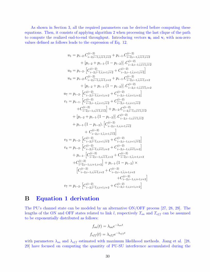
As shown in Section 3, all the required parameters can be derived before computing theseequations. Then, it consists of applying algorithm 2 when processing the last clique of the pathto compute the realized end-to-end throughput. Introducing vectors ui and vi with non-zerovalues defined as follows leads to the expression of Eq. 12.
u1 = pi−2.C(i−2)i−2,i−1,i,i+1,i+2
+ pi−1.C(i−2)i−2,i−1,i,i+1,i+2
+ [pi−2 + pi−1.(1− pi−2)] .C(i−2)i−2,i−1,i,i+1,i+2
u3 = pi−2.[C
(i−2)i−2,i−1,i,i+1,i+2
+ C(i−2)i−2,i−1,i,i+1,i+2
]u4 = pi−2.C
(i−2)i−2,i−1,i,i+1,i+2
+ pi−1.C(i−2)i−2,i−1,i,i+1,i+2
+ [pi−2 + pi−1.(1− pi−2)] .C(i−2)i−2,i−1,i,i+1,i+2
u7 = pi−2.[C
(i−2)i−2,i−1,i,i+1,i+2
+ C(i−2)i−2,i−1,i,i+1,i+2
]v1 = pi−1.
[C
(i−2)i−2,i−1,i,i+1,i+2
+ C(i−2)i−2,i−1,i,i+1,i+2
+C(i−2)i−2,i−1,i,i+1,i+2
]+ pi−2.C
(i−2)i−2,i−1,i,i+1,i+2
+ [pi−2 + pi−1.(1− pi−2)] .C(i−2)i−2,i−1,i,i+1,i+2
+ pi−1.(1− pi−2).[C
(i−2)i−2,i−1,i,i+1,i+2
+ C(i−2)i−2,i−1,i,i+1,i+2
]v3 = pi−2.
[C
(i−2)i−2,i−1,i,i+1,i+2
+ C(i−2)i−2,i−1,i,i+1,i+2
]v4 = pi−2.
[C
(i−2)i−2,i−1,i,i+1,i+2
+ C(i−2)i−2,i−1,i,i+1,i+2
]+ pi−1.
[C
(i−2)i−2,i−1,i,i+1,i+2
+ C(i−2)i−2,i−1,i,i+1,i+2
+C(i−2)i−2,i−1,i,i+1,i+2
]+ pi−1.(1− pi−2)×[
C(i−2)i−2,i−1,i,i+1,i+2
+ C(i−2)i−2,i−1,i,i+1,i+2
+C(i−2)i−2,i−1,i,i+1,i+2
]v7 = pi−2.
[C
(i−2)i−2,i−1,i,i+1,i+2
+ C(i−2)i−2,i−1,i,i+1,i+2
]
B Equation 1 derivation
The PU’s channel state can be modeled by an alternative ON/OFF process [27, 28, 29]. Thelengths of the ON and OFF states related to link l, respectively Ton and Toff can be assumedto be exponentially distributed as follows:
fon(t) = λone−λont
foff (t) = λoffe−λoff t
with parameters λon and λoff estimated with maximum likelihood methods. Jiang et al. [28,29] have focused on computing the quantity of PU-SU interference accumulated during the
30
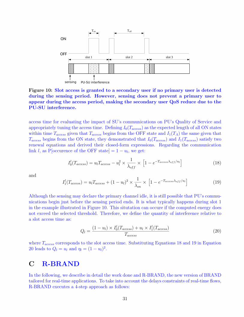
ON
OFFslot 1 slot 2 slot 3
Ton Toff
sensing PU-SU interference
Figure 10: Slot access is granted to a secondary user if no primary user is detectedduring the sensing period. However, sensing does not prevent a primary user toappear during the access period, making the secondary user QoS reduce due to thePU-SU interference.
access time for evaluating the impact of SU’s communications on PU’s Quality of Service andappropriately tuning the access time. Defining I0(Taccess) as the expected length of all ON stateswithin time Taccess given that Taccess begins from the OFF state and I1(TA) the same given thatTaccess begins from the ON state, they demonstrated that I0(Taccess) and I1(Taccess) satisfy tworenewal equations and derived their closed-form expressions. Regarding the communicationlink l, as P[occurence of the OFF state] = 1− ul, we get:
I l0(Taccess) = ulTaccess − u2l ×1
λoff×[1− e−Taccessλoff/ul
](18)
and
I l1(Taccess) = ulTaccess + (1− ul)2 ×1
λon×[1− e−Taccessλoff/ul
](19)
Although the sensing may declare the primary channel idle, it is still possible that PU’s commu-nications begin just before the sensing period ends. It is what typically happens during slot 1in the example illustrated in Figure 10. This situtation can occure if the computed energy doesnot exceed the selected threshold. Therefore, we define the quantity of interference relative toa slot access time as:
Ql =(1− ul)× I l0(Taccess) + ul × I l1(Taccess)
Taccess(20)
where Taccess corresponds to the slot access time. Substituting Equations 18 and 19 in Equation20 leads to Ql = ul and ηl = (1− ul)2.
C R-BRAND
In the following, we describe in detail the work done and R-BRAND, the new version of BRANDtailored for real-time applications. To take into account the delays constraints of real-time flows,R-BRAND executes a 4-step approach as follows:
31
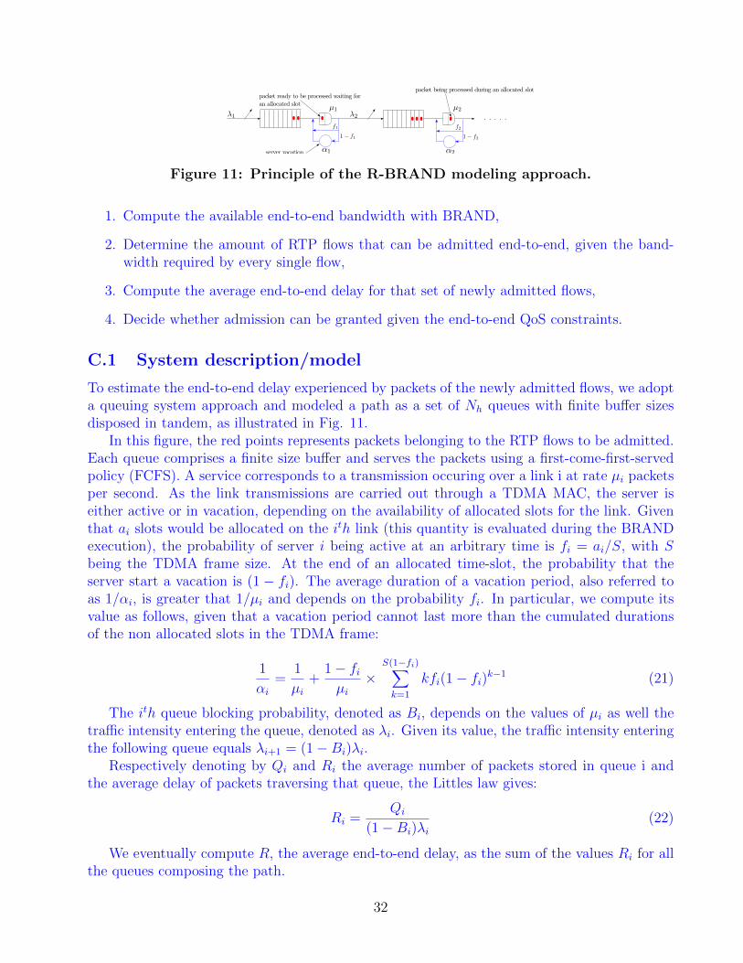
packet ready to be processed waiting foran allocated slot
server vacation
packet being processed during an allocated slot
Figure 11: Principle of the R-BRAND modeling approach.
1. Compute the available end-to-end bandwidth with BRAND,
2. Determine the amount of RTP flows that can be admitted end-to-end, given the band-width required by every single flow,
3. Compute the average end-to-end delay for that set of newly admitted flows,
4. Decide whether admission can be granted given the end-to-end QoS constraints.
C.1 System description/model
To estimate the end-to-end delay experienced by packets of the newly admitted flows, we adopta queuing system approach and modeled a path as a set of Nh queues with finite buffer sizesdisposed in tandem, as illustrated in Fig. 11.
In this figure, the red points represents packets belonging to the RTP flows to be admitted.Each queue comprises a finite size buffer and serves the packets using a first-come-first-servedpolicy (FCFS). A service corresponds to a transmission occuring over a link i at rate µi packetsper second. As the link transmissions are carried out through a TDMA MAC, the server iseither active or in vacation, depending on the availability of allocated slots for the link. Giventhat ai slots would be allocated on the ith link (this quantity is evaluated during the BRANDexecution), the probability of server i being active at an arbitrary time is fi = ai/S, with Sbeing the TDMA frame size. At the end of an allocated time-slot, the probability that theserver start a vacation is (1 − fi). The average duration of a vacation period, also referred toas 1/αi, is greater that 1/µi and depends on the probability fi. In particular, we compute itsvalue as follows, given that a vacation period cannot last more than the cumulated durationsof the non allocated slots in the TDMA frame:
1
αi=
1
µi+
1− fiµi×
S(1−fi)∑k=1
kfi(1− fi)k−1 (21)
The ith queue blocking probability, denoted as Bi, depends on the values of µi as well thetraffic intensity entering the queue, denoted as λi. Given its value, the traffic intensity enteringthe following queue equals λi+1 = (1−Bi)λi.
Respectively denoting by Qi and Ri the average number of packets stored in queue i andthe average delay of packets traversing that queue, the Littles law gives:
Ri =Qi
(1−Bi)λi(22)
We eventually compute R, the average end-to-end delay, as the sum of the values Ri for allthe queues composing the path.
32
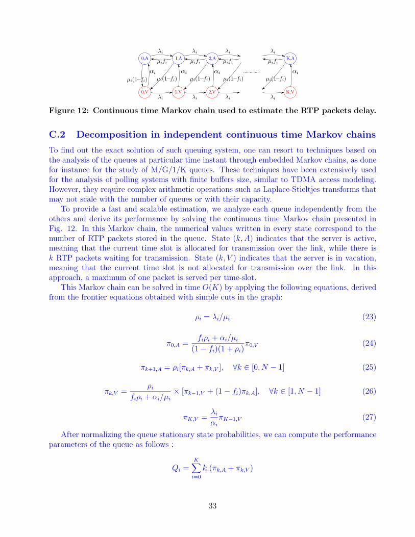
1,A
1,V
2,A
2,V
K,A
K,V0,V
0,A
Figure 12: Continuous time Markov chain used to estimate the RTP packets delay.
C.2 Decomposition in independent continuous time Markov chains
To find out the exact solution of such queuing system, one can resort to techniques based onthe analysis of the queues at particular time instant through embedded Markov chains, as donefor instance for the study of M/G/1/K queues. These techniques have been extensively usedfor the analysis of polling systems with finite buffers size, similar to TDMA access modeling.However, they require complex arithmetic operations such as Laplace-Stieltjes transforms thatmay not scale with the number of queues or with their capacity.
To provide a fast and scalable estimation, we analyze each queue independently from theothers and derive its performance by solving the continuous time Markov chain presented inFig. 12. In this Markov chain, the numerical values written in every state correspond to thenumber of RTP packets stored in the queue. State (k,A) indicates that the server is active,meaning that the current time slot is allocated for transmission over the link, while there isk RTP packets waiting for transmission. State (k, V ) indicates that the server is in vacation,meaning that the current time slot is not allocated for transmission over the link. In thisapproach, a maximum of one packet is served per time-slot.
This Markov chain can be solved in time O(K) by applying the following equations, derivedfrom the frontier equations obtained with simple cuts in the graph:
ρi = λi/µi (23)
π0,A =fiρi + αi/µi
(1− fi)(1 + ρi)π0,V (24)
πk+1,A = ρi[πk,A + πk,V ], ∀k ∈ [0, N − 1] (25)
πk,V =ρi
fiρi + αi/µi× [πk−1,V + (1− fi)πk,A], ∀k ∈ [1, N − 1] (26)
πK,V =λiαiπK−1,V (27)
After normalizing the queue stationary state probabilities, we can compute the performanceparameters of the queue as follows :
Qi =K∑i=0
k.(πk,A + πk,V )
33
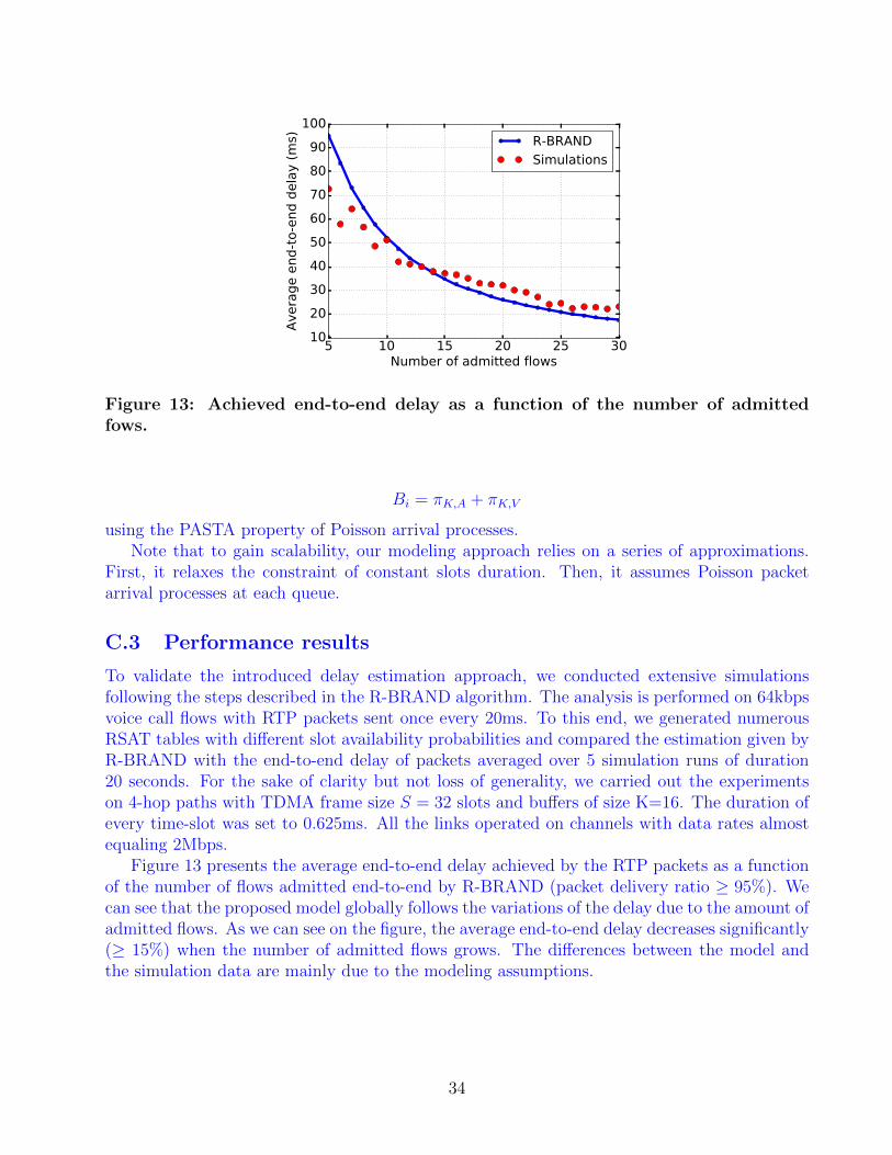
5 10 15 20 25 30Number of admitted flows
10
20
30
40
50
60
70
80
90
100
Avera
ge e
nd-t
o-e
nd d
ela
y (
ms) R-BRAND
Simulations
Figure 13: Achieved end-to-end delay as a function of the number of admittedfows.
Bi = πK,A + πK,V
using the PASTA property of Poisson arrival processes.Note that to gain scalability, our modeling approach relies on a series of approximations.
First, it relaxes the constraint of constant slots duration. Then, it assumes Poisson packetarrival processes at each queue.
C.3 Performance results
To validate the introduced delay estimation approach, we conducted extensive simulationsfollowing the steps described in the R-BRAND algorithm. The analysis is performed on 64kbpsvoice call flows with RTP packets sent once every 20ms. To this end, we generated numerousRSAT tables with different slot availability probabilities and compared the estimation given byR-BRAND with the end-to-end delay of packets averaged over 5 simulation runs of duration20 seconds. For the sake of clarity but not loss of generality, we carried out the experimentson 4-hop paths with TDMA frame size S = 32 slots and buffers of size K=16. The duration ofevery time-slot was set to 0.625ms. All the links operated on channels with data rates almostequaling 2Mbps.
Figure 13 presents the average end-to-end delay achieved by the RTP packets as a functionof the number of flows admitted end-to-end by R-BRAND (packet delivery ratio ≥ 95%). Wecan see that the proposed model globally follows the variations of the delay due to the amount ofadmitted flows. As we can see on the figure, the average end-to-end delay decreases significantly(≥ 15%) when the number of admitted flows grows. The differences between the model andthe simulation data are mainly due to the modeling assumptions.
34

D Integer program formulation for the case of 4-hop
paths
Setting up the following variables
x = (x1, x2, . . . , x23)T
b =
C
(1)
1,2,3,4+ C
(1)
1,2,3,4
C(1)
1,2,3,4
C(1)
1,2,3,4
C(1)
1,2,3,4+ C
(1)
1,2,3,4
A =
1 0 1 0 0 0 0 0 0 0 1 0 0 1 0 1 0 0 0 0 1 0 00 1 0 0 1 0 1 0 0 0 0 1 0 0 1 0 0 1 0 0 0 1 00 0 0 1 0 1 0 0 1 0 0 0 1 0 0 0 1 0 1 0 0 0 10 0 0 0 0 0 0 1 0 1 0 0 0 1 0 1 0 0 0 1 1 0 0
and
P =
φ1f1/S 0 0 0
0 φ2f2/S 0 00 0 φ3f3/S 00 0 0 φ4f4/S
we have used lpsolve 5.5 to realize the following objective and evaluate the maximum availablebandwidth provided by an optimal slot allocation process
maximizex
min (P. {A.x + b})
subject to x1 + x2 ≤ C(1)
1,2,3,4,
x3 + x4 ≤ C(1)
1,2,3,4,
x5 + x6 ≤ C(1)
1,2,3,4,
x7 + x8 ≤ C(1)
1,2,3,4,
x9 + x10 ≤ C(1)
1,2,3,4,
x11 + x12 + x13 ≤ C(1)
1,2,3,4,
x14 + x15 ≤ C(1)
1,2,3,4,
x16 + x17 ≤ C(1)
1,2,3,4,
x18 + x19 + x20 ≤ C(1)
1,2,3,4,
x21 + x22 + x23 ≤ C(1)1,2,3,4,
xi integer and positive.
35
References
[1] B. Wang and K. Liu, “Advances in cognitive radio networks: A survey,” IEEE Journal ofSelected Topics in Signal Processing, vol. 5, no. 1, pp. 5–23, feb. 2011.
[2] “Evaluation of the Performance of Prototype TV-Band White Space Devices,” FCCpress release, November 2008. [Online]. Available: http://hraunfoss.fcc.gov/edocs public/attachmatch/FCC-08-260A6.pdf
[3] “Digital agenda: Commission moves to foster wireless innovation through sharing of radiospectrumh,” European Commission Press release, September 2012. [Online]. Available:http://europa.eu/rapid/press-release IP-12-929 en.htm?locale=en
[4] P. Bahl, R. Chandra, T. Moscibroda, R. Murty, and M. Welsh, “White space networkingwith wi-fi like connectivity,” in ACM SIGCOMM 2009. New York, NY, USA: ACM,2009, pp. 27–38.
[5] “Report to the president: Realizing the full potential of government-held spectrum tospur economic growth,” President’s Council of Advisors on Science and Technology,July 2012. [Online]. Available: http://www.whitehouse.gov/sites/default/files/microsites/ostp/pcast spectrum report final july 20 2012.pdf
[6] I. Mitola, J. and J. Maguire, G.Q., “Cognitive radio: making software radios more per-sonal,” IEEE Personal Communications, vol. 6, no. 4, pp. 13–18, aug 1999.
[7] I. F. Akyildiz, W.-Y. Lee, M. C. Vuran, and S. Mohanty, “Next generation/dynamic spec-trum access/cognitive radio wireless networks: A survey,” Computer Networks, vol. 50,no. 13, pp. 2127–2159, 2006.
[8] J. Marinho and E. Monteiro, “Cognitive radio: survey on communication protocols, spec-trum decision issues, and future research directions,” Wirel. Netw., vol. 18, no. 2, pp.147–164, Feb. 2012.
[9] A. De Domenico, E. Strinati, and M. Di Benedetto, “A survey on MAC strategies forcognitive radio networks,” Communications Surveys Tutorials, IEEE, vol. 14, no. 1, pp.21–44, 2012.
[10] Y. Zhao, M. Song, and C. Xin, “FMAC: A fair MAC protocol for coexisting cognitive radionetworks,” in INFOCOM, 2013 Proceedings IEEE, 2013, pp. 1474–1482.
[11] X. Zhang and H. Su, “CREAM-MAC: Cognitive radio-enabled multi-channel MAC proto-col over dynamic spectrum access networks,” Selected Topics in Signal Processing, IEEEJournal of, vol. 5, no. 1, pp. 110–123, 2011.
[12] K. Chowdhury and I. Akyildiz, “CRP: A Routing Protocol for Cognitive Radio Ad HocNetworks,” IEEE Journal on Selected Areas in Communications, vol. 29, no. 4, pp. 794–804, april 2011.
36
[13] Y. Liu, L. Cai, and X. Shen, “Joint channel selection and opportunistic forwarding in multi-hop cognitive radio networks,” in Global Telecommunications Conference (GLOBECOM2011), 2011 IEEE, 2011, pp. 1–5.
[14] M. Caleffi, I. F. Akyildiz, and L. Paura, “OPERA: Optimal Routing Metric for CognitiveRadio Ad Hoc Networks,” IEEE Transactions on Wireless Communications, vol. 11, no. 8,pp. 2884–2894, 2012.
[15] S. Soltani and M. W. Mutka, “Primary weight measure and its support in stochasticrouting for dynamic cognitive radio networks,” in Proceedings of the 1st ACM workshopon Cognitive radio architectures for broadband, ser. CRAB ’13. New York, NY, USA:ACM, 2013, pp. 69–78.
[16] M. Youssef, M. Ibrahim, M. Abdelatif, L. Chen, and A. Vasilakos, “Routing metrics ofcognitive radio networks: A survey,” Communications Surveys Tutorials, IEEE, vol. PP,no. 99, pp. 1–18, 2013.
[17] “IEEE Standard for Information Technology–Telecommunications and information ex-change between systems Wireless Regional Area Networks (WRAN)–specific requirementspart 22: Cognitive wireless RAN medium access control (MAC) and physical layer (PHY)specifications: Policies and procedures for operation in the TV bands,” IEEE Std 802.22-2011, pp. 1–680, January 2011.
[18] J. Redi and R. Ramanathan, “The DARPA WNaN network architecture,” in IEEE MIL-COM 2011, nov. 2011, pp. 2258–2263.
[19] C. Cordeiro and K. Challapali, “C-MAC: A Cognitive MAC Protocol for Multi-ChannelWireless Networks,” in DySPAN 2007, april 2007, pp. 147–157.
[20] Y. Kondareddy and P. Agrawal, “Synchronized MAC Protocol For Multi-Hop CognitiveRadio Networks,” in IEEE ICC ’08, may 2008, pp. 3198–3202.
[21] T. Chen, H. Zhang, G. Maggio, and I. Chlamtac, “Cogmesh: A cluster-based cognitiveradio network,” in New Frontiers in Dynamic Spectrum Access Networks, 2007. DySPAN2007. 2nd IEEE International Symposium on, 2007, pp. 168–178.
[22] B. Hamdaoui and K. Shin, “OS-MAC: An efficient MAC protocol for spectrum-agile wire-less networks,” Mobile Computing, IEEE Transactions on, vol. 7, no. 8, pp. 915–930, 2008.
[23] C. Zhu and M. Corson, “QoS routing for mobile ad hoc networks,” in INFOCOM 2002,vol. 2, 2002, pp. 958–967.
[24] H. Li, Y. Cheng, P.-J. Wan, and J. Cao, “Local sufficient rate constraints for guaran-teed capacity region in multi-radio multi-channel wireless networks,” in INFOCOM, 2011Proceedings IEEE, 2011, pp. 990–998.
[25] I. Rhee, A. Warrier, J. Min, and L. Xu, “DRAND: distributed randomized TDMA schedul-ing for wireless ad-hoc networks,” in ACM MobiHoc ’06. New York, NY, USA: ACM,2006, pp. 190–201.
37
[26] G.-M. Zhu, I. F. Akyildiz, and G.-S. Kuo, “STOD-RP: A Spectrum-Tree Based On-Demand Routing Protocol for Multi-Hop Cognitive Radio Networks,” in GLOBECOM,2008, pp. 3086–3090.
[27] H. Kim and K. G. Shin, “Efficient discovery of spectrum opportunities with mac-layersensing in cognitive radio networks,” IEEE Transactions on Mobile Computing, vol. 7,no. 5, pp. 533–545, May 2008.
[28] C. Jiang, Y. Chen, Y. Gao, and K. J. R. Liu, “Joint spectrum sensing and access evolution-ary game in cognitive radio networks,” IEEE Transactions on Wireless Communications,vol. 12, no. 5, pp. 2470–2483, 2013.
[29] C. Jiang, Y. Chen, K. J. R. Liu, and Y. Ren, “Renewal-theoretical dynamic spectrumaccess in cognitive radio network with unknown primary behavior,” IEEE Journal onSelected Areas in Communications, vol. 31, no. 3, pp. 406–416, 2013.
[30] R. Murty, R. Chandra, T. Moscibroda, and P. Bahl, “Senseless: A database-driven whitespaces network,” Mobile Computing, IEEE Transactions on, vol. 11, no. 2, pp. 189–203,2012.
[31] J. Jia, Q. Zhang, and X. Shen, “Hc-mac: A hardware-constrained cognitive mac for efficientspectrum management,” Selected Areas in Communications, IEEE Journal on, vol. 26,no. 1, pp. 106–117, 2008.
[32] H. Bany Salameh, M. Krunz, and O. Younis, “Mac protocol for opportunistic cognitiveradio networks with soft guarantees,” Mobile Computing, IEEE Transactions on, vol. 8,no. 10, pp. 1339–1352, 2009.
[33] D. Maltz, J. Broch, J. Jetcheva, and D. Johnson, “The effects of on-demand behavior inrouting protocols for multihop wireless ad hoc networks,” Selected Areas in Communica-tions, IEEE Journal on, vol. 17, no. 8, pp. 1439–1453, 1999.
[34] P. Jacquet, P. Muhlethaler, T. Clausen, A. Laouiti, A. Qayyum, and L. Viennot, “Opti-mized link state routing protocol for ad hoc networks,” in Multi Topic Conference, 2001.IEEE INMIC 2001. Technology for the 21st Century. Proceedings. IEEE International,2001, pp. 62–68.
[35] C. Perkins and E. Royer, “Ad-hoc on-demand distance vector routing,” in Mobile Comput-ing Systems and Applications, 1999. Proceedings. WMCSA ’99. Second IEEE Workshopon, 1999, pp. 90–100.
[36] M. Berkelaar, K. Eikland, and P. Notebaert, “lp solve 5.5, open source (mixed-integer) linear programming system,” Software, May 1 2004. [Online]. Available:http://lpsolve.sourceforge.net/5.5/
[37] H. Khalife, N. Malouch, and S. Fdida, “Multihop cognitive radio networks: to route or notto route,” Netwrk. Mag. of Global Internetwkg., vol. 23, no. 4, pp. 20–25, Jul. 2009.
38
[38] K. R. Chowdhury and M. D. Felice, “Search: A routing protocol for mobile cognitive radioad-hoc networks,” Computer Communications, vol. 32, no. 18, pp. 1983–1997, 2009.
[39] A. S. Cacciapuoti, C. Calcagno, M. Caleffi, and L. Paura, “CAODV: Routing in mobile ad-hoc cognitive radio networks,” in IFIP Wireless Days 2010, Venice, Italy, October 20-22,2010. IEEE, 2010, pp. 1–5.
[40] D. Xue and E. Ekici, “Guaranteed opportunistic scheduling in multi-hop cognitive radionetworks,” in INFOCOM, 2011, pp. 2984–2992.
[41] M. Pan, C. Zhang, P. Li, and Y. Fang, “Joint routing and link scheduling for cognitiveradio networks under uncertain spectrum supply,” in INFOCOM, 2011, pp. 2237–2245.
[42] W. Li, X. Cheng, T. Jing, Y. Cui, K. Xing, and W. Wang, “Spectrum Assignment andSharing for Delay Minimization in Multi-Hop Multi-Flow CRNs,” IEEE Journal on Se-lected Areas in Communications (JSAC), Special Issue on Cognitive Radio, March 2013.
[43] L. Ding, T. Melodia, S. Batalama, and M. J. Medley, “ROSA: distributed joint routingand dynamic spectrum allocation in cognitive radio ad hoc networks,” in ACM MSWiM2009. New York, NY, USA: ACM, 2009, pp. 13–20.
[44] M. Alicherry, R. Bhatia, and L. E. Li, “Joint channel assignment and routing for through-put optimization in multi-radio wireless mesh networks,” in MobiCom ’05. New York,NY, USA: ACM, 2005, pp. 58–72.
[45] X. Lin and S. B. Rasool, “Distributed and provably efficient algorithms for jointchannel-assignment, scheduling, and routing in multichannel ad hoc wireless networks,”IEEE/ACM Trans. Netw., vol. 17, no. 6, pp. 1874–1887, Dec. 2009.
[46] M. Kodialam and T. Nandagopal, “Characterizing achievable rates in multi-hop wirelessnetworks: the joint routing and scheduling problem,” in MobiCom ’03. New York, NY,USA: ACM, 2003, pp. 42–54.
[47] ——, “Characterizing the capacity region in multi-radio multi-channel wireless mesh net-works,” in MobiCom ’05. New York, NY, USA: ACM, 2005, pp. 73–87.
[48] R. Gupta, J. Musacchio, and J. Walrand, “Sufficient rate constraints for qos flows in ad-hocnetworks,” Ad Hoc Netw., vol. 5, no. 4, pp. 429–443, May 2007.
39