ggplotStatistical Computing

Package used

• Install the package: “install.packages(ggplot2)”• Use the package: “library(ggplot2)”

ggplot Part I

Scatter plot

Scatterplot

• Use the following syntax

p <- ggplot(data, aes(x = variable name 1, y = variable name 2))p <- p+geom_point(aes())p

• Assign variables to aesthetics colour, size, and shape

MPG Example

• Use the following syntax

library(ggplot2)

## Warning: package 'ggplot2' was built under R version 3.5.2

data(mpg)head(mpg)

## # A tibble: 6 x 11## manufacturer model displ year cyl trans drv cty hwy fl class## <chr> <chr> <dbl> <int> <int> <chr> <chr> <int> <int> <chr> <chr>## 1 audi a4 1.8 1999 4 auto(~ f 18 29 p comp~## 2 audi a4 1.8 1999 4 manua~ f 21 29 p comp~## 3 audi a4 2 2008 4 manua~ f 20 31 p comp~## 4 audi a4 2 2008 4 auto(~ f 21 30 p comp~## 5 audi a4 2.8 1999 6 auto(~ f 16 26 p comp~## 6 audi a4 2.8 1999 6 manua~ f 18 26 p comp~

1

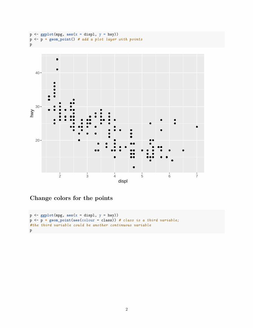
p <- ggplot(mpg, aes(x = displ, y = hwy))p <- p + geom_point() # add a plot layer with pointsp

20

30

40

2 3 4 5 6 7displ

hwy

Change colors for the points

p <- ggplot(mpg, aes(x = displ, y = hwy))p <- p + geom_point(aes(colour = class)) # class is a third variable;#the third variable could be another continuous variablep

2

20

30

40

2 3 4 5 6 7displ

hwy

class

2seater

compact

midsize

minivan

pickup

subcompact

suv

Change sizes for the points

• Assign variables to aesthetics colour, size, and shape

p <- ggplot(mpg, aes(x = displ, y = hwy))p <- p + geom_point(aes(size = cyl)) # cyl is a third variable which must be discretep

3

20

30

40

2 3 4 5 6 7displ

hwy

cyl

4

5

6

7

8

Change shapes for the points

• Assign variables to aesthetics colour, size, and shape

p <- ggplot(mpg, aes(x = displ, y = hwy))p <- p + geom_point(aes(shape = drv)) # drv is a third variable which must be discretep

4

20

30

40

2 3 4 5 6 7displ

hwy

drv

4

f

r

Add lines and smoothing band to the plot

• Assign variables to aesthetics colour, size, and shape

p <- ggplot(mpg, aes(x = displ, y = hwy))p <- p + geom_point(aes(shape = drv))p <- p + geom_line() + stat_smooth(colour = "blue", span = 0.2)p

## `geom_smooth()` using method = 'loess' and formula 'y ~ x'

5

20

30

40

2 3 4 5 6 7displ

hwy

drv

4

f

r

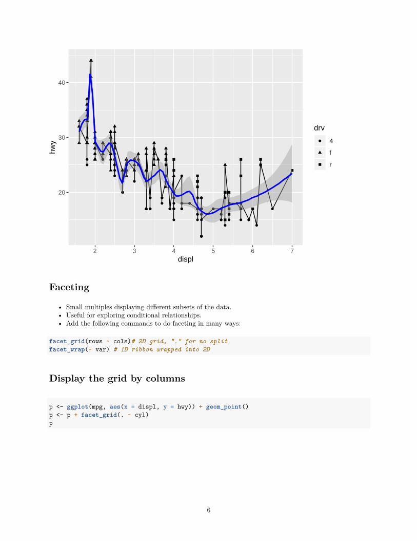
Faceting

• Small multiples displaying different subsets of the data.• Useful for exploring conditional relationships.• Add the following commands to do faceting in many ways:

facet_grid(rows ~ cols)# 2D grid, "." for no splitfacet_wrap(~ var) # 1D ribbon wrapped into 2D

Display the grid by columns

p <- ggplot(mpg, aes(x = displ, y = hwy)) + geom_point()p <- p + facet_grid(. ~ cyl)p

6

4 5 6 8

2 3 4 5 6 7 2 3 4 5 6 7 2 3 4 5 6 7 2 3 4 5 6 7

20

30

40

displ

hwy

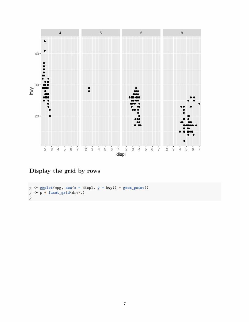
Display the grid by rows

p <- ggplot(mpg, aes(x = displ, y = hwy)) + geom_point()p <- p + facet_grid(drv~.)p

7

4f

r

2 3 4 5 6 7

20

30

40

20

30

40

20

30

40

displ

hwy

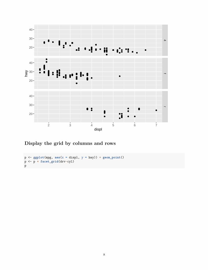
Display the grid by columns and rows

p <- ggplot(mpg, aes(x = displ, y = hwy)) + geom_point()p <- p + facet_grid(drv~cyl)p

8

4 5 6 8

4f

r

2 3 4 5 6 7 2 3 4 5 6 7 2 3 4 5 6 7 2 3 4 5 6 7

20

30

40

20

30

40

20

30

40

displ

hwy

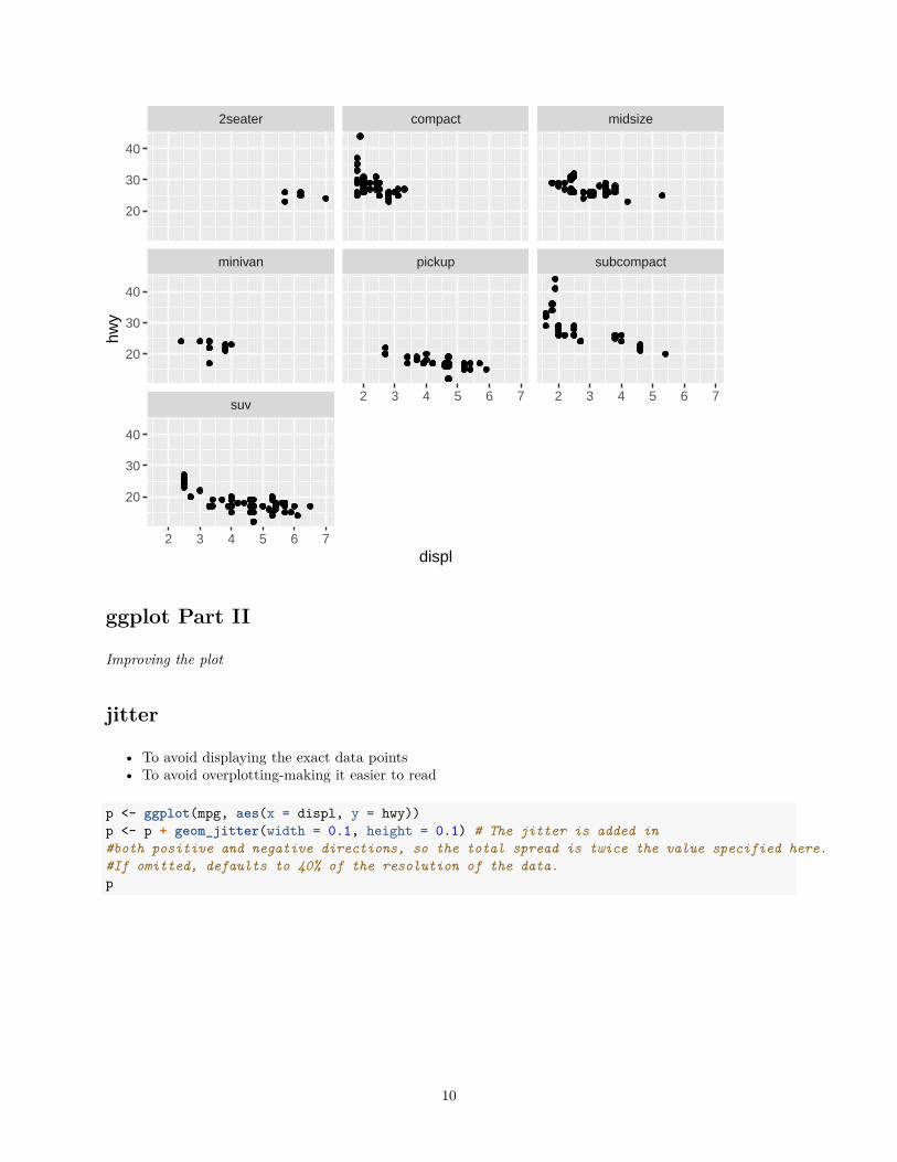
Display the grid by natural layouts

p <- ggplot(mpg, aes(x = displ, y = hwy)) + geom_point()p <- p + facet_wrap(~class)p

9

suv

minivan pickup subcompact

2seater compact midsize

2 3 4 5 6 7

2 3 4 5 6 7 2 3 4 5 6 7

20

30

40

20

30

40

20

30

40

displ

hwy

ggplot Part II

Improving the plot

jitter

• To avoid displaying the exact data points• To avoid overplotting-making it easier to read

p <- ggplot(mpg, aes(x = displ, y = hwy))p <- p + geom_jitter(width = 0.1, height = 0.1) # The jitter is added in#both positive and negative directions, so the total spread is twice the value specified here.#If omitted, defaults to 40% of the resolution of the data.p

10

20

30

40

2 3 4 5 6 7displ

hwy

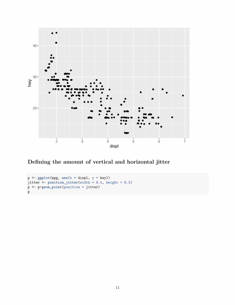
Defining the amount of vertical and horizontal jitter

p <- ggplot(mpg, aes(x = displ, y = hwy))jitter <- position_jitter(width = 0.1, height = 0.1)p <- p+geom_point(position = jitter)p

11

20

30

40

2 3 4 5 6 7displ

hwy

Make the jitter repreducible

p <- ggplot(mpg, aes(x = displ, y = hwy))jitter <- position_jitter(width = 0.1, height = 0.1, seed = 123)p <- p+geom_point(position = jitter)p

12

20

30

40

2 3 4 5 6 7displ

hwy

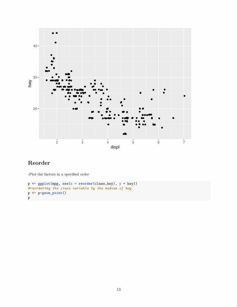
Reorder

-Plot the factors in a specified order

p <- ggplot(mpg, aes(x = reorder(class,hwy), y = hwy))#reordering the class variable by the median of hwyp <- p+geom_point()p

13

20

30

40

pickup suv minivan 2seater midsize subcompact compactreorder(class, hwy)

hwy

Reorder

-Plot the factors in a specified order

p <- ggplot(mpg, aes(x = reorder(class,hwy, FUN = median), y = hwy))#reordering the class variable by the median of hwyp <- p+geom_point()p

14

20

30

40

pickup suv minivan 2seater subcompact compact midsizereorder(class, hwy, FUN = median)

hwy

ggplot

Boxplot

Reorder

-Preparing data

data("ToothGrowth")ToothGrowth$dose <- as.factor(ToothGrowth$dose)head(ToothGrowth)

## len supp dose## 1 4.2 VC 0.5## 2 11.5 VC 0.5## 3 7.3 VC 0.5## 4 5.8 VC 0.5## 5 6.4 VC 0.5## 6 10.0 VC 0.5

15

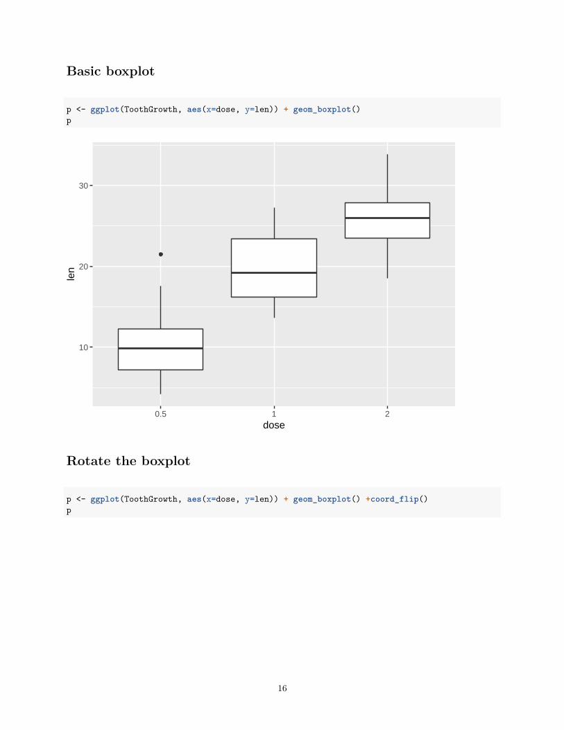
Basic boxplot

p <- ggplot(ToothGrowth, aes(x=dose, y=len)) + geom_boxplot()p

10

20

30

0.5 1 2dose

len

Rotate the boxplot

p <- ggplot(ToothGrowth, aes(x=dose, y=len)) + geom_boxplot() +coord_flip()p

16

0.5

1

2

10 20 30len

dose

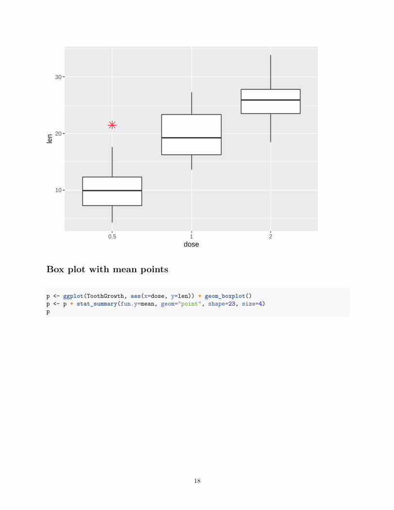
Change outlier, color, shape and size

p <- ggplot(ToothGrowth, aes(x=dose, y=len)) +geom_boxplot(outlier.colour="red", outlier.shape=8,

outlier.size=4)p

17

10

20

30

0.5 1 2dose

len

Box plot with mean points

p <- ggplot(ToothGrowth, aes(x=dose, y=len)) + geom_boxplot()p <- p + stat_summary(fun.y=mean, geom="point", shape=23, size=4)p

18

10

20

30

0.5 1 2dose

len

Box plot with standard deviation points

p <- ggplot(ToothGrowth, aes(x=dose, y=len)) + geom_boxplot()p <- p + stat_summary(fun.y=sd, geom="point", shape=23, size=4)p

19

10

20

30

0.5 1 2dose

len

Adding other statistics summaries to the plot

• https://www.rdocumentation.org/packages/Hmisc/versions/4.2-0/topics/smean.sd• https://www.rdocumentation.org/packages/ggplot2/versions/0.9.1/topics/stat_summary

Choose which items to display

p <- ggplot(ToothGrowth, aes(x=dose, y=len)) + geom_boxplot()p + scale_x_discrete(limits=c("0.5", "2"))

## Warning: Removed 20 rows containing missing values (stat_boxplot).

20

10

20

30

0.5 2dose

len

Boxplot with dots

p <- ggplot(ToothGrowth, aes(x=dose, y=len)) + geom_boxplot()p + geom_dotplot(binaxis='y', stackdir='center', dotsize=1)

## `stat_bindot()` using `bins = 30`. Pick better value with `binwidth`.

21

10

20

30

0.5 1 2dose

len

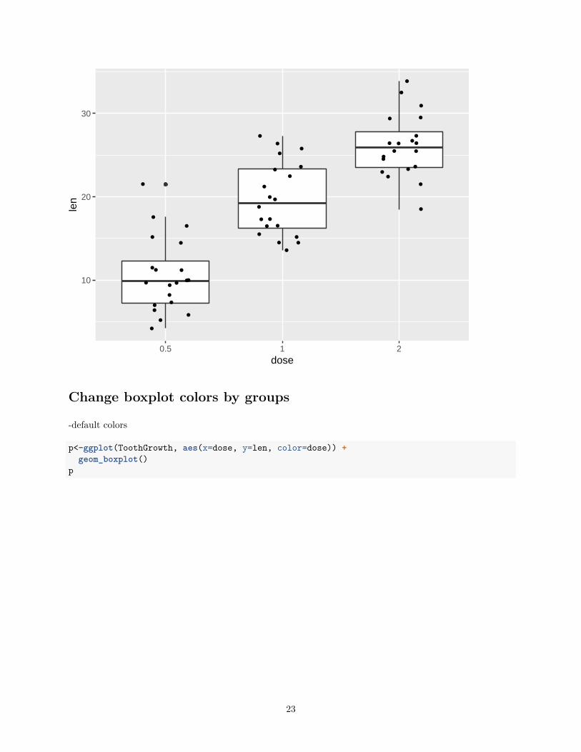
Boxplot with jittered dots

p <- ggplot(ToothGrowth, aes(x=dose, y=len)) + geom_boxplot()p + geom_jitter(shape=16, position=position_jitter(0.2))

22

10

20

30

0.5 1 2dose

len

Change boxplot colors by groups

-default colors

p<-ggplot(ToothGrowth, aes(x=dose, y=len, color=dose)) +geom_boxplot()

p

23

10

20

30

0.5 1 2dose

len

dose

0.5

1

2

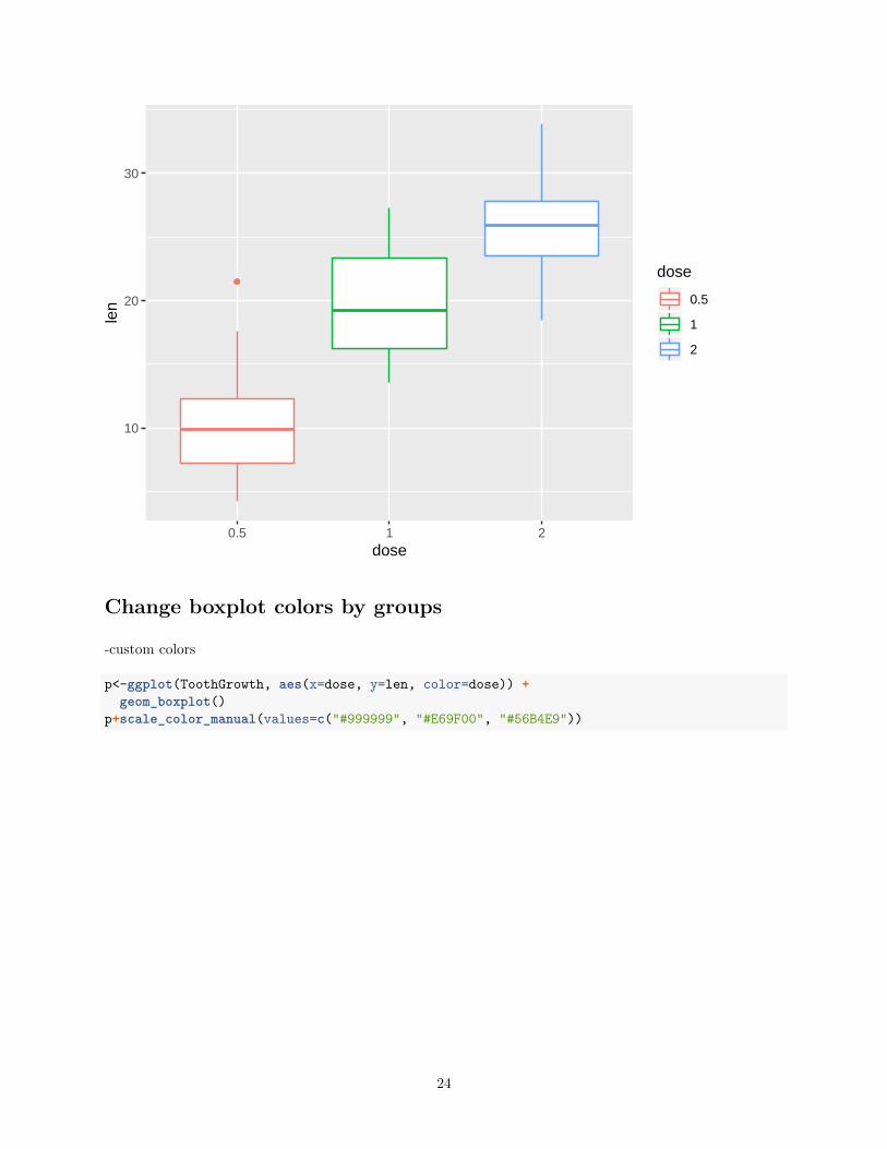
Change boxplot colors by groups

-custom colors

p<-ggplot(ToothGrowth, aes(x=dose, y=len, color=dose)) +geom_boxplot()

p+scale_color_manual(values=c("#999999", "#E69F00", "#56B4E9"))

24

10

20

30

0.5 1 2dose

len

dose

0.5

1

2

Change boxplot colors by groups

-grey colors

p<-ggplot(ToothGrowth, aes(x=dose, y=len, color=dose)) +geom_boxplot()p + scale_color_grey() + theme_classic()

25

10

20

30

0.5 1 2dose

len

dose

0.5

1

2

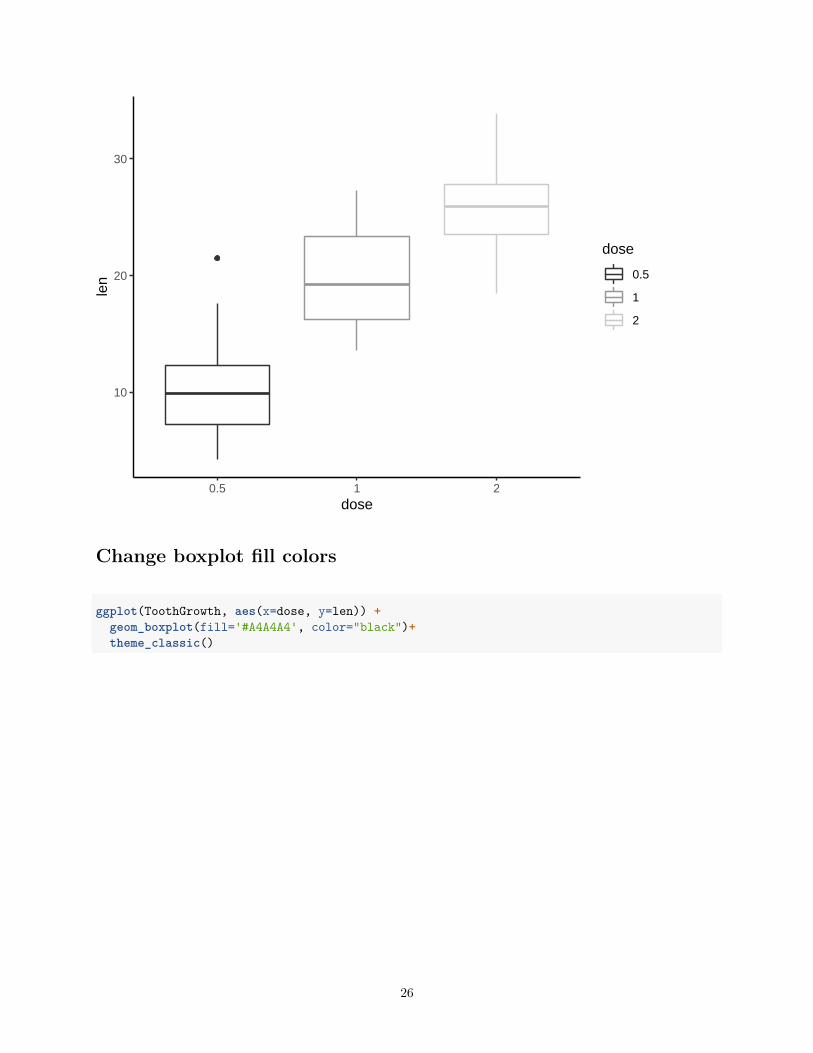
Change boxplot fill colors

ggplot(ToothGrowth, aes(x=dose, y=len)) +geom_boxplot(fill='#A4A4A4', color="black")+theme_classic()

26

10

20

30

0.5 1 2dose

len

Change boxplot fill colors by groups

-grey

p <- ggplot(ToothGrowth, aes(x=dose, y=len, fill=dose)) +geom_boxplot()

p + scale_fill_grey() + theme_classic()

27

10

20

30

0.5 1 2dose

len

dose

0.5

1

2

Change boxplot fill colors by groups

-custom colors

p<-ggplot(ToothGrowth, aes(x=dose, y=len, fill=dose)) +geom_boxplot()

p+scale_fill_manual(values=c("#999999", "#E69F00", "#56B4E9"))

28

10

20

30

0.5 1 2dose

len

dose

0.5

1

2

Change the legend position

p<-ggplot(ToothGrowth, aes(x=dose, y=len, fill=dose)) +geom_boxplot()

p + theme(legend.position="bottom") # or "bottom" or "none"

29

10

20

30

0.5 1 2dose

len

dose 0.5 1 2

Change the order of items in the legend

p<-ggplot(ToothGrowth, aes(x=dose, y=len)) +geom_boxplot()p + scale_x_discrete(limits=c("2", "0.5", "1"))

30

10

20

30

2 0.5 1dose

len

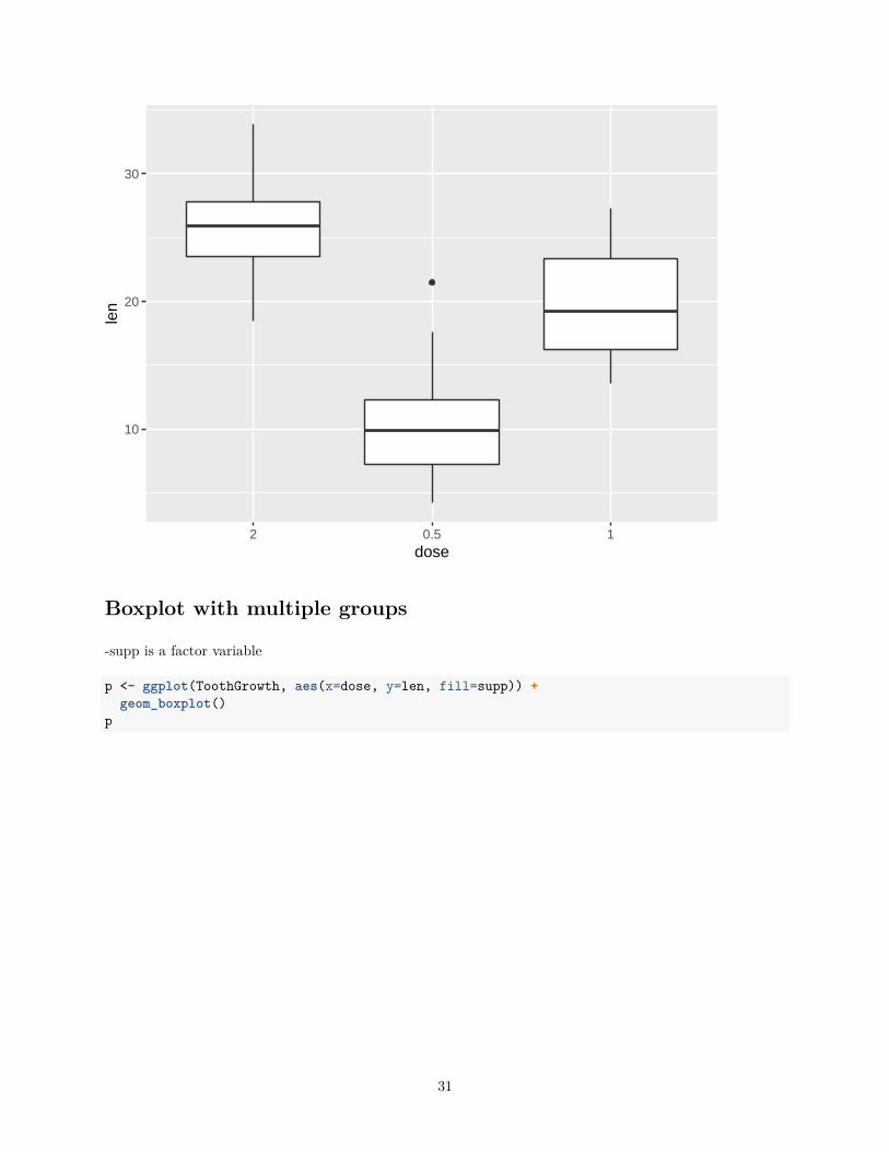
Boxplot with multiple groups

-supp is a factor variable

p <- ggplot(ToothGrowth, aes(x=dose, y=len, fill=supp)) +geom_boxplot()

p

31

10

20

30

0.5 1 2dose

len

supp

OJ

VC

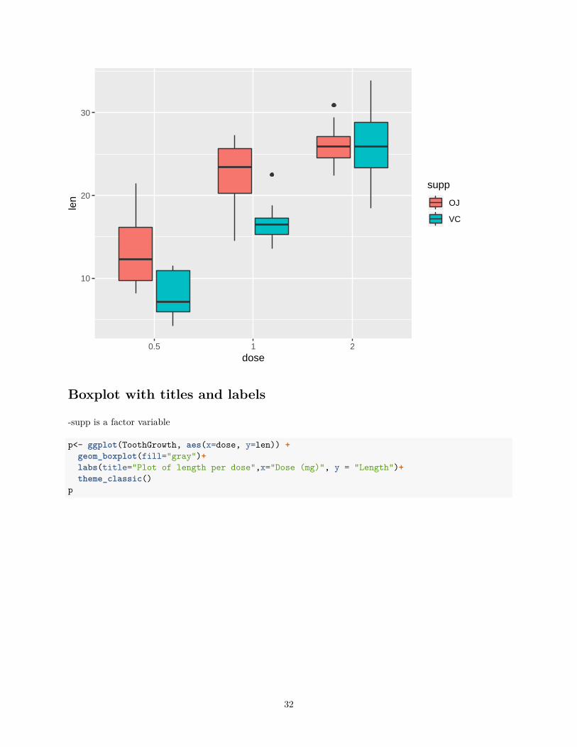
Boxplot with titles and labels

-supp is a factor variable

p<- ggplot(ToothGrowth, aes(x=dose, y=len)) +geom_boxplot(fill="gray")+labs(title="Plot of length per dose",x="Dose (mg)", y = "Length")+theme_classic()

p

32

10

20

30

0.5 1 2Dose (mg)

Leng

thPlot of length per dose

Smoothing density plot

data("diamonds")p<- ggplot(diamonds, aes(depth, colour = cut)) +

geom_density() +xlim(55, 70)p

## Warning: Removed 45 rows containing non-finite values (stat_density).

33

0.0

0.2

0.4

0.6

55 60 65 70depth

dens

ity

cut

Fair

Good

Very Good

Premium

Ideal

Smoothing density plot

data("diamonds")ggplot(diamonds, aes(depth, fill = cut, colour = cut)) +

geom_density(alpha = 0.1) +xlim(55, 70)

## Warning: Removed 45 rows containing non-finite values (stat_density).

34

0.0

0.2

0.4

0.6

55 60 65 70depth

dens

ity

cut

Fair

Good

Very Good

Premium

Ideal

35