Statistical Consulting Topics

The Bootstrap...

“The bootstrap is a computer-based methodfor assigning measures of accuracy to sta-tistical estimates.” (Efron and Tibshrani,1998.)

•What do we do when our distributionalassumptions about our model are not met?

• The assumptions are needed to give us...

– valid standard errors

– valid confidence intervals

– valid hypothesis tests and p-values

1

• Consider inference on a mean µ with the es-timator X from an i.i.d random sample.

– X is a random variable

– Define the statistic: T = X−µs/√n

– If the population from which we are draw-ing is normally distributed, we have:T ∼ tn−1 which we use to...

∗ form valid 100(1− α)% CI’s on µ

∗ perform α-level hypothesis tests on µ

– Without normality, we can not assume Thas this distribution (its dist’n is unknown)

– How can we do inference?

2

• The Bootstrap method can be used for es-timating a sampling distribution when thetheoretical sampling distribution is unknown.

Recall, a sampling distribution is...

the probability distribution of a statistic.

Examples (true under certain conditions):

1. X ∼ N(µ, σ2

n )

2. β ∼ N(β, V (β))

These sampling distributions allow us toperform hypothesis tests and form confidenceintervals on parameters of interest.

If ‘conditions’ are not met, we can still per-form statistical inference by using the bootstrap.

3

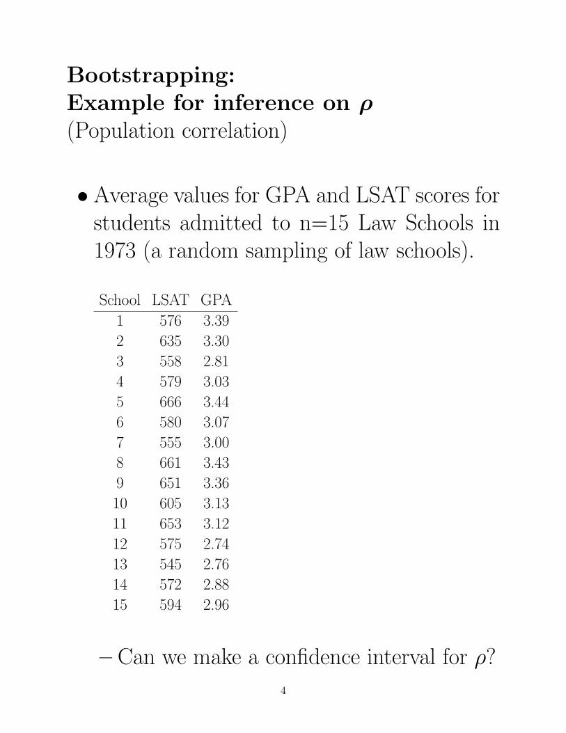
Bootstrapping:Example for inference on ρ(Population correlation)

• Average values for GPA and LSAT scores forstudents admitted to n=15 Law Schools in1973 (a random sampling of law schools).

School LSAT GPA

1 576 3.39

2 635 3.30

3 558 2.81

4 579 3.03

5 666 3.44

6 580 3.07

7 555 3.00

8 661 3.43

9 651 3.36

10 605 3.13

11 653 3.12

12 575 2.74

13 545 2.76

14 572 2.88

15 594 2.96

– Can we make a confidence interval for ρ?

4

– Point estimate for ρ is the sample correla-tion r:

r = 0.7766

●

●

●

●

●

●

●

●

●

● ●

●●

●

●

560 580 600 620 640 660

2.8

3.0

3.2

3.4

LSAT

GP

A

– Classical inference (like confidence inter-vals) on ρ depends on X and Y having abivariate normal distribution.

– In the above sample, there are a few out-liers suggesting this assumption may beviolated.

– We’ll use the bootstrap approach to dostatistical inference instead.

5

– Sampling n=15 new cases as (xi, yi) withreplacement from my original data, I cre-ate a new bootstapped data set and cal-culate r which I will label as r∗1 .

– Repeating this process 1000 times providesan empirical ‘sampling distribution’ for theestimator r (empirical means based on the ob-

served data).

r∗1 , r∗2 , r∗3 , . . . , r

∗1000

The distribution of the above values givesus an idea of the variability of our estima-tor r.

– We will assume these n = 15 observationsis a representative sample from the pop-ulation of all law schools (the assumptionwe make).

6

– The distribution of r∗1 , r∗2 , . . . , r

∗1000 is the

empirical sampling distribution of our es-timator r.

Histogram of bootstrapped.r.values

bootstrapped.r.values

Frequency

0.2 0.4 0.6 0.8 1.0

050

100

150

Observed r

– We can use it to make a 95% empiricalconfidence interval for ρ.> quantile(bootstrapped.r.values,0.025, type=3)

2.5%

0.4419053

> quantile(bootstrapped.r.values,0.975, type=3)

97.5%

0.9623332

7

– We were able to create a CI without anyassumptions on distribution, i.e. nonpara-metrically (very useful in many situations).

– This only works if the original sample isrepresentative of the original population.

– Recall what sampling variability of an es-timator is... BEFORE we collect our data,the estimator is a random variable becauseit’s value depends on the sample chosen.

– The bootstrap method uses resampling toget a handle on this variability (since wecan’t get at it theoretically because our as-sumptions weren’t met).

– We should resample from the n observa-tions in the same manner as how the origi-nal data was sampled (here, we had a sim-ple random sample).

8

Classical test of H0 : ρ = 0 (option 1)

• Built on the assumption that X and Y fol-low a bivariate normal distribution withθ = (µX , µY , σ

2X , σ

2Y , ρ).

• ρ = r, and

r =

∑i(Xi − X)(Yi − Y )√∑

i(Xi − X)2∑i(Yi − Y )2

• Test of H0 : ρ = 0

T = r√n− 2/

√1− r2

Under H0, T ∼ tn−2

This is the same t-test as H0 : β1 = 0 insimple linear regression.

9

Classical confidence interval (CI) for ρ

• r is obviously not normally distributed.

• Fisher’s z-transformation of r:

Zr = 12log(1+r

1−r)

• Zr is approx N(12log(1+ρ

1−ρ), 1n−3)

• Transformation creates approximatenormality, and variance independent of ρ

– 100(1-α)% CI for Zr is

Zr ± zα/2

√1

n−3

– To get CI for ρ, invert transformation oflower limit and upper limit for Zr using

r =(e2Zr − 1)

(e2Zr + 1)

10

Classical test of H0 : ρ = ρo (option 2)

• Based on Fisher’s Zr

• Test statistic:

Z =√n− 3(Zr − 1

2log(1+ρo1−ρo))

Under Ho, Z ∼ N(0, 1)

11

Compare CIs from Fisher’s Zr and Bootstrap

• 95% CI based on Fisher’s Zr:

If our observed data is bivariate normal, then

Zr is approx N(12log(1+ρ

1−ρ), 1n−3)

and our 95% CI for 12log(1+ρ

1−ρ) is

(0.4710, 1.6026)

and our 95% CI for ρ is

(0.4399, 0.9221).

• 95% CI based on Bootstrap (shown earlier):

(0.4419, 0.9623).

12

• If our observed data is bivariate normal, thenthe distribution of transformed bootstrappedcorrelations Z∗r,is should be approximatelynormally distributed where

Z∗r,i = 12log(

1+r∗i1−r∗i

).

Histogram of Z.r.bootstrapped

Z.r.bootstrapped

Frequency

-0.5 0.0 0.5 1.0 1.5 2.0 2.5 3.0

050

100

150

200

µZ∗r

= 1.1112 and σ2Z∗

r= 0.1435

And σ2Z∗r ,F isher

= 1n−3 = 0.0833

13

– The variance of the bootstrap distributionis slightly larger than expected by Fisher.

– TheZ∗r,i distribution is visually non-normal

(though only slightly).

This suggests that the bootstrap may be abetter option for inference than using theFisher transformation which assumed the bi-variate normal.

• Is this a way to check assumptions in complexmodels? (Classical CI vs. Bootstrap CI)

– I’ve seen it used in that way (pharmaceu-tical drug modeling, for instance).

– Not really checking the full ‘distribution’of estimators.

– Perhaps as a way to say it definitely DOESN’Tmatch assumptions.

14

• Some comments...

– The type of bootstrapping described here(case resampling) considers the regressorsX ’s to be random, not fixed.

– There are numerous types of bootstrap-ping methods that relate to how you createthe bootstrapped data sets, such as, para-metric bootstrap, semi-parametric boot-strap, wild bootstrap, or moving block boot-strap.

– The intention is for a bootstrapped dataset to represent another new hypotheticaldata set that could have just as easily beenobserved as the original data set.

– If you have known correlation in your data(non-independence), this must be accountedfor in your bootstrapping procedure.

15

– There are bias correction methods forestimates and confidence intervals.

– The Bootstrap can fail:

∗ Initial random sample not representa-tive of population

∗ Sample too small, empirical CDF too‘jagged’ (might be fixed with smooth-ing)

∗ Application of the Bootstrap did not ad-equately replicate the random processthat produced the original sample

16

Changepoint example:

In streams, the sediment (sand, gravel, rocks,etc.) that moves along the bottom (bed) of thestream is called the bedload. The bedload is dis-tinct from suspended load (in the water) andwash load (near the top of the water).

How quickly the bedload moves in a stream(bedload transport, kg/s) is dependent on theflow of the water (discharge, m3/s) and a vari-ety of other factors.

17

The bedload transport has been described asoccurring in phases, with a changepoint oc-curring at the flow where the stream transitionsfrom phase I to phase II.

“The fitted line for less-than-breakpoint flows had a

lower slope with less variance due to the fact that

bedload at these discharges consist primarily of

small quantities of sand-sized materials. In contrast,

the fitted line for flows greater than the breakpoint

had a significantly steeper slope and more variability

in transport rates due to the physical breakup of the

armor layer, the availability of subsurface material,

and subsequent changes in both the size and volume

of sediment in transport[3].”

18

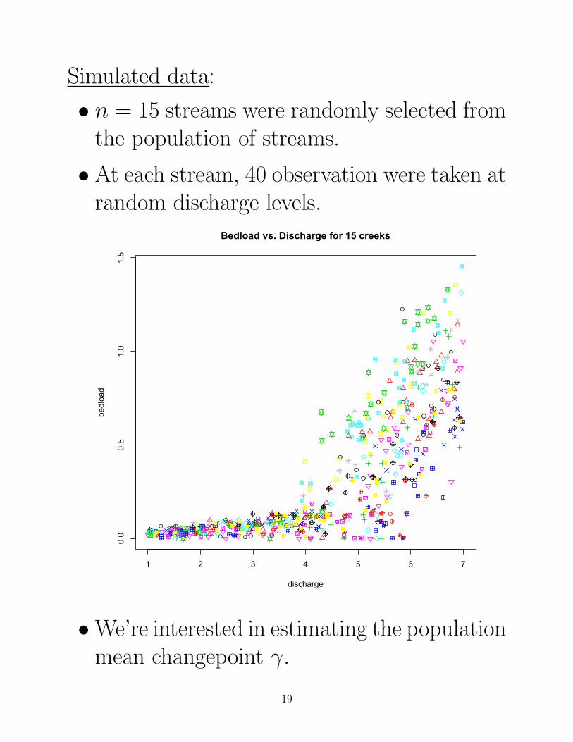
Simulated data:

• n = 15 streams were randomly selected fromthe population of streams.

• At each stream, 40 observation were taken atrandom discharge levels.

1 2 3 4 5 6 7

0.0

0.5

1.0

1.5

Bedload vs. Discharge for 15 creeks

discharge

bedload

•We’re interested in estimating the populationmean changepoint γ.

19

Applying the Bootstrap method for inference:

1. Calculate a γ from the observed data as

γobs =∑15i=1 γi15 .

2. Generate B bootstrap samples and calculateγb for each bootstrap sample b = 1, . . . , B.

Two thoughts...

(a) Bootstrapping the 15 estimated change-points (B=500).

Histogram of bootstrapped (B=500) mean changepoint

bootstrapped mean changepoint for n=15 (40 obs each creek)

Frequency

4.0 4.2 4.4 4.6 4.8 5.0

020

4060

80100

20

(b) Bootstrapping the 15 creeks and bootstrap-ping the observations within each creek.

Histogram of bootstrapped (B=500) mean changepoint

bootstrapped mean changepoint for n=15 (40 obs each creek)

Frequency

4.0 4.2 4.4 4.6 4.8 5.0

020

4060

80100

95% Bootstrap Confidence intervals:

(a) (4.214, 4.811)

(b) (4.162, 4.744)

95% Confidence interval based on normality:

(4.183, 4.844)

21

• References:

[1] Efron, B. and R.J. Tibshirani (1998). An intro-duction to Bootstrap. Chapman & Hall.

[2] Muggeo, V. (2008). Segmented: an R packageto fit regression models with broken-line relation-ships. R News, 8, 1:20-25.

[3] Ryan, S.E. and L.S. Porth (2007). A tutorial onthe piecewise regression approach applied to bed-load transport data. USDA, General TechnicalReport RMRS-GTR-189.

22