statistical inference using stochastic gradient descent ... · statistical inference using...
TRANSCRIPT

Technical Report 144
Statistical Inference Using Stochastic Gradient Descent: Volumes 1 and 2
Research Supervisor Constantine Caramanis Wireless Networking & Communications Group
Project Title: Statistical Inference Using Stochastic Gradient Descent
September 2018

Data-Supported Transportation Operations & Planning Center (D-STOP)
A Tier 1 USDOT University Transportation Center at The University of Texas at Austin
D-STOP is a collaborative initiative by researchers at the Center for Transportation Research and the Wireless Networking and Communications Group at The University of Texas at Austin.

Technical Report Documentation Page
1. Report No. D-STOP/2018/144
2. Government Accession No.
3. Recipient's Catalog No.
4. Title and Subtitle Statistical Inference Using Stochastic Gradient Descent: Volumes 1 and 2
5. Report Date October 2018 6. Performing Organization Code
7. Author(s) Natalia Ruiz Juri, Stephen D. Boyles, Tengkuo Zhu, Kenneth Perrine, Amber Chen, Yun Li
8. Performing Organization Report No. Report 144
9. Performing Organization Name and Address Data-Supported Transportation Operations & Planning Center (D-STOP) The University of Texas at Austin 3925 W. Braker Lane, 4th Floor Austin, Texas 78759
10. Work Unit No. (TRAIS) 11. Contract or Grant No. DTRT13-G-UTC58
12. Sponsoring Agency Name and Address United States Department of Transportation University Transportation Centers 1200 New Jersey Avenue, SE Washington, DC 20590
13. Type of Report and Period Covered 14. Sponsoring Agency Code
15. Supplementary Notes Supported by a grant from the U.S. Department of Transportation, University Transportation Centers Program. 16. Abstract Volume 1: We present a novel inference framework for convex empirical risk minimization, using approximate stochastic Newton steps. The proposed algorithm is based on the notion of finite differences and allows the approximation of a Hessian-vector product from first-order information. In theory, our method efficiently computes the statistical error covariance in M-estimation, both for unregularized convex learning problems and high-dimensional LASSO regression, without using exact second order information, or resampling the entire data set. In practice, we demonstrate the effectiveness of our framework on large-scale machine learning problems, that go even beyond convexity: as a highlight, our work can be used to detect certain adversarial attacks on neural networks. Volume 2: We present a novel method for frequentist statistical inference in M-estimation problems, based on stochastic gradient descent (SGD) with a fixed step size: we demonstrate that the average of such SGD sequences can be used for statistical inference, after proper scaling. An intuitive analysis using the Ornstein-Uhlenbeck process suggests that such averages are asymptotically normal. From a practical perspective, our SGD-based inference procedure is a first order method, and is well-suited for large scale problems. To show its merits, we apply it to both synthetic and real datasets, and demonstrate that its accuracy is comparable to classical statistical methods, while requiring potentially far less computation. 17. Key Words
18. Distribution Statement No restrictions. This document is available to the public through NTIS (http://www.ntis.gov):
National Technical Information Service 5285 Port Royal Road Springfield, Virginia 22161
19. Security Classif.(of this report) Unclassified
20. Security Classif.(of this page) Unclassified
21. No. of Pages
22. Price
Form DOT F 1700.7 (8-72) Reproduction of completed page authorized

Disclaimer
The contents of this report reflect the views of the authors, who are responsible for the facts and the accuracy of the information presented herein. This document is disseminated under the sponsorship of the U.S. Department of Transportation’s University Transportation Centers Program, in the interest of information exchange. The U.S. Government assumes no liability for the contents or use thereof. Mention of trade names or commercial products does not constitute endorsement or recommendation for use.
Acknowledgements
The authors recognize that support for this research was provided by a grant from the U.S. Department of Transportation, University Transportation Centers.

Volume 1: Approximate Newton-based Statistical Inference Using Only Stochastic Gradients

Approximate Newton-based statistical inference
using only stochastic gradients
Tianyang Li1
Liu Liu1
Anastasios Kyrillidis2
Constantine Caramanis1
1 The University of Texas at Austin2 IBM T.J. Watson Research Center, Yorktown Heights
AbstractWe present a novel inference framework for convex empirical risk min-
imization, using approximate stochastic Newton steps. The proposedalgorithm is based on the notion of finite differences and allows the ap-proximation of a Hessian-vector product from first-order information. Intheory, our method efficiently computes the statistical error covariancein M -estimation, both for unregularized convex learning problems andhigh-dimensional LASSO regression, without using exact second orderinformation, or resampling the entire data set. In practice, we demon-strate the effectiveness of our framework on large-scale machine learningproblems, that go even beyond convexity: as a highlight, our work can beused to detect certain adversarial attacks on neural networks.
1 Introduction
Statistical inference is an important tool for assessing uncertainties, both forestimation and prediction purposes [25, 21]. E.g., in unregularized linear re-gression and high-dimensional LASSO settings [53, 32, 49], we are interested incomputing coordinate-wise confidence intervals and p-values of a p-dimensionalvariable, in order to infer which coordinates are active or not [58]. Traditionally,the inverse Fisher information matrix [20] contains the answer to such inferencequestions; however it requires storing and computing a p× p matrix structure,often prohibitive for large-scale applications [52]. Alternatively, the Bootstrapmethod is a popular statistical inference algorithm, where we solve an optimiza-tion problem per dataset replicate, but can be expensive for large data sets[35].
1

While optimization is mostly used for point estimates, recently it is also usedas a means for statistical inference in large scale machine learning [37, 14, 48, 24].This manuscript follows this path: we propose an inference framework that usesstochastic gradients to approximate second-order, Newton steps. This is enabledby the fact that we only need to compute Hessian-vector products; in math, this
can be approximated using ∇2f(θ)v ≈ ∇f(θ+δv)−∇f(θ)δ , where f is the objective
function, and ∇f , ∇2f denote the gradient and Hessian of f . Our method canbe interpreted as a generalization of the SVRG approach in optimization [34](Appendix D); further, it is related to other stochastic Newton methods (e.g.[3]) when δ → 0. We defer the reader to Section 5 for more details. In this work,we apply our algorithm to unregularized M -estimation, and we use a similarapproach, with proximal approximate Newton steps, in high-dimensional linearregression.
Our contributions can be summarized as follows; a more detailed discussionis deferred to Section 5:
o For the case of unregularized M -estimation, our method efficiently computesthe statistical error covariance, useful for confidence intervals and p-values.Compared to state of the art, our scheme (i)(i)(i) guarantees consistency ofcomputing the statistical error covariance, (ii)(ii)(ii) exploits better the availableinformation (without wasting computational resources to compute quantitiesthat are thereafter discarded), and (iii)(iii)(iii) converges to the optimum (withoutswaying around it).
o For high-dimensional linear regression, we propose a different estimator (see(13)) than the current literature. It is the result of a different optimizationproblem that is strongly convex with high probability. This permits the useof linearly convergent proximal algorithms [61, 36] towards the optimum; incontrast, state of the art only guarantees convergence to a neighborhoodof the LASSO solution within statistical error. Our model also does notassume that absolute values of the true parameter’s non-zero entries are lowerbounded.
o The effectiveness of our framework goes even beyond convexity. As a highlight,we show that our work can be used to detect certain adversarial attacks onneural networks.
2 Unregularized M-estimation
In unregularized, low-dimensional M -estimation problems, we estimate a param-eter of interest:
θ? = arg minθ∈Rp
EX∼P [`(X; θ)] , where P (X) is the data distribution,
using empirical risk minimization (ERM) on n > p i.i.d. data points Xini=1:
θ = arg minθ∈Rp
1n
n∑i=1
`(Xi; θ).
2

Statistical inference, such as computing one-dimensional confidence intervals,gives us information beyond the point estimate θ, when θ has an asymptotic limitdistribution [58]. E.g., under regularity conditions, the M -estimator satisfies
asymptotic normality [54, Theorem 5.21]. I.e.,√n(θ − θ?) weakly converges to
a normal distribution:
√n(θ − θ?
)→ N
(0, H?−1G?H?−1
),
where H? = EX∼P [∇2θ`(X; θ?)] and G? = EX∼P [∇θ`(X; θ?)∇θ`(X; θ?)>]. We
can perform statistical inference when we have a good estimate of H?−1G?H?−1.In this work, we use the plug-in covariance estimator H−1GH−1 forH?−1G?H?−1,where:
H = 1n
n∑i=1
∇2θ`(Xi; θ), and G = 1
n
n∑i=1
∇θ`(Xi; θ)∇θ`(Xi; θ)>.
Observe that, in the naive case of directly computing G and H−1, we require bothhigh computational- and space-complexity. Here, instead, we utilize approximatestochastic Newton motions from first order information to compute the quantityH−1GH−1.
2.1 Statistical inference with approximate Newton stepsusing only stochastic gradients
Based on the above, we are interested in solving the following p-dimensionaloptimization problem:
θ = arg minθ∈Rp
f(θ) := 1n
n∑i=1
fi(θ), where fi(θ) = `(Xi; θ).
Notice that H−1GH−1 can be written as 1n
∑ni=1
(H−1∇θ`(Xi; θ)
) (H−1∇θ`(Xi; θ)
)>,
which can be interpreted as the covariance of stochastic –inverse-Hessian conditioned–gradients at θ. Thus, the covariance of stochastic Newton steps can be used forstatistical inference.
Algorithm 1 approximates each stochastic Newton H−1∇θ`(Xi; θ) step using
only first order information. We start from θ0 which is sufficiently close to θ,which can be effectively achieved using SVRG [34]; a description of the SVRGalgorithm can be found in Appendix D. Lines 4, 5 compute a stochastic gradientwhose covariance is used as part of statistical inference. Lines 6 to 12 use SGDto solve the Newton step,
ming∈Rp
⟨1So
∑i∈Io
∇fi(θt), g
⟩+ 1
2ρt
⟨g,∇2f(θt)g
⟩, (1)
3

Algorithm 1 Unregularized M-estimation statistical inference
1: Parameters: So, Si ∈ Z+; ρ0, τ0 ∈ R+; do, di ∈(
12 , 1)
Initial state:θ0 ∈ Rp
2: for t = 0 to T − 1 do // approximate stochastic Newton descent3: ρt ← ρ0(t+ 1)−d0
4: Io ← uniformly sample So indices with replacement from [n]
5: g0t ← −ρt
(1So
∑i∈Io ∇fi(θt)
)6: for j = 0 to L− 1 do // solving (1) approximately using SGD7: τj ← τ0(j + 1)−di and δjt ← O(ρ4
t τ4j )
8: Ii ← uniformly sample Si indices without replacement from [n]
9: gj+1t ← gjt − τj
(1Si
∑k∈Ii
∇fk(θt+δjt gjt )−∇fk(θt)
δjt
)+ τjg
0t
10: end for11: Use
√So · gtρt for statistical inference, where gt = 1
L+1
∑Lj=0 g
jt
12: θt+1 ← θt + gLt13: end for
which can be seen as a generalization of SVRG; this relationship is described inmore detail in Appendix D. In particular, these lines correspond to solving (1)using SGD by uniformly sampling a random fi, and approximating:
∇2f(θ)g ≈ ∇f(θ+δjt g)−∇f(θ)
δjt= E
[∇fi(θ+δjt g)−∇fi(θ)
δjt| θ]. (2)
Finally, the outer loop (lines 2 to 13) can be viewed as solving inverse Hessianconditioned stochastic gradient descent, similar to stochastic natural gradientdescent [4].
In terms of parameters, similar to [43, 46], we use a decaying step size in Line8 to control the error of approximating H−1g. We set δjt = O(ρ4
t τ4j ) to control
the error of approximating Hessian vector product using a finite difference ofgradients, so that it is smaller than the error of approximating H−1g usingstochastic approximation. For similar reasons, we use a decaying step size in theouter loop to control the optimization error.
The following theorem characterizes the behavior of Algorithm 1.
Theorem 1. For a twice continuously differentiable and convex function f(θ) =1n
∑ni=1 fi(θ) where each fi is also convex and twice continuously differentiable,
assume f satisfies
o strong convexity: ∀θ1, θ2, f(θ2) ≥ f(θ1) + 〈∇f(θ1), θ2 − θ1〉+ 12α‖θ2 − θ1‖22;
o ∀θ, each ‖∇2fi(θ)‖2 ≤ βi, which implies that fi has Lipschitz gradient:∀θ1, θ2, ‖∇fi(θ1)−∇fi(θ2)‖2 ≤ βi‖θ1 − θ2‖2;
o each ∇2fi is Lipschitz continuous: ∀θ1, θ2, ‖∇2fi(θ2)−∇2fi(θ1)‖2 ≤ hi‖θ2−θ1‖2.
4

In Algorithm 1, we assume that batch sizes So—in the outer loop—and Si—inthe inner loops—are O(1). The outer loop step size is
ρt = ρ0 · (t+ 1)−do , where do ∈(
12 , 1)
is the decaying rate. (3)
In each outer loop, the inner loop step size is
τj = τ0 · (j + 1)−di , where di ∈(
12 , 1)
is the decaying rate. (4)
The scaling constant for Hessian vector product approximation is
δjt = δ0 · ρ4t · τ4
j = o(
1(t+1)2(j+1)2
). (5)
Then, for the outer iterate θt we have
E[‖θt − θ‖22
]. t−do , (6) and E
[‖θt − θ‖42
]. t−2do . (7)
In each outer loop, after L steps of the inner loop, we have:
E[∥∥∥ gtρt − [∇2f(θt)]
−1g0t
∥∥∥2
2| θt]. 1
L
∥∥g0t
∥∥2
2, (8)
and at each step of the inner loop, we have:
E[∥∥∥gj+1
t − [∇2f(θt)]−1g0
t
∥∥∥4
2| θt]. (j + 1)−2di
∥∥g0t
∥∥4
2. (9)
After T steps of the outer loop, we have a non-asymptotic bound on the“covariance”:
E
[∥∥∥∥∥H−1GH−1 − SoT
T∑t=1
gtg>t
ρ2t
∥∥∥∥∥2
]. T−
do2 + L−
12 , (10)
where H = ∇2f(θ) and G = 1n
∑ni=1∇fi(θ)∇fi(θ)>.
Some comments on the results in Theorem 1. The main outcome is that(10) provides a non-asymptotic bound and consistency guarantee for computingthe estimator covariance using Algorithm 1. This is based on the bound forapproximating the inverse-Hessian conditioned stochastic gradient in (8), andthe optimization bound in (6). As a side note, the rates in Theorem 1 arevery similar to classic results in stochastic approximation [43, 46]; however thenested structure of outer and inner loops is different from standard stochasticapproximation algorithms. Heuristically, calibration methods for parametertuning in subsampling methods ([42], Ch. 9) can be used for hyper-parametertuning in our algorithm.
In Algorithm 1, gt/ρtni=1 does not have asymptotic normality. I.e., 1√T
∑Tt=1
gtρt
does not weakly converge to N(
0, 1SoH−1GH−1
); we give an example using
mean estimation in Appendix C.1. For a similar algorithm based on SVRG
5
(Algorithm 5 in Appendix C), we show that we have asymptotic normality andimproved bounds for the “covariance”; however, this requires a full gradientevaluation in each outer loop. In Appendix B, we present corollaries for thecase where the iterations in the inner loop increase, as the counter in the outerloop increases (i.e., (L)t is an increasing series). This guarantees consistency(convergence of the covariance estimate to H−1GH−1), although it is less effi-cient than using a constant number of inner loop iterations. Our procedure alsoserves as a general and flexible framework for using different stochastic gradientoptimization algorithms [50, 28, 38, 16] in the inner and outer loop parts.
Finally, we present the following corollary that states that the average ofconsecutive iterates, in the outer loop, has asymptotic normality, similar to[43, 46].
Corollary 1. In Algorithm 1’s outer loop, the average of consecutive iteratessatisfies
E[∥∥∥∑T
t=1 θtT − θ
∥∥∥2
2
]. 1
T , (11) and 1√T
(∑Tt=1 θtT − θ
)= W + ∆, (12)
where W weakly converges to N (0, 1SoH−1GH−1), and ∆ = oP (1) when T →∞
and L→∞(E[‖∆‖22] . T 1−2do + T do−1 + 1
L
).
Corollary 1 uses 2nd , 4th moment bounds on individual iterates (eqs. (6),(7) in the above theorem), and the approximation of inverse Hessian conditionedstochastic gradient in (9).
3 High dimensional LASSO linear regression
In this section, we focus on the case of high-dimensional linear regression.Statistical inference in such settings, where p n, is arguably a more difficulttask: the bias introduced by the regularizer is of the same order with theestimator’s variance. Recent works [63, 53, 32] propose statistical inferencevia de-biased LASSO estimators. Here, we present a new `1-norm regularizedobjective and propose an approximate stochastic proximal Newton algorithm,using only first order information.
We consider the linear model yi = 〈θ?, xi〉+ εi, for some sparse θ? ∈ Rp. Foreach sample, εi ∼ N (0, σ2) is i.i.d. noise. And each data point xi ∼ N (0,Σ) ∈Rp.
o Assumptions on θ: (i)(i)(i) θ? is s-sparse; (ii)(ii)(ii) ‖θ?‖2 = O(1), which implies that‖θ?‖1 .
√s.
o Assumptions on Σ: (i)(i)(i) Σ is sparse, where each column (and row) has at mostb non-zero entries;1 (ii)(ii)(ii) Σ is well conditioned: all of Σ’s eigenvalues are Θ(1);
1This is satisfied when Σ is block diagonal or banded. Covariance estimation under thissparsity assumption has been extensively studied [7, 8, 13], and soft thresholding is an effectiveyet simple estimation method [45].
6

(iii)(iii)(iii) Σ is diagonally dominant (Σii −∑j 6=i|Σij | ≥ DΣ > 0 for all 1 ≤ i ≤ p),
and this will be used to bound the `∞ norm of S−1 [55]. A commonly useddesign covariance that satisfies all of our assumptions is I.
We estimate θ? using:
θ = arg minθ∈Rp
12
⟨θ,
(S − 1
n
n∑i=1
xix>i
)θ
⟩+ 1
n
n∑i=1
12
(x>i θ − yi
)2+ λ‖θ‖1, (13)
where Sjk = sign( (
1n
∑ni=1xix
>i
)jk
)( ∣∣∣( 1n
∑ni=1xix
>i
)jk
∣∣∣ − ω)+ is an estimate
of Σ by soft-thresholding each element of 1n
∑ni=1xix
>i with ω = Θ
(√log pn
)[45]. Under our assumptions, S is positive definite with high probability whenn b2 log p (Lemma 4), and this guarantees that the optimization problem(13) is well defined. I.e., we replace the degenerate Hessian in regular LASSOregression with an estimate, which is positive definite with high probability underour assumptions.
We set the regularization parameter
λ = Θ
((σ + ‖θ?‖1)
√log pn
),
which is similar to LASSO regression [12, 41] and related estimators usingthresholded covariance [62, 33].
Point estimate. Theorem 2 provides guarantees for our proposed point esti-mate (13).
Theorem 2. When n b2 log p, the solution θ in (13) satisfies∥∥∥θ − θ?∥∥∥1. s (σ + ‖θ?‖1)
√log pn . s
(σ +√s)√
log pn , (14)∥∥∥θ − θ?∥∥∥
2.√s (σ + ‖θ?‖1)
√log pn .
√s(σ +√s)√
log pn , (15)
with probability at least 1− p−Θ(1).
Confidence intervals. We next present a de-biased estimator θd (16), based
on our proposed estimator. θd can be used to compute confidence intervals andp-values for each coordinate of θd, which can be used for false discovery ratecontrol [30]. The estimator satisfies:
θd = θ + S−1
[1n
n∑i=1
(yi − x>i θ
)xi
]. (16)
Our de-biased estimator is similar to [63, 53, 31, 32]. however, we havedifferent terms, since we need to de-bias covariance estimation. Our estimator
7

assumes n b2 log p, since then S is positive definite with high probability(Lemma 4). The assumption that Σ is diagonally dominant guarantees that
the `∞ norm ‖S−1‖∞ is bounded by O(
1DΣ
)with high probability when n
1DΣ
2 log p.Theorem 3 shows that we can compute valid confidence intervals for each
coordinate when n ( 1DΣ
s (σ + ‖θ?‖1) log p)2. This is satisfied when n ( 1DΣ
s (σ +√s) log p)2. And the covariance is similar to the sandwich estimator
[29, 59].
Theorem 3. Under our assumptions, when n maxb2, 1DΣ
2 log p, we have:
√n(θd − θ?) = Z +R, (17)
where the conditional distribution satisfies Z | xini=1 ∼ N(
0, σ2 ·[S−1
(1n
∑ni=1 xix
>i
)S−1
]),
and ‖R‖∞ . 1DΣ
s (σ + ‖θ?‖1) log p√n
. 1DΣ
s (σ +√s) log p√
nwith probability at least
1− p−Θ(1).
Our estimate in (13) has similar error rates to the estimator in [62]; however,no confidence interval guarantees are provided, and the estimator is based oninverting a large covariance matrix. Further, although it does not match minimaxrates achieved by regular LASSO regression [44], and the sample complexity inTheorem 3 is slightly higher than other methods [53, 31, 32], our criterion isstrongly convex with high probability: this allows us to use linearly convergentproximal algorithms [61, 36], whereas provable linearly convergent optimizationbounds for LASSO only guarantees convergence to a neighborhood of the LASSOsolution within statistical error [1]. This is crucial for computing the de-biasedestimator, as we need the optimization error to be much less than the statisticalerror.
In Appendix A, we present our algorithm for statistical inference in high di-mensional linear regression using stochastic gradients. It estimates the statisticalerror covariance using the plug-in estimator:
S−1
(1n
n∑i=1
(x>i θ − yi)2xix>i
)S−1,
which is related to the empirical sandwich estimator [29, 59]. Algorithm 2computes the statistical error covariance. Similar to Algorithm 1, Algorithm 2has an outer loop part and an inner loop part, where the outer loops corre-spond to approximate proximal Newton steps, and the inner loops solve eachproximal Newton step using proximal SVRG [61]. To control the variance, weuse SVRG and proximal SVRG to solve the Newton steps. This is becausein the high dimensional setting, the variance is too large when we use SGD[40] and proximal SGD [5] for solving Newton steps. However, since we havep n , instead of sampling by sample, we sample by feature. When we setLto = Θ(log(p) · log(t)), we can estimate the statistical error covariance with
8

element-wise error less than O(
max1,σpolylog(n,p)√T
)with high probability, using
O(T · n · p2 · log(p) · log(T )
)numerical operations. And Algorithm 3 calculates
the de-biased estimator θd (16) via SVRG. For more details, we defer the readerto the appendix.
4 Experiments
4.1 Synthetic data
The coverage probability is defined as 1p
∑pi=1 P[θ?i ∈ Ci], where Ci is the esti-
mated confidence interval for the ith coordinate. The average confidence intervallength is defined as 1
p
∑pi=1(Cui − Cli), where [Cli , C
ui ] is the estimated confidence
interval for the ith coordinate. In our experiments, coverage probability andaverage confidence interval length are estimated through simulation. Resultgiven as a pair (α, β) indicates (coverage probability, confidence interval length).
Approximate Newton Bootstrap Inverse Fisher information Averaged SGD
Lin1 (0.906, 0.289) (0.933, 0.294) (0.918, 0.274) (0.458, 0.094)Lin2 (0.915, 0.321) (0.942, 0.332) (0.921,0.308) (0.455 0.103)
(a) Linear regression
Approximate Newton Jackknife Inverse Fisher information Averaged SGD
Log1 (0.902, 0.840) (0.966 1.018) (0.938, 0.892) (0.075 0.044)Log2 (0.925, 1.006) (0.979, 1.167) (0.948, 1.025) (0.065 0.045)
(b) Logistic regression
Table 1: Synthetic data average coverage & confidence interval length for lowdimensional problems.
Low dimensional problems. Table 1 shows 95% confidence interval’s cov-erage and length of 200 simulations for linear and logistic regression. Theexact configurations for linear/logistic regression examples are provided in Ap-pendix G.1.1. Compared with Bootstrap and Jackknife [22], Algorithm 1 usesless numerical operations, while achieving similar results. Compared with theaveraged SGD method [37, 14], our algorithm performs much better, whileusing the same amount of computation, and is much less sensitive to the choicehyper-parameters.
0 5 10 15
0.1
0.0
0.1
0.2
0.3
0.4
0.5 coordinates of coordinates of d
Figure 1: 95% confidence inter-vals
High dimensional linear regression. Weuse 600 i.i.d. samples from a model with Σ = I,σ = 0.7, θ? = [1/
√8, · · · , 1/√8, 0, · · · , 0]> ∈
R1000 which is 8-sparse. Figure 1 shows 95%confidence intervals for the first 20 coordinates.The average confidence interval length is 0.14
9

and average coverage is 0.83. Additional exper-imental results, including p-value distribution,are presented in Appendix G.1.2.
4.2 Real data
Neural network adversarial attack detection. Here we use ideas fromstatistical inference to detect certain adversarial attacks on neural networks.A key observation is that neural networks are effective at representing lowdimensional manifolds such as natural images [6, 15], and this causes the riskfunction’s Hessian to be degenerate [47]. From a statistical inference perspective,we interpret this as meaning that the confidence intervals in the null space ofH+GH+ is infinity, where H+ is the pseudo-inverse of the Hessian (see Section 2).
When we make a prediction Ψ(x; θ) using a fixed data point x as input (i.e.,conditioned on x), using the delta method [54], the confidence interval of the
prediction can be derived from the asymptotic normality of Ψ(x; θ)
√n(
Ψ(x; θ)−Ψ(x; θ?))→ N
(0,∇θΨ(x; θ)>
[H−1GH−1
]∇θΨ(x; θ)
).
To detect adversarial attacks, we use the score
‖(I−PH+GH+)∇θΨ(x;θ)‖2
‖∇θΨ(x;θ)‖2
,
to measure how much ∇θΨ(x; θ) lies in null space of H+GH+, where PH+GH+
is the projection matrix onto the range of H+GH+. Conceptually, for thesame image, the randomly perturbed image’s score should be larger than theoriginal image’s score, and the adversarial image’s score should be larger thanthe randomly perturbed image’s score.
We train a binary classification neural network with 1 hidden layer andsoftplus activation function, to distinguish between “Shirt” and “T-shirt/top”in the Fashion MNIST data set [60]. Figure 2 shows distributions of scores oforiginal images, adversarial images generated using the fast gradient sign method[27], and randomly perturbed images. Adversarial and random perturbationshave the same `∞ norm. The adversarial perturbations and example images areshown in Appendix G.2.1. Although the scores’ values are small, they are stillsignificantly larger than 64-bit floating point precision (2−53 ≈ 1.11 × 10⁻¹⁶).We observe that scores of randomly perturbed images is an order of magnitudelarger than scores of original images, and scores of adversarial images is an orderof magnitude larger than scores of randomly perturbed images.
High dimensional linear regression. We apply our high dimensional linearregression statistical inference procedure to a high-throughput genomic data setconcerning riboflavin (vitamin B2) production rate [11], which contains n = 71samples of p = 4088 genes. We set λ = 4.260 and ω = 0.5. In Appendix G.2.2,we show that our point estimate is similar to the vanilla LASSO estimate, andcompare our statistical inference results with those of [31, 11, 10, 39].
10

0.2 0.4 0.6 0.8 1.0 1.2score 1e 14
0.00
0.25
0.50
0.75
1.00
1.25
1.50
1.75
2.00
1e15original
0 1 2 3 4score 1e 12
0
1
2
3
4
5
1e12adversarialrandom
Figure 2: Distribution of scores for original, randomly perturbed, and adversari-ally perturbed images
5 Related work
Unregularized M-estimation. This work provides a general, flexible frame-work for simultaneous point estimation and statistical inference, and improvesupon previous methods, based on averaged stochastic gradient descent [37, 14].
Compared to [14] (and similar works [48, 24] using SGD with decreasing stepsize), our method does not need to increase the lengths of “segments” (innerloops) to reduce correlations between different “replicates”. Even in that case, ifwe use T replicates and increasing “segment” length (number of inner loops is
tdo
1−do · L) with a total of O(T1
1−do · L) stochastic gradient steps, [14] guarantees
O(L−1−do
2 + T−12 + Tmax 1
2−do
4(1−do),0− 1
2 · L−do4 + Tmax 1−2do
2(1−do),0− 1
2 · L1−2do
2 ) ,
whereas our method guarantees O(T−do2 ). Further, [14] is inconsistent, whereas
our scheme guarantees consistency of computing the statistical error covariance.[37] uses fixed step size SGD for statistical inference, and discards iterates
between different “segments” to reduce correlation, whereas we do not discardany iterates in our computations. Although [37] states empirically constant stepSGD performs well in statistical inference, it has been empirically shown [17]that averaging consecutive iterates in constant step SGD does not guaranteeconvergence to the optimal – the average will be “wobbling” around the optimal,whereas decreasing step size stochastic approximation methods ([43, 46] and ourwork) will converge to the optimal, and averaging consecutive iterates guarantees“fast” rates.
Finally, from an optimization perspective, our method is similar to stochasticNewton methods (e.g. [3]); however, our method only uses first-order information
to approximate a Hessian vector product (∇2f(θ)v ≈ ∇f(θ+δv)−∇f(θ)δ ). Algo-
rithm 1’s outer loops are similar to stochastic natural gradient descent [4]. Also,we demonstrate an intuitive view of SVRG [34] as a special case of approximatestochastic Newton steps using first order information (Appendix D).
High dimensional linear regression. [14]’s high dimensional inference algo-rithm is based on [2], and only guarantees that optimization error is at the samescale as the statistical error. However, proper de-biasing of the LASSO estimator
11

requires the optimization error to be much less than the statistical error, oth-erwise the optimization error introduces additional bias that de-biasing cannothandle. Our optimization objective is strongly convex with high probability:this permits the use of linearly convergent proximal algorithms [61, 36] towardsthe optimum, which guarantees the optimization error to be much smaller thanthe statistical error.
Our method of de-biasing the LASSO in Section 3 is similar to [63, 53, 31, 32].Our method uses a new `1 regularized objective (13) for high dimensional linearregression, and we have different de-biasing terms, because we also need tode-bias the covariance estimation.
In Algorithm 2, our covariance estimate is similar to the classic sandwichestimator [29, 59]. Previous methods require O(p2) space which unsuitable forlarge scale problems, whereas our method only requires O(p) space.
Similar to our `1-norm regularized objective, [62, 33] shows similar pointestimate statistical guarantees for related estimators; however there are noconfidence interval results. Further, although [62] is an elementary estimator inclosed form, it still requires computing the inverse of the thresholded covariance,which is challenging in high dimensions, and may not computationally outperformoptimization approaches.
Finally, for feature selection, we do not assume that absolute values of thetrue parameter’s non-zero entries are lower bounded. [23, 56, 12].
12

References
[1] Alekh Agarwal, Sahand Negahban, and Martin Wainwright. Fast global con-vergence rates of gradient methods for high-dimensional statistical recovery. InAdvances in Neural Information Processing Systems, pages 37–45, 2010.
[2] Alekh Agarwal, Sahand Negahban, and Martin J. Wainwright. Stochastic opti-mization and sparse statistical recovery: Optimal algorithms for high dimensions.In Advances in Neural Information Processing Systems, pages 1538–1546, 2012.
[3] Naman Agarwal, Brian Bullins, and Elad Hazan. Second-order stochastic opti-mization for machine learning in linear time. The Journal of Machine LearningResearch, 18(1):4148–4187, 2017.
[4] Shun-Ichi Amari. Natural gradient works efficiently in learning. Neural computation,10(2):251–276, 1998.
[5] Yves F. Atchade, Gersende Fort, and Eric Moulines. On perturbed proximalgradient algorithms. J. Mach. Learn. Res, 18(1):310–342, 2017.
[6] Ronen Basri and David Jacobs. Efficient representation of low-dimensional mani-folds using deep networks. arXiv preprint arXiv:1602.04723, 2016.
[7] Peter Bickel and Elizaveta Levina. Covariance regularization by thresholding. TheAnnals of Statistics, pages 2577–2604, 2008.
[8] Peter Bickel, Ya’acov Ritov, and Alexandre Tsybakov. Simultaneous analysis ofLasso and Dantzig selector. The Annals of Statistics, pages 1705–1732, 2009.
[9] Sebastien Bubeck. Convex optimization: Algorithms and complexity. Foundationsand Trends in Machine Learning, 8(3-4):231–357, 2015.
[10] Peter Buhlmann. Statistical significance in high-dimensional linear models.Bernoulli, 19(4):1212–1242, 2013.
[11] Peter Buhlmann, Markus Kalisch, and Lukas Meier. High-dimensional statisticswith a view toward applications in biology. Annual Review of Statistics and ItsApplication, 1:255–278, 2014.
[12] Peter Buhlmann and Sara van de Geer. Statistics for high-dimensional data:methods, theory and applications. Springer Science & Business Media, 2011.
[13] Tony Cai and Harrison Zhou. Optimal rates of convergence for sparse covariancematrix estimation. The Annals of Statistics, pages 2389–2420, 2012.
[14] Xi Chen, Jason Lee, Xin Tong, and Yichen Zhang. Statistical inference for modelparameters in stochastic gradient descent. arXiv preprint arXiv:1610.08637, 2016.
[15] Charles K Chui and Hrushikesh Narhar Mhaskar. Deep nets for local manifoldlearning. arXiv preprint arXiv:1607.07110, 2016.
[16] Hadi Daneshmand, Aurelien Lucchi, and Thomas Hofmann. Starting small-learningwith adaptive sample sizes. In International conference on machine learning, pages1463–1471, 2016.
13

[17] Aymeric Dieuleveut, Alain Durmus, and Francis Bach. Bridging the Gap betweenConstant Step Size Stochastic Gradient Descent and Markov Chains. arXivpreprint arXiv:1707.06386, 2017.
[18] Jurgen Dippon. Asymptotic expansions of the Robbins-Monro process. Mathe-matical Methods of Statistics, 17(2):138–145, 2008.
[19] Jurgen Dippon. Edgeworth expansions for stochastic approximation theory. Math-ematical Methods of Statistics, 17(1):44–65, 2008.
[20] Francis Ysidro Edgeworth. On the probable errors of frequency-constants. Journalof the Royal Statistical Society, 71(2):381–397, 1908.
[21] B. Efron and T. Hastie. Computer age statistical inference. Cambridge UniversityPress, 2016.
[22] Bradley Efron and Robert J. Tibshirani. An introduction to the bootstrap. CRCpress, 1994.
[23] Jianqing Fan, Wenyan Gong, Chris Junchi Li, and Qiang Sun. Statistical sparse on-line regression: A diffusion approximation perspective. In International Conferenceon Artificial Intelligence and Statistics, pages 1017–1026, 2018.
[24] Yixin Fang, Jinfeng Xu, and Lei Yang. On Scalable Inference with StochasticGradient Descent. arXiv preprint arXiv:1707.00192, 2017.
[25] J. Friedman, T. Hastie, and R. Tibshirani. The elements of statistical learning,volume 1. Springer series in statistics New York, 2001.
[26] Sebastien Gadat and Fabien Panloup. Optimal non-asymptotic bound ofthe Ruppert-Polyak averaging without strong convexity. arXiv preprintarXiv:1709.03342, 2017.
[27] Ian J. Goodfellow, Jonathon Shlens, and Christian Szegedy. Explaining andharnessing adversarial examples. arXiv preprint arXiv:1412.6572, 2014.
[28] Reza Harikandeh, Mohamed Osama Ahmed, Alim Virani, Mark Schmidt, JakubKonecny, and Scott Sallinen. StopWasting My Gradients: Practical SVRG. InAdvances in Neural Information Processing Systems 28, pages 2251–2259, 2015.
[29] Peter Huber. The behavior of maximum likelihood estimates under nonstandardconditions. In Proceedings of the fifth Berkeley symposium on Mathematical Statis-tics and Probability, pages 221–233, Berkeley, CA, 1967. University of CaliforniaPress.
[30] Adel Javanmard and Hamid Javadi. False Discovery Rate Control via DebiasedLasso. arXiv preprint arXiv:1803.04464, 2018.
[31] Adel Javanmard and Andrea Montanari. Confidence intervals and hypothesistesting for high-dimensional regression. Journal of Machine Learning Research,15(1):2869–2909, 2014.
[32] Adel Javanmard and Andrea Montanari. De-biasing the Lasso: Optimal samplesize for Gaussian designs. arXiv preprint arXiv:1508.02757, 2015.
14

[33] Jessie Jeng and John Daye. Sparse covariance thresholding for high-dimensionalvariable selection. Statistica Sinica, pages 625–657, 2011.
[34] Rie Johnson and Tong Zhang. Accelerating stochastic gradient descent usingpredictive variance reduction. In Advances in neural information processingsystems, pages 315–323, 2013.
[35] Ariel Kleiner, Ameet Talwalkar, Purnamrita Sarkar, and Michael Jordan. Ascalable bootstrap for massive data. Journal of the Royal Statistical Society:Series B (Statistical Methodology), 76(4):795–816, 2014.
[36] Jason Lee, Yuekai Sun, and Michael Saunders. Proximal Newton-type methods forminimizing composite functions. SIAM Journal on Optimization, 24(3):1420–1443,2014.
[37] Tianyang Li, Liu Liu, Anastasios Kyrillidis, and Constantine Caramanis. Statisticalinference using SGD. In The Thirty-Second AAAI Conference on ArtificialIntelligence (AAAI-18), 2018.
[38] Ilya Loshchilov and Frank Hutter. Online batch selection for faster training ofneural networks. arXiv preprint arXiv:1511.06343, 2015.
[39] Nicolai Meinshausen, Lukas Meier, and Peter Buhlmann. p-values for high-dimensional regression. Journal of the American Statistical Association,104(488):1671–1681, 2009.
[40] Eric Moulines and Francis R. Bach. Non-asymptotic analysis of stochastic ap-proximation algorithms for machine learning. In Advances in Neural InformationProcessing Systems, pages 451–459, 2011.
[41] Sahand Negahban, Pradeep Ravikumar, Martin Wainwright, and Bin Yu. A UnifiedFramework for High-Dimensional Analysis of M-Estimators with DecomposableRegularizers. Statistical Science, pages 538–557, 2012.
[42] D. N. Politis, J. P. Romano, and M. Wolf. Subsampling. Springer Series inStatistics. Springer New York, 2012.
[43] Boris Polyak and Anatoli Juditsky. Acceleration of stochastic approximation byaveraging. SIAM Journal on Control and Optimization, 30(4):838–855, 1992.
[44] Garvesh Raskutti, Martin Wainwright, and Bin Yu. Minimax rates of estimation forhigh-dimensional linear regression over `q-balls. IEEE transactions on informationtheory, 57(10):6976–6994, 2011.
[45] Adam Rothman, Elizaveta Levina, and Ji Zhu. Generalized thresholding of largecovariance matrices. Journal of the American Statistical Association, 104(485):177–186, 2009.
[46] David Ruppert. Efficient estimations from a slowly convergent Robbins-Monroprocess. Technical report, Cornell University Operations Research and IndustrialEngineering, 1988.
[47] Levent Sagun, Utku Evci, V. Ugur Guney, Yann Dauphin, and Leon Bottou.Empirical Analysis of the Hessian of Over-Parametrized Neural Networks. arXivpreprint arXiv:1706.04454, 2017.
15

[48] Weijie Su and Yuancheng Zhu. Statistical Inference for Online Learning andStochastic Approximation via Hierarchical Incremental Gradient Descent. arXivpreprint arXiv:1802.04876, 2018.
[49] R. Tibshirani, M. Wainwright, and T. Hastie. Statistical learning with sparsity:the lasso and generalizations. Chapman and Hall/CRC, 2015.
[50] Panos Toulis and Edoardo M. Airoldi. Asymptotic and finite-sample properties ofestimators based on stochastic gradients. The Annals of Statistics, 45(4):1694–1727,2017.
[51] Joel Tropp. An introduction to matrix concentration inequalities. Foundationsand Trends in Machine Learning, 8(1-2):1–230, 2015.
[52] F. Tuerlinckx, F. Rijmen, G. Verbeke, and P. Boeck. Statistical inference ingeneralized linear mixed models: A review. British Journal of Mathematical andStatistical Psychology, 59(2):225–255, 2006.
[53] Sara van de Geer, Peter Buhlmann, Yaacov Ritov, and Ruben Dezeure. Onasymptotically optimal confidence regions and tests for high-dimensional models.The Annals of Statistics, 42(3):1166–1202, 2014.
[54] Aad W. van der Vaart. Asymptotic statistics. Cambridge University Press, 1998.
[55] James Varah. A lower bound for the smallest singular value of a matrix. LinearAlgebra and its Applications, 11(1):3–5, 1975.
[56] Martin Wainwright. Sharp thresholds for High-Dimensional and noisy sparsityrecovery using `1-Constrained Quadratic Programming (Lasso). IEEE transactionson information theory, 55(5):2183–2202, 2009.
[57] Martin J. Wainwright. High-Dimensional Statistics: A Non-Asymptotic Viewpoint.To appear, 2017.
[58] Larry Wasserman. All of statistics: a concise course in statistical inference.Springer Science & Business Media, 2013.
[59] Halbert White. A heteroskedasticity-consistent covariance matrix estimator anda direct test for heteroskedasticity. Econometrica: Journal of the EconometricSociety, pages 817–838, 1980.
[60] Han Xiao, Kashif Rasul, and Roland Vollgraf. Fashion-MNIST: a Novel Im-age Dataset for Benchmarking Machine Learning Algorithms. arXiv preprintarXiv:1708.07747, 2017.
[61] Lin Xiao and Tong Zhang. A proximal stochastic gradient method with progressivevariance reduction. SIAM Journal on Optimization, 24(4):2057–2075, 2014.
[62] Eunho Yang, Aurelie Lozano, and Pradeep Ravikumar. Elementary estimatorsfor high-dimensional linear regression. In International Conference on MachineLearning, pages 388–396, 2014.
[63] Cun-Hui Zhang and Stephanie Zhang. Confidence intervals for low dimensionalparameters in high dimensional linear models. Journal of the Royal StatisticalSociety: Series B (Statistical Methodology), 76(1):217–242, 2014.
16

A High dimensional linear regression statisticalinference using stochastic gradients (Section 3)
A.1 Statistical inference using approximate proximal New-ton steps with stochastic gradients
Here, we present a statistical inference procedure for high dimensional linearregression via approximate proximal Newton steps using stochastic gradients. Ituses the plug-in estimator:
S−1
(1n
n∑i=1
(x>i θ − yi)2xix>i
)S−1,
which is related to the empirical sandwich estimator [29, 59]. Lemma 1 shows thisis a good estimate of the covariance when n 1
DΣ4 max1, σ2s2(σ + ‖θ?‖1)2.
Algorithm 2 performs statistical inference in high dimensional linear regression(13), by computing the statistical error covariance in Theorem 3, based on theplug-in estimate in Lemma 1. We denote the soft thresholding of A by ω asan element-wise procedure (Sω(A))e = sign(Ae)(|Ae| − ω)+. For a vector v, wewrite v’s ith coordinate as v(i). The optimization objective (13) is denoted as:
12θ>(S − 1
n
∑ni=1xix
>i
)θ + 1
n
∑ni=1fi,
where fi = 12
(x>i − yi
)2. Further,
gS(v) = ∇v[
12v>Sv
]= Sv =
p∑j=1
v(j) · Sω
(1n
n∑i=1
[∇fi(θ + ej)−∇fi(θ)]
),
where ei ∈ Rp is the basis vector where the ith coordinate is 1 and others are 0,and Sv is computed in a column-wise manner.
For point estimate optimization, the proximal Newton step [36] at θ solvesthe optimization problem
min∆
12ρ∆>S∆ +
⟨(S − 1
n
∑ni=1xix
>i )θ + 1
n
n∑i=1
∇fi(θ),∆
⟩+ λ‖θ + ∆‖1,
to determine a descent direction. For statistical inference, we solve a Newtonstep:
min∆
12ρ∆>S∆ +
⟨1So
∑k∈Io
∇fk(θt),∆
⟩
to compute −S−1 1So
∑i∈Io ∇fi(θ), whose covariance is the statistical error co-
variance.To control variance, we solve Newton steps using SVRG and proximal SVRG
[61], because in the high dimensional setting, the variance using SGD [40] and
17

proximal SGD [5] for solving Newton steps is too large. However because p n,instead of sampling by sample, we sample by feature. We start from θ0 sufficientlyclose to θ (see Theorem 4 for details), which can be effectively achieved usingproximal SVRG (Appendix A.3). Line 7 corresponds to SVRG’s outer loop partthat computes the full gradient, and line 12 corresponds to SVRG’s inner loopupdate. Line 8 corresponds to proximal SVRG’s outer loop part that computesthe full gradient, and line 13 corresponds to proximal SVRG’s inner loop update.
The covariance estimate bound, asymptotic normality result, and choice ofhyper-parameters are described in Appendix A.4. When Lto = Θ(log(p) · log(t)),
we can estimate the covariance with element-wise error less thanO(
max1,σpolylog(n,p)√T
)with high probability, using O
(T · n · p2 · log(p) · log(T )
)numerical operations.
Calculation of the de-biased estimator θd (16) via SVRG is described in Ap-pendix A.2.
Algorithm 2 High dimensional linear regression statistical inference
1: Parameters: So, Si ∈ Z+; η, τ ∈ R+; Initial state: θ0 ∈ Rp
2: for t = 0 to T − 1 do3: Io ← uniformly sample So indices with replacement from [n]4: g0
t ← − 1So
∑k∈Io ∇fk(θt)
5: d0t ← −
(gS(θt)− 1
n
∑ni=1 [∇fi(θt + θt)−∇fi(θt)] + 1
n
∑ni=1∇fi(θt)
)6: for j = 1 to Lto− do // solving Newton steps using SVRG7: ujt ← gS(gj−1
t )− g0t
8: vjt ← gS(dj−1t )− d0
t
9: gjt ← gj−1t , djt ← dj−1
t
10: for l = 1 to Li do11: Ii ← uniformly sample Si indices without replacement from [p]
12: gjt ← gjt−τ[ujt + p
Si
∑k∈Si
[gjt (k)− gj−1
t (k)]· Sω (∇fk(θt + ek)−∇fk(θt))
]13: djt ← Sηλ
(djt − η
[vjt + p
Si
∑k∈Si
[djt(k)− dj−1
t (k)]· Sω (∇fk(θt + ek)−∇fk(θt))
])14: end for15: end for16: Use
√So · gtρt for statistical inference, where gt = 1
Lto+1
∑Ltoj=0 g
jt
17: θt+1 = θt + dt, where dt = 1Lo+1
∑Ltoj=0 d
jt // point estimation (optimiza-
tion)18: end for
A.2 Computing the de-biased estimator (16) via SVRG
To control variance, we solve each proximal Newton step using SVRG, in steadof SGD as in Algorithm 1. Because However because the number of featuresis much larger than the number of samples, instead of sampling by sample, wesample by feature.
18

The de-biased estimator is
θd =θ + S−1
[1
n
n∑i=1
yixi −
(1
n
n∑i=1
xix>i
)θ
]
=θ + S−1
(− 1
n
n∑i=1
∇fi(θ)
).
And we compute S−1 1n
∑ni=1∇fi(θ) using SVRG [34] by solving the following
optimization problem using SVRG and sampling by feature
minu
1
2u>Su+
⟨1
n
n∑i=1
∇fi(θ), u
⟩.
Algorithm 3 Computing the de-biased estimator (16) via SVRG
1: for i = 0 to Lo − 1 do2: d0
i ← −η[gS(ui) + 1n
∑nk=1∇fk(θ)]
3: for j = 0 to Li − 1 do4: I ← sample S indices uniformly from [p] without replacement
5: dj+1i ← dji + d0
t − η(
1S
∑k∈I d
ji (k) · Sω(∇fk(θ + ek)− fk(θ))
)6: end for7: ui+1 ← ui + di, where di = 1
Li+1
∑Lij=0 d
ji
8: end for
Similar to Algorithm 2, we choose η = Θ(
1p
)and Li = Θ(p).
A.3 Solving the high dimensional linear regression opti-mization objective (13) using proximal SVRG
We solve our high dimensional linear regression optimization problem usingproximal SVRG [61]
θ = arg minθ
1
2θ>
(S − 1
n
n∑i=1
xix>i
)θ +
1
n
n∑i=1
1
2
(x>i θ − yi
)2+ λ‖θ‖1. (18)
Similar to Algorithm 2, we choose η = Θ(
1p
)and Li = Θ(p).
A.4 Non-asymptotic covariance estimate bound and asymp-totic normality in Algorithm 2
We have a non-asymptotic covariance estimate bound and an asymptotic nor-mality result.
19

Algorithm 4 Solving the high dimensional linear regression optimization objec-tive (13) using proximal SVRG
1: for i = 0 to Lo − 1 do2: u0
i ← θi3: dt ← gS(θi)− 1
n
∑nk=1[∇fk(θi + θi)−∇fk(θi)] + 1
n
∑nk=1∇fk(θi)
4: for j = 0 to Li − 1 do
5: uj+1i ← Sηλ(uji − η[dt + 1
S
∑k∈I
(uji (k)− θi(k)
)·
Sω (∇fk(θt + ek)−∇fk(θt))])6: end for7: θt+1 ← 1
Li+1
∑Lij=0 u
ji
8: end for
Theorem 4. Under our assumptions, when n maxb2, 1DΣ
2 log p, So = O(1),
Si = O(1), and conditioned on xini=1 and following events which simultaneouslywith probability at least 1− p−Θ(1) − n−Θ(1)
o [A]: max1≤i≤n |εi| . σ√
log n,
o [B]: max1≤i≤n ‖xi‖∞ .√
log p+ log n,
o [C]: ‖S−1‖∞ . 1DΣ
,
we choose Li = Θ(p), τ = Θ( 1p ), η = Θ( 1
p ) in Algorithm 2.Here, we denote the objective function as
P (θ) =1
2θ>
(S − 1
n
n∑i=1
xix>i
)θ +
1
n
n∑i=1
1
2
(x>i θ − yi
)2+ λ‖θ‖1.
Then, we have a non-asymptotic covariance estimate bound∥∥∥SoT ∑Tt=1gtg
>t − S−1
(1n
∑ni=1(x>i θ − yi)2xix
>i
)S−1
∥∥∥max
.
√((log p+ log n)‖θ − θ?‖1 + σ
√(log p+ log n) log n
)log pT
+ 1u
[1√T
∑Tt=10.95L
to(1 +
√P (θ0)− P (θ)0.95
∑t−1i=0 L
to) +
√p(log p+ log n)
√P (θ0)− P (θ)0.95
∑t−1i=0 L
to
],
where ‖A‖max = max1 ≤ j, k ≤ p|Ajk| is the matrix max norm, with probabilityat least 1− p−Θ(−1) − u.
And we have asymptotic normality
1√t
(∑Tt=1
√Sogt + 1
n
∑ni=1xi(x
>i θ − yi)
)= W +R,
where W weakly converges to N(
0,S−1[
1n
∑ni=1(x>i θ−yi)
2xix>i −( 1
n
∑ni=1 xi(x
>i θ−yi))( 1
n
∑ni=1 xi(x
>i θ−yi))
>]S−1
),
and E[‖R‖∞ | xini=1, [A], [B], [C]] . 1√T
∑Tt=1 0.95L
to(1+
√P (θ0)− P (θ)0.95
∑t−1i=0 L
to)+
√p(log p+ log n)
√P (θ0)− P (θ)0.95
∑t−1i=0 L
to .
20

Note that when we choose Lto = Θ(log(p) · log(t)), and start from θ0 satisfying
P (θ0)− P (θ) . 1p(log p+logn)2 which can be effectively achieved using proximal
SVRG (Appendix A.3), we can estimate the statistical error covariance with
element-wise error less than O(
max1,σpolylog(n,p)√T
)with high probability, using
O(T · n · p2 · log(p) · log(T )
)numerical operations.
A.5 Plug-in statistical error covariance estimate
Algorithm 2 is similar to using plug-in estimator 1n
∑ni=1(x>i θ − yi)2xix
>i for
σ2(
1n
∑ni=1 xix
>i
)in Theorem 3, similar to the sandwich estimator [29, 59].
Lemma 1 gives a bound on using this plug-in estimator in the statistical errorcovariance (Theorem 3) for coordinate-wise confidence intervals.
Lemma 1. Under our assumptions, when n maxb2, 1DΣ
2 log p, we have∥∥∥S−1(
1n
∑ni=1(x>i θ − yi)2xix
>i
)S−1 − σ2S−1
(1n
∑ni=1xix
>i
)S−1
∥∥∥max
. 1DΣ
2
(σ√
log n+ s (σ + ‖θ?‖1)√
log p+ log n√
log pn
)s (σ + ‖θ?‖1) (log p+ log n)
32
√log pn ,
where ‖A‖max = max1≤j,k≤p |Ajk| is the matrix max norm, with probability atleast 1− p−Θ(1) − n−Θ(1).
B Statistical inference via approximate stochas-tic Newton steps using first order informationwith increasing inner loop counts
Here, we present corollaries when the number of inner loops increases in theouter loops (i.e., (L)t is an increasing series). This guarantees convergence ofthe covariance estimate to H−1GH−1, although it is less efficient than using aconstant number of inner loops.
B.1 Unregularized M-estimation
Similar to Theorem 1’s proof, we have the following result when the number ofinner loop increases in the outer loops.
Corollary 2. In Algorithm 1, if the number of inner loop in each outer loop(L)t increases in the outer loops, then we have
E
[∥∥∥∥∥H−1GH−1 − SoT
T∑t=1
gtg>t
ρ2t
∥∥∥∥∥2
]. T−
do2 +
√√√√ 1
T
T∑i=1
1
(L)t.
For example, when we choose choose (L)t = L(t + 1)dL for some dL > 0,
then√
1T
∑Ti=1
1(L)t
= O( 1√LT−
dL2 ).
21

C SVRG based statistical inference algorithmin unregularized M-estimation
Here we present a SVRG based statistical inference algorithm in unregularizedM-estimation, which has asymptotic normality and improved bounds for the“covariance”. Although Algorithm 5 has stronger guarantees than Algorithm 1,Algorithm 5 requires a full gradient evaluation in each outer loop.
Algorithm 5 SVRG based statistical inference algorithm in unregularizedM-estimation
1: for t← 0; t < T ; + + t do2: d0
t ← −η∇f(θt) = −η(
1n
∑ni=1∇fi(θ)
)// point estimation via SVRG
3: Io ← uniformly sample So indices with replacement from [n]
4: g0t ← −ρt
(1So
∑i∈Io ∇fi(θt)
)// statistical inference
5: for j ← 0; j < L; + + j do // solving (1) approximately using SGD6: Ii ← uniformly sample Si indices without replacement from [n]
7: dj+1t ← djt − η
(1Si
∑k∈Ii(∇fk(θt + djt )−∇fk(θt)
)+ d0
t // point es-
timation via SVRG8: gj+1
t ← gjt − τj
(1Si
∑k∈Ii
1
δjt[∇fk(θt + δjt g
jt )−∇fk(θt)]
)+ τjg
0t //
statistical inference9: end for
10: Use√So · gtρt for statistical inference // gt = 1
L+1
∑Lj=0 g
jt
11: θt+1 ← θt + dt // dt = 1L+1
∑Lj=0 d
jt
12: end for
Corollary 3. In Algorithm 5, when L ≥ 20max1≤i≤n βi
α and η = 110 max1≤i≤n βi
,
after T steps of the outer loop, we have a non-asymptotic bound on the “covari-ance”
E
[∥∥∥∥∥H−1GH−1 − SoT
T∑t=1
gtg>t
ρ2t
∥∥∥∥∥2
]. L−
12 , (19)
and asymptotic normality
1√T
(T∑t=1
gtρt
) = W + ∆,
where W weakly converges to N (0, 1SoH−1GH−1) and ∆ = oP (1) when T →∞
and L→∞ (E[‖∆‖2] . 1√T
+ 1L).
When the number of inner loops increases in the outer loops (i.e., (L)t is anincreasing series), we have a result similar to Corollary 2.
22

A better understanding of concentration, and Edgeworth expansion of theaverage consecutive iterates averaged (beyond [18, 19]) in stochastic approxima-tion, would give stronger guarantees for our algorithms, and better compare andunderstand different algorithms.
C.1 Lack of asymptotic normality in Algorithm 1 for meanestimation
In mean estimation, we solve the following optimization problem
θ = arg minθ
1
n
n∑i=1
1
2‖θ −X(i)‖22,
where we assume that X(i)ni=1 are constants.For ease of explanation we use So = 1, ρt = ρ, and θ0 = 0,and we have
gtρt
= −θt +Xt,
where Xt is uniformly sampled from X(i)ni=1.And for t ≥ 1 we have
θt =t−1∑i=0
ρ(1− ρ)t−1−iXi.
Then, we have
1√T
(
T∑i=1
gtρt
)
=1√T
(
T∑t=1
Xt −T∑t=1
t−1∑i=0
ρ(1− ρ)t−1−iXi)
=1√T
(T∑t=1
Xt −T−1∑i=0
(T∑
t=i+1
ρ(1− ρ)t−1−i)Xi)
=1√T
(T∑t=1
Xt −T−1∑i=0
(1− (1− ρ)T−i)Xi)
=1√T
(XT −X0 +
T−1∑i=1
(1− ρ)T−iXi),
whose `2 norm’s expectation converges to 0 when T →∞, which implies that it
converges to 0 with probability 1. Thus, in this setting 1√T
(∑Tt=1
gtρt
)does not
weakly converge to N(
0, 1SoH−1GH−1
).
23

D An intuitive view of SVRG as approximatestochastic Newton descent
Here we present an intuitive view of SVRG as approximate stochastic Newtondescent, which is the inspiration behind our work.
Gradient descent solves the optimization problem θ = arg minθ f(θ), wherethe function is a sum of n functions f(θ) = 1
n
∑ni=1 fi(θ), using
θt+1 = θt − η∇f(θt),
and stochastic gradient descent uniformly samples a random index at each step
θt+1 = θt − ηt∇fi(θt).
o Outer loop:
o g ← ∇f(θt) =∑ni=1∇fi(θt)
o Let d be the descent direction
o – Inner loop:
– Choose a random index k
– d ← d − η(∇fk(θt + d) −∇fk(θt) + g)
o θt+1 = θt + d
SVRG [34] improves gradient descent and SGD by having an outer loop andan inner loop.
Here, we give an intuitive explanation of SVRG as stochastic proximal Newtondescent, by arguing that
o each outer loop approximately computes the Newton direction−(∇2f)−1∇f
o the inner loops can be viewed as SGD steps solving a proximal Newtonstep mind〈∇f, d〉+ 1
2d>(∇2f)d
First, it is well known [9] that the Newton direction is exactly the solution of
mind〈∇f(θ), d〉+
1
2d>[∇2f(θ)]d. (20)
Next, let’s consider solving (20) using gradient descent on a function of d,and notice that its gradient with respect to d is
∇f(θ) + [∇2f(θ)]d,
which can be approximated through f ’s Taylor expansion ([∇2f(θ)]d ≈ ∇f(θ +d)−∇f(θ)) as
∇f(θ) + [∇f(θ + d)−∇f(θ)].
24

Thus, SVRG’s inner loops can be viewed as using SGD to solve proximal New-ton steps in outer loops. And it can be viewed as the power series identity for ma-trix inverse H−1 =
∑∞i=0(I−ηH), which corresponds to unrolling the gradient de-
scent recursion for the optimization problem H−1 = arg minΩ Tr(
12Ω>HΩ− Ω
).
E Proofs
E.1 Proof of Theorem 1
Given assumptions about strong convexity, Lipschitz gradient continuity andHessian Lipschitz continuity in Theorem 1, we denote:
β = βin , h = hi
n .
Then, ∀θ1, θ2 we have:
‖∇f(θ2)−∇f(θ1)‖2 ≤ β‖θ2 − θ1‖2, and ‖∇2f(θ2)−∇2f(θ1)‖2 ≤ h‖θ2 − θ1‖2.
and ∀θ:
‖∇2f(θ)‖2 ≤ β.
In our proof, we also use the following:
h2 = 1n
n∑i=1
h2i , β2 = 1
n
n∑i=1
β2i , and β = sup
θ‖∇2f(θ)‖2.
Observe that:
h ≤√h2, and α ≤ β ≤ β ≤
√β2.
E.1.1 Proof of (8)
We first prove (8); the proof is similar to standard SGD convergence proofs (e.g.[37, 14, 43]). For the rest of our discussion, we assume that
δjt · h ≤ δjt ·√h2 1, ∀t, j.
Using ∇f(θ)’s Taylor series expansion with a Lagrange remainder, we havethe following lemma, which bounds the Hessian vector product approximationerror.
Lemma 2. ∀, θ, g, δ ∈ Rp, we have:∥∥∥∇fi(θ+δg)−∇fi(θ)δ −∇2fi(θ)g
∥∥∥2≤ hi · |δ| · ‖g‖2,∥∥∥∇f(θ+δg)−∇f(θ)
δ −∇2f(θ)g∥∥∥
2≤ h · |δ| · ‖g‖2.
25

Denote Ht = ∇2f(θt) and
ejt =
(1Si·∑k∈Ii
∇fk(θt+δjt gjt )−∇fk(θt)
δjt
)− ∇f(θt+δ
jt gjt )−∇f(θt)
δjt,
then we have
gj+1t −H−1
t g0t = gjt −H−1
t g0t − τj ·
∇f(θt+δjt gjt )−∇f(θt)
δjt+ τjg
0t − τje
jt . (21)
Because E[etj | gtj , θt] = 0, we have
E[∥∥∥gj+1
t −H−1t g0
t
∥∥∥2
2| θt]
= E
[∥∥∥gjt −H−1t g0
t
∥∥∥2
2− τj
⟨gjt −H−1
t g0t ,∇f(θt+δ
jt gjt )−∇f(θt)
δjt− g0
t
⟩︸ ︷︷ ︸
[1]
+ τ2j
∥∥∥∇f(θt+δjt gjt )−∇f(θt)
δjt− g0
t
∥∥∥2
2︸ ︷︷ ︸[2]
+τ2j
∥∥∥ejt∥∥∥2
2︸ ︷︷ ︸[3])
| θt].
(22)
For term [1], we have⟨gjt −H−1
t g0t ,∇f(θt+δ
jt gjt )−∇f(θt)
δjt− g0
t
⟩=(gjt −H−1
t g0t
)>Ht
(gjt −H−1
t g0t
)+⟨gjt −H−1
t g0t ,∇f(θt+δ
jt gjt )−∇f(θt)
δjt−Ht
⟩≥(gjt −H−1
t g0t
)>Ht
(gjt −H−1
t g0t
)−∣∣∣〈gjt −H−1
t g0t ,∇f(θt+δ
jt gjt )−∇f(θt)
δjt−Ht〉
∣∣∣by Hessian approximation
≥(gjt −H−1
t g0t
)>Ht
(gjt −H−1
t g0t
)− δjt · h ·
∥∥∥gjt −H−1t g0
t
∥∥∥2·∥∥∥gjt∥∥∥
2
by AM-GM inequality
≥(gjt −H−1
t g0t
)>Ht
(gjt −H−1
t g0t
)− δjt ·h
2 ·∥∥∥gjt −H−1
t g0t
∥∥∥2
2− δjt ·h
2 ·∥∥∥gjt∥∥∥2
2
=(gjt −H−1
t g0t
)>Ht
(gjt −H−1
t g0t
)− δjt ·h
2 ·∥∥∥gjt −H−1
t g0t
∥∥∥2
2− δjt ·h
2 ·∥∥∥gjt −H−1
t g0t +H−1
t g0t
∥∥∥2
2
‖x+ u‖22 ≤ 2‖x‖22 + 2‖y‖22
≥(gjt −H−1
t g0t
)>Ht
(gjt −H−1
t g0t
)− 3δjt ·h
2 ·∥∥∥gjt −H−1
t g0t
∥∥∥2
2− δjt h ·
∥∥H−1t g0
t
∥∥2
2
by strong convexity
≥(gjt −H−1
t g0t
)>Ht
(gjt −H−1
t g0t
)− 3δjt ·h
2 ·∥∥∥gjt −H−1
t g0t
∥∥∥2
2− δjt h
α2 ·∥∥g0t
∥∥2
2.
(23)
For term [2], by repeatedly applying AM-GM inequality, using f ’s smoothnessand strong convexity, and assuming δjt h 1, we have:∥∥∥∇f(θt+δ
jt gjt )−∇f(θt)
δjt− g0
t
∥∥∥2
2=∥∥∥∇f(θt+δ
jt gjt )−∇f(θt)
δjt−Htg
jt +Htg
jt − g0
t
∥∥∥2
2
26

≤∥∥∥∇f(θt+δ
jt gjt )−∇f(θt)
δjt−Htg
jt
∥∥∥2
2
+ 2∥∥∥∇f(θt+δ
jt gjt )−∇f(θt)
δjt−Htg
jt
∥∥∥2·∥∥∥Htg
jt − g0
t
∥∥∥2
+∥∥∥Htg
jt − g0
t
∥∥∥2
2
≤(δjt h)2
‖gjt ‖22 + 2δjt h∥∥∥gjt∥∥∥
2·∥∥∥Htg
jt − g0
t
∥∥∥2
+∥∥∥Htg
jt − g0
t
∥∥∥2
2
≤(δjt h+
(δjt h)2)·∥∥∥gjt∥∥∥2
2+(
1 + δjt h)· ‖Htg
jt − g0
t ‖22
≤ 2
(δjt h+
(δjt h)2)·(∥∥∥gjt −H−1
t g0t
∥∥∥2
2+∥∥H−1
t g0t
∥∥2
2
)+(
1 + δjt h)·∥∥∥Htg
jt − g0
t
∥∥∥2
2
≤2(δjt h+(δjt h)
2)
α2 ·∥∥g0t
∥∥2
2+
(1 + 3δjt h+ 2
(δjt h)2)·∥∥∥Htg
jt − g0
t
∥∥∥2
2
≤ 4δjt hα2 ·
∥∥g0t
∥∥2
2+(
1 + 5δjt h)· ‖Htg
jt − g0
t ‖22.
For term [3], because we sample uniformly without replacement, we obtain:
EIi[∥∥∥ejt∥∥∥2
2| gjt , θt
]= 1
Si
(1− Si−1
n−1
)· Ek
[∥∥∥∇fk(θt+δjt gjt )−∇fk(θt)
δjt− ∇f(θt+δ
jt gjt )−∇f(θt)
δjt
∥∥∥2
2
],
where k is uniformly sampled from [n]. Denote Hkt = ∇2fk(θt), and by Lipschitz
gradient we have ‖Hkt ‖2 ≤ βk. We can bound the above∥∥∥∥∥∇fk(θt+δ
jt gjt )−∇fk(θt)
δjt− ∇f(θt+δ
jt gjt )−∇f(θt)
δjt
∥∥∥∥∥2
2
=∥∥∥∇fk(θt+δ
jt gjt )−∇fk(θt)
δjt−Hk
t gjt +Hk
t gjt −
∇f(θt+δjt gjt )−∇f(θt)
δjt+Htg
jt −Htg
jt
∥∥∥2
2
≤ 3
(∥∥∥(Ht −Hkt
)gjt
∥∥∥2
2+∥∥∥∇fk(θt+δ
jt gjt )−∇fk(θt)
δjt−Hk
t gjt
∥∥∥2
2+∥∥∥∇f(θt+δ
jt gjt )−∇f(θt)
δjt−Htg
jt
∥∥∥2
2
)≤ 3
(∥∥Ht −Hkt
∥∥2
2+ (δjt )
2(h2 + h2
k
))·∥∥∥gjt∥∥∥2
2
‖Ht −Hkt ‖22 ≤ 2(β2 + β2
k)
≤ 3(
2(β2 + β2
k
)+ (δjt )
2(h2 + h2k))·∥∥∥gjt∥∥∥2
2
≤ 6(
2(β2 + β2
k
)+ (δjt )
2(h2 + h2k))·(∥∥∥gjt −H−1
t g0t
∥∥∥2
2+∥∥H−1
t g0t
∥∥2
2
).
Taking the expectation over inner loop’s random indices, for term [3], wehave
EIi[∥∥∥ejt∥∥∥2
2| gjt , θt
]≤ 6
(1Si·(
1− Si−1n−1
))((δjt h)2
+ 2β2 + (δjt )2h2 + 2β2
)·(∥∥∥gjt −H−1
t g0t
∥∥∥2
2+ 1
α2 ·∥∥g0t
∥∥2
2
)≤ 18
(1Si
(1− Si−1
n−1
))·(
(δjt )2h2 + β2
)·(∥∥∥gjt −H−1
t g0t
∥∥∥2
2+ 1
α2
∥∥g0t
∥∥2
2
).
(24)
27

Combining all above, we have
E[∥∥∥gj+1
t −H−1t g0
t
∥∥∥2
2| gjt , θt
]≤∥∥∥gjt −H−1
t g0t
∥∥∥2
2
− τj(gjt −H−1
t g0t
)>Ht
(gjt −H−1
t g0t
)+
3τjδjt h
2
∥∥∥gjt −H−1t g0
t
∥∥∥2
2+
τjδjt h
α2
∥∥g0t
∥∥2
2
+4τ2j δjt h
α2 ·∥∥g0t
∥∥2
2+ τ2
j
(1 + 5δjt h
)·∥∥∥Htg
jt − g0
t
∥∥∥2
2
+ 18τ2j
(1Si
(1− Si−1
n−1
))·(
(δjt )2h2 + β2
)·(∥∥∥gjt −H−1
t g0t
∥∥∥2
2+ 1
α2 ‖g0t ‖22).
When we choose the Hessian vector product approximation scaling constantδjt to be sufficiently small
δjt h ≤ δjt
√h2 ≤ 0.01,
3δjt h2 ≤ 0.01α,
δjt h ≤ δjt
√h2 ≤ 0.01
Si
(1− Si−1
n−1
)β2 ≤ 0.01
Si
(1− Si−1
n−1
)β2,
δjt h ≤ δjt
√h2 ≤ 0.01τj
Si
(1− Si−1
n−1
)β2 ≤ 0.01τj
Si
(1− Si−1
n−1
)β2,
δjt h ≤ δjt
√h2 ≤ 0.01α ≤ 0.01β ≤ 0.01
√β2,
we have
E[∥∥∥gj+1
t −H−1t g0
t
∥∥∥2
2| gjt , θt
]≤∥∥∥gjt −H−1
t g0t
∥∥∥2
2−τj
(gjt −H
−1t g0
t
)>Ht(gjt −H
−1t g0
t
)+ 1.05τ2
j ‖Htgjt − g0t ‖22︸ ︷︷ ︸
[4]
+ 18.5τ2j
(1Si
(1− Si−1
n−1
))β2
∥∥∥gjt −H−1t g0
t
∥∥∥2
2
+ 18.5τ2j
(1Si
(1− Si−1
n−1
))β2α2 ·
∥∥g0t
∥∥2
2.
For term [4], let us consider the α strongly convex and β smooth quadraticfunction
F (g) = 12g>Htg − 〈g0
t , g〉,
who attains its minimum at g = H−1t g0
t . Using a well known property of αstrongly convex and β smooth functions (Lemma 5), we have
−(gjt −H
−1t g0
t
)>Ht(gjt −H
−1t g0
t
)+ 1
2β‖Htgjt − g
0t ‖22 ≤−
(gjt −H
−1t g0
t
)>Ht(gjt −H
−1t g0
t
)+ 1
α+β‖Htgjt − g
0t ‖22
≤− αβα+β‖gjt −H
−1t g0
t ‖22≤− α
2‖gjt −H
−1t g0
t ‖22.
28

Thus, when we choose
τj ≤ 0.476β ,
we have
−τj(gjt −H
−1t g0
t
)>Ht(gjt −H
−1t g0
t
)+ 1.05τ2
j ·∥∥∥Htgjt − g0
t
∥∥∥2
2≤ −τj
(gjt −H
−1t g0
t
)>Ht(gjt −H
−1t g0
t
)+
τj2β
∥∥∥Htgjt − g0t
∥∥∥2
2,
≤ − τjα2· ‖gjt −H
−1t g0
t ‖22,
and we have
E[∥∥∥gj+1
t −H−1t g0
t
∥∥∥2
2| gjt , θt
]≤(
1− τjα+ 18.5τ2j
(1Si
(1− Si−1
n−1
))β2
)·∥∥∥gjt −H−1
t g0t
∥∥∥2
2
+ 18.5τ2j
(1Si
(1− Si−1
n−1
))· β2
α2 · ‖g0t ‖22.
Next, we set
τ0 = min
0.476β , 0.025·α
1Si
(1−Si−1
n−1
)β2
, Dj = (j + 1)−di , τj = τ0Dj , (25)
where di is inner loop’s step size decay rate, and we have:
E[∥∥∥gj+1
t −H−1t g0
t
∥∥∥2
2| θt]≤
1−min
α2β ,
0.013·α2
1Si
(1−Si−1
n−1
)β2
Dj
· E [∥∥∥gjt −H−1t g0
t
∥∥∥2
2| θt]
+ 18.5D2j τ
20
(1Si
(1− Si−1
n−1
))β2
α2 ·∥∥g0t
∥∥2
2.
To satisfy the above requirements, for the Hessian vector product approxi-mation scaling constant, we choose:
δjt = o
(min
1, 1
h
·min
1, α,min
1, τ4
0
(τjτ0
)4
1Si
(1− Si−1
n−1
))· δ0t = o
((j + 1)
−2)· δ0t ,
δ0t = O(ρ4
t ) = o((t+ 1)−2) = o(1). (26)
which is trivially satisfied for quadratic functions because all hi = 0.Note that:
18.5τ20
(1Si
(1− Si−1
n−1
))· β2
α2 = Θ
min
( 1Si
(1− Si−1
n−1
))· β2
β2α2 ,1
1Si
(1−Si−1
n−1
)·β2
.
Applying Lemma 6, we have:
E[∥∥∥gjt −H−1
t g0t
∥∥∥2
2| θt]
= O(t−di · ‖g0
t ‖22), (27)
29

where we have assumed that α, β, Si, etc. are (data dependent) constants.Further, (27) implies:
E[∥∥∥gjt∥∥∥2
2
]≤ 2E
[∥∥∥gjt −H−1t g0
t
∥∥∥2
2+∥∥H−1
t g0t
∥∥2
2| θt]. ‖g0
t ‖22, for all j. (28)
In Algorithm 1, we have
gj+1t −H−1
t g0t = (I − τjHt)(g
jt −H−1
t g0t ) + τj
(−ejt −
∇f(θt+δjt gjt )−∇f(θt)
δjt+Htg
jt
).
By unrolling the recursion we have:
gj+1t −H−1
t g0t =
j∑k=0
(j∏
l=k+1
(I − τlHt)
)· τk ·
(−ekt −
∇f(θt+δkt gkt )−∇f(θt)
δkt+Htg
kt
).
(29)
For the average gt, we have:
gt −H−1t g0
t = 1L+1
L∑j=0
(gjt −H−1t g0
t )
= 1L+1
L∑j=0
j−1∑k=0
(j−1∏l=k+1
(I − τlHt)
)· τk
(−ekt −
∇f(θt+δkt gkt )−∇f(θt)
δkt+Htg
kt
)
= 1L+1
L−1∑k=0
τk
L∑j=k+1
j−1∏l=k+1
(I − τlHt)︸ ︷︷ ︸[5]
(−ekt −
∇f(θt+δkt gkt )−∇f(θt)
δkt+Htg
kt
)
= 1L+1
L−1∑k=0
τk
L∑j=k+1
j−1∏l=k+1
(I − τlHt)(−ekt
)︸ ︷︷ ︸
[6]
+ 1L+1
L−1∑k=0
τk
L∑j=k+1
j−1∏l=k+1
(I − τlHt)(−∇f(θt+δ
kt gkt )−∇f(θt)
δkt+Htg
kt
)︸ ︷︷ ︸
[7]
.
(30)
For the term [5], we have:∥∥∥∥∥∥τkL∑
j=k+1
j−1∏l=k+1
(I − τlHt)
∥∥∥∥∥∥2
≤ τkL∑
j=k+1
j−1∏l=k+1
‖I − τlHt‖2
I − τlHt is positive definite by our choice of τl (25) and ‖I − τlHt‖2 ≤ 1− τlα
30

≤ τkL∑
j=k+1
j−1∏l=k+1
(1− τlα)
≤ τkL∑
j=k+1
j−1∏l=k+1
(1− 1
2τlα
)2
τk
j−1∏l=k+1
(1− 1
2τlα) ≤ τk exp(−1
2α
j−1∑l=k+1
τl) . k−di exp(Θ(−j1−di + k1−di)) . j−di . τj
because for a fixed di x−dieΘ(x1−di ) is an increasing function when x is sufficiently large
.L∑
j=k+1
τj
j−1∏l=k+1
(1− τlα
2
)= 2
α
L∑j=k+1
1
2τjα
j−1∏l=k+1
(1− τlα
2
)
= 2α
1−L∏
j=k+1
(1− τlα
2
) = O(1), (31)
where we have assumed that α, β, Si, etc. are (data-dependent) constants.For the term [6], its norm is bounded by:
E
∥∥∥∥∥∥ 1L+1
L−1∑k=0
τk
L∑j=k+1
j−1∏l=k+1
(I − τlHt)(−ekt )
∥∥∥∥∥∥2
2
| θt
= 1(L+1)2E
L−1∑k=0
∥∥∥∥∥∥τkL∑
j=k+1
j−1∏l=k+1
(I − τlHt)(−ekt )
∥∥∥∥∥∥2
2
| θt
using (31)
. 1(L+1)2E
[L−1∑k=0
‖ekt ‖22 | θt
]using (24) and (27)
. 1L‖g
0t ‖22. (32)
where the first equality is due to a < b, E[eat>ebt | θt] = 0, when we first condition
on b.For the term [7], its norm is bounded by:
E
∥∥∥∥∥∥ 1L+1
L−1∑k=0
τk
L∑j=k+1
j−1∏l=k+1
(I − τlHt)(−∇f(θt+δ
kt gkt )−∇f(θt)
δkt+Htg
kt
)∥∥∥∥∥∥2
2
| θt
= 1
(L+1)2E
[ ∑0≤a,b,≤L−1
⟨τa
L∑j=a+1
j−1∏l=a+1
(I − τlHt)(−∇f(θt+δ
at gat )−∇f(θt)δat
+Htgat
),
τb
L∑j=b+1
j−1∏l=b+1
(I − τlHt)(−∇f(θt+δ
btgbt )−∇f(θt)
δbt+Htg
bt
)⟩| θt
]
31

≤ 1(L+1)2E
[ ∑0≤a,b,≤L−1
∥∥∥∥∥∥τaL∑
j=a+1
j−1∏l=a+1
(I − τlHt)(−∇f(θt+δ
at gat )−∇f(θt)δat
+Htgat
)∥∥∥∥∥∥2
·
∥∥∥∥∥∥τbL∑
j=b+1
j−1∏l=b+1
(I − τlHt)(−∇f(θt+δ
btgbt )−∇f(θt)
δbt+Htg
bt
)∥∥∥∥∥∥2
| θt
]using (31) and Lemma 2
. 1(L+1)2E
∑0≤a,b,≤L−1
δat h‖gat ‖2δbt h‖gbt‖2 | θt
≤ 2h2
(L+1)2
∑0≤a,b,≤L−1
δat δbt · E
[‖gat ‖22 + ‖gbt‖22 | θt
]
. ‖g0t ‖
22
(L+1)2
∑0≤a,b,≤L−1
δat δbt .
‖g0t ‖
22
L2
(L∑k=0
δkt
)2
(33)
using (28) and our choice of δkt (26)
. 1L2 δ
0t
2
(L∑k=0
τk
)2
· ‖g0t ‖22 . 1
L2 δ0t
2
(L∑k=0
(k + 1)−di
)2
· ‖g0t ‖22
because
(L∑k=0
(k + 1)−di
)2
= O(L1−di
)and di ∈
(12 , 1)
1L‖g
0t ‖22. (34)
Combining (32) and (34), we have
‖gt −H−1t g0
t ‖22 = O(
1L‖g
0t ‖22).
E.1.2 Proof of (9)
Using (21), we have
E[‖gj+1t −H−1
t g0t ‖42 | g
jt ]
= E[‖gjt −H−1t g0
t − τj∇f(θt+δ
jt gjt )−∇f(θt)
δjt+ τjg
0t − τje
jt‖42 | g
jt ]
= E[(‖gjt −H−1t g0
t − τj∇f(θt+δ
jt gjt )−∇f(θt)
δjt+ τjg
0t ‖22
− 2〈τjejt , gjt −H−1
t g0t − τj
∇f(θt+δjt gjt )−∇f(θt)
δjt+ τjg
0t 〉+ τ2
j ‖ejt‖22)2 | gjt ]
= E[‖gjt −H−1t g0
t − τj∇f(θt+δ
jt gjt )−∇f(θt)
δjt+ τjg
0t ‖42
+ 4(〈τjejt , gjt −H−1
t g0t − τj
∇f(θt+δjt gjt )−∇f(θt)
δjt+ τjg
0t 〉)2 + τ4
j ‖ejt‖42
+ 2‖gjt −H−1t g0
t − τj∇f(θt+δ
jt gjt )−∇f(θt)
δjt+ τjg
0t ‖22τ2
j ‖ejt‖22
− 4〈τjejt , gjt −H−1
t g0t − τj
∇f(θt+δjt gjt )−∇f(θt)
δjt+ τjg
0t 〉‖g
jt −H−1
t g0t − τj
∇f(θt+δjt gjt )−∇f(θt)
δjt+ τjg
0t ‖22
32

− 4〈τjejt , gjt −H−1
t g0t − τj
∇f(θt+δjt gjt )−∇f(θt)
δjt+ τjg
0t 〉τ2
j ‖ejt‖22 | g
jt ]. (35)
Because we have
E[ejt | gjt ] = 0,
‖gjt −H−1t g0
t − τj∇f(θt+δ
jt gjt )−∇f(θt)
δjt+ τjg
0t ‖42
= ‖(I − τjHt)(gjt −H−1
t g0t ) + τj(−∇f(θt+δ
jt gjt )−∇f(θt)
δjt+Htg
jt )‖42
= (‖(I − τjHt)(gjt −H−1
t g0t )‖22
+ 2τj〈(I − τjHt)(gjt −H−1
t g0t ),−∇f(θt+δ
jt gjt )−∇f(θt)
δjt+Htg
jt 〉
+ τ2j ‖ −
∇f(θt+δjt gjt )−∇f(θt)
δjt+Htg
jt ‖22)2
using Lemma 2
≤(‖(I − τjHt)(gjt −H−1
t g0t )‖22 + 2τj‖I − τjHt‖2‖gjt −H−1
t g0t ‖2δ
jt ‖g
jt ‖2 + τ2
j δjt
2‖gjt ‖22)2
= ‖(I − τjHt)(gjt −H−1
t g0t )‖42
+ 2τj‖(I − τjHt)(gjt −H−1
t g0t )‖22(2δjt ‖I − τjHt‖2‖gjt −H−1
t g0t ‖2‖g
jt ‖2 + τjδ
jt
2‖gjt ‖22)
+ τ2j (2δjt ‖I − τjHt‖2‖gjt −H−1
t g0t ‖2‖g
jt ‖2 + τjδ
jt
2‖gjt ‖22)2
by our choice of τj = Θ((j + 1)−di) = o(1) (25)
and using ‖gjt ‖2 ≤ ‖gjt −H−1
t g0t ‖2 + ‖H−1
t g0t ‖2 . ‖gjt −H−1
t g0t ‖2 +4 ‖g0
t ‖2= (1−Θ(τj))‖gjt −H−1
t g0t ‖42
+O(τjδjt (‖g
jt −H−1
t g0t ‖42 + ‖gjt −H−1
t g0t ‖32‖g0
t ‖2) + 2τ2j δjt
3(‖gjt −H−1
t g0t ‖42 + ‖gjt −H−1
t g0t ‖22‖g0
t ‖22)
+ τ2j δjt
2(‖gjt −H−1
t g0t ‖42 + ‖gjt −H−1
t g0t ‖22‖g0
t ‖22 + τjδjt (‖g
jt −H−1
t g0t ‖42 + ‖g0
t ‖42))),
E[‖ejt‖42 | gjt ]
=E[‖
(1
Si
1
δjt
∑k∈Ii
(∇fk(θt + δjt gjt )−∇fk(θt))
)− ∇f(θt+δ
jt gjt )−∇f(θt)
δjt‖42 | g
jt ]
=E[‖
(1
Si
1
δjt
∑k∈Ii
((∇fk(θt + δjt gjt )−∇fk(θt))−Hk
t gjt +Hk
t gjt )
)
− (1
δjt(∇f(θt + δjt g
jt )−∇f(θt))−Htg
jt +Htg
jt )‖42 | g
jt ]
using Lemma 2 and repeatedly applying the AM-GM inequality
.(1 + δjt4)‖gjt ‖42
.(1 + δjt4)δjt
4(‖gjt −H−1
t g0t ‖42 + ‖g0
t ‖42),
33

and by our choice of τj = Θ((j + 1)−di) = o(1) (25) and δjt = O(τ4j ) (26), after
repeatedly applying the AM-GM inequality, Lemma 2, triangle inequality, and(27), we can bound (35) by
E[‖gj+1t −H−1
t g0t ‖42 | g
jt ]
≤(1−Θ(τj))‖gjt −H−1t g0
t ‖42 +O(τ3j ‖g0
t ‖42)). (36)
Applying Lemma 6, we have
E[‖gj+1t −H−1
t g0t ‖42 | θt] = O((j + 1)−2di‖g0
t ‖42), (37)
and using the AM-GM in equality we have
E[‖gj+1t ‖42 | θt] = O(‖g0
t ‖42). (38)
E.1.3 Proof of (6)
To prove bounds on ‖θt − θ‖22, we will use the following lemma
Lemma 3.
E[〈∇f(θt),−gLt 〉 | θt] &ρt‖∇f(θt)‖22 − δ0t ‖∇f(θt)‖2‖g0
t ‖2&ρt‖∇f(θt)‖22 − δ0
t2‖g0
t ‖22.
Proof. Using (29), and because E[ejt | θt = 0], we have
E[〈∇f(θt),−gLt 〉 | θt]
= ρt∇f(θt)>H−1
t ∇f(θt)− E
[⟨∇f(θt),
L−1∑k=0
(L−1∏l=k+1
(I − τlHt))τk(∇f(θt+δ
kt gkt )−∇f(θt)
δkt−Htg
kt )
⟩∣∣∣∣∣ θt]
using strong convexity and Lemma 2
≥ 1
βρt‖∇f(θt)‖22 − ‖∇f(θt)‖2 E
[L−1∑k=0
L−1∏l=k+1
‖I − τlHt‖2τkδkt ‖gkt ‖2
∣∣∣∣∣ θt]
︸ ︷︷ ︸[8]
.
By our choice of τj = Θ((j + 1)−di) = o(1) (25) and δjt = O(δ0t τ
4j ) (26), and
using (28), term [8] is bounded by
E
[L−1∑k=0
L−1∏l=k+1
‖I − τlHt‖2τkδkt ‖gkt ‖2 | θt
]
.L−1∑k=0
τkδkt
.‖g0t ‖2δ0
t
L−1∑k=0
τ5k︸ ︷︷ ︸
=O(1)
.
34

And we can conclude
E[〈∇f(θt),−gLt 〉 | θt]≥ C1ρt‖∇f(θt)‖22 − C2δ
0t ‖∇f(θt)‖2‖g0
t ‖2
= C1ρt‖∇f(θt)‖22 −C1
2δ0t
2[2‖∇f(θt)‖2
δ0t
C2
C1‖g0t ‖2]
≥ C1ρt‖∇f(θt)‖22 −C1
2δ0t
2
((‖∇f(θt)‖2
δ0t
)2 + (C2
C1‖g0t ‖2)2)
=C1
2ρt‖∇f(θt)‖22 −
C22
2C1δ0t
2‖g0t ‖22,
for some (data dependent) positive constants C1, C2.
Now, we continue our proof of (6).In Algorithm 1, because f is β smooth, we have
E[f(θt+1)− f(θ) | θt]
= E[f(θt + gLt )− f(θ) | θt]
≤f(θt)− f(θ) + E[⟨∇f(θt), g
Lt
⟩+β
2‖gLt ‖22 | θt
]using Lemma 3 and (28)
≤f(θt)− f(θ)− Ω(ρt‖∇f(θt)‖22) + E[O(‖g0t ‖22 + δ0
t ‖g0t ‖2‖∇f(θt)‖2) | θt]. (39)
For g0t , we have
g0t
ρt=
1
So
∑i∈Io
∇fi(θt)
=1
So
∑i∈Io
∇fi(θ) +1
So
∑i∈Io
(∇fi(θt)−∇fi(θ)), (40)
which implies that
E
[∥∥∥∥g0t
ρt
∥∥∥∥2
2
| θt
]
≤2E
∥∥∥∥∥ 1
So
∑i∈Io
∇fi(θ)‖22 | θt] + 2E[‖ 1
So
∑i∈Io
(∇fi(θt)−∇fi(θ))
∥∥∥∥∥2
2
| θt
because we sample uniformly with replacement and ∇f(θ) = 0
≤ 2
So
n∑i=1
‖∇fi(θ)‖22 + E[‖∇fi(θt)−∇fi(θ)‖22 | θt]
35

≤ 2
So
n∑i=1
‖∇fi(θ)‖22 + ‖θt − θ‖22E[β2i | θt]
.1 + ‖θt − θ‖22. (41)
Thus, continuing (39), using (41) and strong convexity α2‖θt − θ‖22 ≤‖∇f(θt)‖22, we have
E[f(θt+1)− f(θ) | θt]
≤f(θt)− f(θ)− C1ρt‖∇f(θt)‖22 + C2ρtδ0t (1 + ‖∇f(θt)‖2)‖∇f(θt)‖2 + C3ρ
2t (1 + ‖∇f(θt)‖22)
= f(θt)− f(θ)− ρt(C1 − C2δ0t − C3ρt)‖∇f(θt)‖22 + C3ρ
2t + C2ρtδ
0t ‖∇f(θt)‖2
because we have C2ρtδ0t ‖∇f(θt)‖2=
1
2C1ρtδ
0t
22C2
C1‖∇f(θt)‖2δ0t
≤ 1
2C1ρtδ
0t
2
((C2
C1)2 + (
‖∇f(θt)‖2δ0t
)2)
≤f(θt)− f(θ)− ρt( 12C1 − C2δ
0t − C3ρt)‖∇f(θt)‖22 + C3ρ
2t +
C22
C1ρtδ
0t
2
using strong convexity1
2α‖∇f(θt)‖22 ≥ f(θt)− f(θ) and smoothness
1
2β‖∇f(θt)‖22 ≤ f(θt)− f(θ)
≤[f(θt)− f(θ)]− ρt( 12C1 − C2δ
0t − C3ρt)
12α [f(θt)− f(θ)] + C3ρ
2t +
C22
C1ρtδ
0t
2
when we set δ0t = O(ρt) in (26)
≤[f(θt)− f(θ)]− ρt( 12C1 − C2δ
0t − C3ρt)
12α [f(θt)− f(θ)] + (C3 +O(1))ρ2
t ,(42)
for some (data dependent) positive constants C1, C2, C3.In (42) we choose ρt = Θ((t+ 1)−do) for some do ∈ ( 1
2 , 1), and after applyingLemma 6 we have
E[‖θt − θ‖22]
≤E[ 2α (f(θt)− f(θ))]
.t−do + e−Θ(t1−do )‖θ0 − θ‖22, (43)
which is O(t−do) when ‖θ0 − θ‖2 = O(1).
E.1.4 Proof of (7)
In Algorithm 1, because f is β smooth, and ∀θ f(θ)− f(θ) ≥ 0, we have
(f(θt+1)− f(θ))2
= (f(θt + gLt )− f(θ))2
≤(f(θt)− f(θ) + 〈∇f(θt), gLt 〉+ β
2 ‖gLt ‖22)2
= (f(θt)− f(θ))2 + 2〈∇f(θt), gLt 〉(f(θt)− f(θ))
+ 〈∇f(θt), gLt 〉2 + β2
4 ‖gLt ‖42 + 2(f(θt)− f(θ) + 〈∇f(θt), g
Lt 〉)
β2 ‖g
Lt ‖22.
36

Because we have
E[〈∇f(θt), gLt 〉(f(θt)− f(θ)) | θt]
.− ρt‖∇f(θt)‖22(f(θt)− f(θ)) + δ0t ‖g0
t ‖22(f(θt)− f(θ)),
E[∥∥∥ g0
t
ρt
∥∥∥4
2| θt]
= E
∥∥∥∥∥ 1So
∑i∈Io
(∇fi(θt)−∇fi(θ) +∇fi(θ))
∥∥∥∥∥4
2
| θt
.1 + ‖θt − θ‖42,
f(θt)− f(θ) = Θ(‖θt − θ‖22) = Θ(‖∇f(θt)‖22),
and by our choice of ρt = Θ((t + 1)−do) = o(1) and δ0t = O(ρ4
t ) (26), afterrepeatedly applying the AM-GM inequality and (43), we have
E[(f(θt+1)− f(θ))2 | θt]
≤(1−Θ(ρt))(f(θt)− f(θ))2 +O(ρ3t ).
Applying Lemma 6, we have
E[‖θt − θ‖42]
≤E[
4α2 (f(θt)− f(θ))2
].t−2do . (44)
E.1.5 Proof of (10)
For gtρt
, we have
gtρt
= −H−1 1
So
∑i∈Io
∇fi(θ)︸ ︷︷ ︸[1]
+H−1 1
So
∑i∈Io
∇fi(θ)−H−1t
1
So
∑i∈Io
∇fi(θ) +H−1t
1
So
∑i∈Io
∇fi(θ)−H−1t
1
So
∑i∈Io
∇fi(θt)︸ ︷︷ ︸[2]
−H−1t
g0t
ρt+gtρt︸ ︷︷ ︸
[3]
. (45)
37
Thus, for the “covariance” of our replicates, we have∥∥∥∥∥H−1GH−1 − SoT
T∑t=1
gtg>t
ρ2t
∥∥∥∥∥2
.
∥∥∥∥∥H−1GH−1 − SoT
T∑t=1
[1]t[1]>t
∥∥∥∥∥2
+
∥∥∥∥∥SoTT∑t=1
[1]t([2]t + [3]t)>
∥∥∥∥∥2
+
∥∥∥∥∥SoTT∑t=1
([2]t + [3]t)[1]>t
∥∥∥∥∥2
+
∥∥∥∥∥SoTT∑t=1
([2]t + [3]t)([2]t + [3]t)>
∥∥∥∥∥2
because for two vectors a, b the operator norm ‖ab>‖2 ≤ ‖a‖2‖b‖2
.
∥∥∥∥∥H−1GH−1 − SoT
T∑t=1
[1]t[1]>t
∥∥∥∥∥2
+1
T
T∑t=1
‖[1]t‖2(‖[2]t‖2 + ‖[3]t‖2)
+1
T
T∑t=1
(‖[2]t‖22 + ‖[3]t‖22).
Because∑Tt=1[1]t consists of So ·T i.i.d. samples from H−1∇fi(htheta)ni=1
and the mean H−1∇f(θ) = 0, using matrix concentration [51], we know that
E
[∥∥∥∥∥H−1GH−1 − SoT
T∑t=1
[1]t[1]>t
∥∥∥∥∥2
].
1√T.
For term [3], using (30), because we have
T∑t=1
[3]t
=T∑t=1
1
L+ 1
L−1∑k=0
τk
L∑j=k+1
j−1∏l=k+1
(I − τlHt)(−ekt )︸ ︷︷ ︸when a 6= b E[〈eat ,ebt〉]=0
+T∑t=1
1
L+ 1
L−1∑k=0
τk
L∑j=k+1
j−1∏l=k+1
(I − τlHt)(−∇f(θt+δkt gkt )−∇f(θt)
δkt+Htg
kt ),
by using (31) and (33), we have
E
∥∥∥∥∥ 1√T
T∑t=1
[3]t
∥∥∥∥∥2
2
38

.E
[1
T(T∑t=1
1
L+ (
T∑t=1
∑Lk=0 δ
kt
L)2)∥∥∥ g0
t
ρt
∥∥∥2
2
]using (41), and by our choice of δkt = δ0
t o((k + 1)−2) and δ0t = o((t+ 1)−2) (26)
.E[(
1L +
∑Tt=1 δ
0t
2
T
)(1 + ‖θt − θ|‖22
)].
1
L+
1
T. (46)
And because we have
E[‖[1]t‖2] = E[‖ −H−1 1
So
∑i∈Io
∇fi(θ)‖2] = O(1),
E[‖[2]t‖22 | θt]
.E
∥∥∥∥∥(H−1 −H−1t )
1
So
∑i∈Io
∇fi(θ)
∥∥∥∥∥2
2
+
∥∥∥∥∥H−1t
1
So
∑i∈Io
(∇fi(θ)−∇fi(θt))
∥∥∥∥∥2
2
| θt
because H−1 −H−1
t = H−1(Ht −H)H−1t and using Lemma 2 (47)
.E[‖θt − θ|‖22 | θt]
.(t+ 1)−do , (48)
by repeatedly applying Cauchy-Schwarz inequality and AM-GM inequality, wecan conclude that
E
[∥∥∥∥∥H−1GH−1 − SoT
T∑t=1
gtg>t
ρ2t
∥∥∥∥∥2
]
.1√T
+1
T
T∑t=1
(t+ 1)−do2 +
1
T
T∑t=1
(t+ 1)−do +1√L
+1
L
becauseT∑t=1
(t+ 1)−do2 = T 1− do2 for do ∈ (
1
2, 1)
.1
Tdo2
+1√L.
E.2 Proof of Corollary 1
ForgLtρt
, we have
gLtρt
= −H−1 1
So
∑i∈Io
∇fi(θ)︸ ︷︷ ︸[1]
39

+H−1 1
So
∑i∈Io
∇fi(θ)−H−1t
1
So
∑i∈Io
∇fi(θ) +H−1t
1
So
∑i∈Io
∇fi(θ)−H−1t
1
So
∑i∈Io
∇fi(θt) +H−1t ∇f(θt)︸ ︷︷ ︸
[2]
−H−1t ∇f(θt) + (θt − θ)︸ ︷︷ ︸
[3]
−H−1t
g0t
ρt+gLtρt︸ ︷︷ ︸
[4]
−(θt − θ), (49)
which gives
θt − θ
= (1− ρt−1)(θt−1 − θ) + ρt−1([1]t−1 + [2]t−1 + [3]t−1 + [4]t−1)
= (t−1∏i=0
(1− ρi))(θ0 − θ) +t−1∑i=0
(t−1∏j=i+1
(1− ρj))ρi([1]i + [2]i + [3]i + [4]i).
And we have
√T (
∑Tt=1 θtT
− θ)
=1√T
(T∑t=1
t−1∏i=0
(1− ρi))(θ0 − θ) +1√T
T∑t=1
t−1∑i=0
(t−1∏j=i+1
(1− ρj))ρi([1]i + [2]i + [3]i + [4]i)
=1√T
(T∑t=1
t−1∏i=0
(1− ρi))(θ0 − θ) +1√T
T−1∑i=0
T∑t=i+1
(t−1∏j=i+1
(1− ρj))ρi([1]i + [2]i + [3]i + [4]i).
(50)
For the first term in (50), which is non-stochastic, we have∥∥∥∥∥ 1√T
(T∑t=1
t−1∏i=0
(1− ρi))(θ0 − θ)
∥∥∥∥∥2
.1√T.
For the second term in (50), which is stochastic, we first consider ρi∑Tt=i+1
∏t−1j=i+1(1−
ρj), which is O(1) (similar to (31)) and satisfies
ρi
T∑t=i+1
t−1∏j=i+1
(1− ρj)
=T∑
t=i+1
ρiρtρt
t−1∏j=i+1
(1− ρj)
≤ ρiρs
s∑t=i+1
ρt
t−1∏j=i+1
(1− ρj) + ρi(s∏
j=i+1
(1− ρj))T∑
t=s+1
t−1∏j=s+1
(1− ρj)
= (1 +ρi − ρsρs
)(1−s∏
t=i+1
(1− ρt)) + ρi(s∏
j=i+1
(1− ρj))T∑
t=s+1
t−1∏j=s+1
(1− ρj)
40

≤(1 +ρi − ρsρs
)(1− (1− ρs)s−i) + ρi(1− ρs)s−iT∑
t=s+1
t−1∏j=s+1
(1− ρj)
≤1 + ((1 +s− ii+ 1
)do − 1) + ρie−(s−i)ρs
∞∑t=s+1
t−1∏j=s+1
(1− ρj)
≤1 +s− ii
+ ρie−(s−i)ρs
∞∑t=s+1
t−1∏j=s+1
(1− ρj),
for all i ≤ s ≤ T , and
ρi
T∑t=i+1
t−1∏j=i+1
(1− ρj)
≥T∑
t=i+1
(t−1∏j=i+1
(1− ρj))ρt
= 1−T∏
t=i+1
(1− ρt)
≥ 1− exp(−T∑
t=i+1
ρt)
≥ 1− exp(− 1
1− do((T + 2)1−do − (i+ 2)1−do))
When we choose s = i+d(i+1)do+1
2 e, we have s−ii . i
−1+do2 , (s−i)ρs & (i+1)
1−do2 ,
and ρie− 1
2 (s−i)ρs . ρs. And these imply |ρi∑Tt=i+1
∏t−1j=i+1(1 − ρj) − 1| =
O(max(i + 1)−1+do
2 , exp(− 11−do ((T + 2)1−do − (i + 2)1−do)). Thus, for term
[1], we have
1√T
T−1∑i=0
T∑t=i+1
t−1∏j=i+1
(1− ρj)ρi[1]i =1√T
T−1∑i=0
[1]i +1√T
T−1∑i=0
(
T∑t=i+1
t−1∏j=i+1
(1− ρj)ρi − 1)[1]i,
where the first term weakly converges to N (0, 1SoH−1GH−1) by Central Limit
Theorem, and the second term satisfies E[‖ 1√T
∑T−1i=0 (
∑Tt=i+1
∏t−1j=i+1(1−ρj))ρi−
1)[1]i‖22] = E[ 1T
∑T−1i=0 |(
∑Tt=i+1
∏t−1j=i+1(1− ρj))ρi − 1)|2‖[1]i‖22] . T do−1 + 1
T .For term [2], we have
‖[2]t‖2 . ‖θt − θ‖2,
and E[〈[2]a, [2]b〉] = 0 when a 6= b. Thus
E
∥∥∥∥∥∥ 1√
T
T−1∑i=0
T∑t=i+1
t−1∏j=i+1
(1− ρj)ρi[2]i
∥∥∥∥∥∥2
2
.1
T
T−1∑i=0
‖θt − θ‖22 . T−do .
41

For term [3], we have
‖ −H−1t ∇f(θt) + (θt − θ)‖2 . ‖θt − θ‖22.
By using (7) and Cauchy-Schwarz inequality, we have
E
∥∥∥∥∥∥ 1√
T
T−1∑i=0
T∑t=i+1
t−1∏j=i+1
(1− ρj)ρi[3]i
∥∥∥∥∥∥2
2
. T 1−2do .
For term [4], similar to similar to (46), we have
E
∥∥∥∥∥∥ 1√
T
T−1∑i=0
T∑t=i+1
t−1∏j=i+1
(1− ρj)ρi[4]i
∥∥∥∥∥∥2
2
.1
T+
1
L.
E.3 Proof of Corollary 3
Using Theorem 6.5 of [9], we have
E[‖θt − θ‖22] . 0.9t.
Similar to (8) in Theorem 1 (Appendix E.1.1), we have
E
[∥∥∥∥ gtρt − [∇2f(θt)]−1g0
t
∥∥∥∥2
2
| θt
]. 1
L‖g0t ‖22.
Similar to the proof of (10) in Theorem 1 (Appendix E.1.5), using (45), wehave
E
[∥∥∥∥∥H−1GH−1 − SoT
T∑t=1
gtg>t
ρ2t
∥∥∥∥∥2
]. L−
12 .
ForgLtρt
, we have
gtρt
= −H−1 1
So
∑i∈Io
∇fi(θ)︸ ︷︷ ︸[1]
+H−1 1
So
∑i∈Io
∇fi(θ)−H−1t
1
So
∑i∈Io
∇fi(θ) +H−1t
1
So
∑i∈Io
∇fi(θ)−H−1t
1
So
∑i∈Io
∇fi(θt) +H−1t ∇f(θt)︸ ︷︷ ︸
[2]
−H−1t ∇f(θt)︸ ︷︷ ︸
[3]
−H−1t
g0t
ρt+gLtρt︸ ︷︷ ︸
[4]
. (51)
42

For term [1], we have
1√T
T∑i=1
[1]t =1√T
T∑i=1
(−H−1 1
So
∑i∈Io
∇fi(θ)
)t
,
which consists of So cotT i.i.d samples from 0 mean set H−1∇fi(θ)ni=1, andweakly converges to N (0, 1
SoH−1GH−1) by the Central Limit Theorem.
For term [2], similar to (47), we have
E
∥∥∥∥∥ 1√T
T∑i=1
[2]t
∥∥∥∥∥2
2
=1
TE[
T∑i=1
‖[2]t‖22] .1
T
T∑t=1
E[‖θt − θ‖22] .1
T.
For term [3], we have
E
[∥∥∥∥∥ 1√T
T∑i=1
[3]t
∥∥∥∥∥2
].
1√TE[‖θt − θ‖2] .
1√T.
For term [4], similar to (46), we have
E
[∥∥∥∥∥ 1√T
T∑i=1
[4]t
∥∥∥∥∥2
].
1√T
+1√L.
E.4 Proof of Theorem 2
The error bound proof is similar to standard LASSO proofs [12, 41].We will use Lemma 4 for the covariance estimate using soft thresholding.We denote “soft thresholding by ω” as an element-wise procedure Sω(A) =
sign(A)(|A| − ω)+ , where A is an arbitrary number, vector, or matrix, and ω isnon-negative.
Lemma 4. Under our assumptions in Section 3, we choose soft threshold1n
∑ni=1XiX
>i using
ω = Θ
(√log p
n
).
When n log p, the matrix max norm of 1n
∑ni=1 xix
>i − Σ is bounded by
max1≤i,j≤p
∣∣∣∣∣∣(
1
n
n∑i=1
xix>i
)ij
− Σij
∣∣∣∣∣∣ .√
log p
n,
with probability at least 1− p−Θ(1).
43

Under this event, `2 operator norm of S − Σ satisfies
‖S − Σ‖2 . b
√log p
n,
`1 and `∞ operator norm of S − Σ satisfies
‖S − Σ‖∞ = ‖S − Σ‖1 . b
√log p
n.
Proof. The proof is similar to that of Theorem 1, [7].Our assumption that Σ is well conditioned implies that each off diagonal
entry is bounded, and each diagonal entry is Θ(1) and positive.Omitting the subscript for the ith sample, for each i.i.d. sample x =
[x(1), x(2), . . . , x(p)]> ∼ N (0,Σ), each x(j)x(k) satisfies
x(j)x(k) =1
4(x(j) + x(k))2 − 1
4(x(j)− x(k))2,
where x(j) ± x(k) are Gaussian random variables with variance Σjj ± 2Σjk +Σkk = Θ(1), because all of Σ’s eigenvalues are upper and lower bounded. Thus,x(j)± x(k) are χ2
1 random variables scaled by Σjj ± 2Σjk + Σkk = Θ(1), andthey are sub-exponential with parameters that are Θ(1) [57]. And this impliesthat, x(j)x(k)− Σjk is sub-exponential
P[|x(j)x(k)− Σjk| > t] . exp(−Θ(mint2, t)),
for all 1 ≤ j, k ≤ p.Using Bernstein inequality [57], we have
P
∣∣∣∣∣∣(
1
n
n∑i=1
xix>i
)jk
− Σjk
∣∣∣∣∣∣ > t
. exp(−nΘ(mint2, t)),
for all 1 ≤ j, k ≤ p.Taking a union bound over all matrix entries, and using n log p, we have
max1≤j,k≤p
∣∣∣∣∣∣(
(1
n
n∑i=1
xix>i
)jk
− Σjk
∣∣∣∣∣∣ .√
log p+ log 1δ
n,
with probability at least 1− δ.Under this event, the soft thresholding estimate Sω( 1
n
∑ni=1 xix
>i )ij with
ω = Θ(√
log pn ) is 0 when Σij = 0, and |Σij − Sω( 1
n
∑ni=1 xix
>i )ij | ≤ ω (even
when |Σij | ≤ ω). And this implies our bounds.
44

Lemma 4 guarantees that the optimization problem (13) is well defined with
high probability when n b√
log pn . Because the `2 operator norm ‖S − Σ‖2 .
b√
log pn 1, and the positive definite matrix Σ’s eigenvalues are all Θ(1), the
symmetric matrix S is positive definite, and S’s eigenvalues are all Θ(1), and forall v ∈ Rp we have
0 ≤ v>Sv = Θ(‖v‖22). (52)
Because θ attains the minimum, by definition, we have
12 θ>
(S − 1
n
n∑i=1
xix>i
)θ + 1
n
n∑i=1
12 (x>i θ − yi)2 + λ‖θ‖1
≤ 12θ?>
(S − 1
n
n∑i=1
xix>i
)θ? + 1
n
n∑i=1
12
(x>i θ
? − yi)2
+ λ‖θ?‖1,
which, after rearranging terms, is equivalent to
12 (θ − θ?)>S(θ − θ?) +
⟨(S − 1
n
n∑i=1
xix>i
)θ? + 1
n
∑i=1
εixi, θ − θ?⟩≤ λ(‖θ?‖1 − ‖θ‖1).
(53)
Because S = Sω( 1n
∑ni=1 xix
>i ) soft thresholds each entry of 1
n
∑ni=1 xix
>i
with ω = Θ(√
log pn ), each entry of S− 1
n
∑ni=1 xix
>i will lie in the interval [−ω, ω].
And this implies , with probability at least 1− p−Θ(1), we have∥∥∥∥∥(S − 1
n
n∑i=1
xix>i
)θ?
∥∥∥∥∥∞
.
√log p
n‖θ?‖1 .
√s log p
n,
where we used the assumption that θ? is s sparse and ‖θ?‖2 = O(1), whichimplies ‖θ?‖1 .
√s.
For the jth coordinate of εixi, because εi and xi are independent Gaussianrandom variables, we know that it is sub-exponential [57]
P[|εixi(j)| > t] . exp(−Θ
(min
t2
σ2 ,tσ
)), (54)
for all 1 ≤ i ≤ n and 1 ≤ j ≤ p.Using Bernstein inequality, we have
P[| 1n
n∑i=1
εixi(j)| > t] . exp(−Θ
(nmin
t2
σ2 ,tσ
)),
for all 1 ≤ j ≤ p.
45

Taking a union bound over all p coordinates, with probability at least 1−p−Θ(1), we have
‖ 1
n
n∑i=1
εixi‖∞ . σ
√log p
n, (55)
when n log p.Thus, we set the regularization parameter
λ =Θ
((σ + ‖θ?‖1)
√log p
n
)
≥2
∥∥∥∥∥(S − 1
n
n∑i=1
xix>i
)θ? +
1
n
∑i=1
εixi
∥∥∥∥∥∞
, (56)
which holds under the events in Lemma 4 and (55).For a vector v ∈ Rp, let vS indicate the sub-vector of on the support of θ?,
and vS the sub-vector not on the support of θ?.(53) and (56) implies that
− 12λ(‖(θ − θ?)S‖1 + ‖θS‖1) = − 1
2λ‖θ − θ?‖1 ≤ λ(‖θ?‖1 − ‖θ‖1) ≤ λ(‖(θ − θ?)S‖1 − ‖θS‖1),
which is equivalent to
‖θS‖1 ≤ 3‖(θ − θ?)S‖1, (57)
because λ > 0.For any vector v ∈ Rp, it satisfies ‖v‖22 ≥ ‖vS‖22 ≥ 1
s‖vS‖21. Using this in
(53), we have
1s‖(θ − θ
?)S‖21 . λ‖(θ − θ?)S‖1,
which implies that
‖(θ − θ?)S‖1 . s(σ + ‖θ?‖1)
√log p
n. (58)
Combining (58) and (57), we have proven (14)
‖θ − θ?‖1 . s (σ + ‖θ?‖1)
√log p
n. s
(σ +√s)√ log p
n.
In (53) because 〈(S− 1n
∑ni=1 xix
>i )θ?+ 1
n
∑i=1 εixi, θ−θ?〉 ≥ 0 by convexity,
and using (52), we have proven (15)
‖θ − θ?‖22 . λ‖(θ − θ?)S‖1 . s (σ + ‖θ?‖1)2 log p
n. s
(σ +√s)2 log p
n.
46
E.5 Proof of Theorem 3
At the solution θ of the optimization problem (13), using the KKT condition,we have (
S − 1
n
n∑i=1
xix>i
)θ +
1
n
n∑i=1
xi(x>i θ − yi) + λg = 0, (59)
where g ∈ ∂‖θ‖1. And this is equivalent to
Sθ − 1
n
n∑i=1
xi(x>i θ
? + εi) + λg = 0, . (60)
By Lemma 4, we know that S is invertible when n b2 log p.Plugging (16) into (60), we have
S(θd − S−1
[1
n
n∑i=1
yixi −
(1
n
n∑i=1
xix>i
)θ
])− 1
n
n∑i=1
xi(x>i θ
? + εi) + λg = 0,
which is equivalent to
S(θd − θ?)− 1
n
n∑i=1
εixi +
(1
n
n∑i=1
xix>i − S
)(θ − θ?) = 0, (61)
where we used the fact that λg = −Sθ + 1n
∑ni=1 xi(x
>i θ
? + εi).Rewriting (61), we have
θd − θ? = S−1 1
n
n∑i=1
εixi +
(I − S−1
(1
n
n∑i=1
xix>i
))(θ − θ?). (62)
For max1≤j,k≤p
∣∣∣∣(I − S−1(
1n
∑ni=1 xix
>i
))jk
∣∣∣∣, we have
max1≤j,k≤p
∣∣∣∣∣∣(I − S−1
(1
n
n∑i=1
xix>i
))jk
∣∣∣∣∣∣= max
1≤j,k≤p
∣∣∣∣∣∣(S−1
(S − 1
n
n∑i=1
xix>i
))jk
∣∣∣∣∣∣≤‖S−1‖∞ max
1≤j,k≤p
∣∣∣∣∣∣(S − 1
n
n∑i=1
xix>i
)jk
∣∣∣∣∣∣ . (63)
Under the event in Lemma 4, we have
max1≤j,k≤p
∣∣∣∣∣∣(S − 1
n
n∑i=1
xix>i
)jk
∣∣∣∣∣∣ .√
log p
n. (64)
47

Also under the event in Lemma 4, we have
Sii −∑j 6=i
|Sij | ≥ Σii −Θ
(√log pn
)−∑j 6=i
|Σij | ≥ DΣ −Θ
(√log pn
),
where we used Sii > 0 and |Σij | ≥ |Sij | by definition of the soft thresholdingoperation.
Thus, when n 1DΣ
2 log p, we have
Sii −∑j 6=i
|Sij | & DΣ,
which implies that S is also diagonally dominant. Thus, using Theorem 1, [55],when n 1
DΣ2 log p, we have
‖S‖∞ .1
DΣ, (65)
with probability at least 1− p−Θ(1)
And using (64) and (65) in (63), we have
max1≤j,k≤p
∣∣∣∣∣∣(I − S−1(
1
n
n∑i=1
xix>i
)jk
∣∣∣∣∣∣ . 1
DΣ
√log p
n. (66)
Using (66) and the bound on ‖θ − θ?‖1 (14), in (62), we have∥∥∥∥∥(I − S−1
(1
n
n∑i=1
xix>i
))(θ − θ?)
∥∥∥∥∥∞
.1
DΣs (σ + ‖θ?‖1)
log p
n.
1
DΣs(σ +√s) log p
n.
(67)
Combining (67) and (62), we have proven Theorem 3, when n maxb2, 1DΣ
2 log p,we have
√n(θd − θ?) = Z +R,
where Z | xini=1 ∼N(
0, σ2S−1(
1n
∑ni=1 xix
>i
)S−1
), and ‖R‖∞ . 1
DΣs (σ + ‖θ?‖1) log p√
n.
1DΣ
s (σ +√s) log p√
nwith probability at least 1− p−Θ(1).
E.6 Proof of Theorem 4
We analyze the optimization problem conditioned on the data set xini=1, whichsatisfies Lemma 4 with probability at least 1− pΘ(−1) when n b2 log p.
Here, we denote the objective function as
P (θ) =1
2θ>
(S − 1
n
n∑i=1
xix>i
)θ +
1
n
n∑i=1
1
2
(x>i θ − yi
)2+ λ‖θ‖1.
48

In Algorithm 2, lines 6 to 15 are using SVRG [34] to solve the Newton step
min∆
1
2∆>S∆ +
⟨1
So
∑k∈Io
∇fk(θt),∆
⟩, (68)
and using proximal SVRG [61] to solve the proximal Newton step
min∆
1
2∆>S∆ +
⟨1
n
n∑k=1
∇fk(θt),∆
⟩+ λ‖θ + ∆‖1. (69)
The gradient of (68) is
S∆ +1
So
∑k∈Io
∇fk(θt) =1
p
p∑k=1
[pSk
]∆(k)︸ ︷︷ ︸
sample by feature in SVRG
+1
So
∑k∈Io
∇fk(θt)︸ ︷︷ ︸compute exactly in SVRG
,
where Sk is the kth column of S and ∆(k) is the kth coordinate of ∆.Line 7 corresponds to SVRG’s outer loop part that computes the full gradient.
Line 12 corresponds to SVRG’s inner loop update.By Lemma 4, when n b2 log p, the `2 operator norm of ‖S‖2 = O(1).
And this implies ‖S>S‖2 = O(1). Because ‖Sk‖22 is the kth diagonal element
of S>S, we have ‖Sk‖22 = O(1) for all 1 ≤ k ≤ p. Thus, each[pSk
]∆(k) is a
O(p)-Lipschitz function.By Theorem 6.5 of [9], when conditioned on θt, and choosing
τ = Θ(
1p
),
Li & p,
after Lto SVRG outer steps, we have
E
∥∥∥∥∥∥ gt + S−1
(1
So
∑k∈Io
∇fk(θt)
)∥∥∥∥∥2
2
∣∣∣∣∣∣ θt, xini=1
.0.9Lto
∥∥∥∥∥ 1
So
∑k∈Io
∇fk(θt)
∥∥∥∥∥2
2
.0.9Lto(1 + ‖θt − θ‖2),
where gt = 1Lto
∑Ltoj=0 g
jt .
The gradient of the smooth component 12∆>S∆ +
⟨1n
∑nk=1∇fk(θt),∆
⟩in
(69) is
S∆ +1
n
n∑k=1
∇fk(θt) =1
p
p∑k=1
[pSk
]∆(k)︸ ︷︷ ︸
sample by feature in proximal SVRG
+1
n
n∑k=1
∇fk(θt)︸ ︷︷ ︸compute exactly in proximal SVRG
.
49

Line 8 corresponds to proximal SVRG’s outer loop part that computes thefull gradient. Line 13 corresponds to proximal SVRG’s inner loop update.
By Theorem 3.1 of [61], when conditioned on θt, and choosing
η = Θ(
1p
),
Li & p,
after Lto proximal SVRG outer steps, we have
E[P (θt+1 − P (θ)) | θt] =E[P (θt + dt − θ)− P (θ)
∣∣∣ θt, xini=1
].0.9L
to(P (θt)− P (θ)),
where dt = 1Lto
∑Ltoj=0 d
jt . And this implies
E[‖θt − θ‖22] . 0.9∑t−1i=0 L
to(P (θ0)− P (θ)).
At each θt, we have
xi(x>i θt − yi) = xix
>i (θt − θ) + xi(x
>i θ − yi).
For the first term, we have
‖xix>i (θt − θ)‖∞ ≤|x>i (θt − θ)|‖xi‖∞≤‖xi‖2‖θt − θ‖2‖xi‖∞≤√p‖xi‖2∞‖θt − θ‖2,
which implies that
max1≤j,k≤p
∣∣∣∣∣[(xix>i (θt − θ)
)(xix>i (θt − θ)
)>]jk
∣∣∣∣∣ ≤‖xix>i (θt − θ)‖2∞
≤p‖xi‖4∞‖θt − θ‖22.
For the second term, we have
‖xi(x>i θ − yi)‖∞ ≤‖xix>i (θ − θ?)‖∞ + ‖xiεi‖∞≤‖xi‖2∞‖θ − θ?‖1 + |εi|‖xi‖∞
Because when n log p, from (72) we have with probability at least 1−p−Θ(1)
max1≤i≤n
‖xi‖∞ .√
log p+ log n,
and from (74) we have with probability at least 1− n−Θ(1)
max1≤i≤n
|εi| . σ√
log n,
50

when conditioned on θt (and the data set xini=1) we have
max1≤j,k≤p
∣∣∣∣∣[(S−1g0
t
)(S−1g0
t
)>−(S−1 1
So
∑k∈Io∇fk(θt)
)(S−1 1
So
∑k∈Io∇fk(θt)
)>]jk
∣∣∣∣∣.
1
DΣ2 (‖xix>i (θt − θ)‖2∞ + 2‖xix>i (θt − θ)‖∞‖xi(x>i θ − yi)‖∞)
.1
DΣ2 (p(log p+ log n)2‖θt − θ‖22 +
√p(log p+ log n)‖θt − θ‖2((log p+ log n)‖θ − θ?‖1 + σ
√(log p+ log n) log n))
.1
DΣ2 (p‖θt − θ‖22 +
√p‖θ − θ‖2(σ + ‖θ − θ?‖1))polylog(p, n)
under the events of (72), (65) , and (74), where we used the fact (65) that the
`∞ operator norm ‖S−1‖∞ . 1DΣ
with probability at least 1 − p−Θ(1) when
n maxb2, 1DΣ
2 log p.
Thus, we can conclude that, conditioned on the data set xini=1, and theevents (72), (74), and (65), we have we have an asymptotic normality result
1√t
(∑Tt=1
√Sogt + 1
n
∑ni=1xi(x
>i θ − yi)
)= W +R,
whereW weakly converges to N(
0,S−1[
1n
∑ni=1(x>i θ−yi)
2xix>i −( 1
n
∑ni=1 xi(x
>i θ−yi))( 1
n
∑ni=1 xi(x
>i θ−yi))
>]S−1
),
and
‖R‖∞ ≤1√t
T∑t=1
(‖gt − S−1g0
t ‖∞ + ‖S−1g0t − 1
So
∑k∈Io∇fk(θ)‖∞
)≤ 1√
t
T∑t=1
(‖gt − S−1g0
t ‖2 + ‖S−1g0t − 1
So
∑k∈Io∇fk(θ)‖∞
),
which implies
E [‖R‖∞ | xini=1, (72), (74), (65)]
.E
[1√t
T∑t=1
0.95Lto(1 + ‖θt − θ‖2) +
√p(log p+ log n)‖θt − θ‖2 | xini=1, (72), (74), (65)
]
.1√T
T∑t=1
0.95Lto(1 +
√P (θ0)− P (θ)0.95
∑t−1i=0 L
to) +
√p(log p+ log n)
√P (θ0)− P (θ)0.95
∑t−1i=0 L
to .
And, because(
1So
∑k∈Io ∇fk(θ)
)t
are i.i.d., and bounded when conditioned
on the data set xini=1, and the events (72), (74), and (65), using a union boundover all matrix entries, and sub-Gaussian concentration inequalities [57] similar to
Lemma 1’s proof, when T (
(log p+ log n)‖θ − θ?‖1 + σ√
(log p+ log n) log n)
log p,
we also have∥∥∥SoT ∑Tt=1gtg
>t − S−1
(1n
∑ni=1(x>i θ − yi)2xix
>i
)S−1
∥∥∥max
51

.
√((log p+ log n)‖θ − θ?‖1 + σ
√(log p+ log n) log n
)log pT
+ 1u
[1√T
∑Tt=10.95L
to(1 +
√P (θ0)− P (θ)0.95
∑t−1i=0 L
to) +
√p(log p+ log n)
√P (θ0)− P (θ)0.95
∑t−1i=0 L
to
],
with probability at least 1− p−Θ(−1) − u, where we used Markov inequality forthe remainder term.
E.7 Proof of Lemma 1
We analyze the optimization problem conditioned on the data set xini=1, whichsatisfies Lemma 4 with probability at least 1− pΘ(−1) when n b2 log p.
Because we have
(x>i θ − yi)2
=(x>i (θ − θ?)− εi)2
=ε2i − 2εix>i (θ − θ?) + (x>i (θ − θ?))2,
we can write
σ2 1n
∑ni=1xix
>i − 1
n
∑ni=1(x>i θ − yi)2xix
>i
= 1n
∑ni=1(σ2 − ε2i )xix>i + 1
n
∑ni=1(2εix
>i (θ − θ?)− (x>i (θ − θ?))2)xix
>i . (70)
Conditioned on xini=1, because εi ∼ N (0, σ2) are i.i.d., and ε2i is sub-exponential, using Bernstein inequality [57], we have
P[∣∣∣ 1n
∑ni=1
(1− ε2i
σ2
)xi(j)xi(k)
∣∣∣ > t | xini=1
]. exp
(−nmin
t
max1≤i≤n |xi(j)xi(k)| ,(
tmax1≤i≤n |xi(j)xi(k)|
)2)
, (71)
for 1 ≤ j, k ≤ p, where xi(j) is the jth coordinate of xi.Because each xi(j) is N (0,Θ(1)) by our assumptions, using a union bound
over all samples’ coordinates we have
max1≤i≤n1≤j≤p
|xi(j)| .√
log p+ log n, (72)
with probability at least 1− (pn)−Θ(1) .Combining (71) and (72), and taking a union bound over all entries of the
matrix 1n
∑ni=1(σ2 − ε2i )xix>i , when n log p, we have
max1≤j,k≤p
|( 1n
∑ni=1(σ2 − ε2i )xix>i )|jk . σ2(log p+ log n)
√log p
n, (73)
with probability at least (1− (pn)−Θ(1))(1− p−Θ(1)) = 1− (pn)−Θ(1) − p−Θ(1).
52

Because εi ∼ N (0, σ2), by a union bound, we have
max1≤i≤n
|εi| . σ√
log n, (74)
with probability at least 1− n−Θ(1).Using (72), we have
max1≤i≤n
|x>i (θ − θ?)|
≤‖θ − θ?‖1 max1≤i≤n
max1≤j≤p
|xi(j)|
.s (σ + ‖θ?‖1)√
log pn (log p+ log n) . s
(σ +√s)√
log pn (log p+ log n), (75)
with probability at least 1− p−Θ(1) − (pn)−Θ(1).Combining (72), (73), (74), (75), and using (70), when n log p, we have
max1≤j,k≤p
∣∣∣∣( 1n
∑ni=1(x>i θ − yi)2xix
>i − σ2 1
n
∑ni=1xix
>i
)jk
∣∣∣∣.σ2(log p+ log n)
√log pn + σs (σ + ‖θ?‖1) (log p+ log n)
32
√log p·logn
n
+ s2 (σ + ‖θ?‖1)2
(log p+ log n)2 log pn , (76)
with probability at least 1− p−Θ(1) − n−Θ(1).Combining (76) and (65), when n maxb2, 1
DΣ2 log p, we have
max1≤j,k≤p
∣∣∣∣(S−1(
1n
∑ni=1(x>i θ − yi)2xix
>i
)S−1 − σ2S−1
(1n
∑ni=1xix
>i
)S−1
)jk
∣∣∣∣. 1DΣ
2
(σ2 + σs (σ + ‖θ?‖1)
√log p+ log n
√log n+ s2 (σ + ‖θ?‖1)
2(log p+ log n)
√log pn
)(log p+ log n)
√log pn ,
with probability at least 1− p−Θ(1) − n−Θ(1).
F Technical lemmas
F.1 Lemma 5
Next lemma is a well known property of convex functions (Lemma 3.11 of [9]).
Lemma 5. For a α strongly convex and β smooth function F (x), we have
〈∇F (x1)−∇F (x2), x1 − x2〉 ≥αβ
α+ β‖x1 − x2‖22 +
1
β + α‖∇F (x1)−∇F (x2)‖22
≥1
2α‖x1 − x2‖22 +
1
2β‖∇F (x1)−∇F (x2)‖22.
53

F.2 Lemma 6
Next lemma provides a bound on a geometric-like sequence.
Lemma 6. Suppose we have a sequence
at+1 = (1− κt−d)at + Ct−pd,
where a1 ≥ 0, 0 < κ < 1, p ≥ 2 and d ∈ ( 12 , 1) is the decaying rate.
Then, ∀1 ≤ s ≤ t we have
at ≤ C1
pd− 1(1− t1−pd) exp
(−κ 1
1− d((t+ 1)1−d − (s+ 1)1−d))+ a1s
−(p−1)d 1
κ.
When we assume that a1, C, κ, p, d are all constants, we have
at = O(t−(p−1)d).
Proof. Unrolling the recursion, we have
at = Ct−1∑i=1
(t−1∏j=i+1
(1− κj−d))i−pd︸ ︷︷ ︸[1]
+a1
t−1∏i=1
(1− κi−d)︸ ︷︷ ︸[2]
.
Splitting term [1] into two parts, we have
t−1∑i=1
t−1∏j=i+1
(1− κj−d)
i−pd
=s−1∑i=1
t−1∏j=i+1
(1− κj−d)
i−pd +t−1∑i=s
t−1∏j=i+1
(1− κj−d)
i−pd.
For the first part, we have
s−1∑i=1
(t−1∏j=i+1
(1− κj−d))i−pd
≤
t−1∏j=s
(1− κj−d)
s−1∑i=1
i−pd
≤ 1
pd− 1(1− t1−pd) exp
(−κ 1
1− d((t+ 1)1−d − (s+ 1)1−d)
)where we used
s∑i=r
i−pd
54

≤∫ s+1
r
u−pd du
≤ 1
pd− 1(r1−pd − (s+ 1)1−pd).
For term [2], notice that for 1 ≤ r ≤ s, using 1−x ≤ exp(−x) when x ∈ [0, 1],we have
s∏i=r
(1− κi−d) ≤ exp(−κ∑si=ri
−d),
and using the fact that
s∑i=r
i−d ≥∫ s+1
r
(u+ 1)−d du
=1
1− d((s+ 2)1−d − (r + 1)1−d) ,
we have
t−1∏i=1
(1− κi−d) ≤ exp(−κ 1
1−d (t1−d − 21−d)).
For the second part, we have
t−1∑i=s
t−1∏j=i+1
(1− κj−d)
i−pd
≤s−(p−1)dt−1∑i=s
t−1∏j=i+1
(1− κj−d)
i−d
=s−(p−1)d 1
κ
t−1∑i=s
t−1∏j=i+1
(1− κj−d)
κi−d
=s−(p−1)d 1
κ
(1−
t−1∏i=s
(1− κi−d)
)
≤s−(p−1)d 1
κ,
where we used the fact that
t−1∑i=s
κi−dt−1∏j=i+1
(1− κj−d)
=1−t−1∏i=s
(1− κj−d)
55

<1.
When we assume that a1, C, κ, p, d are all constants, setting s = bn2 c, we have
at = O(t−(p−1)d).
G Experiments
G.1 Synthetic data
G.1.1 Low dimensional problems
Here, we provide the exact configurations for linear/logistic regression examplesprovided in Table 1.
Linear regression. We consider the model y = 〈[1, · · · , 1]>/√
10, x〉+ ε, wherex ∼ N (0,Σ) ∈ R10 and ε ∼ N (0, 0.72), with 100 i.i.d. data points.
Lin1: We used Σ = I. For Algorithm 1, we set T = 100, do = di = 2/3,ρ0 = 0.1, L = 200, τ0 = 20, So = Si = 10. In bootstrap we used 100 replicates.For averaged SGD, we used 100 averages each of length 50, with step size0.7 · (t+ 1)−
2/3 and batch size 10.Lin2: We used Σjk = 0.4|j−k|. For Algorithm 1, we set T = 100, do =
di = 2/3, ρ0 = 0.7, L = 100, τ0 = 1, So = Si = 10. In bootstrap we used 100replicates. For averaged SGD, we used 100 averages each of length 50, with stepsize (t+ 1)−
2/3 and batch size 10.
Logistic regression. Although logistic regression does not satisfy strongconvexity, experimentally Algorithm 1 still gives valid confidence intervals ([26]recently has shown that SGD in logistic regression behaves similar to stronglyconvex problems). We consider the model P[y = 1] = P[y = 0] = 1/2 andx | y ∼ N (0.1/
√10 · [1, · · · , 1]>,Σ) ∈ R10, with 100 i.i.d. data points. Because in
bootstrap resampling the Hessian is singular for some replicates, we use jackknifeand solve each replicate using Newton’s method, which approximately needs 25steps per replicate.
Log1: We used Σ = I. For Algorithm 1, we set T = 50, do = di = 2/3,ρ0 = 0.1, L = 100, τ0 = 2, So = Si = 10, δ0 = 0.01. For averaged SGD, we used50 averages each of length 100, with step size 2 · (t+ 1)−
2/3 and batch size 10.Log2: We used Σjk = 0.4|j−k|. For Algorithm 1, we set T = 50, do = di = 2/3,
ρ0 = 0.1, L = 100, τ0 = 5, So = Si = 10, δ0 = 0.01 For averaged SGD, we used50 averages each of length 100, with step size 5 · (t+ 1)−
2/3 and batch size 10.
56

G.1.2 High dimensional linear regression
For comparison with de-biased LASSO [32, 53], we use the oracle de-biasedLASSO estimator
θdoracle = θLASSO + 1
n · Σ−1
(1n
n∑i=1
yixi −n∑i=1
xix>i θLASSO
),
and its corresponding statistical error covariance estimate
σ2 · Σ−1
(1n
n∑i=1
xix>i
)Σ−1,
which assumes that the true inverse covariance Σ−1 and observation noisevariance σ2 are known.
Experiment 1. We use 600 i.i.d. samples from a model with Σ = I, σ = 0.7,θ? = [1/
√8, · · · , 1/√8, 0, · · · , 0]> ∈ R1000 which is 8-sparse.
For our method, the average confidence interval length is 0.14 and aver-age coverage is 0.83. For the oracle de-biased LASSO estimator, the averageconfidence interval length is 0.11 and average coverage is 0.98.
0 5 10 15
0.0
0.1
0.2
0.3
0.4coordinates of de-biased LASSOcoordinates of d
Figure 3: Comparison of our de-biased estimator and oracle de-biased LASSOestimator
Experiment 2. We use 600 i.i.d. samples from a model with Σ = I, σ = 0.7,θ? = 0 ∈ R1000 which is 8-sparse.
Figure 4 shows p-value distribution for our method and the oracle de-biasedLASSO estimator.
G.2 Real data
G.2.1 Neural network adversarial attack detection
The adversarial perturbation used in our experiments is shown in Figure 7. It isgenerated using the fast gradient sign method [27] Figure 5 shows images in a
57

0.0 0.2 0.4 0.6 0.8 1.00255075
100125150175 our method
de-biased LASSO
(a) PDF
0.00 0.25 0.50 0.75 1.000.0
0.2
0.4
0.6
0.8
1.0 de-biased LASSOour method
(b) CDF
Figure 4: Distribution of two-sided Z-test p-values
“Shirt” example. Figure 6 shows images in a “T-shirt/top” example.
0 10 20
0
5
10
15
20
25
Shirt: original
0 10 20
0
5
10
15
20
25
Shirt: random
0 10 20
0
5
10
15
20
25
Shirt: adversarial
Figure 5: “Shirt” example
0 10 20
0
5
10
15
20
25
T-shirt/top: original
0 10 20
0
5
10
15
20
25
T-shirt/top: random
0 10 20
0
5
10
15
20
25
T-shirt/top: adversarial
Figure 6: “T-shirt/top” example
G.2.2 High dimensional linear regression
For the vanilla LASSO estimate on the high-throughput genomic data setconcerning riboflavin (vitamin B2) production rate [11], we set λ = 0.021864.Figure 8, and we see that our point estimate is similar to the vanilla LASSOpoint estimate.
For statistical inference, in our method, we compute p-values using two-sidedZ-test. Adjusting FWER to 5% signifi-cance level, our method does not find
58

0 5 10 15 20 25
0
5
10
15
20
25
1.00
0.75
0.50
0.25
0.00
0.25
0.50
0.75
1.00
Figure 7: Adversarial perturbation generated using the fast gradient sign method[27]
any significant gene. [31, 11] report that [10] also does not find any significantgene, whereas [39] finds one significant gene (YXLD-at), and [31] finds twosignificant genes (YXLD-at and YXLE-at). This indicates that our method ismore conservative than [31, 39].
0 500 1000 1500 2000 2500 3000 3500 4000
7
6
5
4
3
2
1
0
estimator using thresholded covarianceLASSO
0 500 1000 1500 2000 2500 3000 3500 40000.10
0.05
0.00
0.05
0.10
0.15
0.20
0.25
0.30
our_
estim
ator
- LA
SSO
Figure 8: Comparison of our high dimensional linear regression point estimatewith the vanilla LASSO estimate
59

Volume 2: Statistical Inference Using SGD

Statistical inference using SGD
Tianyang Li Liu Liu Anastasios Kyrillidis Constantine Caramanis
October 22, 2018
Abstract
We present a novel method for frequentist statistical inference in M -estimation problems, based onstochastic gradient descent (SGD) with a fixed step size: we demonstrate that the average of such SGDsequences can be used for statistical inference, after proper scaling. An intuitive analysis using the Ornstein-Uhlenbeck process suggests that such averages are asymptotically normal. From a practical perspective, ourSGD-based inference procedure is a first order method, and is well-suited for large scale problems. To showits merits, we apply it to both synthetic and real datasets, and demonstrate that its accuracy is comparable toclassical statistical methods, while requiring potentially far less computation.
1 Introduction
In M -estimation, the minimization of empirical risk functions (RFs) provides point estimates of the modelparameters. Statistical inference then seeks to assess the quality of these estimates, for example, obtainingconfidence intervals or solving hypothesis testing problems. Within this context, a classical result in statisticsstates that the asymptotic distribution of the empirical RF’s minimizer is normal, centered around thepopulation RF’s minimizer [24]. Thus, given the mean and covariance of this normal distribution, we caninfer a range of values, along with probabilities, that allows us to quantify the probability that this intervalincludes the true minimizer.
The Bootstrap [8, 9] is a classical tool for obtaining estimates of the mean and covariance of this distribution.The Bootstrap operates by generating samples from this distribution (usually, by re-sampling with or withoutreplacement from the entire data set) and repeating the estimation procedure over these different re-samplings.As the data dimensionality and size grow, the Bootstrap becomes increasingly –even prohibitively– expensive.
In this context, we follow a different path: we show that inference can also be accomplished by directlyusing stochastic gradient descent (SGD) with a fixed step size over the data set. It is well-established that fixedstep-size SGD is by and large the dominant method used for large scale data analysis. We prove, and alsodemonstrate empirically, that the average of SGD sequences, obtained by minimizing RFs, can also be used forstatistical inference. Unlike the Bootstrap, our approach does not require creating many large-size subsamplesfrom the data, neither re-running SGD from scratch for each of these subsamples. Our method only uses firstorder information from gradient computations, and does not require any second order information. Both ofthese are important for large scale problems, where re-sampling many times, or computing Hessians, may becomputationally prohibitive.
Outline and main contributions: This paper studies and analyzes a simple, fixed step size1, SGD-basedalgorithm for inference in M -estimation problems. Our algorithm produces samples, whose covarianceconverges to the covariance of the M -estimate, without relying on bootstrap-based schemes, and alsoavoiding direct and costly computation of second order information. Much work has been done on theasymptotic normality of SGD, as well as on the Stochastic Gradient Langevin Dynamics (and variants) in theBayesian setting. As we discuss in detail in Section 4, this is the first work to provide finite sample inferenceresults, using fixed step size, and without imposing overly restrictive assumptions on the convergence offixed step size SGD.
1Fixed step size means we use the same step size every iteration, but the step size is smaller with more total number of iterations.Constant step size means the step size is constant no matter how many iterations taken.
1

The remainder of the paper is organized as follows. In the next section, we define the inference problemfor M -estimation, and recall basic results of asymptotic normality and how these are used. Section 3 is themain body of the paper: we provide the algorithm for creating bootstrap-like samples, and also provide themain theorem of this work. As the details are involved, we provide an intuitive analysis of our algorithmand explanation of our main results, using an asymptotic Ornstein-Uhlenbeck process approximation for theSGD process [12, 18, 4, 13, 15], and we postpone the full proof until the appendix. We specialize our maintheorem to the case of linear regression (see supplementary material), and also that of logistic regression.For logistic regression in particular, we require a somewhat different approach, as the logistic regressionobjective is not strongly convex. In Section 4, we present related work and elaborate how this work differsfrom existing research in the literature. Finally, in the experimental section, we provide parts of our numericalexperiments that illustrate the behavior of our algorithm, and corroborate our theoretical findings. We do thisusing synthetic data for linear and logistic regression, and also by considering the Higgs detection [3] andthe LIBSVM Splice data sets. A considerably expanded set of empirical results is deferred to the appendix.
Supporting our theoretical results, our empirical findings suggest that the SGD inference procedureproduces results similar to bootstrap while using far fewer operations, thereby producing a more efficientinference procedure applicable in large scale settings where other approaches fail.
2 Statistical inference for M -estimatorsConsider the problem of estimating a set of parameters θ? ∈ Rp using n samples Xini=1, drawn from somedistribution P on the sample space X . In frequentist inference, we are interested in estimating the minimizerθ? of the population risk:
θ? = argminθ∈Rp
EP [f(θ;X)] = argminθ∈Rp
∫x
f(θ;x) dP (x), (1)
where we assume that f(·;x) : Rp → R is real-valued and convex; further, we use E ≡ EP , unless otherwisestated. In practice, the distribution P is unknown. We thus estimate θ? by solving an empirical riskminimization (ERM) problem, where we use the estimate θ:
θ = argminθ∈Rp
1
n
n∑i=1
f(θ;Xi). (2)
Statistical inference consists of techniques for obtaining information beyond point estimates θ, such asconfidence intervals. These can be performed if there is an asymptotic limiting distribution associated withθ [25]. Indeed, under standard and well-understood regularity conditions, the solution to M -estimationproblems satisfies asymptotic normality. That is, the distribution
√n(θ − θ?) converges weakly to a normal:
√n(θ − θ?) −→ N (0, H?−1G?H?−1), (3)
where H? = E[∇2f(θ?;X)], and G? = E[∇f(θ?;X)∇f(θ?;X)>] (Theorem 5.21, [24]). We can therefore usethis result, as long as we have a good estimate of the covariance matrix: H?−1G?H?−1. The central goal ofthis paper is obtaining accurate estimates for H?−1G?H?−1.
A naive way to estimate H?−1G?H?−1 is through the empirical estimator H−1GH−1 where:
H =1
n
n∑i=1
∇2f(θ;Xi) and
G =1
n
n∑i=1
∇f(θ;Xi)∇f(θ;Xi)>. (4)
Beyond calculating H and G,2 this computation requires an inversion of H and matrix-matrix multiplicationsin order to compute H−1GH−1 – a key computational bottleneck in high dimensions. Instead, our methoduses SGD to directly estimate H−1GH−1.
2In the case of maximum likelihood estimation, we have H? = G? which is called Fisher information, thus the covariance of interestis H?−1 = G?−1. This can be estimated either using H or G.
2

3 Statistical inference using SGD
In this section, we provide our main results, including the algorithm and its theoretical guarantees. We alsodescribe its specialization to linear regression and logistic regression.
Consider the optimization problem in (2). For instance, in maximum likelihood estimation (MLE), fi(θ;Xi)is a negative log-likelihood function. For simplicity of notation, we use fi(θ) and f(θ) in the rest of the paper.
The SGD algorithm with a fixed step size η, is given by the iteration
θt+1 = θt − ηgs(θt), (5)
where gs(·) is an unbiased estimator of the gradient, i.e., E[gs(θ) | θ] = ∇f(θ), where the expectation is w.r.t.the stochasticity in the gs(·) calculation. A classical example of an unbiased estimator of the gradient isgs(·) ≡ ∇fj(·), where j is a uniformly random index over the samples Xj .
burn in︷ ︸︸ ︷θ−b, θ−b+1, · · · θ−1, θ0,
θ(i)t = 1
t
∑tj=1 θ
(i)j︷ ︸︸ ︷
θ(1)1 , θ
(1)2 , · · · , θ
(1)t
discarded︷ ︸︸ ︷θ
(1)t+1, θ
(1)t+2, · · · , θ
(1)t+d
θ
(2)1 , θ
(2)2 , · · · , θ
(2)t θ
(2)t+1, θ
(2)t+2, · · · , θ
(2)t+d
...
θ(R)1 , θ
(R)2 , · · · , θ
(R)t θ
(R)t+1, θ
(R)t+2, · · · , θ
(R)t+d
Figure 1: Our SGD inference procedure
Our inference procedure uses the average of t SGD iterations.Denote such sequences as θt:
θt =1
t
t∑i=1
θi. (6)
The algorithm proceeds as follows: Given a sequence of SGDiterates, we use the first SGD iterates θ−b, θ−b+1, . . . , θ0 as aburn in period; we discard these iterates. Next, for each “seg-ment” of t + d iterates, we use the first t iterates to computeθ
(i)t = 1
t
∑tj=1 θ
(i)j and discard the last d iterates, where i indi-
cates the i-th segment. This procedure is illustrated in Figure1.
Similar to ensemble learning [17], we use i = 1, 2, . . . , Restimators for statistical inference.
θ(i) = θ +
√Ks
√t√
n(θ
(i)t − θ). (7)
Here, Ks is a scaling factor that depends on how the stochastic gradient gs is computed. We show examples ofKs for mini batch SGD in linear regression and logistic regression in the corresponding sections. In practice,we can use θ ≈ 1
R
∑Ri=1 θ
(i)t [5].
Step size η selection and length t: Theorem 1 below is consistent only for SGD with fixed step size thatdepends on the number of samples taken. Our experiments, however, demonstrate that choosing a constant(large) η gives equally accurate results with significantly reduced running time. A better understanding oft’s and η’s influence requires (conjectured) stronger bounds for SGD with constant step size. Heuristically,calibration methods for parameter tuning in subsampling methods ([19], Ch. 9) could be used for hyper-parameter tuning in our SGD procedure. We leave the problem of finding maximal (provable) learning ratesfor future work.
Discarded length d: Based on the analysis of mean estimation, if we discard d SGD iterates in every segment,the correlation between consecutive θ(i) and θ(i+1) is on the order of C1e
−C2ηd, where C1 and C2 are datadependent constants. This can be used as a rule of thumb to reduce correlation between samples from ourSGD inference procedure.
Burn-in period b: The purpose of the burn-in period b, is to ensure that samples are generated when SGDiterates are sufficiently close to the optimum. This can be determined using heuristics for SGD convergencediagnostics. Another approach is to use other methods (e.g., SVRG [11]) to find the optimum, and use arelatively small b for SGD to reach stationarity, similar to Markov Chain Monte Carlo burn in.
3.1 Theoretical guarantees
Next, we provide the main theorem of our paper. Essentially, this provides conditions under which ouralgorithm is guaranteed to succeed, and hence has inference capabilities.
3
Theorem 1. For a differentiable convex function f(θ) = 1n
∑ni=1 fi(θ), with gradient ∇f(θ), let θ ∈ Rp be its
minimizer, according to (2), and denote its Hessian at θ by H := ∇2f(θ) . Assume that ∀θ ∈ Rp, f satisfies:
(F1) Weak strong convexity: (θ − θ)>∇f(θ) ≥ α‖θ − θ‖22, for constant α > 0,(F2) Lipschitz gradient continuity: ‖∇f(θ)‖2 ≤ L‖θ − θ‖2, for constant L > 0,(F3) Bounded Taylor remainder: ‖∇f(θ)−H(θ − θ)‖2 ≤ E‖θ − θ‖22, for constant E > 0,(F4) Bounded Hessian spectrum at θ: 0 < λL ≤ λi(H) ≤ λU <∞, ∀i.
Furthermore, let gs(θ) be a stochastic gradient of f , satisfying:
(G1) E [gs(θ) | θ] = ∇f(θ),(G2) E
[‖gs(θ)‖22 | θ
]≤ A‖θ − θ‖22 +B,
(G3) E[‖gs(θ)‖42 | θ
]≤ C‖θ − θ‖42 +D,
(G4)∥∥E [gs(θ)gs(θ)> | θ]−G∥∥2
≤ A1‖θ − θ‖2 +A2‖θ − θ‖22 +A3‖θ − θ‖32 +A4‖θ − θ‖42,
for positive, data dependent constants A,B,C,D,Ai, for i = 1, . . . , 4. Assume that ‖θ1 − θ‖22 = O(η); then forsufficiently small step size η > 0, the average SGD sequence in (6) satisfies:∥∥∥tE[(θt − θ)(θt − θ)>]−H−1GH−1
∥∥∥2.√η +
√1tη + tη2,
where G = E[gs(θ)gs(θ)> | θ].
We provide the full proof in the appendix, and also we give precise (data-dependent) formulas for theabove constants. For ease of exposition, we leave them as constants in the expressions above.
Discussion. For linear regression, assumptions (F1), (F2), (F3), and (F4) are satisfied when the empiricalrisk function is not degenerate. In mini batch SGD using sampling with replacement, assumptions (G1), (G2),(G3), and (G4) are satisfied. Linear regression’s result is presented in Corollary 1.
For logistic regression, assumption (F1) is not satisfied because the empirical risk function in this case isstrictly but not strongly convex. Thus, we cannot apply Theorem 1 directly. Instead, we consider the useof SGD on the square of the empirical risk function plus a constant; see eq. (13) below. When the empirical riskfunction is not degenerate, (13) satisfies assumptions (F1), (F2), (F3), and (F4). We cannot directly use vanillaSGD to minimize (13), instead we describe a modified SGD procedure for minimizing (13) in Section 3.5,which satisfies assumptions (G1), (G2), (G3), and (G4). We believe that this result is of interest by its own. Wepresent the result specialized for logistic regression in Corollary 2.
Note that Theorem 1 proves consistency for SGD with fixed step size, requiring η → 0 when t → ∞.However, we empirically observe in our experiments that a sufficiently large constant η gives better results.We conjecture that the average of consecutive iterates in SGD with larger constant step size converges to theoptimum and we consider it for future work.
3.2 Intuitive interpretation via the Ornstein-Uhlenbeck process approximation
Here, we describe a continuous approximation of the discrete SGD process and relate it to the Ornstein-Uhlenbeck process [21], to give an intuitive explanation of our results—the complete proofs appear in theappendix. In particular, under regularity conditions, the stochastic process ∆t = θt − θ asymptoticallyconverges to an Ornstein-Uhlenbeck process ∆(t), [12, 18, 4, 13, 15] that satisfies:
d∆(T ) = −H∆(T ) dT +√ηG
12 dB(T ), (8)
where B(T ) is a standard Brownian motion. Given (8),√t(θt − θ) can be approximated as
√t(θt − θ) = 1√
t
t∑i=1
(θi − θ)
= 1η√t
t∑i=1
(θi − θ)η ≈ 1η√t
∫ tη
0
∆(T ) dT,
(9)
4

where we use the approximation that η ≈ dT . By rearranging terms in (8) and multiplying both sides byH−1, we can rewrite the stochastic differential equation (8) as ∆(T ) dT = −H−1 d∆(T ) +
√ηH−1G
12 dB(T ).
Thus, we have ∫ tη
0
∆(T ) dT =
−H−1(∆(tη)−∆(0)) +√ηH−1G
12B(tη). (10)
After plugging (10) into (9) we have√t(θt − θ
)≈
− 1η√tH−1 (∆(tη)−∆(0)) + 1√
tηH−1G
12B(tη).
When ∆(0) = 0, the variance Var[−1/η
√t ·H−1 (∆(tη)−∆(0))
]= O (1/tη). Since 1/
√tη · H−1G
12B(tη) ∼
N (0, H−1GH−1), when η → 0 and ηt→∞, we conclude that√t(θt − θ) ∼ N (0, H−1GH−1).
3.3 Exact analysis of mean estimation
In this section, we give an exact analysis of our method in the least squares, mean estimation problem. For ni.i.d. samples X1, X2, . . . , Xn, the mean is estimated by solving the following optimization problem
θ = argminθ∈Rp
1
n
n∑i=1
12‖Xi − θ‖22 =
1
n
n∑i=1
Xi.
In the case of mini-batch SGD, we sample S = O(1) indexes uniformly randomly with replacement from [n];denote that index set as It. For convenience, we write Yt = 1
S
∑i∈It Xi, Then, in the tth mini batch SGD step,
the update step is
θt+1 = θt − η(θt − Yt) = (1− η)θt + ηYt, (11)
which is the same as the exponential moving average. And we have
√tθt = − 1
η√t(θt+1 − θ1) +
1√t
n∑i=1
Yi. (12)
Assume that ‖θ1 − θ‖22 = O(η), then from Chebyshev’s inequality − 1η√t(θt+1 − θ1)→ 0 almost surely when
tη → ∞. By the central limit theorem, 1√t
∑ni=1 Yi converges weakly to N (θ, 1
S Σ) with Σ = 1n
∑ni=1(Xi −
θ)(Xi − θ)>. From (11), we have ‖Cov(θa, θb)‖2 = O(η(1− η)|a−b|) uniformly for all a, b, where the constantis data dependent. Thus, for our SGD inference procedure, we have ‖Cov(θ(i), θ(j))‖2 = O(η(1− η)d+t|i−j|).Our SGD inference procedure does not generate samples that are independent conditioned on the data,whereas replicates are independent conditioned on the data in bootstrap, but this suggests that our SGDinference procedure can produce “almost independent” samples if we discard sufficient number of SGDiterates in each segment.
When estimating a mean using our SGD inference procedure where each mini batch is S elements sampledwith replacement, we set Ks = S in (7).
3.4 Linear Regression
In linear regression, the empirical risk function is given by:
f(θ) =1
n
n∑i=1
12 (θ>xi − yi)2,
5

where yi denotes the observations of the linear model and xi are the regressors. To find an estimate to θ?, onecan use SGD with stochastic gradient given by:
gs[θt] =1
S
∑i∈It
∇fi(θt),
where It are S indices uniformly sampled from [n] with replacement.Next, we state a special case of Theorem 1. Because the Taylor remainder∇f(θ)−H(θ − θ) = 0, linear
regression has a stronger result than general M -estimation problems.
Corollary 1. Assume that ‖θ1 − θ‖22 = O(η). We have∥∥∥tE[(θt − θ)(θt − θ)>]−H−1GH−1∥∥∥
2.√η +
1√tη,
where H = 1n
∑ni=1 xix
>i and G = 1
S1n
∑ni=1(x>i θ − yi)2xix
>i .
We assume that S = O(1) is bounded, and quantities other than t and η are data dependent constants.
As with our main theorem, in the appendix we provide explicit data-dependent expressions for theconstants in the result.
Because in linear regression the estimate’s covariance is 1n ( 1
n
∑ni=1 xix
>i )−1)( 1
n (x>i θ−yi)(x>i θ−yi)>)( 1n
∑ni=1 xix
>i )−1),
we set the scaling factor Ks = S in (7) for statistical inference.
3.5 Logistic regression
We next apply our method to logistic regression. We have n samples (X1, y1), (X2, y2), . . . (Xn, yn) whereXi ∈ Rp consists of features and yi ∈ +1,−1 is the label. We estimate θ of a linear classifier sign(θTX) by:
θ = argminθ∈Rp
1
n
n∑i=1
log(1 + exp(−yiθ>Xi)).
We cannot apply Theorem 1 directly because the empirical logistic risk is not strongly convex; it does notsatisfy assumption (F1). Instead, we consider the convex function
f(θ) =1
2
(c+
1
n
n∑i=1
log(
1 + exp(−yiθ>Xi)))2
,
where c > 0 (e.g., c = 1). (13)
The gradient of f(θ) is a product of two terms
∇f(θ) =
(c+
1
n
n∑i=1
log(
1 + exp(−yiθ>Xi)))
︸ ︷︷ ︸Ψ
×
∇
(1
n
n∑i=1
log(
1 + exp(−yiθ>Xi)))
︸ ︷︷ ︸Υ
.
Therefore, we can compute gs = ΨsΥs, using two independent random variables satisfying E[Ψs | θ] = Ψ andE[Υs | θ] = Υ. For Υs, we have Υs = 1
SΥ
∑i∈IΥ
t∇ log(1 + exp(−yiθ>Xi)), where IΥ
t are SΥ indices sampledfrom [n] uniformly at random with replacement. For Ψs, we have Ψs = c+ 1
SΨ
∑i∈IΨ
tlog(1 + exp(−yiθ>Xi)),
where IΨt are SΨ indices uniformly sampled from [n] with or without replacement. Given the above, we have
∇f(θ)>(θ − θ) ≥ α‖θ − θ‖22 for some constant α by the generalized self-concordance of logistic regression[1, 2], and therefore the assumptions are now satisfied.
For convenience, we write k(θ) = 1n
∑ni=1 ki(θ) where ki(θ) = log(1 + exp(−yiθ>Xi)). Thus f(θ) =
(k(θ + c)2, E[Ψs | θ] = k(θ) + c, and E[Υs | θ] = ∇k(θ).
6

Corollary 2. Assume ‖θ1 − θ‖22 = O(η); also SΨ = O(1), SΥ = O(1) are bounded. Then, we have∥∥∥tE [(θt − θ)(θt − θ)>]−H−1GH−1∥∥∥
2
.√η +
√1tη
+ tη2,
where H = ∇2f(θ) = (c + k(θ))∇2k(θ). Here, G = 1SΥKG(θ) 1
n
∑ni=1∇ki(θ)ki(θ)> with KG(θ) = E[Ψ(θ)2]
depending on how indexes are sampled to compute Ψs:
• with replacement: KG(θ) = 1SΨ
( 1n
∑ni=1(c+ ki(θ))
2) + SΨ−1SΨ
(c+ k(θ))2 ,
• no replacement: KG(θ) =1−SΨ−1
n−1
SΨ( 1n
∑ni=1(c+ ki(θ))
2) + SΨ−1SΨ
nn−1
(c+ k(θ))2.
Quantities other than t and η are data dependent constants.
As with the results above, in the appendix we give data-dependent expressions for the constants. Simula-tions suggest that the term tη2 in our bound is an artifact of our analysis. Because in logistic regression the
estimate’s covariance is (∇2k(θ))−1
n
(∑ni=1∇ki(θ)∇ki(θ)
>
n
)(∇2k(θ)
)−1
, we set the scaling factor Ks = (c+k(θ))2
KG(θ)
in (7) for statistical inference. Note that Ks ≈ 1 for sufficiently large SΨ.
4 Related work
Bayesian inference: First and second order iterative optimization algorithms – including SGD, gradient descent,and variants – naturally define a Markov chain. Based on this principle, most related to this work is the caseof stochastic gradient Langevin dynamics (SGLD) for Bayesian inference – namely, for sampling from theposterior distributions – using a variant of SGD [26, 6, 15, 16]. We note that, here as well, the vast majority ofthe results rely on using a decreasing step size. Very recently, [16] uses a heuristic approximation for Bayesianinference, and provides results for fixed step size.
Our problem is different in important ways from the Bayesian inference problem. In such likelihoodparameter estimation problems, the covariance of the estimator only depends on the gradient of the likelihoodfunction. This is not the case, however, in general frequentist M -estimation problems (e.g., linear regression).In these cases, the covariance of the estimator depends both on the gradient and Hessian of the empirical riskfunction. For this reason, without second order information, SGLD methods are poorly suited for generalM -estimation problems in frequentist inference. In contrast, our method exploits properties of averagedSGD, and computes the estimator’s covariance without second order information.
Connection with Bootstrap methods: The classical approach for statistical inference is to use the bootstrap[9, 22]. Bootstrap samples are generated by replicating the entire data set by resampling, and then solving theoptimization problem on each generated set of the data. We identify our algorithm and its analysis as analternative to bootstrap methods. Our analysis is also specific to SGD, and thus sheds light on the statisticalproperties of this very widely used algorithm.
Connection with stochastic approximation methods: It has been long observed in stochastic approximationthat under certain conditions, SGD displays asymptotic normality for both the setting of decreasing step size,e.g., [14, 20], and more recently, [23, 7]; and also for fixed step size, e.g., [4], Chapter 4. All of these results,however, provide their guarantees with the requirement that the stochastic approximation iterate convergesto the optimum. For decreasing step size, this is not an overly burdensome assumption, since with mildassumptions it can be shown directly. As far as we know, however, it is not clear if this holds in the fixed stepsize regime. To side-step this issue, [4] provides results only when the (constant) step-size approaches 0 (seeSection 4.4 and 4.6, and in particular Theorem 7 in [4]). Similarly, while [13] has asymptotic results on theaverage of consecutive stochastic approximation iterates with constant step size, it assumes convergence ofiterates (assumption A1.7 in Ch. 10) – an assumption we are unable to justify in even simple settings.
Beyond the critical difference in the assumptions, the majority of the “classical” subject matter seeks toprove asymptotic results about different flavors of SGD, but does not properly consider its use for inference.Key exceptions are the recent work in [23] and [7], which follow up on [20]. Both of these rely on decreasingstep size, for reasons mentioned above. The work in [7] uses SGD with decreasing step size for estimating
7
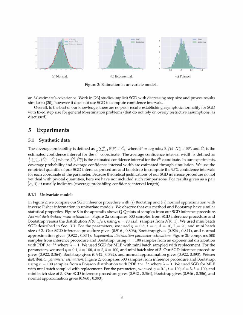
−1.00 −0.75 −0.50 −0.25 0.00 0.25 0.50 0.75 1.000.0
0.5
1.0
1.5
2.0
N(0, 1/n)
θSGD − θSGDθbootstrap − θbootstrap
(a) Normal.
0.8 1.0 1.2 1.4 1.60
1
2
3
4
SGDbootstrap
(b) Exponential.
0.8 1.0 1.2 1.40
1
2
3
4
5SGDbootstrap
(c) Poisson.
Figure 2: Estimation in univariate models.
an M -estimate’s covariance. Work in [23] studies implicit SGD with decreasing step size and proves resultssimilar to [20], however it does not use SGD to compute confidence intervals.
Overall, to the best of our knowledge, there are no prior results establishing asymptotic normality for SGDwith fixed step size for general M-estimation problems (that do not rely on overly restrictive assumptions, asdiscussed).
5 Experiments
5.1 Synthetic data
The coverage probability is defined as 1p
∑pi=1 P[θ?i ∈ Ci] where θ? = arg minθ E[f(θ,X)] ∈ Rp, and Ci is the
estimated confidence interval for the ith coordinate. The average confidence interval width is defined as1p
∑pi=1(Cui −Cli) where [Cli , C
ui ] is the estimated confidence interval for the ith coordinate. In our experiments,
coverage probability and average confidence interval width are estimated through simulation. We use theempirical quantile of our SGD inference procedure and bootstrap to compute the 95% confidence intervalsfor each coordinate of the parameter. Because theoretical justifications of our SGD inference procedure do notyet deal with pivotal quantities, here we have not included such comparisons. For results given as a pair(α, β), it usually indicates (coverage probability, confidence interval length).
5.1.1 Univariate models
In Figure 2, we compare our SGD inference procedure with (i) Bootstrap and (ii) normal approximation withinverse Fisher information in univariate models. We observe that our method and Bootstrap have similarstatistical properties. Figure 8 in the appendix shows Q-Q plots of samples from our SGD inference procedure.Normal distribution mean estimation: Figure 2a compares 500 samples from SGD inference procedure andBootstrap versus the distribution N (0, 1/n), using n = 20 i.i.d. samples from N (0, 1). We used mini batchSGD described in Sec. 3.3. For the parameters, we used η = 0.8, t = 5, d = 10, b = 20, and mini batchsize of 2. Our SGD inference procedure gives (0.916 , 0.806), Bootstrap gives (0.926 , 0.841), and normalapproximation gives (0.922 , 0.851). Exponential distribution parameter estimation: Figure 2b compares 500samples from inference procedure and Bootstrap, using n = 100 samples from an exponential distributionwith PDF λe−λx where λ = 1. We used SGD for MLE with mini batch sampled with replacement. For theparameters, we used η = 0.1, t = 100, d = 5, b = 100, and mini batch size of 5. Our SGD inference proceduregives (0.922, 0.364), Bootstrap gives (0.942 , 0.392), and normal approximation gives (0.922, 0.393). Poissondistribution parameter estimation: Figure 2c compares 500 samples from inference procedure and Bootstrap,using n = 100 samples from a Poisson distribution with PDF λxe−λx where λ = 1. We used SGD for MLEwith mini batch sampled with replacement. For the parameters, we used η = 0.1, t = 100, d = 5, b = 100, andmini batch size of 5. Our SGD inference procedure gives (0.942 , 0.364), Bootstrap gives (0.946 , 0.386), andnormal approximation gives (0.960 , 0.393).
8

η t = 100 t = 500 t = 2500
0.1 (0.957, 4.41) (0.955, 4.51) (0.960, 4.53)0.02 (0.869, 3.30) (0.923, 3.77) (0.918, 3.87)0.004 (0.634, 2.01) (0.862, 3.20) (0.916, 3.70)
(a) Bootstrap (0.941, 4.14), normal approximation (0.928, 3.87)
η t = 100 t = 500 t = 2500
0.1 (0.949, 4.74) (0.962, 4.91) (0.963, 4.94)0.02 (0.845, 3.37) (0.916, 4.01) (0.927, 4.17)0.004 (0.616, 2.00) (0.832, 3.30) (0.897, 3.93)
(b) Bootstrap (0.938, 4.47), normal approximation (0.925, 4.18)
Table 1: Linear regression. Left: Experiment 1, Right: Experiment 2.
η t = 100 t = 500 t = 2500
0.1 (0.872, 0.204) (0.937, 0.249) (0.939, 0.258)0.02 (0.610, 0.112) (0.871, 0.196) (0.926, 0.237)0.004 (0.312, 0.051) (0.596, 0.111) (0.86, 0.194)
(a) Bootstrap (0.932, 0.253), normal approximation (0.957, 0.264)
η t = 100 t = 500 t = 2500
0.1 (0.859, 0.206) (0.931, 0.255) (0.947, 0.266)0.02 (0.600, 0.112) (0.847, 0.197) (0.931, 0.244)0.004 (0.302, 0.051) (0.583, 0.111) (0.851, 0.195)
(b) Bootstrap (0.932, 0.245), normal approximation (0.954, 0.256)
Table 2: Logistic regression. Left: Experiment 1, Right: Experiment 2.
5.1.2 Multivariate models
In these experiments, we set d = 100, used mini-batch size of 4, and used 200 SGD samples. In all cases, wecompared with Bootstrap using 200 replicates. We computed the coverage probabilities using 500 simulations.Also, we denote 1p =
[1 1 . . . 1
]> ∈ Rp. Additional simulations comparing covariance matrix computedwith different methods are given in Sec. B.1.2.
Linear regression: Experiment 1: Results for the case where X ∼ N (0, I) ∈ R10, Y = w∗TX + ε, w∗ =1p/√p, and ε ∼ N (0, σ2 = 102) with n = 100 samples is given in Table 1a. Bootstrap gives (0.941, 4.14), and
confidence intervals computed using the error covariance and normal approximation gives (0.928, 3.87).Experiment 2: Results for the case where X ∼ N (0,Σ) ∈ R10, Σij = 0.3|i−j|, Y = w∗TX + ε, w∗ = 1p/
√p, and
ε ∼ N (0, σ2 = 102) with n = 100 samples is given in Table 1b. Bootstrap gives (0.938, 4.47), and confidenceintervals computed using the error covariance and normal approximation gives (0.925, 4.18).
Logistic regression: Here we show results for logistic regression trained using vanilla SGD with minibatch sampled with replacement. Results for modified SGD (Sec. 3.5) are given in Sec. B.1.2. Experiment 1:Results for the case where P[Y = +1] = P[Y = −1] = 1/2, X | Y ∼ N (0.01Y 1p/
√p, I) ∈ R10 with n = 1000
samples is given in Table 2a. Bootstrap gives (0.932, 0.245), and confidence intervals computed using inverseFisher matrix as the error covariance and normal approximation gives (0.954, 0.256). Experiment 2: Resultsfor the case where P[Y = +1] = P[Y = −1] = 1/2, X | Y ∼ N (0.01Y 1p/
√p,Σ) ∈ R10, Σij = 0.2|i−j| with
n = 1000 samples is given in Table 2b. Bootstrap gives (0.932, 0.253), and confidence intervals computedusing inverse Fisher matrix as the error covariance and normal approximation gives (0.957, 0.264).
5.2 Real data
Here, we compare covariance matrix computed using our SGD inference procedure, bootstrap, and inverseFisher information matrix on the Higgs data set [3] and the LIBSVM Splice data set, and we observe that theyhave similar statistical properties.
5.2.1 Higgs data set
The Higgs data set 3 [3] contains 28 distinct features with 11,000,000 data samples. This is a classificationproblem between two types of physical processes: one produces Higgs bosons and the other is a backgroundprocess that does not. We use a logistic regression model, trained using vanilla SGD, instead of the modifiedSGD described in Section 3.5.
3https://archive.ics.uci.edu/ml/datasets/HIGGS
9

0 5 10 15 20 25
0
5
10
15
20
25
7.5
6.0
4.5
3.0
1.5
0.0
1.5
3.0
4.5
6.0
7.5
(a) Inverse Fisher information
0 5 10 15 20 25
0
5
10
15
20
25
7.5
6.0
4.5
3.0
1.5
0.0
1.5
3.0
4.5
6.0
7.5
(b) SGD inference covariance
0 5 10 15 20 25
0
5
10
15
20
25
7.5
6.0
4.5
3.0
1.5
0.0
1.5
3.0
4.5
6.0
7.5
(c) Bootstrap estimated covariance
Figure 3: Higgs data set with n = 200
0 5 10 15 20 25
0
5
10
15
20
25
0.010
0.008
0.006
0.004
0.002
0.000
0.002
0.004
0.006
0.008
0.010
(a) Inverse Fisher information
0 5 10 15 20 25
0
5
10
15
20
25
0.010
0.008
0.006
0.004
0.002
0.000
0.002
0.004
0.006
0.008
0.010
(b) SGD inference covariance
Figure 4: Higgs data set with n = 50000
To understand different settings of sample size, we subsampled the data set with different samplesize levels: n = 200 and n = 50000. We investigate the empirical performance of SGD inference on thissubsampled data set. In all experiments below, the batch size of the mini batch SGD is 10.
In the case n = 200, the asymptotic normality for the MLE is not a good enough approximation. Hence,in this small-sample inference, we compare the SGD inference covariance matrix with the one obtained byinverse Fisher information matrix and bootstrap in Figure 3.
For our SGD inference procedure, we use t = 100 samples to average, and discard d = 50 samples. Weuse R = 20 averages from 20 segments (as in Figure 1). For bootstrap, we use 2000 replicates, which is muchlarger than the sample size n = 200.
Figure 3 shows that the covariance matrix obtained by SGD inference is comparable to the estimationgiven by bootstrap and inverse Fisher information.
In the case n = 50000, we use t = 5000 samples to average, and discard d = 500 samples. We use R = 20averages from 20 segments (as in Figure 1). For this large data set, we present the estimated covariance ofSGD inference procedure and inverse Fisher information (the asymptotic covariance) in Figure 4 becausebootstrap is computationally prohibitive. Similar to the small sample result in Figure 3, the covariance of ourSGD inference procedure is comparable to the inverse Fisher information.
In Figure 5, we compare the covariance matrix computed using our SGD inference procedure and inverseFisher information with n = 90000 samples . We used 25 samples from our SGD inference procedure witht = 5000, d = 1000, η = 0.2, and mini batch size of 10.
5.2.2 Splice data set
The Splice data set 4 contains 60 distinct features with 1000 data samples. This is a classification problembetween two classes of splice junctions in a DNA sequence. Similar to the Higgs data set, we use a logisticregression model, trained using vanilla SGD.
4https://www.csie.ntu.edu.tw/˜cjlin/libsvmtools/datasets/binary.html
10

0 5 10 15 20 25
0
5
10
15
20
25 0.004
0.002
0.000
0.002
0.004
(a) Inverse Fisher information
0 5 10 15 20 25
0
5
10
15
20
25 0.004
0.002
0.000
0.002
0.004
(b) SGD inference covariance
0 5 10 15 20 250.000
0.001
0.002
0.003
0.004SGD InferenceFisher
(c) Diagonal terms
Figure 5: Higgs data set with n = 90000
0 10 20 30 40 50 60
0
10
20
30
40
50
60
0.02
0.01
0.00
0.01
0.02
(a) Bootstrap
0 10 20 30 40 50 60
0
10
20
30
40
50
60
0.02
0.01
0.00
0.01
0.02
(b) SGD inference covariance
0 10 20 30 40 50 600.000
0.005
0.010
0.015
0.020
0.025
SGDbootstrap
(c) Diagonal terms
Figure 6: Splice data set
In Figure 6, we compare the covariance matrix computed using our SGD inference procedure andbootstrap n = 1000 samples. We used 10000 samples from both bootstrap and our SGD inference procedurewith t = 500, d = 100, η = 0.2, and mini batch size of 6.
0 5 10 15 20 25
0
5
10
15
20
25
(a) Original “0”: logit -46.3,CI (-64.2, -27.9)
0 5 10 15 20 25
0
5
10
15
20
25
(b) Adversarial “0”: logit 16.5,CI (-10.9, 30.5)
Figure 7: MNIST
5.2.3 MNIST
Here, we train a binary logistic regression classifier to classify 0/1 using perturbed MNIST data set, anddemonstrate that certain adversarial examples (e.g. [10]) can be detected using prediction confidence intervals.For each image, where each original pixel is either 0 or 1, we randomly changed 70% pixels to randomnumbers uniformly on [0, 0.9]. Figure 7 shows each image’s logit value (log
P[1|image]P[0|image] ) and its 95% confidence
interval (CI) computed using our SGD inference procedure.
11

5.3 Discussion
In our experiments, we observed that using a larger step size η produces accurate results with significantlyaccelerated convergence time. This might imply that the η term in Theorem 1’s bound is an artifact of ouranalysis. Indeed, although Theorem 1 only applies to SGD with fixed step size, where ηt→∞ and η2t→ 0imply that the step size should be smaller when the number of consecutive iterates used for the average islarger, our experiments suggest that we can use a (data dependent) constant step size η and only requireηt→∞.
In the experiments, our SGD inference procedure uses (t+ d) · S · p operations to produce a sample, andNewton method uses n·(matrix inversion complexity = Ω(p2))·(number of Newton iterations t) operationsto produce a sample. The experiments therefore suggest that our SGD inference procedure produces resultssimilar to Bootstrap while using far fewer operations.
12

References[1] F. Bach. Self-concordant analysis for logistic regression. Electronic Journal of Statistics, 4:384–414, 2010.
[2] F. Bach. Adaptivity of averaged stochastic gradient descent to local strong convexity for logistic regression. Journalof Machine Learning Research, 15(1):595–627, 2014.
[3] P. Baldi, P. Sadowski, and D. Whiteson. Searching for exotic particles in high-energy physics with deep learning.Nature Communications, 5, 2014.
[4] A. Benveniste, P. Priouret, and M. Metivier. Adaptive Algorithms and Stochastic Approximations. Springer-Verlag NewYork, Inc., New York, NY, USA, 1990.
[5] S. Bubeck. Convex optimization: Algorithms and complexity. Found. Trends Mach. Learn., 8(3-4):231–357, Nov. 2015.
[6] S. Bubeck, R. Eldan, and J. Lehec. Finite-time analysis of projected langevin monte carlo. In Advances in NeuralInformation Processing Systems, pages 1243–1251, 2015.
[7] X. Chen, J. Lee, X. Tong, and Y. Zhang. Statistical inference for model parameters in stochastic gradient descent.arXiv preprint arXiv:1610.08637, 2016.
[8] B. Efron. The jackknife, the bootstrap and other resampling plans. SIAM, 1982.
[9] B. Efron and R. Tibshirani. An introduction to the bootstrap. CRC press, 1994.
[10] I. Goodfellow, J. Shlens, and C. Szegedy. Explaining and harnessing adversarial examples. In International Conferenceon Learning Representations, 2015.
[11] R. Johnson and T. Zhang. Accelerating stochastic gradient descent using predictive variance reduction. In Advancesin Neural Information Processing Systems, pages 315–323, 2013.
[12] H. Kushner and H. Huang. Asymptotic properties of stochastic approximations with constant coefficients. SIAMJournal on Control and Optimization, 19(1):87–105, 1981.
[13] H. Kushner and G. Yin. Stochastic Approximation and Recursive Algorithms and Applications. Stochastic Modelling andApplied Probability. Springer New York, 2003.
[14] L. Ljung, G. C. Pflug, and H. Walk. Stochastic approximation and optimization of random systems, volume 17. Birkhauser,2012.
[15] S. Mandt, M. Hoffman, and D. Blei. A Variational Analysis of Stochastic Gradient Algorithms. In Proceedings of The33rd International Conference on Machine Learning, pages 354–363, 2016.
[16] S. Mandt, M. D. Hoffman, and D. M. Blei. Stochastic Gradient Descent as Approximate Bayesian Inference. arXivpreprint arXiv:1704.04289, 2017.
[17] D. Opitz and R. Maclin. Popular ensemble methods: An empirical study. Journal of Artificial Intelligence Research,11:169–198, 1999.
[18] G. Pflug. Stochastic minimization with constant step-size: asymptotic laws. SIAM Journal on Control and Optimization,24(4):655–666, 1986.
[19] D. Politis, J. Romano, and M. Wolf. Subsampling. Springer Series in Statistics. Springer New York, 2012.
[20] B. Polyak and A. Juditsky. Acceleration of stochastic approximation by averaging. SIAM Journal on Control andOptimization, 30(4):838–855, 1992.
[21] H. Robbins and S. Monro. A stochastic approximation method. The Annals of Mathematical Statistics, pages 400–407,1951.
[22] J. Shao and D. Tu. The jackknife and bootstrap. Springer Science & Business Media, 2012.
[23] P. Toulis and E. M. Airoldi. Asymptotic and finite-sample properties of estimators based on stochastic gradients.arXiv preprint arXiv:1408.2923, 2014.
13

[24] A. van der Vaart. Asymptotic Statistics. Cambridge Series in Statistical and Probabilistic Mathematics. CambridgeUniversity Press, 2000.
[25] L. Wasserman. All of statistics: a concise course in statistical inference. Springer Science & Business Media, 2013.
[26] M. Welling and Y. Teh. Bayesian learning via stochastic gradient Langevin dynamics. In Proceedings of the 28thInternational Conference on Machine Learning, pages 681–688, 2011.
14

A Proofs
A.1 Proof of Theorem 1
We first assume that θ1 = θ for more precise constants in our bounds, the same analysis applies when ‖θ1‖22For ease of notation, we denote
∆t = θt − θ, (14)
and, without loss of generality, we assume that θ = 0. The stochastic gradient descent recursion satisfies:
θt+1 = θt − η · gs(θt)= θt − η · (gs(θt)−∇f(θt) +∇f(θt))
= θt − η · ∇f(θt)− η · et,
where et = gs(θt)−∇f(θt). Note that e1, e2, . . . is a martingale difference sequence. We use
gi = ∇fi(θ) and Hi = ∇2fi(θ) (15)
to denote the gradient component at index i, and the Hessian component at index i, at optimum θ, respectively. Note that∑gi = 0 and 1
n
∑Hi = H .
For each fi, its Taylor expansion around θ is
fi(θ) = fi(θ) + g>i (θ − θ) +1
2(θ − θ)>Hi(θ − θ) +Ri(θ, θ), (16)
where Ri(θ, θ) is the remainder term. For convenience, we write R = 1n
∑Ri.
For the proof, we require the following lemmata. The following lemma states that E[‖∆t‖22] = O(η) as t→∞ and η → 0.
Lemma 1. For data dependent, positive constants α,A,B according to assumptions (F1) and (G2) in Theorem 1, and given assumption(G1), we have
E[‖∆t‖22
]≤ (1− 2αη +Aη2)t−1‖∆1‖22 +
Bη
2α−Aη , (17)
under the assumption η < 2αA .
Proof. As already stated, we assume without loss of generality that θ = 0. This further implies that: gs(θt) = gs(θt−θ) = gs(∆t),and
∆t+1 = ∆t − η · gs(∆t).
Given the above and assuming expectation E[·] w.r.t. the selection of a sample from Xini=1, we have:
E[‖∆t+1‖22 | ∆t
]= E
[‖∆t − ηgs(∆t)‖22 | ∆t
]= E
[‖∆t‖22 | ∆t
]+ η2 · E
[‖gs(∆t)‖22 | ∆t
]− 2η · E
[gs(∆t)
>∆t | ∆t
]= ‖∆t‖22 + η2 · E
[‖gs(∆t)‖22 | ∆t
]− 2η · ∇f(∆t)
>∆t
(i)
≤ ‖∆t‖22 + η2 ·(A · ‖∆t‖22 +B
)− 2η · α‖∆t‖22
= (1− 2αη +Aη2)‖∆t‖22 + η2B. (18)
15

where (i) is due to assumptions (F1) and (G2) of Theorem 1. Taking expectations for every step t = 1, · over the whole history,we obtain the recursion:
E[‖∆t+1‖22
]≤ (1− 2αη +Aη2)t−1‖∆1‖22 + η2B ·
t−1∑i=0
(1− 2αη +Aη2)i
= (1− 2αη +Aη2)t−1‖∆1‖22 + η2B · 1−(1−2αη+Aη2)t
2αη−Aη2
≤ (1− 2αη +Aη2)t−1‖∆1‖22 + ηB2α−Aη .
The following lemma states that E[‖∆t‖42] = O(η2) as t→∞ and η → 0.
Lemma 2. For data dependent, positive constants α,A,B,C,D according to assumptions (F1), (G1), (G2) in Theorem 1, we have:
E[‖∆t‖42] ≤(1− 4αη +A(6η2 + 2η3) +B(3η + η2) + C(2η3 + η4))t−1‖∆1‖42
+B(3η2 + η3) +D(2η2 + η3)
4α−A(6η + 2η2)−B(3 + η)− C(2η2 + η3). (19)
Proof. Given ∆t, we have the following sets of (in)equalities:
E[‖∆t+1‖42 | ∆t
]=E
[‖∆t − ηgs(∆t)‖42 | ∆t
]=E
[(‖∆t‖22 − 2η · gs(∆t)
>∆t + η2‖gs(∆t)‖22)2 | ∆t
]=E[‖∆t‖42 + 4η2(gs(∆t)
>∆t)2 + η4‖gs(∆t)‖42 − 4η · gs(∆t)
>∆t‖∆t‖22+ 2η2 · ‖gs(∆t)‖22‖∆t‖22 − 4η3 · gs(∆t)
>∆t‖gs(∆t)‖22 | ∆t
](i)
≤E[‖∆t‖42 + 4η2 · ‖gs(∆t)‖22 · ‖∆t‖22 + η4‖gs(∆t)‖42 − 4η · gs(∆t)
>∆t‖∆t‖22+ 2η2 · ‖gs(∆t)‖22 · ‖∆t‖22 + 2η3 · (‖gs(∆t)‖22 + ‖∆t‖22) · ‖gs(∆t)‖22 | ∆t
](ii)
≤ E[‖∆t‖42 + (2η3 + η4)‖gs(∆t)‖42 + (6η2 + 2η3)‖gs(∆t)‖22‖∆t‖22 | ∆t
]− 4αη‖∆t‖42
(iii)
≤ (1− 4αη)‖∆t‖42 + (6η2 + 2η3)(A‖∆t‖22 +B)‖∆t‖22 + (2η3 + η4)(C‖∆t‖42 +D)
=(1− 4αη +A(6η2 + 2η3) + C(2η3 + η4))‖∆t‖42 +B(6η2 + 2η3)‖∆t‖22 +D(2η3 + η4)
(iv)
≤ (1− 4αη +A(6η2 + 2η3) + C(2η3 + η4)) · ‖∆t‖42 +B(3η + η2)(η2 + ‖∆t‖42) +D(2η3 + η4)
=(1− 4αη +A(6η2 + 2η3) +B(3η + η2) + C(2η3 + η4)) · ‖∆t‖42 +Bη2(3η + η2) +D(2η3 + η4), (20)
where (i) is due to (gs(∆t)>∆t)
2 ≤ ‖gs(∆t)‖22 · ‖∆t‖22 and −2gs(∆t)>∆t ≤ ‖gs(∆t)‖22 + ‖∆t‖22, (ii) is due to assumptions (G1)
and (F1) in Theorem 1, (iii) is due to assumptions (G2) and (G3) in Theorem 1, and (iv) is due to 2η‖∆t‖22 ≤ η2 + ‖∆t‖42.Similar to the proof of the previous lemma, applying the above rule recursively and w.r.t. the whole history of estimates, we
16

obtain:
E[‖∆t+1‖42
]≤ (1− 4αη +A(6η2 + 2η3) +B(3η + η2) + C(2η3 + η4))t−1‖∆1‖42
+(Bη2(3η + η2) +D(2η3 + η4)
)·t−1∑i=0
(1− 4αη +A(6η2 + 2η3) +B(3η + η2) + C(2η3 + η4)
)i≤ (1− 4αη +A(6η2 + 2η3) +B(3η + η2) + C(2η3 + η4))t−1‖∆1‖42
+Bη2(3η + η2) +D(2η3 + η4)
4αη −A(6η2 + 2η3)−B(3η + η2)− C(2η3 + η4),
which is the target inequality, after simple transformations.
For SGD, we have
∆t = (I − ηH)∆t−1 − η(∇R(∆t−1) + et−1)
= (I − ηH)t−1∆1 − ηt−1∑i=1
(I − ηH)t−1−i(ei +∇R(∆i)). (21)
For t ≥ 2,
t(θ − θ) =
>∑i=1
∆i
= (I − (I − ηH)t)H−1
η∆1 − η
t−1∑j=1
j∑i=1
(I − ηH)j−1−i(ei +∇R(∆i)). (22)
For the latter term,
ηt−1∑j=1
j∑i=1
(I − ηH)j−i(ei +∇R(∆i))
=η
t−1∑i=1
(
t−i−1∑j=0
(I − ηH)j)(ei +∇R(∆i))
=t−1∑i=1
(I − (I − ηH)t−i)H−1(ei +∇R(∆i))
=H−1t−1∑i=1
ei +H−1t−1∑i=1
∇R(∆i)−H−1t−1∑i=1
(I − ηH)t−i(ei +∇R(∆i))
(i)=H−1
t−1∑i=1
ei +H−1t−1∑i=1
∇R(∆i) +H−1(I − ηH)1
η(∆t − (I − ηH)t−1∆1), (23)
where step (i) follows from the fact∑t−1i=1(I − ηH)t−i(ei +∇R(∆i)) = (I − ηH) 1
η (∆t − (I − ηH)t−1∆1) .
17

Thus, we have
√t∆t =
1√t(I − (I − ηH)t)
H−1
η∆1
− 1√tH−1
t−1∑i=1
ei
− 1√tH−1
t−1∑i=1
∇R(∆i)
− 1√tH−1(I − ηH)
1
η(∆t − (I − ηH)t−1∆1). (24)
In the statement of the theorem we have ∆1 = 0 (however similar bounds will hold if ‖∆1‖22 = O(η)), thus for above termswe have
1√t(I − (I − ηH)t)
H−1
η∆1 = 0, (25)
E[‖ 1√tH−1(I − ηH)
1
η(∆t − (I − ηH)t−1∆1)‖22]
≤1− ηλUλL
E[‖∆t‖22η2t
]
≤1− ηλUλL
1
η2t((1− 2αη +Aη2)t−1‖∆1‖22 +
Bη
2α−Aη )
≤1− ηλUλL
B
tη(2α−Aη)
=O(1
tη). (26)
18

E[‖ 1√tH−1
t−1∑i=1
∇R(∆i)‖22]
≤E[1
λL
1
t(t−1∑i=1
‖∇R(∆i)‖2)2]
≤E[E2
λLt(t−1∑i=1
‖∆i‖22)2]
≤ E2
λLt(t− 1)E[
t−1∑i=1
‖∆i‖42]
≤E2
λL
t
t− 1
t−1∑i=1
((1− 4αη +A(6η2 + 2η3) + C(2η3 + η4))t−1‖∆1‖42 +B(3η2 + η3) +D(2η2 + η3)
4α−A(6η + 2η2)− C(2η2 + η3))
=E2
λLt
B(3η2 + η3) +D(2η2 + η3)
4α−A(6η + 2η2)− C(2η2 + η3)
=O(tη2). (27)
For the term − 1√tH−1
∑t−1i=1 ei, we have
E[‖ − 1√tH−1
t−1∑i=1
ei‖22]
(i)=
1
t
t−1∑i=1
E[‖H−1ei‖22]
≤λUt
t−1∑i=1
E[‖ei‖22]
=λUt
t−1∑i=1
E[‖gs(∆i)−∇f(∆i)‖22]
≤2λUt
(
t−1∑i=1
E[‖gs(∆i)‖22] +
t−1∑i=1
E[‖∇f(∆i)‖22])
≤2λUt
((t− 1)B + (A+ L2)t−1∑i=1
‖∆i‖22)
≤2λUt
((t− 1)B + (A+ L2)t−1∑i=1
((1− 2αη +Aη2)t−1‖∆1‖22 +Bη
2α−Aη ))
=2λUt− 1
t(B + (A+ L2)
Bη
2α−Aη )
=O(1), (28)
19

where step (i) follows from i 6= j leading to E[(H−1ei)>H−1ej ] = 0. We also have
E[(− 1√tH−1
t−1∑i=1
ei)(−1√tH−1
t−1∑i=1
ei)>]
=1
tH−1(
t−1∑i=1
E[eie>i ])H−1. (29)
For each term E[eie>i ], we have
‖E[eie>i ]−G‖2
=‖E[gs(∆i)gs(∆i)>]− E[(∇f(∆i))(∇f(∆i))
>]−G‖2≤E[‖∇f(∆i)‖22] + E[A1‖∆i‖2 +A2‖∆i‖22 +A3‖∆i‖32 +A4‖∆i‖42]
≤L2E[‖∆i‖22] +A1
√E[‖∆i‖22] +A2E[‖∆i‖22] +
A3
2E[‖∆i‖22 + ‖∆i‖42] +A4E[‖∆i‖42]
=A1
√E[‖∆i‖22] + (L2 +A2 +
A3
2)E[‖∆i‖22] + (
A3
2+A4)E[‖∆i‖42]
≤A1
√(1− 2αη +Aη2)t−1‖∆1‖22 +
Bη
2α−Aη + (L2 +A2 +A3
2)((1− 2αη +Aη2)t−1‖∆1‖22 +
Bη
2α−Aη )
+ (A3
2+A4)((1− 4αη +A(6η2 + 2η3) + C(2η3 + η4))t−1‖∆1‖42 +
B(3η2 + η3) +D(2η2 + η3)
4α−A(6η + 2η2)− C(2η2 + η3))
=A1
√Bη
2α−Aη + (L2 +A2 +A3
2)
Bη
2α−Aη + (A3
2+A4)
B(3η2 + η3) +D(2η2 + η3)
4α−A(6η + 2η2)− C(2η2 + η3). (30)
Thus, we have
‖1
tH−1(
t−1∑i=1
E[eie>i ])H−1 −H−1GH−1‖2
≤1
t‖H−1GH−1‖2
+t− 1
t
1
λ2L
(A1
√Bη
2α−Aη + (L2 +A2 +A3
2)
Bη
2α−Aη + (A3
2+A4)
B(3η2 + η3) +D(2η2 + η3)
4α−A(6η + 2η2)− C(2η2 + η3))
=O(√η). (31)
20

For convenience, denote
0 =1√t(I − (I − ηH)t)
H−1
η∆1,
1 = − 1√tH−1(I − ηH)
1
η(∆t − (I − ηH)t−1∆1),
2 = − 1√tH−1
t−1∑i=1
∇R(∆i),
3 = − 1√tH−1
t−1∑i=1
ei, (32)
and we have E[t∆t∆t] = E[(0 +1 +2 +3)(0 +1 +2 +3)>].Combining above results, we can bound
‖tE[(θt − θ)(θt − θ)>]−H−1GH−1‖2=‖E[(0 +1 +2 +3)(0 +1 +2 +3)>]−H−1GH−1‖2=‖E[3
>3 ]−H−1GH−1 + E[3(0 +1 +2)> + (0 +1 +2)>3 + (0 +1 +2)(0 +1 +2)>]‖2
.‖E[3>3 ]−H−1GH−1‖2 +
√E[‖3‖22](E[‖0‖22] + E[‖1‖22] + E[‖2‖22]) + E[‖0‖22] + E[‖1‖22] + E[‖2‖22]
.√η +
√1
tη+ tη2. (33)
Here we have used the fact that for two p-dimensional random vectors a and b, the expectation of the matrix ab> satisfies
‖E[ab>]‖2 ≤√
E[‖a‖22]E[‖b‖22] ≤ 1
2E[‖a‖22] + E[‖b‖22]. (34)
Indeed, for any fixed unit vector u we have ‖E[ab>]u‖2 = ‖E[a(b>u)]‖2 ≤ E[‖a‖2|b>u|] ≤ E[‖a‖2‖b‖2] ≤√E[‖a‖22]E[‖b‖22].
Here we used the fact ‖E[x]‖2 ≤ E[‖x‖2] because ‖x‖2 is convex.
A.2 Proof of Corollary 1
Proof of Corollary 1. Here we use the same notations as the proof of Theorem 1.Because linear regression satisfies ∇f(θ) −H(θ − θ) = 0, we do not have to consider the Taylor remainder term in our
analysis. And we do not need 4-th order bound for SGD.Because the quadratic function is strongly convex, we have ∆>∇f(∆ + θ) ≥ λL‖∆‖22.
21

By sampling with replacement, we have
E[‖gs(θt)‖22 | θt]=‖∇f(θt)‖22 + E[‖et‖22 | θt]
=‖∇f(θt)‖22 +1
S(
1
n
∑‖∇fi(θt)‖22 − ‖∇f(θt)‖22)
≤L2(1− 1
S)‖∆t‖22 +
1
S
1
n
∑‖xi(x>i θt − yi)‖22
=L2(1− 1
S)‖∆t‖22 +
1
S
1
n
∑‖xix>i ∆t + xix
>i θ − yixi‖22
≤L2(1− 1
S)‖∆t‖22 + 2
1
S
1
n
∑(‖xix>i ∆t‖22 + ‖xix>i θ − yixi‖22)
≤(L2(1− 1
S) + 2
1
S
1
n
∑‖xi‖42)‖∆t‖22 + 2
1
S
1
n
∑‖xix>i θ − yixi‖22. (35)
We also have
‖E[gs(θ)gs(θ)> | θ]−G‖2
=‖ 1
S
1
n
∑∇fi(θ)fi(θ)> −∇f(θ)∇f(θ)> −G‖2
≤‖∇f(θ)‖22 +1
S‖ 1
n
∑∇fi(θ)fi(θ)> −G‖2
≤‖∇f(θ)‖22 +1
S‖ 1
n
∑(gi +Hi∆)(gi +Hi∆)> −G‖2
≤‖∇f(θ)‖22 +1
S‖ 1
n
∑Hi∆g
>i + gi∆
>Hi +Hi∆∆>Hi‖2
≤‖∇f(θ)‖22 +1
S(
2
n‖Hi‖2‖gi‖2)‖∆‖2 +
1
S(
1
n
∑‖Hi‖22)‖∆‖22
≤ 1
S(
2
n‖Hi‖2‖gi‖2)‖∆‖2 + (L2 +
1
S
1
n
∑‖Hi‖22)‖∆‖22, (36)
where gi = xi(x>i θ − yi) and Hi = xix
>i .
Following Theorem 1’s proof, we have
‖tE[(θt − θ)(θt − θ)>]−H−1GH−1‖2 .√η +
1√tη. (37)
A.3 Proof of Corollary 2
Proof of Corollary 2. Here we use the same notations as the proof of Theorem 1.Because∇2f(θ) = ∇k(θ)∇k(θ)> + (k(θ) + c)∇2k(θ), f(θ) is convex.The following lemma shows that∇f(θ) = (k(θ) + c)∇k(θ) is Lipschitz.
Lemma 3.
‖∇f(θ)‖2 ≤ L‖∆‖2 (38)
for some data dependent constant L.
22

Proof. First, because
∇k(θ) =1
n
∑− −yixi
1 + exp(yiθ>xi), (39)
we have
‖∇k(θ)‖2 ≤1
n
∑‖xi‖2. (40)
Also, we have
‖∇2k(θ)‖2 =‖ 1
n
∑ exp(yiθ>xi)
(1 + exp(yiθ>xi))2xix>i ‖2
≤ 1
4
1
n
∑‖xi‖22, (41)
which implies
‖∇k(θ)‖2 ≤1
4
1
n
∑‖xi‖22‖∆‖2. (42)
And, we have
k(θ) =1
n
∑log(1 + exp(−yi∆>xi − yiθ>xi))
≤ 1
n
∑log(1 + exp(‖xi‖2‖∆‖2 − yiθ>xi))
(i)
≤ 1
n
∑(log(1 + exp(−yiθ>xi)) + ‖xi‖2‖∆‖2) (43)
where step (i) follows from log(1 + exp(a+ b)) ≤ log(1 + eb) + |a|. Thus, we have
‖∇f(θ)‖2=‖(k(θ) + c)∇k(θ)‖2≤k(θ)‖∇k(θ)‖2 + c‖∇k(θ)‖2≤(c+
1
n
∑log(1 + exp(−yiθ>xi)))‖∇k(θ)‖2 + (
1
n
∑‖xi‖2)2‖∆‖2, (44)
and we can conclude that ‖∇f(θ)‖2 ≤ L‖∆‖2 for some data dependent constant L.
Next, we show that f(θ) has a bounded Taylor remainder.
Lemma 4.
‖∇f(θ)−H(θ − θ)‖2 ≤ E‖θ − θ‖22, (45)
for some data dependent constant E.
23

Proof. Because∇f(θ) = (k(θ) + c)∇k(θ), we know that ‖∇f(θ)‖2 = O(‖∆‖2) when ‖∆‖2 = Ω(1) where the constants are datadependent.
Because f(θ) is infinitely differentiable, by the Taylor expansion we know that ‖∇f(θ)−H(θ − θ)‖2 = O(‖θ − θ‖22) when‖∆‖2 = O(1) where the constants are data dependent.
Combining the above, we can conclude ‖∇f(θ)−H(θ − θ)‖2 ≤ E‖θ − θ‖22 for some data dependent constant E.
In the following lemma, we will show that∇f(θ)>(θ − θ) ≥ α‖θ − θ‖22 for some data dependent constant α.
Lemma 5.
∇f(θ)>(θ − θ) ≥ α‖θ − θ‖22, (46)
for some data dependent constant α.
Proof.
∇f(θ)>∆ = (k(θ) + c)∇k(θ)>∆. (47)
First, notice that locally (when ‖∆‖2 = O(λL
E )) we have
∇k(θ)>∆ & ∆>H∆ & λL‖∆‖22, (48)
because of the optimality condition. This lower bounds ∇f(θ)>(θ − θ) when ‖∆‖2 = O(λL
E ). Next we will lower bound itwhen ‖∆‖2 = Ω(λL
E ).Consider the function for t ∈ [0,∞), we have
g(t) = ∇f(θ + ut)>ut
= (k(θ + ut) + c)∇k(θ + ut)>ut
= k(θ + ut)∇k(θ + ut)>ut+ c∇k(θ + ut)>ut, (49)
where u = ∆‖∆‖2 .
Because k(θ) is convex,∇k(θ + ut)>u is an increasing function in t, thus we have∇k(θ + ut)>u = Ω(λ2L
E ) when t = Ω(λL
E ).
And we can deduce∇k(θ + ut)>ut = Ω(λ2L
E t) when t = Ω(λL
E ).
Similarly, because k(θ) is convex, k(θ + ut) is an increasing function in t. Its derivative ∇k(θ + ut)>u = Ω(λ2L
E ) when
t = Ω(λL
E ). So we have k(θ + ut) = Ω(λ2L
E t) when t = Ω(λL
E ).Thus, we have
k(θ + ut)∇k(θ + ut)>ut = Ω(λ4L
E2t2), (50)
when t = Ω( EλL).
And we can conclude that∇f(θ)>(θ − θ) ≥ α‖θ − θ‖22 for some data dependent constant α = Ω(minλL, λ4L
E2 ).
24

Next, we will prove properties about gs = ΨsΥs.
E[‖Υ‖22 | θ] =1
SΥ(
1
n
∑‖∇ki(θ)‖22 − ‖∇k(θ)‖22) + ‖∇k(θ)‖22
.1
n‖xi‖22 (51)
E[Ψ2s]
(i)
≤ 1
n
∑(c+ ki(θ))
2
=1
n
∑(c+ log(1 + exp(−yiθ>xi − yi∆xi)))2
(ii)
.1
n
∑‖xi‖2‖∆‖22 +
1
n
∑(c+ log(1 + exp(−yiθ>xi)))2, (52)
where (i) follows from E[(∑S
j=1 Xj
S )2] ≤ E[∑S
j=1 X2j
S ] and (ii) follows from log(1 + exp(a+ b)) ≤ log(1 + eb) + |a|.Thus we have
E[‖gs‖22(θ) | θ]=E[Ψ2 | θ]E[‖Υ‖22 | θ].A‖∆‖22 +B (53)
for some data dependent constants A and B.
E[‖Υ‖42 | θ]
=E[‖ 1
SΥ
∑i∈IΥ
t
∇ log(1 + exp(−yiθ>xi))‖42]
≤E[(1
SΥ
∑i∈IΥ
t
‖∇ log(1 + exp(−yiθ>xi))‖2)4]
≤E[(1
SΥ
∑i∈IΥ
t
‖xi‖2)4]
≤ 1
n
∑‖xi‖42. (54)
E[Ψ4s]
(i)
≤ 1
n
∑(c+ ki(θ))
4
=1
n
∑(c+ log(1 + exp(−yiθ>xi − yi∆xi)))4
(ii)
.1
n
∑‖xi‖4‖∆‖42 +
1
n
∑(c+ log(1 + exp(−yiθ>xi)))4, (55)
25

where (i) follows from E[(∑S
j=1 Xj
S )4] ≤ E[∑S
j=1 X4j
S ] and (ii) follows from log(1 + exp(a+ b)) ≤ log(1 + eb) + |a|.Thus we have
E[‖gs‖42(θ) | θ]=E[Ψ4 | θ]E[‖Υ‖42 | θ].C‖∆‖42 +D, (56)
for some data dependent constants C and D.
‖E[∇gs(θ)∇gs(θ)>]−G‖2≤‖KG(θ)
1
n
∑∇ki(θ)∇ki(θ)> −KG(θ)
1
n
∑∇ki(θ)∇ki(θ)>‖2
≤‖KG(θ)1
n
∑∇ki(θ)∇ki(θ)> −KG(θ)
1
n
∑∇ki(θ)∇ki(θ)> +KG(θ)
1
n
∑∇ki(θ)∇ki(θ)> −KG(θ)
1
n
∑∇ki(θ)∇ki(θ)>‖2
≤KG(θ)1
n‖∑
(∇ki(θ)∇ki(θ)> −∇ki(θ)∇ki(θ)>)‖2 + |KG(θ)−KG(θ)|‖ 1
n
∑∇ki(θ)∇ki(θ)>‖2. (57)
Because
KG(θ) = O(1 + ‖∆‖2 + ‖∆‖22), (58)1
n‖∑
(∇ki(θ)∇ki(θ)> −∇ki(θ)∇ki(θ)>)‖2 = O(‖∆‖2 + ‖∆‖22), (59)
|KG(θ)−KG(θ)| = O(‖∆‖2 + ‖∆‖22), (60)
where we have data dependent constants.Then, we have
‖E[gs(θ)gs(θ)> | θ]−G‖2 ≤ A1‖θ − θ‖2 +A2‖θ − θ‖22 +A3‖θ − θ‖32 +A4‖θ − θ‖42, (61)
for some data dependent constants A1, A2, A3, and A4.Combining above results and using Theorem 1, we have
‖tE[(θt − θ)(θt − θ)>]−H−1GH−1‖2
.√η +
√1
tη+ tη2. (62)
B Experiments
Here we present additional experiments on our SGD inference procedure.
B.1 Synthetic data
B.1.1 Univariate models
Figure 8 shows Q-Q plots for samples shown in Figure 2.
26

3 2 1 0 1 2 3Theoretical Quantiles
0.4
0.2
0.0
0.2
0.4
0.6
Sam
ple
Qua
ntile
s
(a) Normal.
3 2 1 0 1 2 3Theoretical Quantiles
0.9
1.0
1.1
1.2
1.3
1.4
1.5
Sam
ple
Qua
ntile
s(b) Exponential.
3 2 1 0 1 2 3Theoretical Quantiles
0.8
0.9
1.0
1.1
1.2
1.3
1.4
Sam
ple
Qua
ntile
s
(c) Poisson.
Figure 8: Estimation in univariate models: Q-Q plots for samples shown in Figure 2
B.1.2 Multivariate models
Here we show Q-Q plots per coordinate for samples from our SGD inference procedure.Q-Q plots per coordinate for samples in linear regression experiment 1 is shown in Figure 9. Q-Q plots per coordinate for
samples in linear regression experiment 2 is shown in Figure 10.
2 1 0 1 2Theoretical Quantiles
3
2
1
0
1
2
Sam
ple
Qua
ntile
s
2 1 0 1 2Theoretical Quantiles
2
1
0
1
2
3
Sam
ple
Qua
ntile
s
2 1 0 1 2Theoretical Quantiles
3
2
1
0
1
2
3
4
Sam
ple
Qua
ntile
s
2 1 0 1 2Theoretical Quantiles
2
1
0
1
2
3
4
Sam
ple
Qua
ntile
s
2 1 0 1 2Theoretical Quantiles
1
0
1
2
3
4
5
Sam
ple
Qua
ntile
s
2 1 0 1 2Theoretical Quantiles
1
0
1
2
3
4
5
6
Sam
ple
Qua
ntile
s
2 1 0 1 2Theoretical Quantiles
3
2
1
0
1
2
3
4
Sam
ple
Qua
ntile
s
2 1 0 1 2Theoretical Quantiles
3
2
1
0
1
2
3
Sam
ple
Qua
ntile
s
2 1 0 1 2Theoretical Quantiles
3
2
1
0
1
Sam
ple
Qua
ntile
s
2 1 0 1 2Theoretical Quantiles
2
1
0
1
2
3
4
Sam
ple
Qua
ntile
s
Figure 9: Linear regression experiment 1: Q-Q plots per coordinate
Q-Q plots per coordinate for samples in logistic regression experiment 1 is shown in Figure 11. Q-Q plots per coordinatefor samples in logistic regression experiment 2 is shown in Figure 12.
Additional experiments2-Dimensional Linear Regression. Consider:
y = x1 + x2 + ε, where[x1
x2
]∼ N
(0,
[1 0.8
0.8 1
])and ε ∼ N (0, σ2 = 102).
Each sample consists of Y = y and X = [x1, x2]>. We use linear regression to estimate w1, w2 in y = w1x1 + w2x2. In thiscase, the minimizer of the population least square risk is w?1 = 1, w?2 = 1.
27

2 1 0 1 2Theoretical Quantiles
0
2
4
6
Sam
ple
Qua
ntile
s
2 1 0 1 2Theoretical Quantiles
4
2
0
2
Sam
ple
Qua
ntile
s
2 1 0 1 2Theoretical Quantiles
2
1
0
1
2
3
Sam
ple
Qua
ntile
s
2 1 0 1 2Theoretical Quantiles
4
3
2
1
0
1
2
3
Sam
ple
Qua
ntile
s
2 1 0 1 2Theoretical Quantiles
6
4
2
0
2
4
Sam
ple
Qua
ntile
s
2 1 0 1 2Theoretical Quantiles
5
4
3
2
1
0
1
2
Sam
ple
Qua
ntile
s
2 1 0 1 2Theoretical Quantiles
6
4
2
0
2
4
Sam
ple
Qua
ntile
s
2 1 0 1 2Theoretical Quantiles
4
3
2
1
0
1
2
3
Sam
ple
Qua
ntile
s
2 1 0 1 2Theoretical Quantiles
3
2
1
0
1
2
Sam
ple
Qua
ntile
s
2 1 0 1 2Theoretical Quantiles
3
2
1
0
1
2
3
Sam
ple
Qua
ntile
s
Figure 10: Linear regression experiment 2: Q-Q plots per coordinate
2 1 0 1 2Theoretical Quantiles
0.15
0.10
0.05
0.00
0.05
0.10
0.15
0.20
Sam
ple
Qua
ntile
s
2 1 0 1 2Theoretical Quantiles
0.20
0.15
0.10
0.05
0.00
0.05
0.10
Sam
ple
Qua
ntile
s
2 1 0 1 2Theoretical Quantiles
0.15
0.10
0.05
0.00
0.05
0.10
0.15
0.20
Sam
ple
Qua
ntile
s
2 1 0 1 2Theoretical Quantiles
0.15
0.10
0.05
0.00
0.05
0.10
Sam
ple
Qua
ntile
s
2 1 0 1 2Theoretical Quantiles
0.15
0.10
0.05
0.00
0.05
0.10
Sam
ple
Qua
ntile
s
2 1 0 1 2Theoretical Quantiles
0.15
0.10
0.05
0.00
0.05
0.10
0.15
0.20
Sam
ple
Qua
ntile
s
2 1 0 1 2Theoretical Quantiles
0.20
0.15
0.10
0.05
0.00
0.05
0.10
Sam
ple
Qua
ntile
s
2 1 0 1 2Theoretical Quantiles
0.2
0.1
0.0
0.1
0.2
Sam
ple
Qua
ntile
s
2 1 0 1 2Theoretical Quantiles
0.10
0.05
0.00
0.05
0.10
0.15
0.20
Sam
ple
Qua
ntile
s
2 1 0 1 2Theoretical Quantiles
0.15
0.10
0.05
0.00
0.05
0.10
0.15
Sam
ple
Qua
ntile
s
Figure 11: Logistic regression experiment 1: Q-Q plots per coordinate
For 300 i.i.d. samples, we plotted 100 samples from SGD inference in Figure 13. We compare our SGD inference procedureagainst bootstrap in Figure 13a. Figure 13b and Figure 13c show samples from our SGD inference procedure with differentparameters.
10-Dimensional Linear Regression.Here we consider the following model
y = x>w? + ε,
where w? = 1√10
[1, 1, · · · , 1]> ∈ R10, x ∼ N (0,Σ) with Σij = 0.8|i−j|, and ε ∼ N (0, σ2 = 202), and use n = 1000 samples.We estimate the parameter using
w = argminw
1
n
n∑i=1
12 (x>i w − yi)2.
Figure 14 shows the diagonal terms of of the covariance matrix computed using the sandwich estimator and our SGDinference procedure with different parameters. 100000 samples from our SGD inference procedure are used to reduce theeffect of randomness.
28

2 1 0 1 2Theoretical Quantiles
0.2
0.1
0.0
0.1
0.2
Sam
ple
Qua
ntile
s
2 1 0 1 2Theoretical Quantiles
0.15
0.10
0.05
0.00
0.05
0.10
0.15
Sam
ple
Qua
ntile
s
2 1 0 1 2Theoretical Quantiles
0.1
0.0
0.1
0.2
Sam
ple
Qua
ntile
s
2 1 0 1 2Theoretical Quantiles
0.20
0.15
0.10
0.05
0.00
0.05
0.10
Sam
ple
Qua
ntile
s
2 1 0 1 2Theoretical Quantiles
0.15
0.10
0.05
0.00
0.05
0.10
0.15
0.20
Sam
ple
Qua
ntile
s
2 1 0 1 2Theoretical Quantiles
0.1
0.0
0.1
0.2
Sam
ple
Qua
ntile
s
2 1 0 1 2Theoretical Quantiles
0.1
0.0
0.1
0.2
Sam
ple
Qua
ntile
s
2 1 0 1 2Theoretical Quantiles
0.2
0.1
0.0
0.1
Sam
ple
Qua
ntile
s
2 1 0 1 2Theoretical Quantiles
0.1
0.0
0.1
0.2
0.3
Sam
ple
Qua
ntile
s
2 1 0 1 2Theoretical Quantiles
0.15
0.10
0.05
0.00
0.05
0.10
0.15
0.20
Sam
ple
Qua
ntile
s
Figure 12: Logistic regression experiment 2: Q-Q plots per coordinate
2-Dimensional Logistic Regression.Here we consider the following model
P[Y = +1] = P[Y = −1] =1
2, X | Y ∼ N
(µ = 1.1 + 0.1Y, σ2 = 1
). (63)
We use logistic regression to estimate w, b in the classifier sign(wx+ b) where the minimizer of the population logistic risk isw? = 0.2, b? = −0.22.
For 100 i.i.d. samples, we plot 1000 samples from SGD in Figure 15. In our simulations, we notice that our modifiedSGD for logistic regression behaves similar to vanilla logistic regression. T his suggests that an assumption weaker than(θ − θ)>∇f(θ) ≥ α‖θ − θ‖22 (assumption (F1) in Theorem 1) is sufficient for SGD analysis. Figure 15b and Figure 15d suggestthat the tη2 term in Corollary 2 is an artifact of our analysis, and can be improved.
11-Dimensional Logistic Regression.Here we consider the following model
P[Y = +1] = P[Y = −1] =1
2, X | Y ∼ N (0.01Y µ,Σ) ,
2 1 0 1 2 3w1
2
1
0
1
2
3
4
w2
bootstrapSGD
(a) SGD inference vs. bootstrap
2 1 0 1 2 3w1
2
1
0
1
2
3
4
w2
= .1 = .05 = .025 = .0125
(b) t = 800
2 1 0 1 2 3w1
2
1
0
1
2
3
4
w2
t = 100t = 200t = 400t = 400
(c) η = 0.1
Figure 13: 2-dimensional linear regression
29

0 2 4 6 80.0
0.5
1.0
1.5
2.0
2.5
3.0
sandwich= 0.05= 0.01= 0.002
(a) t = 500
0 2 4 6 80.0
0.5
1.0
1.5
2.0
2.5
3.0
sandwich= 0.05= 0.01= 0.002
(b) t = 2500
0 2 4 6 80.0
0.5
1.0
1.5
2.0
2.5
3.0
sandwich= 0.05= 0.01= 0.002
(c) t = 12500
0 2 4 6 80.0
0.5
1.0
1.5
2.0
2.5
3.0
sandwicht = 12500t = 2500t = 500
(d) η = 0.05
0 2 4 6 80.0
0.5
1.0
1.5
2.0
2.5
3.0
sandwicht = 12500t = 2500t = 500
(e) η = 0.01
0 2 4 6 80.0
0.5
1.0
1.5
2.0
2.5
3.0
sandwicht = 12500t = 2500t = 500
(f) η = 0.002
Figure 14: 11-dimensional linear regression: covariance matrix diagonal terms of SGD inference and sandwich estimator
30

2.0 1.5 1.0 0.5 0.0 0.5 1.0 1.5 2.0w
2.0
1.5
1.0
0.5
0.0
0.5
1.0
1.5
2.0
b
bootstrapSGD
(a) Modified SGD with t = 1000 and η = 0.1
2.0 1.5 1.0 0.5 0.0 0.5 1.0 1.5 2.0w
2
1
0
1
2
3
b
t = 1000t = 10000t = 100000
(b) Modified SGD with η = 0.1
1.5 1.0 0.5 0.0 0.5 1.0w
1.0
0.5
0.0
0.5
1.0
1.5
2.0
2.5
b
bootstrapSGD
(c) Vanilla SGD with t = 1000 and η = 0.1
2 1 0 1 2w
3
2
1
0
1
2
3
4
b
t = 1000t = 10000t = 100000
(d) Vanilla SGD with η = 0.1
0.8 0.6 0.4 0.2 0.0 0.2 0.4w
0.5
0.0
0.5
1.0
1.5
b
modified SGDvanilla SGD
(e) t = 1000 and η = 0.1
Figure 15: 2-dimensional logistic regression
where Σii = 1 and when i 6= j Σij = ρ|i−j| for some ρ ∈ [0, 1), and µ = 1√10
[1, 1, · · · , 1]> ∈ R10. We estimate a classifiersign(w>x+ b) using
w, b = argminw,b
1
n
n∑i=1
log(1 + exp(−Yi(w>Xi + b))
). (64)
Figure 16 shows results for ρ = 0 with n = 80 samples. We use t = 100, d = 70, η = 0.8, and mini batch of size 4 in vanillaSGD. Bootstrap and our SGD inference procedure each generated 2000 samples. In bootstrap, we used Newton method toperform optimization over each replicate, and 6-7 iterations were used. In figure 17, we follow the same procedure for ρ = 0.6with n = 80 samples. Here, we use t = 200, d = 70, η = 0.85; the rest of the setting is the same.
B.2 Real Data
B.2.1 MNIST
Here, we train a binary logistic regression classifier to classify 0/1 using perturbed MNIST data set, and demonstrate thatcertain adversarial examples (e.g. [10]) can be detected using prediction confidence intervals. For each image, where eachoriginal pixel is either 0 or 1, we randomly changed 70% pixels to random numbers uniformly on [0, 0.9]. Figure 18 shows
31

0 2 4 6 8 10
0
2
4
6
8
100.20
0.15
0.10
0.05
0.00
0.05
0.10
0.15
0.20
(a) SGD covariance
0 2 4 6 8 10
0
2
4
6
8
100.20
0.15
0.10
0.05
0.00
0.05
0.10
0.15
0.20
(b) Bootstrap estimated covariance
0 2 4 6 8 100.000
0.025
0.050
0.075
0.100
0.125
0.150
0.175
0.200
SGDbootstrap
(c) Diagonal terms
Figure 16: 11-dimensional logistic regression: ρ = 0
0 2 4 6 8 10
0
2
4
6
8
100.4
0.3
0.2
0.1
0.0
0.1
0.2
0.3
0.4
(a) SGD covariance
0 2 4 6 8 10
0
2
4
6
8
100.4
0.3
0.2
0.1
0.0
0.1
0.2
0.3
0.4
(b) Bootstrap estimated covariance
0 2 4 6 8 100.00
0.05
0.10
0.15
0.20
0.25
0.30
0.35
0.40
SGDbootstrap
(c) Diagonal terms
Figure 17: 11-dimensional logistic regression: ρ = 0.6
32

each image’s logit value (logP[1|image]P[0|image] ) and its 95% confidence interval computed using our SGD inference procedure. The
adversarial perturbation used here is shown in Figure 19 (scaled for display).
0 5 10 15 20 25
0
5
10
15
20
25
(a) Original “0”: logit -72.6,CI (-106.4, -30.0)
0 5 10 15 20 25
0
5
10
15
20
25
(b) Adversarial “0”: logit 15.3,CI (-6.5, 26.2)
0 5 10 15 20 25
0
5
10
15
20
25
(c) Original “0”: logit -62.1,CI (-101.6, -5.5)
0 5 10 15 20 25
0
5
10
15
20
25
(d) Adversarial “0”: logit 1.9,CI (-4.9, 11.6)
0 5 10 15 20 25
0
5
10
15
20
25
(e) Original “0”: logit -42.9,CI (-75.4, 5.1)
0 5 10 15 20 25
0
5
10
15
20
25
(f) Adversarial “0”: logit 4.8,CI (-3.4, 17.9)
0 5 10 15 20 25
0
5
10
15
20
25
(g) Original “0”: logit -77.0,CI (-110.7, -32.2)
0 5 10 15 20 25
0
5
10
15
20
25
(h) Adversarial “0”: logit 13.3,CI (-8.0, 25.7)
Figure 18: MNIST
33

0 5 10 15 20 25
0
5
10
15
20
25
Figure 19: MNIST adversarial perturbation (scaled for display)
34