statistical methods for differential proteomics at …

STATISTICAL METHODS FOR DIFFERENTIAL PROTEOMICS AT PEPTIDE AND PROTEIN LEVEL

Ir. Ludger Goeminne Student number: 00802186 Supervisors: Prof. Dr. Ir. Lieven Clement, Prof. Dr. Kris Gevaert A dissertation submitted to Ghent University in partial fulfilment of the requirements for the degree of Doctor of Statistical Data Analysis Academic year: 2018 - 2019

xiii

SUMMARY

Proteins are very diverse biomolecules that facilitate nearly all cellular processes of life. They interact with each other in complex networks in which disruption of a single protein can severely impact an organism. Therefore, quantitative information of a proteome (i.e. the entire set of proteins present in an organism) is extremely important to gain insights in the functioning of an organism in both healthy and diseased states.

Mass spectrometry (MS)-based proteomics is the method of choice for the high-throughput identification and quantification of thousands of proteins in a single analysis. When deep proteome coverage on many samples is needed, the analysis is often performed without any stable isotope labels, label-free. Here, proteins are extracted and digested into peptides that are subsequently loaded onto a reverse-phase high-performance liquid chromatography column (HPLC) coupled to a mass spectrometer, by which they are separated, ionized and have their MS spectra recorded. The intensity peaks in these MS spectra are proxies for peptide abundance. Subsequently, (some) peptides are targeted for fragmentation and the resulting MS² spectra enable their identification. As a result, label-free proteomics data are hierarchical: the data are at the peptide ion level, while inference typically happens at the protein level. Important to note is that signal intensities are strongly peptide-dependent as some peptides ionize more efficiently than others. Furthermore, missing values are very common and a large fraction of this missingness is not at random. Indeed, intensities of low-abundant and poorly ionizing peptides are more likely to go missing and competition for ionization makes missingness also context-dependent.

Many ad hoc data analysis workflows for differential protein quantification do not handle label-free proteomics data in a statistically rigorous way, which leads to suboptimal ranking of differentially abundant proteins. Consequently, many biologically relevant proteins remain unnoticed and valuable resources are wasted by needlessly trying to validate false positive hits.

In chapter 8, we demonstrate the necessity of properly taking peptide-specific effects into account in differential protein quantification analyses. Peptide-based models, which naturally account for these effects, perform better than methods that summarize peptide intensities to the protein level prior to the statistical analysis. We further illustrate that controlling the false discovery rate becomes problematic when highly-abundant proteins are differentially abundant due to suppression of the intensity of the background proteome. Finally, we show that missing values should be handled with care as imputing these under wrong assumptions leads to worse results compared to not imputing missing values at all.

Most peptide-based models suffer from overfitting, unstable estimations of residual variances and a disproportionate impact of outlying peptide intensities. To address these issues, I developed the versatile R package MSqRob, which adds three modular improvements to existing peptide-based models: ridge regression stabilizes fold change estimates, empirical Bayes variance estimations stabilize the variances of the test statistics and M-estimation with Huber weights reduces the impact of outliers. MSqRob’s algorithm has been described in detail in section 9.1 and it not only improves the fold change estimates in terms of precision and accuracy, but also the protein ranking, leading to a better discrimination between true and false positives. MSqRob is freely available on GitHub (https://github.com/statOmics/MSqRob) and has a user-friendly graphical interface that is made in "Shiny", an R package developed by RStudio that allows smooth integration of the R programming language with an HTML interface.

https://github.com/statOmics/MSqRob

xiv

In section 9.2, I pinpoint important aspects of both experimental design and data analysis. Furthermore, I provide a step-by-step guide on how to use the MSqRob graphical user interface for both simple as well as more complex experimental designs. I also provide well-documented scripts to run analyses in bash mode, enabling the integration of MSqRob in automated pipelines on cluster environments.

In my latest, unpublished work (chapter 10), I focus on the missing value problem. Indeed, missingness in label-free proteomics is a mix of missingness completely at random and missingness not at random. However, the exact contributions of both mechanisms are unknown and dataset-specific, and imputing under the wrong assumptions is detrimental for the downstream protein quantifications. Therefore, I developed a hurdle model that combines the power of MSqRob with the complementary information that is available in peptide counts without having to rely on undeterminable assumptions. This enables MSqRob to quantify proteins that are completely missing in one condition in a statistically rigorous manner. Moreover, it opens new possibilities to detect the sudden appearance of post-translationally modified peptides in addition to traditional protein fold change estimation.

With the development of MSqRob, I have made an important contribution to enabling experimenters to get the most out of their proteomics data. And, even though MSqRob is already one of the most versatile differential proteomics quantification tools, there are ample opportunities to broaden MSqRob’s scope, both towards new types of (prote)omics data and towards more complicated experimental designs.

xvii

ABBREVIATIONS

AUC area under the curve

CID collision-induced dissociation

CPTAC Clinical Proteomic Technology Assessment for Cancer Network

DA differential abundance

DE differential expression

DDA data-dependent acquisition

DIA data-independent acquisition

ESI electrospray ionization

ETD electron-transfer dissociation

FC fold change

FDR false discovery rate

FN false negatives

FP false positives

GFP green fluorescent protein

HCD higher-energy collisional dissociation

HILIC hydrophilic interaction liquid chromatography

HPLC high-performance liquid chromatography

IMAC immobilized metal affinity chromatography

IQR interquartile range

iTRAQ isobaric tag for relative and absolute quantitation

LC liquid chromatography

LFQ label-free quantification

kNN k-nearest neighbors

KO knock-out

MALDI matrix-assisted laser desorption

MCAR missingness completely at random

MCMC Markov Chain Monte Carlo

MDS multidimensional scaling

MNAR missingness not at random

MS mass spectrometry

xviii

MOAC metal-oxide affinity chromatography

NETD negative electron-transfer dissociation

OR odds ratio

pAUC partial area under the curve

PPV positive predictive values

PSM peptide-to-spectrum match

QRILC quantile regression imputation of left censored data

ROC receiver operating curve

rpAUC relative partial area under the curve

RP-HPLC reverse-phase high-performance liquid chromatography

RR robust ridge

SAX strong anion exchange

SCX strong cation exchange

SILAC stable isotope labeling of amino acids in cell culture

SWATH-MS sequential windowed acquisition of all theoretical fragment ion mass spectra

TMT tandem mass tags

TN true negatives

TOF time-of-flight

TP true positives

UPS Universal Proteomics Standard

UPS1 Universal Proteomics Standard 1

WT wild type

xix

SHORT TABLE OF CONTENTS

Foreword – woord vooraf ................................................................................................ viii Summary ........................................................................................................................... xiii Samenvatting ..................................................................................................................... xv Abbreviations .................................................................................................................. xvii Short table of contents .................................................................................................... xix Long table of contents ...................................................................................................... xx

PART I: INTRODUCTION

1. Biological context ........................................................................................................... 5 2. Technical context .......................................................................................................... 23 3. From spectra to data ..................................................................................................... 37 4. Differential protein abundance analysis ...................................................................... 49 5. Research hypothesis .................................................................................................... 83 6. Outline ............................................................................................................................ 87 7. References part I ........................................................................................................... 89

PART II: RESEARCH PAPERS

8. Summarization vs Peptide-Based Models in Label-Free Quantitative Proteomics: Performance, Pitfalls, and Data Analysis Guidelines ................................................... 115 9. Robust quantification for label-free mass spectrometry-based proteomics .......... 131 10. MSqRob takes the missing hurdle: uniting intensity- and count-based proteomics .......................................................................................................................................... 187

PART III: DISCUSSION AND RESEARCH PERSPECTIVES

11. Discussion ................................................................................................................. 203 12. Future research perspectives ................................................................................... 221 13. References part III ..................................................................................................... 227

xx

LONG TABLE OF CONTENTS

Foreword – woord vooraf ................................................................................................ viii Summary ........................................................................................................................... xiii Samenvatting ..................................................................................................................... xv Abbreviations .................................................................................................................. xvii Short table of contents .................................................................................................... xix Long table of contents ...................................................................................................... xx


1. Biological context ........................................................................................................... 5

1.1. Proteins as the central effectors of life.......................................................................... 5

1.1.1. The molecular structure and origin of proteins ....................................................... 5 1.1.2. Protein folding ....................................................................................................... 9 1.1.3. The JAK-STAT pathway as an example of a protein network ............................. 10 1.1.4. Proteins in diseases ............................................................................................ 11 1.1.5. Applications of protein research .......................................................................... 13

1.2. The nature of mass spectrometry-based proteomics ................................................. 14

1.2.1. General principles of liquid chromatography and mass spectrometry .................. 14 1.2.2. The MS-based proteomics workflow .................................................................... 16 1.2.3. Proteomics in relation to other omics ................................................................... 19

1.3. Applications of mass spectrometry-based proteomics ............................................... 20

1.3.1. The analysis of protein and peptide abundance ................................................... 21 1.3.2. The analysis of protein modifications ................................................................... 21

2. Technical context .......................................................................................................... 23

2.1. Label-based mass spectrometry-based proteomics ................................................... 23

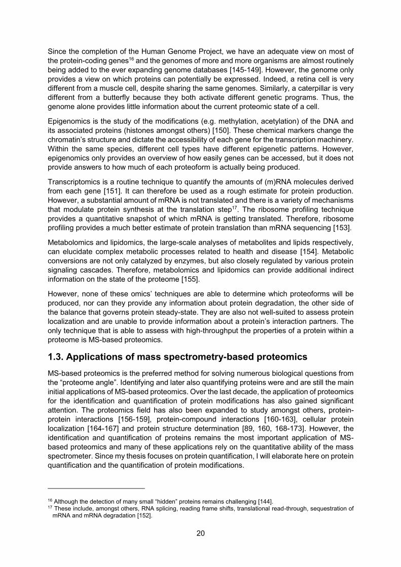
2.1.1. Metabolic labeling ................................................................................................ 24 2.1.2. Post-metabolic labeling ....................................................................................... 26

2.2. Label-free mass spectrometry-based proteomics ...................................................... 29

2.2.1. The label-free proteomics workflow ..................................................................... 29 2.2.2. Advantages and disadvantages of label-free MS-based proteomics .................... 34 2.2.3. Other label-free approaches ................................................................................ 34

xxi

3. From spectra to data ..................................................................................................... 37

3.1. Peptide ion identification ............................................................................................ 37

3.2. Protein inference ........................................................................................................ 40

3.3. Peptide quantification ................................................................................................. 41

3.4. The nature of the data ............................................................................................... 43

3.5. The need for benchmarking ....................................................................................... 46

4. Differential protein abundance analysis ...................................................................... 49

4.1. Preprocessing ............................................................................................................ 49

4.1.1. Transformation .................................................................................................... 49 4.1.2. Filtering ............................................................................................................... 51 4.1.3. Normalization ...................................................................................................... 52 4.1.4. Imputation ........................................................................................................... 55 4.1.5. Summarization .................................................................................................... 57

4.2. Methods for differential protein abundance analysis .................................................. 61

4.2.1. The importance of study design ........................................................................... 61 4.2.2. Summarization-based methods ........................................................................... 63 4.2.3. Peptide-based methods ....................................................................................... 70 4.2.4. Ridge regression ................................................................................................. 73 4.2.5. Robust regression with M estimation ................................................................... 76 4.2.6. Counting-based methods .................................................................................... 79 4.2.7. Controlling the false discovery rate ...................................................................... 81

5. Research hypothesis .................................................................................................... 83

5.1. Setting the stage ........................................................................................................ 83

5.2. Aims of my PhD research ........................................................................................... 85

6. Outline ............................................................................................................................ 87 7. References part I ........................................................................................................... 89


8. Summarization vs Peptide-Based Models in Label-Free Quantitative Proteomics: Performance, Pitfalls, and Data Analysis Guidelines ................................................... 115

8.1. Abstract ................................................................................................................... 115

8.2. Keywords ................................................................................................................. 116

8.3. Introduction .............................................................................................................. 116

8.4. Materials and methods ............................................................................................ 117

xxii

8.4.1. Perseus-based workflows .................................................................................. 118 8.4.2. Summarization-based workflows ....................................................................... 118 8.4.3. Peptide-based models ....................................................................................... 119 8.4.4. Performance ..................................................................................................... 120

8.5. Results ..................................................................................................................... 120

8.6. Discussion .............................................................................................................. 124

8.7. Conclusion ............................................................................................................... 126

8.8. Supporting information ............................................................................................ 127

8.9. Acknowledgement ................................................................................................... 127

8.10. References ............................................................................................................ 127

9. Robust quantification for label-free mass spectrometry-based proteomics .......... 131

9.1. Peptide-level Robust Ridge Regression Improves Estimation, Sensitivity, and Specificity in Data-dependent Quantitative Label-free Shotgun Proteomics .................................... 131

9.1.1. Associated data ................................................................................................ 131 9.1.2. Abstract ............................................................................................................. 132 9.1.3. Introduction ....................................................................................................... 132 9.1.4. Experimental procedures ................................................................................... 136 9.1.5. Results .............................................................................................................. 139 9.1.6. Discussion ......................................................................................................... 146 9.1.7. Footnotes .......................................................................................................... 149 9.1.8. References ........................................................................................................ 149 9.1.9. Appendix ........................................................................................................... 152

9.2. Experimental design and data-analysis in label-free quantitative LC/MS proteomics: A tutorial with MSqRob.................................................................................................... 156

9.2.1. Highlights .......................................................................................................... 156 9.2.2. Abstract ............................................................................................................. 156 9.2.3. Significance ....................................................................................................... 156 9.2.4. Graphical abstract ............................................................................................ 157 9.2.5. Keywords .......................................................................................................... 157 9.2.6. Historical background ....................................................................................... 157 9.2.7. Basic concepts .................................................................................................. 160 9.2.8. How is MSqRob used in research? .................................................................... 163 9.2.9. Case studies ..................................................................................................... 164 9.2.10. Current limitations and useful working limits .................................................... 176 9.2.11. Future developments ....................................................................................... 176 9.2.12. Acknowledgements ......................................................................................... 177 9.2.13. Appendix A ..................................................................................................... 177 9.2.14. References ..................................................................................................... 177 9.2.15. Appendix ......................................................................................................... 185

xxiii

10. MSqRob takes the missing hurdle: uniting intensity- and count-based proteomics .......................................................................................................................................... 187

10.1. Abstract ................................................................................................................. 187

10.2. Introduction ............................................................................................................ 187

10.3. Results and discussion .......................................................................................... 189

10.4. Methods ................................................................................................................ 192

10.4.1. Missing values in recent PRIDE projects ......................................................... 192 10.4.2. Data availability ............................................................................................... 192 10.4.3. Preprocessing for MSqRob and the quasibinomial model ................................ 193 10.4.4. Imputation methods ........................................................................................ 193 10.4.5. Statistical inference ......................................................................................... 194 10.4.6. Code availability .............................................................................................. 197

10.5. Acknowledgements ................................................................................................ 197

10.6. Author contributions ............................................................................................... 197

10.7. References ............................................................................................................ 497

10.8. Appendix ................................................................................................................ 199

PART III: DISCUSSION AND RESEARCH PERSPECTIVES

11. Discussion ................................................................................................................. 203

11.1. Comparing performances ....................................................................................... 203

11.2. The impact of MSqRob .......................................................................................... 206

11.3. The impact of the hurdle model .............................................................................. 209

11.4. Controlling the false discovery rate ........................................................................ 210

11.5. MSqRob compared to other methods ..................................................................... 211

11.6. The impact of technological and algorithmic innovations ........................................ 217

12. Future research perspectives ................................................................................... 221 13. References part III ..................................................................................................... 227

1


3

During the five years of my PhD, I thoroughly investigated different statistical approaches to quantify proteins in label-free mass spectrometry (MS)-based shotgun proteomics. Furthermore, I developed MSqRob, an R package with graphical user interface for the statistically sound analysis of label-free proteomics data. Since I have worked on the interface of protein biology and statistics, it is important to understand both the biological and the statistical aspects of my work.

Hence, in order to place my work in its proper context, this introduction is divided into four chapters. The first chapter aims to give an overview of the biology of proteins and the wide variety of applications of present-day mass spectrometry-based proteomics. In the second chapter, I will describe the technical context of bottom-up quantitative proteomics: the different quantification strategies and the specific peculiarities of the label-free proteomics workflow. In chapter three, I will explain how the spectra are processed into interpretable data. Finally, chapter four will give an overview of how this data can be used to quantify proteins.

5

1. BIOLOGICAL CONTEXT

Chapter 1 mainly aims at introducing proteomics to data analysists who are new to the field. In this chapter, I will first cover the very basics of protein biology (section 1.1). Then, I will give an overview of a generalized mass spectrometry-based proteomics workflow and the relationship of proteomics to other omics (section 1.2), followed by a more profound review of the possibilities of mass spectrometry-based proteomics in present-day life sciences research (section 1.3).

1.1. Proteins as the central effectors of life Before discussing the need for proteomics, I will first introduce the biology of proteins. Proteins are an extremely diverse class of biomolecules that are essential for nearly all functions of life. In this section, I will give an overview of the molecular structure of proteins and how their structures are linked to the essential roles proteins play in health and disease.

1.1.1. The molecular structure and origin of proteins

Proteins are composed of amino acids and the general chemical structure of an amino acid and a protein is given in Fig. 1.1.

Figure 1.1. Chemical structures of a proteinogenic1 amino acid (A) and a protein (B). All amino acids share the same base structure. They all contain an α-amino group (-NH2) and an α-carboxyl group (-COOH) along with a rest group/side-chain (R). The part of the protein ending with the amino group is called the amino- or N-terminus, while the side ending in the carboxyl group is called the carboxyl- or C-terminus. Amino acids differ only in their rest group. In proteins, amino acids are joined together by peptide bonds (-CO-NH-, indicated in red).

1 Proteinogenic amino acids are amino acids that are translationally incorporated into proteins. All proteinogenic

amino acids, except glycine, have an L-stereoisomeric configuration. This means that, when the amino acid is oriented from its N-terminus to its C-terminus as in (A), the rest group (R) will be in front of the plane while the hydrogen atom (H) will be behind the plane. Glycine has no chiral center because its rest group is a hydrogen atom, so the central carbon (α-carbon) is only linked to three different atoms.

6

There are only 20 different standard amino acids2 that can be incorporated in proteins. The actual sequence by which amino acids are joined together is encoded by the corresponding gene found in the genomic DNA (deoxyribonucleic acid). Indeed, in all living organisms, genes are transcribed to RNA (ribonucleic acid) molecules. RNA molecules are composed of only four different nucleotide building blocks holding the nucleobases guanine (G), uracil (U), adenine (A) or cytosine (C). In eukaryotic3 cells, protein-coding RNA, or messenger RNA (mRNA), is then transported from the nucleus (where the grand majority of the DNA resides) to the cytoplasm, where it can be translated into proteins by ribosomes (Fig. 1.2). This unidirectional transfer of information takes place in every living organism: from DNA to mRNA to proteins and has come to be known as the central dogma of molecular biology. Even though some viruses violate this dogma by directly replicating RNA using an RNA template4, or even generate DNA based on an RNA template5, the translation of mRNA to proteins remains a one-way process. RNA is however not always translated into protein. Indeed, RNA itself can have regulatory functions (e.g. micro RNA (miRNA) and long non-coding lncNRA6 can induce gene silencing [7, 8]), structural functions (e.g. ribosomal rNA (rRNA) is an important component of the ribosome [9]) and even catalytic functions (e.g. peptidyl transfer by rRNA, mRNA splicing, self-splicing [10, 11]).

Figure 1.2. The grand majority of transcription occurs in the nucleus of a eukaryotic cell by a protein (or rather, enzyme) called RNA polymerase. Translation occurs in the cytoplasm where ribosomes, specialized cellular structures that are composed of ribosomal RNA and proteins, translate the mRNA into proteins. Both transcription and translation occur from the 5’ to the 3’ end of the oligonucleotides. 5’

2 There are two additional very rare non-standard amino acids that are translationally incorporated into proteins.

Selenocysteine (Sec, U) is present in all domains of life [1], while pyrrolysine (Pyl, O) is only present in 9 methanogenic Archaea of the Methanosarcina family and 15 Bacteria [2]. Both amino acids are present in only a few dozens of proteins.

3 Eukaryotes are cells that, unlike Bacteria and Archaea, have a nucleus. All multicellular organisms (e.g. humans) are eukaryotic, though some eukaryotes are also unicellular.

4 RNA viruses such as rhinoviruses (the most common causes of the common cold) and hepatitis C virus use a protein called RNA-dependent RNA polymerase to make new copies of their RNA genomes.

5 HIV uses the protein reverse transcriptase to convert its RNA genome into DNA and subsequently integrates this DNA into its host’s genome.

6 Note that some short open reading frames in long “non-coding” RNA were shown to generate very small proteins [3-6].

7

and 3’ refer to the conventional chemical names of the carbon atoms in the (deoxy)ribose rings. Proteins are always synthesized from their N- to their C-termini.

Transcription and translation are also unidirectional in space: they always occur from the 5’ to the 3’ terminus of the DNA and mRNA molecules respectively. Each group of three consecutive nucleotides (triplet) in the mRNA represents a codon and each codon represents one unique amino acid or encodes a stop codon. A general overview of the codons that translate into each of the 20 amino acids or are used as stop codons is given in Fig. 1.3. This genetic code is near-universal across the whole tree of life. Some minor exceptions include: yeasts from the CTG clade encode CUG partially or completely as serine instead of leucine [12] and UGA is sometimes translated into tryptophan or arginine instead of being used as a stop codon for some transcripts and some species [13, 14]. Note that all codons, except those for methionine and tryptophan, are redundant: e.g. UUA, UUG, CUU, CUC, CUA and CUG all code for leucine. This property is also called the “degeneracy” of the genetic code.

Figure 1.3. The genetic code. The four mRNA ribonucleosides are guanosine (G), uridine (U), adenosine (A), and cytidine (C). The 20 amino acids are phenylalanine (Phe, F), leucine (Leu, L), isoleucine (Ile, I), methionine (Met, M), valine (Val, V), serine (Ser, S), proline (Pro, P), threonine (Thr, T), alanine (Ala, A), tyrosine (Tyr, Y), histidine (His, H), glutamine (Gln, Q), asparagine (Asn, N), lysine (Lys, K), aspartic acid (Asp, D), glutamic acid (Glu, E), cysteine (Cys, C), tryptophan (Trp, W), arginine (Arg, R) and glycine (Gly, G). Note that each amino acid has both a three-letter abbreviation and a one-letter abbreviation. The AUG codon is the most common start codon and also codes for methionine. Hence, all nascent eukaryotic proteins start with a methionine at their N-terminus when being synthesized7. The three different stop codons (UAA, UAG and UGA) signal translation termination.

However, knowing the mRNA sequence sometimes does not suffice to predict the protein sequence. Indeed, in all domains of life, besides AUG, which is used in more than 80% of the

7 In Bacteria, the start codon codes for N-formylmethionine, but this formyl group is cotranslationally removed [15].

In all domains of life, the N-terminal methionine is often cleaved off, causing more than 50% of the proteins not to have a methionine at the N-terminus [16-18].

8

cases, other codons are also used as start codons [19]. Such so-called near-cognate start codons include CUG, GUG, UUG, ACG, AUC, AUU, AAG, AUA and AGG [20]. In the bacterium Escherichia coli for example, up to 40 out of the 64 codons can be used as start codons, albeit in less than 0.1% of the cases [21]. Such alternative start codons also encode for methionine or N-formylmethionine (in the case of bacteria). If translation is initiated from a downstream8 (near-cognate or canonical) start codon, a shorter protein is produced from the same mRNA template. Similarly, when translation is initiated from an upstream start codon, a longer protein is produced. More rarely, a stop codon can be replaced with another amino acid in a process called translational read-through [22].

Further, in both prokaryotes and eukaryotes, certain “slippery” mRNA sequences, such as AAAAAA, might, under certain circumstances, cause a frameshift, which means that translation continues in another reading frame [23] (Fig. 1.4).

Figure 1.4. Example of a translational frameshift in the dnaX gene of the bacterium Escherichia coli. The dnaX gene encodes both the τ and the γ subunit of the DNA polymerase III protein. dnaX contains a slippery AAAAAA sequence (blue, italics). When the ribosome passes normally over this sequence (top), translation remains in frame and the τ subunit is produced. However, when the ribosome “slips” (bottom), a -1 frameshift occurs. Hereby, a premature stop codon (red, bold) is introduced resulting in the production of the shorter γ subunit. In the dnaX example, ribosome slipping is stimulated by the presence of a downstream stem loop structure in the mRNA that stalls the ribosome. An upstream Shine-Dalgarno like sequence helps repositioning the ribosome in its new reading frame. Example adapted from Dinman (2006) [24].

This ribosomal frameshift is rather rare in most organisms, but very common amongst viruses as it allows them to translate many proteins from a small genome that is limited by the size of the viral particles [24]. Similarly, slippage can already occur at the level of transcription, when the RNA polymerase introduces a variable number of nucleotides in long homopolymeric stretches [25]. Further, it is now also known that amino acids in bacterial proteins can be converted into their D-stereoisomeric form and recent work demonstrates that even a protein’s backbone can be changed by introducing an α-keto-β-amino acid [26, 27].

Besides these rather infrequent phenomena discussed above, alternative RNA splicing is very common as more than 95% of all mammalian genes express alternatively spliced transcripts [28]. Splicing involves the removal of certain parts of an RNA molecule and, dependent on which parts are being spliced out from an mRNA molecule, different protein products can be

8 Downstream means “in the 3’ direction”, upstream is “in the 5’ direction”.

9

generated. Similarly, certain protein sequences, called inteins, are able to post-translationally cut themselves out of a protein [29]. Moreover, proteins are known to carry, often transiently, a plethora of modifications (see also 1.1.3).

Because of these phenomena, many chemically different protein molecules can result from a single gene hence, the term “proteoform” was coined. Proteoforms are defined as “Highly related protein molecules arising from all combinatorial sources of variation giving rise to products arising from a single gene. These include products differing due to genetic variations, alternatively spliced RNA transcripts, and post-translational modifications” [30].

The side-chain of an amino acid determines its physicochemical properties. The nature of a protein will thus not only be determined by the amino acids it contains, but also by the sequence in which they are connected to each other. The specific chemical structures for selected amino acids are given in Fig. 1.5.

Figure 1.5. Examples of the diversity in chemical structures of amino acids: the structures of 6 different amino acids are given. The side-chains of lysine and arginine are long aliphatic chains that are positively charged at physiological pH9. Aspartic acid has a net negative charge at this pH. Tyrosine is a very bulky amino acid that is rather hydrophobic due to the benzene ring in its structure. It is however rather polar due to its hydroxyl (-OH) group. Glycine is the smallest amino acid and the only one that lacks a chiral center as its side-chain itself is a hydrogen atom.

1.1.2. Protein folding

Proteins arrange themselves into three dimensional structures. They are rather flexible, and it is mainly their sequence of amino acids that determines their final 3D structure. The complex interplay of the different chemical properties of the different amino acids will determine a protein’s thermodynamically most favorable 3D conformation. Known physicochemical forces that play a role in protein folding include the hydrophobic effect10, H-bridges, n→π*

9 The average pH inside a cell, which is approximately 7.4 and thus close to the neutral pH 7. 10 Since water is a polar solvent, apolar molecules do not mix well with water. Hence, apolar amino acid residues

will often be found on the inside of a folded protein chain, away from the water that surrounds it. This property is called hydrophobicity (“being afraid of water”).

10

interactions, van der Waals forces, formation of disulfide bridges, the gain of conformational entropy of water on protein folding and electrostatic interactions [31]. Hydrophilic, polar amino acids will mainly be found on the surface of a folded protein, while hydrophobic, apolar amino acids will typically be present on the inside. So-called chaperones are proteins that often aid nascent proteins during the folding process11 to avoid aberrant folding [33]. Sometimes, multiple proteins cluster together to form a functional protein complex (Fig. 1.6).

Figure 1.6. Three-dimensional structure of the protein hemoglobin. Hemoglobin consists of four folded proteins (two α subunits, red, and two β subunits, blue) that are held together by hydrogen bonds. Each subunit is folded such that it creates a pocket that strongly binds an iron-containing heme group (green). Image by Richard Wheeler (Zephyris) at the English language Wikipedia, CC BY-SA 3.0, https://commons.wikimedia.org/w/index.php?curid=2300973.

1.1.3. The JAK-STAT pathway as an example of a protein network

Cells are highly dynamic and thousands of biochemical processes are continuously going on in each cell. Proteins play a crucial role in nearly every one of these processes. The enormous diversity in 3D structures that are adopted by different proteins allows them to bind to other biomolecules with very high specificity. This in turn leads to an immense variety in protein functions. Well-known functions of proteins include, but are definitely not limited to, enzymatic reactions (e.g. trypsin, which digests other proteins in the stomach; kinases, proteins which add a phosphate group to protein substrates), DNA synthesis (DNA polymerases), DNA transcription (RNA polymerases, aided by different sorts of transcription factors), cellular structure (e.g. microtubules), muscle contraction (e.g. actin, myosin) and oxygen transport (hemoglobin).

Therefore, proteins interact both with each other and with other biomolecules. Indeed, most changes inside the cell are triggered by cascades of both stable and transient protein-protein interactions, termed signaling pathways. The JAK-STAT pathway is just one of many intracellular pathways and constitutes a classic example of how a cell responds to a stimulus coming from its environment (Fig. 1.7). JAK-STAT signaling actually is a simple signaling

11 Note that some chaperones also work after translation. Some chaperones aid in stabilizing protein structures in

response to a cellular stressor, others aid in protein unfolding or revert protein aggregation [32].

https://commons.wikimedia.org/w/index.php?curid=2300973

11

cascade and, in reality, such cascades are highly branched, as most proteins have multiple interaction partners.

Figure 1.7. Simplified view of the JAK-STAT pathway. Certain events in the human body can trigger the release of small proteins, called cytokines, in the blood. Some cells are programmed to respond to these cytokines and are therefore equipped with specific cytokine receptors. After binding to an extracellular cytokine, the cytokine receptors dimerize, bringing the JAK kinases in close proximity of each other. The JAKs will subsequently phosphorylate each other on a Tyr residue. The phosphorylated JAKs will then phosphorylate a Tyr residue on the cytoplasmic side of the cytokine receptors. This allows docking of STAT proteins. These STAT proteins will also be phosphorylated by the JAKs. Phosphorylated STATs will dimerize and translocate to the nucleus, where they allow transcription of mRNA molecules encoding for proteins that are needed for the response to the stimulus. Modified after Peter Znamenkiy [Public domain], from Wikimedia Commons.

The JAK-STAT example involves phosphorylation as an illustration of a chemical group that is transferred by a protein (a kinase such as JAK) to another protein (a substrate, here the cytokine receptor, STAT, or JAK itself). In this example, phosphorylation on tyrosines occurs, though it can also occur on serine and threonine residues (as both contain a free hydroxyl (-OH) group) and on the nitrogen atoms of the imidazole ring in histidine residues [34, 35]. Phosphorylation on arginine, lysine, aspartate and glutamate are also known to occur, but are very labile in an acid environment and were therefore proven difficult to study by means of mass spectrometry [36, 37]. Recent work published on BioRxiv proposes a workflow at near-physiological pH that allows the identification of thousands of such non-canonical phosphorylation sites [38]. Moreover, next to phosphorylation, many more co- and post-translational modifications exist, and it is not uncommon for proteins to carry modifications across different residues. These modifications are not only important in signaling cascades, but can also affect protein stability and degradation, alter enzymatic activity and target proteins to membranes [39]. Many diseases (e.g. infectious diseases, auto-immune diseases, neurodegenerative diseases, …) have been linked to aberrant protein modification states [40-43]. A comprehensive overview of all possible protein modifications can be found in the UniMod database at: http://www.unimod.org/modifications_list.php [44].

1.1.4. Proteins in diseases

The extremely complex web of interactions of proteins with each other and with other biomolecules makes that disruption of a single protein’s function often has severe outcomes [45]. Genetic diseases are often the result of a loss-of-function caused by the production of truncated or abnormally folded proteins. For instance, thalassemias are a family of genetic diseases in which an abnormal form of hemoglobin is produced that is less efficient in taking

http://www.unimod.org/modifications_list.php

12

up oxygen [46]. These diseases are caused by one or more mutations in the coding genes that lead to changes in hemoglobin’s amino acid sequence. Such changes can cause substitutions of one amino acid by another but can also result in shorter or longer proteins when stop codons are respectively introduced or erased. They might also impact on mRNA splicing. Large gene deletions or insertions and even fusions with other genes have been reported to cause thalassemia [47]. Such mutations inhibit the production of one or more hemoglobin chains or result in the production of abnormally folded hemoglobin. Mutations can also cause diseases by interfering with the normal modification status of a protein. For example, the severe but rare disease mandibuloacral dysplasia is caused by a single mutation in the gene encoding for the protease ZMPSTE24, which results in the accumulation of toxic farnesylated prelamin A (Fig. 1.8).

Figure 1.8. Left: overview of the maturation of the protein lamin A in healthy individuals. Normally, a hydrophobic farnesyl group is added to lamin A during its preprocessing. Lamin A’s C-terminal end containing the modification is then cleaved off by the ZMPSTE24 protease (here shown as a pair of scissors). Right: in mandibuloacral dysplasia a homozygous mutation12 in the ZMPSTE24 gene causes loss-of-function, which results in the accumulation of toxic farnesylated prelamin A.

Conversely, for many diseases, genetics alone cannot fully explain disease onset. Late-onset Alzheimer’s disease, for instance, has no single genetic cause13. At the protein level, it is characterized by the aggregation of the amyloid-β protein in the brain. Other incurable brain diseases, like Creutzfeldt-Jakob, are caused by a prion, an incorrectly folded protein that causes other proteins of the same kind to take over its aberrant shape, leading to some sort of a chain reaction and massive accumulation of misfolded proteins [50].

12 Humans, like all mammals, have two copies of most genes [48]. ZMPSTE24 loss-of-function only occurs when

both copies are affected. 13 Many different genes influence susceptibility, and the overall genetic heritability is estimated between 60 and

80% [49].

13

1.1.5. Applications of protein research

Proteins are so abundantly being applied throughout our daily lives, that it is nearly impossible to give a complete overview of all their applications. Moreover, researchers continuously strive to improve and broaden protein applications.

In the medical field, proteins are used for diagnosis and disease monitoring. Examples of such biomarkers in blood and plasma approved by the US Federal Drug Administration (FDA) include HE4 for ovarian cancer, CA19-9 for pancreatic cancer and thyroglobulin for thyroid cancer, amongst many others [51], and researchers keep on developing novel biomarker assays.

Determining the 3D structure of proteins is pivotal to their characterization. Indeed, not only do these models allow the prediction of a protein’s interactions with other proteins [52], they also aid in drug development. Nowadays, companies rationally design potential drug candidates by fitting them e.g. onto a protein’s docking site [53, 54]. However, determining a protein’s structure is a non-trivial task. Indeed, although the sequence of a protein will in the end determine its 3D structure, no algorithm exists that can accurately predict 3D structures solely based on amino acid sequences. X-ray crystallography and nuclear-magnetic resonance (NMR) are the most commonly used techniques to determine protein structures, although cryo-electron microscopy is also becoming a viable option [55]. Alternatively, proteins with more than 30% sequence homology are often assumed to have a similar structure [56]. Indeed, such proteins often show an evolutionary relationship and therefore hold a similar structure and function.

Proteins can also be used as therapeutics, with monoclonal antibodies forming the largest class of therapeutic proteins (48% of all FDA approvals in 2011 – 2016) [57]. Examples include antibodies against IL-5 for the treatment of asthma [58], anti-CD319 against relapsed multiple myeloma [59] and anti-VEGFR2 against gastric cancer [60]. New artificial (“recombinant”) proteins can also be produced by modifying the DNA sequence of existing proteins. Examples include ocriplasmin against vitreomacular adhesion [61], glucarpidase against kidney failure [62] and recombinant von Willebrand factor against von Willebrand disease [63]. Proteins are also extensively used in basic biomedical research. Examples include green fluorescent protein (GFP) and its derivatives to visualize proteins inside a cell [64] and the use of Crispr-Cas9 to examine the function of genes by knocking them out or inducing targeted mutations [65].

However, the study of proteins is not only relevant for human diseases. Enzymes, proteins that catalyze biochemical reactions14, are used in sectors as diverse as the pharmaceutical sector, the food industry, paper production, detergent manufacturing and biofuel production [67]. For the production of pharmaceuticals, enzymes aid in the production of precursors or in chemically modifying the final compounds to increase their stability and/or bioavailability [68]. In the food industry, α-amylase is used to convert starch into sugars [69], pectinase to clarify fruit juices [70] and lactase to produce lactose-free milk [71], amongst many others. In the paper industry, xylanase is used to loosen the structure of cellulose fibers, which improves paper quality [72]. Proteases, amylases and lipases are used in laundry detergents to help break down stains of biological origin [73]. Lipases are used in biofuel production to convert free fatty acids to methyl/ethyl esters [74].

14 This acceleration often goes up to several trillions of orders of magnitude [66], allowing reactions that would

naturally take millions of years to occur almost instantly. Previously mentioned proteins such as JAK and ZMPSTE24 are also enzymes: JAK catalyzes a phosphorylation reaction, ZMPSTE24 cleaves a peptide bond.

14

Finally, proteins are also extensively investigated in food crop research. The most well-known example is research on transgenic plants. Here, a DNA sequence coding for a protein with favorable properties is introduced into a commercial crop. This protein can for example promote crop yield or convey resistance against insects, pathogens or herbicides. A notorious example is the development of “golden rice”, a genetically engineered rice variant developed to combat vitamin A deficiency [75]. Indeed, per gram dry weight, the seeds of golden rice contain up to 37 μg β-carotene, a compound that is converted into vitamin A by the human body [76]. Although the rice genome can produce all enzymes needed for β-carotene production, four of these enzymes are not expressed in rice seeds. In golden rice, only two genes are introduced: the psy gene from maize, to produce the enzyme phytoene synthase and the crtI gene from the bacterium Erwinia uredovora to produce the enzyme carotene desaturase. Together, these enzymes restore the β-carotene pathway in the seeds, which results in a rice plant with the typical yellow seeds. Thanks to this simple genetic modification, golden rice holds the promise to save a substantial fraction of the 250,000 to 500,000 children that become blind every year due to vitamin A deficiency, half of which die within a year [77-80]. This is especially the case in Asian countries, where rice is a dominant portion of the standard diet.

Understanding how proteins interact with each other increases our understanding of a plant’s developmental pathways, which allows the breeding of high-yield variants as well as variants that produce stable yields under stress [81]. Indeed, various biotic and abiotic stresses can delay or even terminate plant growth, and even a relatively small, transient stress can markedly reduce crop yield [82]. Hence, researchers actively investigate protein networks involved in stress responses to explain why certain varieties are less stress-sensitive [83, 84]. This knowledge can then later be used for crop improvement through cross-breeding or genetic modification. The lab of my co-promoter is, amongst others, involved in research into protein signaling pathways during the germination of parasitic plants. This is expected to spur the development of germination inhibitors for these plagues [85].

1.2. The nature of mass spectrometry-based proteomics Researchers need to obtain information about the proteome to understand and act upon all these protein-related processes. Proteomics is the study of the proteome and today, MS-based proteomics is the most important proteomic technology. Here, I start by giving a very brief overview of the general principles of chromatography and MS, followed by a discussion of MS-based proteomics workflows. Then, I will situate the proteomics field with respect to the other omics fields.

1.2.1. General principles of liquid chromatography and mass spectrometry

Like every other analytical technique, mass spectrometry has its limitations on the complexity it can efficiently cope with, both in terms of the number of distinct analytes and in terms of differences in the concentrations between these analytes. Separating analytes prior to further analysis is thus essential for reaching sufficient analytical depth. For MS-driven proteomics, the analytes – which are mainly peptides – are present in solution. Hence, liquid chromatography is the method-of-choice for separating peptides prior to analysis by means of mass spectrometry. In liquid chromatographic applications for proteomics, the peptides are first loaded onto a column (also called the stationary phase) in a buffered solution (also called the mobile phase). The composition of the column is such that most (if not all) of the peptides interact with and are thus withheld by this column. By now changing the composition of this mobile phase, the column-bound peptides will start to partition in the mobile phase and are thus eluted from the column at a given composition of this mobile phase. Liquid

15

chromatography can be used to separate peptides based on different physical characteristics such as size, charge and hydrophobicity. Separating peptides based on differences in hydrophobicity is the preferred chromatographic method that is linked to mass spectrometers. In the overall majority of applications, a hydrophobic stationary phase (e.g., chromatographic beads functionalized with C18-groups) is used to bind peptides via hydrophobic interactions. Here, the buffer used to load the peptides is an aqueous buffer. By now gradually increasing the concentration of a water-miscible organic solvent, peptides will start to favor being present in the increasingly organic mobile phase and elute from the stationary phase.

To further analyze the eluted peptides, these peptides need first to be brought into the gas phase and need to get ionized. This process happens in the ionization part of a mass spectrometer. “Soft” ionization techniques, i.e. ionization techniques that transfer little residual energy onto the ions and therefore cause only minimal ion fragmentation have been extremely important for the measurement of intact ions. Indeed, John B. Fenn and Koichi Tanaka were awarded the 2002 Nobel Prize in Chemistry for the development of electrospray ionization (ESI) and soft laser desorption (SLD), respectively. Next to an ionization part, a mass spectrometer also consists of at least one analyzer and at least one detector.

Different types of analyzers have been developed to separate and detect ions based on their mass-to-charge (m/z) ratio. In a time-of-flight (TOF) mass spectrometer, ions are accelerated by a fixed electric field into a vacuum tube. The time it takes for an ion to travel (or fly) through this tube and reach a detector depends on its mass and its charge. Indeed, given the formula of kinetic energy, the higher the mass of an ion, the lower its velocity and thus the later this ion will hit the detector. Conversely, the higher the charge of an ion, the higher its velocity and thus the faster it will hit the detector. The intensity of the signal recorded by this detector is used as a proxy for the initial abundance of the recorded peptide. These signals are recorded at discrete m/z-values at GHz resolution.

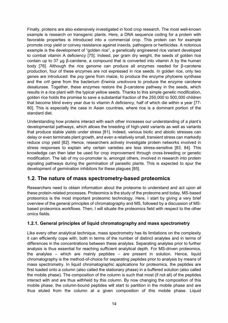
A quadrupole mass analyzer is an example of a more complex analyzer that works as an m/z filter. Quadrupoles consist of four rods, which have an alternating radio frequency voltage with an offset direct current. The frequency voltage and the offset can be tuned in such a way that only ions with a specific m/z value follow a stable trajectory throughout the quadrupole, while all other ions are pushed out (Fig. 1.9). When the quadrupole is used to scan a beam of ions over a certain m/z range, a mass spectrum is recorded.

Figure 1.9. Working principle of a quadrupole. The rods have an alternating radio frequency voltage with a direct current offset. Due to inertia, ions with very high m/z values will be relatively unaffected by the alternating current but will be pushed out of the quadrupole by the non-zero direct current offset. Contrary, ions with very low m/z values will be pushed out of the quadrupole as they are strongly affected

16

by the alternating current. By carefully tuning the alternating and direct currents, a quadrupole works as a very specific ion filter. Figure based on Vékey et al. (2008) [86].

1.2.2. The MS-based proteomics workflow

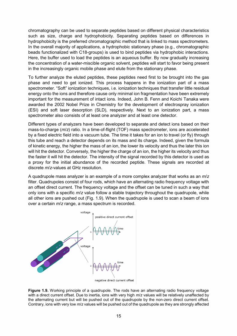
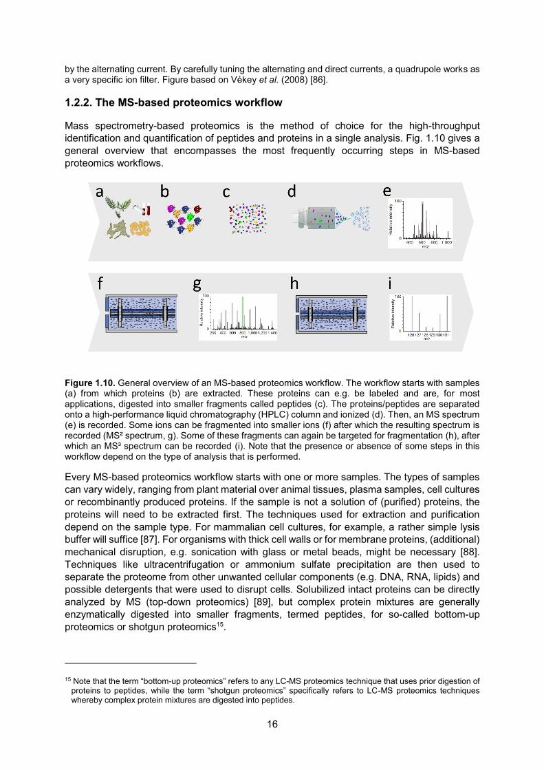
Mass spectrometry-based proteomics is the method of choice for the high-throughput identification and quantification of peptides and proteins in a single analysis. Fig. 1.10 gives a general overview that encompasses the most frequently occurring steps in MS-based proteomics workflows.

Figure 1.10. General overview of an MS-based proteomics workflow. The workflow starts with samples (a) from which proteins (b) are extracted. These proteins can e.g. be labeled and are, for most applications, digested into smaller fragments called peptides (c). The proteins/peptides are separated onto a high-performance liquid chromatography (HPLC) column and ionized (d). Then, an MS spectrum (e) is recorded. Some ions can be fragmented into smaller ions (f) after which the resulting spectrum is recorded (MS² spectrum, g). Some of these fragments can again be targeted for fragmentation (h), after which an MS³ spectrum can be recorded (i). Note that the presence or absence of some steps in this workflow depend on the type of analysis that is performed.

Every MS-based proteomics workflow starts with one or more samples. The types of samples can vary widely, ranging from plant material over animal tissues, plasma samples, cell cultures or recombinantly produced proteins. If the sample is not a solution of (purified) proteins, the proteins will need to be extracted first. The techniques used for extraction and purification depend on the sample type. For mammalian cell cultures, for example, a rather simple lysis buffer will suffice [87]. For organisms with thick cell walls or for membrane proteins, (additional) mechanical disruption, e.g. sonication with glass or metal beads, might be necessary [88]. Techniques like ultracentrifugation or ammonium sulfate precipitation are then used to separate the proteome from other unwanted cellular components (e.g. DNA, RNA, lipids) and possible detergents that were used to disrupt cells. Solubilized intact proteins can be directly analyzed by MS (top-down proteomics) [89], but complex protein mixtures are generally enzymatically digested into smaller fragments, termed peptides, for so-called bottom-up proteomics or shotgun proteomics15.

15 Note that the term “bottom-up proteomics” refers to any LC-MS proteomics technique that uses prior digestion of

proteins to peptides, while the term “shotgun proteomics” specifically refers to LC-MS proteomics techniques whereby complex protein mixtures are digested into peptides.

17

Peptides have the advantage that they are more chemically tractable, more easily separated by liquid chromatography and more easily ionized and fragmented as compared to intact proteins [90-92]. To limit the number of possible peptides in bottom-up proteomics to a reasonable computational search space, the commonly-used protease is highly specific. Trypsin, for instance, is ideally suited, as it cleaves with high specificity after lysine and arginine residues.

Alternative enzymes (e.g. pepsin, chymotrypsin, and the endoproteinases LysC, LysN, AspN, GluC and ArgC) have also been used, as they generate different sets of peptides and therefore reveal complementary parts of a proteome’s sequence space [93-99]. Parallel digestion of the same proteome with multiple proteases can also give a strong boost to the coverage of modification sites [100, 101]. Alternative proteases with more infrequent cleavage specificities will generate longer peptides that can be studied with middle-down proteomics [92, 102, 103]. Nonetheless, trypsin remains the dominant digestion enzyme in bottom-up proteomics. On November 2014, more than 96% of all raw files deposited in the PRIDE repository were using trypsin [102] and there is little reason to assume this percentage has drastically changed today.

To facilitate proteolytic digestion, proteins are often first denatured with urea, which disrupts a protein’s hydrogen bonds causing the protein to denature and unfold. This results in a destruction of protein-protein interactions and a solubilization of hydrophobic lipid-bilayer bound proteins. Urea has the advantage that it can easily be removed by reverse-phase chromatography [104]. However, adding too much urea might also partially denature the protease and hence reduce the digestion efficiency. Further, at higher temperatures, urea partially decomposes into isocyanic acid which carbamylates primary amine groups and thus introduces artefactual amino acid modifications that also block enzymatic digestion [105, 106]. Note that detergents such as sodium dodecyl sulphate (SDS) that are commonly used to lyse cells or to denature proteins prior to polyacrylamide gel electrophoresis (SDS-PAGE), should generally be avoided as they are incompatible with liquid chromatography (LC)-MS [91]. Indeed, even though small amounts of SDS facilitate enzymatic digestion, this detergent suppresses ion signals even at very low concentrations (< 0.01%). SDS cannot be removed with a reverse-phase high-performance liquid chromatography (HPLC) separation step [106-109], although the recently-introduced suspension trapping filter S-TrapTM includes a washing step that makes it compatible with SDS denaturation [110]. Nevertheless, most digestion protocols omit the use of denaturants [111]. Other contaminants may also adversely affect the analysis [112]. It is therefore strongly advised to discuss all preprocessing protocols with proteomics specialists prior to the experiment.

If one is interested in only a subpart of the proteome, additional purification of certain proteins or peptides, e.g. by immunoprecipitation might be needed. Similarly, many protein modifications are transient, have low occupancies, are chemically unstable during standard sample preparation procedures and/or decrease a peptide’s ionization efficiency [113-116]. Therefore, detecting specific modifications requires optimized enrichment protocols [117].

Proteins or peptides are sometimes labeled to facilitate identification and quantification (see section 2.1). These labels can either be small chemical groups or heavy isotopes. They can either be incorporated during the growth of the organism (metabolic labeling, see 2.1.1) or after protein extraction (post-metabolic labeling, see 2.1.2).

Sample pre-fractionation is an option when samples are very complicated and enough protein material is available [118]. Pre-fractionation can be done with a method that is orthogonal to the standard reverse-phase liquid chromatograph that is coupled to the mass spectrometer. Strong cation exchange (SCX) chromatography is a popular pre-fractionation strategy [119]. Although the complexity of each fraction will be reduced, separation is never perfect and many

18

proteins will be present in more than one fraction, which may complicate protein quantification [120]. Each of these samples (or fractions in the case of pre-fractionation) is subsequently analyzed by the mass spectrometer. If the samples are very simple (e.g. a single protein), the proteins/peptides can be directly analyzed by matrix-assisted laser desorption (MALDI) ionization coupled to a time-of-flight mass spectrometer, by which a mass spectrum for the entire sample is obtained [121]. If the samples are more complex, the proteins/peptides are first separated onto a reverse phase liquid chromatography column that is coupled to the mass spectrometer. Upon elution, the proteins/peptides are ionized, typically with electrospray ionization (ESI) [122]. Traditionally, positively charged ions are generated, while neutral molecules and negatively charged ions are filtered out [123]. At discrete time points, the mass spectrometer will measure the mass-to-charge ratios for all the ion species eluting from the column. In the commonly used Orbitrap analyzer, this is achieved by trapping the ions in an orbital motion around a spindle-like electrode, hence the name. The ions are moved back and forth and the fluctuations in charge caused by the movement of the ions are recorded by a detector. This wavelet signal is subsequently converted into a mass spectrum by Fourier transformation. The resulting spectrum is termed an MS or MS1 spectrum. It is important to note that due to the natural occurrence of heavy isotopes of all chemical elements in a fixed ratio, every ion species generates multiple isotopic peaks in the MS spectrum, resulting in a so-called isotopic envelope. Each ion’s charge state is then calculated from the m/z-distance between the peaks in such an isotopic envelope. The summed-up intensities of all ions in an MS spectrum is called the total ion current (TIC). The evolution of the TIC over time is used as a measure of quality control.

In most workflows, an MS spectrum will be insufficient to identify the ion species. Therefore, a single peak in the isotopic envelope of the ions of interest will be selected by the mass spectrometer and targeted for fragmentation. Typically, high intensity peaks are targeted for fragmentation to avoid selecting noise, which would lead to significant losses in operating time. To avoid sequential fragmentations of the same ion during its elution, all previously targeted m/z values are often excluded from being targeted again for a certain amount of time (e.g. 20 seconds). This setting is termed dynamic exclusion and substantially increases the coverage of the mass spectrometer by freeing MS time for the targeting and fragmentation of less intense MS peaks [124].

In shotgun proteomics, collision-induced dissociation (CID) [125] or higher-energy collisional dissociation (HCD) [126] are by far the most common fragmentation methods, while electron-transfer dissociation (ETD) gains popularity for phosphoproteome studies (see 1.3.2) [127, 128]. Negative electron-transfer dissociation (NETD) [123] and photo-dissociation [129-132] are examples of infrequently used fragmentation methods. With CID, ions are collided with noble gasses such as helium and argon that increase the ions’ internal vibrational energy and eventually lead to fragmentation [133]. With HCD fragmentation, the collision energies are higher than 1 keV [134]. Collision therefore occurs in a separate collision cell, typically with a heavier gas, such as dinitrogen [135]. If the peptide’s backbone is fragmented, six types of ions (a, b, c, x, y and z) can be formed, as shown in Fig. 1.11. The mass spectrum of the fragment ions is termed an MS/MS or MS² spectrum.

19

Figure 1.11. Left: overview of the different types of ions that can be formed after fragmentation of a peptide ion’s backbone. a-, b- and c-ions are formed if the charge is retained on the N-terminal peptide fragment. Conversely, x- y- and z- ions are formed if the charge is retained on the C-terminal fragment. Breaking the peptide bond (red) is by far the most energetically favorable fragmentation pattern. Therefore, b- and y-ions will be the most abundant ion species in every MS² spectrum generated by CID or HCD. n is the total number of amino acids in the protein. Modified after Steen and Mann (2004) [136]. Right: example fragmentation pattern for the peptide LDGER. b-ions are indicated in purple, y-ions are indicated in blue. Fragments LDG and ER have the same average mass and therefore form a single peak in the MS² spectrum.

With CID and HCD, b- and y-ions will be far more intense than the other types of ions (a-, c-, x- and z-ions) [137]. For tryptic peptides, CID fragmentation generates both b- and y-ions, while y-ions are much more prominent with HCD fragmentation [137-139].

When the intensities of certain fragment ions are to be used for quantification, MS² fragment ions can optionally be isolated and subjected to mass spectrometry (MS³ spectrum) to prevent interference of other fragment ions with the intensity of the fragment ion of interest. Such MS³ workflows are mainly useful for isobaric labeling (see 2.1.2). Identification of an ion species is typically achieved by searching the fragment ion spectra against a database (see section 3.1).

Note that MS instrumentation is evolving extremely rapidly. Only a few years ago, 20 MS² spectra per second was considered state-of-the-art [140], but the most recent machines now exceed a scanning speed of over 40 spectra per second [141]. This implies that if one MS spectrum is recorded per second, more than 40 peaks in this MS spectrum can be fragmented and thus potentially identified.

1.2.3. Proteomics in relation to other omics

Many omics techniques can provide some information about the state of the proteome, but proteomics is the most suited for this purpose. The fields of genomics, epigenomics, transcriptomics and ribosome profiling largely rely on the analysis of DNA and RNA molecules. RNA can easily be reverse transcribed to DNA and even a single molecule can be readily amplified to billions of copies with a routine polymerase chain reaction (PCR). Moreover, advanced techniques have been devised to sequence and characterize even single RNA and DNA molecules. These possibilities are currently lacking for other types of biomolecules, including proteins. Present-day proteomics relies heavily on mass spectrometry and with the ever-increasing resolutions and operating speeds of contemporary mass spectrometers, the proteomics field has evolved rapidly over the past few years [142, 143]. Other mass spectrometry-based omics fields, such as lipidomics and glycomics, are considered to be still in their infancies.

20

Since the completion of the Human Genome Project, we have an adequate view on most of the protein-coding genes16 and the genomes of more and more organisms are almost routinely being added to the ever expanding genome databases [145-149]. However, the genome only provides a view on which proteins can potentially be expressed. Indeed, a retina cell is very different from a muscle cell, despite sharing the same genomes. Similarly, a caterpillar is very different from a butterfly because they both activate different genetic programs. Thus, the genome alone provides little information about the current proteomic state of a cell.

Epigenomics is the study of the modifications (e.g. methylation, acetylation) of the DNA and its associated proteins (histones amongst others) [150]. These chemical markers change the chromatin’s structure and dictate the accessibility of each gene for the transcription machinery. Within the same species, different cell types have different epigenetic patterns. However, epigenomics only provides an overview of how easily genes can be accessed, but it does not provide answers to how much of each proteoform is actually being produced.

Transcriptomics is a routine technique to quantify the amounts of (m)RNA molecules derived from each gene [151]. It can therefore be used as a rough estimate for protein production. However, a substantial amount of mRNA is not translated and there is a variety of mechanisms that modulate protein synthesis at the translation step17. The ribosome profiling technique provides a quantitative snapshot of which mRNA is getting translated. Therefore, ribosome profiling provides a much better estimate of protein translation than mRNA sequencing [153].

Metabolomics and lipidomics, the large-scale analyses of metabolites and lipids respectively, can elucidate complex metabolic processes related to health and disease [154]. Metabolic conversions are not only catalyzed by enzymes, but also closely regulated by various protein signaling cascades. Therefore, metabolomics and lipidomics can provide additional indirect information on the state of the proteome [155].

However, none of these omics’ techniques are able to determine which proteoforms will be produced, nor can they provide any information about protein degradation, the other side of the balance that governs protein steady-state. They are also not well-suited to assess protein localization and are unable to provide information about a protein’s interaction partners. The only technique that is able to assess with high-throughput the properties of a protein within a proteome is MS-based proteomics.

1.3. Applications of mass spectrometry-based proteomics MS-based proteomics is the preferred method for solving numerous biological questions from the “proteome angle”. Identifying and later also quantifying proteins were and are still the main initial applications of MS-based proteomics. Over the last decade, the application of proteomics for the identification and quantification of protein modifications has also gained significant attention. The proteomics field has also been expanded to study amongst others, protein-protein interactions [156-159], protein-compound interactions [160-163], cellular protein localization [164-167] and protein structure determination [89, 160, 168-173]. However, the identification and quantification of proteins remains the most important application of MS-based proteomics and many of these applications rely on the quantitative ability of the mass spectrometer. Since my thesis focuses on protein quantification, I will elaborate here on protein quantification and the quantification of protein modifications.

16 Although the detection of many small “hidden” proteins remains challenging [144]. 17 These include, amongst others, RNA splicing, reading frame shifts, translational read-through, sequestration of

mRNA and mRNA degradation [152].

21

1.3.1. The analysis of protein and peptide abundance

After a peptide or protein is identified, quantification is the next logical step. Typically, peptides from different biological conditions are labeled either isotopically or chemically in order to induce a mass shift in the MS, MS² or MS³ spectrum. Alternatively, if labeling is omitted (label-free proteomics), mass spectra from different runs should be compared. The peak intensities are a proxy for peptide (and hence a protein) abundance. The peak intensities registered during the elution of a peptide therefore allow for protein quantification in each biological condition. Alternatively, quantification can be done by the less accurate, but simpler spectral or peptide counting. Relating intensities to protein concentrations is challenging because peptides can have very different ionization efficiencies, which are difficult to predict. Nonetheless, there were some attempts at absolute protein quantification [174, 175]. Since the analysis of protein abundance is the focus of my work, I have kept this section intentionally brief since more details about quantitative proteomics are given in chapters 2-4.

1.3.2. The analysis of protein modifications

Both bottom-up and top-down proteomics can be employed to study protein modifications as these cause shifts in the masses of affected peptides that can readily be detected.

As mentioned earlier under 1.1.3, proteins can carry a plethora of modifications. Most of these modifications occur too infrequently to be detected or prove to be very chemically labile. Other modifications, such as the frequently occurring, but often labile phosphorylation, are also difficult to detect because of the poor ionization of the phosphoryl group, which carries a negative charge. Therefore, when the main research goal is to study a certain protein modification, specific enrichment procedures are often required [117].

Phosphorylation is both the most common and the most intensively studied protein modification [176]. Indeed, phosphorylation is a key modification in many signaling cascades and phosphoproteomics has contributed enormously to our understanding of these pathways [177-179]. However, the negative charge of the phosphoryl group and the default usage of positive electrospray ionization makes it difficult to generate and therefore detect positively-charged phosphorpeptides. Thus, phosphopeptides are enriched via pre-fractionation with hydrophilic interaction liquid chromatography (HILIC), Strong cation exchange (SCX) chromatography or strong anion exchange (SAX) chromatography, as well as immunoprecipitation, immobilized metal affinity chromatography (IMAC), metal-oxide affinity chromatography (MOAC), Phos-Tag chromatography, polymer-based metal ion affinity capture (PolyMAC), hydroxyapatite chromatography, enrichment by chemical modification, and/or phosphopeptide precipitation [180]. Negative electron-transfer dissociation (NETD) can also increase the MS intensities of phosphopeptides [123].

Acetylation and methylation are modifications that were first discovered on histones, proteins that are associated with the DNA and package it into structural units called nucleosomes [181, 182]. Histone acetylation is generally associated with open chromatin [183], while histone methylation, dependent on the location of the methylation site, can both be associated with open and closed chromatin [184]. Acetylation can occur both on protein N-termini and on lysine residues [183], while methylation can also occur on arginine residues [184].

Acetylation is important for protein localization [185-188], protein folding [189], protein stability [190] and interactions with other proteins [191]. Methylation is a major factor in important cell signaling pathways such as JAK-STAT, MAPK, WNT, Hippo and BMP [192] and overall protein methylation seems to be strongly intertwined with the organism’s metabolic state [193].

22

Again, enrichment procedures by e.g. (immuno)affinity purification or chromatography are preferable when assessing acetylation or methylation on a proteome-wide scale [194-196].

Glycosylation is another very important post-translational protein modification as over 50% of all mammalian proteins are glycosylated [197]18. Glycosylation plays an important role in protein structure and stability [199-201]. The presence of a glycan structure can block other modifications such as phosphorylation [202]. Glycan structures can be sensed by other proteins (leptins) and play an important role in e.g. cancer and immunity [203, 204]. They are also intensively studied in the context of therapeutic proteins, as many of these proteins carry glycan structures [200, 205]. The enormous complexity of many glycan structures has spurred the development of a new field called glyco(proteo)mics [206].

Ubiquitin is a small 8.6 kDa protein that can be covalently linked to lysine residues of other proteins. However, non-canonical ubiquitination can also occur at Ser, Thr and Cys residues and at a protein’s N-terminal amine group [207]. The earliest known function of K48-linked19 polyubiquitination is the degradation of the modified proteins in the proteasome. This discovery resulted in the 2004 Nobel Prize in Chemistry for Avram Hershko, Aaron Ciechanover, and Irwin A. Rose [208]. Although K11-linked polyubiquitination can also result in proteasomal degradation [209], ubiquitin is also an important scaffold that allows recruitment of other proteins and plays an important role in cellular processes as diverse as e.g. protein trafficking, mitophagy and cell cycle control. Next to K48 and K11; K6, K27, K29, K33 and K63 linkages have also been described. Many proteins are mono-ubiquitinated, but ubiquitin chains can also be linear and branched and even combined with other small ubiquitin-like modifiers such as SUMO and NEDD-8 [210].

Detection of ubiquitination by MS is challenging because ubiquitin is often either quickly degraded by the proteasome or part of very dynamic signaling pathways [211]. Moreover, ubiquitin is much bigger than most other small modifications. Being a protein, ubiquitin is also degraded by trypsin, leaving only a small GG or LRGG tag behind [212, 213]. Finally, ubiquitination does not seem to occur on well-defined amino acid sequence motifs [214-216]. Nonetheless, protocols for proteome-wide detection of ubiquitination are now readily available thanks to innovative purification and chemical tagging strategies [211, 217]. Similarly, protocols have also been developed for the proteomic analysis of other less characterized small ubiquitin-like modifiers like SUMO [218, 219], NEDD-8 [220, 221] and ISG [222, 223].

18 Note that not only proteins, but also lipids can be glycosylated [198]. 19 K48-linkage means that each ubiquitin in the chain is linked to the previous ubiquitin via the lysine (K) residue at

position 48 (starting from the N-terminus).

23

2. TECHNICAL CONTEXT

As amply demonstrated in the previous chapter, mass spectrometry-based proteomics has become an invaluable tool for protein researchers. In chapter 2, I will discuss the different flavors of mass spectrometry-based proteomics with a focus on their technicalities. I will specifically emphasize label-free shotgun proteomics, as all my PhD work revolves around this particular technique. This technical overview will provide a handle for chapter 3, where I will link the statistical challenges to the technology.

2.1. Label-based mass spectrometry-based proteomics Traditionally, quantitative proteomics has made use of stable-isotope coded labels. This used to be a necessity, as the peptides that were identified often differed strongly between LC-MS/MS runs. Indeed, even minor differences in electrospray voltages and/or chromatographic flow rates increase the run-to-run variability in signal intensities and hence reduce the precision of label-free quantification [224, 225]. By metabolically labeling proteins from different samples and subsequently pooling these together for a single analysis, it became possible to identify the peptides in each sample analyzed and remove the inter-sample variability. In fact, one distinguishes two categories of label-based proteomics: metabolic and post-metabolic labeling.

In metabolic labeling, labels are incorporated during cell or organism expansion. By contrast, in post-metabolic labeling, a label is added after protein extraction or even after protein digestion, typically by means of a chemical reaction that targets specific reactive groups in proteins or peptides. The main advantage of metabolic labeling is that the labeled proteins can immediately be pooled together, thus any random or systematic experimental errors that occur after pooling will affect all samples equally [226]. Thereby, this unwanted variability can be factored out from the analysis, which increases the overall precision. Post-metabolic labeling, by contrast, does not affect the biology of the organism under study (see below), as labeling only occurs after protein extraction. And, although post-metabolic labeling requires more protein material, it is more broadly applicable [227]. Fig. 2.1 gives an overview of the experimental stages in which labels are introduced and samples are mixed for different labeling protocols.

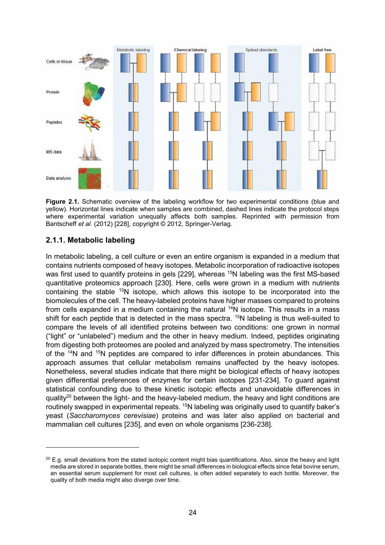
24

Figure 2.1. Schematic overview of the labeling workflow for two experimental conditions (blue and yellow). Horizontal lines indicate when samples are combined, dashed lines indicate the protocol steps where experimental variation unequally affects both samples. Reprinted with permission from Bantscheff et al. (2012) [228], copyright © 2012, Springer-Verlag.

2.1.1. Metabolic labeling

In metabolic labeling, a cell culture or even an entire organism is expanded in a medium that contains nutrients composed of heavy isotopes. Metabolic incorporation of radioactive isotopes was first used to quantify proteins in gels [229], whereas 15N labeling was the first MS-based quantitative proteomics approach [230]. Here, cells were grown in a medium with nutrients containing the stable 15N isotope, which allows this isotope to be incorporated into the biomolecules of the cell. The heavy-labeled proteins have higher masses compared to proteins from cells expanded in a medium containing the natural 14N isotope. This results in a mass shift for each peptide that is detected in the mass spectra. 15N labeling is thus well-suited to compare the levels of all identified proteins between two conditions: one grown in normal (“light” or “unlabeled”) medium and the other in heavy medium. Indeed, peptides originating from digesting both proteomes are pooled and analyzed by mass spectrometry. The intensities of the 14N and 15N peptides are compared to infer differences in protein abundances. This approach assumes that cellular metabolism remains unaffected by the heavy isotopes. Nonetheless, several studies indicate that there might be biological effects of heavy isotopes given differential preferences of enzymes for certain isotopes [231-234]. To guard against statistical confounding due to these kinetic isotopic effects and unavoidable differences in quality20 between the light- and the heavy-labeled medium, the heavy and light conditions are routinely swapped in experimental repeats. 15N labeling was originally used to quantify baker’s yeast (Saccharomyces cerevisiae) proteins and was later also applied on bacterial and mammalian cell cultures [235], and even on whole organisms [236-238].

20 E.g. small deviations from the stated isotopic content might bias quantifications. Also, since the heavy and light

media are stored in separate bottles, there might be small differences in biological effects since fetal bovine serum, an essential serum supplement for most cell cultures, is often added separately to each bottle. Moreover, the quality of both media might also diverge over time.

25

Incomplete labeling is a major disadvantage of all metabolic labeling strategies. Indeed, natural medium still contains a non-negligible albeit very low amount of heavy isotopes (e.g., 1% 13C and 0.4% 15N ) [239]. Similarly, medium highly enriched in heavy isotopes still contains a fraction of lighter isotopes. As peptides differ in their number of amino acids and different amino acids have different numbers of atoms, isotopic labeling will generate a plethora of different partially unlabeled variants for every peptide analyzed [240]. Therefore, the mass shift of a peptide after labeling depends on its composition, which complicates downstream peptide identification and quantification.

Stable Isotope Labeling by Amino acids in Cell culture (SILAC) is a metabolic labeling approach where amino acids, typically essential amino acids, containing one or more stable heavy isotopes are used for differential protein quantification [241, 242]. The use of amino acids as opposed to isotopically labeled nutrients has greatly simplified data analysis for MS-based protein quantification, and this because the labeled amino acids are incorporated into proteins, implying that a peptide’s mass shift can be directly derived from its amino acid composition. An important point is that the organism in the heavy condition needs to be exposed to the heavy-labeled amino acids for long enough to allow the complete replacement of the organism’s natural (unlabeled) amino acids by the supplied heavy amino acids. For cell cultures, seven doubling times seems to be sufficient to allow full incorporation, even for proteins with very slow turnover rates [240]. By contrasting light (e.g. 12C6

14N4-arginine), medium (e.g. 13C6

14N4-arginine) and heavy (e.g. 13C615N4-arginine) SILAC labeling, three

different conditions can be directly compared [243]. In 2010, the introduction of 5-plex SILAC allowed the comparison of up to five different conditions in a single MS run [244]. When more than five conditions need to be compared with SILAC, a heavy-labeled standard proteome can be spiked into every condition and be used as a reference to allow calculation of the protein ratios for every comparison (super-SILAC) [245] [246]. SILAC-labeling was initially confined to cell cultures, but over time, it has been expanded to organisms such as the worm Caenorhabditis elegans [247], the fruit fly Drosophila melanogaster [248], mice [249] and plants [250]. Fig. 2.2 gives an overview of a typical SILAC workflow.

Figure 2.2. Overview of a SILAC workflow where three experimental conditions need to be compared. The proteomes from the light, medium-labeled and heavy-labeled conditions can be pooled together and analyzed in a single MS run. The intensity ratios of the triplets for each peptide ion species can then

26

be directly calculated from its corresponding MS spectrum. Reprinted with permission from Geiger et al. (2011) [251], copyright © 2011, Springer-Verlag.

Also, the isotopic purity of the SILAC medium is of utmost importance. When the fraction of “heavy” amino acids is insufficiently high, the hence-labeled proteome contains a substantial fraction of “light” amino acids, leading to quantification biases in the direction of the “light” condition [240]. Further, when using trypsin to digest an arginine-SILAC labeled proteome, a possible caveat is introduced by the metabolic conversion of arginine into proline and glutamate [252], which introduces extra stable isotopes in proline-containing peptides, thereby obstructing accurate quantification. This can be prevented by adding an excess of unlabeled proline [253, 254] and/or by reducing the arginine concentration [255].

SILAC requires dialyzed fetal bovine serum as no other variants of the selected essential amino acids other than the labeled variants must be present in the medium. Dialysis however results in the loss of growth factors, which will cause a cellular stress response that might bias the response to the treatment of interest or even completely prevent cell or organism growth altogether [227, 256].

Despite its main advantage of factoring out run-to-run variability from each comparison, SILAC seems to be slowly getting out of favor for high-throughput protein quantification. The main reason is that the quantification depth (i.e. the number of proteins identified) of SILAC is reported to be ~30 to 60% lower than the quantification depth of label-free quantification (see 2.2.1) [257, 258], although this difference also depends on sample complexity and instrument resolution. Indeed, as multiple SILAC-labeled samples are jointly analyzed in a single MS run, the amount of protein analyzed per experimental condition is two to five (for 5-plex SILAC) times lower, while the number of peaks in each MS spectrum increases with the same factor [258, 259]21. In such complex spectra, the peptide ion signals will be lower and might even become indiscernible from the background noise. Also, the more peaks, the higher the chances of co-fragmentation: i.e. two (or more) peptide ions with overlapping isotopic envelopes are fragmented together, increasing the risk of unidentifiable spectra [260]. Moreover, as all isotopic variants of the same peptide can be targeted for identification, less MS peaks might be identified due to limitations on the MS² sampling rate [261]. Another disadvantage of metabolic labeling is that its dynamic range is generally smaller than those of label-free and isobaric quantification approaches (see 2.1.2 and 2.2.1) [262-265]. Also, isobaric labeling appears to have a higher precision [265].

Recently, neutron-encoded (NeuCode) labeling has been proposed as a promising new metabolic labeling approach that relies on the ability of modern high-resolution MS to distinguish extremely small mass differences (in the orders of mDa) [261, 266]. However, NeuCode did not gain a lot of traction yet because of the extremely high cost of its reagents, which seriously limits its throughput.

2.1.2. Post-metabolic labeling

In post-metabolic labeling, a different chemical label is added to each sample after protein extraction or digestion. Post-metabolic labeling strategies are often used for large experiments in which many samples need to be compared because of their superior opportunities to simultaneously measure multiple experimental conditions in a single MS run (“multiplexing”). In the context of high-throughput protein quantification, labels are added after digestion

21 The reason is that the total amount of peptides (in µg) that is spiked onto the mass spectrometer is a fixed

constraint. Under-spiking will result in low signal intensities and hence low proteome coverage, while over-spiking will result in signal saturation.

27

because this allows labeling of peptides that are buried within a protein’s 3D structure, resulting in a higher peptide coverage.

Dimethylation is one of the oldest post-metabolic labeling strategies, though still widely used as it is easy to multiplex and fairly cheap [267]. Indeed, dimethylation requires relatively cheap reagents such as isotopically labeled formaldehyde and cyanoborohydride [268]. Here, all lysine side chains and peptide N-termini are dimethylated, except if the N-terminus starts with proline, in which case it will be monomethylated [269]. Originally performed in duplex [270], dimethylation was expanded to 3- [271], 4- [272] and 5-plex labeling [273]. By combining dimethylation with SILAC, 6-plex labeling has been achieved [274]. Compared to SILAC, dimethylation has a similar dynamic range and accuracy [265, 275]. Thus, the additional experimental variability introduced by post-metabolic labeling as compared to metabolic labeling seems to be limited in practice. Deuterium was used in the dimethylation approaches described above. However, compared to hydrogen-1, deuterium binds less strongly to the hydrophobic stationary phase due to the lower amplitude of its vibrational frequencies [276]. This results in a chromatographic shift as deuterium-labeled peptides elute somewhat earlier than their hydrogenated counterparts, which increases the uncertainty on the ratios of their peak intensities [277, 278]. Therefore, most contemporary isotopic labeling strategies avoid deuterium and favor e.g. 13C, which does not induce a noticeable chromatographic shift [279]. 18O labeling is an enzymatic post-metabolic labeling approach that was originally used to improve peptide identification [280-282]. Soon after, 18O labeling also became a tool for protein quantification [283-286]. Here, protein digestion is performed either in normal water or in 18O-rich water. Two 18O-atoms are incorporated at the peptides’ C-termini, resulting in 4 Da mass shifts. Nowadays, 18O labeling is not very common anymore as 18O incorporation efficiency is variable and the technique cannot be multiplexed [287].

Isobaric labeling relies on mass differences in the fragment ions of isotopologic tags to quantify peptide ions via their MS² spectra. Indeed, the isobaric labels in each condition have the same total nominal mass, but a specific fragment ion, the reporter ion, has different masses for each label. Differentially labeled peptides thus coincide in the MS spectrum, but the reporter ions allow for quantification in the MS² spectrum. iTRAQ [288] and TMT [227] are the most well-known and frequently used reagents for isobaric labeling (Fig. 2.3).

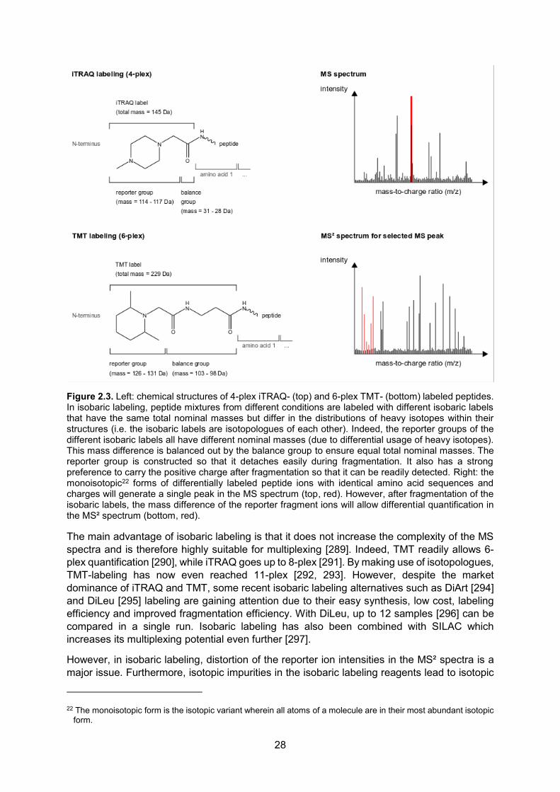
28

Figure 2.3. Left: chemical structures of 4-plex iTRAQ- (top) and 6-plex TMT- (bottom) labeled peptides. In isobaric labeling, peptide mixtures from different conditions are labeled with different isobaric labels that have the same total nominal masses but differ in the distributions of heavy isotopes within their structures (i.e. the isobaric labels are isotopologues of each other). Indeed, the reporter groups of the different isobaric labels all have different nominal masses (due to differential usage of heavy isotopes). This mass difference is balanced out by the balance group to ensure equal total nominal masses. The reporter group is constructed so that it detaches easily during fragmentation. It also has a strong preference to carry the positive charge after fragmentation so that it can be readily detected. Right: the monoisotopic22 forms of differentially labeled peptide ions with identical amino acid sequences and charges will generate a single peak in the MS spectrum (top, red). However, after fragmentation of the isobaric labels, the mass difference of the reporter fragment ions will allow differential quantification in the MS² spectrum (bottom, red).

The main advantage of isobaric labeling is that it does not increase the complexity of the MS spectra and is therefore highly suitable for multiplexing [289]. Indeed, TMT readily allows 6-plex quantification [290], while iTRAQ goes up to 8-plex [291]. By making use of isotopologues, TMT-labeling has now even reached 11-plex [292, 293]. However, despite the market dominance of iTRAQ and TMT, some recent isobaric labeling alternatives such as DiArt [294] and DiLeu [295] labeling are gaining attention due to their easy synthesis, low cost, labeling efficiency and improved fragmentation efficiency. With DiLeu, up to 12 samples [296] can be compared in a single run. Isobaric labeling has also been combined with SILAC which increases its multiplexing potential even further [297].

However, in isobaric labeling, distortion of the reporter ion intensities in the MS² spectra is a major issue. Furthermore, isotopic impurities in the isobaric labeling reagents lead to isotopic

22 The monoisotopic form is the isotopic variant wherein all atoms of a molecule are in their most abundant isotopic

form.

29

overlaps in neighboring reporter ion intensities. Prior to data analysis, each reporter ion peak should therefore be corrected for isotopic overlap using correction factors supplied by the reagent manufacturer [298]. Another issue is that co-eluting near-isobaric peptide ions are isolated and co-fragmented with the target peptide ion, skewing the ratios of the reporter ion intensities towards the median value over all proteins, which is usually very close to one23. For this reason, this phenomenon is also called ratio compression [298-300].

Several technical solutions have been developed to reduce ratio compression. Gas-phase purification [301] and ion mobility separation [302] remove interfering ion species prior to fragmentation. MS³ prevents co-fragmentation by isolating an MS² peptide fragment ion and fragmenting it again to produce an MS³ spectrum. This additional step massively reduces the chance that the selected fragment ion will again be co-isolated with a fragment ion from another peptide species. As this MS² fragment ion contains all the isobaric labels, the reporter ions in the MS³ spectrum enable more accurate and more reproducible protein quantification [303].

Even with these improvements, around 8% of the MS³ spectra remain affected by co-fragmentation [265]. The introduction of synchronous precursor selection MS³ (SPS-MS³), in which multiple MS² fragment ions of a precursor peptide are co-isolated, strongly boosts MS³’s sensitivity [304]. However, despite clear progress, MS³ still requires complex instrumentation and has a slower duty cycle, resulting in a lower identification depth compared to MS² quantification [289]. TMTc and EASI tag are new strategies whereby the complement ions (i.e. peptide fragments that remain attached to the balance group) are quantified in the MS² spectrum [289, 305, 306]. These approaches avoid both the complexities of MS³ and the unwanted ratio compression because they examine the isotopic envelope of a particular labeled MS² peptide ion fragment.

Disadvantages of isobaric labeling include the loss of quantification depth and the poor accuracy for quantifying low-intensity peaks due to the lower signal-to-noise ratio in MS² spectra compared to MS spectra [265, 307]. The former can be partially alleviated by pre-fractionation. However, this results in longer run times and a more complicated data analysis [308, 309]. MS²-based quantification also implies that only those peptides that are selected for fragmentation can be used for quantification [266]. Hence, for the many proteins that are identified with few peptides, it is difficult to assess the precision on their differential abundance estimates. Finally, iTRAQ and TMT labeling are relatively costly [275].

2.2. Label-free mass spectrometry-based proteomics My PhD work is centered around the quantification of data-dependent label-free discovery-based shotgun proteomics data. Therefore, I will here give an extensive overview of the label-free shotgun proteomics workflow.

2.2.1. The label-free proteomics workflow

An overview of a generalized proteomics workflow has already been given in 1.2.2. In this section, I will focus on the aspects that are specific to label-free proteomics, and more specifically on those aspects that pose challenges to the ensuing data analysis.

A label-free proteomic workflow consists of the following steps: (1) proteins are extracted from the sample, (2) these proteins are digested into peptides, (3) the peptides are separated by reverse phase HPLC (RP-HPLC), (4) eluting peptides are ionized, (5) an MS spectrum is taken, (6) a precursor ion is selected, (7) this precursor ion is fragmented and (8) an MS² spectrum 23 The total amounts of peptides loaded and analyzed are usually equal for all samples.

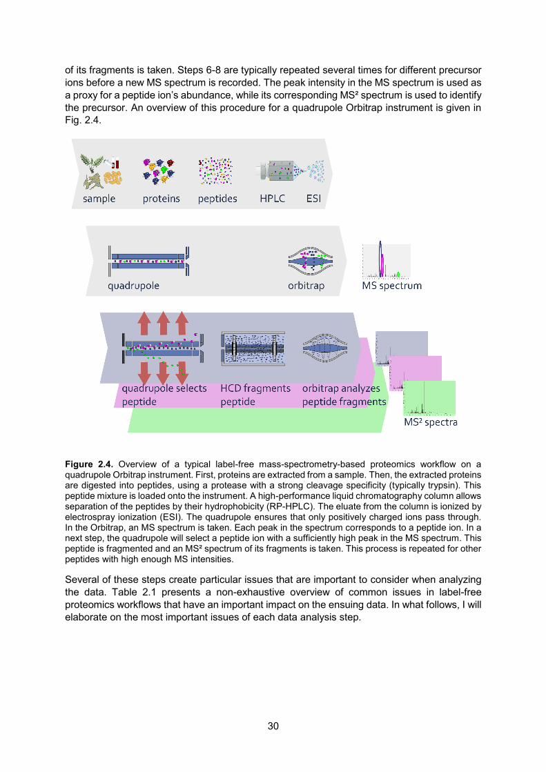
30

of its fragments is taken. Steps 6-8 are typically repeated several times for different precursor ions before a new MS spectrum is recorded. The peak intensity in the MS spectrum is used as a proxy for a peptide ion’s abundance, while its corresponding MS² spectrum is used to identify the precursor. An overview of this procedure for a quadrupole Orbitrap instrument is given in Fig. 2.4.

Figure 2.4. Overview of a typical label-free mass-spectrometry-based proteomics workflow on a quadrupole Orbitrap instrument. First, proteins are extracted from a sample. Then, the extracted proteins are digested into peptides, using a protease with a strong cleavage specificity (typically trypsin). This peptide mixture is loaded onto the instrument. A high-performance liquid chromatography column allows separation of the peptides by their hydrophobicity (RP-HPLC). The eluate from the column is ionized by electrospray ionization (ESI). The quadrupole ensures that only positively charged ions pass through. In the Orbitrap, an MS spectrum is taken. Each peak in the spectrum corresponds to a peptide ion. In a next step, the quadrupole will select a peptide ion with a sufficiently high peak in the MS spectrum. This peptide is fragmented and an MS² spectrum of its fragments is taken. This process is repeated for other peptides with high enough MS intensities.

Several of these steps create particular issues that are important to consider when analyzing the data. Table 2.1 presents a non-exhaustive overview of common issues in label-free proteomics workflows that have an important impact on the ensuing data. In what follows, I will elaborate on the most important issues of each data analysis step.

31

Table 2.1. Non-exhaustive list of issues that arise during a label-free shotgun proteomics workflow and their impact on the data.

Analysis step Issues Consequences Protein extraction Differences in extraction

efficiencies Variable protein concentrations over different samples

Protein digestion Unequal enzymatic cleavage efficiencies, non-canonical cleavage, peptide ragging

Unequal concentrations of peptides originating from the same protein

RP-HPLC separation Technical variability in elution times

Difficulties in matching unidentified peptides to identified peptides across different runs

Peptide carry-over due to peptides from previous runs that did not elute from the column

Detection of peptides that were not present (worst case), peptide intensities influenced (increased) by the order in which the samples were run

ESI ionization Strong differences in peptide ionization efficiencies

Strong differences in MS intensities for peptides originating from the same protein

ESI saturation: peptides compete for ionization

Ionization suppression: a peptide’s MS intensity (partially) depends on the nature and amount of other co-eluting peptides

Suppression of high MS intensities resulting in an upper limit of quantification

Peptides ionize in different charge states

Intensities for different charge states need to be taken into account when quantifying a peptide

Gas-phase peptide ions undergo chemical reactions

Artificial peptide modifications, which are possibly not accounted for, resulting in unidentifiable spectra and missing values

Changes in electrospray voltage during and across different runs

Increased variability in peptide ionization efficiencies

MS recording Discrete MS spectrum recording

MS intensity not recorded at the elution peak

MS detector saturation Suppression of high MS intensities resulting in an upper limit of quantification

MS² recording Limited amount of MS peaks targeted for fragmentation

Different peaks fragmented across different runs: missing values

Preferential targeting of high-intensity MS peaks

Intensity-dependent missing values

Loss of unexpected peptide fragments

Difficulties in MS² spectrum identifications and thus missing values

Co-fragmentation of peptide ions with similar m/z values

Unidentifiable chimeric MS² spectra and thus missing values

32

The first step in the protocol, protein extraction, was shown to be responsible for 72% of all technical variability [310]. However, small differences in protein extraction efficiencies generally should not pose too much problems as an equal amount of total peptides is loaded onto the instrument for every sample. As noted in 1.2.2, it is imperative that all sample preprocessing is compatible with RP-HPLC-MS. It is therefore important to limit or avoid the use of urea [105, 106] and to avoid the use of SDS [91, 106-109] as well as other contaminants [112].

The digestion step is also critical. If the digestion efficiencies differ between samples, certain peptides might be formed to different extents. Consider for example the proteolytic cleavage of the following protein:

SESNAHFSFPKEEEKEFLESYPQNCPPDALPGTPGNLDSAQELEGFQIPTNLDWAGTSQAR

The most commonly used protease, trypsin, cleaves at the C-terminus of lysine (K) and arginine (R) (indicated in red) [311]. Depending on the digestion efficiency, varying amounts of the peptides SESNAHFSFPK and SESNAHFSFPKEEEK can be identified. Both the very short EEEK peptide and the very long EFLESYPQN…R peptide are barely or not detected by the mass spectrometer. Peptide SESNAHFSFPKEEEK is said to have one missed cleavage site, but peptides can have multiple missed cleavages. The presence of missed cleavages not only depends on the duration of the digestion, but also on the quality of the enzyme [312]. However, peptides can also be formed at non-canonical cleavage sites (i.e. not at lysine’s or arginine’s C-terminus) and modifications (either of biological origin or artifacts formed during sample preprocessing) may affect enzymatic digestion efficiency [311]. Next to these elements, the amino acids adjacent to a possible cleavage site, the location of a peptide in a protein’s 3D structure and chemical degradation also play a role in the kinetics of the generation and degradation of different peptide species. Moreover, unwanted chemical reactions during sample preprocessing and/or the activities of exopeptidases that might be present in the sample or as contaminants in the commercial protease batch may cause N-terminal or C-terminal peptide degradation (“peptide ragging”) [313]. For these reasons, the concentrations of most peptides are not equal to the initial protein concentration [314]. This stresses the importance of uniformity in the digestion conditions over the different samples.

Since the RP-HPLC column is typically packaged with porous silica beads coated with apolar alkyl chains (e.g. C18), peptides will be separated by their differences in hydrophobicity [315]. Protein modifications can however influence the column retention of an affected peptide [316]. Further, there is inherent variability in the chromatographic retention of a given peptide over different MS runs. This is an important factor to bear in mind when matching an identified peak in one MS run to an unidentified peak in another run; so-called matching between runs [317]. Comparing retention times over different runs is routinely done by algorithms for retention time alignment [318]. Retention times are often monitored as a general quality control measure by spiking in a known peptide or peptide mix [319, 320] and several algorithms have been developed to predict the retention times of known peptides [315, 321-323]. In order to maximize the mass spectrometer’s operation time, HPLC columns are generally not replaced between analyses. Therefore, peptides from a previous injection might partially remain retained on the column and elute during a subsequent run, thus leading to the detection of peptides that were not present in that last sample and/or biased quantifications. Little has been published in the literature about sample carry-over, even though this is a non-negligible problem [324].

Peptide elution happens continuously, while the mass spectrometer only generates mass spectra at discrete time points. As peptide elution takes around 5 – 25 seconds [325, 326] and modern mass spectrometers typically tend to record an MS spectrum every second, the intensity peak for a single peptide ion will be recorded in sequential MS spectra. To allow for

33

an accurate quantification, it is important to record at least one MS peak at or near each peptide’s elution apex. High-resolution RP-HPLC separation concentrates peptides in narrower elution peaks and is highly beneficial for different reasons [141]. First, repeated fragmentations of the same peptide ion over its elution window are highly reduced, thus winning MS analysis time. Next, highly focused peptide elution increases ion intensities and the ability to target monoisotopic peaks, which facilitates identification. Finally, an improved separation reduces co-elution of peptides, preventing ion suppression and co-fragmentation (see below).

The quality of ionization is of utmost importance as poor ionization leads to lower quality spectra (lower signal-to-noise ratio), making it more difficult to identify and quantify peptides. The electrospray voltage should also be kept as constant as possible over different runs as even small voltage deviations aggravate the variability in ionization efficiencies of peptides over different runs, which reduces the precision of label-free quantification [225].

During electrospray ionization (ESI), peptides are endowed with a positive charge (when working in positive ionization mode) [122]. However, the ionization efficiency of peptides differs. For example, highly acidic peptides and phosphopeptides ionize more poorly [123]. Such different ionization efficiencies leads to different MS intensities across different peptides, even if their concentrations are equal. In addition, the ionization efficiency of a peptide is also influenced by the nature and the amount of co-eluting peptides as these may suppress each other’s ionization, a phenomenon known as ionization competition or ionization suppression [122, 327]. For these reasons, peptide ionization efficiencies are still difficult to predict [328]. Finally, the total amount of peptides that can be ionized simultaneously is also limited due to saturation effects during ionization [329, 330], which results in a suppression of high MS intensities and therefore an upper limit on the amount of peptides that can be quantified.

Ionization also generates different ion species from a single peptide, which differ in charge state. Indeed, ESI typically generates multiple ions with different charge states from the same peptide. For tryptic peptides, a double positive (+2) charge state is the by far most common after ESI ionization (around 75 - 90% of all ions), followed by triple positive (+3, around 10 - 20% of all ions) and single positive (+1, around 5% of all ions) [331]. The ionization step might also affect the chemical composition, and hence the mass, of an ion. Examples include in-source peptide oxidation and the loss of water or ammonia from N-terminal glutamate or glutamine residues, respectively, to form pyroglutamate [332, 333].

In the MS spectrum, the intensity of every ion that eluted from the HPLC column at that particular point in time is recorded in function of its mass-to-charge (m/z) ratio. Ion intensities can be seen as proxies for abundance, with the caveat that the ionization efficiencies differ strongly between different ion species. The detector of the mass spectrometer is also sensitive to saturation, which might also result in suppression of high MS intensities [329, 330].

After the generation of the MS spectrum24, a high-intensity ion species is isolated with the quadrupole and targeted for fragmentation, a process that is repeated several times before a new MS spectrum is recorded. High-intensity MS peaks are intentionally targeted for fragmentation to avoid the targeting of noise peaks and hence increase the depth of the analysis. However, the fact that not all peaks in an MS spectrum can be targeted for fragmentation and the fact that high-intensity peaks are preferentially selected, results in intensity-dependent missing values. Dynamic exclusion, whereby previously-targeted m/z

24 Or sometimes during the generation of the MS spectrum, if the machine has two mass analyzers.

34

values are temporarily excluded from fragmentation increases the quantification depth but does not alleviate the issue of intensity-dependent missingness.

Fragmentation also commonly results in neutral losses of water and ammonia, or even partial or complete amino acid side chains [137]. Such losses need to be taken into account when identifying a peptide ion based on its MS² spectrum. To facilitate identification, it is also preferable that the monoisotopic peak is correctly determined. For short peptides, the monoisotopic peak is often the highest one, but for longer peptides, this peak might be considerably smaller. This sometimes leads to determination of the wrong peak in the isotopic envelope and hence a wrong selection of candidate peptides during database filtering. Finally, when one or more peptides of about the same m/z elute together with a target peptide ion, such neighboring ions can be isolated as well, resulting in a mixed MS² spectrum [334]. Such a mixed fragmentation spectrum will also cause problems regarding identification and quantification.

2.2.2. Advantages and disadvantages of label-free MS-based proteomics

An obvious advantage of label-free MS-based proteomics is that the laborious and often costly labeling is omitted altogether [226]. Moreover, label-free analyses have a deeper coverage compared to label-based strategies. Indeed, compared to label-based quantification at the MS level, a significantly deeper coverage in label-free proteomics is caused by the decrease in spectral complexity [257, 258]. Compared to isobaric labeling strategies, the increase in coverage mainly results from the higher signal-to-noise ratios in MS spectra compared to MS² spectra [265, 307]. As noted before, label-free approaches also have a higher coverage and a higher dynamic range than label-based approaches [263, 308]. Another major advantage of label-free quantification is that there are no restrictions on the sample type. Indeed, metabolic labeling cannot be applied to every type of sample (e.g. patient blood samples), and, although the use of a labeled reference standard (e.g. super-SILAC) might be an option in certain cases, this application is destined to fail when the samples in an experiment are too different from each other. Isobaric labeling can be applied on any sample type and has reached multiplexing capacities up to 12 [296]. However, when more samples need to be compared, between-run comparisons will need to be made [335]. Moreover, for any label-based strategy, all samples should be generated prior to the MS analysis of the first sample. Label-free quantification allows for the analysis of an unlimited number of samples, even retroactively, as long as the machine’s working conditions have not been changed dramatically [317, 336].

Since labeling is omitted, each sample is analyzed separately. This results in longer overall run times and thus a lower throughput [306, 336]. Inevitably, precision will also be lower compared to label-based approaches because random run-to-run variability cannot be factored out. Thus, robustness of the instrumentation and the analytical conditions is imperative for successful label-free analyses [336]. However, after balancing the pros and the cons, most research publications that compared label-based quantification to label-free quantification seem to express a general preference for the latter [257, 258, 308, 309], although the preference of individual researchers is often driven by their own experience, i.e. the instrumentation and quantitation technology they are most comfortable with.

2.2.3. Other label-free approaches

Next to label-free discovery-based data-dependent shotgun proteomics, there are two other major label-free proteomic techniques: targeted proteomics and data-independent proteomics. For the sake of completeness, and because I briefly refer to them in my future perspectives, I will here outline their major points.

35

All techniques outlined so far in this chapter aim to identify and quantify as many proteins as possible. However, none of these techniques guarantees that a particular protein of interest will be identified, especially if this protein is very low abundant (e.g. many transcription factors) [337] or is difficult to solubilize (e.g. membrane-inserted proteins) [338]. In fact, some proteins or protein regions have never even been identified by mass spectrometry, the so-called “hidden” or “dark” proteome [337, 339, 340]. Moreover, even if a protein of interest is identified in a certain run, it is not guaranteed to be identified in another run due to inherent run-to-run variability.

Targeted proteomics aims to reproducibly monitor and precisely quantify one or more selected proteins [341]. Indeed, if the retention times and m/z values from peptide ions of interest are known, a mass spectrometer can be programmed to detect, fragment and record MS² spectra only for those peptide ions. This technique is called selected reaction monitoring (SRM) and is typically performed on a triple quadrupole instrument (QQQ) instrument. In this instrument, the first quadrupole is used to isolate the peptide ion, the second quadrupole serves as a collision cell to fragment this ion and the third quadrupole is used to isolate selected fragment ions. Since the QQQ only isolates selected fragment ions, SRM on a QQQ instrument has a high dynamic range and is very selective and sensitive [342]. Note that it is also possible to operate other machines in SRM mode [343]. In parallel reaction monitoring (PRM), the third quadrupole is substituted with a highly accurate mass analyzer to record all fragment ions [344]. PRM recently gained a lot of traction as PRM assays have a similar performance compared to SRM assays, but are easier to develop and possibly even more specific [345].

In data-independent acquisition (DIA), the intensity of the MS peak does not determine which ions are being fragmented. Shotgun CID, MSE and All-ion Fragmentation are DIA methods in which the complete m/z range of the MS spectrum is targeted for fragmentation [135, 346, 347]. Other approaches divide the m/z range of the MS spectrum into predetermined m/z isolation windows and sequentially co-fragment all ions within such windows before going on to record the next MS spectrum [120, 348, 349]. DIA methods are immensely promising because they record all fragment ion spectra. Theoretically, it is thus possible to record every possible peptide in a sample as long as its fragment ions can be identified. Moreover, DIA data can be retroactively queried for new peptides of interest (e.g. modified forms of peptides). DDA search engines have been modified to unravel the very complicated MS² spectra that result from DIA [346, 348]. However, deconvoluting such multiplexed spectra remains challenging [350].

Out of all DIA methods, Sequential Windowed Acquisition of all Theoretical fragment ion mass spectra (SWATH-MS) is the most popular [351-353]. In SWATH-MS, specific MS² fragment ion peaks are tracked over time without deconvoluting the spectra [351]. On the new Q Exactive HF-X, a single SWATH-MS run identifies on average more than twice the number of peptides of a DDA run [354]. Moreover, in a benchmark experiment where 12 human proteins were spiked in a HEK-293 background, SWATH-MS analysis had only 1.6% missing values compared to 51% missing values in the DDA analysis of the same sample [355]. SWATH-MS is also highly reproducible across different labs [356]. Compared to targeted proteomics, it has a much higher coverage, but remains slightly less sensitive [351, 357-359].

The major disadvantage of DIA is that knowledge on the chromatographic and mass spectrometric behavior of peptides of interest is required to build a spectral library needed to identify the peptides [359]. This often implies that a DDA analysis is performed prior to the DIA analysis to obtain the necessary information on the peptides expected in the sample.

37

3. FROM SPECTRA TO DATA

In the previous chapter, I described the bottom-up shotgun proteomics workflow up to the generation of MS and MS² spectra. Given the continuous elution of peptides from the HPLC column, most peptide ions will be recorded in multiple, consecutive MS spectra. The peaks in these spectra must be converted into meaningful qualitative and quantitative information about the peptides in the samples. In this chapter, I will describe how MS and MS² spectra are used to identify peptides in label-free DDA MS-based proteomics. Then, I will show how peptides are assigned to proteins and I will describe how a single intensity value is assigned to each peptide followed by a description of the nature of the MS data. I will conclude this chapter with an explanation for the need for benchmarking and the description of the CPTAC Study 6 benchmark dataset.

3.1. Peptide ion identification In MS-based proteomics, peptide ions (also called “features”) are identified based on information present in both the MS and the MS² spectrum and only features that are deemed to be reliably identified are typically passed on to the quantification stage. Do note that a feature’s identification is actually not required for its quantification. Indeed, some workflows, such as those proposed by Sieve (Thermo Fisher Scientific) and Progenesis (Nonlinear Dynamics) adopt a feature-based quantification whereby identification efforts are primarily focused on features that are flagged as differentially abundant after the quantification stage. However, my thesis primarily focuses on the protein quantification, for which prior identification of features is required. Therefore, the remainder of this thesis describes the identification-based workflow.

The charge state and the mass of a feature can be readily determined from its MS spectrum. Indeed, charge state variants elute simultaneously and are thus present in the same MS spectra. As mass-to-charge ratios (m/z values) are recorded in MS spectra, an ion with, say, charge state +3 will have a peak at an m/z value exactly equal to 2/3 times the m/z value of the same ion with charge state +2. As mentioned in 1.2.2, the natural occurrence of stable heavier isotopes generates an isotopic envelope for each charge state of an ion. Since isotopes differ in mass by a natural number of neutrons, the minimal difference in mass between two isotopic variants is approximately 1 Dalton. This knowledge is used to infer the charge state of an ion: a difference of m/z = 1/2 Th between the peaks of an isotopic envelope denotes a +2 charge state, whereas a difference of m/z = 1/3 Th points to a triply positively charged ion. From this charge state, the monoisotopic mass of a peptide ion can be readily calculated by multiplying its corresponding monoisotopic m/z value by its charge state. However, knowing the mass of a peptide is not enough to identify it. Indeed, not only do all permutations of a particular amino acid sequence have exactly the same masses25, some entirely different combinations of amino acids also have the same nominal masses26. Also note that modifications change a peptide’s mass and that modified peptides often do not co-elute with their unmodified counterparts [333]. For these reasons, an MS² spectrum of a peptide is required to identify the amino acid sequence corresponding to a peptide’s MS peak.

An MS² spectrum contains the m/z values for all the fragment ions obtained by fragmenting a single peptide ion. To enable identification, the selected peptide ion should by preference be the monoisotopic peptide ion. Indeed, any other peak in the isotopic envelope is in fact a 25 E.g. the amino acid sequences LDGER, DGERL, GERLD, etc. all have a 588 Da mass. 26 E.g. the amino acid sequences LGD and ER both have a nominal mass of 303 Da.

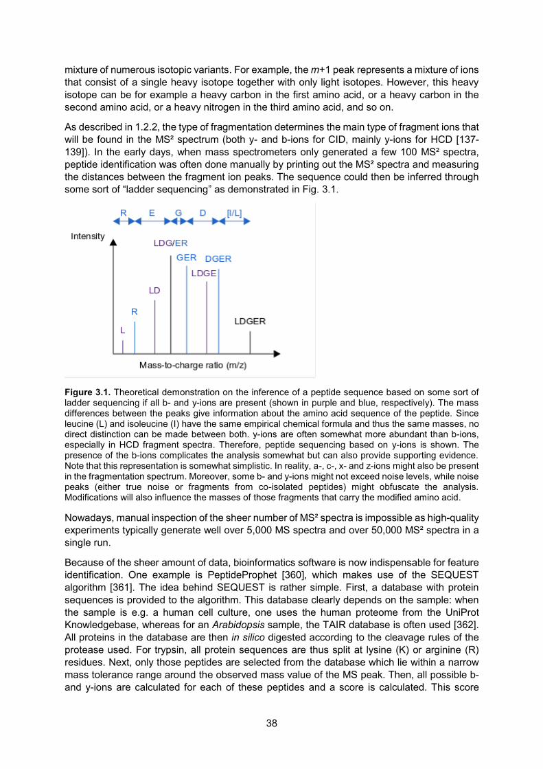
38

mixture of numerous isotopic variants. For example, the m+1 peak represents a mixture of ions that consist of a single heavy isotope together with only light isotopes. However, this heavy isotope can be for example a heavy carbon in the first amino acid, or a heavy carbon in the second amino acid, or a heavy nitrogen in the third amino acid, and so on.

As described in 1.2.2, the type of fragmentation determines the main type of fragment ions that will be found in the MS² spectrum (both y- and b-ions for CID, mainly y-ions for HCD [137-139]). In the early days, when mass spectrometers only generated a few 100 MS² spectra, peptide identification was often done manually by printing out the MS² spectra and measuring the distances between the fragment ion peaks. The sequence could then be inferred through some sort of “ladder sequencing” as demonstrated in Fig. 3.1.

Figure 3.1. Theoretical demonstration on the inference of a peptide sequence based on some sort of ladder sequencing if all b- and y-ions are present (shown in purple and blue, respectively). The mass differences between the peaks give information about the amino acid sequence of the peptide. Since leucine (L) and isoleucine (I) have the same empirical chemical formula and thus the same masses, no direct distinction can be made between both. y-ions are often somewhat more abundant than b-ions, especially in HCD fragment spectra. Therefore, peptide sequencing based on y-ions is shown. The presence of the b-ions complicates the analysis somewhat but can also provide supporting evidence. Note that this representation is somewhat simplistic. In reality, a-, c-, x- and z-ions might also be present in the fragmentation spectrum. Moreover, some b- and y-ions might not exceed noise levels, while noise peaks (either true noise or fragments from co-isolated peptides) might obfuscate the analysis. Modifications will also influence the masses of those fragments that carry the modified amino acid.

Nowadays, manual inspection of the sheer number of MS² spectra is impossible as high-quality experiments typically generate well over 5,000 MS spectra and over 50,000 MS² spectra in a single run.

Because of the sheer amount of data, bioinformatics software is now indispensable for feature identification. One example is PeptideProphet [360], which makes use of the SEQUEST algorithm [361]. The idea behind SEQUEST is rather simple. First, a database with protein sequences is provided to the algorithm. This database clearly depends on the sample: when the sample is e.g. a human cell culture, one uses the human proteome from the UniProt Knowledgebase, whereas for an Arabidopsis sample, the TAIR database is often used [362]. All proteins in the database are then in silico digested according to the cleavage rules of the protease used. For trypsin, all protein sequences are thus split at lysine (K) or arginine (R) residues. Next, only those peptides are selected from the database which lie within a narrow mass tolerance range around the observed mass value of the MS peak. Then, all possible b- and y-ions are calculated for each of these peptides and a score is calculated. This score

39

increases for each theoretical b- or y-ion that, again within a certain mass tolerance, can be matched to an observed MS² peak. Similarly, the score decreases for each theoretical peak that cannot be matched to an observed peak and for any observed peak that cannot be matched to a theoretical one. All theoretical peptide candidates are then ranked according to their scores and the highest-ranking peptide is assumed to be the correct one if it scores significantly higher than the second-highest ranking peptide. This coupling of a peptide ion species to a certain MS² spectrum (and hence the corresponding MS peak) is termed a peptide-to-spectrum match (PSM) [363]. The simple idea of calculating a score based on theoretical spectra from in silico digested proteins still remains the basis of all other database search algorithms today.

In reality, the SEQUEST algorithm is more complicated than described above as it also takes neutral losses such as water, ammonia and carbon dioxide into account. In its earliest version, modifications could only be considered if they were assumed to be present at every occurrence of the modification site. This was achieved by simply shifting the masses of the in silico peptides. Later on, variable modifications were also introduced. This means that the algorithm searches both for the presence and the absence of certain modifications on certain amino acids in certain peptides. Phosphorylation of serine, threonine and tyrosine residues is an example of a variable modification that is often included in a search. One problem with searching for variable modifications is that they massively inflate the computational search space, especially if peptides are allowed to carry multiple modifications at multiple amino acids. For example, a variable search for phosphorylation alone may lead to a 67-fold increase in the search space [364]. Such inflations do not only drastically increase computational search times, but also increase the uncertainty on PSMs that map to unmodified peptides because of the increased probability that an in silico spectrum of an unrelated modified peptide matches against the spectrum of an unmodified peptide. Researchers are therefore often advised to not search for more than two or three variable modifications. Nonetheless, search space inflation can be largely fended off with some clever optimizations because the masses of modifications rarely coincide with amino acid masses, a property that can be exploited in high-resolution MS data [365]. Other optimizations include performing a two-pass search in which the second search only probes for modifications of peptides for which an unmodified counterpart was already identified in the first search [366]. Alternatively, one could limit the search to those modifications and modification sites that have previously been confirmed and are stored in a curated database [364]. Interestingly, it has been shown that unaccounted modifications are responsible for about 20–50% of all false positive identifications [367]. Therefore, open modification search engines have been developed that allow users to search for mass differences [365]. That way, much more modifications and even peptides that differ by a single amino acid from the canonical sequence in the database can be detected.

The Mascot search engine was the first to introduce probability-based scoring, whereby the probability of an identification was weighted against the probability that a match between the theoretical and the observed spectrum occurred by random chance [368]. This was later on improved by incorporating the concept of target-decoy matching [369, 370]. In target-decoy matching, a set of nonsensical peptides (decoys) of the same size as the theoretical database peptide set (targets) is added to the search space. This nonsensical set can be obtained in multiple ways, e.g. by random scrambling of the original protein sequences, but is mostly obtained by simply reversing the protein sequences followed by in silico digestion. In case of palindromic sequences, forward and reverse sequences would overlap, but palindromes are extremely rare in practice because the protease’s specificity typically requires peptides to end in very few specific amino acids (e.g. arginine (R) or lysine (K) in the case of trypsin). Therefore, a palindromic sequence should already display a missed cleavage after the first amino acid, which is rather uncommon. Next, the observed peaks are matched against the combined

40

database as described before. Then, an identification false discovery rate (FDR) threshold is calculated for each target-PSM. This FDR is simply calculated by dividing the number of equally- or higher-scoring decoy-PSMs by the number of equally- or higher-scoring target-PSMs. Finally, an FDR threshold is set (typically at 1%, rarely at 5%) and all PSMs under this threshold are passed on to the quantification stage, while the PSMs that exceed the threshold are removed from the data as these are deemed not certain enough. Note that for two-pass searches, this FDR calculation is way too liberal because the enrichment of targets in the first pass makes it more likely for the spectra to match to targets in the second pass. This constitutes a violation of the assumption that false matches should be equally likely to match a target or a decoy. Therefore, two-pass searches require an adjusted target-decoy database [371].

Nowadays, there are many different algorithms that enable peptide identifications from MS² spectra. These include Tide, a fast implementation of the SEQUEST algorithm [372], X!Tandem [373], MS-GF+ [374], MS Amanda [375], MyriMatch [376], Comet [377], Andromeda [378], OMSSA [379], Novor [380] and DirecTag [381]. A tool like SearchGUI [382], developed by the compOmics lab, unites all these algorithms in a graphical user interface. Furthermore, tools such as PeptideShaker [383] can be used to combine results of different search engines to boost identifications. The MaxQuant software package, which uses the Andromeda search engine, is very popular nowadays thanks to its integrated pipeline from identification to quantification and its user-friendly graphical user interface [384].

3.2. Protein inference In a typical shotgun proteomics workflow, the aim is to identify and quantify as many proteins as possible, but the data used for this are at the PSM level. Therefore, PSMs should be first assigned to one (or more) protein(s). Protein inference is straightforward for peptides that can be uniquely mapped to a protein sequence stored in a database. However, this becomes more complicated when a peptide can be mapped to several protein sequences [385], which frequently occurs for different protein isoforms that result from alternative splicing and for proteins that originate from paralogous genes27. Such peptides are called “shared peptides”, “degenerate peptides” or “razor peptides”.

PeptideProphet was the first algorithm to propose a solution to this problem [386]. Here, protein identification probabilities are first calculated under the assumption that all peptide matches are independent. Then, peptide identification probabilities are updated based on the protein identification probabilities. This updating of peptide and protein identification probabilities is then repeated until convergence. Others statistical models have also been proposed in an attempt to more reliably assign shared peptides [387, 388]. A conceptually simple way to deal with shared peptides is Occam’s razor approach. Here, each shared peptide is simply assigned to the protein which already has the highest number of identified unique peptides assigned to it. This is the approach currently implemented in MaxQuant [384]. MaxQuant also groups proteins that share a large fraction of their peptides in so-called “protein groups”. As the abundance of a shared peptide might reflect the combined abundance of multiple proteins, shared peptides are almost always removed from the dataset prior to quantification.

Another issue in protein inference is the occurrence of so-called “one hit wonders”: proteins that are identified by a single peptide. It is generally considered unreliable to infer a protein

27 Paralogous genes are genes that descend from the same ancestral gene within a species and therefore often

have a high sequence homology. Their resulting protein products often execute similar functions.

41

based on a single peptide because if this identification is incorrect28, a protein is quantified that might not even be present in the sample. Therefore, such proteins are often removed from the dataset after using the so-called “two-peptide rule” [385], which however has also been criticized. It was indeed shown that it is more likely to find a protein with two mediocre-scoring peptides in the decoy database than it is to find a protein with a single high-scoring peptide in the decoy database [389, 390]. It was therefore proposed to abandon this two-peptide rule in favor of an approach in which the protein identification FDR is the sole criterion to accept a protein as being identified. Indeed, although in the past, all PSMs that passed a certain FDR threshold were passed on to the quantification stage, it was soon shown that if the PSM FDR is controlled at the 1% level, the protein FDR is much higher and should therefore also be taken into account [391, 392]. This is because the chance that a false positive PSM maps to a protein in the database is in theory random and therefore only dependent on that protein’s number of theoretical (tryptic) peptides. However, a protein that is truly present in a sample will typically generate multiple PSMs that will correctly map to that protein. Therefore, a fraction of the proteins in the dataset (i.e. the true positives) will be enriched in true positive PSMs, while a relatively large fraction of false positive proteins will have very little PSMs assigned to them [393].

Many different methods have been developed to estimate protein identification FDRs [386, 394-396]. However, when calculating a protein FDR, it is important to clearly define how this value is to be interpreted. As noted by The et al. (2016), a distinction should be made between defining a false discovery as a protein that is inferred from an incorrect PSM versus defining a false discovery as the incorrect identification of a protein that is in reality not present in the sample [397]. These are not the same, as many proteins might be present in the sample that are not assigned any correct PSM but can be assigned to one or more incorrect PSMs by random chance. These authors noted that protein FDRs can strongly differ depending on the definition.

The protein inference problem is reviewed more in depth in Huang et al. (2012) [398] and Serang and Noble (2012) [399].

3.3. Peptide quantification A first step in the quantification procedure is the determination of the abundance of all identified peptides. This can be done in two ways. The first way, summing up MS² intensities, is now largely deprecated for label-free DDA data. The second and by far the most common way is by using the MS intensities.

The reason why label-free approaches in which MS² fragment ion intensities are summed to determine a peptide ion’s intensity perform worse than MS peak-based methods in terms of reproducibility, missing data, quantitative dynamic range and quantitative accuracy [307] is because MS² intensities are highly data-dependent. Due to dynamic exclusion, a particular peptide ion can be targeted for fragmentation when it is relatively far from its elution apex. This makes summed-up MS² intensities much more variable from run to run and hence less suited for reliable quantification.

When quantifying peptides based on MS intensities, it is important to realize that peptides elute continuously from the RP-HPLC column, while MS spectra are recorded at discrete time points. Indeed, if an MS spectrum is recorded every second and peptide elution typically ranges from 5-25 seconds [325, 326], most peptide ion peaks will be recorded in multiple, sequential MS 28 At a 1% PSM identification FDR, on average 1% of all PSMs is expected to be wrong, but for each specific PSM,

this probability might be significantly higher or lower.

42

spectra (see also 2.2.2). Here, every peptide ion is recorded in each MS spectrum as an isotopic envelope due to the natural isotopic occurrence. A simple way to determine an identified peptide ion’s intensity would be to sum the intensities of the isotopic envelopes in each MS spectrum and select the MS spectrum in which this summed intensity is the highest (i.e. near the peptide’s elution peak). However, this results in rather imprecise quantifications because for one peptide ion, an MS spectrum might be recorded very close to its elution peak, while for another ion, the MS spectrum with the ion’s highest intensity peak might be recorded up to 0.5 seconds29 before or after its elution peak. As shown in Fig. 3.2, the elution profile of a peptide can be fairly easily reconstructed based on the sampled MS intensities of this peptide. Indeed, by fitting a curve to these summed intensities over time, a peptide’s elution profile can be reconstructed, which results in a much more reproducible quantification [400, 401].

Figure 3.2. Theoretical example demonstrating the challenges in MS1 and MS² peptide quantification. A. Illustration of the elution profile of three peptides (blue, red and green). Arrows denote the discrete time points at which an MS spectrum is taken. Crosses on the elution profile indicate when that specific peptide is selected for fragmentation, which results in an MS² spectrum. MS spectra at time points a, b and c are shown in B; MS² spectra are shown in C. Due to its high abundance, the blue peptide was selected for fragmentation early in its elution profile (MS² spectrum d: dark blue). Because of dynamic exclusion, this peptide was not re-selected for fragmentation again until far beyond its elution peak (MS² spectrum f: light blue). Reprinted with permission from Krey et al. (2014) [402], © 2014 American Chemical Society.

Some methods are even more sophisticated in trying to increase the quantitative accuracy. For example, the Andromeda search engine, incorporated in MaxQuant, integrates the peak intensities of each ion’s isotopic envelope during peptide elution. More specifically, Andromeda fits a Gaussian peak to the three most central data points in each isotopic envelope. These 2D peaks are then smoothed to 3D peaks in the retention time dimension and the total intensity for a particular ion is then set equal to the volume of its corresponding 3D peak [384]. Fig. 3.3 gives a 3D visualization of the increase in intensities in the isotopic envelope at the start of the elution of a peptide ion.

29 This is, given that an MS spectrum is recorded every second, a typical user-defined setting.

43

Figure 3.3. 3D view of the isotopic peaks during the elution of the doubly charged peptide ion CCSDVFNQVVK in sequential MS spectra in the MaxQuant Viewer tab. Image adapted from Tyanova et al. (2015) [403]. Proteomics. Published by Wiley‐VCH Verlag GmbH & Co. KGaA, Weinheim, CC BY-NC-ND 4.0.

A disadvantage of Andromeda’s algorithm is that it is computationally intensive. Moreover, until very recently, MaxQuant was only available on Windows, which impeded its inclusion in automated Linux server pipelines [404]. These were the main motivations for the development of moFF, a platform-independent quantification algorithm that only quantifies the apex of the elution profile, making it fast, but without compromising on quality [405, 406]. Do note that many other algorithms have been developed to calculate peptide ion intensities, some of which are reviewed in Sandin et al. (2014) [407].

3.4. The nature of the data The previously described workflow results in specific data properties that are typical for MS-based proteomics and that are important to bear in mind when evaluating protein levels.

In bottom-up proteomics, PSMs do not correspond to peptides, but to peptide ions, whereby multiple peptide ions can map to the same peptide sequence. Indeed, the same peptide can often be identified under different charge states and/or with different modifications. Sometimes, a given modification can be detected at more than one location within the same peptide. As the (unmodified) backbone amino acid sequences of such PSMs are identical, these ion species are expected to behave more alike compared to unrelated ion species. Therefore, the intensities of these species are correlated with each other. Similarly, ion species of the same charge states will also be correlated. On a higher level, there is correlation between all peptides that are mapped to the same protein. The highest level in the hierarchy is the correlation between proteins. Indeed, since proteins interact with each other in numerous pathways, proteins that closely interact with each other, that are part of the same signaling pathway or even reside in the same subcellular location tend to behave more similarly than totally unrelated proteins. Orthogonal to the correlations between peptides and proteins, there is a strong within-run correlation due to the relatively large run-to-run variability in label-free proteomics. To keep this run-to-run variability minimal, it is necessary to tightly control the

44

instrumentation. This makes raw label-free proteomics data hierarchical with correlations on many levels in the data. Moreover, it is possible that for the same protein in the same MS run, e.g. two peptides are observed with only one PSM, three peptides with two PSMs and one peptide with three PSMs.

Even for peptides originating from the same protein, differences in intensities are often substantial. One reason for this is that differences in proteolytic cleavage efficiency cause some peptides to be generated more efficiently than others, rendering individual peptide levels not equal to protein levels. Moreover, intensities of different peptide ions also strongly differ because of large differences in ionization efficiency. Finally, the latter is context-dependent as the nature and the amount of co-eluting peptides also drive the efficiency by which a peptide is ionized (see chapter 8). Such ionization competition can be a more important driver of a peptide’s intensity than its actual abundance [408]. As noted in section 3.2, the intensities of shared peptide sequences arise from an unknown combination of peptide ions coming from different proteins. Therefore, shared peptides are often removed from the dataset prior to quantification.

While the raw data is at the PSM-level, quantification is typically done at the protein level. PSM-level data thus needs to be summarized to the protein level. It is possible to summarize the PSMs directly to the protein level. However, this might be suboptimal because of the hierarchical nature of the data and the missing values that make the data unbalanced. Indeed, if the PSMs would be summarized as if they were independent observations, a bias will be introduced because some peptides will be “overrepresented” in the protein’s abundance estimate, while other peptides will be “underrepresented”. Therefore, summarization is sometimes done in two steps: in a first step, the data are summarized to the peptide level (i.e. each peptide sequence is the summary of all its potential charge states and peptideforms). MaxQuant, for example, outputs peptide-level summaries as summed raw PSM intensities. In a second step, the peptide-level data are summarized to the protein level (discussed in detail in 4.1.5). Contrary to protein summarization based on peptide-level values, PSM to peptide summarization has not been studied in detail, and commonly-used data analysis pipelines such as the MaxLFQ algorithm in MaxQuant [317] and MSstats [409] calculate protein-level summaries based on PSM intensities, ignoring possible correlation between PSMs that map to the same peptide sequence. From here on, I will assume that all data are summarized to the peptide level, unless specifically mentioned otherwise. However, note that all of the criticisms regarding peptide-to-protein summarization outlined in 4.1.5 can also be applied to PSM to peptide summarization.

The linear dynamic range of the mass spectrometer also affects the data. Indeed, within a certain concentration range, an increase in peptide concentration will result in a multiplication of the MS signal with more or less the same factor. This range is termed the linear dynamic range. Above this range, the ESI spray ionization and/or the MS detector becomes saturated, leading to a plateau in the ion’s MS intensity signal. Below the linear dynamic range, a peptide ion will not be observed. Note that the linear dynamic range will be different from peptide to peptide due to their different ionization efficiencies. Fig. 3.4 gives a graphical representation of the linear dynamic range.

45

Figure 3.4. The concept of linear dynamic range in proteomics. (a) Peptide ion intensities for three theoretical proteins: a low abundant, middle abundant and highly abundant protein. For the low abundant protein, many of its peptides will fall below the limit of detection (LOD) and will therefore not be identified. Its abundance will only be estimated based on the identified peptides and might therefore be over-estimated. For the middle abundant protein, most of its peptides are observed and the protein’s estimated abundance will be close to its true abundance. For the highly abundant protein, some of its peptides will be more abundant than the upper limit of quantification (ULOQ), and their ion signals will be lowered. Hence, the highly abundant protein’s abundance might be under-estimated. (b) The dynamic range in practice. In this experiment, different known amounts of proteins were compared to each other. When the differences in concentration become large, the difference between the estimated protein abundances and the true protein abundances also increase. Such deviations from linearity are substantial for large differences in abundance. Image (a) modified after Jarnuczak et al. (2016) [330], © 2016 by American Chemical Society (“ACS”), CC BY 4.0 and image (b) adapted from Arsova et al. (2012) [410] © 2012 by The American Society for Biochemistry and Molecular Biology, Inc.

The large amount of missing values in the data is a major issue in label-free DDA shotgun proteomics. Upon searching the public repository PRIDE [411] for MaxQuant datasets that applied shotgun proteomics to full or partial proteomes, we found 16 to 82% missing values at the peptide level (see chapter 10). There are multiple reasons for this missingness. A first reason is that a protein might simply not be present in certain samples. A second reason is that experimental reasons (e.g. different tissues with different protein abundance profiles are compared), biological reasons (e.g. downregulation or degradation of a protein) or technical reasons (e.g. inferior quality of a certain run) might cause the MS intensity of a peptide that is truly present to fall below the background noise level. For label-free shotgun proteomics, the limit of detection was estimated to lie around 1 fmol [412]. A third important reason is in the data-dependent nature of the sampling: a peak that was selected in one run, might not be selected for fragmentation in a next run. Indeed, the height of the peak mainly dictates if a peak is targeted for fragmentation or not [413]. This type of missingness is thus largely intensity-dependent, although ionization also renders this type of missingness context-dependent. A fourth reason for missing values in label-free shotgun proteomics is that on average around 75% of all MS² spectra is not identified [414]. This happens when an MS² spectrum’s highest-scoring PSM falls below the pre-set identification FDR threshold or when no distinction can be made between two or more high-scoring alternatives. Alternatively, the PSM could pass the FDR threshold but might in reality be misidentified. Poorly ionizing peptides are particularly at risk for failed or incorrect identifications. Peptides carrying a phosphate-modification, for example, ionize notoriously poorly because of the phosphoryl group’s default double negative charge state. Moreover, CID fragmentation of peptides with a phosphorylated serine residue often results in a dominant neutral loss of phosphoric acid, leaving too little energy for the efficient fragmentation of the precursor’s peptide bonds [415]. Furthermore, most peptide modifications with a biological or an artefactual origin are often unsearched for due to the

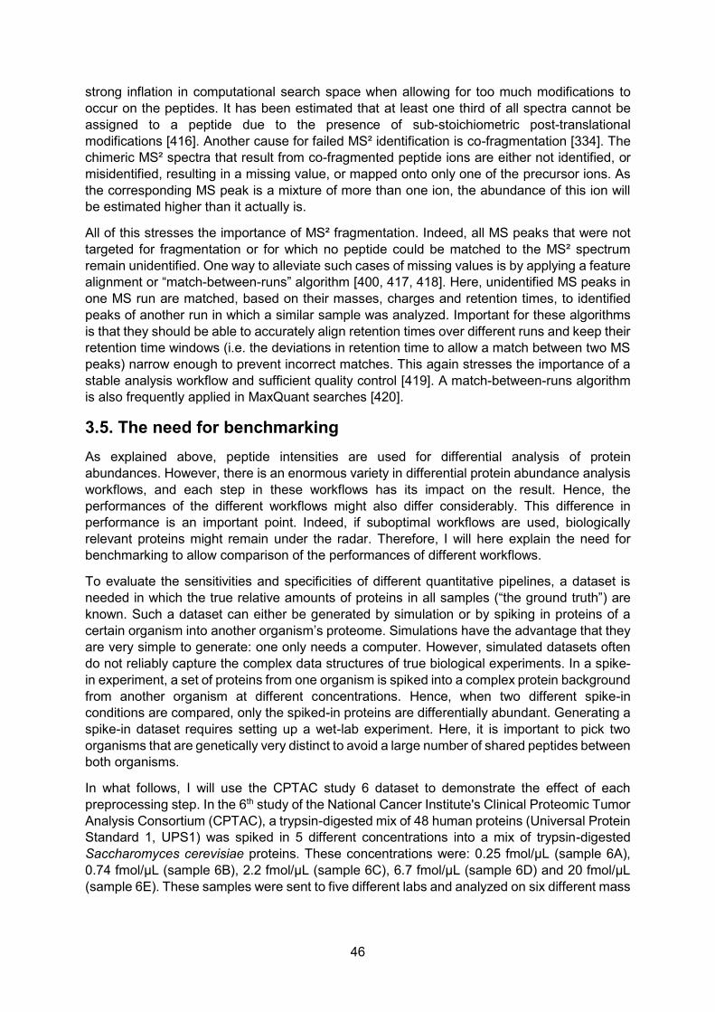
46

strong inflation in computational search space when allowing for too much modifications to occur on the peptides. It has been estimated that at least one third of all spectra cannot be assigned to a peptide due to the presence of sub-stoichiometric post-translational modifications [416]. Another cause for failed MS² identification is co-fragmentation [334]. The chimeric MS² spectra that result from co-fragmented peptide ions are either not identified, or misidentified, resulting in a missing value, or mapped onto only one of the precursor ions. As the corresponding MS peak is a mixture of more than one ion, the abundance of this ion will be estimated higher than it actually is.

All of this stresses the importance of MS² fragmentation. Indeed, all MS peaks that were not targeted for fragmentation or for which no peptide could be matched to the MS² spectrum remain unidentified. One way to alleviate such cases of missing values is by applying a feature alignment or “match-between-runs” algorithm [400, 417, 418]. Here, unidentified MS peaks in one MS run are matched, based on their masses, charges and retention times, to identified peaks of another run in which a similar sample was analyzed. Important for these algorithms is that they should be able to accurately align retention times over different runs and keep their retention time windows (i.e. the deviations in retention time to allow a match between two MS peaks) narrow enough to prevent incorrect matches. This again stresses the importance of a stable analysis workflow and sufficient quality control [419]. A match-between-runs algorithm is also frequently applied in MaxQuant searches [420].

3.5. The need for benchmarking As explained above, peptide intensities are used for differential analysis of protein abundances. However, there is an enormous variety in differential protein abundance analysis workflows, and each step in these workflows has its impact on the result. Hence, the performances of the different workflows might also differ considerably. This difference in performance is an important point. Indeed, if suboptimal workflows are used, biologically relevant proteins might remain under the radar. Therefore, I will here explain the need for benchmarking to allow comparison of the performances of different workflows.

To evaluate the sensitivities and specificities of different quantitative pipelines, a dataset is needed in which the true relative amounts of proteins in all samples (“the ground truth”) are known. Such a dataset can either be generated by simulation or by spiking in proteins of a certain organism into another organism’s proteome. Simulations have the advantage that they are very simple to generate: one only needs a computer. However, simulated datasets often do not reliably capture the complex data structures of true biological experiments. In a spike-in experiment, a set of proteins from one organism is spiked into a complex protein background from another organism at different concentrations. Hence, when two different spike-in conditions are compared, only the spiked-in proteins are differentially abundant. Generating a spike-in dataset requires setting up a wet-lab experiment. Here, it is important to pick two organisms that are genetically very distinct to avoid a large number of shared peptides between both organisms.

In what follows, I will use the CPTAC study 6 dataset to demonstrate the effect of each preprocessing step. In the 6th study of the National Cancer Institute's Clinical Proteomic Tumor Analysis Consortium (CPTAC), a trypsin-digested mix of 48 human proteins (Universal Protein Standard 1, UPS1) was spiked in 5 different concentrations into a mix of trypsin-digested Saccharomyces cerevisiae proteins. These concentrations were: 0.25 fmol/µL (sample 6A), 0.74 fmol/µL (sample 6B), 2.2 fmol/µL (sample 6C), 6.7 fmol/µL (sample 6D) and 20 fmol/µL (sample 6E). These samples were sent to five different labs and analyzed on six different mass

47

spectrometers30. For convenience, I only used the data from the LTQ-orbitraps at sites 56, 65 and 86. The study was conceived to provide a benchmark dataset to compare the power of different approaches to detect differential abundance and it is the most well-known quantification benchmark dataset. Indeed, Paulovich et al. were cited 121 times in Scopus on February 7th, 2019.

This dataset is ideal to demonstrate the statistical concept of blocking. Indeed, a typical proteomics experiment is often restricted by spatiotemporal constraints that prevent the generation of all samples simultaneously, with the same equipment, etc. Such variation causes unwanted technical variability (noise) and makes it harder to detect the effect of interest. Blocking is the experimental design choice to assign the experimental units (e.g. MS runs) to different “blocks” (e.g. batches, periods in time) in such a way that the treatments that need to be compared are present within each block. This enables to estimate the treatment effect within each block, in which the noise is lower. Blocking is therefore a way of removing unwanted variability and thus increases the power of a statistical analysis. In the CPTAC dataset, we retained the data from three different laboratories. Since the between-lab variability is not of interest, “lab” can be considered as a blocking factor, which allows to remove the between-lab variability from the analysis.

Note that there are issues with ionization competition in the CPTAC dataset [421]. Due to the relatively high spike-in concentrations of the UPS1 mix, ionization of UPS1 peptides will partially suppress the intensities of the yeast peptides. This might lead to the false positive calling of yeast proteins as DA. We indeed noticed that most quantification methods could not control their quantification false discovery rates at the 5% level when large differences in spike-in concentrations were compared [422]. Fig. 3.5 gives an overview of CPTAC Study 6, which was used in all my first-author manuscripts.

Figure 3.5. Overview of the subset of the CPTAC Study 6 that will be used throughout this thesis. Digested human UPS1 proteins were spiked in five different concentrations (6A – 6E) into digested

30 “Lab 65” analyzed the samples on two different machines

48

yeast (Saccharomyces cerevisiae) proteome. These samples were sent to three different laboratories. Each laboratory analyzed the samples in technical triplicates.

Other, more recent spike-in datasets were published in Ramus et al. (2016) [423] and Jarnuczak et al. (2016) [330].

There might be some confusion on the usage of the term “sample”. In this section, I denoted the different spike-in conditions as “samples”, which were repeatedly analyzed. However, in a biological experiment, multiple samples will be taken for each treatment condition of interest and each of these samples will be analyzed in one or more technical replicates on the mass spectrometer. Because of the ever-increasing sequencing depth, technical replication is often omitted in modern experiments, which causes each “sample” to correspond to a single MS run. In the literature, indicators referring to “sample” or “MS run” are therefore almost always used interchangeably. To avoid confusion, I will use the terms “condition” or “treatment” to refer to the spike-in conditions from now on.

49

4. DIFFERENTIAL PROTEIN ABUNDANCE ANALYSIS

Once peptides are identified, linked to a protein and assigned an intensity value, the data can be used for the analysis of differential protein abundance. In this chapter, I will go deeper into the different steps in a typical differential protein abundance analysis workflow. I will start with data preprocessing, followed by a demonstration of the most important methods to use the preprocessed data for differential protein abundance analysis.

4.1. Preprocessing Because of the nature of the peptide-level data described in section 3.4, preprocessing is required before proteins can be quantified. There is a plethora of preprocessing workflows and many of these are often constructed ad hoc. Nonetheless, in most workflows, the data typically undergo some kind of (log-)transformation, filtering, normalization, imputation and summarization. Note that the order in which each of these preprocessing steps are executed impacts on the final results. Transformation, in principle can be executed at any stage in the preprocessing workflow, but typically occurs early because it makes the data easier to handle. Similarly, filtering is done early in the workflow to remove those observations that are deemed unreliable and/or unwanted for various reasons. Furthermore, Karpievitch et al. (2012) showed that normalization followed by imputation generally outperforms imputation followed by normalization [424]. The rationale behind this is that imputing missing values obscures possible bias trends and therefore renders normalization less efficient. Moreover, imputing missing values does not make sense when unaccounted systematic bias is still present in the data. Finally, data summarization is best done after imputation as it is much more difficult to summarize data that contains missing values [425]. Nonetheless, some workflows, such as the default MaxQuant-Perseus workflow impute the data only after summarization (see 4.1.4). In this section, I discuss each of the preprocessing steps in more detail.

4.1.1. Transformation

The distributional properties of raw intensity measurements are often unfavorable for direct statistical modeling. Therefore, nearly every quantitative proteomics workflow involves a transformation of the raw intensity values. Log-transformation is a logical choice because raw intensity and concentration measurements are often more or less log-normally distributed: their values are always positive, they are skewed to the right and their variances increase with the mean. The strong right-skewness of the raw intensities is shown in Fig. 4.1: there are many relatively low intensities and only a few very high intensities. After log-transformation, the distributions become much more symmetrical.

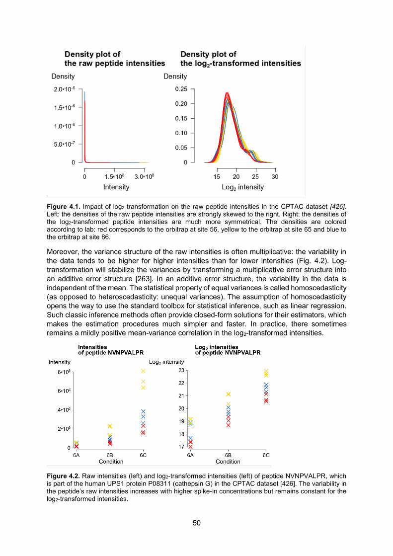
50

Figure 4.1. Impact of log2 transformation on the raw peptide intensities in the CPTAC dataset [426]. Left: the densities of the raw peptide intensities are strongly skewed to the right. Right: the densities of the log2-transformed peptide intensities are much more symmetrical. The densities are colored according to lab: red corresponds to the orbitrap at site 56, yellow to the orbitrap at site 65 and blue to the orbitrap at site 86.

Moreover, the variance structure of the raw intensities is often multiplicative: the variability in the data tends to be higher for higher intensities than for lower intensities (Fig. 4.2). Log-transformation will stabilize the variances by transforming a multiplicative error structure into an additive error structure [263]. In an additive error structure, the variability in the data is independent of the mean. The statistical property of equal variances is called homoscedasticity (as opposed to heteroscedasticity: unequal variances). The assumption of homoscedasticity opens the way to use the standard toolbox for statistical inference, such as linear regression. Such classic inference methods often provide closed-form solutions for their estimators, which makes the estimation procedures much simpler and faster. In practice, there sometimes remains a mildly positive mean-variance correlation in the log2-transformed intensities.

Figure 4.2. Raw intensities (left) and log2-transformed intensities (left) of peptide NVNPVALPR, which is part of the human UPS1 protein P08311 (cathepsin G) in the CPTAC dataset [426]. The variability in the peptide’s raw intensities increases with higher spike-in concentrations but remains constant for the log2-transformed intensities.

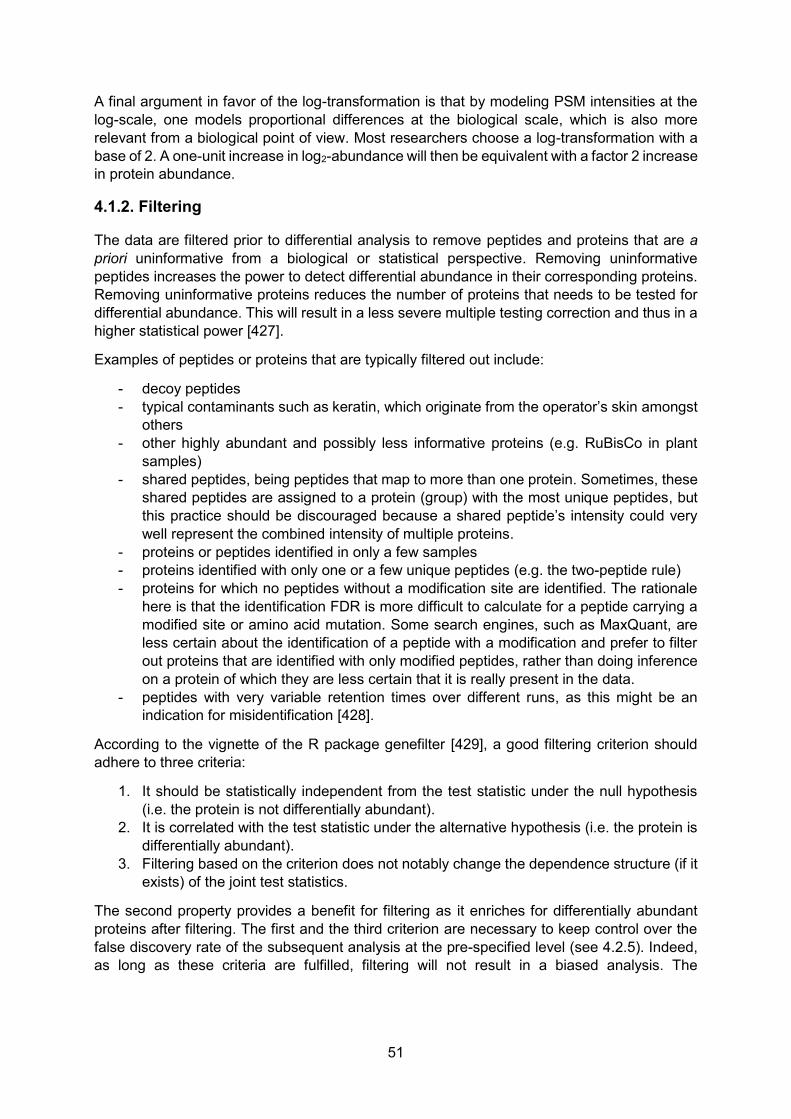
51

A final argument in favor of the log-transformation is that by modeling PSM intensities at the log-scale, one models proportional differences at the biological scale, which is also more relevant from a biological point of view. Most researchers choose a log-transformation with a base of 2. A one-unit increase in log2-abundance will then be equivalent with a factor 2 increase in protein abundance.

4.1.2. Filtering

The data are filtered prior to differential analysis to remove peptides and proteins that are a priori uninformative from a biological or statistical perspective. Removing uninformative peptides increases the power to detect differential abundance in their corresponding proteins. Removing uninformative proteins reduces the number of proteins that needs to be tested for differential abundance. This will result in a less severe multiple testing correction and thus in a higher statistical power [427].

Examples of peptides or proteins that are typically filtered out include:

- decoy peptides - typical contaminants such as keratin, which originate from the operator’s skin amongst

others - other highly abundant and possibly less informative proteins (e.g. RuBisCo in plant

samples) - shared peptides, being peptides that map to more than one protein. Sometimes, these

shared peptides are assigned to a protein (group) with the most unique peptides, but this practice should be discouraged because a shared peptide’s intensity could very well represent the combined intensity of multiple proteins.

- proteins or peptides identified in only a few samples - proteins identified with only one or a few unique peptides (e.g. the two-peptide rule) - proteins for which no peptides without a modification site are identified. The rationale

here is that the identification FDR is more difficult to calculate for a peptide carrying a modified site or amino acid mutation. Some search engines, such as MaxQuant, are less certain about the identification of a peptide with a modification and prefer to filter out proteins that are identified with only modified peptides, rather than doing inference on a protein of which they are less certain that it is really present in the data.

- peptides with very variable retention times over different runs, as this might be an indication for misidentification [428].

According to the vignette of the R package genefilter [429], a good filtering criterion should adhere to three criteria:

1. It should be statistically independent from the test statistic under the null hypothesis (i.e. the protein is not differentially abundant).

2. It is correlated with the test statistic under the alternative hypothesis (i.e. the protein is differentially abundant).

3. Filtering based on the criterion does not notably change the dependence structure (if it exists) of the joint test statistics.

The second property provides a benefit for filtering as it enriches for differentially abundant proteins after filtering. The first and the third criterion are necessary to keep control over the false discovery rate of the subsequent analysis at the pre-specified level (see 4.2.5). Indeed, as long as these criteria are fulfilled, filtering will not result in a biased analysis. The

52

aforementioned filtering procedures all fulfill the first criterion31. However, filtering on a criterion such as fold change estimates would induce a biased downstream quantification, as the fold change is an integral part of almost every test statistic and hence strongly correlates with it, also under the null hypothesis. The effect of filtering on different quantification methods has been studied in Belouah et al. (2019) [430].

4.1.3. Normalization

Even in a very clean, synthetic dataset as CPTAC, where there is no biological variability and only the spiked 48 UPS1 proteins are differentially abundant, the marginal peptide distributions are quite distinct. Considering all proteins in the dataset, there are considerable effects between samples with different spike-in concentrations, even within the same lab (Fig. 4.3, left). Moreover, for replicate measurements of the same samples, there is considerable lab-to-lab variability, and even the within-lab variability is non-negligible (Fig. 4.3, right).

Figure 4.3. Left: density plot of the log2 peptide intensities for the orbitrap at site 65 in the CPTAC dataset [426]. The densities are colored according to spike-in condition (black: spike-in condition 6A, dark red: spike-in condition 6B and green: spike-in condition 6C). Right: density plot of the log2 peptide intensities for spike-in condition 6A. The densities are colored according to lab (red: orbitrap at site 56, yellow: orbitrap at site 65 and blue: orbitrap at site 86).

Normalization aims to remove, or at least dampen, this potentially large, unwanted variability. Center mean and center median normalization subtract the respective means or medians from each distribution (Fig. 4.4). These simple normalization approaches aim to remove non-biological variability by centering the peptide intensity distributions and do not impact on their shapes [431]. However, it is clear from Fig. 4.4 that the shapes of the distributions are also affected by technical variability. Hence, more advanced normalization procedures are needed.

A method that has proven to work well for microarray data is quantile normalization [432, 433]. Quantile normalization will impose the same density distribution upon each MS-run. Here, the peptide intensities are sorted from low to high. The lowest peptide intensity for each run is then set equal to the mean of the lowest peptide intensities over these runs. Similarly, the second-lowest peptide intensity in each run will be equal to the mean of the second-lowest peptide 31 In practice, criterion 3 is rarely problematic, as most filtering procedures do not noticeably change the correlation

structure of the tests [429].

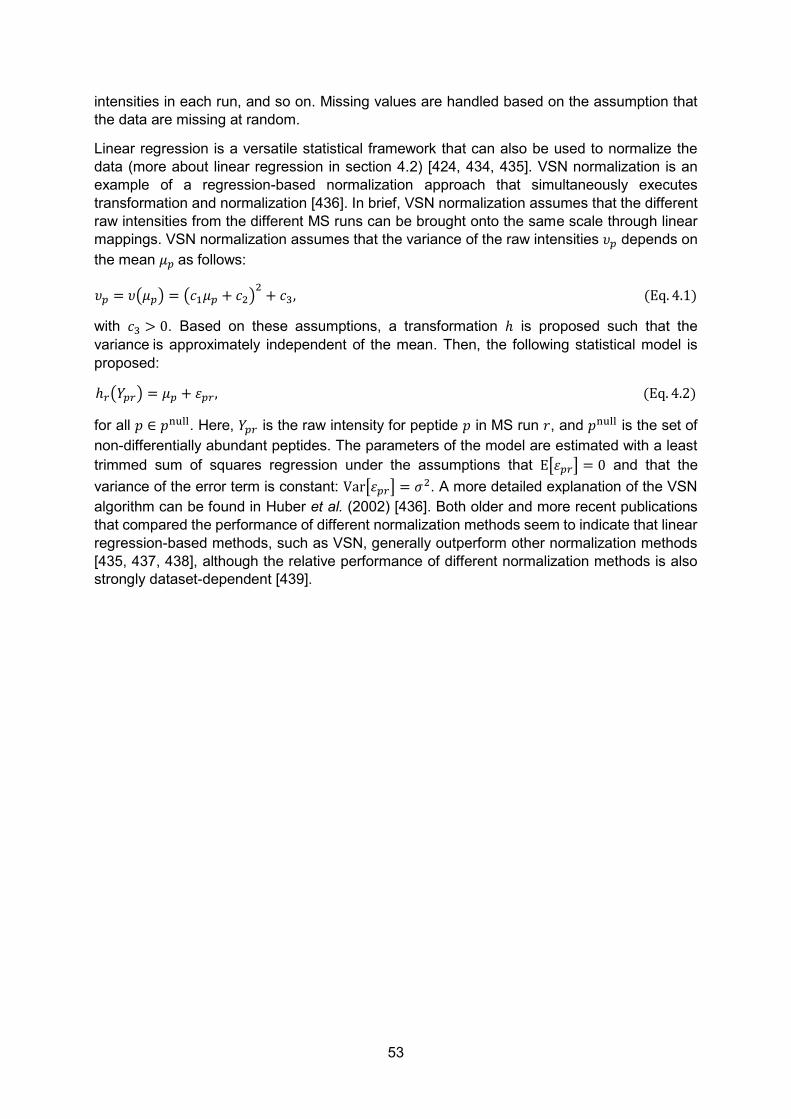
53

intensities in each run, and so on. Missing values are handled based on the assumption that the data are missing at random.

Linear regression is a versatile statistical framework that can also be used to normalize the data (more about linear regression in section 4.2) [424, 434, 435]. VSN normalization is an example of a regression-based normalization approach that simultaneously executes transformation and normalization [436]. In brief, VSN normalization assumes that the different raw intensities from the different MS runs can be brought onto the same scale through linear mappings. VSN normalization assumes that the variance of the raw intensities 𝜐𝑝 depends on the mean 𝜇𝑝 as follows:

𝜐𝑝 = 𝜐(𝜇𝑝) = (𝑐1𝜇𝑝 + 𝑐2)2 + 𝑐3, (Eq. 4.1)

with 𝑐3 > 0. Based on these assumptions, a transformation ℎ is proposed such that the variance is approximately independent of the mean. Then, the following statistical model is proposed:

ℎ𝑟(𝑌𝑝𝑟) = 𝜇𝑝 + 𝜀𝑝𝑟, (Eq. 4.2)

for all 𝑝 ∈ 𝑝null. Here, 𝑌𝑝𝑟 is the raw intensity for peptide 𝑝 in MS run 𝑟, and 𝑝null is the set of non-differentially abundant peptides. The parameters of the model are estimated with a least trimmed sum of squares regression under the assumptions that E[𝜀𝑝𝑟] = 0 and that the variance of the error term is constant: Var[𝜀𝑝𝑟] = 𝜎2. A more detailed explanation of the VSN algorithm can be found in Huber et al. (2002) [436]. Both older and more recent publications that compared the performance of different normalization methods seem to indicate that linear regression-based methods, such as VSN, generally outperform other normalization methods [435, 437, 438], although the relative performance of different normalization methods is also strongly dataset-dependent [439].

54

Figure 4.4. Overview of the effects of different types of normalization on the peptide intensity distributions in the CPTAC dataset [426].

The MaxLFQ summarization algorithm described in 4.1.5 combines summarization with normalization, although MaxLFQ summaries are sometimes still normalized afterwards.

An important assumption of all these normalization approaches is that the abundance of the large majority of the peptides remains unchanged over the different treatments. This assumption is often reasonable because researchers are mostly interested in biological perturbations that affect very specific pathways in the cell, thus affecting a minority of proteins. Moreover, most normalization methods can tolerate quite large fractions of differentially abundant peptides, as long as there is a more or less equal number of up- and downregulated peptides. This premise is also quite reasonable since the total amounts of peptides (in µg) analyzed in each run are as equal as possible.

The assumption of no major changes in the bulk of the proteome is however problematic for specific studies. For example, in AP-MS studies, proteins are purified that specifically interact with a protein of interest (bait). The control group contains only “background proteins”, i.e. proteins that non-specifically interact with the bait. Therefore, a large fraction of the identified proteins is more abundant in the samples with the bait, while the background proteins are, in

55

theory, equally abundant between control and bait samples. In such kinds of experiments, normalization should be performed with extreme caution [407].

Note that even though normalization intends to remove the overall run-to-run variability, considerable block effects can persist at the level of the individual peptides. Fig. 4.5 shows a multidimensional scaling (MDS) plot after quantile normalization for the CPTAC dataset. Even with a radical normalization method like quantile normalization, which literally forces the log2-transformed intensity distributions to be equal in each MS run, the runs clearly cluster together per lab. This demonstrates that it will be necessary to also correct for blocking effects further down the analysis pipeline.

Figure 4.5. Multidimensional Scaling (MDS) plot after quantile normalization for the CPTAC dataset [426]. The MDS plot shows each MS run in such a way that the distance between each pair of runs is equal to the root-mean-square deviation for the top 500 peptides that are the most distinct between the pairs of runs.

4.1.4. Imputation

To demonstrate the important aspects of missingness, we investigated the amount of missing values at the peptide level in 73 recent label-free shotgun proteomics datasets. We showed that on average 44% of all values at the peptide level are missing (see chapter 10). To cope with such large amounts of missing values, they are often replaced with substitute values in a process called imputation.

Classically, three types of missingness can be defined: missingness completely at random (MCAR), missingness at random (MAR) and missingness not at random (MNAR) [440]. MCAR assumes that the missing values cannot be explained by the nature of their underlying true values, nor by any known covariate: every value in the data matrix has an equal probability of being missing. MAR is a type of missingness whereby the probability of an observation to be missing is dependent on one or more observed covariates, but independent of the nature of the underlying values themselves. MNAR are all cases where the missingness is dependent on the underlying values (and optionally also on one or more known covariates): some values (e.g. very low values, very high values) have a higher probability of being missing than others.

Missingness in label-free shotgun proteomics datasets is a combination of missingness completely at random (MCAR) (e.g. an enzymatic modification in one experimental condition

56

might cause a peptide to be unidentified if that modification was not accounted for during the search), missingness at random (MAR) (e.g. certain peptide sequences ionize more easily than others; therefore, missingness is much more likely for poorly-ionizing peptides) and missingness not at random (MNAR) (e.g. more abundant peptides simply have a higher chance of getting fragmented and thus being identified). Note that this MNAR is exacerbated as the probability for a peptide to be identified is also context-dependent: when co-eluting with many other highly abundant peptides, a peptide will have a smaller chance of getting identified than if these other peptides would be absent or lower in abundance.

When choosing an imputation strategy, it is important to keep in mind the assumptions of that imputation strategy as most imputation strategies make use of either a MCAR or a MNAR assumption, but not both.

k-nearest neighbors (kNN) imputation is an example of an MCAR imputation strategy. In kNN, a Euclidean distance metric is calculated on all peptide intensities. Based on this distance matrix, the k most similar peptides (neighbors) are identified for each peptide that has at least one missing value. All missing values for that peptide are then imputed with the average of the corresponding (non-missing) values from the k neighbors [441, 442].

Quantile Regression Imputation of Left Censored data (QRILC) imputation is an example of an MNAR-based imputation strategy [443]. In QRILC, missing values are imputed with random draws from a truncated distribution with parameters that are estimated using quantile regression. QRILC has been implemented in the MSnbase R/Bioconductor package for manipulation, processing and visualization of proteomics data [444].

The popular proteomics computational platform Perseus also makes use of an MNAR-based imputation strategy. In Perseus, imputation is achieved by imputing the data with random draws from a rescaled, down-shifted normal distribution [445]. The characteristics of this distribution are calculated based on the data. More specifically, its mean is equal to the average of all the observed data minus d times the standard deviation of the observed data. Its standard deviation is equal to w times the standard deviation of the observed data. The default values for w and d are 0.3 and 1.8, respectively.

The current version of the popular Bioconductor package MSstats (version 3.12.2) [446] uses a more advanced, model-based approach to impute missing values under a MNAR assumption. Their accelerated failure time (AFT) model (see 4.2.3) does not incorporate a random missingness component as the authors argue that due to the improved technology, the proportion of random missing values has become negligible.

Choosing for no imputation, MCAR-based imputation or MNAR imputation can have a big impact on the downstream analysis. For example, the MCAR-based kNN is more suited when the majority of the missing values is not intensity-dependent [447]. Contrary, MNAR-based methods like QRILC, Perseus and AFT model imputation, perform better in a context with relatively more intensity-dependent missing values. These MNAR-based methods might however perform poorly in detecting special cases, e.g. where a long isoform of a certain protein is absent, but a smaller isoform is strongly upregulated (Fig. 4.6). In such cases, imputation with low-intensity values might dilute the signal and obscure the classification of the given protein as DA.

57

Figure 4.6. Imputation with low-intensity values can dilute signals present in the data. In this theoretical example, a protein consisting of 6 tryptic peptides is present in the left condition, while only a short isoform of the same protein giving rise to tryptic peptides 1 and 2 is 4 times more abundant in the right condition. When assessing peptides 1 and 2, the protein log2 fold change is equal to 2. However, imputing the missing values (“not assigned”, NA) with either MCAR or MNAR methods will dilute this signal.

Indeed, although imputing missing peptide values was suggested in the proteomics literature, imputation should always be used with caution. When nothing is known about the nature of the missing values, it has been suggested to use MCAR imputation approaches based on local similarity, as these perform well on average [424]. It has to be noted however, that the performance of an imputation approach is highly dataset-dependent [422, 447-449]. In reality, missing values are often caused by an unknown mix of intensity-dependent and -independent mechanisms, which is strongly dataset-specific [424, 447] and choosing the wrong imputation method for the dataset at hand can result in a severe backlash in performance [422].

Some imputation methods try to combine MCAR and MNAR imputation. For example, one of the imputation strategies in the DEP Bioconductor package by Smits and Huber suggests an imputation method whereby proteins for which the values are completely missing in one or more experimental conditions are imputed with a MNAR method, while the other missing values are imputed with a MCAR method [450]. However, this distinction is rather arbitrary, since for some proteins, all values in an experimental condition might also be missing due to random chance. Conversely, some missing values for proteins which are detected in all experimental conditions might still be due to low intensities.

A final issue with imputation is that, even if the true mechanism of missingness would be known, the uncertainty caused by replacing a missing value by a fixed value from a certain distribution is essentially ignored. A correct data analysis strategy should take this uncertainty into account. This problem might be solved by using a multiple imputation strategy [451, 452] in which the dataset is imputed multiple times and each of these imputed datasets is subsequently analyzed. The variability in the outcomes gives a good idea of the impact of the imputation on the analysis. Unfortunately, multiple imputation has not yet been widely adopted in the field. Note that it is also possible to model mechanisms of missingness explicitly (see section 4.2.3) [440].

4.1.5. Summarization

As noted in section 3.4, differential analysis mostly takes place at the protein level, but the data are at the peptide level. Therefore, most workflows involve some kind of summarization. In this section, I will focus on peptide- to protein-level summarization to show the effects of different summarization techniques. A simple way to summarize is by summing up all raw peptide intensities that correspond to each protein in each MS run [453]. Alternatively, mean summarization involves taking the mean of the peptide intensities to obtain a protein-level summary. Median summarization is also very common as a median is insensitive to outlying peptide intensities [384]. For the same reason, weighted means [454, 455] or medians [456],

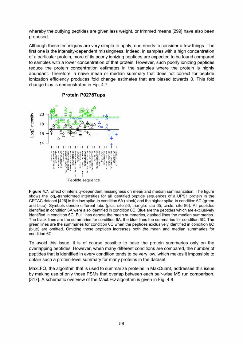
58

whereby the outlying peptides are given less weight, or trimmed means [299] have also been proposed.

Although these techniques are very simple to apply, one needs to consider a few things. The first one is the intensity-dependent missingness. Indeed, in samples with a high concentration of a particular protein, more of its poorly ionizing peptides are expected to be found compared to samples with a lower concentration of that protein. However, such poorly ionizing peptides reduce the protein concentration estimates in the samples where the protein is highly abundant. Therefore, a naive mean or median summary that does not correct for peptide ionization efficiency produces fold change estimates that are biased towards 0. This fold change bias is demonstrated in Fig. 4.7.

Figure 4.7. Effect of intensity-dependent missingness on mean and median summarization. The figure shows the log2-transformed intensities for all identified peptide sequences of a UPS1 protein in the CPTAC dataset [426] in the low spike-in condition 6A (black) and the higher spike-in condition 6C (green and blue). Symbols denote different labs (plus: site 56, triangle: site 65, circle: site 86). All peptides identified in condition 6A were also identified in condition 6C. Blue are the peptides which are exclusively identified in condition 6C. Full lines denote the mean summaries, dashed lines the median summaries. The black lines are the summaries for condition 6A, the blue lines the summaries for condition 6C. The green lines are the summaries for condition 6C when the peptides exclusively identified in condition 6C (blue) are omitted. Omitting those peptides increases both the mean and median summaries for condition 6C.

To avoid this issue, it is of course possible to base the protein summaries only on the overlapping peptides. However, when many different conditions are compared, the number of peptides that is identified in every condition tends to be very low, which makes it impossible to obtain such a protein-level summary for many proteins in the dataset.

MaxLFQ, the algorithm that is used to summarize proteins in MaxQuant, addresses this issue by making use of only those PSMs that overlap between each pair-wise MS run comparison. [317]. A schematic overview of the MaxLFQ algorithm is given in Fig. 4.8.

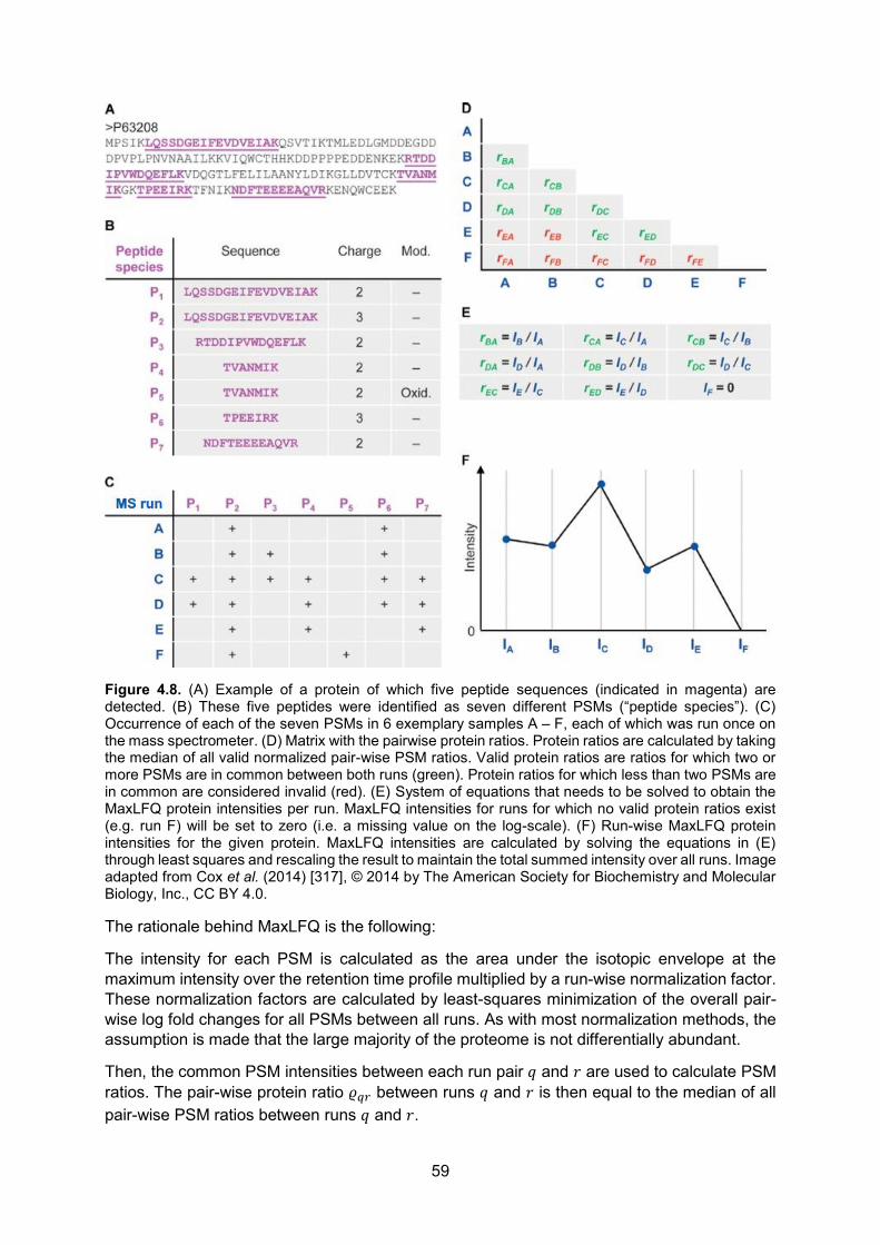
59

Figure 4.8. (A) Example of a protein of which five peptide sequences (indicated in magenta) are detected. (B) These five peptides were identified as seven different PSMs (“peptide species”). (C) Occurrence of each of the seven PSMs in 6 exemplary samples A – F, each of which was run once on the mass spectrometer. (D) Matrix with the pairwise protein ratios. Protein ratios are calculated by taking the median of all valid normalized pair-wise PSM ratios. Valid protein ratios are ratios for which two or more PSMs are in common between both runs (green). Protein ratios for which less than two PSMs are in common are considered invalid (red). (E) System of equations that needs to be solved to obtain the MaxLFQ protein intensities per run. MaxLFQ intensities for runs for which no valid protein ratios exist (e.g. run F) will be set to zero (i.e. a missing value on the log-scale). (F) Run-wise MaxLFQ protein intensities for the given protein. MaxLFQ intensities are calculated by solving the equations in (E) through least squares and rescaling the result to maintain the total summed intensity over all runs. Image adapted from Cox et al. (2014) [317], © 2014 by The American Society for Biochemistry and Molecular Biology, Inc., CC BY 4.0.

The rationale behind MaxLFQ is the following:

The intensity for each PSM is calculated as the area under the isotopic envelope at the maximum intensity over the retention time profile multiplied by a run-wise normalization factor. These normalization factors are calculated by least-squares minimization of the overall pair-wise log fold changes for all PSMs between all runs. As with most normalization methods, the assumption is made that the large majority of the proteome is not differentially abundant.

Then, the common PSM intensities between each run pair 𝑞 and 𝑟 are used to calculate PSM ratios. The pair-wise protein ratio 𝜚𝑞𝑟 between runs 𝑞 and 𝑟 is then equal to the median of all pair-wise PSM ratios between runs 𝑞 and 𝑟.

60

Based on all pair-wise protein ratios, it is then possible to calculate log-transformed protein-level intensities 𝑦𝑞 for each run 𝑞. This is done by performing the following protein-wise least-squares analyses for each “valid” pair of runs 𝑞 and 𝑟:

log 𝜚𝑞𝑟 = 𝑦𝑟 − 𝑦𝑞 + 𝜀𝑞𝑟 (Eq. 4.3)

Herein, 𝜚𝑞𝑟 is the pair-wise protein ratio between runs 𝑞 and 𝑟, 𝑦𝑞 the log-transformed protein intensity in run 𝑞 and 𝑦𝑟 the log-transformed protein intensity in run 𝑟. 𝜀𝑞𝑟 is a random error term. Pairs are considered valid if they have at least two PSMs in common. Finally, the whole profile of the estimated run intensities �̂�𝑞 is rescaled to maintain the total summed intensity for a protein over all runs. Important to note is that in this procedure, summaries are calculated solely based on the PSMs that are common between each pair of runs. Therefore, MaxLFQ does not suffer from a downwards bias in its summary estimates.

It is also possible to reformulate the summarization problem as follows:

𝑦𝑓𝑟 = 𝛽0 + 𝛽𝑓feature + 𝛽𝑟

run + 𝜀𝑓𝑟, (Eq. 4.4)

Herein, 𝑦𝑓𝑟 is the log-transformed intensity for PSM (feature) 𝑓 in run 𝑟, 𝛽0 is the intercept, which corresponds to the average log-transformed intensity of a certain reference PSM in a certain reference run. 𝛽𝑓

feature is the effect of PSM 𝑓 relative to the intercept and 𝛽𝑟run is the

effect of run 𝑟 relative to the intercept. 𝜀𝑓𝑟 is a random error term. The MaxLFQ procedure is in fact an ad hoc procedure to fit such a model for the ratio 𝑦𝑓𝑟/𝑦𝑓𝑞, conditional on all PSMs 𝑓 that are in common between runs 𝑞 and 𝑟. The disadvantage of the MaxLFQ procedure is that if the PSM overlap between runs 𝑞 and 𝑟 is very limited, the MaxLFQ estimates become very imprecise. This is the reason that MaxLFQ requires an overlap of at least two PSMs before allowing a ratio to be valid.

It is however more efficient to fit model (Eq. 4.4) as it is, as this model uses the information in all the PSMs, not only those that overlap, and still corrects for peptide-specific effects thanks to the 𝛽𝑓

feature effect. 𝛽0 + 𝛽𝑟run can then be interpreted as the average protein intensity in run

𝑟 for the reference PSM.

Median polish [457, 458] is a robust way of fitting model (Eq. 4.4) that is also implemented in the current version of MSstats, but still seems show a slightly downwards bias. MaxLFQ, conversely, produces nearly unbiased protein-level estimates (Fig. 4.9).

61

Figure 4.9. Overview of the log2 fold change estimates between condition 6C and 6A for the 36 UPS1 proteins for which these estimates could be calculated based on log2-transformed PSM-level intensities with four different summarization methods: mean summarization, median summarization, median polish and MaxLFQ. The red line denotes the true log2 fold change based on the known spike-in concentrations (2.2 fmol/µL for 6C, 0.35 fmol/µL for 6A). Mean and mean summarization strongly underestimate the true fold change. Median polish shows a smaller downwards bias, while MaxLFQ is nearly unbiased.

To avoid the downwards bias introduced by intensity-dependent missingness, MSstats imputes the data under a missing-by-low-intensity assumption prior to median polish summarization. However, such an assumption is not always valid, as already discussed in 4.1.4.

Note that both MaxLFQ and MSstats start from PSM-level intensities without taking into account the fact that PSMs mapping to the same peptide sequence are correlated.

4.2. Methods for differential protein abundance analysis Differential analysis here aims at identifying those proteins that are differentially abundant. In proteomics, there are three main methods to perform differential analysis: summarization-based methods, counting-based methods and peptide-based methods. However, differential analysis is only meaningful if the design of the study allows for it. Therefore, I will start this section with a note on the importance of the study design.

4.2.1. The importance of study design

In its early days, mass spectrometry was tedious, time-consuming and costly. The main reason for this was the low duty cycle of the mass spectrometers, implying that, within a given time frame, very few peptides got selected for fragmentation and could thus be identified. Intelligent approaches such as MudPIT [119] and ICAT [459], countered this by peptide pre-fractionation or by selecting for so-called protein-representative peptides respectively. The former increased the overall analysis time, whereas the latter relied on expensive reagents that also tended to interfere with peptide fragmentation and peptide identification. Hence, samples were often analyzed only once on mass spectrometers. Proteins were then declared “significant” solely based on a fold change threshold [241, 243]. Publications using this approach are sometimes still accepted in high-impact journals [460]. Alternatively, a normal distribution was fitted to all fold change estimates and fold changes for proteins in the upper and lower 2.5% quantiles

62

were declared “significant” [455, 461]. Some authors even developed advanced empirical Bayes methods to deal with single-run experiments [462]. However, these methods provide little to no evidence about which proteins are truly differentially abundant. Indeed, with no information on the biological variability between biological repeats, it is impossible to assess how an estimator varies from experiment to experiment. For all we know, a protein with a very high fold change estimate can be in fact a protein whose abundance is highly variable, but unrelated to the studied treatment [463]. Hence, experiments without biological repeats make it impossible to infer the results towards the population. It is thus of utmost importance to design a study in such a way that samples are included from multiple, independent subjects from the population on which one aspires to do inference. For instance, if properly conceived, a study containing only BALB/c mice should provide results that are valid for all BALB/c mice. However, if a researcher wants to extrapolate these results towards other mice strains, he or she should have included at least a few different mouse strains in his/her experimental design. Fig. 4.10 demonstrates how different levels of replication contribute to the total variability in the system.

Figure 4.10. Different levels of replication do not contribute equally and independently to the total variability in the system. In the given example, there are two biological levels of replication (animal and cell) and one technical level of replication (measurement). Although the average expression of all animals in the population is equal to 10, each of these replication levels contributes to the total measurement variability by introducing, in this example, a random error that follows a normal distribution with variances 1, 2 and 0.5 respectively (the corresponding standard deviations are shown as horizontal lines). Note that in proteomics data, these levels of replication hold for every single protein. Moreover, proteomics data has multiple levels of technical replication: MS run, peptide and PSM, as discussed in section 3.4. Reprinted with permission from Blainey et al. (2014) [464], copyright © 2014, Springer-Verlag.

Still too often, researchers limit themselves to conducting a few “biological” replicates on the same cell line, often from the same vial, or worse, they run only one sample in a few technical replicates on the mass spectrometer. In the first case, the results can only be extrapolated to that specific cell line in that specific lab, but at least, the experimental variability was taken into account (i.e. difference due to slightly different handling of the cells, a slightly different temperature because the repeats were performed on a different day, etc.). In case only technical replicates are used, the results can only be extrapolated to that specific sample.

63

These types of improper study designs are, in my opinion, one of the reasons for the replication crisis that plagues the biological sciences. An extensive overview of the statistical considerations to bear in mind when designing an MS-based proteomics experiment can be found in Oberg and Vitek (2009) [465].

4.2.2. Summarization-based methods

Summarization-based methods for differential analysis start from protein-level summaries. In this section, I will explain a few of the most commonly used methods.

Perseus is one of the most popular software packages amongst mass spectrometrists to perform differential analysis [445]. It seamlessly imports MaxQuant output and is equipped with a user-friendly GUI that allows for a variety of data manipulations, statistical analyses and visualizations.

Perseus’ default way to perform differential analysis between two groups is via t-tests on MaxLFQ-summarized, log2-transformed and preprocessed protein intensities. A t-test relies on three assumptions:

1. Independence. The information about any of the observations does not provide additional information about any of the other observations after correction for the treatment. This implies that all observations should be at the same level of hierarchy and that no pair of observations can be assumed (by design) to be more similar to each other than any other pair of observations (after correction for the treatment).

2. Normality. The normality assumption demands that the observations in both conditions are realizations of a normally distributed population.

3. Homoscedasticity. Homoscedasticity or equality of the variances means that the population variances in both conditions are equal. When the homoscedasticity assumption is not met, it is however still possible to use the Welch two-sample t-test (see below).

If the rigid assumptions of the t-test are not met, there is no guarantee that the inference will be correct. In practice, however, researchers seldom assess these assumptions, especially in high-throughput omics contexts. The rationale behind a t-test is to weigh the fold change of a protein by its natural variability in abundance. Indeed, as explained above, a high fold change is not very meaningful if a protein’s abundance is very variable from sample to sample (Fig. 4.11).

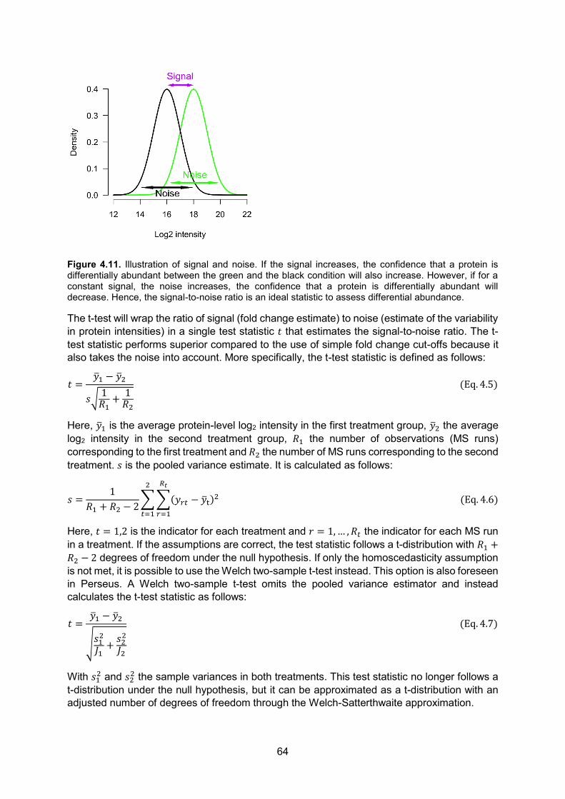
64

Figure 4.11. Illustration of signal and noise. If the signal increases, the confidence that a protein is differentially abundant between the green and the black condition will also increase. However, if for a constant signal, the noise increases, the confidence that a protein is differentially abundant will decrease. Hence, the signal-to-noise ratio is an ideal statistic to assess differential abundance.

The t-test will wrap the ratio of signal (fold change estimate) to noise (estimate of the variability in protein intensities) in a single test statistic 𝑡 that estimates the signal-to-noise ratio. The t-test statistic performs superior compared to the use of simple fold change cut-offs because it also takes the noise into account. More specifically, the t-test statistic is defined as follows:

𝑡 =�̅�1 − �̅�2

𝑠√ 1𝑅1

+ 1𝑅2

(Eq. 4.5)

Here, �̅�1 is the average protein-level log2 intensity in the first treatment group, �̅�2 the average log2 intensity in the second treatment group, 𝑅1 the number of observations (MS runs) corresponding to the first treatment and 𝑅2 the number of MS runs corresponding to the second treatment. 𝑠 is the pooled variance estimate. It is calculated as follows:

𝑠 =1

𝑅1 + 𝑅2 − 2∑∑(𝑦𝑟𝑡 − �̅�t)2

𝑅𝑡

𝑟=1

2

𝑡=1

(Eq. 4.6)

Here, 𝑡 = 1,2 is the indicator for each treatment and 𝑟 = 1,… , 𝑅𝑡 the indicator for each MS run in a treatment. If the assumptions are correct, the test statistic follows a t-distribution with 𝑅1 +𝑅2 − 2 degrees of freedom under the null hypothesis. If only the homoscedasticity assumption is not met, it is possible to use the Welch two-sample t-test instead. This option is also foreseen in Perseus. A Welch two-sample t-test omits the pooled variance estimator and instead calculates the t-test statistic as follows:

𝑡 =�̅�1 − �̅�2

√𝑠12

𝐽1+ 𝑠2

2

𝐽2

(Eq. 4.7)

With 𝑠12 and 𝑠2

2 the sample variances in both treatments. This test statistic no longer follows a t-distribution under the null hypothesis, but it can be approximated as a t-distribution with an adjusted number of degrees of freedom through the Welch-Satterthwaite approximation.

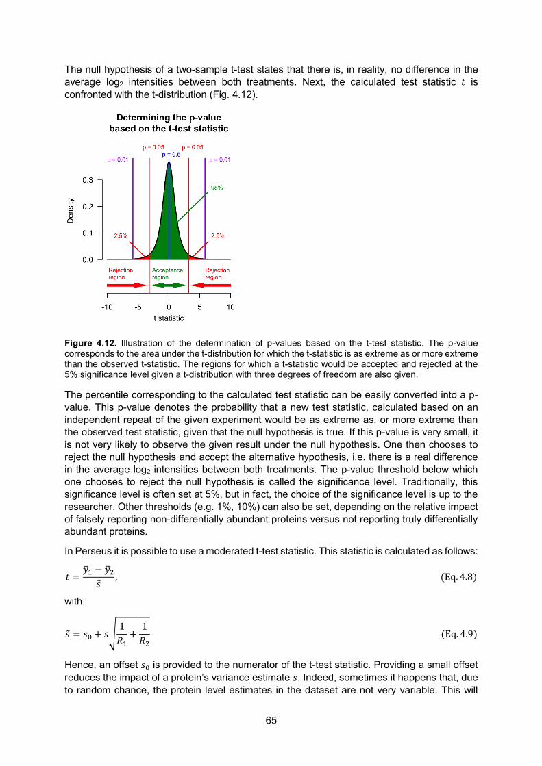
65

The null hypothesis of a two-sample t-test states that there is, in reality, no difference in the average log2 intensities between both treatments. Next, the calculated test statistic 𝑡 is confronted with the t-distribution (Fig. 4.12).

Figure 4.12. Illustration of the determination of p-values based on the t-test statistic. The p-value corresponds to the area under the t-distribution for which the t-statistic is as extreme as or more extreme than the observed t-statistic. The regions for which a t-statistic would be accepted and rejected at the 5% significance level given a t-distribution with three degrees of freedom are also given.

The percentile corresponding to the calculated test statistic can be easily converted into a p-value. This p-value denotes the probability that a new test statistic, calculated based on an independent repeat of the given experiment would be as extreme as, or more extreme than the observed test statistic, given that the null hypothesis is true. If this p-value is very small, it is not very likely to observe the given result under the null hypothesis. One then chooses to reject the null hypothesis and accept the alternative hypothesis, i.e. there is a real difference in the average log2 intensities between both treatments. The p-value threshold below which one chooses to reject the null hypothesis is called the significance level. Traditionally, this significance level is often set at 5%, but in fact, the choice of the significance level is up to the researcher. Other thresholds (e.g. 1%, 10%) can also be set, depending on the relative impact of falsely reporting non-differentially abundant proteins versus not reporting truly differentially abundant proteins.

In Perseus it is possible to use a moderated t-test statistic. This statistic is calculated as follows:

𝑡 =�̅�1 − �̅�2

�̃�, (Eq. 4.8)

with:

�̃� = 𝑠0 + 𝑠√1𝑅1

+1𝑅2

(Eq. 4.9)

Hence, an offset 𝑠0 is provided to the numerator of the t-test statistic. Providing a small offset reduces the impact of a protein’s variance estimate 𝑠. Indeed, sometimes it happens that, due to random chance, the protein level estimates in the dataset are not very variable. This will

66

result in a small pooled variance estimate 𝑠, and hence a high test statistic 𝑡 and a small p-value, even if a protein’s fold change is rather small. Such proteins, with very small fold changes, but significant p-values due to small variance estimates are often not of interest to the researcher. Adding the offset 𝑠0 stabilizes the test statistic. This procedure is known as significance analysis of microarrays (SAM) [466]. By adding the offset, the test statistic no longer follows a t-distribution and p-values are calculated by permuting the log2 protein intensities across all proteins over both treatments. The widespread use of the SAM procedure in the proteomics community, whereby 𝑠0 is arbitrarily chosen by the experimenter has been criticized as it may lead to biased quantifications [467].

The use of t-tests and SAM limits Perseus analyses only to two-group comparisons. Consider the CPTAC dataset as an illustration. When comparing condition 6C to condition 6A for example, the independence assumption of the t-test is violated. Indeed, samples that were analyzed in the same lab are more similar than samples that were analyzed in different labs. Therefore, each sample contains some information about the other samples from the same lab, thereby invalidating the independence assumption. Summarizing the data from the sample- to the lab-level seems like a solution, but besides the loss of information, this does not solve the problem that data from the same lab over different conditions are more similar than data from different labs over different conditions.

Therefore, the t-test should be expanded towards a more general framework: linear regression. In the linear regression framework, every observed outcome variable 𝑦𝑟 (with index 𝑟 = 1,… , 𝑅 denoting the MS run) is assumed to originate from a linear combination of covariates 𝑥𝑟𝑚 and regression coefficients (also termed “parameters” or “effects”) 𝛽0 and 𝛽𝑚 (with index 𝑚 =1,… ,𝑀 denoting the model parameters) summed with a random error term 𝜀𝑟 that covers the deviation of each observation 𝑦𝑟 from its expected value under the model:

𝑦𝑟 = 𝛽0 + ∑ 𝑥𝑟𝑚𝛽𝑚

𝑀

𝑚=1

+ 𝜀𝑟 (Eq. 4.10)

The linear regression model has four assumptions:

1. Independence: Independence again denotes that none of the observations holds additional information about any of the other observations after correction for the covariates 𝑥𝑟1 to 𝑥𝑟𝑀.

2. Linearity: Linearity between the response and predictors means that the outcome variable varies linearly in function of the predictors 𝑥𝑟𝑚 and that there are thus no higher-order trends that cannot be accounted for. Linearity implies that the residuals (i.e. fraction of the data that cannot be explained by the predictors) have a mean of 0 and that they are orthogonal on the predictors.

3. Normality: The errors are assumed to be normally distributed, i.e. ε𝑟~N(0, 𝜎2). 4. Homoscedasticity: Homoscedasticity requires that the variance of the residuals is equal

for each covariate pattern. This also implicates that are no trends in the spread of the residuals when the residuals are plotted in function of the fitted outcome values.

At a first glance, the linearity assumption seems to be rather restrictive for linear regression modeling. However, linear regression models can be easily adapted to capture higher-order (e.g. quadratic effects) or even non-parametric trends (e.g. splines).

Linear regression models are often written in a compact matrix notation:

𝒚 = 𝑿𝜷 + 𝜺 (Eq. 4.11)

67

For the CPTAC dataset, our aim is to compare the different conditions to each other. Therefore, separate linear regression models can be proposed for every protein 𝑖, whereby the protein-level log2 intensities are modeled in function of the spike-in conditions. By including lab effects, we also account for the blocked experimental design. As the peptide-level intensities are summarized to protein-level intensities in each run, we opt here to write an indicator 𝑟 for run instead of 𝑗 and we call 𝑅 the number of runs for which a protein-level summary could be determined for protein 𝑖. Ultimately, the matrices can be specified as follows for each protein 𝑖 in the CPTAC dataset, whereby the indicator 𝑖 is suppressed for notational convenience:

𝒚 = [

𝑦1…𝑦𝑟…𝑦𝑅

] (Eq. 4.12)

𝜷 =

[ 𝛽0

𝛽2condition

𝛽3condition

𝛽2lab

𝛽3lab ]

(Eq. 4.13)

𝑿 =

[ 𝒙𝟏…𝒙𝒓…𝒙𝑹]

=

[ 1…1…1

𝑥12condition

…𝑥𝑟2

condition

…𝑥𝑅2

condition

𝑥13condition

…𝑥𝑟3

condition

…𝑥𝑅3

condition

𝑥12lab…

𝑥𝑟2lab

…𝑥𝑅2

lab

𝑥13lab…

𝑥𝑟3lab

…𝑥𝑅3

lab] (Eq. 4.14)

𝜺 = [

𝜀1…𝜀𝑟…𝜀𝑅

] (Eq. 4.15)

Here, 𝒚 is a vector containing all log2-transformed protein-level intensities 𝑦𝑟. The vector 𝜷 contains the effect sizes: 𝛽0 is a constant intercept, which refers to the average log2-transformed protein intensity in a certain reference condition 1 (e.g. spike-in condition 6A) in a reference lab 1 (e.g. LTQ-orbitrap at site 86). 𝛽2

condition and 𝛽3condition are the effects of the

second and the third spike-in conditions relative to the reference condition after correction for lab-effects. They can be directly interpreted in terms of log2 fold changes between their corresponding spike-in condition and the condition that was chosen as a reference condition. Given a certain spike-in condition, 𝛽2

lab and 𝛽3lab denote the effects on the log2 protein intensity

of the second and the third labs, respectively, relative to the reference lab. To model the discrete, non-linear effects of spike-in condition and lab, we make use of so-called “dummy” variables whereby e.g. 𝑥𝑟2

condition is equal to 1 if run 𝑟 corresponds to the second spike-in condition and 0 otherwise. Idem for the other dummies. 𝜺, finally, is a vector that contains the random error terms 𝜀𝑟. For the CPTAC dataset, the regression model can then be written as follows:

𝑦𝑟 = 𝛽0 + ∑𝑥𝑟𝑡condition𝛽𝑡

condition3

𝑡=2

+ ∑ 𝑥𝑟𝑏lab𝛽𝑏

lab3

𝑏=2

+ 𝜀𝑟 (Eq. 4.16)

68

Regression models that contain only categorical variables32 are often presented in the more condense ANOVA notation whereby the predictor variables 𝒙𝒓 are not written explicitly, but indices are used instead to denote different levels of the categorical variable. For the CPTAC dataset, the ANOVA notation of the model can be written as follows:

𝑦𝑡𝑏𝑟 = 𝛽0 + 𝛽𝑡condition + 𝛽𝑏

lab + 𝜀𝑟 (Eq. 4.17)

Here, 𝑦𝑡𝑏𝑟 is the log2-transformed protein-level intensity for protein 𝑖 in MS run 𝑟, which corresponds to condition (treatment) 𝑡 = 2,3 and lab (block) 𝑏 = 2,3. 𝛽0 is the constant intercept. 𝛽𝑡

condition is the effect of condition 𝑡 relative to the reference condition, 𝛽𝑏lab the effect

of lab 𝑏 relative to the reference lab and 𝜀𝑟 the random error term. The estimated condition effects �̂�𝑡

condition are the effects of interest.

The most common way to estimate the parameters is by least squares, i.e. by minimizing the sum of the squared distances of the observations to the model fit:

‖𝒚 − 𝑿𝜷‖2 = (𝒚 − 𝑿𝜷)T(𝒚 − 𝑿𝜷) (Eq. 4.18)

This results in the following estimator for 𝜷:

�̂� = (𝑿𝐓𝑿)−𝟏𝑿𝐓𝒚 (Eq. 4.19)

In the least-squares context, the estimator for the variance of �̂� is given by:

Var̂(�̂�) = �̂�2(𝑿𝐓𝑿)−1 (Eq. 4.20)

Herein, �̂�2 is an unbiased estimator for the error variance:

�̂�2 =‖𝒚 − 𝑿�̂�‖

2

𝑅 − 𝑀, (Eq. 4.21)

with 𝑅 the number of runs and 𝑀 the number of estimated parameters in the mean model. The estimator for the standard error on the 𝑚th parameter estimator �̂�𝑚 can also be written as:

�̂��̂�𝑚= �̂�√𝜐𝑚, (Eq. 4.22)

with 𝜐𝑚 = (𝑿𝐓𝑿)𝑚,𝑚−1 the 𝑚th diagonal element of (𝑿𝐓𝑿)−1. Under the null hypothesis of no

differential abundance, the following test statistics follows a t-distribution with 𝑅 − 𝑀 degrees of freedom:

�̂�𝑚 − 𝑎�̂��̂�𝑚

~𝑡𝑅−𝑀 (Eq. 4.23)

Here, �̂�𝑚 is the estimated value for the 𝑚th model parameter 𝛽𝑚 (typically the effect of a certain treatment; in the case of the CPTAC study: the spike-in condition), 𝑎 the value of 𝛽𝑚 under the null hypothesis (typically zero) and �̂��̂�𝑚

the estimated variance on the estimate of 𝛽𝑚. Given the null distribution, a p-value can be calculated for each parameter, denoting its statistical significance. Note that some research questions (e.g. the difference in protein abundance between two non-reference conditions) require statistical inference on a linear combination of

32 Categorical variables are variables that do not correspond to any measurable quantities. Examples include

gender, different compounds, different treatments, etc. This is opposed to numerical variables that correspond to measurable quantities (e.g. doses of a certain compound, time after treatment, blood pressure,).

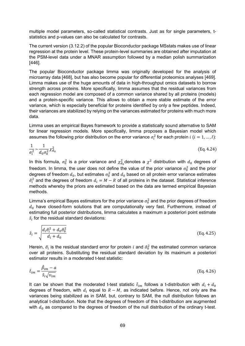
69

multiple model parameters, so-called statistical contrasts. Just as for single parameters, t-statistics and p-values can also be calculated for contrasts.

The current version (3.12.2) of the popular Bioconductor package MSstats makes use of linear regression at the protein level. These protein-level summaries are obtained after imputation at the PSM-level data under a MNAR assumption followed by a median polish summarization [446].

The popular Bioconductor package limma was originally developed for the analysis of microarray data [468], but has also become popular for differential proteomics analyses [469]. Limma makes use of the huge amounts of data in high-throughput omics datasets to borrow strength across proteins. More specifically, limma assumes that the residual variances from each regression model are composed of a common variance shared by all proteins (models) and a protein-specific variance. This allows to obtain a more stable estimate of the error variance, which is especially beneficial for proteins identified by only a few peptides. Indeed, their variances are stabilized by relying on the variances estimated for proteins with much more data.

Limma uses an empirical Bayes framework to provide a statistically sound alternative to SAM for linear regression models. More specifically, limma proposes a Bayesian model which assumes the following prior distribution on the error variance 𝜎𝑖

2 for each protein 𝑖 (𝑖 = 1,… , 𝐼):

1𝜎𝑖

2 ~1

𝑑0𝜎02 𝜒𝑑0

2 (Eq. 4.24)

In this formula, 𝜎02 is a prior variance and 𝜒𝑑0

2 denotes a 𝜒2 distribution with 𝑑0 degrees of freedom. In limma, the user does not define the value of the prior variance 𝜎0

2 and the prior degrees of freedom 𝑑0, but estimates 𝜎0

2 and 𝑑0 based on all protein error variance estimates �̂�𝑖

2 and the degrees of freedom 𝑑𝑖 = 𝑀 − 𝑅 of all proteins in the dataset. Statistical inference methods whereby the priors are estimated based on the data are termed empirical Bayesian methods.

Limma’s empirical Bayes estimators for the prior variance 𝜎02 and the prior degrees of freedom

𝑑0 have closed-form solutions that are computationally very fast. Furthermore, instead of estimating full posterior distributions, limma calculates a maximum a posteriori point estimate �̃�𝑖 for the residual standard deviations:

�̃�𝑖 = √𝑑𝑖�̂�𝑖

2 + 𝑑0�̂�02

𝑑𝑖 + 𝑑0 (Eq. 4.25)

Herein, �̂�𝑖 is the residual standard error for protein 𝑖 and �̂�02 the estimated common variance

over all proteins. Substituting the residual standard deviation by its maximum a posteriori estimator results in a moderated t-test statistic:

�̃�𝑖𝑚 =�̂�𝑖𝑚 − 𝑎�̃�𝑖√𝜐𝑖𝑚

(Eq. 4.26)

It can be shown that the moderated t-test statistic �̃�𝑖𝑚 follows a t-distribution with 𝑑𝑖 + 𝑑0 degrees of freedom, with 𝑑𝑖 equal to 𝑅 − 𝑀, as indicated before. Hence, not only are the variances being stabilized as in SAM, but, contrary to SAM, the null distribution follows an analytical t-distribution. Note that the degrees of freedom of this t-distribution are augmented with 𝑑0 as compared to the degrees of freedom of the null distribution of the ordinary t-test.

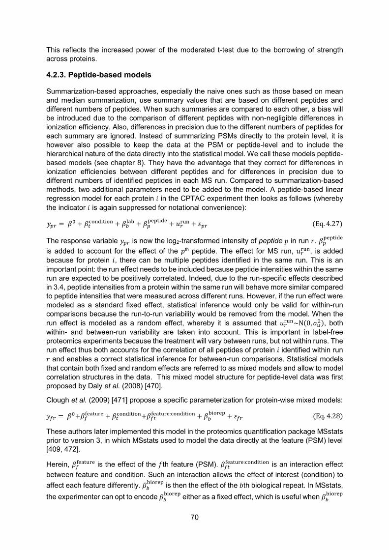
70

This reflects the increased power of the moderated t-test due to the borrowing of strength across proteins.

4.2.3. Peptide-based models

Summarization-based approaches, especially the naive ones such as those based on mean and median summarization, use summary values that are based on different peptides and different numbers of peptides. When such summaries are compared to each other, a bias will be introduced due to the comparison of different peptides with non-negligible differences in ionization efficiency. Also, differences in precision due to the different numbers of peptides for each summary are ignored. Instead of summarizing PSMs directly to the protein level, it is however also possible to keep the data at the PSM or peptide-level and to include the hierarchical nature of the data directly into the statistical model. We call these models peptide-based models (see chapter 8). They have the advantage that they correct for differences in ionization efficiencies between different peptides and for differences in precision due to different numbers of identified peptides in each MS run. Compared to summarization-based methods, two additional parameters need to be added to the model. A peptide-based linear regression model for each protein 𝑖 in the CPTAC experiment then looks as follows (whereby the indicator 𝑖 is again suppressed for notational convenience):

𝑦𝑝𝑟 = 𝛽0 + 𝛽𝑡condition + 𝛽𝑏

lab + 𝛽𝑝peptide + 𝑢𝑟

run + 𝜀𝑝𝑟 (Eq. 4.27)

The response variable 𝑦𝑝𝑟 is now the log2-transformed intensity of peptide 𝑝 in run 𝑟. 𝛽𝑝peptide

is added to account for the effect of the 𝑝th peptide. The effect for MS run, 𝑢𝑟run, is added

because for protein 𝑖, there can be multiple peptides identified in the same run. This is an important point: the run effect needs to be included because peptide intensities within the same run are expected to be positively correlated. Indeed, due to the run-specific effects described in 3.4, peptide intensities from a protein within the same run will behave more similar compared to peptide intensities that were measured across different runs. However, if the run effect were modeled as a standard fixed effect, statistical inference would only be valid for within-run comparisons because the run-to-run variability would be removed from the model. When the run effect is modeled as a random effect, whereby it is assumed that 𝑢𝑟

run~N(0, 𝜎𝑢2), both

within- and between-run variability are taken into account. This is important in label-free proteomics experiments because the treatment will vary between runs, but not within runs. The run effect thus both accounts for the correlation of all peptides of protein 𝑖 identified within run 𝑟 and enables a correct statistical inference for between-run comparisons. Statistical models that contain both fixed and random effects are referred to as mixed models and allow to model correlation structures in the data. This mixed model structure for peptide-level data was first proposed by Daly et al. (2008) [470].

Clough et al. (2009) [471] propose a specific parameterization for protein-wise mixed models:

𝑦𝑓𝑟 = 𝛽0+𝛽𝑓feature + 𝛽𝑡

condition+𝛽𝑓𝑡feature:condition + 𝛽𝑏

biorep + 𝜀𝑓𝑟 (Eq. 4.28)

These authors later implemented this model in the proteomics quantification package MSstats prior to version 3, in which MSstats used to model the data directly at the feature (PSM) level [409, 472].

Herein, 𝛽𝑓feature is the effect of the 𝑓th feature (PSM). 𝛽𝑓𝑡

feature:condition is an interaction effect between feature and condition. Such an interaction allows the effect of interest (condition) to affect each feature differently. 𝛽𝑏

biorep is then the effect of the 𝑏th biological repeat. In MSstats, the experimenter can opt to encode 𝛽𝑏

biorep either as a fixed effect, which is useful when 𝛽𝑏biorep

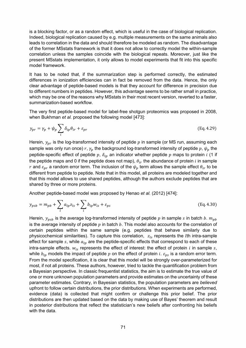
71

is a blocking factor, or as a random effect, which is useful in the case of biological replication. Indeed, biological replication caused by e.g. multiple measurements on the same animals also leads to correlation in the data and should therefore be modeled as random. The disadvantage of the former MSstats framework is that it does not allow to correctly model the within-sample correlation unless the samples coincide with the biological repeats. Moreover, just like the present MSstats implementation, it only allows to model experiments that fit into this specific model framework.

It has to be noted that, if the summarization step is performed correctly, the estimated differences in ionization efficiencies can in fact be removed from the data. Hence, the only clear advantage of peptide-based models is that they account for difference in precision due to different numbers in peptides. However, this advantage seems to be rather small in practice, which may be one of the reasons why MSstats in their most recent version, reverted to a faster, summarization-based workflow.

The very first peptide-based model for label-free shotgun proteomics was proposed in 2008, when Bukhman et al. proposed the following model [473]:

𝑦𝑝𝑟 = 𝛾𝑝 + 𝜓𝑝 ∑𝛿𝑖𝑝𝜃𝑖𝑟 + 𝜀𝑝𝑟𝑖

(Eq. 4.29)

Herein, 𝑦𝑝𝑟 is the log-transformed intensity of peptide 𝑝 in sample (or MS run, assuming each sample was only run once) 𝑟, 𝛾𝑝 the background log-transformed intensity of peptide 𝑝, 𝜓𝑝 the peptide-specific effect of peptide 𝑝, 𝛿𝑖𝑝 an indicator whether peptide 𝑝 maps to protein 𝑖 (1 if the peptide maps and 0 if the peptide does not map), 𝜃𝑖𝑟 the abundance of protein 𝑖 in sample 𝑟 and 𝜀𝑝𝑟 a random error term. The inclusion of the 𝜓𝑝 term allows the sample effect 𝜃𝑖𝑟 to be different from peptide to peptide. Note that in this model, all proteins are modeled together and that this model allows to use shared peptides, although the authors exclude peptides that are shared by three or more proteins.

Another peptide-based model was proposed by Henao et al. (2012) [474]:

𝑦𝑝𝑠𝑏 = 𝑚𝑝𝑏 + ∑𝑎𝑙𝑝𝑧𝑙𝑠 + ∑𝑏𝑖𝑝𝑤𝑖𝑠 + 𝜀𝑝𝑠 (Eq. 4.30)𝑖𝑙

Herein, 𝑦𝑝𝑠𝑏 is the average log-transformed intensity of peptide 𝑝 in sample 𝑠 in batch 𝑏. 𝑚𝑝𝑏 is the average intensity of peptide 𝑝 in batch 𝑏. This model also accounts for the correlation of certain peptides within the same sample (e.g. peptides that behave similarly due to physicochemical similarities). To capture this correlation, 𝑧𝑙𝑠 represents the 𝑙th intra-sample effect for sample 𝑠, while 𝑎𝑙𝑝 are the peptide-specific effects that correspond to each of these intra-sample effects. 𝑤𝑖𝑠 represents the effect of interest: the effect of protein 𝑖 in sample 𝑠, while 𝑏𝑖𝑝 models the impact of peptide 𝑝 on the effect of protein 𝑖. 𝜀𝑝𝑠 is a random error term. From the model specification, it is clear that this model will be strongly over-parameterized for most, if not all proteins. These authors, however, tried to tackle the quantification problem from a Bayesian perspective. In classic frequentist statistics, the aim is to estimate the true value of one or more unknown population parameters and provide estimates on the uncertainty of these parameter estimates. Contrary, in Bayesian statistics, the population parameters are believed upfront to follow certain distributions, the prior distributions. When experiments are performed, evidence (data) is collected that might confirm or challenge this prior belief. The prior distributions are then updated based on the data by making use of Bayes’ theorem and result in posterior distributions that reflect the statistician’s new beliefs after confronting his beliefs with the data.

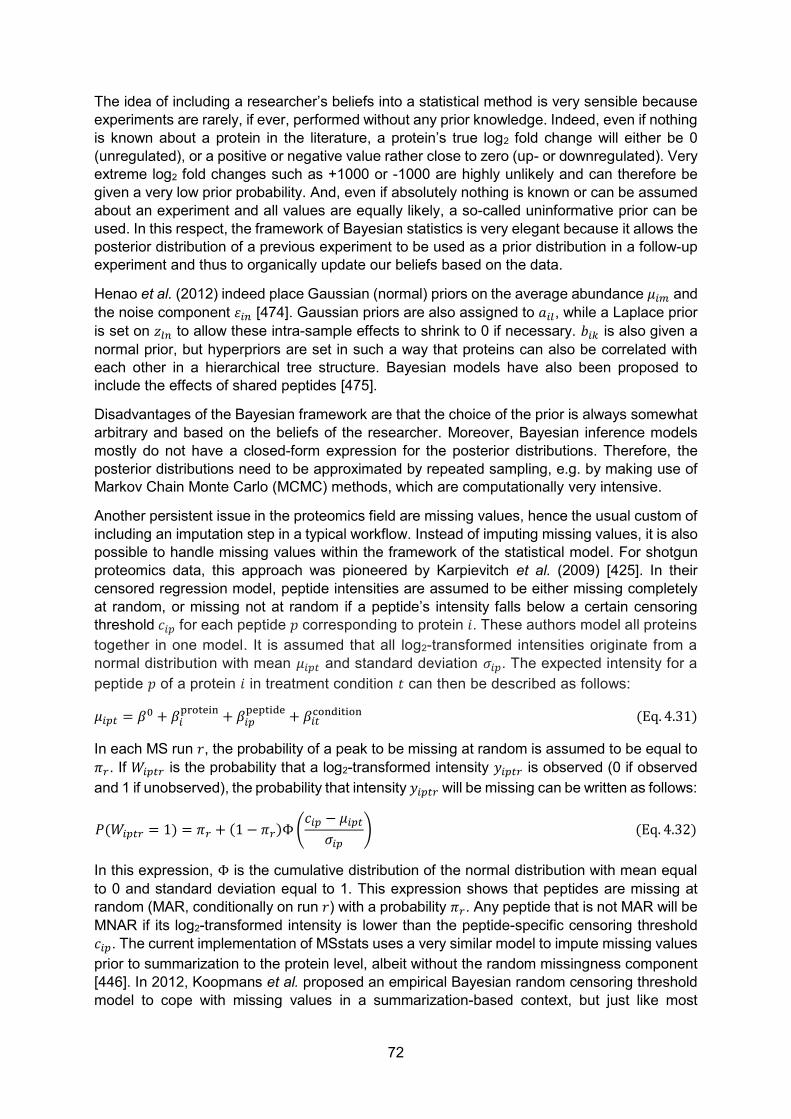
72

The idea of including a researcher’s beliefs into a statistical method is very sensible because experiments are rarely, if ever, performed without any prior knowledge. Indeed, even if nothing is known about a protein in the literature, a protein’s true log2 fold change will either be 0 (unregulated), or a positive or negative value rather close to zero (up- or downregulated). Very extreme log2 fold changes such as +1000 or -1000 are highly unlikely and can therefore be given a very low prior probability. And, even if absolutely nothing is known or can be assumed about an experiment and all values are equally likely, a so-called uninformative prior can be used. In this respect, the framework of Bayesian statistics is very elegant because it allows the posterior distribution of a previous experiment to be used as a prior distribution in a follow-up experiment and thus to organically update our beliefs based on the data.

Henao et al. (2012) indeed place Gaussian (normal) priors on the average abundance 𝜇𝑖𝑚 and the noise component 𝜀𝑖𝑛 [474]. Gaussian priors are also assigned to 𝑎𝑖𝑙, while a Laplace prior is set on 𝑧𝑙𝑛 to allow these intra-sample effects to shrink to 0 if necessary. 𝑏𝑖𝑘 is also given a normal prior, but hyperpriors are set in such a way that proteins can also be correlated with each other in a hierarchical tree structure. Bayesian models have also been proposed to include the effects of shared peptides [475].

Disadvantages of the Bayesian framework are that the choice of the prior is always somewhat arbitrary and based on the beliefs of the researcher. Moreover, Bayesian inference models mostly do not have a closed-form expression for the posterior distributions. Therefore, the posterior distributions need to be approximated by repeated sampling, e.g. by making use of Markov Chain Monte Carlo (MCMC) methods, which are computationally very intensive.

Another persistent issue in the proteomics field are missing values, hence the usual custom of including an imputation step in a typical workflow. Instead of imputing missing values, it is also possible to handle missing values within the framework of the statistical model. For shotgun proteomics data, this approach was pioneered by Karpievitch et al. (2009) [425]. In their censored regression model, peptide intensities are assumed to be either missing completely at random, or missing not at random if a peptide’s intensity falls below a certain censoring threshold 𝑐𝑖𝑝 for each peptide 𝑝 corresponding to protein 𝑖. These authors model all proteins together in one model. It is assumed that all log2-transformed intensities originate from a normal distribution with mean 𝜇𝑖𝑝𝑡 and standard deviation 𝜎𝑖𝑝. The expected intensity for a peptide 𝑝 of a protein 𝑖 in treatment condition 𝑡 can then be described as follows:

𝜇𝑖𝑝𝑡 = 𝛽0 + 𝛽𝑖protein + 𝛽𝑖𝑝

peptide + 𝛽𝑖𝑡condition (Eq. 4.31)

In each MS run 𝑟, the probability of a peak to be missing at random is assumed to be equal to 𝜋𝑟. If 𝑊𝑖𝑝𝑡𝑟 is the probability that a log2-transformed intensity 𝑦𝑖𝑝𝑡𝑟 is observed (0 if observed and 1 if unobserved), the probability that intensity 𝑦𝑖𝑝𝑡𝑟 will be missing can be written as follows:

𝑃(𝑊𝑖𝑝𝑡𝑟 = 1) = 𝜋𝑟 + (1 − 𝜋𝑟)Φ(𝑐𝑖𝑝 − 𝜇𝑖𝑝𝑡

𝜎𝑖𝑝) (Eq. 4.32)

In this expression, Φ is the cumulative distribution of the normal distribution with mean equal to 0 and standard deviation equal to 1. This expression shows that peptides are missing at random (MAR, conditionally on run 𝑟) with a probability 𝜋𝑟. Any peptide that is not MAR will be MNAR if its log2-transformed intensity is lower than the peptide-specific censoring threshold 𝑐𝑖𝑝. The current implementation of MSstats uses a very similar model to impute missing values prior to summarization to the protein level, albeit without the random missingness component [446]. In 2012, Koopmans et al. proposed an empirical Bayesian random censoring threshold model to cope with missing values in a summarization-based context, but just like most

73

Bayesian inference models, the posterior does not have a closed-form solution and needs to be constructed by repeated MCMC sampling, which makes it computationally intensive [476].

4.2.4. Ridge regression

Due to low protein abundances, limited numbers of tryptic peptides per protein and the data-dependent nature of the acquisition, the number of observed peptides is relatively small for most of the proteins in a typical label-free shotgun proteomics dataset. This makes protein-wise statistical modeling challenging because even relatively simple models are prone to over-fitting for such proteins. Over-fitting occurs when a model is too complex with respect to the amount of data that is available: the model is fit too closely to the observed data but will not generalize towards new data.

Ridge regression is a way to reduce over-fitting. Recall that for ordinary least squares, the following loss function is minimized:

‖𝒚 − 𝑿𝜷‖2 = (𝒚 − 𝑿𝜷)T(𝒚 − 𝑿𝜷) (Eq. 4.33)

Ridge regression adds a penalty term to this loss function (indicated in red):

(𝒚 − 𝑿𝜷)T(𝒚 − 𝑿𝜷) + 𝜆𝜷T𝑫𝜷, (Eq. 4.34)

with

𝐷 = [0 𝟎1×(𝑀−1)

𝟎(𝑀−1)×1 𝑰(𝑀−1)×(𝑀−1)] (Eq. 4.35)

Herein, 𝟎 is a matrix with only zeros and 𝑰 is the unit matrix33. Matrix D allows certain parameters to be unpenalized by setting their corresponding diagonal elements to 0. In the given example, only the intercept 𝛽0 remains unpenalized. The penalty term increases if the absolute values of the parameters 𝜷 increase. This prevents over-fitting by shrinking model parameters towards 0 (Fig. 4.14).

Figure 4.14. Graphical representation of the ridge estimate and the ordinary least squares (OLS) estimate in an example case where two model parameters 𝛽1 and 𝛽2 need to be estimated. The OLS

33 The unit matrix is a matrix with 1 on its diagonal elements and 0 on its off-diagonal elements. The model thus

implies equal variances for all covariates and no correlation between the covariates.

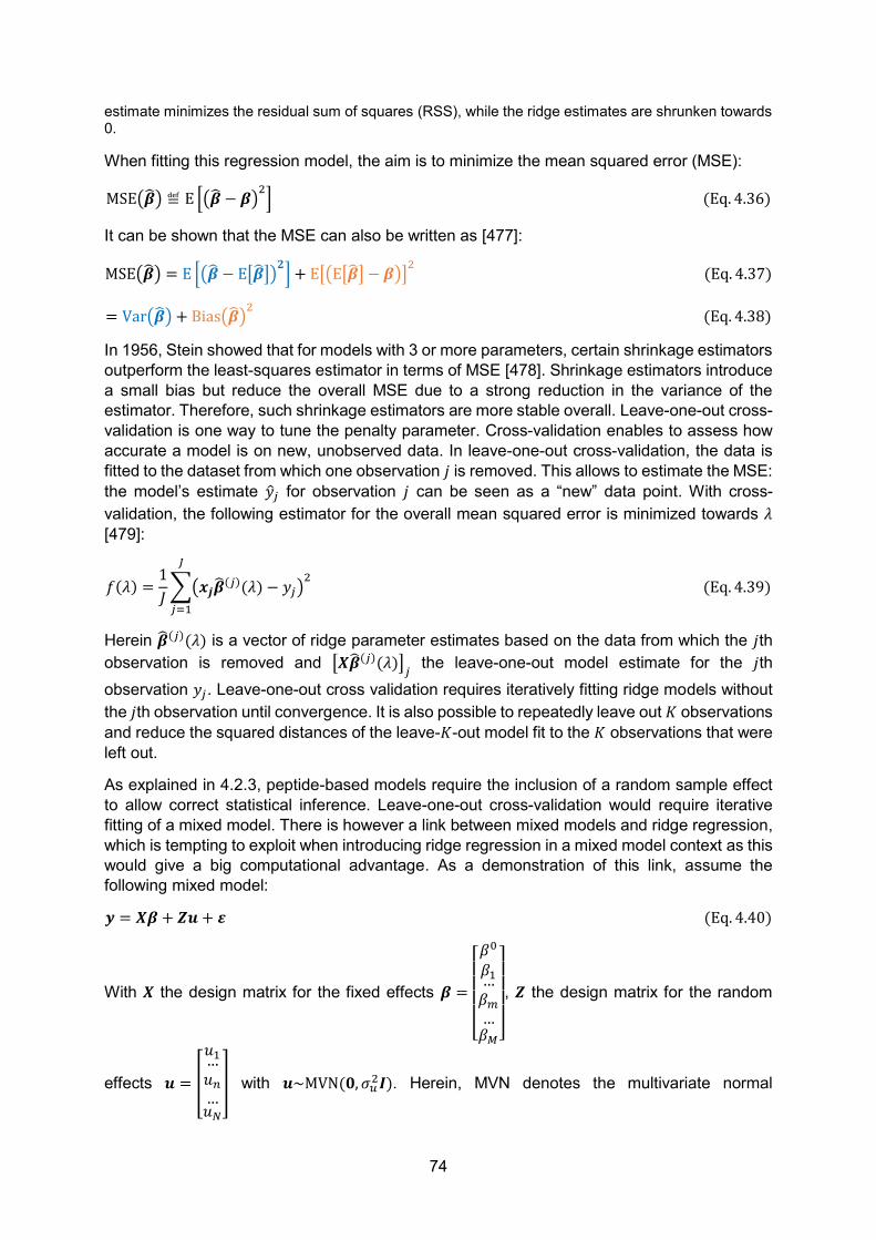
74

estimate minimizes the residual sum of squares (RSS), while the ridge estimates are shrunken towards 0.

When fitting this regression model, the aim is to minimize the mean squared error (MSE):

MSE(�̂�) ≝ E [(�̂� − 𝜷)2] (Eq. 4.36)

It can be shown that the MSE can also be written as [477]:

MSE(�̂�) = E [(�̂� − E[�̂�])𝟐] + E[(E[�̂�] − 𝜷)]

2 (Eq. 4.37)

= Var(�̂�) + Bias(�̂�)2 (Eq. 4.38)

In 1956, Stein showed that for models with 3 or more parameters, certain shrinkage estimators outperform the least-squares estimator in terms of MSE [478]. Shrinkage estimators introduce a small bias but reduce the overall MSE due to a strong reduction in the variance of the estimator. Therefore, such shrinkage estimators are more stable overall. Leave-one-out cross-validation is one way to tune the penalty parameter. Cross-validation enables to assess how accurate a model is on new, unobserved data. In leave-one-out cross-validation, the data is fitted to the dataset from which one observation 𝑗 is removed. This allows to estimate the MSE: the model’s estimate �̂�𝑗 for observation 𝑗 can be seen as a “new” data point. With cross-validation, the following estimator for the overall mean squared error is minimized towards 𝜆 [479]:

𝑓(𝜆) =1𝐽∑(𝒙𝒋�̂�(𝑗)(𝜆) − 𝑦𝑗)

2𝐽

𝑗=1

(Eq. 4.39)

Herein �̂�(𝑗)(𝜆) is a vector of ridge parameter estimates based on the data from which the 𝑗th observation is removed and [𝑿�̂�(𝑗)(𝜆)]𝑗 the leave-one-out model estimate for the 𝑗th observation 𝑦𝑗. Leave-one-out cross validation requires iteratively fitting ridge models without the 𝑗th observation until convergence. It is also possible to repeatedly leave out 𝐾 observations and reduce the squared distances of the leave-𝐾-out model fit to the 𝐾 observations that were left out.

As explained in 4.2.3, peptide-based models require the inclusion of a random sample effect to allow correct statistical inference. Leave-one-out cross-validation would require iterative fitting of a mixed model. There is however a link between mixed models and ridge regression, which is tempting to exploit when introducing ridge regression in a mixed model context as this would give a big computational advantage. As a demonstration of this link, assume the following mixed model:

𝒚 = 𝑿𝜷 + 𝒁𝒖 + 𝜺 (Eq. 4.40)

With 𝑿 the design matrix for the fixed effects 𝜷 =

[ 𝛽

0

𝛽1…𝛽𝑚…𝛽𝑀]

, 𝒁 the design matrix for the random

effects 𝒖 = [

𝑢1…𝑢𝑛…𝑢𝑁

] with 𝒖~MVN(𝟎, 𝜎𝑢2𝑰). Herein, MVN denotes the multivariate normal

75

distribution, 𝟎 a 1 × 𝑁 column vector with zeros, 𝜎𝑢2 the variance on the random effects and 𝑰

the unit matrix. 𝜺~MVN(𝟎, 𝜎2𝑰) denotes the random error terms. We maximize the joint likelihood of y, 𝜷 and 𝒖 towards 𝜷 and 𝒖:

L(𝑦, 𝜷, 𝒖) = L(𝑦, 𝜷|𝒖)L(𝒖) (Eq. 4.41)

=1

√2𝜋𝜎2𝑒−(𝒚−𝑿𝜷−𝒁𝒖)T(𝒚−𝑿𝜷−𝒁𝒖) 2𝜎2⁄ 1

√2𝜋𝜎𝑢2𝑒−(−𝒖)T(−𝒖) 2𝜎𝑢

2⁄ (Eq. 4.42)

Log-transformation results in:

l(𝑦, 𝜷, 𝒖) = −𝐽2

log(2𝜋) −𝐽2

log(𝜎2) −(𝒚 − 𝑿𝜷 − 𝒁𝒖)T(𝒚 − 𝑿𝜷 − 𝒁𝒖)

2𝜎2

−𝑁2

log(2𝜋) −𝑁2

log(𝜎𝑢2) −

𝒖T𝒖2𝜎𝑢

2 (Eq. 4.43)

With 𝑁 the number or random effect parameters. After replacing 𝜎𝑢2 by 𝜎2 𝜆⁄ and multiplying

by -2, this is equivalent with minimizing the following expression:

𝐽 log(2𝜋) + 𝐽 log(𝜎2) +(𝒚 − 𝑿𝜷 − 𝒁𝒖)T(𝒚 − 𝑿𝜷 − 𝒁𝒖)

𝜎2 + 𝑁 log(2𝜋) + 𝑁 log(𝜎2

𝜆 ) +𝜆𝒖T𝒖𝜎2

(Eq. 4.44)

Set 𝜽 = [𝜷𝒖] and 𝑪 = [𝑿 𝒁]. Minimization to 𝜽 only involves:

(𝒚 − 𝑪𝜽)T(𝒚 − 𝑪𝜽) + 𝜆𝜽T𝑫𝜽, (Eq. 4.45)

which is exactly the ridge regression loss function. Hence, parameters with a ridge penalty can be estimated by parameterizing them as random effects in a mixed model. In peptide-based models, where a random run effect needs to be included to account for within-run correlation, this link between mixed models and ridge regression can be exploited to estimate parameters with a ridge penalty, as we will see in Chapter 9.1. After optimizing the loss function, we obtain the following estimator:

�̂� = [�̂��̂�] = (𝑪T𝑪 + �̂�𝑫)

−1𝑪T𝒚 (Eq. 4.46)

This estimator for �̂� is termed the best linear unbiased predictor (BLUP). An estimate for 𝜎2 can be obtained by plugging in the estimates �̂� into the log likelihood and solving this profile log-likelihood towards 𝜎2. In practice, we make use of the restricted maximum likelihood (REML) criterion that also accounts for the degrees of freedom due to the fixed effects in the model. Conditional on 𝒖, the variance on �̂� can be estimated as follows:

Var̂ ([ �̂��̂� − 𝒖

] |𝒖) = �̂�2(𝑪T𝑪 + �̂�𝑫)−1𝑪T𝑪(𝑪T𝑪 + �̂�𝑫)

−1 (Eq. 4.47)

This variance estimator, however, does not account for the bias in the estimator �̂�. Hence, inference based on this estimator will only be correct when the bias is negligible. However, since E(𝒖) = 0, the BLUP estimator �̂� is unbiased on average over the distribution of u. Unconditional on 𝒖, the variance estimator on �̂� is given by:

Var̂ ([ �̂��̂� − 𝒖

]) = �̂�2(𝑪T𝑪 + �̂�𝑫)−1 (Eq. 4.48)

76

The estimator also accounts for the bias introduced by the penalized regression and is therefore somewhat larger than the conditional variance estimator. Ridge regression has been used in other omics fields to predict the effects of various molecular markers on organismal phenotypes [480, 481].

4.2.5. Robust regression with M estimation

Outliers are observations with extreme response values. If such observations also have a strong leverage (i.e. if they have a large distance to the average predictor values), the observation will have a strong influence on the model fit: the model will be fit close to the influential observation due to a lack of neighboring observations. Outliers are more likely to correspond to less reliable measurements. Indeed, an extremely high intensity value could for example have originated from a spike in electrospray voltage, while a very low intensity value is very likely to be missing in a repeated run due to intensity-dependent missingness. Moreover, even if the outlier is a valid measurement, it is often undesirable that a single observation has a very strong impact on the model.

Robust regression with M estimation aims to minimize the maximal bias of the estimators. With robust regression, statistical tests are only asymptotically valid. However, if the errors are normally distributed, M estimators have a high efficiency. Recall the OLS loss function:

‖𝒚 − 𝑿𝜷‖2 = (𝒚 − 𝑿𝜷)T(𝒚 − 𝑿𝜷) (Eq. 4.49)

This function is also called the L2 loss function since it minimizes the L2 norm of 𝒚 − 𝑿𝜷. With M estimation, the following loss function is minimized:

Ω(𝒚 − 𝑿𝜷) (Eq. 4.50)

The function Ω(𝑥) should have the following characteristics:

• Ω(𝑥) is symmetric • Ω(𝑥) has a minimum at Ω(0) = 0 • Ω(𝑥) is positive for all 𝑥 ≠ 0 • Ω(𝑥) increases as 𝑥 increases

Given these conditions, the estimator �̂� is the solution to the equation:

ω(𝒚 − 𝑿𝜷) = 0 (Eq. 4.51)

Where ω is the derivative of Ω. For �̂� to possess the robustness property, ω should be bounded (i.e. there exists a real number 𝑀 such that |𝜔(𝑥)| ≤ 𝑀 for all values of 𝑥). However, robust ω functions are non-linear in 𝜷 and typically do not have a closed-form solution. We will therefore recast the problem.

When location parameters 𝜷 and a scale parameter 𝜎 have to be estimated simultaneously, we minimize:

Ω(𝒚 − 𝑿𝜷

𝜎) (Eq. 4.52)

Whereby:

ω(𝒚 − 𝑿𝜷

𝜎) = 0 (Eq. 4.53)

77

Define 𝜼 = 𝒚−𝑿𝜷𝜎

and weight function 𝑤(𝜼) = ω(𝜼) 𝜼⁄ . The last estimation equation can then be rewritten as:

𝑤(𝜼)𝜼 = 0 (Eq. 4.54)

This expression can be solved as an iteratively reweighted least-squares (IRWLS) problem. Herein, the weights 𝑤(𝜼) are kept constant in 𝜼 and the expression is solved to 𝜷. Then, the weights are recalculated based on the new �̂� and the procedure is repeated until convergence.

Examples of robust loss functions Ω include:

• Huber: ΩHuber = {x2 2⁄ if |𝑥| ≤ 𝑘

𝑘(|𝑥| − 𝑘/2) if |𝑥| > 𝑘, (Eq. 4.55)

with 𝑘 = 1.345 the default tuning constant

• “Fair”: ΩFair = 𝑐2 (|𝑥|𝑐

− log (1 + |𝑥|𝑐)), (Eq. 4.56)

with 𝑐 = 1.3998 the default tuning constant • Cauchy: ΩCauchy = 𝑐2

2(1 + (𝑥 𝑐⁄ )2), (Eq. 4.57)

with 𝑐 = 1.3849 the default tuning constant

The default tuning constants are chosen in such a way that the methods have a 95% asymptotic efficiency when applied to standard normal data. Fig. 4.15 demonstrates the impact of robust regression with M estimation with Huber weights.

Figure 4.15. Plot of the residuals 𝑦𝑗 − �̂�𝑗 in function of the model-fitted values for all log2-tranformed peptide intensities �̂�𝑗 (𝑗 = 1,… , 637) of yeast protein SYKC in the CPTAC dataset after fitting regression model (Eq. 4.27) robustly with Huber weights. The sizes of the datapoints are proportional to the Huber weights in the IRWLS procedure. Note that observations with large residuals have small weights, which is indicative of the robustness property.

Examples of common loss functions and their corresponding weight functions are plotted in Fig. 4.16 and 4.17, respectively. An extensive overview of robust loss functions can be found in Bolstad (2004) [482].

78

Figure 4.16. The default L2 loss function and examples of loss functions Ω that are commonly used in robust M estimation. Figure adapted from Bolstad (2004) [482].

79

Figure 4.17. Examples of the weight functions 𝑤 that are used in the IRWL procedure to obtain the corresponding loss functions in Fig. 4.15. Figure adapted from Bolstad (2004) [482].

4.2.6. Counting-based methods

To quantify proteins with any of the above-described methods, it is necessary to extract ion intensities, which generally requires, as shown in section 3.3, rather advanced algorithms that are implemented in specialized software. Moreover, reliable protein quantification with these methods requires, depending on the study design, basic to advanced statistical knowledge. It was soon noticed that simply counting the number of MS² spectra that map to a certain protein provides a reasonably good approximation of a protein’s abundance [483, 484]. This makes sense because the more abundant a protein, the more of its peptide ions that can be expected to be detectable above noise levels. Moreover, the more abundant a peptide, the longer its elution time and hence the higher the chance that it will be targeted for fragmentation more than once, thus generating more MS² spectra. Spectral counting also deals more naturally with missing values: as a zero count [90]. Spectral counting became very appealing to many researchers, not because of its reliability, but mainly because of its ease-of-use. Indeed, researchers could now simply count the number of MS² spectra mapping to a protein and directly divide these numbers in order to obtain a fold change estimate. However, when the significance of such fold changes needs to be assessed, statistics are again needed. A natural framework for handling count data is Poisson regression. Poisson regression assumes that the spectral counts 𝑥𝑖𝑟 for each protein 𝑖 in each run 𝑟 follow a Poisson distribution:

80

𝑥𝑖𝑟~Poisson(𝜇𝑖𝑡𝑏) (Eq. 4.58)

This makes sense because a Poisson distribution is typically used to model the number of times an event occurs (detecting a spectrum that maps to protein 𝑖) during a fixed time interval (an MS run). For the CPTAC example, we can make use of the generalized linear model framework, to model the first two moments (mean and variance) of the spectral counts. As counts always have a lower bound of 0 and negative means are not meaningful for count data, we make use of a log-link function to allow unbounded estimation of the model parameters. For the CPTAC dataset, the model can be specified as follows:

log(𝜇𝑖𝑡𝑏) = 𝛽𝑖0 + 𝛽𝑖𝑡

condition + 𝛽𝑖𝑏lab (Eq. 4.59)

Note that for a Poisson distribution the mean 𝜇𝑖𝑡𝑏 and the variance 𝜐𝑖𝑡𝑏 are equal.

Here, 𝛽𝑖0 is the intercept, 𝛽𝑖𝑡

condition is the effect of spike-in condition 𝑡 and 𝛽𝑖𝑏lab is the effect of

lab 𝑏. By using a Poisson distribution, it is implied that the variance in the data 𝜐𝑖𝑡𝑏 is equal to the mean 𝜇𝑖𝑡𝑏. Such a mean-variance relationship is very restrictive. In reality, the residual variance is often larger (over-dispersion) or sometimes even smaller (under-dispersion) than what would be expected under the Poisson distribution. The mean-variance relationship can however be relaxed by making use of a quasi-Poisson regression model [485].

Note that quasi-Poisson regression does not model the full distribution, but only the first two moments of the distribution: the mean 𝜇𝑖𝑡𝑏 and the variance 𝜐𝑖𝑡𝑏. The specification of the mean model is identical to Poisson regression. However, the variance is more flexible:

𝜐𝑖𝑡𝑏 = 𝜑𝑖𝜇𝑖𝑡𝑏 (Eq. 4.60)

The factor 𝜑𝑖 allows to to correct for over- or under-dispersion. Count data can also be proposed to follow a negative binomial distribution, which assumes a quadratic mean-variance relationship:

𝜐𝑖𝑡𝑏 = 𝜇𝑖𝑡𝑏 + 𝜑𝑖𝜇𝑖𝑡𝑏2 (Eq. 4.61)

A negative binomial distribution reduces to a Poisson distribution if 𝜑𝑖 is zero. Negative binomial generalized linear models are implemented in the popular RNA sequencing quantification packages EdgeR [486, 487] and DESeq2 [488], which have also been applied in proteomics contexts [489].

Other statistical models have been proposed as well to deal with count data in proteomics, including a generalized linear mixed effects Poisson regression model in which all proteins are modeled together [490], a beta-binomial model [491] and Bayesian models [492].

Peptide counting is an alternative to spectral counting. In peptide counting, the number of unique peptides instead of the number of unique PSMs that match to each protein are counted. Some authors reported that spectral counting is more accurate and more reproducible than peptide counting which is in turn more reproducible than sequence coverage-based approaches [483, 493, 494]. This is probably because spectral counting is more fine-grained than peptide counting (there at least as much PSMs as peptides per protein), which might make it more feasible to quantify smaller differences in abundance.

A very simple peptide counting method is the Exponentially Modified Protein Abundance Index (emPAI). For each protein 𝑖, the emPAI is calculated as follows [174]:

emPAI𝑖 = 10𝑛𝑖pep 𝑛𝑖

predpep⁄ − 1 (Eq. 4.62)

81

Hereby, 𝑛𝑖pep is the number of observed unique peptides mapping to protein 𝑖 and 𝑛𝑖

predpep is the number of tryptic peptides that can theoretically map to protein 𝑖. emPAI is an example of so-called “absolute protein quantification” method. By normalizing the peptide count of each protein by its number of predicted unique tryptic peptides 𝑛𝑖

predpep, emPAI claims to be able to compare the abundances of different proteins to each other (as opposed to comparing the abundances of the same proteins over different conditions, so-called “relative quantification”). The content of protein 𝑖 in mol % is then calculated as follows:

Protein 𝑖 content (mol%) =emPAI𝑖

∑ emPAI𝑘𝑛protein𝑘=1

, (Eq. 4.63)

with 𝑛protein the total number of proteins in the dataset. Of course, for quantitative protein inference, peptide counting methods also require some statistical modeling. The models for peptide counting are very similar to those of spectral counting and many statistical models for spectral counting and peptide counting can be used interchangeably.

Absolute Protein Expression (APEX) is an example of an absolute quantification method based on spectral counting that has gained quite some traction [175, 495]. An APEX score for protein 𝑖 is calculated as follows:

APEX𝑖 =𝐶𝑛𝑖

MS2𝜋𝑖ID

𝑛𝑖predPSM ∑ 𝑛𝑘

MS2𝜋𝑘ID

𝑛𝑘predPSM

𝑛protein𝑘=1

, (Eq. 4.64)

with 𝑛𝑖MS2 the total number of MS² spectra mapping to protein 𝑖, 𝜋𝑖

ID the probability that protein 𝑖 is correctly identified, 𝑛𝑖

predPSM the number of computationally predicted PSMs for protein 𝑖 and 𝐶 an estimate of the total concentration of protein molecules in the cell.

Do note that although absolute quantification methods might give some indication about a protein’s abundance, these estimates remain generally very crude because normalizing protein abundances to each other based on e.g. the theoretical number of tryptic peptides they can generate is quite inaccurate. Also, count-based approaches have become largely obsolete in present-day proteomics given that quantification based on continuous intensity-based signals is clearly superior over discrete counts [317]. It has indeed been shown that count-based methods have a lower linear response to various protein loading amounts, a lower reproducibility, a lower quantitative accuracy, a lower precision, lower sensitivity, and a higher ratio of false positives to false negatives compared to MS intensity-based quantification [307]. This is because peptide counting disregards the inherent abundance-intensity relationship (within a certain dynamic range [496]) for each peptide. Dynamic exclusion, during which identified ions are excluded from being re-targeted for fragmentation for a certain amount of time, further obscures the relationship between spectral counts and protein abundances [497]. Counting-based approaches perform especially poorly for low-abundant proteins [228, 483, 498]. Indeed, it is not possible to calculate an accurate protein ratio between two conditions if only one or two spectra per condition are mapped to the protein of interest [497]. And, at higher levels of protein abundances, saturation effects come into play for relatively low total protein concentrations when all peptides that can theoretically be detected are in fact detected [228]. Spectral counting is reviewed extensively in Lundgren et al. (2010) [494].

4.2.7. Controlling the false discovery rate

Whether statistical inference is done with t-tests, linear regression models, or other statistical approaches, the fact that statistical inference is done for each protein in the dataset creates a

82

huge multiple testing problem. Imagine testing 1,000 proteins, all of which are not differentially abundant (i.e. the null hypothesis is true). When using the traditional 5% cut-off at the p-value level, on average 5%, i.e. 50 proteins, will be erroneously declared differentially abundant (false positives). Therefore, it is clear that, in the case of multiple testing, a significance threshold based on p-values will be way too liberal.

Solutions to this problem have been proposed in the form of controlling the family-wise error rate (FWER). The aim of FWER procedures is to control the probability of detecting at least a single false positive at a given level, typically 5%. An example of an FWER procedure is the simple, but somewhat conservative Bonferroni correction [499]. Here, a protein is only declared significantly differentially abundant if its p-value is smaller than 𝛼 𝑛protein⁄ , with 𝛼 the significant threshold (e.g. 5%) and 𝑛protein the number of proteins that are being tested. It turns out that FWER procedures are often too conservative for high-throughput applications. Indeed, the number of biological replicates in such a context is often rather low, which limits the statistical power of each individual test.

To cope with the specific context of high-throughput experiments, false discovery rate (FDR) procedures were developed. The false discovery rate aims to control the expected fraction of false positive proteins in a list of differentially abundant proteins at a certain level, again, typically 5% [500]. In practice, FDR-controlled lists are much more interesting for practitioners: a researcher will prefer a list of 20 significant proteins of which on average 1 is a false positive (i.e. the FDR is controlled at 5%) over a list of maybe 2 or 3 proteins that are not in error according to the FWER criterion. The most well-known and most widely used FDR procedure is the Benjamini-Hochberg FDR [501]. The procedure works as follows:

In a first step, the p-values are sorted from large to small. If 𝐼 p-values need to be FDR corrected, let 𝑖 = 1,… , 𝐼 be the rank of the 𝑖th p-value. Then, the q-value 𝑞𝑖 for the 𝑖th p-value is calculated as follows:

𝑞𝑖 = min𝑘

(1,𝐼𝑝𝑘

𝐼 − 𝑘 + 1) , (Eq. 4.65)

for 1 ≤ 𝑘 ≤ 𝑖. All proteins with a q-value smaller than the proposed threshold, e.g. 5%, are then considered statistically significant.

83

5. RESEARCH HYPOTHESIS

5.1. Setting the stage Many biological processes strongly depend on balanced levels of protein expression and the perturbation of a single protein can already lead to organismal malfunctioning (e.g. abnormal hemoglobin production in thalassemia [47] or extensive cellular remodeling towards a cancerous phenotype [502]). In this respect, quantitative knowledge of a proteome is very important for the unraveling of the development and progression of diseases and the identification of biomarkers, amongst others. It is fair to state that the transcriptome and the translatome only reflect the proteins that can be or are being expressed, but largely fail to provide information on a protein’s activity, function, interaction partners, localization and modification state (see 1.2.3). As proteins and their modified variants are expressed over a large concentration range, accurate quantitative information is a must to distinguish different cellular and organismal conditions [503].

Label-free shotgun proteomics leads to the identification and quantification of thousands of peptides and proteins in a single experiment. Here, analysis of differential abundance of proteins is based on ratios derived from reconstructed elution profiles based on MS intensities for all PSMs pointing to the same protein or the same protein group in a sample (see section 3.2). However, the data are highly hierarchical, and intensities can be strongly influenced by variations of peptide-specific properties. In addition, the number of peptides identified in all samples is usually limited, which leads to large numbers of missing values (Fig. 5.1), which do not occur at random. Some peptides are better detected than others and high-abundant peptide ions are more likely to yield higher numbers of fragmentation spectra. "Match between runs" algorithms can only partly compensate for this effect by reducing the number of missing values (see section 3.4).

Figure 5.12. The missing value problem. Left: the number of unique peptides identified per protein in the CPTAC dataset [426]. Right: the number of samples in which each protein in the CPTAT dataset is identified. The number of proteins identified in 9, 18 and all 27 samples are markedly elevated (cyan bars). This is because of the higher numbers of proteins that are exclusively identified in all MS runs from 1, 2 or 3 labs respectively.

Researchers have used a plethora of pipelines for the analysis of label-free shotgun proteomics data (see chapter 4). Indeed, since most mass spectrometry researchers do not have a background in statistics, different preprocessing and differential analysis methods are often combined ad hoc without a proper motivation. Many methods analyze the data protein

84

by protein by (a) filtering out proteins as soon as they are missing in a specified number of samples (see 4.1.2), (b) summarize the peptides for each protein in a sample and ignore missing values (see 4.1.5) or (c) impute missing values based on the observed peptides for the corresponding protein in other samples (see 4.1.4). Filtering out all proteins (a) leads to substantial information loss. Indeed, as demonstrated in Fig. 5.1, removing proteins that are only identified with more than a given number of peptides or requiring proteins to be identified in all of the samples would remove a substantial amount of proteins from the dataset. Summarization (b) needs to be executed such that it correctly takes the peptide-specific effects into account. A particular challenge here are the limited numbers of peptides that are identified across different samples. If summarization does not correctly take the differences in ionization efficiencies into account, it will introduce a bias because the final data will be based on different peptides. Moreover, summarization will always ignore differences in accuracy due to the different numbers of peptides on which each summary is based. Imputation (c) is even more tedious because missing values in proteomics are a combination of missing completely at random and intensity- and even context-dependent missingness. Since it is impossible to know the exact contributions of these different types of missingness, imputation according to incorrect assumptions will lead to biased quantifications. However, if missing values are simply ignored, low-abundant proteins will be over-estimated due to the limited linear dynamic range, which will reduce the power to detect differential abundance.

In addition, a proteomics experiment typically consists of a relatively small number of biological repeats compared to the large number of proteins analyzed. This gives rise to unstable variance estimates for certain proteins, especially if these proteins are identified with only a few peptides. Indeed, a small sample drawn from a given population might display a variance that is much smaller (or much bigger) than the true population variance just by random chance. Therefore, some observations might be flagged as differentially abundant solely because of their low observed variances while other truly differentially abundant proteins might be missed due to their large observed variances. This data sparsity also leads to unstable fold change estimates: one or two outlying intensities, which can for example be caused by misidentifications or co-eluting peptides, can strongly influence a protein’s fold change.

These unstable fold change and variance estimates may cause a significant increase in the number of false positives and false negatives (see e.g. the supplementary material of Doll et al. (2017) [504], where SERINC3 and PNMA1 were declared significantly altered with very weak evidence based on only a single peptide). It is therefore not surprising that a recent power calculation study on four biological repeats of Arabidopsis thaliana Col-0 samples analyzed in technical triplicate estimated that for MaxLFQ summaries, a minimal fold change of 1.4 is required to detect a statistically significant difference with 95% confidence and a power of 80%[463].

State-of-the-art proteomics quantification methods only focus on some of the sub-problems mentioned above. They generally remain fairly sensitive to outliers and correct for missing observations only to a limited extent. In addition, they usually prune the number of potential hits by filtering out proteins which have few peptides in common across the majority of the samples. Methods that model peptide-level data are often more sensitive because they naturally correct for the correlation present within the same samples, as well as for the peptide effects and the number of detected peptides for a given protein in each sample [425, 471].

Like summarization-based methods, many peptide-based models still produce unstable estimates of differential abundance and variance components due to over-parameterization. This especially occurs when few peptides are identified per protein: many low-abundant proteins are then falsely labeled as differentially abundant. Filtering on the basis of the number

85

of identified peptide spectra can provide a solution, but there is a risk that real hits will also be filtered out. Moreover, most peptide-based models remain very sensitive to outliers.

In addition, many methods are only suitable to analyze specific types of experimental designs. For example, in Perseus, it is possible to compare multiple groups to each other, but it is not possible to accurately analyze blocked designs, such as CPTAC. In MSstats, the user should annotate each experiment with a “Run”, “Condition” and “BioReplicate”. Hereby, “Run” refers to the MS run, “Condition” to the treatment of interest and “BioReplicate” to a grouping factor that is encoded as a random effect. While this set-up allows most simple experimental designs to be analyzed in a correct way, it is insufficiently flexible to correctly analyze more complicated designs with multiple confounding effects.

Finally, state-of-the-art data analysis methods, such as published models at the peptide level, do not always find their way to proteomic labs [474, 475]. This is a non-negligible problem! Indeed, many groups only demonstrated proof-of-concept, but never developed their method into a usable software package. And, those who did often lack a convenient graphical user interface that is appealing to less-experienced users. Availability, user-friendliness, documentation, support and maintenance of software tools are very important for new methods to be effective for end users.

5.2. Aims of my PhD work Based on the previous section, it is clear that state-of-the-art proteomics quantification methods do not yet make optimal use of the data, resulting in suboptimal protein quantifications. The development of robust data analysis tools for quantitative proteomics is therefore essential for the further development of the proteomics research field because, with the current data-analytical methods, many proteins remain under the radar [505]. The overall aim of my work was to develop a more robust, easy-to use proteomics quantification method that is also usable for the analysis of proteins with a limited overlap in identified peptides.

More specifically, this method should:

- account for the hierarchical nature of the data, - handle missing peptides in a more correct way, - derive strength from the massive parallel availability of peptides to estimate variance

components more correctly, - be robust to outliers, - and be able to handle complex experimental designs.

In such a method, it is important that a random effect for run is included in order to allow to correct for within-run correlation. In this respect, it is tempting to build upon the link between mixed models and ridge regression, to make use of robust regression with M estimation and to allow for empirical Bayes variance estimation. Implementing this method is expected to increase the number of truly differentially abundant proteins identified in screening experiments. The method should also be implemented and distributed in a user-friendly software tool for differential proteomics with the possibility of a graphical user interface to maximize the impact of the research.

To develop such a method, it is first necessary to thoroughly benchmark the most promising and most commonly used quantification methods. This will shed light on how preprocessing, standardization and differential analysis in a label-free proteomics quantification workflow influence a method’s performance.

87

6. OUTLINE

The remainder of my thesis is constructed as follows: first, I will present each of my published papers. In my first paper, I demonstrate how I compared different data analysis methods for differential quantification in label-free shotgun proteomics. My second paper presents the rationale behind MSqRob, the algorithm I developed to improve quantification in label-free shotgun proteomics. In my third paper, I provide a tutorial on experimental design and data analysis with MSqRob. In my fourth, unpublished paper, I make use of the additional information of peptide counts to boost MSqRob’s power and to indicate whether a protein’s significance is mainly driven by differential abundance, differential detection or both.

In the discussion, I explore the significance of my work and place it in a broader context. In the future research perspectives, I give some indications on how my research could go on from here.

89

7. REFERENCES PART I

1. Gladyshev, V.N. and G.V. Kryukov, Evolution of selenocysteine-containing proteins: Significance of identification and functional characterization of selenoproteins. BioFactors, 2001. 14(1‐4): p. 87-92.

2. Prat, L. et al., Carbon source-dependent expansion of the genetic code in bacteria. Proceedings of the National Academy of Sciences, 2012. 109(51): p. 21070-21075.

3. Koch, A. et al., A proteogenomics approach integrating proteomics and ribosome profiling increases the efficiency of protein identification and enables the discovery of alternative translation start sites. Proteomics, 2014. 14(23-24): p. 2688-2698.

4. Ruiz-Orera, J. et al., Long non-coding RNAs as a source of new peptides. eLife, 2014. 3: p. e03523-e03523.

5. Rion, N. and M.A. Rüegg, LncRNA-encoded peptides: More than translational noise? Cell Research, 2017. 27: p. 604.

6. Choi, S.-W., H.-W. Kim, and J.-W. Nam, The small peptide world in long noncoding RNAs. Briefings in Bioinformatics, 2018: p. bby055-bby055.

7. Gebert, L.F.R. and I.J. MacRae, Regulation of microRNA function in animals. Nature Reviews Molecular Cell Biology, 2019. 20(1): p. 21-37.

8. Bhat, S.A. et al., Long non-coding RNAs: Mechanism of action and functional utility. Non-coding RNA Research, 2016. 1(1): p. 43-50.

9. Brimacombe, R. and W. Stiege, Structure and function of ribosomal RNA. The Biochemical journal, 1985. 229(1): p. 1-17.

10. Walter, N.G. and D.R. Engelke, Ribozymes: catalytic RNAs that cut things, make things, and do odd and useful jobs. Biologist (London, England), 2002. 49(5): p. 199-203.

11. Müller, S. et al., Thirty-five years of research into ribozymes and nucleic acid catalysis: where do we stand today? F1000Research, 2016. 5: p. F1000 Faculty Rev-1511.

12. Mühlhausen, S. et al., Endogenous Stochastic Decoding of the CUG Codon by Competing Ser- and Leu-tRNAs in Ascoidea asiatica. Current Biology, 2018. 28(13): p. 2046-2057.e5.

13. Hofhuis, J. et al., The functional readthrough extension of malate dehydrogenase reveals a modification of the genetic code. Open Biology, 2016. 6(11): p. 160246.

14. Inamine, J.M. et al., Evidence that UGA is read as a tryptophan codon rather than as a stop codon by Mycoplasma pneumoniae, Mycoplasma genitalium, and Mycoplasma gallisepticum. Journal of Bacteriology, 1990. 172(1): p. 504-506.

15. Piatkov, K.I. et al., Formyl-methionine as a degradation signal at the N-termini of bacterial proteins. Microbial Cell, 2015. 2(10): p. 376-393.

16. Wingfield, P., N-Terminal Methionine Processing. Current Protocols in Protein Science, 2017. 88: p. 6.14.1-6.14.3.

17. Falb, M. et al., Archaeal N-terminal Protein Maturation Commonly Involves N-terminal Acetylation: A Large-scale Proteomics Survey. Journal of Molecular Biology, 2006. 362(5): p. 915-924.

18. Jonckheere, V., D. Fijałkowska, and P. Van Damme, Omics Assisted N-terminal Proteoform and Protein Expression Profiling On Methionine Aminopeptidase 1 (MetAP1) Deletion. Molecular & Cellular Proteomics, 2018. 17(4): p. 694-708.

19. Belinky, F., I.B. Rogozin, and E.V. Koonin, Selection on start codons in prokaryotes and potential compensatory nucleotide substitutions. Scientific Reports, 2017. 7(1): p. 12422.

20. Kearse, M.G. and J.E. Wilusz, Non-AUG translation: a new start for protein synthesis in eukaryotes. Genes & Development, 2017. 31(17): p. 1717-1731.

21. Hecht, A. et al., Measurements of translation initiation from all 64 codons in E. coli. Nucleic Acids Research, 2017. 45(7): p. 3615-3626.

22. Jungreis, I. et al., Evidence of abundant stop codon readthrough in Drosophila and other metazoa. Genome Research, 2011. 21(12): p. 2096-2113.

90

23. Atkins, J.F. et al., Ribosomal frameshifting and transcriptional slippage: From genetic steganography and cryptography to adventitious use. Nucleic Acids Research, 2016. 44(15): p. 7007-7078.

24. Dinman, J.D., Programmed Ribosomal Frameshifting Goes Beyond Viruses: Organisms from all three kingdoms use frameshifting to regulate gene expression, perhaps signaling a paradigm shift. Microbe (Washington, D.C.), 2006. 1(11): p. 521-527.

25. Baranov, P.V. et al., Transcriptional slippage in bacteria: distribution in sequenced genomes and utilization in IS element gene expression. Genome Biology, 2005. 6(3): p. R25-R25.

26. Freeman, M.F. et al., Seven enzymes create extraordinary molecular complexity in an uncultivated bacterium. Nature Chemistry, 2016. 9: p. 387.

27. Morinaka, B.I. et al., Natural noncanonical protein splicing yields products with diverse β-amino acid residues. Science, 2018. 359(6377): p. 779-782.

28. Berk, A.J., Discovery of RNA splicing and genes in pieces. Proceedings of the National Academy of Sciences, 2016. 113(4): p. 801-805.

29. Vila-Perelló, M. and T.W. Muir, Biological Applications of Protein Splicing. Cell, 2010. 143(2): p. 191-200.

30. Smith, L.M., N.L. Kelleher, and P. The Consortium for Top Down, Proteoform: a single term describing protein complexity. Nature Methods, 2013. 10(3): p. 186-187.

31. Pace, C.N., J.M. Scholtz, and G.R. Grimsley, Forces stabilizing proteins. FEBS Letters, 2014. 588(14): p. 2177-2184.

32. Saibil, H., Chaperone machines for protein folding, unfolding and disaggregation. Nature Reviews Molecular Cell Biology, 2013. 14(10): p. 630-642.

33. Hartl, F.U., A. Bracher, and M. Hayer-Hartl, Molecular chaperones in protein folding and proteostasis. Nature, 2011. 475: p. 324.

34. Fuhs, S.R. and T. Hunter, pHisphorylation; The Emergence of Histidine Phosphorylation as a Reversible Regulatory Modification. Current Opinion in Cell Biology, 2017. 45: p. 8-16.

35. Potel, C.M. et al., Widespread bacterial protein histidine phosphorylation revealed by mass spectrometry-based proteomics. Nature Methods, 2018. 15: p. 187.

36. Besant, P.G., P.V. Attwood, and M.J. Piggott, Focus on Phosphoarginine and Phospholysine. Current Protein & Peptide Science, 2009. 10(6): p. 536-550.

37. Attwood, P.V., P.G. Besant, and M.J. Piggott, Focus on phosphoaspartate and phosphoglutamate. Amino Acids, 2011. 40(4): p. 1035-1051.

38. Hardman, G. et al., Extensive non-canonical phosphorylation in human cells revealed using strong-anion exchange-mediated phosphoproteomics. bioRxiv, 2017.

39. Mijakovic, I., C. Grangeasse, and K. Turgay, Exploring the diversity of protein modifications: special bacterial phosphorylation systems. FEMS Microbiology Reviews, 2016. 40(3): p. 398-417.

40. Jean Beltran, P.M. et al., Proteomics and integrative omic approaches for understanding host-pathogen interactions and infectious diseases. Molecular Systems Biology, 2017. 13(3): p. 922-922.

41. Doyle, H.A. and M.J. Mamula, Autoantigenesis: the evolution of protein modifications in autoimmune disease. Current Opinion in Immunology, 2012. 24(1): p. 112-118.

42. Chung, K.K.K. et al., S-Nitrosylation of Parkin Regulates Ubiquitination and Compromises Parkin's Protective Function. Science, 2004. 304(5675): p. 1328-1331.

43. Ren, R.-J. et al., Proteomics of protein post-translational modifications implicated in neurodegeneration. Translational Neurodegeneration, 2014. 3(1): p. 23-23.

44. Creasy, D.M. and J.S. Cottrell, Unimod: Protein modifications for mass spectrometry. Proteomics, 2004. 4(6): p. 1534-1536.

45. Ideker, T. and R. Sharan, Protein networks in disease. Genome Research, 2008. 18(4): p. 644-652.

46. Marengo-Rowe, A.J., The thalassemias and related disorders. Proceedings (Baylor University. Medical Center), 2007. 20(1): p. 27-31.

91

47. Thein, S.L., The Molecular Basis of β-Thalassemia. Cold Spring Harbor Perspectives in Medicine, 2013. 3(5): p. a011700.

48. Svartman, M., G. Stone, and R. Stanyon, Molecular cytogenetics discards polyploidy in mammals. Genomics, 2005. 85(4): p. 425-430.

49. Gatz, M. et al., Role of genes and environments for explaining alzheimer disease. Archives of General Psychiatry, 2006. 63(2): p. 168-174.

50. Diaz-Espinoza, R. et al., Treatment with a Non-toxic, Self-replicating Anti-prion Delays or Prevents Prion Disease In vivo. Molecular psychiatry, 2018. 23(3): p. 777-788.

51. Füzéry, A.K. et al., Translation of proteomic biomarkers into FDA approved cancer diagnostics: issues and challenges. Clinical Proteomics, 2013. 10(1): p. 13-13.

52. Zhang, Q.C. et al., Structure-based prediction of protein–protein interactions on a genome-wide scale. Nature, 2012. 490: p. 556.

53. Makley, L.N. and J.E. Gestwicki, Expanding the Number of “Druggable” Targets: Non-Enzymes and Protein-Protein Interactions. Chemical Biology & Drug Design, 2013. 81(1): p. 22-32.

54. Śledź, P. and A. Caflisch, Protein structure-based drug design: from docking to molecular dynamics. Current Opinion in Structural Biology, 2018. 48: p. 93-102.

55. Murata, K. and M. Wolf, Cryo-electron microscopy for structural analysis of dynamic biological macromolecules. Biochimica et Biophysica Acta (BBA) - General Subjects, 2018. 1862(2): p. 324-334.

56. Pearson, W.R. and M.L. Sierk, The limits of protein sequence comparison? Current Opinion in Structural Biology, 2005. 15(3): p. 254-260.

57. Lagassé, H.A.D. et al., Recent advances in (therapeutic protein) drug development. F1000Research, 2017. 6: p. 113.

58. Fala, L., Nucala (Mepolizumab): First IL-5 Antagonist Monoclonal Antibody FDA Approved for Maintenance Treatment of Patients with Severe Asthma. American Health & Drug Benefits, 2016. 9(Spec Feature): p. 106-110.

59. Raedler, L.A., Empliciti (Elotuzumab): First SLAMF7 Antibody Therapy Approved for the Treatment of Patients with Previously Treated Multiple Myeloma. American Health & Drug Benefits, 2016. 9(Spec Feature): p. 74-77.

60. Singh, A.D. and S. Parmar, Ramucirumab (Cyramza): A Breakthrough Treatment for Gastric Cancer. Pharmacy and Therapeutics, 2015. 40(7): p. 430-468.

61. Khan, M.A. and J.A. Haller, Ocriplasmin for Treatment of Vitreomacular Traction: An Update. Ophthalmology and Therapy, 2016. 5(2): p. 147-159.

62. Ramsey, L.B. et al., Consensus Guideline for Use of Glucarpidase in Patients with High‐Dose Methotrexate Induced Acute Kidney Injury and Delayed Methotrexate Clearance. The Oncologist, 2017.

63. Franchini, M. and P.M. Mannucci, Von Willebrand factor (Vonvendi®): the first recombinant product licensed for the treatment of von Willebrand disease. Expert Review of Hematology, 2016. 9(9): p. 825-830.

64. Zimmer, M., Green Fluorescent Protein (GFP): Applications, Structure, and Related Photophysical Behavior. Chemical Reviews, 2002. 102(3): p. 759-782.

65. Hsu, P.D., E.S. Lander, and F. Zhang, Development and Applications of CRISPR-Cas9 for Genome Engineering. Cell, 2014. 157(6): p. 1262-1278.

66. Robinson, R., What Governs Enzyme Activity? For One Enzyme, Charge Contributes Only Weakly. PLoS Biology, 2006. 4(4): p. e133.

67. Singh, R. et al., Microbial enzymes: industrial progress in 21st century. 3 Biotech, 2016. 6(2): p. 174.

68. Wells, A.S. et al., Use of Enzymes in the Manufacture of Active Pharmaceutical Ingredients—A Science and Safety-Based Approach To Ensure Patient Safety and Drug Quality. Organic Process Research & Development, 2012. 16(12): p. 1986-1993.

69. de Souza, P.M. and P. de Oliveira Magalhães, Application of microbial α-amylase in industry – A review. Brazilian Journal of Microbiology, 2010. 41(4): p. 850-861.

70. Garg, G. et al., Microbial pectinases: an ecofriendly tool of nature for industries. 3 Biotech, 2016. 6(1): p. 47.

92

71. Saqib, S. et al., Sources of β-galactosidase and its applications in food industry. 3 Biotech, 2017. 7(1): p. 79.

72. Przybysz Buzała, K. et al., Effect of Cellulases and Xylanases on Refining Process and Kraft Pulp Properties. PLOS ONE, 2016. 11(8): p. e0161575.

73. Olsen, H.S. and P. Falholt, The role of enzymes in modern detergency. Journal of Surfactants and Detergents, 1998. 1(4): p. 555-567.

74. Noraini, M.Y. et al., A review on potential enzymatic reaction for biofuel production from algae. Renewable and Sustainable Energy Reviews, 2014. 39: p. 24-34.

75. Ye, X. et al., Engineering the Provitamin A (β-Carotene) Biosynthetic Pathway into (Carotenoid-Free) Rice Endosperm. Science, 2000. 287(5451): p. 303-305.

76. Paine, J.A. et al., Improving the nutritional value of Golden Rice through increased pro-vitamin A content. Nature Biotechnology, 2005. 23: p. 482.

77. Dawe, D., R. Robertson, and L. Unnevehr, Golden rice: what role could it play in alleviation of vitamin A deficiency? Food Policy, 2002. 27(5): p. 541-560.

78. Tang, G. et al., Golden Rice is an effective source of vitamin A. The American Journal of Clinical Nutrition, 2009. 89(6): p. 1776-1783.

79. Tang, G. et al., β-Carotene in Golden Rice is as good as β-carotene in oil at providing vitamin A to children. The American Journal of Clinical Nutrition, 2012. 96(3): p. 658-664.

80. Micronutrient deficiencies. World Health Organization. Acessed on: Available from: http://www.who.int/nutrition/topics/vad/en (cited October 15th 2018).

81. Braun, P. et al., Plant Protein Interactomes. Annual Review of Plant Biology, 2013. 64(1): p. 161-187.

82. Pandey, P. et al., Impact of Combined Abiotic and Biotic Stresses on Plant Growth and Avenues for Crop Improvement by Exploiting Physio-morphological Traits. Frontiers in Plant Science, 2017. 8: p. 537.

83. Luo, M. et al., Comparative Proteomics of Contrasting Maize Genotypes Provides Insights into Salt-Stress Tolerance Mechanisms. Journal of Proteome Research, 2018. 17(1): p. 141-153.

84. Michaletti, A. et al., Metabolomics and proteomics reveal drought-stress responses of leaf tissues from spring-wheat. Scientific Reports, 2018. 8(1): p. 5710.

85. Brun, G. et al., Seed germination in parasitic plants: what insights can we expect from strigolactone research? Journal of Experimental Botany, 2018. 69(9): p. 2265-2280.

86. Vékey, K., A. Telekes, and A. Vertes, Medical Applications of Mass Spectrometry. 2008, Amsterdam: Elsevier. 561-581.

87. Winter, D. and H. Steen, Optimization of cell lysis and protein digestion protocols for the analysis of HeLa S3 cells by LC-MS/MS. Proteomics, 2011. 11(24): p. 4726-4730.

88. Moore, S.M., S.M. Hess, and J.W. Jorgenson, Extraction, Enrichment, Solubilization, and Digestion Techniques for Membrane Proteomics. Journal of Proteome Research, 2016. 15(4): p. 1243-1252.

89. Compton, P.D. et al., Native Proteomics: A New Approach to Protein Complex Discovery and Characterization. The FASEB Journal, 2017. 31(1_supplement): p. 760.2-760.2.

90. Karpievitch, Y.V. et al., Liquid Chromatography Mass Spectrometry-Based Proteomics: Biological and Technological Aspects. The annals of applied statistics, 2010. 4(4): p. 1797-1823.

91. Zhang, Y. et al., Protein Analysis by Shotgun/Bottom-up Proteomics. Chemical Reviews, 2013. 113(4): p. 2343-2394.

92. Cristobal, A. et al., Toward an Optimized Workflow for Middle-Down Proteomics. Analytical Chemistry, 2017. 89(6): p. 3318-3325.

93. Choudhary, G. et al., Multiple Enzymatic Digestion for Enhanced Sequence Coverage of Proteins in Complex Proteomic Mixtures Using Capillary LC with Ion Trap MS/MS. Journal of Proteome Research, 2003. 2(1): p. 59-67.

http://www.who.int/nutrition/topics/vad/en

93

94. Swaney, D.L., C.D. Wenger, and J.J. Coon, Value of using multiple proteases for large-scale mass spectrometry-based proteomics. Journal of Proteome Research, 2010. 9(3): p. 1323-1329.

95. López-Ferrer, D. et al., Pressurized Pepsin Digestion in Proteomics. AN AUTOMATABLE ALTERNATIVE TO TRYPSIN FOR INTEGRATED TOP-DOWN BOTTOM-UP PROTEOMICS*, 2011. 10(2): p. M110.001479.

96. Peng, M. et al., Protease bias in absolute protein quantitation. Nature Methods, 2012. 9(6): p. 524-525.

97. Meyer, J.G. et al., Expanding proteome coverage with orthogonal-specificity α-lytic proteases. Molecular & Cellular Proteomics, 2014. 13(3): p. 823-835.

98. Guo, X. et al., Confetti: A Multiprotease Map of the HeLa Proteome for Comprehensive Proteomics. Molecular & Cellular Proteomics, 2014. 13(6): p. 1573-1584.

99. Giansanti, P. et al., Six alternative proteases for mass spectrometry–based proteomics beyond trypsin. Nature Protocols, 2016. 11: p. 993.

100. Bian, Y. et al., Improve the Coverage for the Analysis of Phosphoproteome of HeLa Cells by a Tandem Digestion Approach. Journal of Proteome Research, 2012. 11(5): p. 2828-2837.

101. Huesgen, P.F. et al., LysargiNase mirrors trypsin for protein C-terminal and methylation-site identification. Nature Methods, 2014. 12: p. 55.

102. Tsiatsiani, L. and A.J.R. Heck, Proteomics beyond trypsin. The FEBS Journal, 2015. 282(14): p. 2612-2626.

103. Wu, C. et al., A protease for 'middle-down' proteomics. Nature Methods, 2012. 9: p. 822.

104. Zhang, X., Less is More: Membrane Protein Digestion Beyond Urea-Trypsin Solution for Next-level Proteomics. Molecular & cellular proteomics, 2015. 14(9): p. 2441-2453.

105. Chen, E.I. et al., Optimization of mass spectrometry-compatible surfactants for shotgun proteomics. Journal of Proteome Research, 2007. 6(7): p. 2529-2538.

106. Proc, J.L. et al., A quantitative study of the effects of chaotropic agents, surfactants, and solvents on the digestion efficiency of human plasma proteins by trypsin. Journal of Proteome Research, 2010. 9(10): p. 5422-5437.

107. Rundlett, K.L. and D.W. Armstrong, Mechanism of Signal Suppression by Anionic Surfactants in Capillary Electrophoresis−Electrospray Ionization Mass Spectrometry. Analytical Chemistry, 1996. 68(19): p. 3493-3497.

108. Botelho, D. et al., Top-Down and Bottom-Up Proteomics of SDS-Containing Solutions Following Mass-Based Separation. Journal of Proteome Research, 2010. 9(6): p. 2863-2870.

109. Ilavenil, S. et al., Removal of SDS from biological protein digests for proteomic analysis by mass spectrometry. Proteome Science, 2016. 14(1): p. 11.

110. HaileMariam, M. et al., S-Trap, an Ultrafast Sample-Preparation Approach for Shotgun Proteomics. Journal of Proteome Research, 2018. 17(9): p. 2917-2924.

111. Kim, S.C. et al., A Clean, More Efficient Method for In-Solution Digestion of Protein Mixtures without Detergent or Urea. Journal of Proteome Research, 2006. 5(12): p. 3446-3452.

112. Hodge, K. et al., Cleaning up the masses: Exclusion lists to reduce contamination with HPLC-MS/MS. Journal of Proteomics, 2013. 88: p. 92-103.

113. Gunawardena, H.P., J.F. Emory, and S.A. McLuckey, Phosphopeptide Anion Characterization via Sequential Charge Inversion and Electron-Transfer Dissociation. Analytical Chemistry, 2006. 78(11): p. 3788-3793.

114. Chouchani, E.T. et al., Proteomic approaches to the characterization of protein thiol modification. Current Opinion in Chemical Biology, 2011. 15(1): p. 120-128.

115. Riley, N.M. and J.J. Coon, Phosphoproteomics in the Age of Rapid and Deep Proteome Profiling. Analytical Chemistry, 2016. 88(1): p. 74-94.

116. Swaney, D.L. and J. Villén, Proteomic Analysis of Protein Posttranslational Modifications by Mass Spectrometry. Cold Spring Harbor Protocols, 2016. 2016(3): p. pdb.top077743.

94

117. Doll, S. and A.L. Burlingame, Mass Spectrometry-Based Detection and Assignment of Protein Posttranslational Modifications. ACS Chemical Biology, 2015. 10(1): p. 63-71.

118. Nagaraj, N. et al., System-wide perturbation analysis with nearly complete coverage of the yeast proteome by single-shot ultra HPLC runs on a bench top Orbitrap. Molecular & Cellular Proteomics, 2012. 11(3): p. M111.013722-M111.013722.

119. Washburn, M.P., D. Wolters, and J.R. Yates, 3rd, Large-scale analysis of the yeast proteome by multidimensional protein identification technology. Nature Biotechnology, 2001. 19(3): p. 242-7.

120. Panchaud, A. et al., Precursor acquisition independent from ion count: how to dive deeper into the proteomics ocean. Analytical Chemistry, 2009. 81(15): p. 6481-6488.

121. Szájli, E., T. Fehér, and K.F. Medzihradszky, Investigating the Quantitative Nature of MALDI-TOF MS. Molecular & Cellular Proteomics, 2008. 7(12): p. 2410-2418.

122. Wilm, M., Principles of electrospray ionization. Molecular & Cellular Proteomics, 2011. 10(7): p. M111.009407.

123. Riley, N.M. et al., The Negative Mode Proteome with Activated Ion Negative Electron Transfer Dissociation (AI-NETD). Molecular & Cellular Proteomics, 2015. 14(10): p. 2644-2660.

124. Wang, N. and L. Li, Exploring the Precursor Ion Exclusion Feature of Liquid Chromatography−Electrospray Ionization Quadrupole Time-of-Flight Mass Spectrometry for Improving Protein Identification in Shotgun Proteome Analysis. Analytical Chemistry, 2008. 80(12): p. 4696-4710.

125. Mitchell Wells, J. and S.A. McLuckey, Collision‐Induced Dissociation (CID) of Peptides and Proteins, in Methods in Enzymology. 2005, Academic Press. p. 148-185.

126. Olsen, J.V. et al., Higher-energy C-trap dissociation for peptide modification analysis. Nature Methods, 2007. 4(9): p. 709-712.

127. Molina, H. et al., Global proteomic profiling of phosphopeptides using electron transfer dissociation tandem mass spectrometry. Proceedings of the National Academy of Sciences of the United States of America, 2007. 104(7): p. 2199-2204.

128. Chi, A. et al., Analysis of phosphorylation sites on proteins from Saccharomyces cerevisiae by electron transfer dissociation (ETD) mass spectrometry. Proceedings of the National Academy of Sciences of the United States of America, 2007. 104(7): p. 2193-2198.

129. Smith, S.A. et al., Enhanced Characterization of Singly Protonated Phosphopeptide Ions by Femtosecond Laser-induced Ionization/Dissociation Tandem Mass Spectrometry (fs-LID-MS/MS). Journal of the American Society for Mass Spectrometry, 2010. 21(12): p. 2031-2040.

130. Fort, K.L. et al., Implementation of Ultraviolet Photodissociation on a Benchtop Q Exactive Mass Spectrometer and Its Application to Phosphoproteomics. Analytical Chemistry, 2016. 88(4): p. 2303-2310.

131. Mayfield, J.E. et al., Mapping the Phosphorylation Pattern of Drosophila melanogaster RNA Polymerase II Carboxyl-Terminal Domain Using Ultraviolet Photodissociation Mass Spectrometry. ACS Chemical Biology, 2017. 12(1): p. 153-162.

132. Robinson, M.R. et al., 193 nm Ultraviolet Photodissociation Mass Spectrometry for Phosphopeptide Characterization in the Positive and Negative Ion Modes. Journal of Proteome Research, 2016. 15(8): p. 2739-2748.

133. Pejchinovski, M. et al., Comparison of higher energy collisional dissociation and collision-induced dissociation MS/MS sequencing methods for identification of naturally occurring peptides in human urine. PROTEOMICS – Clinical Applications, 2015. 9(5-6): p. 531-542.

134. Murray Kermit, K. et al., Definitions of terms relating to mass spectrometry (IUPAC Recommendations 2013), in Pure and Applied Chemistry. 2013. p. 1515.

135. Geiger, T., J. Cox, and M. Mann, Proteomics on an Orbitrap Benchtop Mass Spectrometer Using All-ion Fragmentation. Molecular & Cellular Proteomics, 2010. 9(10): p. 2252-2261.

95

136. Steen, H. and M. Mann, The abc's (and xyz's) of peptide sequencing. Nature Reviews Molecular Cell Biology, 2004. 5: p. 699.

137. Michalski, A. et al., A Systematic Investigation into the Nature of Tryptic HCD Spectra. Journal of Proteome Research, 2012. 11(11): p. 5479-5491.

138. Frese, C.K. et al., Improved Peptide Identification by Targeted Fragmentation Using CID, HCD and ETD on an LTQ-Orbitrap Velos. Journal of Proteome Research, 2011. 10(5): p. 2377-2388.

139. Shao, C., Y. Zhang, and W. Sun, Statistical characterization of HCD fragmentation patterns of tryptic peptides on an LTQ Orbitrap Velos mass spectrometer. Journal of Proteomics, 2014. 109: p. 26-37.

140. Bekker-Jensen, D.B. et al., An Optimized Shotgun Strategy for the Rapid Generation of Comprehensive Human Proteomes. Cell Systems, 2017. 4(6): p. 587-599.e4.

141. Shishkova, E., A.S. Hebert, and J.J. Coon, Now, More Than Ever, Proteomics Needs Better Chromatography. Cell Systems, 2016. 3(4): p. 321-324.

142. Mann, M. et al., The Coming Age of Complete, Accurate, and Ubiquitous Proteomes. Molecular Cell, 2013. 49(4): p. 583-590.

143. Martens, L. and J.A. Vizcaíno, A Golden Age for Working with Public Proteomics Data. Trends in Biochemical Sciences, 2017. 42(5): p. 333-341.

144. Matsumoto, A. et al., mTORC1 and muscle regeneration are regulated by the LINC00961-encoded SPAR polypeptide. Nature, 2016. 541: p. 228.

145. Feigin, C.Y. et al., Genome of the Tasmanian tiger provides insights into the evolution and demography of an extinct marsupial carnivore. Nature Ecology & Evolution, 2018. 2(1): p. 182-192.

146. Nowoshilow, S. et al., The axolotl genome and the evolution of key tissue formation regulators. Nature, 2018. 554: p. 50.

147. Gutekunst, J. et al., Clonal genome evolution and rapid invasive spread of the marbled crayfish. Nature Ecology & Evolution, 2018. 2(3): p. 567-573.

148. Jaiswal, S.K. et al., Genome Sequence of Indian Peacock Reveals the Peculiar Case of a Glittering Bird. bioRxiv, 2018.

149. Edwards, R.J. et al., Draft genome assembly of the invasive cane toad, Rhinella marina. GigaScience, 2018. 7(9): p. giy095-giy095.

150. Stricker, S.H., A. Köferle, and S. Beck, From profiles to function in epigenomics. Nature Reviews Genetics, 2016. 18: p. 51.

151. Lowe, R. et al., Transcriptomics technologies. PLOS Computational Biology, 2017. 13(5): p. e1005457.

152. Hershey, J.W.B., N. Sonenberg, and M.B. Mathews, Principles of Translational Control: An Overview. Cold Spring Harbor Perspectives in Biology, 2012. 4(12).

153. Brar, G.A. and J.S. Weissman, Ribosome profiling reveals the what, when, where and how of protein synthesis. Nature Reviews Molecular Cell Biology, 2015. 16(11): p. 651-664.

154. Acharjee, A. et al., Integration of metabolomics, lipidomics and clinical data using a machine learning method. BMC Bioinformatics, 2016. 17(15): p. 440.

155. Coman, C. et al., Simultaneous Metabolite, Protein, Lipid Extraction (SIMPLEX): A Combinatorial Multimolecular Omics Approach for Systems Biology. Molecular & Cellular Proteomics, 2016. 15(4): p. 1453-1466.

156. Gingras, A.-C. and B. Raught, Beyond hairballs: The use of quantitative mass spectrometry data to understand protein–protein interactions. FEBS Letters, 2012. 586(17): p. 2723-2731.

157. Wohlgemuth, I., C. Lenz, and H. Urlaub, Studying macromolecular complex stoichiometries by peptide-based mass spectrometry. Proteomics, 2015. 15(5-6): p. 862-879.

158. Bauer, A. and B. Kuster, Affinity purification-mass spectrometry. European Journal of Biochemistry, 2003. 270(4): p. 570-578.

159. Hein, Marco Y. et al., A Human Interactome in Three Quantitative Dimensions Organized by Stoichiometries and Abundances. Cell, 2015. 163(3): p. 712-723.

96

160. Schopper, S. et al., Measuring protein structural changes on a proteome-wide scale using limited proteolysis-coupled mass spectrometry. Nature Protocols, 2017. 12: p. 2391.

161. Dearmond, P.D. et al., Discovery of novel cyclophilin A ligands using an H/D exchange- and mass spectrometry-based strategy. Journal of Biomolecular Screening, 2010. 15(9): p. 1051-1062.

162. Strickland, E.C. et al., Thermodynamic analysis of protein-ligand binding interactions in complex biological mixtures using the stability of proteins from rates of oxidation. Nature Protocols, 2012. 8: p. 148.

163. Ong, S.-E. et al., Identifying the proteins to which small-molecule probes and drugs bind in cells. Proceedings of the National Academy of Sciences, 2009. 106(12): p. 4617-4622.

164. Huber, K. et al., Approaching cellular resolution and reliable identification in mass spectrometry imaging of tryptic peptides. Analytical and Bioanalytical Chemistry, 2018. 410(23): p. 5825-5837.

165. Bandura, D.R. et al., Mass Cytometry: Technique for Real Time Single Cell Multitarget Immunoassay Based on Inductively Coupled Plasma Time-of-Flight Mass Spectrometry. Analytical Chemistry, 2009. 81(16): p. 6813-6822.

166. Itzhak, D.N. et al., A Mass Spectrometry-Based Approach for Mapping Protein Subcellular Localization Reveals the Spatial Proteome of Mouse Primary Neurons. Cell Reports, 2017. 20(11): p. 2706-2718.

167. Mulvey, C.M. et al., Using hyperLOPIT to perform high-resolution mapping of the spatial proteome. Nature Protocols, 2017. 12: p. 1110.

168. Sharon, M., How Far Can We Go with Structural Mass Spectrometry of Protein Complexes? Journal of the American Society for Mass Spectrometry, 2010. 21(4): p. 487-500.

169. Painter, A.J. et al., Real-Time Monitoring of Protein Complexes Reveals their Quaternary Organization and Dynamics. Chemistry & Biology, 2008. 15(3): p. 246-253.

170. Skinner, O.S. et al., Top-down characterization of endogenous protein complexes with native proteomics. Nature chemical biology, 2018. 14(1): p. 36-41.

171. Hall, Z., A. Politis, and Carol V. Robinson, Structural Modeling of Heteromeric Protein Complexes from Disassembly Pathways and Ion Mobility-Mass Spectrometry. Structure, 2012. 20(9): p. 1596-1609.

172. Kostyukevich, Y. et al., Hydrogen/deuterium exchange in mass spectrometry. Mass Spectrometry Reviews, 2018. 37(6): p. 811-853.

173. Leitner, A. et al., Crosslinking and Mass Spectrometry: An Integrated Technology to Understand the Structure and Function of Molecular Machines. Trends in Biochemical Sciences, 2016. 41(1): p. 20-32.

174. Ishihama, Y. et al., Exponentially Modified Protein Abundance Index (emPAI) for Estimation of Absolute Protein Amount in Proteomics by the Number of Sequenced Peptides per Protein. Molecular & Cellular Proteomics, 2005. 4(9): p. 1265-1272.

175. Braisted, J.C. et al., The APEX Quantitative Proteomics Tool: generating protein quantitation estimates from LC-MS/MS proteomics results. BMC Bioinformatics, 2008. 9: p. 529-529.

176. Collins, M.O., L. Yu, and J.S. Choudhary, Analysis of protein phosphorylation on a proteome-scale. Proteomics, 2007. 7(16): p. 2751-2768.

177. Li, X. et al., Elucidating Human Phosphatase-Substrate Networks. Science Signaling, 2013. 6(275): p. rs10-rs10.

178. Klaeger, S. et al., The target landscape of clinical kinase drugs. Science, 2017. 358(6367): p. eaan4368.

179. Zagorac, I. et al., In vivo phosphoproteomics reveals kinase activity profiles that predict treatment outcome in triple-negative breast cancer. Nature Communications, 2018. 9(1): p. 3501.

180. Fíla, J. and D. Honys, Enrichment techniques employed in phosphoproteomics. Amino Acids, 2012. 43(3): p. 1025-1047.

97

181. Phillips, D.M., The presence of acetyl groups of histones. The Biochemical journal, 1963. 87(2): p. 258-263.

182. Allfrey, V.G., R. Faulkner, and A.E. Mirsky, ACETYLATION AND METHYLATION OF HISTONES AND THEIR POSSIBLE ROLE IN THE REGULATION OF RNA SYNTHESIS. Proceedings of the National Academy of Sciences of the United States of America, 1964. 51(5): p. 786-794.

183. Drazic, A. et al., The world of protein acetylation. Biochimica et Biophysica Acta (BBA) - Proteins and Proteomics, 2016. 1864(10): p. 1372-1401.

184. Kouzarides, T., Chromatin Modifications and Their Function. Cell, 2007. 128(4): p. 693-705.

185. Behnia, R. et al., Targeting of the Arf-like GTPase Arl3p to the Golgi requires N-terminal acetylation and the membrane protein Sys1p. Nature Cell Biology, 2004. 6: p. 405.

186. Setty, S.R.G. et al., Golgi targeting of ARF-like GTPase Arl3p requires its Nα-acetylation and the integral membrane protein Sys1p. Nature Cell Biology, 2004. 6: p. 414.

187. Behnia, R. et al., The yeast orthologue of GRASP65 forms a complex with a coiled-coil protein that contributes to ER to Golgi traffic. The Journal of Cell Biology, 2007. 176(3): p. 255-261.

188. Forte, G.M.A., M.R. Pool, and C.J. Stirling, N-Terminal Acetylation Inhibits Protein Targeting to the Endoplasmic Reticulum. PLOS Biology, 2011. 9(5): p. e1001073.

189. Holmes, W.M. et al., Loss of amino-terminal acetylation suppresses a prion phenotype by modulating global protein folding. Nature Communications, 2014. 5: p. 4383.

190. Kuo, H.-P. et al., ARD1 Stabilization of TSC2 Suppresses Tumorigenesis Through the mTOR Signaling Pathway. Science Signaling, 2010. 3(108): p. ra9-ra9.

191. Zhang, X. et al., HDAC6 Modulates Cell Motility by Altering the Acetylation Level of Cortactin. Molecular Cell, 2007. 27(2): p. 197-213.

192. Biggar, K.K. and S.S.C. Li, Non-histone protein methylation as a regulator of cellular signalling and function. Nature Reviews Molecular Cell Biology, 2014. 16: p. 5.

193. Murn, J. and Y. Shi, The winding path of protein methylation research: milestones and new frontiers. Nature Reviews Molecular Cell Biology, 2017. 18: p. 517.

194. Van Damme, P. et al., A review of COFRADIC techniques targeting protein N-terminal acetylation. BMC proceedings, 2009. 3 Suppl 6(Suppl 6): p. S6-S6.

195. Kori, Y. et al., Proteome-wide acetylation dynamics in human cells. Scientific Reports, 2017. 7(1): p. 10296.

196. Carlson, S.M. et al., Proteome-wide enrichment of proteins modified by lysine methylation. Nature Protocols, 2014. 9(1): p. 37-50.

197. Lu, H., Y. Zhang, and P. Yang, Advancements in mass spectrometry-based glycoproteomics and glycomics. National Science Review, 2016. 3(3): p. 345-364.

198. Kopitz, J., Lipid glycosylation: a primer for histochemists and cell biologists. Histochemistry and Cell Biology, 2017. 147(2): p. 175-198.

199. Shental-Bechor, D. and Y. Levy, Effect of glycosylation on protein folding: a close look at thermodynamic stabilization. Proceedings of the National Academy of Sciences of the United States of America, 2008. 105(24): p. 8256-8261.

200. Solá, R.J. and K. Griebenow, Effects of glycosylation on the stability of protein pharmaceuticals. Journal of Pharmaceutical Sciences, 2009. 98(4): p. 1223-1245.

201. Lee, H.S., Y. Qi, and W. Im, Effects of N-glycosylation on protein conformation and dynamics: Protein Data Bank analysis and molecular dynamics simulation study. Scientific Reports, 2015. 5: p. 8926-8926.

202. Ahmad, I. et al., Phosphorylation and glycosylation interplay: Protein modifications at hydroxy amino acids and prediction of signaling functions of the human β3 integrin family. Journal of Cellular Biochemistry, 2006. 99(3): p. 706-718.

203. Pinho, S.S. and C.A. Reis, Glycosylation in cancer: mechanisms and clinical implications. Nature Reviews Cancer, 2015. 15: p. 540.

98

204. Schnaar, R.L., Glycans and glycan-binding proteins in immune regulation: A concise introduction to glycobiology for the allergist. The Journal of allergy and clinical immunology, 2015. 135(3): p. 609-615.

205. Razaghi, A. et al., Improved therapeutic efficacy of mammalian expressed-recombinant interferon gamma against ovarian cancer cells. Experimental Cell Research, 2017. 359(1): p. 20-29.

206. Pan, S. et al., Mass spectrometry based glycoproteomics--from a proteomics perspective. Molecular & Cellular Proteomics, 2011. 10(1): p. R110.003251-R110.003251.

207. McDowell, G.S. and A. Philpott, Non-canonical ubiquitylation: Mechanisms and consequences. The International Journal of Biochemistry & Cell Biology, 2013. 45(8): p. 1833-1842.

208. Kresge, N., R.D. Simoni, and R.L. Hill, The Discovery of Ubiquitin-mediated Proteolysis by Aaron Ciechanover, Avram Hershko, and Irwin Rose. Journal of Biological Chemistry, 2006. 281(40): p. e32.

209. Jin, L. et al., Mechanism of Ubiquitin-Chain Formation by the Human Anaphase-Promoting Complex. Cell, 2008. 133(4): p. 653-665.

210. Swatek, K.N. and D. Komander, Ubiquitin modifications. Cell Research, 2016. 26: p. 399.

211. Xu, G. and S.R. Jaffrey, Proteomic identification of protein ubiquitination events. Biotechnology and Genetic Engineering Reviews, 2013. 29(1): p. 73-109.

212. Esteban Warren, M.R. et al., Electrospray ionization tandem mass spectrometry of model peptides reveals diagnostic fragment ions for protein ubiquitination. Rapid Communications in Mass Spectrometry, 2005. 19(4): p. 429-437.

213. Denis, N.J. et al., Tryptic digestion of ubiquitin standards reveals an improved strategy for identifying ubiquitinated proteins by mass spectrometry. Proteomics, 2007. 7(6): p. 868-874.

214. Xu, G., J.S. Paige, and S.R. Jaffrey, Global analysis of lysine ubiquitination by ubiquitin remnant immunoaffinity profiling. Nature Biotechnology, 2010. 28: p. 868.

215. Danielsen, J.M.R. et al., Mass Spectrometric Analysis of Lysine Ubiquitylation Reveals Promiscuity at Site Level. Molecular & Cellular Proteomics, 2011. 10(3): p. M110.003590.

216. Kim, W. et al., Systematic and Quantitative Assessment of the Ubiquitin-Modified Proteome. Molecular Cell, 2011. 44(2): p. 325-340.

217. Stes, E. et al., A COFRADIC Protocol To Study Protein Ubiquitination. Journal of Proteome Research, 2014. 13(6): p. 3107-3113.

218. Impens, F. et al., Mapping of SUMO sites and analysis of SUMOylation changes induced by external stimuli. Proceedings of the National Academy of Sciences, 2014. 111(34): p. 12432-12437.

219. Hendriks, I.A. and A.C.O. Vertegaal, A comprehensive compilation of SUMO proteomics. Nature Reviews Molecular Cell Biology, 2016. 17: p. 581.

220. Jones, J. et al., A targeted proteomic analysis of the ubiquitin-like modifier nedd8 and associated proteins. Journal of Proteome Research, 2008. 7(3): p. 1274-1287.

221. Maghames, C.M. et al., NEDDylation promotes nuclear protein aggregation and protects the Ubiquitin Proteasome System upon proteotoxic stress. Nature Communications, 2018. 9(1): p. 4376.

222. Giannakopoulos, N.V. et al., Proteomic identification of proteins conjugated to ISG15 in mouse and human cells. Biochemical and Biophysical Research Communications, 2005. 336(2): p. 496-506.

223. Radoshevich, L. et al., ISG15 counteracts Listeria monocytogenes infection. eLife, 2015. 4: p. e06848.

224. Anderle, M. et al., Quantifying reproducibility for differential proteomics: noise analysis for protein liquid chromatography-mass spectrometry of human serum. Bioinformatics, 2004. 20(18): p. 3575-3582.

99

225. Marginean, I. et al., Analytical characterization of the electrospray ion source in the nanoflow regime. Analytical Chemistry, 2008. 80(17): p. 6573-6579.

226. Li, Z. et al., Systematic Comparison of Label-Free, Metabolic Labeling, and Isobaric Chemical Labeling for Quantitative Proteomics on LTQ Orbitrap Velos. Journal of Proteome Research, 2012. 11(3): p. 1582-1590.

227. Thompson, A. et al., Tandem Mass Tags: A Novel Quantification Strategy for Comparative Analysis of Complex Protein Mixtures by MS/MS. Analytical Chemistry, 2003. 75(8): p. 1895-1904.

228. Bantscheff, M. et al., Quantitative mass spectrometry in proteomics: critical review update from 2007 to the present. Analytical and Bioanalytical Chemistry, 2012. 404(4): p. 939-965.

229. Pipkin, J.L. et al., Analysis of protein incorporation of radioactive isotopes in the chinese hamster ovary cell cycle by electronic sorting and gel microelectrophoresis. Cytometry, 1986. 7(2): p. 147-156.

230. Oda, Y. et al., Accurate quantitation of protein expression and site-specific phosphorylation. Proceedings of the National Academy of Sciences, 1999. 96(12): p. 6591-6596.

231. Farquhar, G.D., J.R. Ehleringer, and K.T. Hubick, Carbon Isotope Discrimination and Photosynthesis. Annual Review of Plant Physiology and Plant Molecular Biology, 1989. 40(1): p. 503-537.

232. Conen, F. and A. Neftel, Do increasingly depleted δ15N values of atmospheric N2O indicate a decline in soil N2O reduction? Biogeochemistry, 2007. 82(3): p. 321-326.

233. Zubarev, R.A., Role of Stable Isotopes in Life—Testing Isotopic Resonance Hypothesis. Genomics, Proteomics & Bioinformatics, 2011. 9(1): p. 15-20.

234. Li, X. and M.P. Snyder, Can heavy isotopes increase lifespan? Studies of relative abundance in various organisms reveal chemical perspectives on aging. BioEssays : news and reviews in molecular, cellular and developmental biology, 2016. 38(11): p. 1093-1101.

235. Conrads, T.P. et al., Quantitative Analysis of Bacterial and Mammalian Proteomes Using a Combination of Cysteine Affinity Tags and 15N-Metabolic Labeling. Analytical Chemistry, 2001. 73(9): p. 2132-2139.

236. Wu, C.C. et al., Metabolic Labeling of Mammalian Organisms with Stable Isotopes for Quantitative Proteomic Analysis. Analytical Chemistry, 2004. 76(17): p. 4951-4959.

237. McClatchy, D.B. et al., 15N metabolic labeling of mammalian tissue with slow protein turnover. Journal of Proteome Research, 2007. 6(5): p. 2005-2010.

238. Krijgsveld, J. et al., Metabolic labeling of C. elegans and D. melanogaster for quantitative proteomics. Nature Biotechnology, 2003. 21: p. 927.

239. Sonzogni, A. National Nuclear Data Center, Brookhaven National Laboratory. Acessed on: 28-11-2018. Available from: https://www.nndc.bnl.gov/chart/.

240. Beynon, R.J. and J.M. Pratt, Metabolic Labeling of Proteins for Proteomics. Molecular & Cellular Proteomics, 2005. 4(7): p. 857-872.

241. Ong, S.-E. et al., Stable Isotope Labeling by Amino Acids in Cell Culture, SILAC, as a Simple and Accurate Approach to Expression Proteomics. Molecular & Cellular Proteomics, 2002. 1(5): p. 376-386.

242. Ong, S.-E. and M. Mann, A practical recipe for stable isotope labeling by amino acids in cell culture (SILAC). Nature Protocols, 2007. 1(6): p. 2650-2660.

243. Blagoev, B. et al., Temporal analysis of phosphotyrosine-dependent signaling networks by quantitative proteomics. Nature Biotechnology, 2004. 22: p. 1139.

244. Molina, H. et al., Temporal profiling of the adipocyte proteome during differentiation using a five-plex SILAC based strategy. Journal of Proteome Research, 2009. 8(1): p. 48-58.

245. Geiger, T. et al., Super-SILAC mix for quantitative proteomics of human tumor tissue. Nature Methods, 2010. 7: p. 383.

246. Shenoy, A. and T. Geiger, Super-SILAC: current trends and future perspectives. Expert Review of Proteomics, 2015. 12(1): p. 13-19.

https://www.nndc.bnl.gov/chart/

100

247. Larance, M. et al., Stable-isotope labeling with amino acids in nematodes. Nature Methods, 2011. 8(10): p. 849-851.

248. Sury, M.D., J.-X. Chen, and M. Selbach, The SILAC fly allows for accurate protein quantification in vivo. Molecular & Cellular Proteomics, 2010. 9(10): p. 2173-2183.

249. Krüger, M. et al., SILAC Mouse for Quantitative Proteomics Uncovers Kindlin-3 as an Essential Factor for Red Blood Cell Function. Cell, 2008. 134(2): p. 353-364.

250. Lewandowska, D. et al., Plant SILAC: Stable-Isotope Labelling with Amino Acids of Arabidopsis Seedlings for Quantitative Proteomics. PLoS ONE, 2013. 8(8): p. e72207.

251. Geiger, T. et al., Use of stable isotope labeling by amino acids in cell culture as a spike-in standard in quantitative proteomics. Nature Protocols, 2011. 6: p. 147.

252. Scheerlinck, E. et al., Assessing the impact of minimizing arginine conversion in fully defined SILAC culture medium in human embryonic stem cells. Proteomics, 2016. 16(20): p. 2605-2614.

253. Bendall, S.C. et al., Prevention of amino acid conversion in SILAC experiments with embryonic stem cells. Molecular & Cellular Proteomics, 2008. 7(9): p. 1587-1597.

254. Lößner, C. et al., Preventing arginine-to-proline conversion in a cell-line-independent manner during cell cultivation under stable isotope labeling by amino acids in cell culture (SILAC) conditions. Analytical Biochemistry, 2011. 412(1): p. 123-125.

255. Blagoev, B. and M. Mann, Quantitative proteomics to study mitogen-activated protein kinases. Methods, 2006. 40(3): p. 243-250.

256. Ong, S.-E. and M. Mann, Mass spectrometry–based proteomics turns quantitative. Nature Chemical Biology, 2005. 1: p. 252.

257. Tebbe, A. et al., Systematic evaluation of label-free and super-SILAC quantification for proteome expression analysis. Rapid Communications in Mass Spectrometry, 2015. 29(9): p. 795-801.

258. Liu, N.Q. et al., Quantitative Proteomic Analysis of Microdissected Breast Cancer Tissues: Comparison of Label-Free and SILAC-based Quantification with Shotgun, Directed, and Targeted MS Approaches. Journal of Proteome Research, 2013. 12(10): p. 4627-4641.

259. Merl, J. et al., Direct comparison of MS-based label-free and SILAC quantitative proteome profiling strategies in primary retinal Müller cells. Proteomics, 2012. 12(12): p. 1902-1911.

260. Houel, S. et al., Quantifying the Impact of Chimera MS/MS Spectra on Peptide Identification in Large-Scale Proteomics Studies. Journal of Proteome Research, 2010. 9(8): p. 4152-4160.

261. Overmyer, K.A. et al., Multiplexed proteome analysis with neutron-encoded stable isotope labeling in cells and mice. Nature Protocols, 2018. 13(1): p. 293-306.

262. Turck, C.W. et al., The Association of Biomolecular Resource Facilities Proteomics Research Group 2006 Study. Relative Protein Quantitation, 2007. 6(8): p. 1291-1298.

263. Bantscheff, M. et al., Quantitative mass spectrometry in proteomics: a critical review. Analytical and Bioanalytical Chemistry, 2007. 389(4): p. 1017-31.

264. Asara, J.M. et al., A label-free quantification method by MS/MS TIC compared to SILAC and spectral counting in a proteomics screen. Proteomics, 2008. 8(5): p. 994-999.

265. Altelaar, A.F.M. et al., Benchmarking stable isotope labeling based quantitative proteomics. Journal of Proteomics, 2013. 88: p. 14-26.

266. Hebert, A.S. et al., Neutron-encoded mass signatures for multiplexed proteome quantification. Nature Methods, 2013. 10(4): p. 332-334.

267. Hsu, J.-L. and S.-H. Chen, Stable isotope dimethyl labelling for quantitative proteomics and beyond. Philosophical transactions. Series A, Mathematical, physical, and engineering sciences, 2016. 374(2079): p. 20150364.

268. Boersema, P.J. et al., Multiplex peptide stable isotope dimethyl labeling for quantitative proteomics. Nature Protocols, 2009. 4: p. 484.

269. Hsu, J.L. et al., Beyond quantitative proteomics: signal enhancement of the a1 ion as a mass tag for peptide sequencing using dimethyl labeling. Journal of Proteome Research, 2005. 4(1): p. 101-8.

101

270. Hsu, J.-L. et al., Stable-Isotope Dimethyl Labeling for Quantitative Proteomics. Analytical Chemistry, 2003. 75(24): p. 6843-6852.

271. Boersema, P.J. et al., Triplex protein quantification based on stable isotope labeling by peptide dimethylation applied to cell and tissue lysates. Proteomics, 2008. 8(22): p. 4624-4632.

272. Hsu, J.-L., S.-Y. Huang, and S.-H. Chen, Dimethyl multiplexed labeling combined with microcolumn separation and MS analysis for time course study in proteomics. Electrophoresis, 2006. 27(18): p. 3652-3660.

273. Wu, Y. et al., Five-plex isotope dimethyl labeling for quantitative proteomics. Chemical Communications, 2014. 50(14): p. 1708-1710.

274. Wang, F. et al., A six-plex proteome quantification strategy reveals the dynamics of protein turnover. Scientific Reports, 2013. 3: p. 1827-1827.

275. Lau, H.-T. et al., Comparing SILAC- and stable isotope dimethyl-labeling approaches for quantitative proteomics. Journal of Proteome Research, 2014. 13(9): p. 4164-4174.

276. Turowski, M. et al., Deuterium Isotope Effects on Hydrophobic Interactions: The Importance of Dispersion Interactions in the Hydrophobic Phase. Journal of the American Chemical Society, 2003. 125(45): p. 13836-13849.

277. Zhang, R. et al., Fractionation of Isotopically Labeled Peptides in Quantitative Proteomics. Analytical Chemistry, 2001. 73(21): p. 5142-5149.

278. Zhang, R. et al., Controlling Deuterium Isotope Effects in Comparative Proteomics. Analytical Chemistry, 2002. 74(15): p. 3662-3669.

279. Zhang, R. and F.E. Regnier, Minimizing Resolution of Isotopically Coded Peptides in Comparative Proteomics. Journal of Proteome Research, 2002. 1(2): p. 139-147.

280. Schnölzer, M., P. Jedrzejewski, and W.D. Lehmann, Protease-catalyzed incorporation of 18O into peptide fragments and its application for protein sequencing by electrospray and matrix-assisted laser desorption/ionization mass spectrometry. ELECTROPHORESIS, 1996. 17(5): p. 945-953.

281. Shevchenko, A. et al., Rapid ‘de novo’ peptide sequencing by a combination of nanoelectrospray, isotopic labeling and a quadrupole/time-of-flight mass spectrometer. Rapid Communications in Mass Spectrometry, 1997. 11(9): p. 1015-1024.

282. Uttenweiler-Joseph, S. et al., Automated de novo sequencing of proteins using the differential scanning technique. Proteomics, 2001. 1(5): p. 668-682.

283. Mirgorodskaya, O.A. et al., Quantitation of peptides and proteins by matrix-assisted laser desorption/ionization mass spectrometry using 18O-labeled internal standards. Rapid Communications in Mass Spectrometry, 2000. 14(14): p. 1226-1232.

284. Yao, X. et al., Proteolytic 18O Labeling for Comparative Proteomics: Model Studies with Two Serotypes of Adenovirus. Analytical Chemistry, 2001. 73(13): p. 2836-2842.

285. Larsen, M.R. et al., Characterization of differently processed forms of enolase 2 from Saccharomyces cerevisiae by two-dimensional gel electrophoresis and mass spectrometry. ELECTROPHORESIS, 2001. 22(3): p. 566-575.

286. Stewart, II, T. Thomson, and D. Figeys, 18O labeling: a tool for proteomics. Rapid Communications in Mass Spectrometry, 2001. 15(24): p. 2456-65.

287. Ye, X. et al., 18O stable isotope labeling in MS-based proteomics. Briefings in Functional Genomics & Proteomics, 2009. 8(2): p. 136-144.

288. Ross, P.L. et al., Multiplexed Protein Quantitation in Saccharomyces cerevisiae Using Amine-reactive Isobaric Tagging Reagents. Molecular & Cellular Proteomics, 2004. 3(12): p. 1154-1169.

289. Sonnett, M., E. Yeung, and M. Wühr, Accurate, Sensitive, and Precise Multiplexed Proteomics Using the Complement Reporter Ion Cluster. Analytical Chemistry, 2018. 90(8): p. 5032-5039.

290. Dayon, L. et al., Relative Quantification of Proteins in Human Cerebrospinal Fluids by MS/MS Using 6-Plex Isobaric Tags. Analytical Chemistry, 2008. 80(8): p. 2921-2931.

291. Pierce, A. et al., Eight-channel iTRAQ Enables Comparison of the Activity of Six Leukemogenic Tyrosine Kinases. Molecular & Cellular Proteomics, 2008. 7(5): p. 853-863.

102

292. Werner, T. et al., Ion Coalescence of Neutron Encoded TMT 10-Plex Reporter Ions. Analytical Chemistry, 2014. 86(7): p. 3594-3601.

293. Stepanova, E., S.P. Gygi, and J.A. Paulo, Filter-Based Protein Digestion (FPD): A Detergent-Free and Scaffold-Based Strategy for TMT Workflows. Journal of Proteome Research, 2018. 17(3): p. 1227-1234.

294. Zhang, J., Y. Wang, and S. Li, Deuterium Isobaric Amine-Reactive Tags for Quantitative Proteomics. Analytical Chemistry, 2010. 82(18): p. 7588-7595.

295. Xiang, F. et al., N,N-Dimethyl Leucines as Novel Isobaric Tandem Mass Tags for Quantitative Proteomics and Peptidomics. Analytical Chemistry, 2010. 82(7): p. 2817-2825.

296. Frost, D.C., T. Greer, and L. Li, High-Resolution Enabled 12-Plex DiLeu Isobaric Tags for Quantitative Proteomics. Analytical Chemistry, 2015. 87(3): p. 1646-1654.

297. Savitski, M.M. et al., Multiplexed Proteome Dynamics Profiling Reveals Mechanisms Controlling Protein Homeostasis. Cell, 2018. 173(1): p. 260-274.e25.

298. Ow, S.Y. et al., iTRAQ Underestimation in Simple and Complex Mixtures: “The Good, the Bad and the Ugly”. Journal of Proteome Research, 2009. 8(11): p. 5347-5355.

299. Karp, N.A. et al., Addressing Accuracy and Precision Issues in iTRAQ Quantitation. Molecular & Cellular Proteomics, 2010. 9(9): p. 1885-1897.

300. Hogrebe, A. et al., Benchmarking common quantification strategies for large-scale phosphoproteomics. Nature Communications, 2018. 9(1): p. 1045.

301. Wenger, C.D. et al., Gas-phase purification enables accurate, multiplexed proteome quantification with isobaric tagging. Nature Methods, 2011. 8(11): p. 933-935.

302. Sturm, R.M., C.B. Lietz, and L. Li, Improved isobaric tandem mass tag quantification by ion mobility mass spectrometry. Rapid Communications in Mass Spectrometry, 2014. 28(9): p. 1051-1060.

303. Ting, L. et al., MS3 eliminates ratio distortion in isobaric multiplexed quantitative proteomics. Nature Methods, 2011. 8(11): p. 937-940.

304. McAlister, G.C. et al., MultiNotch MS3 Enables Accurate, Sensitive, and Multiplexed Detection of Differential Expression across Cancer Cell Line Proteomes. Analytical Chemistry, 2014. 86(14): p. 7150-7158.

305. Wühr, M. et al., Accurate Multiplexed Proteomics at the MS2 Level Using the Complement Reporter Ion Cluster. Analytical Chemistry, 2012. 84(21): p. 9214-9221.

306. Virreira Winter, S. et al., EASI-tag enables accurate multiplexed and interference-free MS2-based proteome quantification. Nature Methods, 2018. 15(7): p. 527-530.

307. Tu, C. et al., Systematic Assessment of Survey Scan and MS2-Based Abundance Strategies for Label-Free Quantitative Proteomics Using High-Resolution MS Data. Journal of Proteome Research, 2014. 13(4): p. 2069-2079.

308. Patel, V.J. et al., A Comparison of Labeling and Label-Free Mass Spectrometry-Based Proteomics Approaches. Journal of Proteome Research, 2009. 8(7): p. 3752-3759.

309. Latosinska, A. et al., Comparative Analysis of Label-Free and 8-Plex iTRAQ Approach for Quantitative Tissue Proteomic Analysis. PLoS One, 2015. 10(9): p. e0137048.

310. Piehowski, P.D. et al., Sources of Technical Variability in Quantitative LC–MS Proteomics: Human Brain Tissue Sample Analysis. Journal of Proteome Research, 2013. 12(5): p. 2128-2137.

311. Rodriguez, J. et al., Does Trypsin Cut Before Proline? Journal of Proteome Research, 2008. 7(1): p. 300-305.

312. Burkhart, J.M. et al., Systematic and quantitative comparison of digest efficiency and specificity reveals the impact of trypsin quality on MS-based proteomics. Journal of Proteomics, 2012. 75(4): p. 1454-1462.

313. Clemmer, D.E. et al., Fast and accurate identification of semi-tryptic peptides in shotgun proteomics. Bioinformatics, 2007. 24(1): p. 102-109.

314. Lowenthal, M.S. et al., Quantitative Bottom-Up Proteomics Depends on Digestion Conditions. Analytical Chemistry, 2014. 86(1): p. 551-558.

315. Moruz, L. and L. Käll, Peptide retention time prediction. Mass Spectrometry Reviews, 2017. 36(5): p. 615-623.

103

316. Moruz, L. et al., Chromatographic retention time prediction for posttranslationally modified peptides. Proteomics, 2012. 12(8): p. 1151-1159.

317. Cox, J. et al., Accurate Proteome-wide Label-free Quantification by Delayed Normalization and Maximal Peptide Ratio Extraction, Termed MaxLFQ. Molecular & Cellular Proteomics, 2014. 13(9): p. 2513-2526.

318. Lai, X. et al., A Novel Alignment Method and Multiple Filters for Exclusion of Unqualified Peptides To Enhance Label-Free Quantification Using Peptide Intensity in LC–MS/MS. Journal of Proteome Research, 2011. 10(10): p. 4799-4812.

319. Staes, A. et al., Asn3, a Reliable, Robust, and Universal Lock Mass for Improved Accuracy in LC–MS and LC–MS/MS. Analytical Chemistry, 2013. 85(22): p. 11054-11060.

320. Holman, S.W., L. McLean, and C.E. Eyers, RePLiCal: A QconCAT Protein for Retention Time Standardization in Proteomics Studies. Journal of Proteome Research, 2016. 15(3): p. 1090-1102.

321. Krokhin, O.V. and V. Spicer, Predicting Peptide Retention Times for Proteomics. Current Protocols in Bioinformatics, 2010. 31(1): p. 13.14.1-13.14.15.

322. Moruz, L., D. Tomazela, and L. Käll, Training, Selection, and Robust Calibration of Retention Time Models for Targeted Proteomics. Journal of Proteome Research, 2010. 9(10): p. 5209-5216.

323. Maboudi Afkham, H. et al., Uncertainty estimation of predictions of peptides’ chromatographic retention times in shotgun proteomics. Bioinformatics, 2017. 33(4): p. 508-513.

324. Mitulović, G. et al., Preventing Carryover of Peptides and Proteins in Nano LC-MS Separations. Analytical Chemistry, 2009. 81(14): p. 5955-5960.

325. Hsieh, E.J. et al., Effects of Column and Gradient Lengths on Peak Capacity and Peptide Identification in Nanoflow LC-MS/MS of Complex Proteomic Samples. Journal of The American Society for Mass Spectrometry, 2013. 24(1): p. 148-153.

326. Young, C., A.V. Podtelejnikov, and M.L. Nielsen, Improved Reversed Phase Chromatography of Hydrophilic Peptides from Spatial and Temporal Changes in Column Temperature. Journal of Proteome Research, 2017. 16(6): p. 2307-2317.

327. Antignac, J.-P. et al., The ion suppression phenomenon in liquid chromatography–mass spectrometry and its consequences in the field of residue analysis. Analytica Chimica Acta, 2005. 529(1): p. 129-136.

328. Lu, W. et al., Response of peptide intensity to concentration in ESI-MS-based proteome. Science China Chemistry, 2014. 57(5): p. 686-694.

329. Nilsson, L.B. and P. Skansen, Investigation of absolute and relative response for three different liquid chromatography/tandem mass spectrometry systems; the impact of ionization and detection saturation. Rapid Communications in Mass Spectrometry, 2012. 26(12): p. 1399-1406.

330. Jarnuczak, A.F. et al., Analysis of Intrinsic Peptide Detectability via Integrated Label-Free and SRM-Based Absolute Quantitative Proteomics. Journal of Proteome Research, 2016. 15(9): p. 2945-2959.

331. Liu, H. et al., The Prediction of Peptide Charge States for Electrospray Ionization in Mass Spectrometry. Procedia Environmental Sciences, 2011. 8: p. 483-491.

332. Morand, K., G. Talbo, and M. Mann, Oxidation of peptides during electrospray ionization. Rapid Communications in Mass Spectrometry, 1993. 7(8): p. 738-743.

333. Godugu, B. et al., Effect of N-Terminal Glutamic Acid and Glutamine on Fragmentation of Peptide Ions. Journal of the American Society for Mass Spectrometry, 2010. 21(7): p. 1169-1176.

334. Gorshkov, V., T. Verano-Braga, and F. Kjeldsen, SuperQuant: A Data Processing Approach to Increase Quantitative Proteome Coverage. Analytical Chemistry, 2015. 87(12): p. 6319-6327.

335. Plubell, D.L. et al., Extended Multiplexing of Tandem Mass Tags (TMT) Labeling Reveals Age and High Fat Diet Specific Proteome Changes in Mouse Epididymal Adipose Tissue. Molecular & Cellular Proteomics, 2017. 16(5): p. 873-890.

104

336. Wang, H., S. Alvarez, and L.M. Hicks, Comprehensive Comparison of iTRAQ and Label-free LC-Based Quantitative Proteomics Approaches Using Two Chlamydomonas reinhardtii Strains of Interest for Biofuels Engineering. Journal of Proteome Research, 2012. 11(1): p. 487-501.

337. Boschetti, E. et al., Romancing the “hidden proteome”, Anno Domini two zero zero seven. Journal of Chromatography A, 2007. 1153(1): p. 277-290.

338. Rabilloud, T., Membrane proteins and proteomics: Love is possible, but so difficult. ELECTROPHORESIS, 2009. 30(S1): p. S174-S180.

339. Perdigão, N. et al., Unexpected features of the dark proteome. Proceedings of the National Academy of Sciences of the United States of America, 2015. 112(52): p. 15898-15903.

340. Perdigão, N., A.C. Rosa, and S.I. O'Donoghue, The Dark Proteome Database. BioData Mining, 2017. 10: p. 24-24.

341. Doerr, A., Mass spectrometry–based targeted proteomics. Nature Methods, 2012. 10: p. 23.

342. Lange, V. et al., Selected reaction monitoring for quantitative proteomics: a tutorial. Molecular Systems Biology, 2008. 4: p. 222-222.

343. de Graaf, E.L. et al., Improving SRM Assay Development: A Global Comparison between Triple Quadrupole, Ion Trap, and Higher Energy CID Peptide Fragmentation Spectra. Journal of Proteome Research, 2011. 10(9): p. 4334-4341.

344. Peterson, A.C. et al., Parallel reaction monitoring for high resolution and high mass accuracy quantitative, targeted proteomics. Molecular & Cellular Proteomics, 2012. 11(11): p. 1475-1488.

345. Ronsein, G.E. et al., Parallel reaction monitoring (PRM) and selected reaction monitoring (SRM) exhibit comparable linearity, dynamic range and precision for targeted quantitative HDL proteomics. Journal of Proteomics, 2015. 113: p. 388-399.

346. Purvine, S. et al., Shotgun collision-induced dissociation of peptides using a time of flight mass analyzer. Proteomics, 2003. 3(6): p. 847-850.

347. Plumb, R.S. et al., UPLC/MSE; a new approach for generating molecular fragment information for biomarker structure elucidation. Rapid Communications in Mass Spectrometry, 2006. 20(13): p. 1989-1994.

348. Venable, J.D. et al., Automated approach for quantitative analysis of complex peptide mixtures from tandem mass spectra. Nature Methods, 2004. 1(1): p. 39-45.

349. Panchaud, A. et al., Faster, quantitative, and accurate precursor acquisition independent from ion count. Analytical Chemistry, 2011. 83(6): p. 2250-2257.

350. Bern, M. et al., Deconvolution of mixture spectra from ion-trap data-independent-acquisition tandem mass spectrometry. Analytical Chemistry, 2010. 82(3): p. 833-841.

351. Gillet, L.C. et al., Targeted Data Extraction of the MS/MS Spectra Generated by Data-independent Acquisition: A New Concept for Consistent and Accurate Proteome Analysis. Molecular & Cellular Proteomics, 2012. 11(6).

352. Vowinckel, J. et al., The beauty of being (label)-free: sample preparation methods for SWATH-MS and next-generation targeted proteomics. F1000Research, 2014. 2: p. 272-272.

353. Röst, H.L. et al., OpenSWATH enables automated, targeted analysis of data-independent acquisition MS data. Nature Biotechnology, 2014. 32: p. 219.

354. Kelstrup, C.D. et al., Performance Evaluation of the Q Exactive HF-X for Shotgun Proteomics. Journal of Proteome Research, 2018. 17(1): p. 727-738.

355. Bruderer, R. et al., Extending the Limits of Quantitative Proteome Profiling with Data-Independent Acquisition and Application to Acetaminophen-Treated Three-Dimensional Liver Microtissues. Molecular & Cellular Proteomics, 2015. 14(5): p. 1400-1410.

356. Collins, B.C. et al., Multi-laboratory assessment of reproducibility, qualitative and quantitative performance of SWATH-mass spectrometry. Nature Communications, 2017. 8(1): p. 291.

105

357. Liu, Y. et al., Quantitative measurements of N-linked glycoproteins in human plasma by SWATH-MS. Proteomics, 2013. 13(8): p. 1247-1256.

358. Schmidlin, T. et al., Assessment of SRM, MRM3, and DIA for the targeted analysis of phosphorylation dynamics in non-small cell lung cancer. Proteomics, 2016. 16(15-16): p. 2193-2205.

359. Ludwig, C. et al., Data‐independent acquisition‐based SWATH‐MS for quantitative proteomics: a tutorial. Molecular Systems Biology, 2018. 14(8): p. e8126.

360. Keller, A. et al., Empirical Statistical Model To Estimate the Accuracy of Peptide Identifications Made by MS/MS and Database Search. Analytical Chemistry, 2002. 74(20): p. 5383-5392.

361. Eng, J.K., A.L. McCormack, and J.R. Yates, An approach to correlate tandem mass spectral data of peptides with amino acid sequences in a protein database. Journal of The American Society for Mass Spectrometry, 1994. 5(11): p. 976-89.

362. Huala, E. et al., The Arabidopsis Information Resource (TAIR): a comprehensive database and web-based information retrieval, analysis, and visualization system for a model plant. Nucleic Acids Research, 2001. 29(1): p. 102-105.

363. Frank, A.M., A ranking-based scoring function for peptide-spectrum matches. Journal of Proteome Research, 2009. 8(5): p. 2241-2252.

364. Shortreed, M.R. et al., Global Identification of Protein Post-translational Modifications in a Single-Pass Database Search. Journal of Proteome Research, 2015. 14(11): p. 4714-4720.

365. David, M. et al., SpecOMS: A Full Open Modification Search Method Performing All-to-All Spectra Comparisons within Minutes. Journal of Proteome Research, 2017. 16(8): p. 3030-3038.

366. Craig, R. and R.C. Beavis, A method for reducing the time required to match protein sequences with tandem mass spectra. Rapid Communications in Mass Spectrometry, 2003. 17(20): p. 2310-2316.

367. Bogdanow, B., H. Zauber, and M. Selbach, Systematic Errors in Peptide and Protein Identification and Quantification by Modified Peptides. Molecular & cellular proteomics, 2016. 15(8): p. 2791-2801.

368. Perkins, D.N. et al., Probability-based protein identification by searching sequence databases using mass spectrometry data. Electrophoresis, 1999. 20(18): p. 3551-67.

369. Elias, J.E. and S.P. Gygi, Target-decoy search strategy for increased confidence in large-scale protein identifications by mass spectrometry. Nature Methods, 2007. 4: p. 207.

370. Käll, L. et al., Assigning Significance to Peptides Identified by Tandem Mass Spectrometry Using Decoy Databases. Journal of Proteome Research, 2008. 7(1): p. 29-34.

371. Jeong, K., S. Kim, and N. Bandeira, False discovery rates in spectral identification. BMC Bioinformatics, 2012. 13 Suppl 16(Suppl 16): p. S2-S2.

372. Diament, B.J. and W.S. Noble, Faster SEQUEST Searching for Peptide Identification from Tandem Mass Spectra. Journal of Proteome Research, 2011. 10(9): p. 3871-3879.

373. Fenyö, D. and R.C. Beavis, A Method for Assessing the Statistical Significance of Mass Spectrometry-Based Protein Identifications Using General Scoring Schemes. Analytical Chemistry, 2003. 75(4): p. 768-774.

374. Kim, S. and P.A. Pevzner, MS-GF+ makes progress towards a universal database search tool for proteomics. Nature Communications, 2014. 5: p. 5277.

375. Dorfer, V. et al., MS Amanda, a Universal Identification Algorithm Optimized for High Accuracy Tandem Mass Spectra. Journal of Proteome Research, 2014. 13(8): p. 3679-3684.

376. Tabb, D.L., C.G. Fernando, and M.C. Chambers, MyriMatch: Highly Accurate Tandem Mass Spectral Peptide Identification by Multivariate Hypergeometric Analysis. Journal of Proteome Research, 2007. 6(2): p. 654-661.

106

377. Eng, J.K., T.A. Jahan, and M.R. Hoopmann, Comet: An open-source MS/MS sequence database search tool. Proteomics, 2013. 13(1): p. 22-24.

378. Cox, J. et al., Andromeda: A Peptide Search Engine Integrated into the MaxQuant Environment. Journal of Proteome Research, 2011. 10(4): p. 1794-1805.

379. Geer, L.Y. et al., Open Mass Spectrometry Search Algorithm. Journal of Proteome Research, 2004. 3(5): p. 958-964.

380. Ma, B., Novor: Real-Time Peptide de Novo Sequencing Software. Journal of The American Society for Mass Spectrometry, 2015. 26(11): p. 1885-1894.

381. Tabb, D.L. et al., DirecTag: Accurate Sequence Tags from Peptide MS/MS through Statistical Scoring. Journal of Proteome Research, 2008. 7(9): p. 3838-3846.

382. Vaudel, M. et al., SearchGUI: An open-source graphical user interface for simultaneous OMSSA and X!Tandem searches. Proteomics, 2011. 11(5): p. 996-999.

383. Vaudel, M. et al., PeptideShaker enables reanalysis of MS-derived proteomics data sets. Nature Biotechnology, 2015. 33(1): p. 22-24.

384. Cox, J. and M. Mann, MaxQuant enables high peptide identification rates, individualized p.p.b.-range mass accuracies and proteome-wide protein quantification. Nature Biotechnology, 2008. 26(12): p. 1367-1372.

385. Nesvizhskii, A.I. and R. Aebersold, Interpretation of Shotgun Proteomic Data. The Protein Inference Problem, 2005. 4(10): p. 1419-1440.

386. Nesvizhskii, A.I. et al., A Statistical Model for Identifying Proteins by Tandem Mass Spectrometry. Analytical Chemistry, 2003. 75(17): p. 4646-4658.

387. Shen, C. et al., A hierarchical statistical model to assess the confidence of peptides and proteins inferred from tandem mass spectrometry. Bioinformatics, 2008. 24(2): p. 202-208.

388. Gerster, S. et al., Protein and gene model inference based on statistical modeling in k-partite graphs. Proceedings of the National Academy of Sciences, 2010. 107(27): p. 12101-12106.

389. Higdon, R. and E. Kolker, A predictive model for identifying proteins by a single peptide match. Bioinformatics, 2007. 23(3): p. 277-280.

390. Gupta, N. and P.A. Pevzner, False Discovery Rates of Protein Identifications: A Strike against the Two-Peptide Rule. Journal of Proteome Research, 2009. 8(9): p. 4173-4181.

391. Reiter, L. et al., Protein Identification False Discovery Rates for Very Large Proteomics Data Sets Generated by Tandem Mass Spectrometry. Molecular & Cellular Proteomics, 2009. 8(11): p. 2405-2417.

392. Granholm, V. et al., Determining the calibration of confidence estimation procedures for unique peptides in shotgun proteomics. Journal of Proteomics, 2013. 80: p. 123-131.

393. Adamski, M. et al., Data management and preliminary data analysis in the pilot phase of the HUPO Plasma Proteome Project. Proteomics, 2005. 5(13): p. 3246-3261.

394. Li, Y.F. et al., A bayesian approach to protein inference problem in shotgun proteomics. Journal of computational biology, 2009. 16(8): p. 1183-1193.

395. Serang, O., M.J. MacCoss, and W.S. Noble, Efficient marginalization to compute protein posterior probabilities from shotgun mass spectrometry data. Journal of Proteome Research, 2010. 9(10): p. 5346-5357.

396. Savitski, M.M. et al., A Scalable Approach for Protein False Discovery Rate Estimation in Large Proteomic Data Sets. Molecular & cellular proteomics, 2015. 14(9): p. 2394-2404.

397. The, M., A. Tasnim, and L. Käll, How to talk about protein-level false discovery rates in shotgun proteomics. Proteomics, 2016. 16(18): p. 2461-2469.

398. Huang, T. et al., Protein inference: a review. Briefings in Bioinformatics, 2012. 13(5): p. 586-614.

399. Serang, O. and W. Noble, A review of statistical methods for protein identification using tandem mass spectrometry. Statistics and Its Interface, 2012. 5(1): p. 3-20.

107

400. Tsou, C.-C. et al., IDEAL-Q, an automated tool for label-free quantitation analysis using an efficient peptide alignment approach and spectral data validation. Molecular & Cellular Proteomics, 2010. 9(1): p. 131-144.

401. Valot, B. et al., MassChroQ: A versatile tool for mass spectrometry quantification. Proteomics, 2011. 11(17): p. 3572-3577.

402. Krey, J.F. et al., Accurate Label-Free Protein Quantitation with High- and Low-Resolution Mass Spectrometers. Journal of Proteome Research, 2014. 13(2): p. 1034-1044.

403. Tyanova, S. et al., Visualization of LC-MS/MS proteomics data in MaxQuant. Proteomics, 2015. 15(8): p. 1453-1456.

404. Sinitcyn, P. et al., MaxQuant goes Linux. Nature Methods, 2018. 15(6): p. 401-401. 405. Argentini, A. et al., moFF: a robust and automated approach to extract peptide ion

intensities. Nature Methods, 2016. 13(12): p. 964-966. 406. Argentini, A. et al. Using moFF to Extract Peptide Ion Intensities from LC-MS

experiments. Protocol Exchange, 2016. DOI: doi:10.1038/protex.2016.085. 407. Sandin, M. et al., Data processing methods and quality control strategies for label-free

LC–MS protein quantification. Biochimica et Biophysica Acta (BBA) - Proteins and Proteomics, 2014. 1844(1, Part A): p. 29-41.

408. Schliekelman, P. and S. Liu, Quantifying the Effect of Competition for Detection between Coeluting Peptides on Detection Probabilities in Mass-Spectrometry-Based Proteomics. Journal of Proteome Research, 2013. 13(2): p. 348-361.

409. Choi, M. et al., MSstats: an R package for statistical analysis of quantitative mass spectrometry-based proteomic experiments. Bioinformatics, 2014. 30(17): p. 2524-2526.

410. Arsova, B., H. Zauber, and W.X. Schulze, Precision, Proteome Coverage, and Dynamic Range of Arabidopsis Proteome Profiling Using 15N Metabolic Labeling and Label-free Approaches. Molecular & Cellular Proteomics, 2012. 11(9): p. 619-628.

411. Brazma, A. et al., The PRIDE database and related tools and resources in 2019: improving support for quantification data. Nucleic Acids Research, 2018. 47(D1): p. D442-D450.

412. Sandberg, A. et al., Quantitative accuracy in mass spectrometry based proteomics of complex samples: The impact of labeling and precursor interference. Journal of Proteomics, 2014. 96: p. 133-144.

413. Michalski, A., J. Cox, and M. Mann, More than 100,000 Detectable Peptide Species Elute in Single Shotgun Proteomics Runs but the Majority is Inaccessible to Data-Dependent LC−MS/MS. Journal of Proteome Research, 2011. 10(4): p. 1785-1793.

414. Griss, J. et al., Recognizing millions of consistently unidentified spectra across hundreds of shotgun proteomics datasets. Nature Methods, 2016. 13: p. 651.

415. Leitner, A., A. Foettinger, and W. Lindner, Improving fragmentation of poorly fragmenting peptides and phosphopeptides during collision-induced dissociation by malondialdehyde modification of arginine residues. Journal of Mass Spectrometry, 2007. 42(7): p. 950-9.

416. Chick, J.M. et al., A mass-tolerant database search identifies a large proportion of unassigned spectra in shotgun proteomics as modified peptides. Nature Biotechnology, 2015. 33(7): p. 743-749.

417. Prakash, A. et al., Signal Maps for Mass Spectrometry-based Comparative Proteomics. Molecular & Cellular Proteomics, 2006. 5(3): p. 423-432.

418. Mueller, L.N. et al., SuperHirn – a novel tool for high resolution LC-MS-based peptide/protein profiling. Proteomics, 2007. 7(19): p. 3470-3480.

419. Bielow, C., G. Mastrobuoni, and S. Kempa, Proteomics Quality Control: Quality Control Software for MaxQuant Results. Journal of Proteome Research, 2016. 15(3): p. 777-787.

420. Beer, L.A. et al., Efficient Quantitative Comparisons of Plasma Proteomes Using Label-Free Analysis with MaxQuant. Methods in molecular biology (Clifton, N.J.), 2017. 1619: p. 339-352.

108

421. Milac, T.I., T.W. Randolph, and P. Wang, Analyzing LC-MS/MS data by spectral count and ion abundance: two case studies. Statistics and Its Interface, 2012. 5(1): p. 75-87.

422. Goeminne, L.J.E. et al., Summarization vs Peptide-Based Models in Label-Free Quantitative Proteomics: Performance, Pitfalls, and Data Analysis Guidelines. Journal of Proteome Research, 2015. 14(6): p. 2457-2465.

423. Ramus, C. et al. Spiked proteomic standard dataset for testing label-free quantitative software and statistical methods. Data in Brief, 2016. 6, 286-294 DOI: 10.1016/j.dib.2015.11.063.

424. Karpievitch, Y.V., A.R. Dabney, and R.D. Smith, Normalization and missing value imputation for label-free LC-MS analysis. BMC Bioinformatics, 2012. 13 Suppl 16: p. S5.

425. Karpievitch, Y. et al., A statistical framework for protein quantitation in bottom-up MS-based proteomics. Bioinformatics, 2009. 25(16): p. 2028-2034.

426. Paulovich, A.G. et al., Interlaboratory Study Characterizing a Yeast Performance Standard for Benchmarking LC-MS Platform Performance. Molecular & Cellular Proteomics, 2010. 9(2): p. 242-254.

427. Bourgon, R., R. Gentleman, and W. Huber, Independent filtering increases detection power for high-throughput experiments. Proceedings of the National Academy of Sciences, 2010. 107(21): p. 9546-9551.

428. Lai, X. et al., A novel alignment method and multiple filters for exclusion of unqualified peptides to enhance label-free quantification using peptide intensity in LC-MS/MS. Journal of Proteome Research, 2011. 10(10): p. 4799-4812.

429. Gentleman, R. et al., genefilter: genefilter: methods for filtering genes from high-throughput experiments. 2018, Bioconductor/R package.

430. Belouah, I. et al., Peptide filtering differently affects the performances of XIC-based quantification methods. Journal of Proteomics, 2019. 193: p. 131-141.

431. Yang, Y.H. et al., Normalization for cDNA microarray data: a robust composite method addressing single and multiple slide systematic variation. Nucleic Acids Research, 2002. 30(4): p. e15.

432. Amaratunga, D. and J. Cabrera, Analysis of Data From Viral DNA Microchips. Journal of the American Statistical Association, 2001. 96(456): p. 1161-1170.

433. Bolstad, B.M. et al., A comparison of normalization methods for high density oligonucleotide array data based on variance and bias. Bioinformatics, 2003. 19(2): p. 185-193.

434. Park, T. et al., Evaluation of normalization methods for microarray data. BMC Bioinformatics, 2003. 4: p. 33.

435. Valikangas, T., T. Suomi, and L.L. Elo, A systematic evaluation of normalization methods in quantitative label-free proteomics. Briefings in Bioinformatics, 2016.

436. Huber, W. et al., Variance stabilization applied to microarray data calibration and to the quantification of differential expression. Bioinformatics, 2002. 18 Suppl 1: p. S96-104.

437. Callister, S.J. et al., Normalization Approaches for Removing Systematic Biases Associated with Mass Spectrometry and Label-Free Proteomics. Journal of Proteome Research, 2006. 5(2): p. 277-286.

438. Kultima, K. et al., Development and Evaluation of Normalization Methods for Label-free Relative Quantification of Endogenous Peptides. Molecular & Cellular Proteomics, 2009. 8(10): p. 2285-2295.

439. Webb-Robertson, B.-J.M. et al., A statistical selection strategy for normalization procedures in LC-MS proteomics experiments through dataset-dependent ranking of normalization scaling factors. Proteomics, 2011. 11(24): p. 4736-4741.

440. Little, R.J.A. and D.B. Rubin, Statistical Analysis with Missing Data, 2nd Edition. Wiley Series in Probability and Statistics. 2002: Wiley.

441. Beretta, L. and A. Santaniello, Nearest neighbor imputation algorithms: a critical evaluation. BMC Medical Informatics and Decision Making, 2016. 16(3): p. 74.

442. Troyanskaya, O. et al., Missing value estimation methods for DNA microarrays. Bioinformatics, 2001. 17(6): p. 520-525.

109

443. Lazar, C., QRILC: a quantile regression approach for the imputation of left-censored missing data in quantitative proteomics. to be submitted.

444. Gatto, L. and K.S. Lilley, MSnbase-an R/Bioconductor package for isobaric tagged mass spectrometry data visualization, processing and quantitation. Bioinformatics, 2012. 28(2): p. 288-289.

445. Tyanova, S. et al., The Perseus computational platform for comprehensive analysis of (prote)omics data. Nature Methods, 2016. 13: p. 731.

446. Choi, M., A flexible and versatile framework for statistical design and analysis of quantitative mass spectrometry-based proteomic experiments. 2016, Purdue University: Open Access Dissertations.

447. Lazar, C. et al., Accounting for the Multiple Natures of Missing Values in Label-Free Quantitative Proteomics Data Sets to Compare Imputation Strategies. Journal of Proteome Research, 2016. 15(4): p. 1116-1125.

448. Webb-Robertson, B.-J.M. et al., Review, Evaluation, and Discussion of the Challenges of Missing Value Imputation for Mass Spectrometry-Based Label-Free Global Proteomics. Journal of Proteome Research, 2015. 14(5): p. 1993-2001.

449. Välikangas, T., T. Suomi, and L.L. Elo, A comprehensive evaluation of popular proteomics software workflows for label-free proteome quantification and imputation. Briefings in Bioinformatics, 2017: p. bbx054-bbx054.

450. Zhang, X. et al., Proteome-wide identification of ubiquitin interactions using UbIA-MS. Nature Protocols, 2018. 13: p. 530.

451. Xiaoyan, Y. et al., Multiple imputation and analysis for high‐dimensional incomplete proteomics data. Statistics in Medicine, 2016. 35(8): p. 1315-1326.

452. Wang, J. et al., In-depth method assessments of differentially expressed protein detection for shotgun proteomics data with missing values. Scientific Reports, 2017. 7(1): p. 3367.

453. Wu, Z. et al., Quantitative Chemical Proteomics Reveals New Potential Drug Targets in Head and Neck Cancer. Molecular & Cellular Proteomics, 2011. 10(12).

454. Breitwieser, F.P. et al., General Statistical Modeling of Data from Protein Relative Expression Isobaric Tags. Journal of Proteome Research, 2011. 10(6): p. 2758-2766.

455. Lin, W.-T. et al., Multi-Q: A Fully Automated Tool for Multiplexed Protein Quantitation. Journal of Proteome Research, 2006. 5(9): p. 2328-2338.

456. Raj, D.A.A. et al., A multiplex quantitative proteomics strategy for protein biomarker studies in urinary exosomes. Kidney Int, 2012. 81(12): p. 1263-1272.

457. Mosteller, F. and J.W. Tukey, Data Analysis and Regression: A Second Course in Statistics. 1977: Addison-Wesley Publishing Company.

458. Hoaglin, D.C., F. Mosteller, and J.W. Tukey, Understanding robust and exploratory data analysis. 1983: Wiley.

459. Gygi, S.P. et al., Quantitative analysis of complex protein mixtures using isotope-coded affinity tags. Nature Biotechnology, 1999. 17(10): p. 994-999.

460. Najm, F.J. et al., Drug-based modulation of endogenous stem cells promotes functional remyelination in vivo. Nature, 2015. 522: p. 216.

461. Mertins, P. et al., Investigation of Protein-tyrosine Phosphatase 1B Function by Quantitative Proteomics. Molecular & Cellular Proteomics, 2008. 7(9): p. 1763-1777.

462. Margolin, A.A. et al., Empirical Bayes Analysis of Quantitative Proteomics Experiments. PLoS ONE, 2009. 4(10): p. e7454.

463. Al Shweiki, M.H.D.R. et al., Assessment of Label-Free Quantification in Discovery Proteomics and Impact of Technological Factors and Natural Variability of Protein Abundance. Journal of Proteome Research, 2017. 16(4): p. 1410-1424.

464. Blainey, P., M. Krzywinski, and N. Altman, Points of Significance: Replication. Nature Methods, 2014. 11(9): p. 879-880.

465. Oberg, A.L. and O. Vitek, Statistical Design of Quantitative Mass Spectrometry-Based Proteomic Experiments. Journal of Proteome Research, 2009. 8(5): p. 2144-2156.

110

466. Tusher, V.G., R. Tibshirani, and G. Chu, Significance analysis of microarrays applied to the ionizing radiation response. Proceedings of the National Academy of Sciences of the United States of America, 2001. 98(9): p. 5116-5121.

467. Giai Gianetto, Q. et al., Uses and misuses of the fudge factor in quantitative discovery proteomics. Proteomics, 2016. 16(14): p. 1955-1960.

468. Smyth, G.K., Linear models and empirical bayes methods for assessing differential expression in microarray experiments. Stat Appl Genet Mol Biol, 2004. 3: p. Article3.

469. Ting, L. et al., Normalization and Statistical Analysis of Quantitative Proteomics Data Generated by Metabolic Labeling. Molecular & Cellular Proteomics, 2009. 8(10): p. 2227-2242.

470. Daly, D.S. et al., Mixed-Effects Statistical Model for Comparative LC−MS Proteomics Studies. Journal of Proteome Research, 2008. 7(3): p. 1209-1217.

471. Clough, T. et al., Protein Quantification in Label-Free LC-MS Experiments. Journal of Proteome Research, 2009. 8(11): p. 5275-5284.

472. Clough, T. et al., Statistical protein quantification and significance analysis in label-free LC-MS experiments with complex designs. BMC Bioinformatics, 2012. 13(16): p. S6.

473. Bukhman, Y.V. et al., Design and analysis of quantitative differential proteomics investigations using LC-MS technology. Journal of Bioinformatics and Computational Biology, 2008. 6(1): p. 107-23.

474. Henao, R. et al. Hierarchical factor modeling of proteomics data. in Computational Advances in Bio and Medical Sciences (ICCABS), 2012 IEEE 2nd International Conference on. 2012.

475. Blein-Nicolas, M. et al., Including shared peptides for estimating protein abundances: A significant improvement for quantitative proteomics. Proteomics, 2012. 12(18): p. 2797-2801.

476. Koopmans, F. et al., Empirical Bayesian Random Censoring Threshold Model Improves Detection of Differentially Abundant Proteins. Journal of Proteome Research, 2014.

477. Hastie, T., R. Tibshirani, and J. Friedman, The Elements of Statistical Learning - Data Mining, Inference, and Prediction. Springer Series in Statistics. 2009, New York: Springer.

478. Stein, C. Inadmissibility of the Usual Estimator for the Mean of a Multivariate Normal Distribution. in Proceedings of the Third Berkeley Symposium on Mathematical Statistics and Probability, Volume 1: Contributions to the Theory of Statistics. 1956. Berkeley, Calif.: University of California Press.

479. Golub, G.H., M. Heath, and G. Wahba, Generalized Cross-Validation as a Method for Choosing a Good Ridge Parameter. Technometrics, 1979. 21(2): p. 215-223.

480. Azevedo, C.F. et al., Ridge, Lasso and Bayesian additive-dominance genomic models. BMC Genetics, 2015. 16(1): p. 105.

481. Tissier, R., J. Houwing-Duistermaat, and M. Rodríguez-Girondo, Improving stability of prediction models based on correlated omics data by using network approaches. PloS one, 2018. 13(2): p. e0192853-e0192853.

482. Bolstad, B.M., Low-level Analysis of High-density Oligonucleotide Array Data: Background, Normalization and Summarization. 2004, University of California, Berkeley.

483. Liu, H., R.G. Sadygov, and J.R. Yates, A Model for Random Sampling and Estimation of Relative Protein Abundance in Shotgun Proteomics. Analytical Chemistry, 2004. 76(14): p. 4193-4201.

484. Colinge, J. et al., Differential Proteomics via Probabilistic Peptide Identification Scores. Analytical Chemistry, 2005. 77(2): p. 596-606.

485. Li, M. et al., Comparative shotgun proteomics using spectral count data and quasi-likelihood modeling. Journal of Proteome Research, 2010. 9(8): p. 4295-4305.

486. Robinson, M.D., D.J. McCarthy, and G.K. Smyth, edgeR: a Bioconductor package for differential expression analysis of digital gene expression data. Bioinformatics, 2010. 26(1): p. 139-140.

111

487. McCarthy, D.J., Y. Chen, and G.K. Smyth, Differential expression analysis of multifactor RNA-Seq experiments with respect to biological variation. Nucleic Acids Research, 2012. 40(10): p. 4288-4297.

488. Love, M.I., W. Huber, and S. Anders, Moderated estimation of fold change and dispersion for RNA-seq data with DESeq2. Genome Biology, 2014. 15(12): p. 550.

489. Branson, O.E. and M.A. Freitas, Tag-Count Analysis of Large-Scale Proteomic Data. Journal of Proteome Research, 2016. 15(12): p. 4742-4746.

490. Choi, H., D. Fermin, and A.I. Nesvizhskii, Significance analysis of spectral count data in label-free shotgun proteomics. Molecular & Cellular Proteomics, 2008. 7(12): p. 2373-2385.

491. Pham, T.V. et al., On the beta-binomial model for analysis of spectral count data in label-free tandem mass spectrometry-based proteomics. Bioinformatics, 2010. 26(3): p. 363-369.

492. Richardson, K. et al., A Probabilistic Framework for Peptide and Protein Quantification from Data-Dependent and Data-Independent LC-MS Proteomics Experiments. OMICS: A Journal of Integrative Biology, 2012. 16(9): p. 468-482.

493. Zhang, B. et al., Detecting Differential and Correlated Protein Expression in Label-Free Shotgun Proteomics. Journal of Proteome Research, 2006. 5(11): p. 2909-2918.

494. Lundgren, D.H. et al., Role of spectral counting in quantitative proteomics. Expert Review of Proteomics, 2010. 7(1): p. 39-53.

495. Lu, P. et al., Absolute protein expression profiling estimates the relative contributions of transcriptional and translational regulation. Nature Biotechnology, 2007. 25(1): p. 117-124.

496. Liu, K. et al., Relationship between Sample Loading Amount and Peptide Identification and Its Effects on Quantitative Proteomics. Analytical Chemistry, 2009. 81(4): p. 1307-1314.

497. Schulze, W.X. and B. Usadel, Quantitation in Mass-Spectrometry-Based Proteomics. Annual Review of Plant Biology, 2010. 61(1): p. 491-516.

498. Old, W.M. et al., Comparison of Label-free Methods for Quantifying Human Proteins by Shotgun Proteomics. Molecular & Cellular Proteomics, 2005. 4(10): p. 1487-1502.

499. Dunn, O.J., Multiple Comparisons Among Means. Journal of the American Statistical Association, 1961. 56(293): p. 52-64.

500. Burger, T., Gentle Introduction to the Statistical Foundations of False Discovery Rate in Quantitative Proteomics. Journal of Proteome Research, 2018. 17(1): p. 12-22.

501. Benjamini, Y. and Y. Hochberg, Controlling the False Discovery Rate: A Practical and Powerful Approach to Multiple Testing. Journal of the Royal Statistical Society. Series B (Methodological), 1995. 57(1): p. 289-300.

502. Hart, J.R. et al., The butterfly effect in cancer: a single base mutation can remodel the cell. Proceedings of the National Academy of Sciences of the United States of America, 2015. 112(4): p. 1131-1136.

503. Meissner, F. and M. Mann, Quantitative shotgun proteomics: considerations for a high-quality workflow in immunology. Nature Immunology, 2014. 15(2): p. 112-117.

504. Doll, S. et al., Region and cell-type resolved quantitative proteomic map of the human heart. Nature Communications, 2017. 8(1): p. 1469.

505. Smith, R. et al., Proteomics, lipidomics, metabolomics: a mass spectrometry tutorial from a computer scientist's point of view. BMC Bioinformatics, 2014. 15(7): p. 1-14.

113


115

8. SUMMARIZATION VS PEPTIDE-BASED MODELS IN LABEL-FREE QUANTITATIVE PROTEOMICS: PERFORMANCE, PITFALLS, AND DATA ANALYSIS GUIDELINES

In chapter 8, we show that peptide-based models outperform summarization-based pipelines for the analysis of quantitative proteomics data. We also demonstrate that the predefined false discovery rate cut-offs for the detection of differentially regulated proteins can become problematic when differentially abundant (DA) proteins are highly abundant in one or more samples. We also show that care should be taken when data are interpreted from samples with spiked-in internal controls and from samples that contain a few very highly abundant proteins. For this work, I performed most of the data analysis and wrote the manuscript together with my co-authors.

Goeminne L.J.E.*, Argentini A.*, Martens L. and Clement L. (2015). Summarization vs Peptide-Based Models in Label-Free Quantitative Proteomics: Performance, Pitfalls, and Data Analysis Guidelines. Journal of Proteome Research. 14(6), 2457-2465

* equal contributions

8.1. Abstract Quantitative label-free mass spectrometry is increasingly used to analyze the proteomes of complex biological samples. However, the choice of appropriate data analysis methods remains a major challenge. We therefore provide a rigorous comparison between peptide-based models and peptide-summarization-based pipelines. We show that peptide-based models outperform summarization-based pipelines in terms of sensitivity, specificity, accuracy, and precision. We also demonstrate that the predefined FDR cutoffs for the detection of differentially regulated proteins can become problematic when differentially expressed (DE) proteins are highly abundant in one or more samples. Care should therefore be taken when data are interpreted from samples with spiked-in internal controls and from samples that

116

contain a few very highly abundant proteins. We do, however, show that specific diagnostic plots can be used for assessing differentially expressed proteins and the overall quality of the obtained fold change estimates. Finally, our study also illustrates that imputation under the “missing by low abundance” assumption is beneficial for the detection of differential expression in proteins with low abundance, but it negatively affects moderately to highly abundant proteins. Hence, imputation strategies that are commonly implemented in standard proteomics software should be used with care.

8.2. Keywords

data analysis; differential proteomics; linear model

8.3. Introduction

Current high throughput mass spectrometry (MS) experiments enable the simultaneous identification and quantification of thousands of peptides and proteins in biological samples under various experimental conditions. These methods allow us to extend our understanding of biological processes and are important for the identification of biomarkers for the early detection, diagnosis, and prognosis of disease. Quantitative proteomics workflows broadly fall into two categories: labeled approaches and label-free approaches.(1) Labeled workflows rely on the labeling of proteins or peptides with isobaric or isotopic mass tags and are currently more commonly used. Label-free proteomics workflows, however, do not require these additional labor intensive and expensive sample processing steps.(2) Label-free approaches can perform quantitative proteome comparisons among an unlimited number of samples and can also be applied retroactively to previously acquired data.(3) Although label-free quantifications tend to have slightly higher coefficients of variation compared to SILAC labeling, label-free quantifications are more reproducible and can identify up to 60% more proteins than labeled quantifications.(4, 5)

A typical label-free shotgun MS-based proteomics workflow consists of (a) a protein extraction step followed by enzymatic digestion, (b) reverse phase high performance liquid chromatography (HPLC) separation, (c) mass spectrometry (MS), (d) a data analysis step involving the identification and quantification of peptides and proteins, and (e) a statistical analysis for assessing differential protein abundance.(6, 7) In a typical data-dependent analysis, selected peptides are isolated and fragmented, generating a fragmentation spectrum that is then used for peptide identification.(8) Technological constraints, however, limit the number of peptides in each fraction that can be selected for fragmentation. As the selection criteria typically involve the MS peak intensities in a particular time window, the identifications in MS-based experiments are inherently associated with the abundance of ionized peptides. Moreover, the steric effects of digestion enzymes(9) and differences in ionization efficiency favor particular peptides. Coeluting peptides heavily influence the observed MS intensities.(10) Hence, proteomics data suffer from nonrandom missing values and a large variability, rendering the development of reliable data analysis pipelines for quantitative proteomics a challenging task.(11)

The current data analysis strategies for label-free quantitative proteomics are typically based on spectral counting or peak intensities.(1) In the former approach, the number of peptide-to-spectrum matches (PSMs) for a given peptide are counted, and these are then accumulated over all peptides from a given protein.(12) Even though these methods are very intuitive and easy to apply, they remain controversial.(13, 14) Moreover, these methods necessarily ignore a large part of the information available in high precision mass spectra and are not very efficient in detecting low fold changes.(15) Peak-intensity-based methods, however, use the maximum

javascript:void(0);

javascript:void(0);

javascript:void(0);

javascript:void(0);

javascript:void(0);

javascript:void(0);

javascript:void(0);

javascript:void(0);

javascript:void(0);

javascript:void(0);

javascript:void(0);

javascript:void(0);

javascript:void(0);

117

intensity or the area under the peak as a proxy for peptide abundance and tend to produce more precise protein abundance estimates.(15) We therefore focus on these latter approaches.

Many peak-based data analysis methods for the preprocessing and differential analysis of quantitative label-free proteomics data have been described in the literature. Modular approaches consisting of a separate normalization, summarization, and data analysis step are commonly used.(16, 17) Peptides originating from the same protein can indeed be considered technical replicates and theoretically should lead to similar abundance estimates. However, the summarization of the peptide intensities into protein expression values is cumbersome, and most summarization-based methods do not correct for differences in peptide characteristics or for the between-sample differences in the number of peptides that are identified per protein. This might introduce bias and differences in uncertainty between the aggregated protein expression values, which are typically ignored in downstream data analysis steps. The aforementioned nonrandom character of missing peptides further exacerbates these issues.

In response, linear regression approaches have been developed that immediately estimate the differential abundance between the proteins from observed peptide intensities, and their authors have made bold claims on their performance.(18, 19) Objective comparisons and general guidelines for the practitioner are, however, still lacking, which impedes the dissemination of more efficient data analysis pipelines into the proteomics community.

In this paper, we therefore present a rigorous comparison among modular and peptide-based regression methods for analyzing label-free quantitative proteomics data. We exploit the availability of the benchmark data sets to provide insight into the performance differences and technological artifacts that often arise in label-free proteomics experiments. It should also be noted that the benchmark data used here present a range of concentration differences, which enables us to analyze the suitability of different methods for different situations (e.g., small abundance differences versus large abundance differences or few missing peptides versus many missing peptides across analyses). In section 2 we present the benchmark data, the different data analysis methods, and the performance criteria that will be used in our comparison. The results are presented and discussed in sections 3 and 4.

8.4. Materials and methods

We used the publicly available data set from Study 6 of the Clinical Proteomic Technology Assessment for Cancer (CPTAC) Network(20) for assessing the performance of different data analytic workflows for quantitative label-free proteomics. In the CPTAC study, a mixture of 48 human proteins from the Sigma-Aldrich Universal Proteomics Standard 1 (UPS) was spiked into a 60 ng of protein/μL resuspended yeast lysate of Saccharomyces cerevisiae strain BY4741 (MATa, leu2Δ0, met15Δ0, ura3Δ0, and his3Δ1). Spike-ins were performed at five different concentrations: 0.25 fmol of UPS protein/μL (A), 0.74 fmol of UPS protein/μL (B), 2.22 fmol of UPS protein/μL (C), 6.67 fmol of UPS protein/μL (D), and 20 fmol of UPS protein/μL (E). The prepared samples were then sent to five different laboratories and analyzed on four different mass spectrometry platforms.

We identified peptides by searching the data using MaxQuant v1.5 against the yeast UniprotKB/Swiss-Prot protein database (v 15.14) to which the 48 UPS protein sequences were added. Detailed search settings can be found in the Supporting Information. A general overview of the number of identified peptides and proteins in our search can be found in Table S1, Supporting Information. Statistical analyses were implemented in RStudio version

javascript:void(0);

javascript:void(0);

javascript:void(0);

https://pubs.acs.org/doi/full/10.1021/pr501223t#sec2



javascript:void(0);

https://pubs.acs.org/doi/full/10.1021/pr501223t#notes-1


118

0.98.978 (RStudio, Boston, MA) interfacing R 3.1.0 (“Spring Dance”). Standard Perseus analysis workflows were executed in Perseus version 1.5. We introduce two Perseus workflows in section 8.4.1, two different modular pipelines that aggregate peptide intensities into protein expression values in section 8.4.2, and three different peptide-based regression methods in section 8.4.3. The performance criteria used to compare the different methods can be found in section 8.4.4.

8.4.1. Perseus-based workflows

We used a typical workflow implemented in the software package Perseus. The analysis starts from (a) the LFQ intensities given in the MaxQuant’s proteinGroups.txt file, which consist of normalized and summarized intensities at protein level. The MaxLFQ procedure then proceeds as follows: for all pairwise comparisons of a protein between samples, the median ratio for the common peptides in both samples is calculated. Next, the abundance protein profile that optimally satisfies these protein ratios is reconstructed with a least-squares regression model. The whole profile is then rescaled to the cumulative intensity across the samples with preservation of the total summed intensity for a protein across the samples. As the resulting LFQ intensities are already normalized by the MaxLFQ procedure,(21) no additional normalization step is required. In (b), the LFQ protein intensities are read into Perseus. The proteins that are only identified by a modification site, the contaminants, and the reversed sequences are removed from the data set, and the remaining intensities are log2-transformed. Next, (c) involves the imputation of missing values using Perseus’ standard settings.(22) Finally, (d) consists of inference by pairwise two-sample t tests. The multiple testing problem is addressed using the Benjamini–Hochberg False Discovery Rate (FDR) procedure.(23) The (a)–(d) pipeline is referred to as perseusImp. We also consider a second variant, perseusNoImp, in which the imputation step (c) is omitted.

8.4.2. Summarization-based workflows

A typical modular workflow for quantitative proteomics consists of a normalization, summarization, and statistical analysis step.(6, 7) In our contribution, we assess two customized pipelines that build upon popular mean and median summarization strategies for the summarization of peptide intensities into protein expression values. The following steps are considered in the analysis pipelines: (a) the intensities from MaxQuant’s peptides.txt output file are log2-transformed and normalized using quantile normalization (with the peptides mapping to reversed sequences or mapping to multiple proteins being removed from the data), (b) peptide intensities are aggregated into protein expression values using mean or median summarization, and (c) summarized protein expression values are further analyzed using empirical Bayes moderated t tests implemented in the R/Bioconductor package “limma”.(24) The Benjamini–Hochberg FDR procedure is used to correct for multiple testing. The two resulting methods are referred to as limmaMean and limmaMedian.

In the limma analysis, the following model is considered for each protein i:

𝑦𝑖𝑘𝑙 = 𝑡𝑟𝑒𝑎𝑡𝑖𝑘 + 𝑒𝑥𝑝𝑖𝑙 + 𝜀𝑖𝑘𝑙, (1)

with 𝑦𝑖𝑘𝑙 being the aggregated protein intensity for the k-th treatment (treat) and the l-th experiment (exp) correcting for (lab × instrument × repeat) batch effects. εikl is a random error term that is assumed to be normally distributed with mean 0 and variance 𝜎𝑖2. Note that the treat effect is the effect of interest. Contrasts between treat parameters can be interpreted as log2 fold changes for protein i. For instance, k = A indicates condition A (spike-in concentration of 0.25 fmol of UPS protein/μL) and k = E indicates condition E (spike-in concentration of 20

javascript:void(0);

javascript:void(0);

javascript:void(0);

javascript:void(0);

javascript:void(0);

119

fmol of UPS protein/μL). If so, then 𝑡𝑟𝑒𝑎𝑡𝑖𝐸 − 𝑡𝑟𝑒𝑎𝑡𝑖𝐴 indicates the expected log2 difference in concentration for protein i between group E and group A. The statistical significance of the contrasts can be addressed by using t tests. The limma analysis exploits the massively parallel nature of quantitative proteomics experiments and allows for the borrowing of strength across proteins to estimate the error variance, i.e., makes use of a moderated empirical Bayes variance estimator �̃�𝑖2:

�̃�𝑖2 =𝑑0𝑠02 + 𝑑𝑖𝑠𝑖2

𝑑0 + 𝑑𝑖

with 𝑠𝑖 and 𝑑𝑖 being the standard deviation and the residual degrees of freedom for protein i, respectively, 𝑠0 the estimated prior standard deviation, and 𝑑0 the prior degrees of freedom. Both the prior standard deviation and the prior degrees of freedom are estimated using empirical Bayes by pooling information across all proteins. Hence, the protein-based variance 𝑠𝑖2 is shrunk toward a common variance 𝑠02, leading to more stable variance estimates (�̃�𝑖2). Note that the degrees of freedom from the moderated t test also increase to d0 + di. Detailed information can be found in the work of Smyth.(24)

8.4.3. Peptide-based models

Peptide-based models use the MaxQuant peptides.txt file as input. In (a), the extracted peptide intensities are log2-transformed and quantile normalized (Figures S8 and S9, Supporting Information), and peptides mapping to reversed sequences or mapping to multiple proteins are removed from the data. In (b), the peptide data are modeled with three different candidate models. In (c), inference is done by pairwise contrast testing. Multiple testing is addressed using the Benjamini–Hochberg FDR.

Linear Model without Sample Effect

For each protein i, the following model is proposed:

𝑦𝑖𝑗𝑘𝑙𝑚 = 𝑝𝑒𝑝𝑖𝑗 + 𝑡𝑟𝑒𝑎𝑡𝑖𝑘 + 𝑒𝑥𝑝𝑖𝑙 + 𝜀𝑖𝑗𝑘𝑙𝑚, (2)

with 𝑦𝑖𝑗𝑘𝑙𝑚 being the log2-transformed intensity for the j-th peptide sequence 𝑝𝑒𝑝𝑖𝑗 of the k-th treatment 𝑡𝑟𝑒𝑎𝑡𝑖𝑘 and the l-th experiment 𝑒𝑥𝑝𝑖𝑙. 𝜀𝑖𝑗𝑘𝑙𝑚 is a normally distributed error term with mean 0 and variance σi

2. The index m refers to multiple spectra that are identified for the same peptide in the same experiment and the same treatment. Contrasts in 𝑡𝑟𝑒𝑎𝑡𝑖𝑘 parameters can again be interpreted as log2 fold changes for protein i. The model also incorporates a 𝑝𝑒𝑝𝑖𝑗 effect to account for peptide-specific fluctuations around the mean protein intensity, which originate from differences in digestion and ionization efficiency, among others.(9)

Linear Model with Sample Effect

Model 2 is extended by incorporating an additional sample effect, 𝑠𝑎𝑚𝑝𝑙𝑒𝑖𝑘𝑙, to capture deviations specific to each MS run (lab × instrument × treatment × repeat):

𝑦𝑖𝑗𝑘𝑙𝑚 = 𝑝𝑒𝑝𝑖𝑗 + 𝑡𝑟𝑒𝑎𝑡𝑖𝑘 + 𝑒𝑥𝑝𝑖𝑙 + 𝑠𝑎𝑚𝑝𝑙𝑒𝑖𝑘𝑙 + 𝜀𝑖𝑗𝑘𝑙𝑚. (3)

Note that all remaining effects are similar to those of model 2.

Mixed Model with Random Sample Effect

The mixed model extends the linear model 3 by putting a normal prior on the sample effect, 𝑠𝑎𝑚𝑝𝑙𝑒𝑖𝑘𝑙 ∼ 𝑁(0, 𝜎𝑠𝑎𝑚𝑝𝑙𝑒,𝑖

2 ). This model accounts for the correlation within samples and

javascript:void(0);



javascript:void(0);

https://pubs.acs.org/doi/full/10.1021/pr501223t#eq2



120

incorporates both within- and between-sample variability when inference is performed on contrasts in the 𝑡𝑟𝑒𝑎𝑡𝑖𝑘 effects. The degrees of freedom of the t tests are approximated using the Satterthwaite approximation,(25) and the Benjamini–Hochberg FDR procedure is used to account for multiple testing.(23)

8.4.4. Performance

For each method, p values are converted to q values using the Benjamini–Hochberg FDR procedure,(23) and a cutoff is set at 5% FDR. At this level, the number of false positives (FP), true positives (TP), false negatives (FN), and true negatives (TN) are recorded, and the nominal FDR level is compared to the observed false discovery rate FDR̅̅ ̅̅ ̅̅ = FP/(FP + TP). Note that the observed FDR equals 1 minus the positive predictive value, PPV = TP/(FP + TP).

The ROC curves are constructed on the basis of the ordering of the p values. Bias (Figures S4 and S5, Supporting Information), standard deviation (sd), median absolute deviation (mad), and root mean squared error (RMSE) (Figures S6 and S7, Supporting Information) are calculated both for yeast and for UPS proteins. We also calculated the F1 score, which is defined as the harmonic mean of the PPV and the sensitivity. Higher F1 scores indicate that a method provides a good balance between the PPV and the recall (Figures S1 and S2, Supporting Information).

8.5. Results

We investigated the sensitivity, specificity, and F1 score of the test procedure as well as the accuracy and the precision of the fold change (FC) estimates for three peptide-based methods and four summarization-based data analysis pipelines using the CPTAC Study 6 data set.(20) This data set consists of samples with a uniform yeast proteome background in which human UPS peptides are spiked at five different concentrations (0.25, 0.74, 2.22, 6.67, and 20 fmol/μL). All 10 pairwise comparisons are assessed in each analysis. The following peptide-based methods are considered: a linear model without sample effect (lmNoSamp), a linear model with sample effect (lmSamp), and a mixed model with a random sample effect (mixedSamp). The summarization-based approaches consist of mean and median summarizations of peptides into protein expression values followed by limma analyses (limmaMean and limmaMedian) as well as the more advanced MaxLFQ summarization(21) followed by a standard Perseus workflow with and without imputation (perseusImp and perseusNoImp). All peptide identifications and intensities were based on MaxQuant so as to avoid biases due to the search engine or peak intensity calculation algorithm.

Receiver operating characteristic (ROC) curves for the four comparisons with the smallest differences in spiked-in protein abundance (B–A, C–B, D–C, and E–D) are shown in Figure 1. Detecting the differential abundance of UPS proteins is most challenging in these comparisons as they only involve fold changes (FCs) very close to 3. ROC curves for the six remaining comparisons can be found in Figure S1 in the Supporting Information. Figure 1 shows that the lmNoSamp and mixedSamp models clearly outperform the other methods. The lmNoSamp, mixedSamp, and perseusImp workflows do control the FDR at 5% for comparisons B–A, C–A, and C–B, but perseusNoImp could only control the FDR for comparisons B–A and C–B, and both limmaMean and limmaMedian could only control the FDR for comparison B–A (see Tables S2–S8 and S12 in the Supporting Information). The lmSamp method is unable to control the FDR. When differences in spiked-in concentrations increase, however, none of the methods are able to control the FDR correctly (Tables S2–S8 and S12 in the Supporting Information). lmSamp is more conservative but cannot control its FDR at 5%, either. The ROC

javascript:void(0);

javascript:void(0);

javascript:void(0);




javascript:void(0);

javascript:void(0);

https://pubs.acs.org/doi/full/10.1021/pr501223t#fig1


https://pubs.acs.org/doi/full/10.1021/pr501223t#fig1




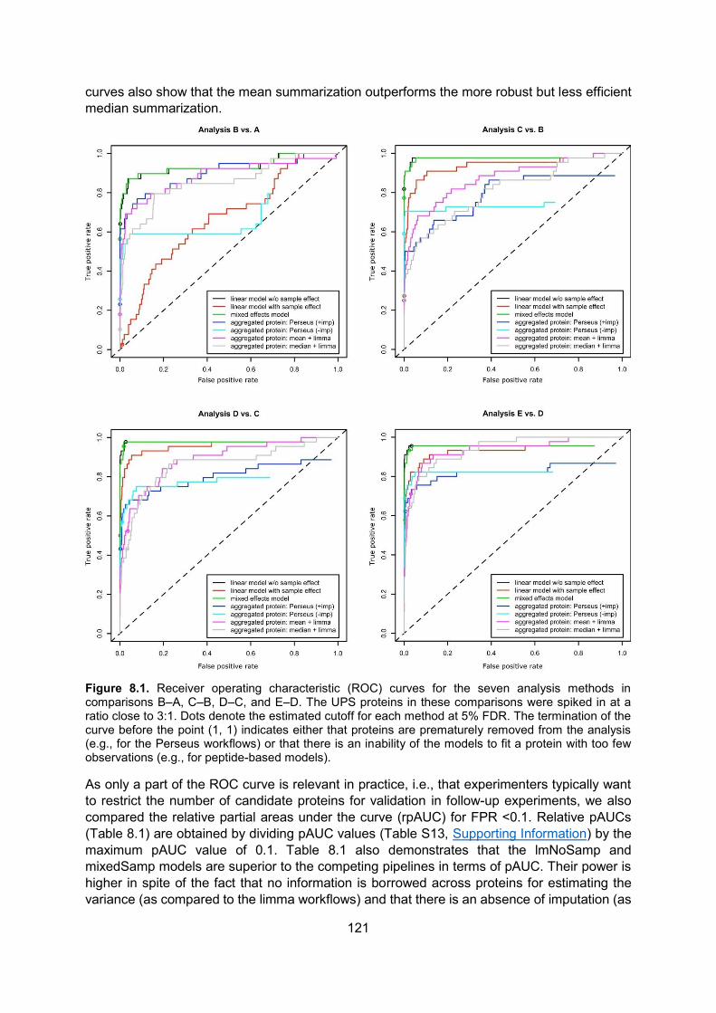
121

curves also show that the mean summarization outperforms the more robust but less efficient median summarization.

Figure 8.1. Receiver operating characteristic (ROC) curves for the seven analysis methods in comparisons B–A, C–B, D–C, and E–D. The UPS proteins in these comparisons were spiked in at a ratio close to 3:1. Dots denote the estimated cutoff for each method at 5% FDR. The termination of the curve before the point (1, 1) indicates either that proteins are prematurely removed from the analysis (e.g., for the Perseus workflows) or that there is an inability of the models to fit a protein with too few observations (e.g., for peptide-based models).

As only a part of the ROC curve is relevant in practice, i.e., that experimenters typically want to restrict the number of candidate proteins for validation in follow-up experiments, we also compared the relative partial areas under the curve (rpAUC) for FPR <0.1. Relative pAUCs (Table 8.1) are obtained by dividing pAUC values (Table S13, Supporting Information) by the maximum pAUC value of 0.1. Table 8.1 also demonstrates that the lmNoSamp and mixedSamp models are superior to the competing pipelines in terms of pAUC. Their power is higher in spite of the fact that no information is borrowed across proteins for estimating the variance (as compared to the limma workflows) and that there is an absence of imputation (as


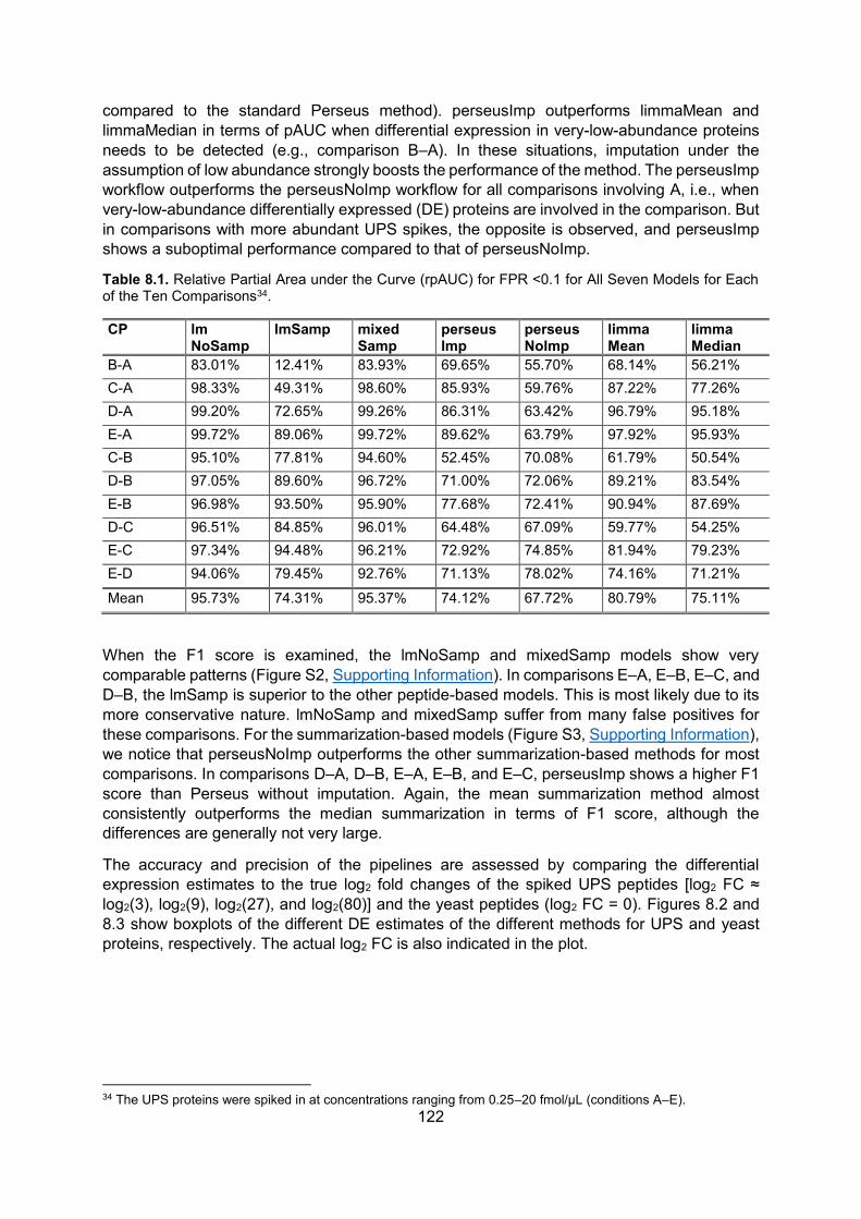
122

compared to the standard Perseus method). perseusImp outperforms limmaMean and limmaMedian in terms of pAUC when differential expression in very-low-abundance proteins needs to be detected (e.g., comparison B–A). In these situations, imputation under the assumption of low abundance strongly boosts the performance of the method. The perseusImp workflow outperforms the perseusNoImp workflow for all comparisons involving A, i.e., when very-low-abundance differentially expressed (DE) proteins are involved in the comparison. But in comparisons with more abundant UPS spikes, the opposite is observed, and perseusImp shows a suboptimal performance compared to that of perseusNoImp.

Table 8.1. Relative Partial Area under the Curve (rpAUC) for FPR <0.1 for All Seven Models for Each of the Ten Comparisons34.

CP lm NoSamp

lmSamp mixed Samp

perseus Imp

perseus NoImp

limma Mean

limma Median

B-A 83.01% 12.41% 83.93% 69.65% 55.70% 68.14% 56.21% C-A 98.33% 49.31% 98.60% 85.93% 59.76% 87.22% 77.26% D-A 99.20% 72.65% 99.26% 86.31% 63.42% 96.79% 95.18% E-A 99.72% 89.06% 99.72% 89.62% 63.79% 97.92% 95.93% C-B 95.10% 77.81% 94.60% 52.45% 70.08% 61.79% 50.54% D-B 97.05% 89.60% 96.72% 71.00% 72.06% 89.21% 83.54% E-B 96.98% 93.50% 95.90% 77.68% 72.41% 90.94% 87.69% D-C 96.51% 84.85% 96.01% 64.48% 67.09% 59.77% 54.25% E-C 97.34% 94.48% 96.21% 72.92% 74.85% 81.94% 79.23% E-D 94.06% 79.45% 92.76% 71.13% 78.02% 74.16% 71.21%

Mean 95.73% 74.31% 95.37% 74.12% 67.72% 80.79% 75.11%

When the F1 score is examined, the lmNoSamp and mixedSamp models show very comparable patterns (Figure S2, Supporting Information). In comparisons E–A, E–B, E–C, and D–B, the lmSamp is superior to the other peptide-based models. This is most likely due to its more conservative nature. lmNoSamp and mixedSamp suffer from many false positives for these comparisons. For the summarization-based models (Figure S3, Supporting Information), we notice that perseusNoImp outperforms the other summarization-based methods for most comparisons. In comparisons D–A, D–B, E–A, E–B, and E–C, perseusImp shows a higher F1 score than Perseus without imputation. Again, the mean summarization method almost consistently outperforms the median summarization in terms of F1 score, although the differences are generally not very large.

The accuracy and precision of the pipelines are assessed by comparing the differential expression estimates to the true log2 fold changes of the spiked UPS peptides [log2 FC ≈ log2(3), log2(9), log2(27), and log2(80)] and the yeast peptides (log2 FC = 0). Figures 8.2 and 8.3 show boxplots of the different DE estimates of the different methods for UPS and yeast proteins, respectively. The actual log2 FC is also indicated in the plot.

34 The UPS proteins were spiked in at concentrations ranging from 0.25–20 fmol/μL (conditions A–E).



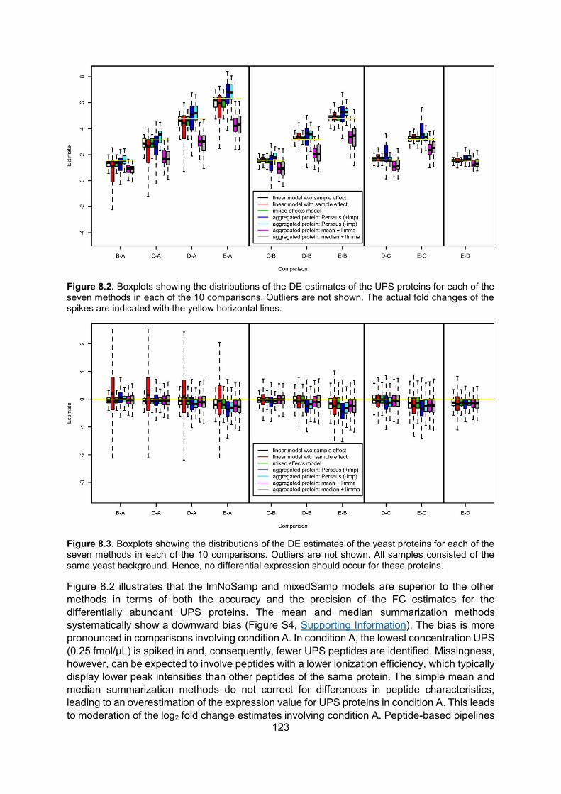
123

Figure 8.2. Boxplots showing the distributions of the DE estimates of the UPS proteins for each of the seven methods in each of the 10 comparisons. Outliers are not shown. The actual fold changes of the spikes are indicated with the yellow horizontal lines.

Figure 8.3. Boxplots showing the distributions of the DE estimates of the yeast proteins for each of the seven methods in each of the 10 comparisons. Outliers are not shown. All samples consisted of the same yeast background. Hence, no differential expression should occur for these proteins.

Figure 8.2 illustrates that the lmNoSamp and mixedSamp models are superior to the other methods in terms of both the accuracy and the precision of the FC estimates for the differentially abundant UPS proteins. The mean and median summarization methods systematically show a downward bias (Figure S4, Supporting Information). The bias is more pronounced in comparisons involving condition A. In condition A, the lowest concentration UPS (0.25 fmol/μL) is spiked in and, consequently, fewer UPS peptides are identified. Missingness, however, can be expected to involve peptides with a lower ionization efficiency, which typically display lower peak intensities than other peptides of the same protein. The simple mean and median summarization methods do not correct for differences in peptide characteristics, leading to an overestimation of the expression value for UPS proteins in condition A. This leads to moderation of the log2 fold change estimates involving condition A. Peptide-based pipelines


124

correcting for peptide effects also suffer from a slight negative bias in comparisons that involve condition A. Note that imputation has a severe impact on the precision. Figure S7 in the Supporting Information also shows that summarization-based limmaMean and limmaMedian methods give the highest root mean squared error (RMSE = [bias2/variance]1/2) among all methods that were evaluated.

Figure 8.3 confirms that the lmNoSamp and the mixedSamp models are favorable in terms of accuracy and precision. For the yeast proteins (non-DE), the median and mean summarization methods show a bias similar to that of competing methods. An increasing downward bias of the log2 FC estimates can be observed for the null proteins (yeast) in comparisons involving increasing UPS concentrations. This becomes very apparent for comparisons that involve condition E. In this condition, a very high fraction of the total protein mass in the sample consists of UPS proteins. Hence, yeast peptides are likely to be masked by UPS, leading to an underestimation of the abundance of yeast peptides in the D and E mix. Most false positive yeast proteins had negative log2 FC estimates as opposed to the spiked UPS proteins, which show positive log2 FC estimates in each comparison. Therefore, issues involving the FDR are likely to be linked to the extreme sample composition under conditions D and E, which invokes an MS bias.(10) The F1 score masks this artifact, as it combines PPV and sensitivity. The same trend is also visible in MA plots for the linear model without sample effect (Figures S10 and S11, Supporting Information). In these graphs, the average FC is plotted in function of the average protein expression for a particular comparison. These graphs are therefore very helpful for screening for artifacts induced by the technical and data analysis workflows. Figure 8.3 also illustrates that the precision reduces with increasing FC, i.e., for comparisons involving conditions D and E. Finally, the lmSamp method shows a dramatic decrease in precision for comparison B–A. This is a data analysis artifact; the model is overidentified for many proteins, leading to the aliasing of sample and treatment effects. Due to the specific model parametrization, the overidentification has a larger impact on comparisons involving condition A.

We also investigated alternative data analysis strategies to alleviate this problem. For the peptide-based lmNoSamp method, we assessed the impact of testing against the median log2 FC of all proteins instead of testing against 0. This slightly improves the observed FDR except for comparisons C–A and D–B and improves the rpAUC except for comparisons D–A, D–B, D–C, and E–C (Table S14, Supporting Information). However, the method still returns too many false positives for the comparisons involving high concentrations (Table S9, Supporting Information). For the summarization-based methods, we assessed the impact of switching the order of the normalization and summarization steps. When the quantile normalization is performed after summarization, the observed FDR improved for comparisons involving D and E, but the performance decreased dramatically for comparisons B–A and C–A (Tables S10–S12. Supporting Information). The ROC curves also suggest that switching the order of the normalization and summarization steps deteriorates the performance of the limmaMean and limmaMedian workflows (Figure S12, Supporting Information).

8.6. Discussion

Our analysis showed that peptide-based models perspicuously outperform summarization-based methods. Both the linear model without sample effect and the mixed model outperform the other methods in terms of accuracy, precision, sensitivity, and specificity. The ROC curves clearly indicate that these methods produce a more reliable ordering of DE proteins than the competing methods. The linear model with sample effect has a suboptimal performance but still outperforms the other methods in comparisons that do not involve A. Due to selective and periodic sampling in both MS stages, not all peptides are being observed or identified in all


javascript:void(0);







125

samples. Moreover, intensities from different peptides of the same protein vary considerably due to differences in cleavage and ionization efficiency among others.(26, 27) Summarization thus typically involves different peptides and a different number of peptides in each sample. This leads to protein expression values with distinct characteristics, which induces bias and incorrect precision of the fold change estimates.

Peptide-based models are superior in correcting for individual peptide effects, which are typically quite strong(18, 19) and accounting for the different number of peptides in each sample. Thus, bias is reduced and improved precision estimates are provided, leading to higher sensitivity and specificity. The mixed model can also account for the correlation that is present in peptides from the same protein within a sample. The peptide-based models with a fixed sample effect suffer from the unstable estimation of fold changes and variance components due to the overfitting of sparse proteins identified by a few peptides. Moreover, the inclusion of a fixed sample effect eliminates the between-sample variability from the analysis. Inference between the samples will be based on an underestimated variance, leading to a higher number of false positives in a top list. In the linear model without sample effect, fewer parameters have to be estimated, and the variances within and between samples are combined in the error term. Hence, the method is less prone to overfitting and incorporates both within- and between-sample variability in the test statistics, leading to a better control of the number of false positives. However, the method does not account for the correlation between peptides from a particular protein within a sample. The mixed modeling approach with a random sample effect does incorporate within- and between-sample variances as well as the within-sample correlation between peptides of the same protein. The mixed model and the linear model without sample effect are more or less on par in terms of all assessed performance criteria. Hence, the increased computational complexity of the mixed model cannot be justified for this particular application. However, in real experiments, more correlation can be expected due to the additional biological variation among samples.

We also showed that the use of FDR thresholds might be flawed under certain experimental conditions. This was observed for comparisons involving conditions D and E, i.e., the samples with the highest spiked-in UPS concentrations. Under these conditions, the UPS proteins correspond to a considerable fraction of the total protein mass in the sample. The ROC curves show that peptide-based methods still produce reliable top lists with a superb ordering, but the use of a 5% FDR threshold was too liberal. Hence, long protein lists are produced with many false positives. The majority of these false positives, however, had FC estimates in the opposite direction as those of spiked UPS proteins. This was due to a systematic downward bias in the FC estimates of nondifferentially expressed yeast proteins. Competitive ionization makes the identification and quantification of yeast peptides cumbersome in samples with highly concentrated UPS spikes. Thus, the majority of false positives originate from technological artifacts rather than from flaws in the data analysis pipeline. We therefore recommend that researchers who are planning to use internal controls in their MS experiments avoid overspiking, as this can have detrimental effects on the quantification of the proteins of interest. Moreover, artifacts similar to those from spiked UPS proteins are bound to occur in certain experimental setups (e.g., undepleted blood plasma proteomic samples are known to be dominated by a few highly abundant proteins, and undepleted green tissue samples from plants will suffer from the omnipresence of RuBisCo). Our analysis showed that experimenters should interpret proteins further down the DE list with care. We therefore advise data analysts to use diagnostic plots based on all fold change estimates for assessing the quality of the FC estimates and for detecting potential artifacts. MA plots and boxplots were shown to be well suited for evaluating candidate DE proteins, to flag critical experimental conditions as well as flaws in the data analysis pipeline.

javascript:void(0);

javascript:void(0);

126

The myriad missing values in quantitative proteomic experiments present severe challenges to the data analysis. The standard MaxQuant pipeline therefore utilizes the match-between runs option to boost the number of peptide intensities that different samples have in common. Moreover, Perseus also incorporates imputation-based routines to deal with missing protein expression values. We showed that imputation is beneficial for detecting differentially expressed proteins with low abundance but performs suboptimally for moderately to highly abundant proteins. Perseus’ standard imputation algorithm assumes that missing values originate from lower intensity values. Hence, the imputation can lead to a downward bias for more abundant proteins. Moreover, experimenters should also be aware that imputation comes at the cost of a decreased precision for the FC estimates.

In general, the current peptide-based methods are prone to overfitting and rely on protein-by-protein variance estimates. Hence, the development of robust methods that can borrow information across peptides and proteins would enable proteomics researchers to further deploy label-free quantitative proteomics.

In summary, we have shown that issues inherent to the methodology create challenges in quantitative proteomics, even in highly controlled and standardized samples such as the CPTAC ones. We then go on to show that downstream statistical data analysis approaches differ in their ability to cope with these different issues, and that the importance of these issues depends on the characteristics of the sample under study (e.g., the dominance of a few highly abundant proteins or large protein concentration ratio differences between two samples). Crucial, perhaps, is the fact that although peptide-based approaches fare better than summarization methods, no single method currently exists that can easily tackle all possible issues in quantitative proteomics data. Hence, more sophisticated data processing approaches that recognize these various issues are needed and can compensate for such issues more successfully across the board.

8.7. Conclusion

In this paper, we compared the performance of peptide-based linear models, mean and median summarization followed by limma analysis, and the standard MaxQuant/Perseus workflow for assessing differential abundance in label-free quantitative proteomics experiments. The evaluation of the performance was assessed using the CPTAC benchmark data set. Peptide-based models outperformed the competing data analysis pipelines in terms of sensitivity, specificity, accuracy, and precision. Modeling quantitative proteomics data at the peptide level allows for the correction of strong peptide-specific effects, which avoids the bias associated with summarization-based methods that aggregate different types of peptide intensities into a single value. Moreover, peptide-based models also improve the precision estimates by accounting for the different numbers of peptides that are identified in a sample. We have also shown that the FDR cutoffs used to determine the length of lists with significant differentially expressed (DE) proteins could become problematic in experimental setups with samples that are dominated by a few very abundant proteins. Technological artifacts might induce bias in the non-DE proteins, which can inflate the number of false positives that are returned at a particular FDR level. However, the ordering of the top DE proteins in the lists was shown to remain valid. We therefore advise proteomics researchers to be careful when spiking internal controls, to deplete the highly abundant proteins, and to use diagnostic plots for assessing the candidate DE proteins as well as the overall quality of the obtained fold change estimates. Finally, standard proteomics software provides experimenters with the ability to impute missing values. Perseus’ imputation strategy was shown to be beneficial for detecting DE proteins with low abundance but at the cost of reduced precision as well as a suboptimal performance for

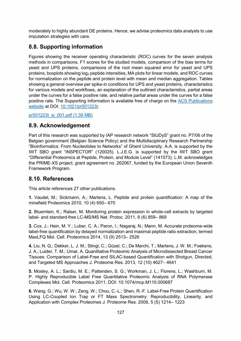
127

moderately to highly abundant DE proteins. Hence, we advise proteomics data analysts to use imputation strategies with care.

8.8. Supporting information

Figures showing the receiver operating characteristic (ROC) curves for the seven analysis methods in comparisons, F1 scores for the studied models, comparison of the bias terms for yeast and UPS proteins, comparisons of the root mean squared error for yeast and UPS proteins, boxplots showing log2 peptide intensities, MA plots for linear models, and ROC curves for normalization on the peptide and protein level with mean and median aggregation. Tables showing a general overview per spike-in conditions for UPS and yeast proteins, characteristics for various models and workflows, an explanation of the outlined characteristics, partial areas under the curves for a false positive rate, and relative partial areas under the curves for a false positive rate. The Supporting Information is available free of charge on the ACS Publications website at DOI: 10.1021/pr501223t.

pr501223t_si_001.pdf (1.38 MB)

8.9. Acknowledgement Part of this research was supported by IAP research network “StUDyS” grant no. P7/06 of the Belgian government (Belgian Science Policy) and the Multidisciplinary Research Partnership “Bioinformatics: From Nucleotides to Networks” of Ghent University. A.A. is supported by the IWT SBO grant “INSPECTOR” (120025). L.J.E.G. is supported by the IWT SBO grant “Differential Proteomics at Peptide, Protein, and Module Level” (141573). L.M. acknowledges the PRIME-XS project, grant agreement no. 262067, funded by the European Union Seventh Framework Program.

8.10. References This article references 27 other publications.

1. Vaudel, M.; Sickmann, A.; Martens, L. Peptide and protein quantification: A map of the minefield Proteomics 2010, 10 (4) 650– 670

2. Bluemlein, K.; Ralser, M. Monitoring protein expression in whole-cell extracts by targeted label- and standard-free LC-MS/MS Nat. Protoc. 2011, 6 (6) 859– 869

3. Cox, J.; Hein, M. Y.; Luber, C. A.; Paron, I.; Nagaraj, N.; Mann, M. Accurate proteome-wide label-free quantification by delayed normalization and maximal peptide ratio extraction, termed MaxLFQ Mol. Cell. Proteomics 2014, 13 (9) 2513– 2526

4. Liu, N. Q.; Dekker, L. J. M.; Stingl, C.; Güzel, C.; De Marchi, T.; Martens, J. W. M.; Foekens, J. A.; Luider, T. M.; Umar, A. Quantitative Proteomic Analysis of Microdissected Breast Cancer Tissues: Comparison of Label-Free and SILAC-based Quantification with Shotgun, Directed, and Targeted MS Approaches J. Proteome Res. 2013, 12 (10) 4627– 4641

5. Mosley, A. L.; Sardiu, M. E.; Pattenden, S. G.; Workman, J. L.; Florens, L.; Washburn, M. P. Highly Reproducible Label Free Quantitative Proteomic Analysis of RNA Polymerase Complexes Mol. Cell. Proteomics 2011, DOI: 10.1074/mcp.M110.000687

6. Wang, G.; Wu, W. W.; Zeng, W.; Chou, C.-L.; Shen, R.-F. Label-Free Protein Quantification Using LC-Coupled Ion Trap or FT Mass Spectrometry: Reproducibility, Linearity, and Application with Complex Proteomes J. Proteome Res. 2006, 5 (5) 1214– 1223

http://pubs.acs.org/

http://pubs.acs.org/

http://pubs.acs.org/doi/abs/10.1021/pr501223t

https://pubs.acs.org/doi/suppl/10.1021/pr501223t/suppl_file/pr501223t_si_001.pdf

128

7. Silva, J. C.; Gorenstein, M. V.; Li, G.-Z.; Vissers, J. P. C.; Geromanos, S. J. Absolute Quantification of Proteins by LCMSE: A Virtue of Parallel ms Acquisition Mol. Cell. Proteomics 2006, 5 (1) 144– 156

8. Vaudel, M.; Sickmann, A.; Martens, L. Current methods for global proteome identification Expert Rev. Proteomics 2012, 9 (5) 519– 532

9. Peng, M.; Taouatas, N.; Cappadona, S.; van Breukelen, B.; Mohammed, S.; Scholten, A.; Heck, A. J. R. Protease bias in absolute protein quantitation Nat. Methods 2012, 9 (6) 524– 525

10. Schliekelman, P.; Liu, S. Quantifying the Effect of Competition for Detection between Coeluting Peptides on Detection Probabilities in Mass-Spectrometry-Based Proteomics J. Proteome Res. 2013, 13 (2) 348– 361

11. Kumar, C.; Mann, M. Bioinformatics analysis of mass spectrometry-based proteomics data sets FEBS Lett. 2009, 583 (11) 1703– 1712

12. Liu, H.; Sadygov, R. G.; Yates, J. R. A Model for Random Sampling and Estimation of Relative Protein Abundance in Shotgun Proteomics Anal. Chem. 2004, 76 (14) 4193– 4201

13. Bantscheff, M.; Schirle, M.; Sweetman, G.; Rick, J.; Kuster, B. Quantitative mass spectrometry in proteomics: a critical review Anal. Bioanal. Chem. 2007, 389 (4) 1017– 31

14. Mueller, L. N.; Brusniak, M.-Y.; Mani, D. R.; Aebersold, R. An Assessment of Software Solutions for the Analysis of Mass Spectrometry Based Quantitative Proteomics Data J. Proteome Res. 2008, 7 (1) 51– 61

15. Old, W. M.; Meyer-Arendt, K.; Aveline-Wolf, L.; Pierce, K. G.; Mendoza, A.; Sevinsky, J. R.; Resing, K. A.; Ahn, N. G. Comparison of Label-free Methods for Quantifying Human Proteins by Shotgun Proteomics Mol. Cell. Proteomics 2005, 4 (10) 1487– 1502

16. Théron, L.; Gueugneau, M.; Coudy, C.; Viala, D.; Bijlsma, A.; Butler-Browne, G.; Maier, A.; Béchet, D.; Chambon, C. Label-free Quantitative Protein Profiling of vastus lateralis Muscle During Human Aging Mol. Cell. Proteomics 2014, 13 (1) 283– 294

17. Hubner, N. C.; Bird, A. W.; Cox, J.; Splettstoesser, B.; Bandilla, P.; Poser, I.; Hyman, A.; Mann, M. Quantitative proteomics combined with BAC TransgeneOmics reveals in vivo protein interactions J. Cell Biol. 2010, 189 (4) 739– 754

18. Clough, T.; Key, M.; Ott, I.; Ragg, S.; Schadow, G.; Vitek, O. Protein Quantification in Label-Free LC-MS Experiments J. Proteome Res. 2009, 8 (11) 5275– 5284

19. Karpievitch, Y.; Stanley, J.; Taverner, T.; Huang, J.; Adkins, J. N.; Ansong, C.; Heffron, F.; Metz, T. O.; Qian, W.-J.; Yoon, H.; Smith, R. D.; Dabney, A. R. A statistical framework for protein quantitation in bottom-up MS-based proteomics Bioinformatics 2009, 25 (16) 2028– 2034

20. Paulovich, A. G.; Billheimer, D.; Ham, A.-J. L.; Vega-Montoto, L.; Rudnick, P. A.; Tabb, D. L.; Wang, P.; Blackman, R. K.; Bunk, D. M.; Cardasis, H. L.; Clauser, K. R.; Kinsinger, C. R.; Schilling, B.; Tegeler, T. J.; Variyath, A. M.; Wang, M.; Whiteaker, J. R.; Zimmerman, L. J.; Fenyo, D.; Carr, S. A.; Fisher, S. J.; Gibson, B. W.; Mesri, M.; Neubert, T. A.; Regnier, F. E.; Rodriguez, H.; Spiegelman, C.; Stein, S. E.; Tempst, P.; Liebler, D. C. Interlaboratory Study Characterizing a Yeast Performance Standard for Benchmarking LC-MS Platform Performance Mol. Cell. Proteomics 2010, 9 (2) 242– 254

129

21. Cox, J.; Hein, M. Y.; Luber, C. A.; Paron, I.; Nagaraj, N.; Mann, M. Accurate Proteome-wide Label-free Quantification by Delayed Normalization and Maximal Peptide Ratio Extraction, Termed MaxLFQ Mol. Cell. Proteomics 2014, 13 (9) 2513– 2526

22. Cox, J.; Mann, M. MaxQuant enables high peptide identification rates, individualized p.p.b.-range mass accuracies and proteome-wide protein quantification Nat. Biotechnol. 2008, 26 (12) 1367– 1372

23. Benjamini, Y.; Hochberg, Y. Controlling the False Discovery Rate: A Practical and Powerful Approach to Multiple Testing J. R. Stat. Soc.: Series B 1995, 57 (1) 289– 300

24. Smyth, G. K., Linear models and empirical bayes methods for assessing differential expression in microarray experiments. Stat Appl. Genet. Mol. Biol. 2004, 3, Article 3.

25. Satterthwaite, F. E. An approximate distribution of estimates of variance components Biometrics 1946, 2 (6) 110– 4

26. Rodriguez, J.; Gupta, N.; Smith, R. D.; Pevzner, P. A. Does Trypsin Cut Before Proline? J. Proteome Res. 2008, 7 (1) 300– 305

27. Abaye, D. A.; Pullen, F. S.; Nielsen, B. V. Peptide polarity and the position of arginine as sources of selectivity during positive electrospray ionisation mass spectrometry Rapid Commun. Mass Spectrom. 2011, 25 (23) 3597– 3608

131

9. ROBUST QUANTIFICATION FOR LABEL-FREE MASS SPECTROMETRY-BASED PROTEOMICS

Chapter 9 describes MSqRob, our R software package for improved differential protein abundance analysis in label-free MS-based proteomics. MSqRob is freely available on GitHub (https://github.com/statOmics/MSqRob) and is implemented in a "Shiny" user-friendly graphical interface.

In section 9.1, I introduce MSqRob as a new algorithm for the analysis of quantitative proteomics data that improves protein quantification by combining three innovative statistical approaches: ridge regression, empirical Bayes variance estimation, and M-estimation with Huber weights. MSqRob is both more precise and more accurate than state-of-the-art tools. I developed and implemented MSqRob as an R package and wrote the manuscript together with my supervisors.

Section 9.2 is published as an invited tutorial paper in which I outline key statistical concepts to help researchers to design proteomics experiments and showcases of quantitative proteomics data analysis with MSqRob. For this manuscript, I designed and performed analyses, set up the GitHub repository and wrote the paper together with my supervisors.

9.1. Peptide-level Robust Ridge Regression Improves Estimation, Sensitivity, and Specificity in Data-dependent Quantitative Label-free Shotgun Proteomics Goeminne L.J.E., Gevaert K. and Clement L. (2016). Peptide-level Robust Ridge Regression Improves Estimation, Sensitivity, and Specificity in Data-dependent Quantitative Label-free Shotgun Proteomics. Molecular & Cellular Proteomics. 15(2), 657-668 9.1.1. Associated data

Supplementary Materials

Supplemental Data

supp_15_2_657__index.html (2.4K)

GUID: 9B15C066-3091-4E71-980A-55F4B6EE0B27

10.1074_M115.055897_mcp.M115.055897-1.pdf (7.0M)

GUID: 401B1F9E-2C1B-4FA6-9374-9048987008F2

10.1074_M115.055897_mcp.M115.055897-2.xlsx (208K)

GUID: B2490BE1-84E1-49D7-8951-5CB1D9597D83

10.1074_M115.055897_mcp.M115.055897-3.zip (72M)

GUID: 6BF2E185-A0C2-4F19-B71D-5999CF7F6AF2

https://github.com/statOmics/MSqRob

https://www.ncbi.nlm.nih.gov/pmc/articles/PMC4739679/

https://www.ncbi.nlm.nih.gov/pmc/articles/PMC4739679/bin/supp_15_2_657__index.html

https://www.ncbi.nlm.nih.gov/pmc/articles/PMC4739679/bin/10.1074_M115.055897_mcp.M115.055897-1.pdf

https://www.ncbi.nlm.nih.gov/pmc/articles/PMC4739679/bin/10.1074_M115.055897_mcp.M115.055897-2.xlsx

https://www.ncbi.nlm.nih.gov/pmc/articles/PMC4739679/bin/10.1074_M115.055897_mcp.M115.055897-3.zip

132

9.1.2. Abstract

Peptide intensities from mass spectra are increasingly used for relative quantitation of proteins in complex samples. However, numerous issues inherent to the mass spectrometry workflow turn quantitative proteomic data analysis into a crucial challenge. We and others have shown that modeling at the peptide level outperforms classical summarization-based approaches, which typically also discard a lot of proteins at the data preprocessing step. Peptide-based linear regression models, however, still suffer from unbalanced datasets due to missing peptide intensities, outlying peptide intensities and overfitting. Here, we further improve upon peptide-based models by three modular extensions: ridge regression, improved variance estimation by borrowing information across proteins with empirical Bayes and M-estimation with Huber weights. We illustrate our method on the CPTAC spike-in study and on a study comparing wild-type and ArgP knock-out Francisella tularensis proteomes. We show that the fold change estimates of our robust approach are more precise and more accurate than those from state-of-the-art summarization-based methods and peptide-based regression models, which leads to an improved sensitivity and specificity. We also demonstrate that ionization competition effects come already into play at very low spike-in concentrations and confirm that analyses with peptide-based regression methods on peptide intensity values aggregated by charge state and modification status (e.g. MaxQuant's peptides.txt file) are slightly superior to analyses on raw peptide intensity values (e.g. MaxQuant's evidence.txt file).

9.1.3. Introduction

High-throughput LC-MS-based proteomic workflows are widely used to quantify differential protein abundance between samples. Relative protein quantification can be achieved by stable isotope labeling workflows such as metabolic (1, 2) and postmetabolic labeling (3–6). These types of experiments generally avoid run-to-run differences in the measured peptide (and thus protein) content by pooling and analyzing differentially labeled samples in a single run. Label-free quantitative (LFQ)1 workflows become increasingly popular as the often expensive and time-consuming labeling protocols are omitted. Moreover, LFQ proteomics allows for more flexibility in comparing samples and tends to cover a larger area of the proteome at a higher dynamic range (7, 8). Nevertheless, the nature of the LFQ protocol makes shotgun proteomic data analysis a challenging task. Missing values are omnipresent in proteomic data generated by data-dependent acquisition workflows, for instance because of low-abundant peptides that are not always fragmented in complex peptide mixtures and a limited number of modifications and mutations that can be accounted for in the feature search. Moreover, the overall abundance of a peptide is determined by the surroundings of its corresponding cleavage sites as these influence protease cleavage efficiency (9). Similarly, some peptides are more easily ionized than others (10). These issues not only lead to missing peptides, but also increase variability in individual peptide intensities. The discrete nature of MS1 sampling following continuous elution of peptides from the LC column leads to increased variability in peptide quantifications. Finally, competition for ionization and co-elution of other peptides with similar m/z values may cause biased quantifications (11). However, note that in this respect, using data-independent acquisition (DIA), all peptide ions (or all peptide ions within a certain m/z range, depending on the method used) are fragmented simultaneously, resulting in multiplexed MS/MS spectra (12, 13). Hence, issues of missing fragment spectra are less a problem with DIA, however, some of its challenges lie in deconvoluting MS/MS spectra and mapping their features to their corresponding peptides (14).

Standard data analysis pipelines for DDA-LFQ proteomics can be divided into two groups: spectral counting techniques, which are based on counting the number of peptide features as

https://www.ncbi.nlm.nih.gov/pmc/articles/PMC4739679/#B1




https://www.ncbi.nlm.nih.gov/pmc/articles/PMC4739679/#G1









133

a proxy for protein abundance (15), and intensity-based methods that quantify peptide features by measuring their corresponding spectral intensities or areas under the peaks in either MS or MS/MS spectra. Spectral counting is intuitive and easy to perform, but, the determination of differences in peptide and thus protein levels is not as precise as intensity-based methods, especially when analyzing rather small differences (16). More fundamentally, spectral counting ignores a large part of the information that is available in high-precision mass spectra. Further, dynamic exclusion during LC-MS/MS analysis, meant to increase the overall number of peptides that are analyzed, can worsen the linear dynamic range of these methods (17). Also, any changes in the MS/MS sampling conditions will prevent comparisons between runs. Intensity-based methods are more sensitive than spectral counting (18). Among intensity-based methods, quantification on the MS-level is somewhat more accurate than summarizing the MS/MS-level feature intensities (19). Therefore, we further focus on improving data analysis methods for MS-level quantification.

Typical intensity-based workflows summarize peptide intensities to protein intensities before assessing differences in protein abundances (20). Peptide-based linear regression models estimate protein fold changes directly from peptide intensities and outperform summarization-based methods by reducing bias and generating more correct precision estimates (21, 22). However, peptide-based linear regression models suffer from overfitting due to extreme observations and the unbalanced nature of proteomics data; i.e. different peptides and a different number of peptides are typically identified in each sample. We illustrate this using the CPTAC spike-in data set where 48 human UPS1 proteins were spiked at five different concentrations in a 60 ng protein/μl yeast lysate. Thus, when comparing different spike-in concentrations, only the human proteins should be flagged as differentially abundant (DA), whereas the yeast proteins should not be flagged as DA (null proteins). Fig. 9.1 illustrates the structure of missing data in label-free shotgun proteomics experiments using a representative DA UPS1 protein from the CPTAC spike-in study: missing peptides in the lowest spike-in condition tend to have rather low log2 intensity values in higher spike-in conditions compared to peptides that were not missing in both conditions, which supports the fact that the missing value problem in label-free shotgun proteomic data is largely intensity-dependent (23).

Figure 9.1. Missing peptides are often low abundant. The boxplots show the log2 intensity distributions for each of the 33 identified peptides corresponding to the human UPS1 protein cytoplasmic Histidyl-tRNA synthetase (P12081) from the CPTAC dataset in conditions 6A (spike-in concentration










https://www.ncbi.nlm.nih.gov/protein/P12081

134

0.25 fmol UPS1 protein/μl) and 6B (spike-in concentration 0.74 fmol UPS1 protein/μl). Vertical dotted lines indicate peptides present in both conditions. Note, that most peptides that were not detected in condition 6A exhibit low log2 intensity values in condition 6B (colored in red).

Fig. 9.2 shows the quantile normalized log2 intensity values for the peptides corresponding to the yeast null protein CG121 together with average log2 intensity estimates for each condition based on protein-level MaxLFQ intensities, as well as estimates derived from a peptide-based linear model. Here, three important remarks can be made:

(1) CG121 is a yeast background protein, for which the true concentration is thus equal in all conditions, which appears to be monitored as such by MaxLFQ, except in conditions 6B and 6E (for the latter, no estimate is available). The LM estimate, however, is more reliable but seems to suffer from overfitting.

(2) A lot of shotgun proteomic datasets are very sparse, causing a large sample-to-sample variability. Constructing a linear model based on a limited number of observations will thus lead to unstable variance estimates. Intuitively, a small sample drawn from a given population might “accidentally” show a very small variance while another small sample from the same population might display a very large variance just by random chance. This effect is clear from the sizes of the boxes. The interquartile range is twice as large in condition 6E compared to condition 6C. This issue leads to false positives since some proteins with very few observations are flagged as DA with very high statistical evidence solely due to their low observed variance (24).

(3) Two observed features at log2 intensities 14.0 and 14.3 in condition 6B have a strong influence on the parameter estimate for this condition. Without these extreme observations, the 6B estimate lies closer to the estimates in the other conditions. As missingness is strongly intensity-dependent, these low intensity values could easily become missing values in subsequent experiments. More generally, a strong influence of only one or two peptides on the average protein level intensity estimate for a condition is an unfavorable property.


135

Figure 9.2. Effect of outliers, variability, and sparsity of peptide intensities on abundance estimations. The figure shows log2 transformed quantile normalized peptide intensities for the yeast null protein CG121 from the CPTAC data set for spike-in conditions 6A, 6B, 6C, 6D, and 6E. Each color denotes a different condition. Connected crosses: average protein log2 intensity estimates for each condition are provided for a traditional protein level workflow where the mean of the protein-level MaxLFQ values was calculated (MaxLFQ, blue), the estimates of the peptide-based regression model fitted with ordinary least squares (LM, black) and the estimates of the peptide based ordinary least squares fit after omitting the two lowest observations in condition 6B (LM-extremes, orange). In condition 6E there were not enough data points to provide a MaxLFQ protein-level estimate. Boxes denote the interquartile range (IQR) of the log2 transformed quantile normalized peptide intensities in each condition with the median indicated as a thick horizontal line inside each box. Whiskers extend to the most extreme data point that lies no more than 1.5 times the IQR from the box. Points lying beyond the whiskers are generally considered as outliers. Note, that the presence of two low-intensity peptide observations in concentration 6B has a strong effect on the estimates for both MaxLFQ and LM.

These issues illustrate that state-of-the-art analysis methods experience difficulties in coping with peptide imbalances that are inherent to DDA LFQ proteomics data. We here propose three modular improvements to deal with the problems of overfitting, sample-to-sample variability and outliers:

(1) Ridge regression, which penalizes the size of the model parameters. Shrinkage estimators can strongly improve reproducibility and overall performance as they have a lower overall mean squared error compared to ordinary least squares estimators (25–27).

(2) Empirical Bayes variance estimation, which shrinks the individual protein variances toward a common prior variance, hence stabilizing the variance estimation.

(3) M-estimation with Huber weights, which will make the estimators more robust toward outliers (28).

We illustrate our method on the CPTAC Study 6 spike-in data and a published ArgP knock-out Francisella tularensis proteomics experiment and show that our method provides more stable log2 FC estimates and a better DA ranking than competing methods.




136

9.1.4. Experimental procedures

CPTAC Spike-in Data Set

The publicly available Study 6 of the Clinical Proteomic Technology Assessment for Cancer (29) is used to evaluate the performance of our method. Raw data can be accessed at https://cptac-data-portal.georgetown.edu/cptac/public?scope=Phase+I. In this study, the Sigma Universal Protein Standard mixture 1 (UPS1, Sigma-Aldrich, St. Louis, MO) containing 48 different human proteins was spiked into a 60 ng protein/μl Saccharomyces cerevisiae strain BY4741 (MATa, leu2Δ0, met15Δ0, ura3Δ0, his3Δ1) lysate in five different concentrations (6A: 0.25 fmol UPS1 proteins/μl; 6B: 0.74 fmol UPS1 proteins/μl; 6C: 2.22 fmol UPS1 proteins/μl; 6D: 6.67 fmol UPS1 proteins/μl; and 6E: 20 fmol UPS1 proteins/μl). These samples were sent to five independent laboratories and analyzed on seven different instruments. For convenience, we limited ourselves to the data originating from the LTQ-Orbitrap at site 86, LTQ-Orbitrap O at site 65 and LTQ-Orbitrap W at site 56. Samples were run three times on each instrument. The used dataset thus features five different samples, each analyzed in threefold on three different instruments. Raw data files were searched using MaxQuant version 1.5.2.8 (30) with the following settings. As variable modifications we allowed acetylation (protein N terminus), methionine oxidation (to methionine-sulfoxide) and N-terminal glutamine to pyroglutamate conversion. As a fixed modification, we selected carbamidomethylation on cysteine residues as all samples were treated with iodoacetamide. We used the enzymatic rule of trypsin/P with a maximum of 2 missed cleavages and allowed MaxQuant to perform matching between runs with a match time window of 0.7 min and an alignment time window of 20 min. The main search peptide tolerance was set to 4.5 ppm and the ion trap MS/MS match tolerance was set to 0.5 Da. Peptide-to-spectrum match level was set at 1% FDR with an additional minimal Andromeda score of 40 for modified peptides as these settings are most commonly used by researchers. Protein FDR was set at 1% and estimated by using the reversed search sequences. We performed label-free quantitation with MaxQuant's standard settings. The maximal number of modifications per peptide was set to 5. As a search FASTA file we used the 6718 reviewed proteins present in the Saccharomyces cerevisiae (strain ATCC 204508/S288c) proteome downloaded from Uniprot at March 27, 2015 supplemented with the 48 human UPS1 protein sequences. Potential contaminants present in the contaminants.fasta file that comes with MaxQuant were automatically added to the search space by the software. For protein quantification in the proteinGroups.txt file, we used unique and razor peptides and allowed all modifications as all samples originate in essence from the same yeast lysate and the same UPS1 spike-in sample.

Francisella tularensis Data Set

The data of Ramond et al. (31) is used to illustrate our method on a real biological experiment. Both raw and processed data are publicly available and can be found in the PRIDE repository at http://www.ebi.ac.uk/pride/archive/projects/PXD001584. The authors explored changes in the proteome of the facultative intracellular pathogenic coccobacillus Francisella tularensis after gene deletion of a newly identified arginine transporter, ArgP. Both wild-type and ArgP mutants were grown in biological triplicate. Each biological replicate was analyzed in technical triplicate via label-free LC-MS/MS. Data were processed with MaxQuant version 1.4.1.2 and potential contaminants and reverse sequences were removed. In addition, only proteins present with at least two peptides in at least 9 out of the 18 replicates were retained. Subsequent data analysis via t-tests on imputed LFQ intensities was performed.


https://cptac-data-portal.georgetown.edu/cptac/public?scope=Phase+I



http://www.ebi.ac.uk/pride/archive/projects/PXD001584

137

Summarization-based Analysis

MaxLFQ+Perseus

This is a standard summarization-based analysis pipeline that is available in the popular MaxQuant-Persues software package (21). Briefly, the MaxQuant ProteinGroups.txt file was loaded into Perseus version 1.5.1.6, potential contaminants that did not correspond to any UPS1 protein as well as reversed sequences and proteins that were only identified by site (thus only by a peptide carrying a modified residue) were removed from the data set. MaxLFQ intensities (32) were log2 transformed and pairwise comparisons between conditions were done via t-tests.

MaxLFQ+limma

The MaxQuant ProteinGroups.txt file is used as input for R version 3.1.2 (Pumpkin Helmet) (33). Potential contaminants and reversed sequences (see above) were removed from the data set. The MaxLFQ intensities were log2 transformed and analyzed in limma, an R/Bioconductor package for the analysis of microarray and next-generation sequencing data (34). Limma makes use of posterior variance estimators to stabilize the naive variance estimator by borrowing strength across proteins (see also below).

Peptide-based Model Analysis

Data Preprocessing

MaxQuant's peptides.txt file was read into R version 3.1.2, the peptide intensities were log2 transformed and quantile normalized (35, 36). Many other normalization approaches do exist, however, comparing them is beyond the scope of this paper (24, 36–38). Reversed sequences and potential contaminants were removed from the data. For the CPTAC dataset, we only removed potential contaminants that did not map to any UPS1 protein. MaxQuant assigns proteins to protein groups using an Occam's razor approach. However, to avoid the added complexity of proteins mapped to multiple protein groups, we discarded peptides belonging to protein groups that contained one or more proteins that were also present in a smaller protein group. Next, peptides were grouped per protein group in a data frame. Finally, values belonging to peptide sequences that appeared only once were removed as the model parameter for the peptide effect for these sequences is unidentifiable. For notational convenience, a unique protein or protein group is referred to as a protein in the remainder of this article.

Benchmark Peptide-based Model

We start from the peptide-based linear regression models as proposed by Daly et al. (39) Clough et al. (22) and Karpievitch et al. (40), of which we have independently proven their superior performance compared to summarization-based workflows (21). In general, the following model is proposed:

𝑦𝑖𝑗𝑘𝑙𝑚𝑛 = 𝛽𝑖𝑗𝑡𝑟𝑒𝑎𝑡 + 𝛽𝑖𝑘

𝑝𝑒𝑝 + 𝛽𝑖𝑙𝑏𝑖𝑜𝑟𝑒𝑝 + 𝛽𝑖𝑚

𝑡𝑒𝑐ℎ𝑟𝑒𝑝 + 𝜀𝑖𝑗𝑘𝑙𝑚𝑛

(Eq. 1)

with yijklmn the nth log2-transformed normalized feature intensity for the ith protein under the jth treatment (treat), the kth peptide sequence (pep), the lth biological repeat (biorep) and the mth technical repeat (techrep) and εijklmn a normally distributed error term with mean zero and protein specific variance σi

2. The 𝛽's denote the effect sizes for treat, pep, biorep and techrep for the ith protein.














138

Robust Ridge Model

Our novel approach improves the estimation of the model parameters in (Eq. 1) via three extensions: (1) ridge regression, which leads to shrunken yet more stable log2 fold change (FC) estimates, (2) Empirical Bayes estimation of the variance, which further stabilizes variance estimators, and (3) M-estimation with Huber weights, which reduces the impact of outlying peptide intensities. For the robust ridge model, degrees of freedom are calculated using the trace of the hat matrix.

1. Ridge Regression

The ordinary least squares (OLS) estimates for protein i are defined as the parameter estimates that minimize the following loss function:

∑ 𝑒𝑖𝑗𝑘𝑙𝑚𝑛2

𝑗𝑘𝑙𝑚𝑛

= ∑ (𝑦𝑖𝑗𝑘𝑙𝑚𝑛 − 𝛽𝑖𝑗𝑡𝑟𝑒𝑎𝑡 − 𝛽𝑖𝑘

𝑝𝑒𝑝 − 𝛽𝑖𝑙𝑏𝑖𝑜𝑟𝑒𝑝 − 𝛽𝑖𝑚

𝑡𝑒𝑐ℎ𝑟𝑒𝑝)2


(Eq. 2)

With eijklmn the residual errors and Xijklmn the row of the design matrix corresponding to observation yijklmn.

Ridge regression shrinks the regression parameters by imposing a penalty on their magnitude. The ridge regression estimator is obtained by minimizing a penalized least squares loss function:

∑ 𝑒𝑖𝑗𝑘𝑙𝑚𝑛2


+ 𝜆𝑖𝑝𝑒𝑝 ∑𝛽𝑖𝑘

𝑝𝑒𝑝2

𝑘

+ 𝜆𝑖𝑏𝑖𝑜𝑟𝑒𝑝 ∑𝛽𝑖𝑙

𝑏𝑖𝑜𝑟𝑒𝑝2

𝑙

+ 𝜆𝑖𝑡𝑒𝑐ℎ𝑟𝑒𝑝 ∑𝛽𝑖𝑚

𝑡𝑒𝑐ℎ𝑟𝑒𝑝2

𝑚

(Eq. 3)

With each 𝜆 a ridge penalty for the parameter estimator �̂� corresponding to an effect in Eq. 1. When the 𝜆s are larger than zero, the ridge estimators for �̂� will be shrunken toward 0. This introduces some bias but reduces the variability of the parameter estimator, which makes shrinkage estimators theoretically more stable and more accurate (i.e. they tend to have a lower root mean squared error (RMSE) compared to the OLS estimator) (25–27). On the one hand, �̂�'s estimated by only a few observations will experience a strong correction toward 0, protecting against overfitting. On the other hand, �̂�'s that can be estimated based on many observations will exhibit a negligible bias because the ridge penalty will be dominated by the sum of the squared errors, which reflects that these �̂�'s can be estimated more reliably. We choose to tune each 𝜆 separately because the variability on the peptide effect seems generally much larger than the variability on the other effect terms. 𝜆 penalties can be tuned via cross-validation, but in this work, we exploit the link between mixed models and ridge regression (41) and estimate the penalties by implementing ridge regression within the lme4 package (42) in

R. 𝜆𝑡𝑟𝑒𝑎𝑡 then equals �̂�𝑖2

�̂�𝛽𝑡𝑟𝑒𝑎𝑡,𝑖2 with �̂�𝑖 the estimated residual variance and �̂�𝛽𝑡𝑟𝑒𝑎𝑡,𝑖

2 the estimated

variance captured by the treatment effect for peptide intensities from protein i (Chapter 5, 41). The standard errors of the parameter estimators and contrasts of interest are based on the bias-adjusted variance estimator (Chapter 6, 41).

2. Empirical Bayes Variance Estimations

In the introduction we argued that data sparsity can lead to unstable variance estimates. In order to stabilize the residual variance estimation, we shrink the estimated protein specific

https://www.ncbi.nlm.nih.gov/pmc/articles/PMC4739679/#FD1








139

variances toward a pooled estimate over all proteins using an empirical Bayesian approach (43) implemented in the limma R/Bioconductor-package (44). In that way, the information contained in all proteins is borrowed to stabilize the variance estimates of proteins with few observations. Hence, the small variances will increase, while large variances will decrease. This avoids that proteins that exhibit a small FC and a tiny variance will appear highly significantly. Also, the number of degrees of freedom for all these so-called moderated t-tests will increase compared to normal t-tests.

3. M-estimation With Huber Weights

As we have shown in the introduction (see Fig. 9.2), outlying peptides might have a severe impact on the parameter estimates, especially in conditions with few identified features. We therefore propose to adopt M-estimation with Huber weights to diminish the impact of outlying observations. Combining ridge regression with M-estimation leads to the following penalized weighted least squares loss function:

∑ 𝑤𝑖𝑗𝑘𝑙𝑚𝑛𝑒𝑖𝑗𝑘𝑙𝑚𝑛2


+ 𝜆𝑖𝑡𝑟𝑒𝑎𝑡 ∑𝛽𝑖𝑗

𝑡𝑟𝑒𝑎𝑡2

𝑗

+ 𝜆𝑖𝑝𝑒𝑝 ∑𝛽𝑖𝑘

𝑝𝑒𝑝2

𝑘

+ 𝜆𝑖𝑏𝑖𝑜𝑟𝑒𝑝 ∑𝛽𝑖𝑙

𝑏𝑖𝑜𝑟𝑒𝑝2

𝑙

+ 𝜆𝑖𝑡𝑒𝑐ℎ𝑟𝑒𝑝 ∑𝛽𝑖𝑚

𝑡𝑒𝑐ℎ𝑟𝑒𝑝2

𝑚

(Eq. 4)

Herein, wijklmn is a Huber weight that weighs down observations with high residuals.

False Discovery Rate

For both peptide-based models and MaxLFQ+limma, p values are adjusted for multiple testing with the Benjamini-Hochberg FDR procedure (45). Perseus uses a permutation-based FDR that turns out to be very close to the Benjamini-Hochberg procedure. The FDR is controlled at the 5% level in all analyses.

9.1.5. Results

We decided to compare our method to three competing methods using data from the CPTAC spike-in benchmark study. Additionally, its advantages are demonstrated in a case study that was originally analyzed with a standard summarization-based approach. For peptide-based models the use of MaxQuant's peptides.txt file, which contains summed up peptide level data, slightly increased the discriminative power as compared to analyses using the MaxQuant's evidence.txt file, which contains individual intensities for each identified feature (supplemental Fig. S7, File S1). Therefore, all peptide-based models are based on the peptides.txt file.

1. Evaluation Using Data From a Spike-in Benchmark Study

The performances of the different methods are assessed by comparing different spike-in concentrations in the CPTAC Study 6 data set. This data set consists of identical samples containing a trypsin-digested Saccharomyces cerevisiae proteome spiked with different concentrations (0.25, 0.74, 2.22, 6.67, and 20 fmol/μl) of a trypsin-digested UPS1 mix containing 48 human proteins. As the high spike-in concentrations are known to suffer from ionization competition effects (18, 21), we focus mainly on comparing 6B-6A, 6C-6A and 6C-6B, which have the lowest spike-in concentrations.

We compared our robust ridge approach to three competing approaches: (1) MaxLFQ-Perseus, (2) MaxLFQ-limma, and (3) a petide based linear model (LM). (1) MaxLFQ-Perseus




http://www.mcponline.org/cgi/content/full/M115.055897/DC1




140

is a standard summarization-based approach where MaxLFQ normalized log2 protein intensities are compared between conditions by FDR-corrected t-tests. (2) MaxLFQ-limma is a summarization-based approach in which MaxLFQ protein level data are analyzed via limma (34), an R/Bioconductor package that can stabilize variance estimation by borrowing information across proteins via an empirical Bayesian approach. (3) The linear model (LM) is a peptide-based linear regression model (Eq. 1) that is known to outperform summarization-based approaches (21). This model contains a treatment effect, a peptide effect and an instrument effect, and its structure is motivated in supplemental File S1. Note, that our robust ridge method (RR) is an improvement of the LM approach by implementing ridge regression, empirical Bayes variance estimation and M-estimation with Huber weights. We compared the results of the four methods in terms of precision and accuracy of the log2 fold change estimates, as well as sensitivity and specificity.

Precision and Accuracy

Log2 fold change (FC) estimates using our robust ridge model for yeast null proteins are clearly more precise compared to the other methods; the interquartile range of the log2 FC estimates is on average three times smaller compared to the LM fit and 4.5 times smaller for comparison 6B-6A; Fig. 9.3). The accuracy is also increased as most DA estimates for yeast null proteins are estimated very close to zero. This is due to an effect of the ridge penalty, which strongly shrinks the estimates for null proteins identified by a few peptides toward zero. Fig. 9.3 also shows a general trend for each method: as spike-in concentration differences increase, a negative bias of the log2 FC estimates appears. This likely reflects ionization suppression effects (18, 21). Note that for our method, the log2 FC distributions in all comparisons (including 6B versus 6A) in Fig. 9.3 are skewed toward negative fold changes and that the skewness increases with higher spike-in concentrations, suggesting that ionization suppression effects already occur at very low spike-in concentrations.

Figure 9.3. Precision and accuracy of fold change (FC) estimates for null proteins in the CPTAC study. The boxplots show the distributions of the FC estimates of the null yeast proteins for each of the ten comparisons for 4 different approaches. Outliers (here defined as data points that lie more than 1.5 times the interquartile range from the box) are not shown. The horizontal dotted green line denotes the true log2 fold change for the yeast proteins (log2 FC = 0). Blue (MaxLFQ+Perseus): protein-level analysis consisting of MaxLFQ normalization followed by t-tests in Perseus, yellow (MaxLFQ+limma): protein-level analysis consisting of MaxLFQ normalization followed by limma analysis, black (LM): peptide-based linear regression model containing treatment, peptide and instrument effects, purple (RR): peptide-based ridge regression model containing treatment, peptide and instrument effects with







141

empirical Bayes variance estimator and M-estimation with Huber weights. An identical figure with outliers is provided in supplemental Fig. S12, File S1.

When assessing the DA UPS1 proteins (Fig. 9.4), the log2 FC estimates for the summarization-based approaches MaxLFQ-Perseus and MaxLFQ-limma are always more biased and more variable compared to the LM and RR methods, except in condition 6B-6A, where MaxLFQ-limma has the lowest bias of all approaches. Median log2 FC estimates for UPS proteins are very comparable between our RR and the LM method. For eight out of ten comparisons, the RR estimates are even closer to the true log2 FC. The interquartile range of the log2 FC estimates of the DA proteins for RR is on average 1.2 times smaller compared to those of the LM model. Thus, shrinkage estimation does not negatively affect estimates for proteins with a strong evidence for DA.

Figure 9.4. Precision and accuracy of fold change (FC) estimates for differential abundant proteins in the CPTAC study. The boxplots show the distributions of the FC estimates of the spiked-in UPS1 proteins for each of the ten comparisons for four different approaches. Outliers (here defined as data points that lie more than 1.5 times the interquartile range from the box) are not shown. The horizontal dotted green lines denote the true log2 FC for the UPS1 proteins in each comparison. Blue (MaxLFQ+Perseus): protein-level analysis consisting of MaxLFQ normalization followed by t-tests in Perseus, yellow (MaxLFQ+limma): protein-level analysis consisting of MaxLFQ normalization followed by limma analysis, black (LM): peptide-based linear regression model containing treatment, peptide and instrument effects, purple (RR): peptide-based ridge regression model containing treatment, peptide and instrument effects with empirical Bayes variance estimator and M-estimation with Huber weights. An identical figure with outliers is provided in supplemental Fig. S13, File S1.

Sensitivity and Specificity

The sensitivity and specificity of the different methods are assessed using receiver operator characteristics (ROC) curves (Fig. 9.5, Tables 9.1 and 9.2). For the summarization-based approaches, it turns out that MaxLFQ+limma outperforms MaxLFQ+Perseus. This is not surprising, as it has been shown that limma outperforms standard t-tests, also in proteomics data sets (46). As we have shown before, both peptide-based regression models outperform the summarization-based approaches (21). Our RR method further improves on the LM model in comparison 6B-6A, in which the detection of DA is most challenging since it involves the two lowest spike-in concentrations. For all other comparisons LM and RR have a similar performance (Table 9.2), which was expected because the ROC curves of the LM method for these comparisons are already very steep.





142

Figure 9.5. Comparison of sensitivity and specificity. Receiver operator characteristic (ROC) curves show the superior performance of our robust ridge approach compared to other standard data analysis techniques for comparisons of conditions 6B-6A, 6C-6A, and 6C-6B in the CPTAC spike in study. Stars denote the cut-offs at an estimated 5% FDR level. Blue (MaxLFQ+Perseus): protein-level analysis consisting of MaxLFQ normalization followed by t-tests in Perseus, yellow (MaxLFQ+limma): protein-level analysis consisting of MaxLFQ normalization followed by limma analysis, black (LM): peptide-based linear regression model containing treatment, peptide and instrument effects, purple (RR): peptide-based ridge regression model containing treatment, peptide and instrument effects with empirical Bayes variance estimator and M-estimation with Huber weights.

Table 9.1. Total areas under the curve (AUC) for three standard approaches and our robust ridge method for comparisons 6B-6A, 6C-6A and 6C-6B in the CPTAC spike-in study. MaxLFQ+Perseus: protein-level analysis consisting of MaxLFQ normalization followed by t-tests in Perseus, MaxLFQ+limma: protein-level analysis consisting of MaxLFQ normalization followed by limma analysis, LM: peptide-based linear regression model containing treatment, peptide and instrument effects, RR: peptide-based ridge regression model containing treatment, peptide and instrument effects with empirical Bayes variance estimator and M-estimation with Huber weights.

Comparison MaxLFQ+Perseus MaxLFQ+limma LM RR 6B-6A 0.536 0.634 0.817 0.862 6C-6A 0.583 0.672 0.877 0.869 6D-6A 0.583 0.680 0.880 0.878 6E-6A 0.564 0.660 0.883 0.880 6C-6B 0.607 0.655 0.860 0.861 6D-6B 0.618 0.657 0.858 0.859 6E-6B 0.601 0.644 0.863 0.863 6D-6C 0.654 0.680 0.856 0.860 6E-6C 0.663 0.678 0.864 0.864 6E-6D 0.683 0.685 0.836 0.837

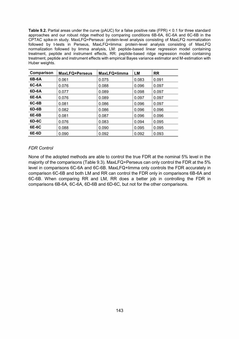
143

Table 9.2. Partial areas under the curve (pAUC) for a false positive rate (FPR) < 0.1 for three standard approaches and our robust ridge method by comparing conditions 6B-6A, 6C-6A and 6C-6B in the CPTAC spike-in study. MaxLFQ+Perseus: protein-level analysis consisting of MaxLFQ normalization followed by t-tests in Perseus, MaxLFQ+limma: protein-level analysis consisting of MaxLFQ normalization followed by limma analysis, LM: peptide-based linear regression model containing treatment, peptide and instrument effects, RR: peptide-based ridge regression model containing treatment, peptide and instrument effects with empirical Bayes variance estimator and M-estimation with Huber weights.

Comparison MaxLFQ+Perseus MaxLFQ+limma LM RR 6B-6A 0.061 0.075 0.083 0.091 6C-6A 0.076 0.088 0.096 0.097 6D-6A 0.077 0.089 0.098 0.097 6E-6A 0.076 0.089 0.097 0.097 6C-6B 0.081 0.086 0.096 0.097 6D-6B 0.082 0.086 0.096 0.096 6E-6B 0.081 0.087 0.096 0.096 6D-6C 0.076 0.083 0.094 0.095 6E-6C 0.088 0.090 0.095 0.095 6E-6D 0.090 0.092 0.092 0.093

FDR Control

None of the adopted methods are able to control the true FDR at the nominal 5% level in the majority of the comparisons (Table 9.3). MaxLFQ+Perseus can only control the FDR at the 5% level in comparisons 6C-6A and 6C-6B. MaxLFQ+limma only controls the FDR accurately in comparison 6C-6B and both LM and RR can control the FDR only in comparisons 6B-6A and 6C-6B. When comparing RR and LM, RR does a better job in controlling the FDR in comparisons 6B-6A, 6C-6A, 6D-6B and 6D-6C, but not for the other comparisons.

144

Table 9.3. Observed FDR when using a 5% FDR cut-off level for each of the three standard approaches and our robust ridge method for all pairwise comparisons between conditions 6A, 6B, 6C, 6D and 6E. MaxLFQ+Perseus: protein-level analysis consisting of MaxLFQ normalization followed by t-tests in Perseus, MaxLFQ+limma: protein-level analysis consisting of MaxLFQ normalization followed by limma analysis, LM: peptide-based linear regression model containing treatment, peptide and instrument effects, RR: peptide-based ridge regression model containing treatment, peptide and instrument effects with empirical Bayes variance estimator and M-estimation with Huber weights. This table shows that most methods are unable to control the FDR at 5%, especially for comparisons involving higher spike-in concentrations (e.g. 6D and 6E).

Comparison MaxLFQ+Perseus MaxLFQ+limma LM RR 6B-6A 0.071 0.048 0.034 0.030 6C-6A 0.040 0.083 0.095 0.050 6D-6A 0.456 0.794 0.466 0.050 6E-6A 0.917 0.922 0.870 0.883 6C-6B 0.037 0 0 0.024 6D-6B 0.640 0.879 0.528 0.494 6E-6B 0.918 0.924 0.863 0.870 6D-6C 0.429 0.799 0.481 0.434 6E-6C 0.886 0.906 0.842 0.848 6E-6D 0.321 0.584 0.386 0.561

2. Case Study

We further illustrate the performance of our novel method on true biological data in which a single trigger was expected to have an impact on several tightly regulated, but highly interconnected pathways. Thus, contrary to a spike-in data set where differential abundance typically heads in one direction (either up or down-regulated) and stays limited to the spiked-in proteins, a biological dataset consists of a plethora of both strongly as well as weakly differentially regulated proteins. Moreover, in the CPTAC data set, the same sample was always used to spike in different amounts of UPS1 proteins in the same yeast background instead of isolating a new yeast proteome each time. Hence, variability in biological repeats will be much larger compared to the spike-in data set. Although detection of differential abundance in real biological data is the ultimate goal, there is no known ground truth available for these data sets and our evaluation is based on visual inspection of selected findings.

We made use of the publicly available data published by Ramond et al. (31) in which the authors compared the proteome of Francisella tularensis mutant for the arginine transporter ArgP to wild-type (WT) bacteria in biological triplicate. For each biological repeat, three technical replicates were also available. We compared the authors' results with the results of our RR method based on the authors-supplied peptides.txt instead of re-searching the raw spectra. In their study, Ramond et al. (31) performed the analysis at the protein level using intensities of at least two different peptides and keeping those proteins with at least 9 out of 18 valid values, and as such analyzed 842 proteins in total. With our approach—analysis at the peptide level and filtering out peptides that appeared only once in the data set—we were able to analyze a total of 989 proteins. Both the results of our ranking as well as the ranking from the original Francisella article can be found in supplemental File S2. When we compared the top 100 proteins with the lowest p values in both methods, only 52 proteins overlapped. Ramond et al. (31) found 309 DA proteins at the 5% FDR level, whereas we only found 159 proteins significantly DA at the same FDR level. Thus, our method appears to be more conservative.





145

We evaluated the differential abundance of the ten proteins that were present in the RR DA list, but not in the original DA list, as well as the ten highest ranked proteins from the original DA list missing in our list. The ten proteins that were only discovered with our method were all lost during the preprocessing procedure of Ramond et al. (31). Among those proteins, six are more highly abundant in the mutant: exodeoxyribonuclease V subunit gamma and ABC transporter membrane protein, as well as four hypothetical proteins (the membrane protein FTN_0835, an AAA+ superfamily member FTN_0274, an alpha/beta hydrolase FTN_0721 and FTN_1244). Four out of the ten proteins that were only discovered by our method have a lower abundance in the mutant. These proteins are Radical SAM superfamily protein, DNA helicase II, C32 tRNA thiolase and the hypothetical protein FTN_0400. Log2 intensity plots of the individual peptide intensities suggest a differential abundance for most of these proteins (supplemental Figs. S14-S23, File S1).

Eight out of the ten highest-ranked proteins in the original DA list all seem to be highly abundant gauged by the number of peptides identified (supplemental Figs. S24-S33, File S1). Further inspection reveals that most of these proteins do not appear to bear strong evidence for DA between WT and mutant. Except for the hypothetical protein FTN_1397 and the Mur ligase family protein, all variance estimates are smaller than 0.01, which leads to extreme T statistics. Empirical Bayesian variance estimation does increase these small variances, but not enough to make them insignificant at the 5% significance level. There seems to be a relatively clear effect for hypothetical protein FTN_1397 (supplemental Fig. S31, File S1), which in our method just did not pass the 5% FDR level (p value of 9.4*10−3 and FDR adjusted p value 0.057). The Mur ligase family protein shows no strong visual DA (supplemental Fig. S32, File S1), but combines a moderate DA estimate (-0.34) with a small variance (0.01). The two other proteins only present in the list of Ramond et al. (31) are rather low-abundant. DNA-binding protein HU-beta (supplemental Fig. S30, File S1) shows no visual evidence for DA at all, but hypothetical protein FTN_1199 (supplemental Fig. S33, File S1) might possess weak evidence for DA.

Ramond et al. (31) also noted that several protein modules had an increased enrichment in DA proteins. In fact, all ribosomal proteins and all proteins involved in branched-chain amino acid (BCAA) synthesis were either unchanged (as the p value did not reach the 5% FDR cut-off) or present in lower amounts in the mutant. Based on their data, one could also suspect an up-regulation of several tricarboxylic acid (TCA) cycle proteins (nine out of 12) in the mutant.

Ribosomal Proteins

It is known that a global down-regulation of ribosome synthesis is a common response to nutrient starvation in Bacteria and Eukarya (47, 48). One might thus expect a similar drop in abundance in the arginine transporter-mutated F. tularensis as its delay in phagosomal escape can be fully restored by supplementation of the medium with excess arginine (31). When considering all 30S and 50S ribosomal proteins (both significant and insignificant in terms of DA), both our method and the original article report log2 FC estimates for 49 ribosomal proteins. As expected, all log2 FC estimates from our method pointed toward down-regulation in the mutant. Contrary, in the analysis of Ramond et al. (31), two proteins, ribosomal protein L7/L12 and 30S ribosomal protein S18 showed, although deemed insignificant, quite large log2 FCs (0.12 resp. 0.54) in favor of up-regulation in the mutant. This again suggest a more stable log2 FC estimation by our method (supplemental Fig. S34, File S1).

BCAA Synthesis Proteins

Based on KEGG, we could only identify nine proteins as BCAA synthesis proteins although the authors report on 12 BCAA synthesis proteins. As we were unable to find the remaining 3 proteins in this pathway, we further focus on nine proteins only. Supplemental Fig. S35, File
















146

S1 shows the distribution of the log2 FC estimates for both the methodology of Ramond et al. (31) and our method. Here, one insignificant protein, dihydroxy-acid dehydratase shows a log2 FC of 0.22. Using our method, all log2 FCs indicate either down-regulation in the mutant (i.e. log2 FCs smaller than 0) or no change at all (log2 FCs smaller than 1*10−17). On average, log2 FC estimates for BCAA synthesis proteins are more negative in our method. Thus, our method provides stronger evidence for down-regulation of some BCAA synthesis proteins in the mutant compared to the method of the original article.

TCA Cycle Proteins

Based on KEGG, we identified 13 TCA cycle proteins, while Ramond et al. (31) reported 12 proteins. When assessing the log2 FC estimates of these authors for the 13 proteins, 10 TCA cycle proteins appear to be up-regulated in the mutant (supplemental Fig. S36, File S1), 8 of which are declared significant. Contrary, in our method, only 1 protein of the TCA cycle (2-oxoglutarate dehydrogenase complex, E2 component, dihydrolipoyltranssuccinase) is found significant. Strikingly, 8 out of 13 TCA cycle proteins even show log2 FC estimates that are in absolute value smaller than 1× 10−9. We therefore zoomed in onthe individual log2 FC estimates of the peptides mapping to these proteins (supplemental Figs. S37-S50, File S1).

2-oxoglutarate dehydrogenase complex, E2 component, dihydrolipoyltranssuccinase (supplemental Fig. S37, File S1) is the only TCA cycle protein that is found at significantly different levels by our analysis. It is also denoted as significant in the original paper's methodology. Nonetheless, the evidence does not seem to be very strong. 2-oxoglutarate dehydrogenase E1 component, dihydrolipoamide acetyltransferase and succinate dehydrogenase iron-sulfur subunit are also denoted as significant in the original analysis with p values of 5.3 × 10−10, 8.1 × 10−4 and 1.1 × 10−3 respectively, although the spectral evidence also appears quite weak (supplemental Figs. S38, S40, and S41, File S1). In our opinion, any visual evidence for differential abundance for malate dehydrogenase, aconitate hydratase, succinyl-CoA synthetase, alpha subunit and isocitrate dehydrogenase is negligible. Nonetheless, p values corresponding to DA for these proteins are estimated at 7.4 × 10−4, 3.6 × 10−3, 0.02 and 0.02 respectively in the paper of Ramond et al. (31) (supplemental Figs. S42, S43, and S47, File S1).

9.1.6. Discussion

In this work, we introduced three extensions to existing peptide-based linear models that significantly improve stability and precision of fold change estimates. These extensions include minimizing a penalized least squares loss function (ridge regression), weighing down outliers via M-estimation with Huber weights and variance stabilization via empirical Bayes. Our estimation approach is inevitably computationally more complex than the linear regression model, albeit much faster than fully Bayesian approaches that have to be fitted by computationally intensive Markov chain Monte Carlo algorithms (49). In this contribution, we normalized log2 transformed peptide intensities using quantile normalization. Many other types of transformation and normalization exist and can be adopted prior to applying our method. Our focus however, is on robust estimation procedures for peptide-based linear models. Therefore, a thorough comparison of preprocessing methods is beyond the scope of this paper.

We compared our novel estimation method to three other methods: a standard protein-level summarization followed by t-tests (MaxLFQ+Perseus), a standard protein-level summarization followed by limma (MaxLFQ+limma) and a peptide-based linear regression model. Evaluation was done based on the CPTAC Study 6 data set, where the ground truth is known as well as on a biological data set, where ArgP mutated versus wild-type Francisella tularensis proteomes












147

are compared. For the CPTAC dataset, we found our method to give more precise and more stable log2 FC estimates for both the yeast null proteins and the spiked-in UPS1 proteins. Thus, our method sufficiently shrinks abundance estimates that are driven by data sparsity in the null proteins, while retaining good DA estimates when sufficient evidence is present (such as for most UPS1 proteins in the CPTAC spike-in study). These findings are supported by theory as ridge regression shrinkage indeed reduces the variability of the estimator and generates overall more precise FC estimates (lower overall RMSE compared to ordinary least squares estimators) (25–27). Furthermore, empirical Bayes variance estimation squeezes the individual residual variances of all models toward a pooled variance which stabilizes the variance estimation. Finally, M-estimation with Huber weights weakens the impact of individual outliers.

The systematic underestimation of the log2 FC estimates provided by our method, even in comparison 6B-6A (Fig. 3), suggests that ionization competition effects can already come into play at spike-in concentration levels of 0.74 fmol/μl (condition 6B). These effects might partly explain why none of the considered methods performs well in controlling the FDR at the nominal 5% level. When analyzing the Francisella dataset, RR is more conservative than the method used by Ramond et al. (31), which might suggest a better protection against false positives. Indeed, ionization competition effects are also relevant for true biological data sets as an increase in a number of highly abundant proteins in a certain condition might generate a downwards bias in peptide intensities corresponding to non-DA proteins in this condition. Researchers should thus carefully reflect whether a low log2 fold change is truly biologically relevant, as ionization suppression effects already seem to appear at low differences in concentration. Indeed, even when disregarding these effects, the abundance of a protein typically has to differ by a reasonable amount to be of interest to a researcher. Therefore, we suggest testing against a minimal log2 FC value that is biologically interesting in a particular experiment; e.g. 0.5 or 1 (50). A similar approach can be easily adopted within our framework, but we have chosen to test against an FC of 0 to make our results comparable with the analysis of Ramond et al. (31).

In practice, only a handful of true positives will typically be selected for further experimental validation. Therefore, the ranking that is produced by a method is more important than its capability to accurately control the FDR at the 5% level. Here, RR produces superior ranking lists compared to all other methods except in comparisons 6D-6A, 6E-6A and 6E-6B, where large ionization suppression effects are expected due to huge spike-in concentration differences. Hence, it will be very difficult to discern the ionization bias from real DA for these comparisons. Each component of our model contributes to an improvement in performance. ROC curves in supplemental Fig. S4, File S1 show that empirical Bayesian variance estimation slightly but consistently improves the performance of the LM model, while M-estimation seems to cause the largest gain (supplemental Fig. S5, File S1). Ridge regression clearly improves the LM model, EB variance estimation slightly improves the ridge regression model while M-estimation again seems to deliver the largest gain in performance. Corresponding AUC and pAUC values can be found in (supplemental Tables S7-S10, File S1).

In the CPTAC case study, we also confirmed that a peptide-based model starting from summed up intensities over different charge states and modifications but corresponding to identical peptide sequences in the same sample (peptides.txt file) tends to have a higher discriminative ability than a model starting from the individual feature intensities (evidence.txt file, see supplemental Fig. S7, File S1). Others have also shown that analysis on the lowest level of summarization does not automatically lead to the best performance (18).



https://www.ncbi.nlm.nih.gov/pmc/articles/PMC4739679/figure/F3/









148

We also applied our method on a biological dataset and compared our results to the performance of the MaxLFQ summarization-based method used in the original publication (31). Proteins identified as DA by our method that were missed in the original publication were all filtered out because too few peptides were identified. Most of these proteins contain relatively strong evidence for DA based on visual inspection of the individual quantile normalized peptide intensities, illustrating that our method can reliably discover DA in proteins that suffer considerably from missing peptides across samples. Proteins which were denoted as DA in the original article but not by our method were typically identified by a lot of peptides but with a weak visual evidence for DA. Indeed, when a lot of peptide intensities are present, modeling at the peptide level does not contribute much to stabilize the overall log2 FC estimate. Mostly though, these small fold changes are not biologically relevant. However, when one seeks DA in sparse data, as is the case in most experiments, our method clearly outperforms classical approaches. We indeed identify possibly interesting effects in low abundant proteins without overfitting, omitting the need for extensive a priori data filtering (e.g. dropping proteins with less than two peptides present in at least nine out of 18 samples as done by Ramond et al. (31)). Consequently, our ability to detect DA in low abundant proteins combined with robustness against irrelevant changes in high abundant proteins is a favorable property.

We also showed that our fold change estimates are more stable for both the ribosomal and the BCAA synthesis modules, which are denoted as DA by Ramond et al. (31). For TCA cycle proteins, nine out of 12 were described as significantly more abundant in the mutant by these authors, while in our method, eight out of 13 TCA cycle proteins have log2 FC estimates that are in absolute value smaller than 1 × 10−9. Upon visual inspection, most of these proteins indeed contain very limited evidence for DA. Our method thus appears to provide more reliable data for follow-up analysis, thereby aiding researchers in drawing more correct conclusions. The fact that almost 82% of the proteins in our DA list of Francisella proteins indeed contain less peptides in the condition with the lowest abundance of this protein, advocates the inclusion of imputation or censoring approaches, or even the combination of our method with estimates derived from spectral counting, which could be used as a rough but very simple validation technique. For example, hypothetical protein FTN_0400 could be a false positive because more peptides are identified in the mutant, although it appears to be less abundant (supplemental Fig. S18, File S1). This could be an indication of intensity-dependent censoring in the WT. Just like the peptide-based linear regression model, our RR model can handle missing values. The models we presented here assume missingness completely at random, an assumption that is flawed when analyzing shotgun proteomics data. Note, however, that peptide-based models partially correct for this by incorporating peptide-specific effects. Moreover, our strategies to improve robustness of the estimators can be easily plugged into censored regression methods or estimation approaches that adopt advanced imputation techniques for handling missing data (40).

Another interesting outlook is to model all proteins together by incorporating pathway or module level effects in the model in order to make stronger inferences on individual proteins belonging to a certain pathway. Finally, we want to stress the importance of data exploration. Plots of log2 peptide intensities for proteins that are flagged as differential abundant are very useful for assessing the biological relevance and the degree of belief one can have in the DA proteins that are returned by a method.

We are currently preparing an R/Bioconductor package for our method. Meanwhile, all code and data needed to repeat the data analysis in this manuscript is available in Supplemental File 3.








149

9.1.7. Footnotes

Author contributions: L.J.G. and L.C. designed research; L.J.G. and L.C. performed research; L.J.G. analyzed data; L.J.G., K.G., and L.C. wrote the paper.

* This research was supported in part by IAP research network “StUDyS” grant no. P7/06 of the Belgian government (Belgian Science Policy) and the Multidisciplinary Research Partnership “Bioinformatics: from nucleotides to networks” of Ghent University. L.G. is supported by a Ph.D. grant from the Institute for the Promotion of Innovation through Science and Technology in Flanders (IWT-Vlaanderen) entitled “Differential proteomics at peptide, protein and module level” (141573).

This article contains supplemental Files S1 to S3.

9.1.8. References

1. Oda Y., Huang K., Cross F. R., Cowburn D., and Chait B. T. (1999) Accurate quantitation of protein expression and site-specific phosphorylation. Proc. Natl. Acad. Sci. U.S.A. 96, 6591–6596

2. Ong S.-E., Blagoev B., Kratchmarova I., Kristensen D. B., Steen H., Pandey A., and Mann M. (2002) Stable isotope labeling by amino acids in cell culture, SILAC, as a simple and accurate approach to expression proteomics. Mol. Cell. Proteomics 1, 376–386

3. Gygi S. P., Rist B., Gerber S. A., Turecek F., Gelb M. H., and Aebersold R. (1999) Quantitative analysis of complex protein mixtures using isotope-coded affinity tags. Nat. Biotech. 17, 994–999

4. Hsu J.-L., Huang S.-Y., Chow N.-H., and Chen S.-H. (2003) Stable-isotope dimethyl labeling for quantitative proteomics. Anal. Chem. 75, 6843–6852

5. Ross P. L., Huang Y. N., Marchese J. N., Williamson B., Parker K., Hattan S., Khainovski N., Pillai S., Dey S., Daniels S., Purkayastha S., Juhasz P., Martin S., Bartlet-Jones M., He F., Jacobson A., and Pappin D. J. (2004) Multiplexed protein quantitation in Saccharomyces cerevisiae using amine-reactive isobaric tagging reagents. Mol. Cell. Proteomics 3, 1154–1169

6. Thompson A., Schäfer J., Kuhn K., Kienle S., Schwarz J., Schmidt G., Neumann T., and Hamon C. (2003) Tandem mass tags: A novel quantification strategy for comparative analysis of complex protein mixtures by MS/MS. Anal. Chem. 75, 1895–1904

7. Bantscheff M., Schirle M., Sweetman G., Rick J., and Kuster B. (2007) Quantitative mass spectrometry in proteomics: a critical review. Anal. Bioanal. Chem. 389, 1017–1031

8. Patel V. J., Thalassinos K., Slade S. E., Connolly J. B., Crombie A., Murrell J. C., and Scrivens J. H. (2009) A comparison of labeling and label-free mass spectrometry-based proteomics approaches. J. Proteome Res. 8, 3752–3759

9. Rodriguez J., Gupta N., Smith R. D., and Pevzner P. A. (2008) Does trypsin cut before proline? J. Proteome Res. 7, 300–305

10. Abaye D. A., Pullen F. S., and Nielsen B. V. (2011) Peptide polarity and the position of arginine as sources of selectivity during positive electrospray ionisation mass spectrometry. Rapid Commun. Mass Spectrom. 25, 3597–3608


150

11. Schliekelman P., and Liu S. (2013) Quantifying the effect of competition for detection between coeluting peptides on detection probabilities in mass-spectrometry-based proteomics. J. Proteome Res. 13, 348–361

12. Venable J. D., Dong M.-Q., Wohlschlegel J., Dillin A., and Yates J. R. (2004) Automated approach for quantitative analysis of complex peptide mixtures from tandem mass spectra. Nat. Meth. 1, 39–45

13. Gillet L. C., Navarro P., Tate S., Röst H., Selevsek N., Reiter L., Bonner R., and Aebersold R. (2012) Targeted data extraction of the MS/MS spectra generated by data-independent acquisition: A new concept for consistent and accurate proteome analysis. Mol. Cell. Proteomics 11, 1–17

14. Bilbao A., Varesio E., Luban J., Strambio-De-Castillia C., Hopfgartner G., Müller M., and Lisacek F. (2015) Processing strategies and software solutions for data-independent acquisition in mass spectrometry. Proteomics 15, 964–980

15. Liu H., Sadygov R. G., and Yates J. R. (2004) A Model for Random Sampling and Estimation of Relative Protein Abundance in Shotgun Proteomics. Anal. Chem. 76, 4193–4201

16. Old W. M., Meyer-Arendt K., Aveline-Wolf L., Pierce K. G., Mendoza A., Sevinsky J. R., Resing K. A., and Ahn N. G. (2005) Comparison of label-free methods for quantifying human proteins by shotgun proteomics. Mol. Cell. Proteomics 4, 1487–1502

17. Bantscheff M., Lemeer S., Savitski M., and Kuster B. (2012) Quantitative mass spectrometry in proteomics: critical review update from 2007 to the present. Anal. Bioanal. Chem. 404, 939–965

18. Milac T. I., Randolph T. W., and Wang P. (2012) Analyzing LC-MS/MS data by spectral count and ion abundance: two case studies. Statistics Interface 5, 75–87

19. Krey J. F., Wilmarth P. A., Shin J.-B., Klimek J., Sherman N. E., Jeffery E. D., Choi D., David L. L., and Barr-Gillespie P. G. (2014) Accurate label-free protein quantitation with high- and low-resolution mass spectrometers. J. Proteome Res. 13, 1034–1044

20. Zhang Y., Fonslow B. R., Shan B., Baek M.-C., and Yates J. R. (2013) Protein analysis by shotgun/bottom-up proteomics. Chem. Rev. 113, 2343–2394

21. Goeminne L. J. E., Argentini A., Martens L., and Clement L. (2015) Summarization vs peptide-based models in label-free quantitative proteomics: Performance, pitfalls, and data analysis guidelines. J. Proteome Res. 14, 2457–2465

22. Clough T., Key M., Ott I., Ragg S., Schadow G., and Vitek O. (2009) Protein quantification in label-free LC-MS experiments. J. Proteome Res. 8, 5275–5284

23. Karpievitch Y. V., Dabney A. R., and Smith R. D. (2012) Normalization and missing value imputation for label-free LC-MS analysis. BMC Bioinformatics 13, S5.

24. Ting L., Cowley M. J., Hoon S. L., Guilhaus M., Raftery M. J., and Cavicchioli R. (2009) Normalization and statistical analysis of quantitative proteomics data generated by metabolic labeling. Mol. Cell. Proteomics 8, 2227–2242

25. Ahmed S. E., and Raheem S. M. E. (2012) Shrinkage and absolute penalty estimation in linear regression models. Computational Stat. 4, 541–553

26. Stein C. (1956) Inadmissibility of the usual estimator for the mean of a multivariate normal distribution. Proceedings of the Third Berkeley Symposium on Mathematical Statistics and

151

Probability, Volume 1: Contributions to the Theory of Statistics, pp. 197–206, University of California Press, Berkeley, Calif.

27. Copas J. B. (1983) Regression, prediction and shrinkage. J. Roy. Statist. Soc.. 45, 311–354

28. Huber P. J. (1964) Robust estimation of a location parameter. The Annals of Mathematical Statistics. 35, 73–101

29. Paulovich A. G., Billheimer D., Ham A.-J. L., Vega-Montoto L., Rudnick P. A., Tabb D. L., Wang P., Blackman R. K., Bunk D. M., Cardasis H. L., Clauser K. R., Kinsinger C. R., Schilling B., Tegeler T. J., Variyath A. M., Wang M., Whiteaker J. R., Zimmerman L. J., Fenyo D., Carr S. A., Fisher S. J., Gibson B. W., Mesri M., Neubert T. A., Regnier F. E., Rodriguez H., Spiegelman C., Stein S. E., Tempst P., and Liebler D. C. (2010) Interlaboratory study characterizing a yeast performance standard for benchmarking LC-MS platform performance. Mol. Cell. Proteomics 9, 242–254

30. Cox J., and Mann M. (2008) MaxQuant enables high peptide identification rates, individualized p.p.b.-range mass accuracies and proteome-wide protein quantification. Nat. Biotechnol. 26, 1367–1372

31. Ramond E., Gesbert G., Guerrera I. C., Chhuon C., Dupuis M., Rigard M., Henry T., Barel M., and Charbit A. (2015) Importance of host cell arginine uptake in Francisella phagosomal escape and ribosomal protein amounts. Mol. Cell. Proteomics 14, 870–881

32. Cox J., Hein M. Y., Luber C. A., Paron I., Nagaraj N., and Mann M. (2014) Accurate proteome-wide label-free quantification by delayed normalization and maximal peptide ratio extraction, termed MaxLFQ. Mol. Cell. Proteomics 13, 2513–2526

33. R Core Team (2014) R: A language and environment for statistical computing. R Foundation for Statistical Computing, Vienna, Austria

34. Ritchie M. E., Phipson B., Wu D., Hu Y., Law C. W., Shi W., and Smyth G. K. (2015) limma powers differential expression analyses for RNA-sequencing and microarray studies. Nucleic Acids Res. 43, e47.

35. Amaratunga D., and Cabrera J. (2001) Analysis of data from viral DNA microchips. J. Am. Statist. Assoc. 96, 1161–1170

36. Bolstad B. M., Irizarry R. A., Åstrand M., and Speed T. P. (2003) A comparison of normalization methods for high density oligonucleotide array data based on variance and bias. Bioinformatics 19, 185–193

37. Callister S. J., Barry R. C., Adkins J. N., Johnson E. T., Qian W.-j., Webb-Robertson B.-J. M., Smith R. D., and Lipton M. S. (2006) Normalization approaches for removing systematic biases associated with mass spectrometry and label-free proteomics. J. Proteome Res. 5, 277–286

38. Rudnick P. A., Wang X., Yan X., Sedransk N., and Stein S. E. (2014) Improved normalization of systematic biases affecting ion current measurements in label-free proteomics data. Mol. Cell. Proteomics 13, 1341–1351

39. Daly D. S., Anderson K. K., Panisko E. A., Purvine S. O., Fang R., Monroe M. E., and Baker S. E. (2008) Mixed-effects statistical model for comparative LC-MS proteomics studies. J. Proteome Res. 7, 1209–1217

152

40. Karpievitch Y., Stanley J., Taverner T., Huang J., Adkins J. N., Ansong C., Heffron F., Metz T. O., Qian W.-J., Yoon H., Smith R. D., and Dabney A. R. (2009) A statistical framework for protein quantitation in bottom-up MS-based proteomics. Bioinformatics 25, 2028–2034

41. Ruppert D., Wand M. P., and Carroll R. J. (2003) Semiparametric Regression, Cambridge University Press, New York

42. Bates D M. M., Bolker BM, Walker S. (2014) lme4: Linear mixed-effects models using Eigen and S4. J. Statistical Software 67, 1–48

43. Lönnstedt I., and Speed T. (2002) Replicated microarray data. Statistica Sinica 12, 31–46

44. Smyth G. K. (2004) Linear models and empirical bayes methods for assessing differential expression in microarray experiments. Stat. Appl. Genet. Mol. Biol. 3, Article3

45. Benjamini Y., and Hochberg Y. (1995) Controlling the false discovery rate: A practical and powerful approach to multiple testing. J. Royal Statist. Soc. 57, 289–300

46. Schwämmle V., León I. R., and Jensen O. N. (2013) Assessment and improvement of statistical tools for comparative proteomics analysis of sparse data sets with few experimental replicates. J. Proteome Res. 12, 3874–3883

47. Rudra D., and Warner J. R. (2004) What better measure than ribosome synthesis? Genes Dev. 18, 2431–2436

48. Dressaire C., Redon E., Gitton C., Loubiere P., Monnet V., and Cocaign-Bousquet M. (2011) Investigation of the adaptation of Lactococcus lactis to isoleucine starvation integrating dynamic transcriptome and proteome information. Microbial Cell Factories 10, S18.

49. Henao R., Thompson J. W., Moseley M. A., Ginsburg G. S., Carin L., and Lucas J. E. (2012) Hierarchical factor modeling of proteomics data. Computational Advances in Bio and Medical Sciences (ICCABS), 2012 IEEE 2nd International Conference on, pp. 1–6

50. McCarthy D. J., and Smyth G. K. (2009) Testing significance relative to a fold-change threshold is a TREAT. Bioinformatics 25, 765–771

9.1.9. Appendix

Ridge regression

The untransformed, preprocessed intensities for each peptide 𝑝 in each run 𝑟 are assumed to follow a log-normal distribution. After log-transformation, these intensities become normally distributed. In all generality, for each protein, we propose the following peptide-based regression model that has also been proposed by Daly et al. (2008) [1]:

𝑦𝑝𝑟 = 𝒙𝑝𝑟𝜷 + 𝛽𝑝peptide + 𝑢𝑟

run + 𝜀𝑝𝑟

Herein, 𝒙𝑝𝑟 is a row matrix with the covariate pattern related to peptide 𝑝 in run 𝑟, 𝜷 =

[𝛽0, 𝛽11 … , 𝛽𝑚1

1 … , 𝛽𝑀11 , … , 𝛽𝑚𝑔

𝑔 ,… , 𝛽𝑀𝑔𝑔 , … , 𝛽𝑀𝐺

𝐺 ]T is a vector with 1 + 𝑀 = 1 + ∑ 𝑀𝑔

𝐺𝑔=1

parameters denoting the effects of 𝑀 predictors corresponding to 𝐺 covariates. 𝛽𝑝peptide is a

peptide-specific effect for peptide 𝑝, 𝑢𝑟run a random run effect to account for within-run

correlation, with 𝑢𝑟run~N(0, 𝜎𝑢

2). 𝜀𝑝𝑟~N(0, 𝜎2) is a random error term.

We now want to introduce an extra penalization on the fixed effects beta by exploiting the link between ridge regression and mixed models (see section 4.2.4). Except for a fixed intercept

153

𝛽0, we penalize the parameters corresponding to each covariate group 𝑔 by assuming: 𝛽𝑚𝑔

𝑔 ~N(0, 𝜎2 𝜆𝑔⁄ ) for 𝑚𝑔 = 1,… ,𝑀𝑔. Herein, 𝑔 refers to the 𝑔th covariate and accounts for the fact that certain covariates are modeled with more than one parameter. For example, a treatment effect with three levels will be modeled with three dummy parameters 𝛽1

treatment, 𝛽2

treatment, and 𝛽3treatment whereby 𝛽1

treatment + 𝛽2treatment + 𝛽3

treatment = 0. We also assume

𝛽𝑝peptide~N(0, 𝜎2 𝜆peptide⁄ ). Therefore, the BLUP estimator for [

𝜷𝜷peptide

𝒖run] can be written as

follows:

[�̂�

�̂�peptide

�̂�run] = (𝑪T𝑪 + 𝑩)−1𝑪T𝒚

With 𝒚 =

[ 𝑦11…𝑦1𝑅…𝑦𝑝𝑟…𝑦𝑃1…𝑦𝑃𝑅]

and 𝑪 =

[ 𝒙11…𝒙1𝑅…𝒙𝑝𝑟…

𝒙𝑃1…𝒙𝑃𝑅

𝒙1peptide…

𝒙1peptide…

𝒙𝑝peptide

…𝒙𝑃

peptide…

𝒙𝑃peptide

𝒙1run…

𝒙𝑅run…

𝒙𝑟run

…𝒙1

run…

𝒙𝑅run

]

. Herein 𝒙𝑝peptide is a row vector of dummies, for

which the 𝑝th element is equal to 1 and all other elements equal to 0. 𝒙𝑟run is a row vector of

dummies with the 𝑟th element equal to 1 and all other elements equal to 0. 𝑩 is an (1 + 𝑀 +𝑃 + 𝑅) × (1 + 𝑀 + 𝑃 + 𝑅) diagonal matrix with diagonal elements [0 𝒈 𝒑 𝒓], with 𝒈 a vector of length 𝑀 containing the 𝜆𝑔 that corresponds to each parameter estimate �̂�𝑚𝑔

𝑔 for 𝑚𝑔 = 1,… ,𝑀𝑔 and 𝑔 = 1,… , 𝐺, 𝒑 a vector of length 𝑃 containing the 𝜆peptide that corresponds to each

parameter estimate �̂�𝑝peptide for 𝑝 = 1,… , 𝑃 and 𝒓 a vector of length 𝑅 containing the �̂�𝑢

2

�̂�2 that corresponds to each parameter estimate �̂�𝑟

run for 𝑟 = 1,… , 𝑅.

Robust regression with M estimation

To robustify our procedure against outliers, we use a weighted maximum likelihood method with Huber weights, as proposed by Zhou (2009) [2].

∑𝑤𝑗

𝐽

𝑗=1

l(𝑦𝑗, 𝜷, 𝒖),

with 𝑗 = 1,… , 𝐽 an indicator for observation. This weighted log-likelihood is solved iteratively. The mixed model is fitted while the weights are kept constant. Then, the weights are recomputed using Huber’s weight function on the residuals scaled with the residual standard deviation. This procedure is repeated until convergence. After convergence, the weighted BLUP estimator is given by:

[�̂�

�̂�peptide

�̂�run] = (𝑪T𝑾𝑪 + 𝑩)−1𝑪T𝑾𝒚,

with 𝑾 = [𝑤1 …𝑤𝑗 …𝑤𝐽]𝑰𝐽×𝐽 and 𝑤1 to 𝑤𝐽 the weights corresponding to these observations and 𝑰𝐽×𝐽 a 𝐽 × 𝐽 unity matrix. Zhou (2009) [2] showed that the weighted BLUP estimator is better

154

than the unweighted one in terms of bias and efficiency when the data contains some outliers but provides the same asymptotic efficiency when the model is correctly specified. Robust M estimation with Huber weights has also been used to robustify the negative binomial model in the popular RNA sequencing R package EdgeR [3].

Empirical Bayes variance estimation

Finally, we robustify our inference with limma’s empirical Bayes variance estimation (see section 4.2.2). In brief, limma assumes the following prior distribution on the error variance 𝜎𝑖

2 for each protein 𝑖 (𝑖 = 1,… , 𝐼):

1𝜎𝑖

2 ~1

𝑑0𝜎02 𝜒𝑑0

2 ,

with 𝜎02 a prior variance and 𝜒𝑑0

2 a 𝜒2 distribution with 𝑑0 degrees of freedom. A maximum a posteriori residual standard deviation �̃�𝑖 for each protein is given by:

�̃�𝑖 = √𝑑𝑖�̂�𝑖2 + 𝑑0�̂�0

2

𝑑𝑖 + 𝑑0

We then plug in this posterior residual standard deviation in the estimator for the standard deviation of the model parameter of interest, �̂�𝑚𝑔

𝑔 (suppressing the indicator 𝑖 for notational convenience):

�̃��̂�𝑚𝑔𝑔 = �̃�√(𝑪T𝑾𝑪 + 𝑩)𝑚𝑔,𝑚𝑔

−1

Herein, 𝑚𝑔,𝑚𝑔 denotes the 𝑚𝑔th diagonal element of the matrix. This enables statistical inference with a moderated t-test with 𝑑𝑖 + 𝑑0 degrees of freedom:

�̃�𝑖𝑚𝑔 =�̂�𝑖𝑚𝑔

𝑔

�̃��̂�𝑖𝑚𝑔𝑔

Herein, 𝑑𝑖 is calculated as 𝐽 − 𝑡𝑟(𝑯), with 𝐽 the total number of observations and 𝑯 the hat matrix, which is calculated as follows:

𝑯 = 𝑪(𝑪T𝑾𝑪 + 𝑩)−1𝑪T𝑾

Implementation

MSqRob builds on the lme4 R package for parameter estimation and statistical inference [4]. Shrinkage on fixed effect parameters is obtained by encoding them as random effects. To allow for robust M-estimation, a loop is placed around the model fitting procedure: after model fitting, Huber weights are calculated on the residuals scaled with the residual standard deviation. These weights are provided as arguments to the lmer function of the lme4 package, which allows to estimate the parameters via weighted log-likelihood. This procedure is repeated until convergence.

References for the Appendix

1. Daly, D.S. et al., Mixed-Effects Statistical Model for Comparative LC−MS Proteomics Studies. Journal of Proteome Research, 2008. 7(3): p. 1209-1217.

2. Zhou, T., Weighting Method for a Linear Mixed Model. Communications in Statistics - Theory and Methods, 2009. 39(2): p. 214-227.

155

3. Zhou, X., H. Lindsay, and M.D. Robinson, Robustly detecting differential expression in RNA sequencing data using observation weights. Nucleic Acids Research, 2014. 42(11): p. e91-e91.

4. Bates, D. et al., Fitting Linear Mixed-Effects Models Using lme4. Journal of Statistical Software; Vol 1, Issue 1 (2015), 2015.

statistical methods for differential proteomics at …

Documents