statistical modeling of simulation errors and their reduction via response surface techniques
TRANSCRIPT

STATISTICAL MODELING OF SIMULATION ERRORS AND THEIR REDUCTION VIA RESPONSE
SURFACE TECHNIQUES
By
Hongman Kim
A DISSERTATION SUBMITTED TO THE FACULTY OF THE
VIRGINIA POLYTECHNIC INSTITUTE AND STATE UNIVERSITY
IN PARTIAL FULFILLMENT OF THE REQUIREMENTS FOR THE DEGREE OF
DOCTOR OF PHILOSOPHY
IN
AEROSPACE ENGINEERING
William H. Mason, Chairman
Raphael T. Haftka Layne T. Watson
Bernard Grossman Eugene M. Cliff
June 18, 2001
Blacksburg, Virginia
Keywords: discretization error, convergence error, response surface technique, Weibull distribution, M-estimation
STATISTICAL MODELING OF SIMULATION ERRORS AND THEIR
REDUCTION VIA RESPONSE SURFACE TECHNIQUES
By
Hongman Kim
Committee Chairman: William H. Mason
Aerospace Engineering
(ABSTRACT)
Errors of computational simulations in design of a high-speed civil transport (HSCT) are
investigated. First, discretization error from a supersonic panel code, WINGDES, is considered.
Second, convergence error from a structural optimization procedure using GENESIS is
considered along with the Rosenbrock test problem.
A grid converge study is performed to estimate the order of the discretization error in the
lift coefficient (CL) of the HSCT calculated from WINGDES. A response surface (RS) model
using several mesh sizes is applied to reduce the noise magnification problem associated with the
Richardson extrapolation. The RS model is shown to be more efficient than Richardson
extrapolation via careful use of design of experiments.
A programming error caused inaccurate optimization results for the Rosenbrock test
function, while inadequate convergence criteria of the structural optimization produced error in
wing structural weight of the HSCT. The Weibull distribution is successfully fit to the
optimization errors of both problems. The probabilistic model enables us to estimate average
errors without performing very accurate optimization runs that can be expensive, by using
differences between two sets of results with different optimization control parameters such as
initial design points or convergence criteria.
Optimization results with large errors, outliers, produced inaccurate RS approximations.
A robust regression technique, M-estimation implemented by iteratively reweighted least squares
(IRLS), is used to identify the outliers, which are then repaired by higher fidelity optimizations.

iii
The IRLS procedure is applied to the results of the Rosenbrock test problem, and wing structural
weight from the structural optimization of the HSCT. A nonsymmetric IRLS (NIRLS), utilizing
one-sidedness of optimization errors, is more effective than IRLS in identifying outliers.
Detection and repair of the outliers improve accuracy of the RS approximations. Finally,
configuration optimizations of the HSCT are performed using the improved wing bending
material weight RS models.

iv
Acknowledgements
During the last four years, the MDO research group at Virginia Tech has provided me
with a unique educational environment. Close cooperation with devoted professors and many
talented students helped me broaden academic and professional perspectives.
I spent a lot of time in the office of Dr. William Mason, my adviser, to discuss many
challenging problems we faced in the research. I remember that his office was a busy place
because there were always many students who wanted to ask him questions. His passion and
expertise in aircraft design have been a real treat to me and I’m deeply grateful for his
continuous support and encouragements.
I would like to express my deepest thanks to Dr. Raphael Haftka at the University of
Florida for his enormous help and encouragements. The geographical distance was not a match
to his passion for research and teaching. The weekly teleconferences, numerous email
correspondences, and chances of face-to-face talk with him always provided me with new
perspectives on the subject. I’m very grateful to Dr. Bernard Grossman for his support and
encouragements. He offered fresh suggestions to my work and it was a pleasure to work with
him. Dr. Layne Watson helped me a lot by sharing his expertise in mathematics and statistics.
Many chances of discussion with him were valuable assets to me. Dr. Eugene Cliff offered very
insightful discussions, and I appreciate his efforts in the committee.
I would like to express special thanks to Dr. Jeffrey Birch in the Department of Statistics
at Virginia Tech, who introduced me to the world of applied statistics. I really enjoyed his
classes, where I learned many ideas used in this work. Dr. Chris Roy at Sandia National
Laboratory offered valuable comments on the issues of discretization error, and his contributions
are appreciated.
It was a great pleasure to work with many gentlemen, my colleague graduate students in
Virginia Tech and the University of Florida. In particular, contributions from Chuck Baker and
Melih Papila are appreciated. Close presence of Sangmook Shin and Yongwook Kim was always
a great help to me. I received a lot from brothers and sisters of the Korean Baptist Church of
Blacksburg, and I would like to give special thanks to the single bible study group for our
fellowship in Jesus Christ.

v
I could not be here without love and support of my family. Very special love goes to my
grandmother. She was my first friend. Thanks from my heart goes to my sister and brother’s
family, who were together in pleasant and difficult times of life. I would like to express my
deepest love to my father, who showed me endless support and love. Finally, I would like to
share the joy of this small achievement with my mother who rests in heaven with the Lord.

vi
Table of Contents
Acknowledgements ...................................................................................................................... iv
Table of Contents ......................................................................................................................... vi
List of Tables ................................................................................................................................ ix
List of Figures............................................................................................................................... xi
Nomenclature ............................................................................................................................. xiii
Chapter 1 Introduction................................................................................................................. 1
1.1 Motivation............................................................................................................................. 1
1.2 Review of the Literature ....................................................................................................... 2
1.3 Objective............................................................................................................................... 6
1.4 Methodology......................................................................................................................... 7
1.5 Outline .................................................................................................................................. 9
Chapter 2 HSCT Configuration Design Optimization Problem ............................................ 12
2.1 Formulation of the Problem................................................................................................ 12
2.2 Analysis Methods and Tools............................................................................................... 13
2.2.1 Aerodynamic Analysis................................................................................................. 13
2.2.2 Weight and Structural Analysis ................................................................................... 14
Chapter 3 Examples of Simulation Errors in HSCT Design .................................................. 20
3.1 Supersonic Aerodynamic Analysis Using WINGDES....................................................... 20
3.2 Structural Optimization....................................................................................................... 22
Chapter 4 Response Surface Methodology............................................................................... 28
4.1 Design of Experiments........................................................................................................ 28
4.2 Least Squares Fit................................................................................................................. 29
4.3 Analysis of Variance........................................................................................................... 31
4.4 Noise of Simulation Data and RS Fit.................................................................................. 32
Chapter 5 Probabilistic Modeling of Simulation Errors......................................................... 33
5.1 Overview of Probabilistic Modeling of Errors ................................................................... 33
vii
5.2 Model Distribution Functions............................................................................................. 35
5.3 Maximum Likelihood Estimate of Model Distribution ...................................................... 35
5.4 χ2 Goodness-of-Fit Test...................................................................................................... 36
5.5 Probability Plot ................................................................................................................... 37
5.6 Indirect Fit of Error Distribution using Differences of Simulation Results........................ 38
Chapter 6 Robust Regression Techniques and Outlier Detection.......................................... 43
6.1 Iteratively Reweighted Least Squares................................................................................. 43
6.2 Nonsymmetric IRLS (NIRLS)............................................................................................ 46
Chapter 7 RS Modeling of Errors from Supersonic Aerodynamic Simulation.................... 52
7.1 Grid Convergence Study of WINGDES............................................................................. 53
7.2 Higher Order Formulas using Richardson Extrapolation ................................................... 54
7.2.1 Extrapolation for h = 0................................................................................................. 54
7.2.2 Extrapolation for Finite Mesh Sizes............................................................................. 55
7.3 RS Modeling of Discretization Error.................................................................................. 56
7.3.1 Incorporating Discretization Error into the RS Model ................................................ 57
7.3.2 Comparison between Richardson Extrapolation and RS Approach ............................ 57
7.3.3 RS Fit to the Data from Richardson Extrapolation...................................................... 59
Chapter 8 Test Problem Study of Errors from Optimization Failures ................................. 67
8.1 Errors of Various Optimization Methods on the Rosenbrock Function ............................. 67
8.2 Parameterized Rosenbrock function ................................................................................... 68
8.3 Estimation of the Optimization Error ................................................................................. 70
8.3.1 Homogeneity of the Error Distribution........................................................................ 70
8.3.2 Results of Direct Fit of PORT Optimization Error ...................................................... 71
8.3.3 Results of Indirect Fit of PORT Optimization Error ................................................... 72
8.4 Detection and Repair of Erroneous Optimization Runs ..................................................... 73
8.5 Effects of Outlier Repair on the Quality of the Optimum of RS Approximation............... 74
Chapter 9 Estimation of Error from Structural Optimization .............................................. 85
9.1 Effects of Convergence Control Parameters on the Optimization Error ............................ 85
9.2 Estimation of Statistical Distribution.................................................................................. 88
9.2.1 Homogeneity of Error .................................................................................................. 88
9.2.2 Direct Fit of Estimated Error ....................................................................................... 89

viii
9.2.3 Results of Indirect Fit of the Optimization Error......................................................... 91
Chapter 10 Detection and Repair of Poorly Converged Structural Optimization Runs ... 110
10.1 IRLS Procedures for the Optimization Error: Symmetric and Non-symmetric Weighting
Functions................................................................................................................................. 110
10.2 Results of Outlier Detection and Repair ......................................................................... 111
10.3 Advantage of Outlier Repair over Exclusion.................................................................. 113
10.4 Improvement of Wing Structural Weight RS Approximations Using Repaired Data.... 113
10.5 HSCT Configuration Optimization Using Improved Wb RS Approximations ............... 114
Chapter 11 Conclusions............................................................................................................ 125
Bibliography .............................................................................................................................. 127
Appendix A Design of Experiments ........................................................................................ 136
A.1 Full Factorial Design........................................................................................................ 136
A.2 Centered Composite Design (CCD)................................................................................. 136
A.3 D-optimal Design............................................................................................................. 137
Appendix B Failure Rate of the Weibull Distribution........................................................... 138
Appendix C Numerical Integration of Joint Probability Distribution of the Weibull Models
..................................................................................................................................................... 140
Appendix D Experimental Design of HSCT and Ws Data..................................................... 142
Appendix E MATLAB Code for Direct Fit of Weibull Model to Optimization Errors..... 144
Appendix F MATLB Code for Indirect Fit of Weibull Model to Optimization Errors..... 148
Appendix G SAS Input File for IRLS Procedure .................................................................. 152
VITA........................................................................................................................................... 156

ix
List of Tables
Table 2.1: Twenty-nine configuration design variables for HSCT............................................... 15
Table 2.2: Constraints for the HSCT design. ................................................................................ 16
Table 2.3: The simplified version of the HSCT design with five configuration variables. .......... 17
Table 3.1: Computational time for supersonic aerodynamic analysis of HSCT using WINGDES
according to panel step sizes....................................................................................... 24
Table 3.2: Load cases for the structural optimization of HSCT. .................................................. 24
Table 5.1: Examples of model functions for continuous distribution........................................... 41
Table 6.1: Weighting functions of M-estimator............................................................................ 48
Table 7.1: Estimates of order of error convergence of CL from WINGDES. ............................... 61
Table 7.2: Error in CL (ny = 320) prediction of the Richardson extrapolation. ............................. 62
Table 7.3: Error in CL (ny = 320) prediction of the RS model....................................................... 62
Table 7.4: Error in CL (ny = 320) prediction of the RS fit to the Richardson extrapolation results.
..................................................................................................................................... 62
Table 8.1: Failure of various optimization programs for the five dimensional Rosenbrock
function. ...................................................................................................................... 75
Table 8.2: Summary of PORT runs for 125 variants of the parameterized Rosenbrock function.75
Table 8.3: Fits of the Weibull model to the error from PORT optimization of the parameterized
Rosenbrock function. .................................................................................................. 76
Table 8.4: Results of the indirect fit for the optimization error of PORT. ................................... 77
Table 8.5: Comparison of the estimates of mean ( fitµ ) and the estimates of standard deviation
( fitσ ) from indirect fit with dataµ and dataσ (see Eq. 8.5)........................................... 78
Table 8.6: Results of outlier repair for the parameterized five dimensional Rosenbrock function.
..................................................................................................................................... 78
Table 8.7: Results of optimization of fo(b1, b2, b3) from the parameterized Rosenbrock function
using RS approximations before and after outlier repair. ........................................... 79
Table 9.1: Sets of optimization control parameters in GENESIS................................................. 94
Table 9.2: Performance of structural optimization for various GENESIS parameter settings. .... 95

x
Table 9.3: Quality of the fit of the Weibull model to the optimization error, et, for various
convergence settings defined in Table 9.1. ................................................................. 96
Table 9.4: Quality of fit of the Weibull model to the relative optimization error scaled with
respect to Ws................................................................................................................ 97
Table 9.5: Correlation coefficients of the estimated errors (et, lb.) between different GENESIS
parameter settings. ...................................................................................................... 98
Table 9.6: Results of the difference fits for the pair of (A2, A3) and the pair of (A2, B2). ......... 98
Table 9.7: Comparison of the estimates of mean (fitµ ) and the estimates of standard deviation
(fitσ ) from indirect fit with the estimates from data (
dataµ and dataσ , see Eq. 9.1). ...... 99
Table 10.1: Performance of structural optimization for various GENESIS parameter settings. 116
Table 10.2: Results of outlier repair for Case A2. ...................................................................... 117
Table 10.3: Results of outlier repair for Case B2. ...................................................................... 118
Table 10.4: Results of five variable configuration optimizations using Wb RS before and after
outlier repair (Based on data of Case B2). ................................................................ 119

xi
List of Figures
Figure 2.1: Design variables of the 29 variable HSCT design. .................................................... 18
Figure 2.2: Design variables of the five variable HSCT design. .................................................. 19
Figure 3.1: Panel system of WINGDES (from Ref. [54]). ........................................................... 25
Figure 3.2: Variation of lift coefficient, CL, with wing tip chord for various panel sizes (M = 2.4,
α = 2.292°)................................................................................................................. 25
Figure 3.3: Typical FE mesh for the structural optimizations. ..................................................... 26
Figure 3.4: Noisy results from HSCT structural optimization and repaired results using tightened
convergence criteria................................................................................................... 27
Figure 5.1: Probability density functions for Gaussian with µ = 0 and various σ........................ 42
Figure 5.2: Probability density functions for Weibull with β = 1 and various α.......................... 42
Figure 6.1: Various weighting functions of the M-estimator........................................................ 49
Figure 6.2: The corresponding ψ functions of the M-estimator. .................................................. 49
Figure 6.3: One-dimensional example of outlier detection by IRLS............................................ 50
Figure 6.4: Flow chart of the IRLS/NIRLS procedure for low fidelity optimization data. .......... 51
Figure 7.1: Grid convergence study of CL from WINGDES (M = 2.4, α = 2.292°). ................... 63
Figure 7.2: Comparison of CL prediction for h = 0 between Richardson extrapolation (RE) and
RS model. .................................................................................................................. 64
Figure 7.3: Comparison of CL prediction for ny = 320 between Richardson extrapolation (RE) and
RS model. .................................................................................................................. 65
Figure 7.4: Comparison of CL prediction for ny = 320 between RS fit to the Richardson
extrapolation results (RSRE) and RS model. ............................................................ 66
Figure 8.1: Design line plot of the optimal values (fo) for the parameterized Rosenbrock function.
................................................................................................................................... 80
Figure 8.2: Plots of optimization error versus estimated true fo. .................................................. 81
Figure 8.3: Comparison of histograms between data and direct fits of Weibull model. .............. 82

xii
Figure 8.4: Comparison of cumulative frequencies between direct fit and indirect (difference) fit
of Weibull model. ...................................................................................................... 83
Figure 8.5: Design line plot of optimal values (fo) for the parameterized Rosenbrock function
predicted by quadratic RS approximations before and after outlier repair................ 84
Figure 9.1: Flow chart of GENESIS structural optimization software. ...................................... 100
Figure 9.2: Optimum structural weight response along a design line for different GENESIS
parameters, (a) Case A2, A3, and A5, (b) Case B2, B3, and B5. ............................ 101
Figure 9.3: Plots of estimated error, et, versus estimated true Ws (absolute error). ................... 102
Figure 9.4: Plots of estimated error, et, versus estimated true Ws (relative error). ..................... 103
Figure 9.5: Comparison of µ and σ between Weibull fits and estimates from data according to
the sample size. ........................................................................................................ 104
Figure 9.6: Q-Q plots of Weibull fit for distribution of the estimated error. .............................. 105
Figure 9.7: Comparison of histograms of et and direct fits of Weibull model. .......................... 106
Figure 9.8: Comparison of cumulative frequencies between direct fit and indirect (difference) fit
of Weibull model (pair of Cases A2 and A3). ......................................................... 107
Figure 9.9: Comparison of cumulative frequencies between direct fit and indirect (difference) fit
of Weibull model (pair of Cases A2 and B2). ......................................................... 108
Figure 9.10: µ and σ of the difference fit for the pair of (A2, B2) for various sample sizes..... 109
Figure 10.1: Estimated error for the detected outliers and inliers for Case A2. ......................... 120
Figure 10.2: Estimated error for the detected outliers and inliers for Case B2. ......................... 121
Figure 10.3: Comparison of RS approximations between outlier repair and outlier exclusion on a
design line connecting two identified outliers by IRLS. ......................................... 122
Figure 10.4: Effects of outlier repair on the Ws RS approximations........................................... 123
Figure 10.5: Comparison of optimum designs using Wb RS approximations without and with
outlier repair (based on data of Case B2). ............................................................... 124
Figure A.1: Three level full factorial design of three dimensions.……………………………..136
Figure A.2: Face centered central composite design of three dimensions……………………...137
Figure B.1: Failure rate for Weibull distribution with β = 1 and various α……………………139

xiii
Nomenclature ANOVA analysis of variance
b wing span
b vector of artificial coefficients for parameterized Rosenbrock function
bk artificial coefficients of the parameterized Rosenbrock function
bk* bk to minimize fo from the parameterized Rosenbrock function
B tuning constant of the biweight weighting function
BC boundary condition
croot wing root chord
ctip wing tip chord
CDF cumulative distribution function
CFD computational fluid dynamics
CL wing lift coefficient
Cp pressure coefficient
DOE design of experiments
e optimization error
e average of the optimization error of sample data
e( ) function to be minimized in M-estimation
ea approximate error of Ws from structural optimization of HSCT
et estimated error of Ws from structural optimization of HSCT
er vector of residual error
ECDF empirical cumulative distribution function
f(x; β) probability density function of x depending on a parameter β
f approximation of the objective function in GENESIS structural optimization
fo Optimum of the parameterized Rosenbrock function for a given b
F cumulative distribution function
FCCC face centered central composite design
FE, FEA finite element, finite element analysis

xiv
FF full factorial experimental design
Fn empirical cumulative distribution function
g approximation of the objective function in GENESIS structural optimization
h mesh step size
H tuning constant of the Huber’s weighting function
H.O.T higher order terms
HSCT high-speed civil transport
IL inlier
IRLS iteratively reweighted least squares
l number of levels in an experimental design
l( ) likelihood function
L chordwise distance from the front-most leading edge and the rear-most trailing
edge of the wing planform
LE leading edge
m number of independent design variables in a response surface model
M Mach number
M∞ free stream Mach number
MDO multidisciplinary design optimization
MLE maximum likelihood estimate
MMFD modified method of feasible direction
n number of data points of a sample or an experimental design
nx number of chordwise panels for WINGDES analysis
ny number of spanwise panels in the wing half span for WINGDES analysis
NIRLS nonsymmetric IRLS
OL outlier
p number of regression coefficients in a response surface model
PDF probability density function
q order of the accuracy of a discretized computation
r vector of scaled residual in M-estimation
ri scaled residual in M-estimation
R2 coefficient of the multiple determination of least squares fit

xv
RE Richardson extrapolation
RMSE root mean squares error of a response surface fit
RS, RSM response surface, response surface methodology
RSRE response surface fit to Richardson extrapolation results
s estimate of standard deviation of the random error in M-estimation
SLP sequential linear programming
SQP sequential quadratic programming
SSmodel Sum of squares of regression model
SSresidual Sum of squares of residual error
SStotal Total sum of squares of the response variable
t/c thickness to chord ratio of airfoil
TE trailing edge
VCM variable-complexity modeling
vi configuration design variables of the five variable HSCT problem
W(r) diagonal matrix of IRLS weighting
Wb wing bending material weight
Wfuel fuel weight
Ws optimal wing structural weight (objective function of the structural optimization
of the HSCT)
WTOGW takeoff gross weight
x(i) i-th entity of a sample sorted in increasing order
x0 initial point for optimization
xi i-th entity of a sample
xji j-th independent variable of the i-th observation
X Gram matrix in the model equation of least squares fit
y continuum solution
y vector of observations of a response variable
y vector of fits of the response variable
yh discretized solution for the current value of h
yh/2, yh/4 discretized solution for refined meshes
yh(2), yh/2
(2) Richardson extrapolation formulas

xvi
y(h/8)(2) Richardson extrapolation formula for finitely refined mesh of h/8
yi i-th observation of a response variable
zc camber distribution of a wing
α1 coefficient of the leading term of the discretization error expanded in h
β 12 −∞M
β0, βj, βjk regression coefficients of a response surface model
β vector of the regression coefficients of a response surface model
β vector of estimates of the regression coefficients
χ2 test statistic of the χ2 goodness-of-fit test
εi random error in a response surface model
ε vector of random errors in a response surface model
φ perturbation velocity potential of the linearized potential equation
φ(t) failure rate of distribution function
ρ function of the scaled residual in M-estimation
σ standard deviation of a random variable
σ estimate of standard deviation of a random variable
σ2 variance of a random variable 2σ estimate of variance of a random variable
dataσ estimate of standard deviation of the optimization error from a sample data
fitσ estimate of standard deviation of the optimization error from a fitted distribution
ΛILE inboard leading edge sweep angle
µ mean of a random variable
dataµ estimate of mean of the optimization error from a sample data
fitµ estimate of mean of the optimization error from a fitted distribution
ψ ψ function in M-estimation

1
Chapter 1 Introduction
1.1 Motivation
Computational simulations have become essential elements in engineering. Recent
advances in computational simulations have been supported by improvements in computational
modeling and numerical algorithms, which were made affordable by growing computer power
and software technology [1]. Effective utilization of computational simulation in place of
expensive and time-consuming experimental tests enables engineers to achieve better designs
with reduced cost and design cycle time. Since most important decisions are made in the early
phases of the design process when much of the key information is uncertain, it is important to
reduce the lack of information at the early design phase [2]. So, there are increasing needs to use
high-fidelity analyses in the very early stages of the design process.
In multidisciplinary design optimization (MDO) [3], the design task is approached as an
optimization problem by considering various disciplines simultaneously. It is a systematic
approach to exploit the interactions between different disciplines in the early design phases.
Efforts to use higher fidelity tools, such as computational fluid dynamics (CFD) and finite
element analysis (FEA), in MDO are being actively pursued. For example, Knill et al. [4] used
CFD for drag calculations in the conceptual design of a high-speed civil transport (HSCT).
Raveh et al. used CFD analysis for aeroelastic analysis and design of an aircraft wing [5].
Sobieszczanski-Sobieski et al. [6] performed, with the help of parallel computing, optimization
of a car body using a finite element model of 390,000 degrees of freedom. Balabanov et al. [7],
[8], used FEA-based structural optimization to improve the prediction of the wing weight of an
HSCT over weight equations based on historical data.
Although capabilities of computational simulations have been increased to simulate real
world phenomena more accurately, there remain many possible sources of error. In particular,
discretization errors are fundamental for all methods where discretized models are used to
replace continuum mathematical models [9]. In many cases, discretization errors show some
systematic behavior. On the other hand, computational simulations often produce high frequency
noise due to incomplete convergence, discretization error, or round-off error accumulation [8],

Chapter 1. Introduction 2
[9], [10], [11]. Even when the magnitude of the noise error is small from a perspective of single
analysis, the high frequency error may cause trouble for gradient-based optimization methods.
Furthermore, the errors may result in outliers, simulation results lying outside of the trend of
other nearby results, and countermeasures are required.
Because of the importance of using accurate simulation results in the design process,
there are growing needs to verify computational simulations [9], [12]. It is very difficult to
determine the accuracy of simulation results or to detect any erroneous results when the
simulation procedures are complicated and computationally expensive. Nonetheless, if
computational simulation is to be considered seriously for use in real design tools, as current
engineering environments require, the uncertainties of computational simulations should be
estimated and controlled to be within a reasonable level.
1.2 Review of the Literature
Traditional engineering design approaches are deterministic. Idealized models and input
parameters are assumed to be accurate. Afterwards, safety factors can be introduced to address
the unavoidable uncertainties in the model and environments. Also, in the traditional design
optimization, engineers try to single out the best design point, i.e., a search for the global
optimum. Afterwards, post optimality analysis may provide sensitivity information with respect
to design changes.
In reality, the knowledge that engineers have about the design problem is imperfect and
incomplete. Uncertainty is ubiquitous in measurement data, simulation models, design
parameters, and the operational environment of the product. Robust design techniques [2], [13],
have emerged as a new design paradigm. In MDO, the robust design concept becomes an
essential element when economic or manufacturing factors are to be included in design decisions
[14], [15].
In the framework of robust design, effects of uncertainties are incorporated into the
evaluation of candidate designs, which provide additional information to aid the engineer’s
decision. First, the uncertainty sources are identified. In engineering applications the identified
uncertainties are often modeled via probability distributions [16] or fuzzy sets [17]. Probabilistic

Chapter 1. Introduction 3
models and fuzzy set models describe different aspects of uncertainty [18]; probabilistic models
mainly describe random variability in parameters such as material property variations, while
fuzzy set models are used to describe mainly vagueness, such as uncertainty in choosing among
alternatives.
There are mainly two approaches to estimation of uncertainty of a system: the extreme
condition approach and the statistical approach. The extreme condition approach seeks the
bounds of system output: the anti-optimization technique [19] and interval analysis [20] are two
examples. The statistical approach finds the probability of failure/success of the system and
frequently requires data sampling to construct a cumulative distribution function of the output
through uncertainty propagation. Monte Carlo [21] simulation is a brute force technique using
random sampling that might be prohibitively expensive. To reduce the cost of Monte Carlo
simulation, surrogate models for the expensive analysis have often been used, such as response
surface approximations [16]. More efficient sampling techniques have been developed such as
Latin hypercube sampling [22] and Taguchi’s orthogonal array [23]. Also, fast probability
integration techniques have been developed [24],[25].
Simulation errors are one of the major uncertainty sources in the robust design
framework. However, limited work has been done to address design uncertainties due to errors of
computational simulations. It appears that the error estimation of computational simulations has
been treated as a different issue than design uncertainty [26], [27]. A serious problem is that
there is no standard terminology for uncertainties. ‘Uncertainty’ appears in many different
contexts in the literature, mixed with several related words like variability, imprecision,
vagueness, or error [28], [29], [30]. In experimental measurements, error usually means the
difference of the measurement from the true value, while uncertainty can be defined as an
estimate of the error [31]. In computational simulation fields, it seems that error and uncertainty
are used interchangeably, and the choice between error and uncertainty depends on the author’s
preference. This confusion in the terminology is partly because idealized computational models
are used in place of physical experiments.
Gu et al. [32] classified simulation errors as bias error and precision error. Bias error is
usually deterministic and consists of approximation error in the analytical model and
algorithmic error in the numerical model. The precision error means the variability of input

Chapter 1. Introduction 4
parameters and is probabilistic. The definitions are helpful in identifying error sources, but they
are not intended for a complete taxonomy of simulation uncertainty.
Recently, Oberkampf et al. [33], [34] suggested a comprehensive framework for
uncertainties in computational simulations. Their work was to identify uncertainty sources in
each stage of modeling and simulation. They used three categories for the sources of the total
uncertainty: variability, uncertainty, and error. Variability is the inherent variation associated
with the system or environment, which is irreducible. Uncertainty is defined as the potential
deficiency in any phase or activity of the modeling process that is due to ‘lack of knowledge’.
Uncertainty can be reduced when more information is obtained. For example, in the range
calculation of an aircraft, if we know only approximately the specific fuel consumption of the
engine, because it is under development, it causes uncertainty in the predicted range of the
aircraft. Once the exact specification of the engine is known, the uncertainty is reduced or
removed. Error is defined as a recognizable deficiency in any phase or activity of modeling and
simulation that is not due to lack of knowledge; error can be recognized upon examination. Error
includes spatial and temporal convergence error, round-off error accumulation, and iterative
convergence error. Variability, uncertainty, and error, identified in each stage of modeling and
simulation, constitute the total uncertainty and propagate into the system, resulting in
uncertainties of the system output. Batill et al. [35] applied the framework to characterize the
uncertainties in MDO.
Oberkampf et al.’s framework is useful in two aspects. First, it provides a well-defined
terminology for uncertainty sources organized into detailed classification. Second, it is a
comprehensive framework including each phase of modeling and simulation. They define six
phases: conceptual modeling, mathematical modeling, programming activities, discretization and
algorithm selection, numerical solution, and solution representation. In the current work, we will
focus on simulation error according to the above framework. For application problems, we will
consider errors from an aerodynamics simulation and a structural optimization procedure. It is
important to note that error is a part of the total uncertainty according to the framework, and may
have random properties.
Once the uncertainty sources are identified and their effects are estimated, it is possible
that different measures are taken according to variability, uncertainty, or error, to reduce the total
uncertainty. Only a few studies have been done on design uncertainty analysis regarding

Chapter 1. Introduction 5
simulation errors. For discretization error, Richardson extrapolation has been widely used [9],
[36], [26]. Recently, there have been efforts to use response surface models to reduce the effects
of discretization error on the robust design of a finite element bar [37], [38]. For modeling error,
DeLaurentis and Mavris [39] used the beta distribution to model the error of low-fidelity stability
derivative calculations, and performed robust design optimization of a supersonic transport with
airplane stability considerations. Surrogate models of computational simulations may cause error
in design optimization due to their modeling deficiencies. Papila and Haftka [40] analyzed
response surface models to identify regions where large modeling errors of lower order
polynomial models are expected.
Response surface techniques [41] build an approximation to output response via least
squares fit based on experimental or simulation data at carefully selected design points. In MDO
research it has become a popular surrogate model for higher fidelity analyses [4], [6], because
with some initial investment to construct a database, expensive analysis can be replaced by a
simple algebraic equation that is very inexpensive to evaluate. Another advantage of the response
surface approximation is that it filters noise error typical of higher fidelity simulations [10],
which may be troublesome to optimization. Researchers at Virginia Tech and the University of
Florida have applied the response surface approximation to noisy data from structural
optimization of a high-speed civil transport [8].
Simulation results with large errors are of particular concern because they increase the
total uncertainty in modeling and simulation. When many simulation results are available,
response surface techniques can be used to identify erroneous simulations as bad data points,
statistical outliers [42], and further investigation of those bad results may lead to identifying the
causes of the errors. The standard least squares method used in response surface fitting is not
robust to outliers; response surface fits may be greatly affected by a few bad data points. Robust
regression techniques provide response surface fits with protection against outliers [43], [44].
Researchers at Virginia Tech and the University of Florida have applied robust regression
techniques to data from structural optimization [45], [46], [47]. The structural optimization data
contained bad optima due to convergence difficulties with the structural optimization. Robust
response surface techniques successfully identified those bad results as outliers, and the accuracy
of the response surface approximation was improved by repairing them.

Chapter 1. Introduction 6
1.3 Objective
A high-speed civil transport (HSCT) design code [48], [49] has been developed by the
Multidisciplinary Analysis and Design (MAD) Center for Advanced Vehicles of Virginia Tech.
The HSCT is a good test bed for MDO research because successful designs of such a concept
require close interaction between traditional disciplines. Most of the disciplinary modules of the
code have the capability of variable-complexity modeling (VCM) [49], [50], [4], [8], where low,
high, and possibly mid fidelity analysis are combined to reduce the cost of higher fidelity
simulations. For example, low fidelity weight analysis uses weight equations of FLOPS [51]
based on historical data. For more accurate estimation of wing structural weight, GENESIS [52]
structural optimization based on finite element analysis is performed as a high-fidelity analysis.
The objective of the present work is to estimate simulation errors in the HSCT design
codes and develop countermeasures to reduce them. In most situations, error is difficult to
determine because the true values are not known except for a few special cases of verification.
To determine error, more accurate simulations or experiments are required, which can be very
time consuming and expensive to perform. In modeling and simulation, estimation of error
becomes more complicated because error can be caused at any phase of modeling and simulation
[34]. Dealing with all of the error sources is beyond the scope of the present work, and we will
focus on simulation errors associated with 1) the discretization and algorithm selection phase and
2) the numerical solution phase.
First, the simulation error of a supersonic panel code, WINGDES [53], [54], will be
investigated. WINGDES is a wing analysis and design code based on linearized potential theory
and the leading edge thrust concept. HSCT codes use WINGDES to calculated optimal wing
camber distribution for structural optimization [55] to provide the aerodynamic load distribution.
The supersonic panel method is also a basis for a refined analysis for the drag due to lift of the
HSCT wing [56]. Because rectangular non-body fitted panels are used to model the wing
planform, the panel solutions tend to be noisy. This is the reason we selected WINGDES for a
study of simulation errors. A grid convergence study showed that discretization error is a major
error component in WINGDES. Richardson extrapolation ([57], pp. 180-186) may be used to
estimate the discretization error. Instead a response surface approach will be used to model the

Chapter 1. Introduction 7
discretization error following Alvin [37] and Kammer et al. [38]. The response surface approach
can be also computationally cheap, because a carefully designed experimental design may allow
one to do fewer simulation runs than required for Richardson extrapolation. In addition, the noise
filtering capability of a response surface fit may have an advantage over Richardson
extrapolation for the noisy data from WINGDES. We will compare the response surface
approach and Richardson extrapolation in predicting CL on refined panels.
Second, errors from optimization failures will be studied. Sub-optimization problems are
often solved to optimize substructure of a system and used as a computational simulation within
a system level optimization. Optimization may produce incorrect results due to algorithmic
weaknesses, local optima, or even user’s programming error. Many engineering optimization
problems require iterative algorithms that may be difficult to converge to high precision due to
computational cost. Errors from the Rosenbrock [58] test problem and structural optimization of
the HSCT are investigated. Optimization errors appear as high frequency noise, and it is possible
that they can be treated as random variables [59]. We will show that a probabilistic model
enables us to estimate the magnitude of noisy errors from optimization problems.
Outliers should be given close attention when surrogate models are constructed from
computational simulations. The standard least squares fit for response surface approximation is
not robust against outliers, although the response surface fit may filter out small amplitude and
high frequency noise. Outliers may cause a poor response surface approximation. If an
inaccurate response surface approximation is used as a surrogate model in system level
simulation or design optimization, it increases the total uncertainty of the simulation and design.
Therefore, it is important to identify the outliers in the data and repair them if possible [43], [45],
[46], [47]. We will apply robust regression techniques to deal with the outlier problems of the
Rosenbrock test problem and the structural optimization of the HSCT.
1.4 Methodology
To determine the error or quality of a single simulation is a difficult task. However, when
many simulation results are available, such as when building a response surface model from a
priori simulation runs, statistical tools can be used to estimate errors. Design of experiments

Chapter 1. Introduction 8
(DOE) [60] is a technique to choose sample points to be used to study the effects of independent
variables on the response variables. It is well known that the characteristics of simulation error
are different from those of experimental noise. For example, repeated numerical simulations for
the same data normally give the same results, while repeated physical experiments do not. So,
the use of duplicate points, which is common in experimental research, is avoided with
numerical simulations.
Discretization error is fundamental when discretized models of the system are solved.
Discretization errors may involve systematic and noise components as well. Richardson
extrapolation, which generates higher accuracy results from lower order results, tends to amplify
the noise error. Response surface techniques can be used to model the discretization error by
incorporating the mesh size. It was suggested that response surface models might be an efficient
way to reduce discretization errors by using a carefully selected experimental design [37], [38].
In addition, the noise filtering capability of the response surface model can be useful when noise
error is present as well as systematic discretization error.
It was suggested that it could be useful to use probabilistic models for high frequency
simulation errors [59]. For example, it was found that the noise from the HSCT structural
optimization is not systematic error. If we perform structural optimization for two slightly
different HSCT configurations, the magnitude of error for one configuration does not enable us
to predict the optimization error of the other configuration, because of the unexpected variation
of the error. This is in contrast to systematic error such as modeling error, where the error usually
varies continuously along design changes. Therefore, we may fit model probability distributions
to error data via maximum likelihood estimates (MLE) [61]. In MLE, we seek the parameters of
the distribution function to maximize the probability of the observed sample. The distribution fit
has been widely used in simulation and modeling theory [62]. Several model distribution
functions [62], [63], like Gaussian, exponential and Weibull, are considered. The fitted error
distributions can be used to estimate the magnitudes of the simulation errors [59].
The computational simulations in the current work are intended to construct response
surface approximations of the simulation codes. Response surface fits naturally filter out small
amplitude high frequency noise error that might cause trouble with a gradient based optimizer. It
should be noted that the mean square error of the response surface fit may be a good measure of
Chapter 1. Introduction 9
noise error in ideal situations, where the polynomial model is correct and the errors have zero
mean with constant variance.
Standard least squares fits for response surface approximations can be greatly affected by
outliers, data points with large simulation errors. A robust statistical technique, known as M-
estimator [64], [65], can be used instead of the least squares. The M-estimation implemented by
iteratively reweighted least squares (IRLS) [44], [66] gives robust fits resistant to outliers by
downweighting and removing them from the fit. The small weighting values are indicators of
outliers and the detected outliers might be repaired by more accurate simulation efforts.
Repairing only the outliers can be computationally cheaper than performing more accurate, yet
expensive, simulations for all of the data.
In addition, optimization error tends to be one-sided [47], [59]. Optimization is typically
an iterative process, and is rarely allowed to converge to high precision due to computational
cost considerations. If optimization error occurs due to incomplete convergence, the calculated
optimum will be greater than the true optimum in a minimization problem provided that the
calculated optimum is feasible. If so, the error is expected to be positive. This implies that the
mean of the error cannot be zero, and the symmetric weighting function used in the IRLS
procedure can be improved by taking into account skewness of the error. We will demonstrate
the approach of using a nonsymmetric weighting function [47] in IRLS procedures, which is
denoted as NIRLS (nonsymmetric IRLS), for detecting outliers in structural optimization of
HSCT design.
1.5 Outline
The design research group of the MAD Center at Virginia Tech has been developing
multidisciplinary analysis and optimization programs for aerospace vehicles. Simulation errors
associated with the design of a high-speed civil transport (HSCT) will be studied.
In Chapter 2, a general description of the configuration optimization of an HSCT design
will be presented along with a discussion of the analysis modules used in variable-complexity
modeling. A simplified five variable problem is described which was used in the present
research. Chapter 3 presents examples of simulation errors in the HSCT design problem. First,

Chapter 1. Introduction 10
the discretization error from a supersonic panel method is described. Then, the noise error from
wing structural weight calculations using structural optimizations is presented.
Statistical techniques used in the study are presented in Chapter 4 through Chapter 6. An
overview of response surface techniques is presented in Chapter 4. Noise filtering capabilities of
response surface models are discussed. Probabilistic models for noisy simulation errors will be
presented in Chapter 5. Several candidate model distributions will be introduced for the noise
error. The MLE to fit the model distributions to the data will be explained. The χ2 goodness-of-
fit test will be introduced as a formal test to check the agreements between the fit and data.
Normally, estimation of the convergence error requires simulation using tightened convergence
parameters, which can be expensive. A novel approach to estimating simulation errors without
more accurate simulations is discussed, using the differences of two noisy simulation data from
two different settings of program control parameters. In Chapter 6, a robust regression technique
known as M-estimation is introduced. Iteratively reweighted least squares (IRLS) will be
discussed along with various weighting functions. To make use of the one-sidedness of
optimization error, a nonsymmetric weighting function is devised.
In Chapter 7, errors from a supersonic panel code, WINGDES, are studied. Results of a
grid (panel) convergence study are presented. Richardson extrapolation formulas of higher order
accuracy are derived for finitely refined meshes. The response surface technique is used to model
the discretization error and the results are compared to the estimations by Richardson
extrapolation.
Chapter 8 presents a test problem study of optimization error. Optimization failures of
various optimization programs on the Rosenbrock function are discussed. The Weibull
distribution is used for the probabilistic modeling of noise errors from optimization failures. The
probabilistic models were used to estimate the magnitude of noise error. The IRLS techniques
are used to identify optimization results with large errors. The improvements of the response
surface model due to outlier repair are discussed.
Estimation and reduction of errors from structural optimization of an HSCT will be
presented in Chapter 9 and Chapter 10. Estimation of the optimization error via a probabilistic
model will be presented in Chapter 9. The effects of convergence criteria on the optimization
error will be discussed, and the most influential convergence criterion is identified. The
distribution of error will be found by fitting the Weibull model to the convergence error via

Chapter 1. Introduction 11
MLE. The usefulness of the probabilistic model will be demonstrated via an indirect distribution
fit using differences of two simulation results. In Chapter 10, outlier detection results via IRLS
techniques will be presented. To utilize the one-sidedness in the optimization error, a
nonsymmetric weighting function is proposed over symmetric weighting functions. The results
show that the nonsymmetric IRLS (NIRLS) is more effective in pinpointing outliers than regular
IRLS. The outliers are repaired via more accurate optimization runs, and effects of outlier repair
on the accuracy of response surface approximation are discussed. HSCT configuration
optimizations are performed to see the effects of the improvements of response surface models
on the optimum designs. Finally, conclusions of this research are presented in Chapter 11.

12
Chapter 2 HSCT Configuration Design
Optimization Problem
2.1 Formulation of the Problem
Researchers at the Multidisciplinary Analysis and Design (MAD) Center for Advanced
Vehicles at Virginia Tech have developed a high-speed civil transport (HSCT) design procedure
[4], [8], [49]. The HSCT is designed to carry 250 passengers at a cruise Mach number of 2.4 for
a range of 5500 nautical miles. The idealized mission profile is composed of take-off, subsonic
climb, supersonic cruise/climb, and landing segments. The HSCT is a good test bed for
multidisciplinary design optimization (MDO) research because this type of aircraft requires close
interaction among traditional disciplines to meet the challenging requirements. The takeoff gross
weight (WTOGW) is selected as the objective function to be minimized, which is a combined figure
of merit of the aircraft. Since the takeoff gross weight can be expressed as a sum of fuel weight
and dry weight, the aerodynamic drag is reflected by the fuel weight and the structural efficiency
is indicated by the dry weight. Also, the takeoff gross weight can be correlated to the life cycle
cost of the aircraft in that the dry weight indicates the acquisition cost while the fuel weight
reflects the operational cost.
The general HSCT model [8], [67] is parameterized by 29 design variables (Table 2.1).
Of these, 26 describe the geometry, two the mission, and one the thrust. This provides a realistic
description of the complex geometry with a relatively small number of design variables and
allows us to investigate a wide variety of aircraft configurations. The geometry variables consist
of nine for the wing planform, five for the airfoil shape, and eight for the fuselage geometry. See
Figure 2.1 for the configuration variables to define the geometry of the airplane. The starting
cruise altitude and the cruise climb rate are the two mission variables. The optimization has up to
sixty-eight inequality constraints (Table 2.2), including geometry, performance, and
aerodynamics related constraints.
In the current study we used a simplified version of the HSCT problem, following Knill
et al. [4], with five design variables. The five design variable case includes fuel weight, Wfuel,

Chapter 2. HSCT Configuration Design Optimization Problem 13
and four wing shape parameters: root chord, croot, tip chord, ctip, inboard leading edge sweep
angle, ΛILE, and the thickness to chord ratio for the airfoil, t/c (see Figure 2.2). Note that
traditional variables such as leading edge sweep angle are used instead of the coordinate of the
leading edge break point to enable a compact definition. In the five variable case, fuselage,
vertical tail, mission and thrust related parameters are kept unchanged at the baseline values.
Table 2.3 shows the values and ranges of the five design variable problem along with other
variables fixed at the baseline values. In the simplified problem, the stability derivative related
constraints are dropped because the tail size is kept unchanged at the baseline value. The list of
constraints used in the simplified problem is marked out of the 68 constraints in Table 2.2. The
primary reason for the simplification was to avoid an excessive amount of computation when
building response surface models for high dimensional problems. In addition, using the
simplified problem reduced the problem of modeling deficiency of lower order polynomials.
However, the simplification does not necessarily mean that the current study of the simulation
error is restricted to low dimensional problems.
2.2 Analysis Methods and Tools 2.2.1 Aerodynamic Analysis
Variable complexity modeling (VCM) [49], [50], [56] combines lower and higher fidelity
analysis codes to alleviate the computational burden of using high-fidelity codes exclusively in
design optimization. The HSCT code adopted the VCM approach; there are a series of analysis
codes of different fidelity levels intended for the same job. For example, three methods are
available for supersonic wave drag calculation: a modified version of Eminton’s code of low
fidelity [68], Harris’s wave drag code of mid-fidelity [69], and Euler CFD analysis of high-
fidelity [4]. For the drag due to lift calculation, the analytic method by Cohen and Friedman [70]
of low fidelity, and a supersonic panel program ([56], pp. 41-49) of mid-fidelity based on
Carlson’s Mach box method with attainable leading edge thrust concept [53], [54], are available.
For supersonic skin friction drag, an algebraic method was used [71], [72].

Chapter 2. HSCT Configuration Design Optimization Problem 14
2.2.2 Weight and Structural Analysis
The takeoff gross weight of the HSCT is estimated using weight equations from the
Flight Optimization System (FLOPS) program based on historical data. However, a study by
Huang [73] found that the FLOPS weight equations are inaccurate for HSCT type aircraft, for
which few historical data are available, particularly in estimating the wing bending material
weight (Wb) as a function of the wing planform shape. Consequently structural optimization was
adopted to obtain more accurate Wb by Balabanov et al. [8]. GENESIS [52] structural
optimization software by VR&D was used with a finite element (FE) model. The structural
optimization is a sub-optimization for the system level configuration design. In practice, the
structural optimizations are performed a priori for many aircraft configurations and a response
surface model of Wb was constructed as a function of the configuration design variables.

Chapter 2. HSCT Configuration Design Optimization Problem 15
Table 2.1: Twenty-nine configuration design variables for HSCT. Number Name of design variables
Planform Variables 1 Wing root chord, croot 2 LE break point, x, LEbx 3 LE break point, y, LEby 4 TE break point, x, TEbx
5 TE break point, y, TEby 6 LE wing tip, x, LEtx 7 Wing tip chord, ctip 8 Wing semi span, b/2
Airfoil Variables 9 Location of max. thickness, (x/c)max-t 10 LE radius, RLE 11 Thickness to chord ratio at root, (t/c)root 12 Thickness to chord ratio LE break, (t/c)break 13 Thickness to chord ratio at tip, (t/c)tip
Fuselage Variables 14 Fuselage restraint 1 location, xfus1 15 Fuselage restraint 1 radius, rfus1 16 Fuselage restraint 2 location, xfus2 17 Fuselage restraint 2 radius, rfus2 18 Fuselage restraint 3 location, xfus3 19 Fuselage restraint 3 radius, rfus3 20 Fuselage restraint 4 location, xfus4 21 Fuselage restraint 4 radius, rfus4
Nacelle, Mission, and Empennage Variables 22 Inboard nacelle location, ynacelle 23 Distance between nacelles, ∆ynacelle 24 Fuel weight, Wfuel 25 Starting cruise altitude 26 Cruise climb rate 27 Vertical tail area 28 Horizontal tail area 29 Engine thrust

Chapter 2. HSCT Configuration Design Optimization Problem 16
Table 2.2: Constraints for the HSCT design.
Number Constraint Description Used in the five variable problem
1 Range ≥ 5500 n.mile √ 2 Required CL at landing speed ≤ 1 √
3-20 Section Cl ≤ 2 √ 21 Landing angle of attack ≤ 12° 22 Fuel volume ≤ half of wing volume √ 23 Spike prevention √
24-41 Wing chord ≥ 7.0 ft. √ 42-43 No engine scrape at landing α 44-45 No engine scrape at landing α, with 5° roll
46 No wing tip scrape at landing 47 Rudder deflection for crosswind landing ≤ 22.5° 48 Bank angle for crosswind landing ≤ 5° 49 Takeoff rotation to occur ≤ 5 sec 50 Tail deflection for approach trim ≤ 22.5° 51 Wing root T.E. ≤ horizontal tail L.E. 52 Balanced field length ≤ 11000 ft. 53 TE break scrape at landing with 5° roll 54 LE break ≤ semi span √ 55 TE break ≤ semi span
56-58 (t/c)root, (t/c)break, and (t/c)tip ≥ 1.5% 59 Xfus1 ≥ 5 ft. 60 Xfus2 - Xfus1 ≥ 10 ft. 61 Xfus3 - Xfus2 ≥ 10 ft. 62 Xfus4 - Xfus3 ≥ 10 ft. 63 300 ft - Xfus4 ≥ 10 ft. 64 Ynacelle ≥ side of fuselage 65 ∆Ynacelle ≥ 0 66 Engine-out limit
67-68 Maximum thrust required ≤ available thrust

Chapter 2. HSCT Configuration Design Optimization Problem 17
Table 2.3: The simplified version of the HSCT design with five configuration variables.
HSCT configuration design variable (Total 29 variables)
Values and Ranges for the five variable
problem
Used for the five variable problem
Planform Variables Root chord, croot 150-190 ft. v1 Tip chord, ctip 7-13 ft. v2
Wing semi span, b/2 74 ft. Length of inboard LE, sILE 132 ft.
Inboard LE sweep, ΛILE 67o– 76o v3 Outboard le sweep, ΛOLE 25o
Length of inboard TE, sITE Straight TE Inboard TE sweep, ΛITE Straight TE
Airfoil Variables Location of max. thickness, (x/c)max-t 40%
LE radius, RLE 2.5 Thickness to chord ratio at root, (t/c)root 1.5-2.7% v4
Thickness to chord ratio LE break, (t/c)break (t/c)break = (t/c)root Thickness to chord ratio at tip, (t/c)tip (t/c)tip = (t/c)root
Fuselage Variables Fuselage restraint 1 location, xfus1 50 ft. Fuselage restraint 1 radius, rfus1 5.2 ft.
Fuselage restraint 2 location, xfus2 100 ft. Fuselage restraint 2 radius, rfus2 5.7 ft.
Fuselage restraint 3 location, xfus3 200 ft. Fuselage restraint 3 radius, rfus3 5.9 ft.
Fuselage restraint 4 location, xfus4 250 ft. Fuselage restraint 4 radius, rfus4 5.5 ft.
Nacelle, Mission, and Empennage Variables Inboard nacelle location, ynacelle 20 ft.
Distance between nacelles, ∆ynacelle 6 ft. Fuel weight, Wfuel 350000-450000 lb. v5
Starting cruise altitude 65000 ft. Cruise climb rate 100 ft./min. Vertical tail area 548 ft.2
Horizontal tail area 800 ft.2 Engine thrust 39000 lb.

Chapter 2. HSCT Configuration Design Optimization Problem 18
x
y
fixed
x22
x23
x8
x7x4, x5
x2, x3
x6
x1
fuse
lage
cen
terl
ine
x
z
x11- x13
x9
x10
x
y, z
x14, x15
x16, x17
x18, x19
x20, x21
fuse
lage
cen
terl
ine
x27, x28
x24: fuel weightx25: starting cruise altitudex26: cruise climb ratex29: thrust per engine
Figure 2.1: Design variables of the 29 variable HSCT design.

Chapter 2. HSCT Configuration Design Optimization Problem 19
fixed
fixed
fixed
fixed
v2Straight trailing edge
ΛOLE: fixed
v1
fuse
lage
cen
terl
ine
x
z
v4
fixed
fixed
x
y, z
fixed
fixed
fixed
fixed
fuse
lage
cen
terl
ine
fixed
fuel weight: v5starting cruise altitude: fixedcruise climb rate: fixedthrust per engine: fixed
x
y
v3
sILE: fixed
Figure 2.2: Design variables of the five variable HSCT design.

20
Chapter 3 Examples of Simulation Errors in
HSCT Design
Errors can occur in many different phases in computational simulations. Oberkampf et al.
[33], [34] defined six phases of computational simulations to categorize many error sources:
conceptual modeling, mathematical modeling, programming activities, discretization and
algorithm selection, numerical solution, and solution presentation. In the current study, we will
focus on discretization error and numerical solution error. In this chapter, two computational
simulations, supersonic aerodynamics and structural optimization, in the HSCT code will be
presented along with description of their error characteristics.
3.1 Supersonic Aerodynamic Analysis Using WINGDES
A supersonic panel method [54] known as a Mach box method is used in the HSCT code.
WINGDES [53] is a subsonic/supersonic wing analysis and design code based on linearized
potential theory and the attainable leading edge suction concept. WINGDES is used to calculate
optimal camber distribution for the structural optimization of HSCT. For a thin wing lying in the
plane of z = 0, the linearized potential equation is written as
wing, thefromfar 0 wing,by the occupied region for theexcept 0 of plane theon 0
wing,by the occupied 0 of plane theon :BCs
,0
→==
=∂∂
=
=−−
∞
φφ
φ
φφβφ
z
zxz
U
x
cz
zzyyxx
(3.1)
where φ is the perturbation velocity potential, 12 −= ∞Mβ , and zc is the z coordinate of the
camber line including the angle of attack. The solution of Eq. 3.1 is given in [74] as
∫∫−−−−
∆−+
∂∂
−=∆τ ηβξη
ηξηξξβπβ 2222 )()()(
),()(1),(
4),(
yxy
ddCxyx
xz
yxC pcp , (3.2)

Chapter 3. Examples of Simulation Errors in HSCT Design 21
where the integral region τ is the area included by the forward Mach cone from (x, y). Note that
the Cauchy principal value theorem is used for singular points (see Ref. [75]) in the area integral.
To replace Eq. 3.2 by a numerical summation, a rectangular grid system is used as shown
in Figure 3.1, taken from Ref. [54]. The panel size is decided by the number of spanwise panels
in the wing half span, ny, because the number of chordwise panels, nx, is proportional to ny since
the aspect ratio of the panels is fixed such that ∆x = β∆y, or
2/b
nLn y
x β≈ , (3.3)
where L is the chordwise distance from the front-most leading edge and the rear-most trailing
edge of the wing planform, and b is the wing span. In practice, more panels are used than
illustrated in Figure 3.1, and ny is 40 by default in the HSCT code.
The integral region for point (x, y) is shown as the shaded region in Figure 3.1. Because
the solution at (x, y) depends on only the upstream region, ∆Cp can be calculated sequentially
from the apex of the wing leading edge. When mesh halving is used by doubling ny, the number
of panels for WINGDES is increased by four times (= 22). Because ∆Cp is calculated for each of
the panels by considering the effect of the panels in the zone of dependence, the computational
time is expected to increase by 16 (= 24) times. Table 3.1 lists CPU times per WINGDES run on
a SGI Origin 2000 workstation. For the default panel system with ny = 40, the computational cost
is negligible. However, the cost increased rapidly, and the CPU time was increased by 12.0, 15.3,
and 18.0 times by successive mesh halving, and takes more than 16 minutes for ny = 320.
It was reported that the results of the Mach box method are noisy with respect to the wing
planform change of an HSCT [67], because the non-body fitted rectangular grid system caused
non-smooth changes of the analysis panel model. WINGDES was used to calculate the lift
coefficient (CL) of the HSCT by considering only the wing. Figure 3.2 shows the calculated CL at
M = 2.4 with an angle of attack of 0.04 radian (≈ 2.292 deg.), as the wing tip chord (v2 of the five
variable problem) changes from 7 through 13 ft. with other variables being fixed at the reference
values. Due to the computational cost, only 21 data points are used for ny = 320 in Figure 3.2,

Chapter 3. Examples of Simulation Errors in HSCT Design 22
while we computed 101 data points for ny = 40, 80, 160. Here, CL is from the pure panel solution
without considering the effects of leading edge thrust. That is because we are interested in the
error of the panel solution itself, while the leading edge thrust calculation in WINGDES uses
only the leading edge region of the panel solution and involves several empirical smoothing
routines.
For the default panel of ny = 40, systematic discretization error was substantial while
noise error was also present. Due to the systematic discretization error, CL was increased by
about 0.001 (1.5%) from ny = 40 to ny = 320. The noise error was rapidly reduced when the panel
system was refined by mesh halving such as ny = 80, 160, and 320. Compared to the noise error
that is about 0.0001 (0.15%), the systematic discretization error is the main concern. From Figure
3.2, both types of error are seen to decrease, as the panels are refined, although the convergence
of the systematic error is slow.
3.2 Structural Optimization
A structural optimization procedure based on a finite element (FE) model is used to
calculate the wing structural weight of the HSCT. The FE model developed by Balabanov [7],
[8] used 40 design variables (see Figure 3.3), including 26 variables to control skin panel
thickness, 12 variables to control spar cap areas, and two for the rib cap areas. Five load cases
are considered for the structural optimization (Table 3.2). The loads applied to the structural FE
model are composed of the aerodynamic and inertia forces. Inertia loads represent the combined
effects of non-structural and structural weight. The HSCT code calculates aerodynamic loads for
each of the load cases. A mesh generator by Balabanov [55] calculates the applied load at the
structural nodes, and creates the input for GENESIS. The structural optimization is performed
for each aircraft configuration. The objective function is the total wing structural weight (Ws) and
wing bending material weight (Wb) is assumed to be 70% of Ws. In previous papers [45], [47],
we calculated Wb by considering the skin elements that are not at minimum gauge. However, this
procedure caused an additional noise error besides the error due to incomplete optimization,

Chapter 3. Examples of Simulation Errors in HSCT Design 23
which is our main concern in the paper. So, in this work we used the objective function itself, Ws
instead of Wb, to characterize the error.
The main concern of this study is the error of the structural optimization. Ws from the
structural optimization contained substantial noise. Figure 3.4 shows Ws results for 21 HSCT
configurations generated by linear interpolation between two extreme points in the HSCT design
space. Design 1 corresponds to (1, –1, 1, –1, 1) and design 21 corresponds to (-1, 1, -1, 1, -1) in a
coded form of the HSCT configuration variables. The original results are noisy and two data
points lie well outside the trend. They are called statistical outliers. There were efforts [7] to
reduce the noise error by changing the optimization algorithm or by improving the calculation of
the optimal airfoil camber from WINGDES [7], [55]. However, substantial noise error still
remained and the response surface technique was used to smooth the noise in the structural
optimization data. When a standard least squares fit is used, a few outliers such as those in
Figure 3.4 may have a large effect on the response surface approximations. We found that
incomplete convergence of the optimization procedure was the main source of the noise [59].
Redoing the optimization runs using tightened convergence criteria successfully repaired the
noisy results as seen in Figure 3.4. The details of this process will be discussed in Chapter 9.

Chapter 3. Examples of Simulation Errors in HSCT Design 24
Table 3.1: Computational time for supersonic aerodynamic analysis of HSCT using WINGDES according to panel step sizes.
Number of spanwise panels in half span, ny
CPU time per WINGDES run on a SGI Origin 2000, (seconds)
40 0.3 80 3.6 160 55.0 320 989.2
Table 3.2: Load cases for the structural optimization of HSCT. Load Case Mach number Load factor Altitude (ft.) Fuel
High speed cruise 2.4 1.0 63175 50% Transonic climb 1.2 1.0 29670 90%
Low-speed pull-up 0.6 2.5 10000 95% High-speed pull-up 2.4 2.5 56949 80%
Taxiing 0.0 1.5 0 100%
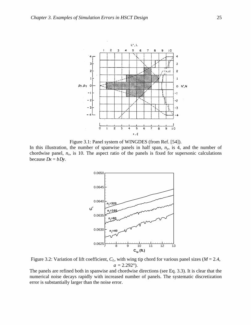
Chapter 3. Examples of Simulation Errors in HSCT Design 25
Figure 3.1: Panel system of WINGDES (from Ref. [54]).
In this illustration, the number of spanwise panels in half span, ny, is 4, and the number of chordwise panel, nx, is 10. The aspect ratio of the panels is fixed for supersonic calculations because ∆x = β∆y.
Ctip (ft.)
CL
7 8 9 10 11 12 130.0625
0.0630
0.0635
0.0640
0.0645
0.0650
ny=40
ny=80
ny=160
ny=320
Figure 3.2: Variation of lift coefficient, CL, with wing tip chord for various panel sizes (M = 2.4,
α = 2.292°). The panels are refined both in spanwise and chordwise directions (see Eq. 3.3). It is clear that the numerical noise decays rapidly with increased number of panels. The systematic discretization error is substantially larger than the noise error.

Chapter 3. Examples of Simulation Errors in HSCT Design 26
Figure 3.3: Typical FE mesh for the structural optimizations.
It shows six spar groups and thirteen skin groups for the upper surface. Each group is controlled by a design variable of the structural optimization.
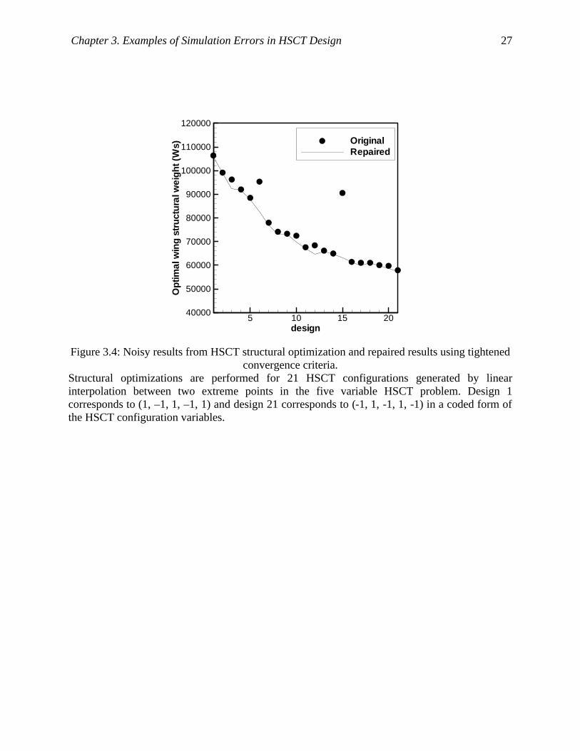
Chapter 3. Examples of Simulation Errors in HSCT Design 27
design
Opt
imal
win
gst
ruct
ural
wei
ght(
Ws)
5 10 15 2040000
50000
60000
70000
80000
90000
100000
110000
120000
OriginalRepaired
Figure 3.4: Noisy results from HSCT structural optimization and repaired results using tightened
convergence criteria. Structural optimizations are performed for 21 HSCT configurations generated by linear interpolation between two extreme points in the five variable HSCT problem. Design 1 corresponds to (1, –1, 1, –1, 1) and design 21 corresponds to (-1, 1, -1, 1, -1) in a coded form of the HSCT configuration variables.

28
Chapter 4 Response Surface Methodology
Response surface methodology (RSM) [41] is a branch of statistics used to study the
effects of independent variables on a dependent variable, called the response. Design of
experiments (DOE), analysis of variance (ANOVA), and regression analysis are the main
elements of RSM. Typically, the independent variables are assumed to be non-random and under
control of the experimenter, while the response is a random variable.
Response surface (RS) techniques have gained popularity in the application of
multidisciplinary design optimization due to their multiple merits. First, the disciplinary analysis
code is run a priori to build a database, and can be separated from the optimizer. Thus, code
integration problems due to proprietary codes are avoided by using RS approximations. Second,
the database building process is well suited for use in a parallel computing environment. Third,
the RS fit replaces the analysis code by a simple algebraic expression. Low order polynomials of
the RS fit take very little computation time compared to analysis programs such as FEA and
CFD. The RS surrogate models can be used very effectively in optimization or evaluation of
design uncertainty. Lastly, the RS fit naturally filters out the high frequency noise typical with
high-fidelity simulations.
4.1 Design of Experiments Design of experiments (DOE) provides methods to select the combinations of
independent variables for which experiments will be performed to build a database ([41], pp.79-
133). The experimenter wants to find an experimental design that is not only effective in that it
captures all important relationships between the independent and response variables, but also
efficient in that it requires a minimal number of experiments. In design optimization studies, the
response variable may be the objective function or one of the constraints, and the response
variable is modeled as a function of the design variables. The design variables are the
independent variables in the DOE and have lower and upper bounds that constitute a hypercube

Chapter 4. Response Surface Methodology 29
in which the optimum design is sought. Typically, each design variable is scaled such that it has
the range of [–1, +1] in standard DOE software to avoid numerical error in the calculation.
One natural choice for the experimental design is to use all the vertices of the hypercube
to cover all of the m-dimensional design space (m is the number of independent design
variables). It is called the full factorial design (FF) of level two (-1 and +1), to which usually a
linear polynomial model is fit. To use higher order polynomial models, the level of the
experimental design is increased. If the midpoint of each variable is added to the lower and upper
level, we have a full factorial design of level three to which a quadratic polynomial model can be
fit. One problem associated with the full factorial design is that the number of experiments
(computational simulations) increases rapidly as the number of design variables increases. In
general, the full factorial design of level l requires lm data points, or experiments. For example,
three level full factorial design for a 10 variable problem requires 310 = 59049 experiments. This
is prohibitively large unless experiments take very little time and cost. This problem is known as
the curse of dimensionality. There are alternatives to the full factorial design that require a
smaller number of points, such as face centered central composite design (FCCC) and D-optimal
design. See Appendix A for a description of the experimental designs.
Originally RS techniques have been developed to fit experimental data from agricultural
research. During the last decade, the RS techniques have gained popularity as surrogate models
for computational simulations. Certain modifications are desirable in DOE for computational
simulations. For example, use of replicates of design points is common in experimental studies,
while it is not recommended in computational simulation where the results are deterministic in
that the output (response) is the same with respect to the same input (independent variables).
However, numerical simulations can be very sensitive to nominal changes of input or may
produce different results depending on computer platforms. Therefore, it would be valid to say
that computer simulations are not perfectly deterministic.
4.2 Least Squares Fit Least squares (LS) fit is the standard way to fit a RS model equation to the data generated
by the DOE approach. In engineering applications a quadratic model is often used for the RS fit.
With n data points, the quadratic model for m independent variables is written as

Chapter 4. Response Surface Methodology 30
,,,1,1 1
0 nixxxymj mkj
ikijijkjiji K=+++= ∑ ∑≤≤ ≤≤≤
εβββ (4.1)
where yi is the i-th observation of the response variable, xji is the j-th independent variable of the
i-th observation, β’s are the model coefficients to be estimated, and εi is the random error
assumed to have zero mean and constant variance σ2. In a matrix form, the linear regression
model is
εβ += Xy (4.2)
[ ] . and
, ,
1
1
11
, where
232211211210
2
1
22
11
32
32
3222
3121
22
22
2222
2121
1
1
212
111
21
21
2212
2111
11
11
1212
1111
2
1
2
2
22
21
1
1
12
11
2
1
Tmmmm
n
i
mnmn
mimi
mm
mm
nn
ii
nn
ii
mnn
mii
m
m
nn
ii
nn
ii
mn
mi
m
m
n
i
n
i
n
i
xx
xx
xxxx
xx
xx
xxxx
xx
xx
xxxx
xx
xx
xxxx
xx
xx
xxxx
xx
xx
xxxx
x
x
xx
x
x
xx
x
x
xx
X
y
y
yy
ββββββββββ
ε
ε
εε
LLL
M
M
M
M
LM
LM
LL
M
M
M
M
M
M
LM
LM
LL
M
M
M
M
M
M
LM
LM
LL
M
M
M
M
M
M
M
M
=
=
=
=
β
εy
Note that for the quadratic model, there are p = (m+1)(m+2)/2 parameters. X is an n×p matrix of
the shape functions (monomials from the quadratic model) called the design matrix, ε is an n-
vector of noise error, and β is a p-vector of regression coefficients. For standard least squares,
estimates of the expected value of y are calculated as
,)(ˆˆ 1 yy TT XXXXX −== β (4.3)
and the residual error er is the difference between the actual data and the fit,
.yyer −= (4.4)
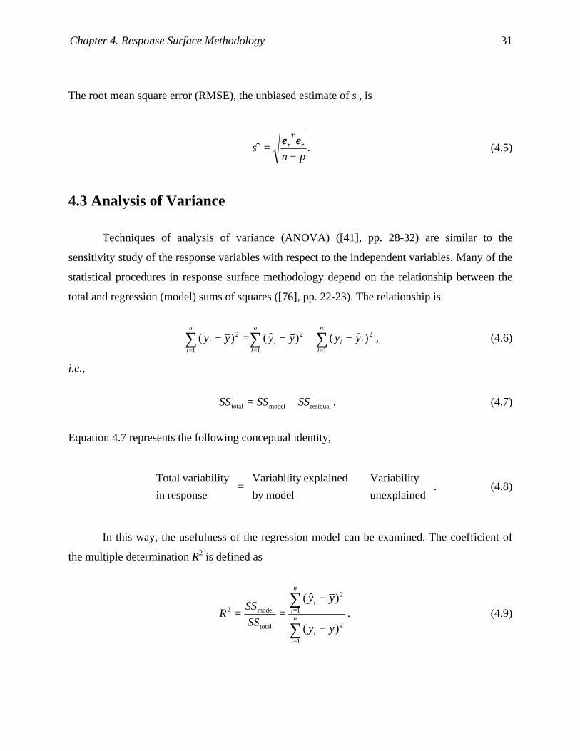
Chapter 4. Response Surface Methodology 31
The root mean square error (RMSE), the unbiased estimate of σ, is
.ˆpn
T
−= rr ee
σ (4.5)
4.3 Analysis of Variance Techniques of analysis of variance (ANOVA) ([41], pp. 28-32) are similar to the
sensitivity study of the response variables with respect to the independent variables. Many of the
statistical procedures in response surface methodology depend on the relationship between the
total and regression (model) sums of squares ([76], pp. 22-23). The relationship is
∑∑∑===
−+−=−n
iii
n
ii
n
ii yyyyyy
1
2
1
2
1
2 )ˆ()ˆ()( , (4.6)
i.e.,
residualmodeltotal SSSSSS += . (4.7)
Equation 4.7 represents the following conceptual identity,
+
=
dunexplaine
y Variabilitmodelby
explainedy Variabilitresponse in
ty variabiliTotal. (4.8)
In this way, the usefulness of the regression model can be examined. The coefficient of
the multiple determination R2 is defined as
∑
∑
=
=
−
−== n
ii
n
ii
yy
yy
SSSS
R
1
2
1
2
total
model2
)(
)ˆ(. (4.9)

Chapter 4. Response Surface Methodology 32
R2 represents the proportion of variation in the response data that is explained by the model.
From Eq. 4.6, we see that 0 ≤ R2 ≤ 1. One would expect a large value of R2 for a good RS model.
However, a large value of R2 does not necessarily imply the regression model is a good one
because adding variables to the RS model always increases R2 ([41], pp. 30-31). In addition, an
acceptable R2 value may depend on the nature of the sample data such as accuracy or
randomness ([76], pp. 37-39).
ANOVA is also the basis of the variable selection scheme. Influential variables may be
identified by analyzing the portion of the systematic variability of the response due to the change
of each independent variable. Conversely, weak variables may be identified and removed from
further analysis. A measure of the uncertainty of the regression coefficients is the partial t-test,
.)(ˆ
ˆ
1jj
T
j
XXt
−=
σ
β (4.10)
The t-statistic is essentially the ratio of the estimated coefficient to its standard error. Hence,
coefficients with small t were not accurately estimated, and they are candidates to be removed
from the model.
4.4 Noise of Simulation Data and RS Fit
Most computer simulations are deterministic unless pseudo random numbers are used. In
terms of the response surface model of Eq. 4.2, it corresponds to that the data has a negligible
random variability, i.e., ε ≈ 0. However, many computational simulation programs result in noisy
results due to discretization of continuums, truncation error, round-off error, or incomplete
convergence of iterative methods.
When the simulation data is noisy, the response surface fit is expected to smooth out the
noise and to find the true response. If the regression model (Eq. 4.2) is true, the residual error is
due to random noise error. As a result, the root mean squares error, σ , is a good estimate of the
magnitude of the noise from the simulation. When the response surface model in Eq. 4.2 is not
perfect as in many applications, RMSE is a sum of the noise error and the modeling error of the
polynomial model.

33
Chapter 5 Probabilistic Modeling of Simulation
Errors
Practices of robust design classify the design variables into control variables and random
variables [16]. The control variables are assumed to be under control of the engineers and non-
random, while the random variables have intrinsic variability. Usually the random variables are
modeled via probability distributions, and the robust design approach seeks the set of control
variables to minimize the risk due to variations of the random variables.
Sometimes simulation errors are modeled as probability distributions for deterministic
computer simulations. Probabilistic modeling of simulation errors may be based on the typical
magnitude of errors of the computational simulation [77]. It might be justified by the fact that
when one picks a design point randomly in the design space, the error is randomized due to the
random sampling. However, the probabilistic model is often used without any justification of the
model based on data, by simply assuming that the error is following a distribution such as
uniform, Gaussian, etc. For a better model of the simulation error, systematic examination of the
error characteristics is necessary.
5.1 Overview of Probabilistic Modeling of Errors
Probabilistic models are more realistic for noise error than systematic error. Once the
distribution of the simulation error is found, detailed information on the error can be obtained.
Simulation and modeling theory [61], [62] provides techniques to find the distribution of
simulation error from sample data. Our goal is to model the simulation error via probability
distribution functions. The procedure can be summarized in four steps.

Chapter 5. Probabilistic Modeling of Simulation Errors 34
Step 1: Examine the sample data
Do an exploratory examination of the sample data. Simple graphical tools such as a
histogram or box plot can be useful [78] to observe the characteristics of the error.
Possible questions are: 1) Is the error discrete or continuous? 2) Is the error systematic or
noisy? 3) Is the error symmetric about the mean? 4) What is the typical magnitude of
error? 5) Is the error homogeneous over the design space? 6) Are there any unusual data
points of extremely large error? 7) Is the Gaussian model reasonable?
Step 2: Select candidate model distributions
According to the examination of Step 1, select a few candidate distributions that seem to
fit the sample data well. In some cases, theories behind the sample data may suggest a
certain model distribution.
Step 3: Fit the model distribution to the sample data
Usually a model distribution has one or more parameters to be estimated to fix the
specific distribution from a distribution family. The model distribution is fitted to the
sample data by finding the parameters that fit the data best.
Step 4: Check how good the fit is
The fitted distribution should be compared with the data to check the quality of fit. A few
goodness-of-fit tests are available.

Chapter 5. Probabilistic Modeling of Simulation Errors 35
5.2 Model Distribution Functions
Simulation and modeling theory provides various model distribution functions to be used
as candidates for simulation errors [61], [62], [63]. Table 5.1 describes three distributions we
have considered: Gaussian, exponential, and Weibull distributions. The Gaussian distribution is a
symmetric bell shaped distribution that is very often used to model random variability. It is the
distribution behind linear theory of statistics and has many appealing theoretical properties. The
exponential and Weibull distributions are defined for nonnegative random variables and
therefore are one-sided. For certain cases, the simulation error is expected to be nonnegative, and
the one-sided model distributions are expected to work better than symmetric ones.
Model distribution functions usually have a few parameters that define the distribution.
For example, the Gaussian distribution has mean µ and standard deviation σ as parameters.
Figure 5.1 shows the probability density function (PDF) of the Gaussian distribution for different
standard deviations σ. The exponential distribution has only one free parameter β. The Weibull
distribution has two parameters, the shape parameter α, and the scale parameter β. Figure 5.2
shows the PDF of the Weibull distribution for various shape parameters α. Note that the Weibull
distribution reduces to the exponential distribution when α = 1. One common application of the
exponential and Weibull models is for modeling of time to failure [62]. See Appendix B for the
interpretation of the Weibull distribution based on the concept of failure rate.
5.3 Maximum Likelihood Estimate of Model Distribution
We use maximum likelihood estimation (MLE) ([61], pp. 188-192) to fit the distribution
to optimization error data. Let x be a random variable whose probability density function (PDF)
f(x; β) is characterized by a single parameter β. Assuming that the sampled data xi (i = 1,…, n)
are independently and identically distributed, the probability that the sample of size n consists of
values in the small intervals, xi ≤ x ≤ xi+∆x, is given by the product

Chapter 5. Probabilistic Modeling of Simulation Errors 36
.))(();();();( 21n
n xlxxfxxxfxf ∆=∆∆∆ ββββ L (5.1)
The xi ’s are fixed at the sample values, and l(β) is called the likelihood function:
( ) ( ).;1
∏=
=n
iixfl ββ (5.2)
For example, when f(x; β) is the exponential distribution function,
)exp(1
)(1 ββ
β in
i
xl −= ∏
=
. (5.3)
MLE seeks the parameter ß that maximizes the likelihood function, or equivalently its logarithm.
For example, the log likelihood function of the exponential distribution is
( ) ( ) .1
loglog1
∑=
−−=n
iixnl
ββ (5.4)
From ( )( ) ( ) 0/log =∂∂ βl , the MLE solution can be shown to be the mean of the data. However,
for more general distributions MLE may require the solution of a system of nonlinear equations.
5.4 χ2 Goodness-of-Fit Test
Once we get the MLE of the parameters, we check whether the data is consistent with our
trial distribution with the χ2 (Chi-square) goodness-of-fit test ([61], pp. 192-198). To compute
the χ2 test statistic, we subdivide the entire range of the fitted distribution into k adjacent
intervals. For sample size n, the test statistic is calculated as

Chapter 5. Probabilistic Modeling of Simulation Errors 37
∑=
−=
k
j j
jj
np
npN
1
22 ,
)(χ (5.5)
where Nj is the observed frequency in the j-th interval. pj is the expected probability of the j-th
interval from the fitted distribution, and then npj is the expected frequency in the j-th interval. If
the fit is good, (Nj - npj) will be small, and the test statistic χ2 will also be small. Therefore, a
large value of the χ2statistic indicates that the data is inconsistent with the fitted distribution. The
largeness of the test statistic is usually measured by comparing it to the χ2distribution with (k-1-
m) degrees of freedom (m is the number of parameters in the distribution) to which it will belong
as n goes to infinity. This comparison is given in terms of a p-value, which is defined as the
probability that the test statistic is greater than the calculated value when the fitted distribution is
true. A p-value near one implies a good fit and a small chance that the data is inconsistent with
the distribution. Conversely, a small p-value implies a poor fit and a high chance that the data is
inconsistent with the distribution.
5.5 Probability Plot
For a sample of size n, xi (i = 1, …, n), an approximate cumulative distribution function
can be constructed. First, the sample data is sorted in ascending order and x(i) denotes the i-th
smallest data. Since the cumulative distribution function (CDF) F(x(i)) is defined as Prob(x ≤ x(i)),
the empirical cumulative distribution function (ECDF) ([61], pp.181-183) is expressed as
Fn(x(i)) = i/n. (5.6)
Obviously, i/n is an estimate of Prob(x ≤ x(i)) from the sample data. It is known that Fn(x(i))
converges to the CDF F(x) from which the xi’s are taken as the sample size increases to infinity.
In practice, a slight modification is done for Eq. 5.6 to avoid the problem of making Fn = 1 for a
finite x(n),
Fn(x(i)) = (i-0.5)/n. (5.7)

Chapter 5. Probabilistic Modeling of Simulation Errors 38
The probability plot ([61], pp. 181-188) compares the ECDF of a sample with the CDF of
an assumed distribution. There are several kinds of probability plots. Here we discuss only one
type, called a Quantile-Quantile plot (Q-Q plot). A quantile of order q is defined as F-1(q), where
F-1 is the inverse function of CDF F(x); it is the value of x for which the cumulative density of x
is q. For a Q-Q plot, the following n points are plotted,
(F-1((i-0.5)/n), x(i)) (i = 1,…,n), (5.8)
which are pairs of the quantile of CDF and the corresponding quantile ECDF. If the assumed
CDF is true, we expect that the pairs of the quantiles are the same for a large sample. Therefore,
when we compare the sample data and the fitted distribution via MLE, we expect that the Q-Q
plot will be close to a straight line of unit slope passing the origin if the fit is good. Any
systematic deviation from the reference line indicates that the fit is not good.
5.6 Indirect Fit of Error Distribution using Differences of
Simulation Results
Our objective is to find a probability distribution of error from a lower fidelity
simulation. When MLE (see Section 5.3) is used to fit the error distribution, it is usually
necessary to run higher fidelity runs to estimate the error of the lower fidelity runs. However, the
high-fidelity method may be too expensive computationally, or sometimes high-fidelity
simulations are not available. In these situations, we may be able to find the error distributions by
fitting the differences between two results from different sets of program control parameters.
Examples of program control parameters can be convergence criteria of iterative methods or
initial design points in optimization.
Assume that we have simulation results with two different sets of program control
parameters. We denote the simulation results by y1 and y2 according to the program control
settings used. The unknown true solution is common for y1 and y2, and will be denoted by yt.

Chapter 5. Probabilistic Modeling of Simulation Errors 39
Then the simulation errors with control parameters setting #1 and setting # 2 can be represented
as random variables, s and t, respectively:
.
,
2
1
t
t
yyt
yys
−=−=
(5.9)
For example, if the error data follows the exponential distribution, s and t have the
following probability distribution functions
).exp(1
)(
),exp(1
)(
22
11
ββ
ββt
th
ssg
−=
−= (5.10)
The difference between the pair of y1 and y2 is equal to the difference between the errors, because
the true solution yt is the same. That is,
x = s - t = (y1 - yt) - (y2- yt) = y1 - y2. (5.11)
The probability density of the differences of simulation results (in short, simulation differences)
can be obtained as a convolution of the joint distribution [79] of g(s) and h(t), provided that s and
t are independent each other:
.
0)exp(1
)()(
0)exp(1
)()(
),;(
121
2210
21
≥−+
=−
<+
=−
=
∫
∫
∞
∞
xifx
dsxshsg
xifx
dsxshsg
xf
x βββ
βββββ (5.12)
This is a continuous distribution of the simulation difference x ∈ (-∞, ∞). Now we can fit the
simulation difference, x, to the model function Eq. 5.12 via MLE. In the maximum likelihood
approach we find parameters β1 and β2 that maximize the likelihood function

Chapter 5. Probabilistic Modeling of Simulation Errors 40
( ) ( ),,;,1
2121 ∏=
=n
iixfl ββββ (5.13)
where f is defined in Eq. 5.12. This is an unconstrained optimization problem in two variables.
Equivalently we can maximize the log likelihood function,
( ) ( ).,;log,log1
2121 ∑=
=n
iixfl ββββ (5.14)

Chapter 5. Probabilistic Modeling of Simulation Errors 41
Table 5.1: Examples of model functions for continuous distribution. Gaussian Exponential Weibull
Density f(x)
( )
−−2
2
2 2exp
2
1σ
µ
πσ
x
≥
−
otherwise
xifx
0
0exp1
ββ
≥
−−−
otherwise
xifx
x
0
0exp1
α
αα
βαβ
Parameters Location parameter µ Scale parameter σ
Scale parameter β Shape parameter α Scale parameter β
Mean µ β
Γ
ααβ 1
Variance σ2 β2
Γ−
Γ
22 1122
ααααβ

Chapter 5. Probabilistic Modeling of Simulation Errors 42
x
f(x)
-5 -4 -3 -2 -1 0 1 2 3 4 50.0
0.2
0.4
0.6
0.8
1.0
1.2
σ=0.5, µ=0σ=1.0, µ=0σ=1.5, µ=0σ=2.0, µ=0
Figure 5.1: Probability density functions for Gaussian with µ = 0 and various σ.
x
f(x)
0 1 2 3 4 50.0
1.0
2.0
3.0
α = 0.5, β = 1α = 1.0, β = 1α = 2.0, β = 1α = 4.0, β = 1
Figure 5.2: Probability density functions for Weibull with β = 1 and various α.

43
Chapter 6 Robust Regression Techniques and
Outlier Detection
The least squares fit in standard response surface methodology is not robust. If the
database for the response surface fit contains simulation results with large errors, the least
squares fit can be greatly affected by the bad data points. The objective of robust statistics [64],
[65] is to provide alternative estimation techniques when standard assumptions for the model are
not valid. For example, in multiple linear regression, the random error is assumed to have a
constant variance with zero mean. Robust regression techniques are designed to give a
reasonable fit when the error distribution is not homogeneous, and give estimates as good as the
least squares fit when the error distribution is ideal. Also, robust regression techniques provide
protection against outliers [43], [65], data points out of the main trend. It gives a robust fit for the
data contaminated with outliers (bad simulation results) and enables us to identify those outliers,
which may lead to further investigation of the cause of the error.
6.1 Iteratively Reweighted Least Squares
Among several robust regression methods we will discuss the M-estimator (maximum
likelihood type) [64], [65]. It can be shown that the MLE is an M-estimator. For a more robust
estimate of ß, we minimize a measure of the residuals ri:
.)ˆ(
where,)()ˆ(1 s
Xrre i
i
n
ii
ββ
−== ∑
=
yρ (6.1)
Here, ρ is a function of the residual scaled by s, a known estimate of the standard deviation of ε.
For example, in the case of the familiar least squares method, ρ(ξ) = ξ 2/2. A necessary condition
for a minimum is

Chapter 6. Robust Regression Techniques and Outlier Detection 44
0)ˆ( =∇ βe . (6.2)
The ψ function is defined as the derivative of ρ
.)(
)(ξξρ
ξψd
d= (6.3)
Then, a necessary condition for a minimum becomes
T
nT
nT rrrX ))(),...,(),((),...,,( where,0 2121 ψψψψψψ === ψψ . (6.4)
To write Eq. 6.4 in a form of weighted least squares, we define the weighting function as
.)(
)(ξξψ
ξ =w (6.5)
Now, with r = (r1, …, rn)T, Eq. 6.4 becomes
)).(...,),(),(()( where,0)( 21 nT rwrwrwdiagWWX == rrr (6.6)
Note that for ordinary least squares ψ(ξ) = ξ and w(ξ) = 1.
For ordinary least squares, Eq. 6.6 is a linear equation for the coefficient vector β
through the scaled residual r. However, in general Eq. 6.6 is a system of nonlinear equations, and
iterative methods are required to obtain the solution. The most popular approach is iteratively
reweighted least squares (IRLS), which is attributed to Beaton and Tukey [66]. Using the
definition of residual in Eq. 6.1, the necessary condition of Eq. 6.6 is written as
,)(ˆ)( yrr WXXWX TT =β (6.7)
which can be expressed as an iterative formula

Chapter 6. Robust Regression Techniques and Outlier Detection 45
,ˆˆ
ˆ)(
1)(
)1( yyy
−
−=
−
+
sX
WXXsX
WXi
Ti
Ti βββ (6.8)
or
).ˆ(ˆˆ
ˆˆ )()(
1)(
)()1( ii
Ti
Tii XsX
WXXsX
WX βββ
ββ −
−
−+=
−
+ yyy
(6.9)
Several possible weighting functions summarized in Table 6.1 and Figure 6.1, were
considered here. We preferred Beaton and Tukey’s biweight function [66] to Huber’s minimax
[80] because it gives zero weighting to the outliers and thus the outliers are distinctly identified
(see Figure 6.1). s is calculated as |)ˆ(|5.1 iiXmedian β−y as recommended by Myers [76]. The
other function in Table 6.1, labeled as NIRLS, will be discussed later in Section 6.2. B in Table
6.1 is a tuning constant depending on the characteristics of the error distribution. Myers [76]
suggested limiting the tuning constant to a range of one to three. The shape of the weighting
functions in Figure 6.1 clearly shows that they penalize outliers with zero or low weighting while
giving a weighting of one or near one to inliers.
Equation 6.9 is not guaranteed to converge to the global minimum of e( β ). Because the
IRLS results depend on the initial guess for the regressor coefficients, β , we need a good initial
guess of β . With a non-redescending ψ function (Figure 6.2) like Huber’s minimax, Birch [81]
proved that Eq. 6.9 is globally convergent to a unique solution, the global minimum of e( β ).
Therefore, to get the initial estimates of the regressor coefficients β , we adopted Huber’s
minimax function. Then the IRLS procedure using the biweight function was continued using
these initial coefficients. The IRLS procedure with Huber’s minimax function converged faster;
it took about 20 iterations for convergence while using the biweight required about 100 iterations
for the data from structural optimization of the HSCT.
The IRLS procedure is demonstrated for a one-dimensional example in Figure 6.3. The
eleven data points were generated by adding some artificial errors to the true response of y = 0.8
- 0.7x + 0.25x2. Two data points at x = 0.5 and 0.9 have particularly large errors and may be

Chapter 6. Robust Regression Techniques and Outlier Detection 46
called outliers. The least squares fit is distracted by the outliers and over-predicts the response.
Robust regression techniques are expected to give a better fit than the least squares fit. The IRLS
procedure using the biweight function is applied. The IRLS fit is seen to give a better prediction
by giving zero weighting and effectively excluding the outliers from the fit. Note that outliers are
identified by the IRLS procedure. In practice, we may want to investigate the cause of the
outliers and efforts to repair them may be desirable.
6.2 Nonsymmetric IRLS (NIRLS)
Now we consider the NIRLS entry in Table 6.1. The usual IRLS procedure assumes
symmetry of the error with zero mean error. However, for optimization data, the scaled residual
ri is mostly positive for outliers (see Eq. 6.1), because they are caused by the failure of the
optimization while seeking a minimum. For unconstrained optimization, any failure of
optimization procedure will produce an optimum with one-sided error. Also, some of constrained
optimization algorithms seek the optimum in feasible region, and premature convergence of
optimization will produce one-sided error except that the optimizer cannot find a feasible design.
To account for the skewed error in the outliers, we devised a nonsymmetric weighting
function by combining the biweight and Huber’s weighting function, and labeled it as the NIRLS
(nonsymmetric IRLS) weighting function. For the NIRLS weighting function shown in Figure
6.1, data points with negative residuals are down-weighted according to Huber’s function,
whereas points with positive residuals are down-weighted by the biweight function. In this way,
NIRLS down-weights points with positive residual error more severely. NIRLS has been
successfully applied to noisy data from structural optimization of the HSCT [47], and to low
fidelity optimization data of cracked composite panels [82]. We will demonstrate the advantage
of the nonsymmetric weighting function on the Rosenbrock test problem in Chapter 8 and
structural optimization of the HSCT in Chapter 10.
IRLS/NIRLS techniques effectively remove outliers from the fit by downweighting them.
However, when only a few data points are used in a response surface fit due to consideration of
computational cost, excluding outliers may be undesirable because it may lead to poor
predictions where the outliers are located. Therefore, a better strategy is to repair the detected
outliers by performing higher fidelity simulation runs if practical [46]. If the high-fidelity runs

Chapter 6. Robust Regression Techniques and Outlier Detection 47
are much more expensive than the lower fidelity runs, repairing only the outliers detected by
IRLS/NIRLS may have a computational advantage over performing high-fidelity runs for all the
runs. The general IRLS/NIRLS procedure described in this section is summarized in Figure 6.4.

Chapter 6. Robust Regression Techniques and Outlier Detection 48
Table 6.1: Weighting functions of M-estimator. Name W(r) Range Tuning Constant
Huber’s minimax [80] 1
H r -1
r ≤ H
r > H H = 1.0
Beaton and Tukey’s
biweight [66]
(1-(r/B)2)2
0
r ≤ B
r > B B = 1.0 or 1.9
NIRLS
H r -1
1
(1-(r/B)2)2
0
r ≤ -H
-H < r ≤ 0
0 < r ≤ B
r > B
H = 1.0
B = 1.0 or 1.9

Chapter 6. Robust Regression Techniques and Outlier Detection 49
Residual, r
Wei
ghtin
g,w
(r)
-4 -2 0 2 40.0
0.2
0.4
0.6
0.8
1.0
1.2
1.4
1.6HuberBiweightNIRLS
Figure 6.1: Various weighting functions of the M-estimator.
Residual, r
ψ(r
)
-4 -2 0 2 4-1.5
-1.0
-0.5
0.0
0.5
1.0
1.5
2.0HuberBiweightNIRLS
Figure 6.2: The corresponding ψ functions of the M-estimator.
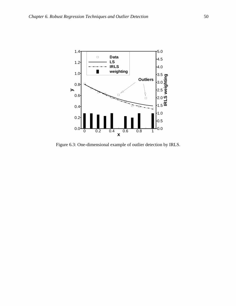
Chapter 6. Robust Regression Techniques and Outlier Detection 50
x
y
IRLS
wei
ghtin
g
0 0.2 0.4 0.6 0.8 10.0
0.2
0.4
0.6
0.8
1.0
1.2
1.4
0.0
0.5
1.0
1.5
2.0
2.5
3.0
3.5
4.0
4.5
5.0DataLSIRLSweighting
Outliers
Figure 6.3: One-dimensional example of outlier detection by IRLS.

Chapter 6. Robust Regression Techniques and Outlier Detection 51
Get initial regression coefficients using Huber’s weighting function
IRLS or NIRLS fit
Identify outliers with very small weighting
Repair outliers using high fidelity optimizations
Least squares fit with the repaired data
Is high fidelity optimization available?
Improved response surface fit
Examine the outliers to find the cause of error
Data from low fidelity optimization runs
No
Use the IRLS orNIRLS fit
Yes
Figure 6.4: Flow chart of the IRLS/NIRLS procedure for low fidelity optimization data.

52
Chapter 7 RS Modeling of Errors from
Supersonic Aerodynamic Simulation
Discretization error is fundamental to all simulations using a discretized representation of
a continuum. In Section 3.1, we observed that the CL calculation from WINGDES had a
systematic discretization error and low amplitude noise as well. It was seen that the noise error
was small compared to the discretization error. Traditionally, Richardson extrapolation is used to
get accurate estimates of the continuum solution from results on relatively coarse meshes. One
important aspect of Richardson extrapolation is that it applies not only to solution values at mesh
points, but also to a solution functional such as CL. However, Richardson extrapolation tends to
magnify noise errors such as machine round-off errors and incomplete iteration errors (Ref. [9],
p. 109-112).
Alvin [37] applied response surface (RS) techniques to model the discretization error by
incorporating mesh size, h, into the RS model. He showed that the RS approach effectively
reduced discretization error in a finite element analysis of a one-dimensional bar, and it was
noted that the RS model had computational advantage via careful use of design of experiments.
Kammer et al. [38] used a rational polynomial function as a RS model to improve extrapolation
results when coarser mesh results are used. We utilize their RS approaches to model the
discretization error from WINGDES, and the RS approach will be compared to Richardson
extrapolation. The results demonstrate again the computational advantages of the RS model for
discretization error. Besides, we address several new aspects of the RS approach. First, we
perform a grid convergence study for WINGDES to estimate the order of the discretization error.
Second, the noise filtering capability of a RS fit may have an additional advantage over
Richardson extrapolation. Third, an approach of fitting a RS model to the Richardson
extrapolation results will be compared to the RS approach in terms of accuracy and
computational cost.

Chapter 7. RS Modeling of Errors from Supersonic Aerodynamic Simulation 53
7.1 Grid Convergence Study of WINGDES
Figure 7.1 shows the grid convergence of CL from WINGDES for the reference HSCT
configuration in the five design variable problem. Originally, the number of spanwise panels in
the half span, ny, was 40. The reciprocal of ny is a measure of the mesh step size, h. Here we
changed panel sizes widely, from a very coarse panel system of ny = 10, to 320 by increments of
10. The panels are refined in both spanwise and chordwise directions such that the number of
chordwise panels, nx, is proportional to ny (see Eq. 3.3). The circle symbols in Figure 7.1
correspond to mesh halving cases, that is ny = 10, 20, 40, 80, 160, and 320. It is seen that the
discretization error would be no greater than 0.002 for ny = 40, about 3% of CL. Because the
theoretical convergence property of the supersonic panel method is not known, the order of error
convergence should be estimated from the simulation results. In Richardson extrapolation, the
discretized simulation is assumed to have error terms expressed in a polynomial of a step size h,
)( 1+++= qqh hOhyy α , (7.1)
where yh is the discretized solution for the current value of h, y is the continuum solution, α is an
unknown coefficient, and q is the order of the method [38]. Asymptotic error convergence is
achieved when the higher order error term, O(hq+1), is small enough compared to the leading
error term, αhq, and α does not change with h.
If the error of yh is first order, i.e., q = 1, the response of yh according to step size, h,
should be linear. Figure 7.1 indicates that the order of error convergence q is lower than one for
CL from WINGDES because the slope of the grid convergence curve gets steeper as the mesh
step size decreases. It is not unusual that low order panel methods show slow error convergence
[83], [84]. If simulation results from three different step sizes are available, the order of
convergence q can be estimated (Ref. [9], p. 131). If the mesh is refined by reducing the mesh
size by half, using Eq. 7.1
qqq
hh
hh
hhhh
yyyy
r 2)4/()2/(
)2/(
4/2/
2/ =−
−=
−−
= . (7.2)

Chapter 7. RS Modeling of Errors from Supersonic Aerodynamic Simulation 54
Therefore,
)2log(/)log(rq = . (7.3)
Table 7.1 shows estimates of q using three WINGDES results of mesh halving. It appears that
asymptotic convergence is achieved after ny = 40 with q ≈ 0.5, and the error converges like h0.5.
7.2 Higher Order Formulas using Richardson Extrapolation
7.2.1 Extrapolation for h = 0
Richardson extrapolation generates higher order formulas from a series of relatively
coarse mesh results (Ref. [57], pp. 180-186). Numerical results of O(hq) can be expressed as,
yh = y + α1 hq + H.O.T., (7.4)
where H.O.T. represents higher order terms than hq. Note that the second leading error term is
not necessarily hq+1 for CL from WINGDES because q is a non-integral number. If the mesh is
refined by reducing the step size by half, i.e., mesh-halving,
yh/2 = y + α1 (h/2)q +H.O.T., (7.5)
yh/4 = y + α1 (h/4)q +H.O.T.. (7.6)
A higher order formula is obtained by eliminating the leading error term, α1 hq. By subtracting 2q
times Eq. 7.5 from Eq. 7.4,
12
2 2/)2(
−−
= qhh
q
h
yyy , (7.7)

Chapter 7. RS Modeling of Errors from Supersonic Aerodynamic Simulation 55
where the superscript number in the parenthesis indicates that the order of the formula is higher
than hq. By the same token, from Eq. 7.5 and Eq. 7.6,
12
2 2/4/)2(2/ −
−= q
hhq
h
yyy . (7.8)
Richardson extrapolation assumes that the errors are in the asymptotic convergence
range. Caution should be taken because Richardson extrapolation will be inaccurate if the mesh
step size is not small enough for the error to reach asymptotic convergence. Moreover, noise in
data, typical in numerical simulations on discretized models, tends to be magnified by
extrapolation (Ref. [9], p. 109-112).
7.2.2 Extrapolation for Finite Mesh Sizes
Richardson extrapolation is designed to extrapolate for y, the continuum solution. In
practice, the continuum solutions are not known or are not calculable due to excessive
computational cost. That makes it difficult to compare the accuracy of the extrapolation. For
quantitative comparison of accuracy of extrapolation, Richardson extrapolation may be
reformulated to predict results for finer, but still finite meshes.
By solving Eq. 7.4 and Eq. 7.5 for y and α1, and substituting them into Eq. 7.6, we obtain
a higher order formula for h/4,
+−
−−
++
= qqhhhh
h q
yyyyy
21
121
2
12/112 2
2/2/)2()4/( . (7.9)
Note that a parenthesis is used in the subscript of y(h/4)(2) to indicate an extrapolation for a finitely
refined mesh. To get an extrapolation for h/8, we need
yh/8 = y + α1 (h/8)q + H.O.T.. (7.10)
Chapter 7. RS Modeling of Errors from Supersonic Aerodynamic Simulation 56
By solving Eq. 7.5 and Eq. 7.6 for y and α1, and substituting them into Eq. 7.10, a higher order
formula similar to Eq. 7.9 is obtained,
+−
−−
++
= qqhhhh
h q
yyyyhhy
21
121
21
2/112)4/,2/(
2
4/2/4/2/)2()8/( , (7.11)
where (h/2, h/4) in the left hand side indicates that it is a higher order formula using solutions at
h/2 and h/4. To get a higher order formula for h/8 using solutions at h and h/2, Eqs. 7.4, 7.5, and
7.10 are combined,
+−
−−
++
= qqhhhh
h q
yyyyhhy
21
121
2
12/112
)2/,(3
2/2/)2()8/( . (7.12)
7.3 RS Modeling of Discretization Error
A RS model is built for pre-defined ranges of design variables, forming the design box.
Typically, the design box encloses regions of interest, and the RS model is used to predict the
response within the design box. On the other hand, prediction outside of the design box is not
recommended because such extrapolation using a RS model may have a large error. Richardson
extrapolation is used to predict the continuum solution because of the unaffordable cost of the
discretized solution for very fine meshes. To apply Richardson extrapolation, asymptotic
convergence of the error needs to be achieved, and the order of error should be known. If similar
conditions are met, RS models can be used to extrapolate for the continuum solution.
Experiments are performed on a few different mesh sizes, h, which are incorporated into
a RS model. One possible advantage of the RS approach lies in its flexibility in selection of data
points. A carefully designed experiment may use solutions of refined meshes only sparingly,
while Richardson extrapolation requires a series of solutions at different mesh sizes for every
design point.

Chapter 7. RS Modeling of Errors from Supersonic Aerodynamic Simulation 57
7.3.1 Incorporating Discretization Error into the RS Model
The RS approach is applied to a one-dimensional problem: CL from WINGDES for
different wing tip chords (ctip). Following Ref. [38], a polynomial model, quadratic in x and order
q in h, is proposed,
,2321
2210 εαααβββ ++++++= qqq
h hxxhhxxy (7.13)
where yh is the discretized solution of CL, ε is a random error, and the α’s and β’s are coefficients
to be estimated. Linear interaction terms between h and x are included and the order of error
estimated in Section 7.1, q = 0.5, was used in the model. Note that the continuum solution may
be obtained by setting h = 0,
2
2100 xxyy h βββ ++== = . (7.14)
7.3.2 Comparison between Richardson Extrapolation and RS Approach
Richardson extrapolation (RE) was used to predict continuum solutions of CL. Two cases
of mesh fineness were tried as follows.
• RE1: Richardson extrapolation from h, h/2 (ny = 40, 80) using Eq. 7.7
• RE2: Richardson extrapolation from h/2, h/4 (ny = 80, 160) using Eq. 7.8
For each case, RE is applied to CL for six HSCT designs of different ctip. Since a coarser mesh
result and a finer mesh result are required to perform a Richardson extrapolation, there are
twelve WINGDES runs for each case, six on coarser mesh and six on finer mesh (see Figure
7.2). Next, the RS model (Eq. 7.13) was fit to each of the two experimental designs with the
twelve data points used in RE approach. In addition, two experimental designs of less number of
refined mesh results were tried to show computational advantages of the RS approach.
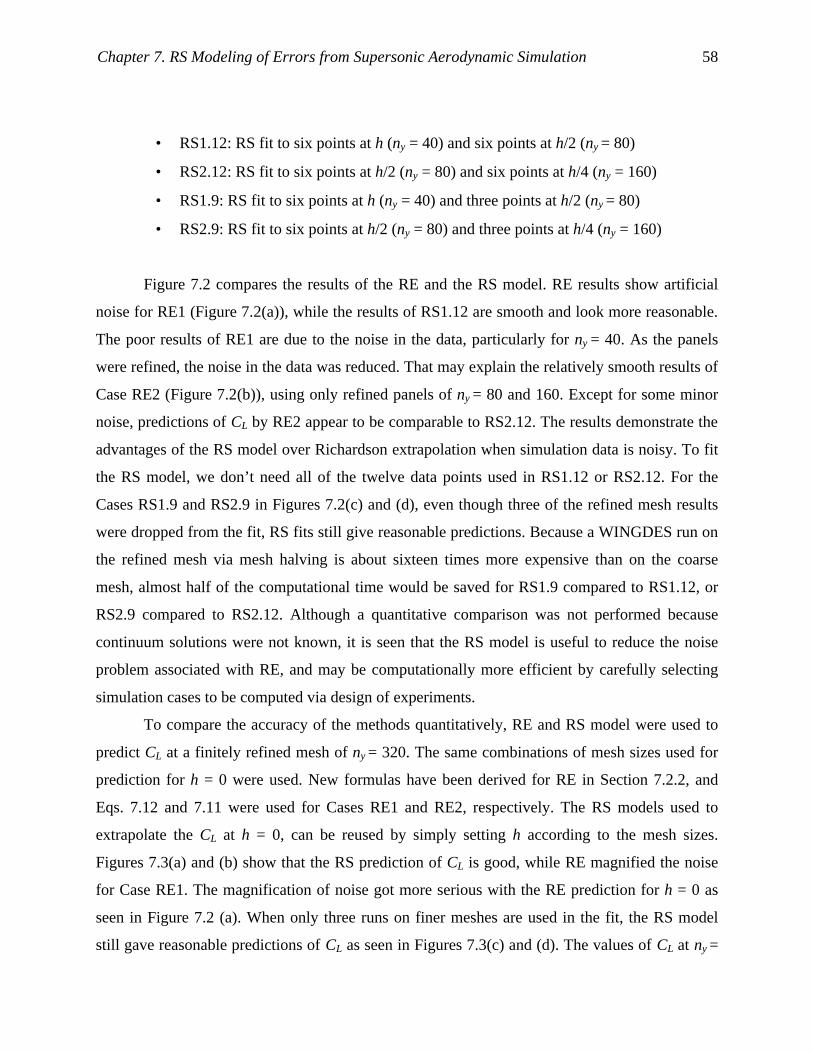
Chapter 7. RS Modeling of Errors from Supersonic Aerodynamic Simulation 58
• RS1.12: RS fit to six points at h (ny = 40) and six points at h/2 (ny = 80)
• RS2.12: RS fit to six points at h/2 (ny = 80) and six points at h/4 (ny = 160)
• RS1.9: RS fit to six points at h (ny = 40) and three points at h/2 (ny = 80)
• RS2.9: RS fit to six points at h/2 (ny = 80) and three points at h/4 (ny = 160)
Figure 7.2 compares the results of the RE and the RS model. RE results show artificial
noise for RE1 (Figure 7.2(a)), while the results of RS1.12 are smooth and look more reasonable.
The poor results of RE1 are due to the noise in the data, particularly for ny = 40. As the panels
were refined, the noise in the data was reduced. That may explain the relatively smooth results of
Case RE2 (Figure 7.2(b)), using only refined panels of ny = 80 and 160. Except for some minor
noise, predictions of CL by RE2 appear to be comparable to RS2.12. The results demonstrate the
advantages of the RS model over Richardson extrapolation when simulation data is noisy. To fit
the RS model, we don’t need all of the twelve data points used in RS1.12 or RS2.12. For the
Cases RS1.9 and RS2.9 in Figures 7.2(c) and (d), even though three of the refined mesh results
were dropped from the fit, RS fits still give reasonable predictions. Because a WINGDES run on
the refined mesh via mesh halving is about sixteen times more expensive than on the coarse
mesh, almost half of the computational time would be saved for RS1.9 compared to RS1.12, or
RS2.9 compared to RS2.12. Although a quantitative comparison was not performed because
continuum solutions were not known, it is seen that the RS model is useful to reduce the noise
problem associated with RE, and may be computationally more efficient by carefully selecting
simulation cases to be computed via design of experiments.
To compare the accuracy of the methods quantitatively, RE and RS model were used to
predict CL at a finitely refined mesh of ny = 320. The same combinations of mesh sizes used for
prediction for h = 0 were used. New formulas have been derived for RE in Section 7.2.2, and
Eqs. 7.12 and 7.11 were used for Cases RE1 and RE2, respectively. The RS models used to
extrapolate the CL at h = 0, can be reused by simply setting h according to the mesh sizes.
Figures 7.3(a) and (b) show that the RS prediction of CL is good, while RE magnified the noise
for Case RE1. The magnification of noise got more serious with the RE prediction for h = 0 as
seen in Figure 7.2 (a). When only three runs on finer meshes are used in the fit, the RS model
still gave reasonable predictions of CL as seen in Figures 7.3(c) and (d). The values of CL at ny =

Chapter 7. RS Modeling of Errors from Supersonic Aerodynamic Simulation 59
320 from WINGDES are listed in Table 7.2 along with the errors of RE, defined as CL (predicted
by RE) – CL (data from WINGDES). RE1 had an average error of 5.052×10⁻⁵ due to the noise,
while the average error of RE2 was only 1.555×10⁻⁵.
Table 7.3 shows the errors in CL predictions by the RS model. The average error of
RS1.12, 3.178×10⁻⁵, is substantially lower than that of RE1, 5.052×10⁻⁵. Note that the average
error of RS1.9, 4.854×10⁻⁵, was lower than that of RE1, although only nine data points were used
in the RS fit; the RS approach was better than RE in terms of both accuracy and efficiency, when
the noisy data of ny = 40 was used in calculation. When the data is less noisy, RE and RS showed
comparable average errors: 1.555×10⁻⁵ for RE2 and 1.532×10⁻⁵ for RS2.12. With fewer data
points used in the fit, RS2.9 showed a higher average error of 2.543×10⁻⁵ than RE2. However,
the loss of accuracy of the RS fits due to removing a few runs on finer meshes, is small in terms
of the magnitude of the discretization errors seen in Figure 7.3.
7.3.3 RS Fit to the Data from Richardson Extrapolation
There might be a question concerning the RS approach; is the RS model of Eq. 7.13
necessary? Alternatively, a simpler RS model may be fit to the Richardson extrapolation results,
εβββ +++= 22108/ xxyh . (7.15)
This posterior RS approach will be denoted RSRE, and it is applied to the results of RE1 and
RE2.
• RSRE1: RS fit to RE results for h/8 (ny = 320) from h, h/2 (ny = 40, 80)
• RSRE2: RS fit to RE results for h/8 (ny = 320) from h/2, h/4 (ny = 80, 160)
Figure 7.4 compares the results of RS and RSRE. From Figures 7.4(a) and (b), we
observe that RSRE1 and RSRE2 give almost the same results as RS1.12 and RS2.12,
respectively. It is seen that the mean errors of RS1.12 and RS2.12 in Table 7.3 are the same as
those of RSRE in Table 7.4, up to four significant figures. This is a little bit surprising for

Chapter 7. RS Modeling of Errors from Supersonic Aerodynamic Simulation 60
RS1.12 where RS produced a smooth response in contrast to the noise in the RE results. That
should be attributed to the fact that only two levels of h were used in the experimental designs.
With only two levels of h, the RS fit does no noise filtering in h. In other words, the smooth RS
results of RS1.12 were thanks to noise filtering in x, which can be fully achieved when fitting a
RS model to RE data. If more levels of h are used in the fit, it is possible that the RS approach
will have noise filtering in h, showing some advantage over RSRE. However, the RS approach
still may have some computational advantage over the RSRE approach for which point-by-point
RE should be performed beforehand. Figures 7.4(c) and (d) show that RS1.9 and RS2.9 give a
reasonable CL prediction comparable to the RSRE approach, although three of the finer mesh
results were not used in the fit.

Chapter 7. RS Modeling of Errors from Supersonic Aerodynamic Simulation 61
Table 7.1: Estimates of order of error convergence of CL from WINGDES. r q
ny = 10, 20, 40 2.1459 1.102
ny = 20, 40, 80 0.7097 -0.495
ny = 40, 80, 160 1.4329 0.519
ny = 80, 160, 320 1.3557 0.439

Chapter 7. RS Modeling of Errors from Supersonic Aerodynamic Simulation 62
Table 7.2: Error in CL (ny = 320) prediction of the Richardson extrapolation. RE1 used Eq. 7.12 and RE2 used Eq. 7.11.
Error in CL (ny = 320) prediction Ctip (ft.)
CL (ny = 320) Case RE1
(Using ny = 40, 80) Case RE2
(Using ny = 80, 160) 7.0 0.0637429 -5.610×10⁻⁶ 1.084×10⁻⁵ 8.2 0.0638953 -2.859×10⁻⁶ 7.292×10⁻⁶ 9.4 0.0640406 3.033×10⁻⁵ -3.040×10⁻⁵ 10.6 0.0641707 -9.627×10⁻⁵ -2.463×10⁻⁵ 11.8 0.0643036 2.947×10⁻⁵ -4.712×10⁻⁶ 13.0 0.0644306 -1.386×10⁻⁴ 1.543×10⁻⁵
Average error 5.052×10⁻⁵ 1.555×10⁻⁵
Table 7.3: Error in CL (ny = 320) prediction of the RS model. RS model of Eq. 7.13 is used.
Error in CL (ny=320) prediction Ctip (ft.)
CL (ny = 320) Case RS1.12
(6 points in ny = 40 and 6 points
in ny = 80)
Case RS1.9 (6 points in ny = 40 and 3 points
in ny = 80)
Case RS2.12 (6 points in ny = 80 and 6 points
in ny = 160)
Case RS2.9 (6 points in ny = 80 and 3 points
in ny = 160) 7.0 0.0637429 -8.287×10⁻⁶ -2.755×10⁻⁵ 1.842×10⁻⁵ 5.308×10⁻⁵ 8.2 0.0638953 3.560×10⁻⁶ -2.205×10⁻⁵ -9.580×10⁻⁶ -9.128×10⁻⁷ 9.4 0.0640406 -1.021×10⁻⁶ -2.782×10⁻⁵ -2.427×10⁻⁵ -3.195×10⁻⁵ 10.6 0.0641707 -1.395×10⁻⁵ -3.680×10⁻⁵ -1.757×10⁻⁵ -3.195×10⁻⁵ 11.8 0.0643036 -5.340×10⁻⁵ -6.712×10⁻⁵ -7.639×10⁻⁶ -1.908×10⁻⁵ 13.0 0.0644306 -1.104×10⁻⁴ -1.099×10⁻⁴ 1.445×10⁻⁵ 1.560×10⁻⁵
Average error 3.178×10⁻⁵ 4.854×10⁻⁵ 1.532×10⁻⁵ 2.543×10⁻⁵
Table 7.4: Error in CL (ny = 320) prediction of the RS fit to the Richardson extrapolation results. RS model of Eq. 7.15 is used. RSRE1 is RS fit to RE1 of Eq. 7.12, and RSRE2 is RS fit to RE2 of Eq. 7.11.
Error in CL (ny = 320) prediction Ctip (ft.)
CL (ny = 320) Case RSRE1
(Using ny = 40, 80) Case RSRE2
(Using ny = 80, 160) 7.0 0.0637429 8.275×10⁻⁶ -1.838×10⁻⁵ 8.2 0.0638953 -3.598×10⁻⁶ 9.573×10⁻⁶ 9.4 0.0640406 1.011×10⁻⁶ 2.428×10⁻⁵ 10.6 0.0641707 1.400×10⁻⁵ 1.763×10⁻⁵ 11.8 0.0643036 5.338×10⁻⁵ 7.627×10⁻⁶ 13.0 0.0644306 1.104×10⁻⁴ -1.442×10⁻⁵
Average error 3.178×10⁻⁵ 1.532×10⁻⁵

Chapter 7. RS Modeling of Errors from Supersonic Aerodynamic Simulation 63
1/ny
CL
0.000 0.025 0.050 0.075 0.1000.061
0.062
0.063
0.064
0.065
0.066
ny=10
ny=20ny=40
ny=80
ny=320ny=160
Figure 7.1: Grid convergence study of CL from WINGDES (M = 2.4, α = 2.292°).
The panels are refined by increasing the number of spanwise panels in half span, ny, from 10 through 320 by 10. The panels are refined in both spanwise and chordwise directions such that the number of chordwise panels, nx, is proportional to ny (see Eq. 3.3). Data points corresponding to mesh halving cases are circled. The reciprocal of ny is a measure of the mesh step size, h. It is seen that the error convergence is lower than first order because the slope of the convergence curve gets steeper as the mesh step size decreases.
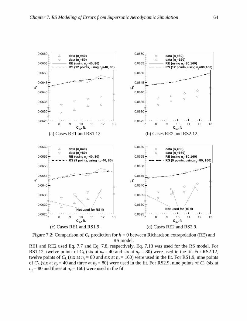
Chapter 7. RS Modeling of Errors from Supersonic Aerodynamic Simulation 64
Ctip, ft.
CL
7 8 9 10 11 12 130.0625
0.0630
0.0635
0.0640
0.0645
0.0650
0.0655
0.0660data (ny=40)data (ny=80)RE (using ny=40, 80)RS (12 points, using ny=40, 80)
(a) Cases RE1 and RS1.12.
Ctip, ft.C
L
7 8 9 10 11 12 130.0625
0.0630
0.0635
0.0640
0.0645
0.0650
0.0655
0.0660data (ny=80)data (ny=160)RE (using ny=80,160)RS (12 points, using ny=80,160)
(b) Cases RE2 and RS2.12.
Ctip, ft.
CL
7 8 9 10 11 12 130.0625
0.0630
0.0635
0.0640
0.0645
0.0650
0.0655
0.0660data (ny=40)data (ny=80)RE (using ny=40, 80)RS (9 points, using ny=40, 80)
Not used for RS fit
(c) Cases RE1 and RS1.9.
Ctip, ft.
CL
7 8 9 10 11 12 130.0625
0.0630
0.0635
0.0640
0.0645
0.0650
0.0655
0.0660data (ny=80)data (ny=160)RE (using ny=80,160)RS (9 points, using ny=80, 160)
Not used for RS fit
(d) Cases RE2 and RS2.9.
Figure 7.2: Comparison of CL prediction for h = 0 between Richardson extrapolation (RE) and RS model.
RE1 and RE2 used Eq. 7.7 and Eq. 7.8, respectively. Eq. 7.13 was used for the RS model. For RS1.12, twelve points of CL (six at ny = 40 and six at ny = 80) were used in the fit. For RS2.12, twelve points of CL (six at ny = 80 and six at ny = 160) were used in the fit. For RS1.9, nine points of CL (six at ny = 40 and three at ny = 80) were used in the fit. For RS2.9, nine points of CL (six at ny = 80 and three at ny = 160) were used in the fit.
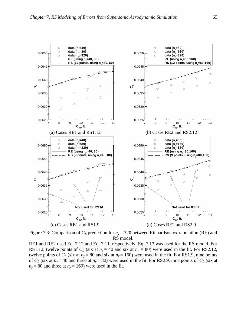
Chapter 7. RS Modeling of Errors from Supersonic Aerodynamic Simulation 65
Ctip, ft.
CL
7 8 9 10 11 12 130.0625
0.0630
0.0635
0.0640
0.0645
0.0650
data (ny=40)data (ny=80)data (ny=320)RE (using ny=40, 80)RS (12 points, using ny=40, 80)
(a) Cases RE1 and RS1.12
Ctip, ft.C
L
7 8 9 10 11 12 130.0625
0.0630
0.0635
0.0640
0.0645
0.0650
data (ny=80)data (ny=160)data (ny=320)RE (using ny=80,160)RS (12 points, using ny=80,160)
(b) Cases RE2 and RS2.12
Ctip, ft.
CL
7 8 9 10 11 12 130.0625
0.0630
0.0635
0.0640
0.0645
0.0650
data (ny=40)data (ny=80)data (ny=320)RE (using ny=40, 80)RS (9 points, using ny=40, 80)
Not used for RS fit
(c) Cases RE1 and RS1.9
Ctip, ft.
CL
7 8 9 10 11 12 130.0625
0.0630
0.0635
0.0640
0.0645
0.0650
data (ny=80)data (ny=160)data (ny=320)RE (using ny=80,160)RS (9 points, using ny=80,160)
Not used for RS fit
(d) Cases RE2 and RS2.9
Figure 7.3: Comparison of CL prediction for ny = 320 between Richardson extrapolation (RE) and RS model.
RE1 and RE2 used Eq. 7.12 and Eq. 7.11, respectively. Eq. 7.13 was used for the RS model. For RS1.12, twelve points of CL (six at ny = 40 and six at ny = 80) were used in the fit. For RS2.12, twelve points of CL (six at ny = 80 and six at ny = 160) were used in the fit. For RS1.9, nine points of CL (six at ny = 40 and three at ny = 80) were used in the fit. For RS2.9, nine points of CL (six at ny = 80 and three at ny = 160) were used in the fit.
Chapter 7. RS Modeling of Errors from Supersonic Aerodynamic Simulation 66
Ctip, ft.
CL
7 8 9 10 11 12 130.0625
0.0630
0.0635
0.0640
0.0645
0.0650
data (ny=40)data (ny=80)data (ny=320)RS on RE (using ny=40, 80)RS (12 points, using ny=40, 80)
(a) Cases RSRE1 and RS1.12
Ctip, ft.C
L7 8 9 10 11 12 13
0.0625
0.0630
0.0635
0.0640
0.0645
0.0650
data (ny=80)data (ny=160)data (ny=320)RS on RE (using ny=80,160)RS (12 points, using ny=80,160)
(b) Cases RSRE2 and RS2.12
Ctip, ft.
CL
7 8 9 10 11 12 130.0625
0.0630
0.0635
0.0640
0.0645
0.0650
data (ny=40)data (ny=80)data (ny=320)RS on RE (using ny=40, 80)RS (9 points, using ny=40, 80)
Not used for RS fit
(c) Cases RSRE1 and RS1.9
Ctip, ft.
CL
7 8 9 10 11 12 130.0625
0.0630
0.0635
0.0640
0.0645
0.0650
data (ny=80)data (ny=160)data (ny=320)RS on RE (using ny=80,160)RS (9 points, using ny=80,160)
Not used for RS fit
(d) Cases RSRE2 and RS2.9
Figure 7.4: Comparison of CL prediction for ny = 320 between RS fit to the Richardson extrapolation results (RSRE) and RS model.
RSRE1 and RSRE2 fit Eq. 7.15 to the results of RE1 (Eq. 7.12) and RE2 (Eq. 7.11), respectively. Eq. 7.13 was used for the RS model. For RS1.12, twelve points of CL (six at ny = 40 and six at ny = 80) were used in the fit. For RS2.12, twelve points of CL (six at ny = 80 and six at ny = 160) were used in the fit. For RS1.9, nine points of CL (six at ny = 40 and three at ny = 80) were used in the fit. For RS2.9, nine points of CL (six at ny = 80 and three at ny = 160) were used in the fit.

67
Chapter 8 Test Problem Study of Errors from
Optimization Failures
Most engineering optimization problems require iterative algorithms that may be difficult
to converge to high precision due to computational cost. A sub-optimization problem is often
solved within a system level optimization. For example, structural optimization was used to
calculate optimal wing structural weight within the configuration optimization of the HSCT.
Poor results from the nested sub-optimization may cause design uncertainties of the system. In
this chapter, a simple test problem is used as an example of optimization errors. The statistical
methods introduced in Chapters 5 and 6 will be used to estimate and reduce the optimization
errors.
8.1 Errors of Various Optimization Methods on the Rosenbrock
Function
Before addressing the HSCT problem, it is worthwhile to illustrate the convergence
difficulties experienced by numerical optimization for a simple problem. Here we demonstrate
the failure of some optimization algorithms for a simple unconstrained minimization problem,
the generalized Rosenbrock function [58] in five dimensions:
[ ] ).5( , )1()(100)(1
1
2221 =−+−= ∑
−
=+ nxxxf
n
kkkkx (8.1)
The unconstrained minimization problem has a unique optimum x* = (1, 1, 1, 1, 1) at
which f* = f(x*) = 0. We performed 500 runs from different initial points, which were randomly
generated in the range of [0, 2]5, to check for any optimization failures. As a criterion of failure,
we used f* > 0.0001 such that only runs with meaningful error, not due to finite convergence
criteria of the optimization algorithm, are declared as failures. For the purpose of this
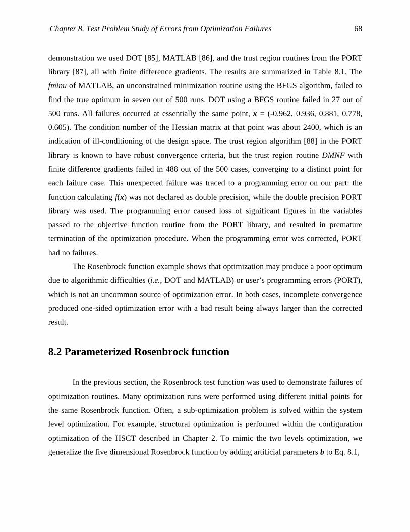
Chapter 8. Test Problem Study of Errors from Optimization Failures 68
demonstration we used DOT [85], MATLAB [86], and the trust region routines from the PORT
library [87], all with finite difference gradients. The results are summarized in Table 8.1. The
fminu of MATLAB, an unconstrained minimization routine using the BFGS algorithm, failed to
find the true optimum in seven out of 500 runs. DOT using a BFGS routine failed in 27 out of
500 runs. All failures occurred at essentially the same point, x = (-0.962, 0.936, 0.881, 0.778,
0.605). The condition number of the Hessian matrix at that point was about 2400, which is an
indication of ill-conditioning of the design space. The trust region algorithm [88] in the PORT
library is known to have robust convergence criteria, but the trust region routine DMNF with
finite difference gradients failed in 488 out of the 500 cases, converging to a distinct point for
each failure case. This unexpected failure was traced to a programming error on our part: the
function calculating f(x) was not declared as double precision, while the double precision PORT
library was used. The programming error caused loss of significant figures in the variables
passed to the objective function routine from the PORT library, and resulted in premature
termination of the optimization procedure. When the programming error was corrected, PORT
had no failures.
The Rosenbrock function example shows that optimization may produce a poor optimum
due to algorithmic difficulties (i.e., DOT and MATLAB) or user’s programming errors (PORT),
which is not an uncommon source of optimization error. In both cases, incomplete convergence
produced one-sided optimization error with a bad result being always larger than the corrected
result.
8.2 Parameterized Rosenbrock function
In the previous section, the Rosenbrock test function was used to demonstrate failures of
optimization routines. Many optimization runs were performed using different initial points for
the same Rosenbrock function. Often, a sub-optimization problem is solved within the system
level optimization. For example, structural optimization is performed within the configuration
optimization of the HSCT described in Chapter 2. To mimic the two levels optimization, we
generalize the five dimensional Rosenbrock function by adding artificial parameters b to Eq. 8.1,

Chapter 8. Test Problem Study of Errors from Optimization Failures 69
[ ] ).,,,( where,)1()(100);(4
14321
2221∑
=+ =−+−=
kkkkk bbbbxxbxf bbx (8.2)
If we define
);(min)( bxbx
ffo ≡ , (8.3)
there are two levels of optimization; b* is sought to minimize fo(b) in the upper level, and x* is
sought to minimize f for a given b to find fo(b) in the lower level. b corresponds to the
configuration design variables of the HSCT in the system level and x corresponds to the design
variables of the structural optimization, the sub-optimization. Assume that we want to find b that
minimizes fo(b), and we may want to build a response surface approximation of fo(b) with respect
to b as we do for the optimal wing structural weight of the HSCT.
We elected to change only b1, b2, and b3, while keeping b4 = 1, to make fo(b) have a
unique minimum of zero at (b1, b2, b3 ) = (1, 1, 1). The ranges of bk’s are chosen to be between
0.9 and 1.1. For a given set of bk’s, the parameterized Rosenbrock function is minimized from an
initial design point x = (1.1, 0.9. 1.1, 0.9. 1.1). Figure 8.1 is a design line plot of fo showing the
noisy response of fo(b1, b2, b3) when PORT with the programming error was used. It is a one-
dimensional cut of the fo response on eleven data points linearly interpolated between b = (0.9,
0.9, 0.9) and b = (1.1, 1.1, 1.1). The true response corresponds to results of PORT without the
programming error. We can see that PORT with the programming error gave satisfactory results
for only two out of the eleven runs. Define the optimization error
t
oe
o ffe −= , (8.4)
where foe is the result of the erroneous PORT and fo
t is the result of the correct PORT. It is
apparent that poor optimizations result in heavier designs and the optimization error is one-sided.

Chapter 8. Test Problem Study of Errors from Optimization Failures 70
8.3 Estimation of the Optimization Error
We found that the user’s programming mistake resulted in poor convergence in PORT
optimization runs. The fact that optimization errors are noisy and one-sided leads us to use
probabilistic modeling with appropriate candidate distributions. Once we find a probabilistic
model of the error, it can be incorporated into a robust design study. Also, we will demonstrate
that the probabilistic model is useful to estimate the average error of the optimization runs.
To measure the error of PORT on the parameterized Rosenbrock function, we need
sample optimization runs. We used 125 (= 5×5×5) data points from a full factorial experimental
design of five levels in b. PORT with the programming error was performed to calculate fo for
each of the 125 variants of the parameterized Rosenbrock function. Two sets of 125 data points
were generated by using two different initial x’s: Case 1 using x0 = (1.1, 0.9, 1.1, 0.9, 1.1) and
Case 2 using x0 = (0.9, 1.1, 0.9, 1.1, 0.9). Case 2 will be used to demonstrate the indirect
approach of distribution fit in Section 8.3.3. Also, PORT without the programming error
(denoted Case 0) was performed to calculate the error of Case 1 and Case 2 according to Eq. 8.4.
The errors were large compared to the true fo, whose average is 0.00399; the average error of
Case 1 and Case 2 was 0.00658 (164.9%) and 0.00505 (126.6%), respectively. The low fidelity
optimizations of Cases 1 and 2 cost as much computationally as the high-fidelity optimization of
Case 0 (Table 8.2). The average number of function evaluations of Case 0 was 199, which is
comparable to 209 of Case 1 or 187 of Case 2. Some of the function evaluations might have been
wasted for Case 1 and Case 2, because the programming error of the low fidelity cases results in
less accurate gradients.
8.3.1 Homogeneity of the Error Distribution
We selected the Weibull distribution as a model for the optimization error of PORT. It is
defined for a nonnegative random variable and has great flexibility (see Figure 5.2). The
parameters of the model function are found by the maximum likelihood estimate (MLE). A basic
assumption of the MLE fit introduced in Section 5.3 is that the data is independently and

Chapter 8. Test Problem Study of Errors from Optimization Failures 71
identically distributed. For the optimization data of the parameterized Rosenbrock function, the
dependence of the data may not be a problem, since the sampling was done by an experimental
design without replicates. To check whether the error distribution is the same at different points,
the optimization error, e, is plotted against the true fo in Figure 8.2(a) for Case 1 and Figure
8.2(b) for Case 2. Although there seems to be a few outliers, homogeneity of the error
distribution appears to be a reasonable assumption. The correlation between e and the true fo was
low: 0.1635 for Case 1 and –0.0264 for Case 2.
8.3.2 Results of Direct Fit of PORT Optimization Error
A Weibull model was fit to the distribution of optimization errors of Case 1 and Case 2
using the weibfit routine of MATLAB [89], and the results are summarized in Table 8.3. The two
parameters of the Weibull model, a shape parameter α, and a scale parameter β, were estimated
via MLE. From the estimated parameters, α and β , estimates of the mean ( fitµ ) and standard
deviation ( fitσ ) of the error can be calculated using the formulas in Table 5.1. According to the
p-values of the χ2 goodness-of-fit test, the fit to Case 1 was marginally rejected at the 0.05
significance level, while the fit to Case 2 was reasonable.
Recalling that the standard deviation is the same as the mean for the exponential
distribution (when α = 1 in Weibull), fitσ greater than fitµ indicates that the optimization errors
have greater scatter than the exponential model. The overall characteristics of the error can be
identified using fitµ and fitσ from the MLE fit. On the other hand, the mean and standard
deviation can be estimated directly from e by
1
)(ˆ,ˆ 1
2
−
−==
∑=
n
eee
n
ii
datadata σµ . (8.5)
In Table 8.3, fitµ and fitσ were compared with dataµ and dataσ . The agreement is good except for
the standard deviation of Case 1, with 35.6% discrepancy.
The histograms in Figure 8.3 compare the shape of the error distribution to the Weibull
fit. The optimization error is nonnegative, and the probability for large error decreases rapidly to

Chapter 8. Test Problem Study of Errors from Optimization Failures 72
zero. Although the fit to Case 1 was marginally rejected by the χ2 test, the frequencies predicted
by the direct fit show a reasonable match with the data in Figure 8.3(a). The fit to Case 2 in
Figure 8.3(b) describes the data pretty well.
It should be noted that the above discussions about the results of χ2 tests and the
corresponding p-values are not rigorous probability statements, because it is possible that the
sample size n is not large enough for the asymptotic χ2 approximation to be accurate.
Nevertheless, whether the true distribution is Weibull or not, the Weibull model does represent
the data well and therefore may find usefulness in error modeling.
8.3.3 Results of Indirect Fit of PORT Optimization Error
The direct approach in Section 8.3.2 requires accurate optimization results to estimate the
error. Sometimes, however, we do not have high-fidelity runs because we simply do not know
how to improve the accuracy of the simulation. Assume that we do not know of the
programming error that resulted in erroneous results from PORT. Then, we can use the pair of
Cases 1 and 2 to estimate the error via the indirect fit (Section 5.6). Note that Case 2 uses a
different initial x from Case 1. To reduce possible dependence of the errors between Case 1 and
Case 2, the initial x of Case 2 was set such that each xi was opposite to that of Case 1. The
correlation between e1 (error of Case 1) and e2 (error of Case 2) was small, -0.0371.
The results of the difference fit using the Weibull model are shown in Table 8.4. Note
that the distribution parameters α and β of Case 1 and Case 2 are simultaneously estimated.
Because there is no closed form of the probability density of the difference for the Weibull
model, Eq. 5.12 was numerically integrated using Gaussian quadrature (Ref. [57], pp. 222-228).
See Appendix C for the details of the integration method. According to the χ2 test, the indirect fit
was reasonable with a p-value of 0.4357.
From results of the indirect fit, we can estimate the mean and standard deviation of the
optimization error of the two cases involved (Table 8.5), which can be compared to the estimates
from data using Eq. 8.5. The estimates for Case 1 were reasonable with 2.7% discrepancy for the
mean (µ) and 6.1% discrepancy of the standard deviation (σ). The estimates for Case 2 were in
closer agreement with a 2.0% discrepancy for µ and a 0.9% discrepancy for σ. The results

Chapter 8. Test Problem Study of Errors from Optimization Failures 73
demonstrate the usefulness of the probabilistic model for the optimization error. By
incorporating the probability model into the indirect fit, we were able to estimate the error
without obtaining accurate optimization results.
Compared to the results of the direct fit (Table 8.3), the indirect fit gave more accurate
estimates of µ and σ for this particular example. For example, the direct fit had discrepancies of
5.2% and 35.6% for µ and σ, respectively in Case 1, while the discrepancies of the indirect fit
were 2.7% and 6.1%, respectively. However, the result may not be generalized to other
problems. In fact, we expect the direct fit to be as good as the indirect fit if the error data is
accurately measured, because the sample size for the indirect approach is the same as that of the
direct fit in MLE, while the number of parameters estimated is doubled.
8.4 Detection and Repair of Erroneous Optimization Runs
The robust regression techniques are demonstrated using SAS [90] statistical software to
identify erroneous optimizations of PORT with the programming error. To construct a quadratic
response surface approximation of fo(b1, b2, b3), 27 variants of the Rosenbrock function are
generated by using a three level full factorial design in bk, (k = 1, 2, 3). Two different weighting
functions from Table 6.1 are compared: the biweight function (denoted IRLS) and the
nonsymmetric weighting function (denoted NIRLS). The identified outliers having IRLS/NIRLS
weighting less that 0.01 are repaired using the correct PORT optimization.
Table 8.6 summarizes the results of outlier repair. Before outlier repair, the root mean
square error (RMSE) of the quadratic response surface was 54.3% and the R2 value was only
0.68. Because many data points suffered from poor optimization, an aggressive outlier search
was performed using a lower value of the tuning constant B = 1.0. We defined big outliers as
those showing 10% or greater error. 20 out of 27 data points satisfied this criterion. IRLS
declared 9 points as outliers but only 7 of them were big outliers, while NIRLS detected 8
outliers and all of them were big outliers. Note that the mean repair on the outliers by NIRLS is
0.0213 while the mean repair on the outliers by IRLS is only 0.0124. By utilizing the one-
sidedness of the error, NIRLS is more successful than the symmetric weighting function of
IRLS. The data points not declared as outliers will be called inliers. The ratio of average repairs

Chapter 8. Test Problem Study of Errors from Optimization Failures 74
between outliers and inliers can be considered as a measure of success of outlier detection. For
NIRLS the ratio was 7.02 compared to 1.91 of IRLS. The response surface fit is improved via
IRLS repair, and there is still substantial improvement by NIRLS repair over IRLS repair; the
RMSE is 45.5% for IRLS repair and 29.7% for NIRLS repair. When all 27 points were repaired,
the RMSE was only 4.3% and the R2 was 0.9970.
8.5 Effects of Outlier Repair on the Quality of the Optimum of RS
Approximation
The response surface approximations are compared in Figure 8.5 along the same design
line used for Figure 8.1. Before outlier repair the response surface approximation over-predicts
the true response because of the data points of positive error. With IRLS repair, the response
surface prediction is improved but the trend of the response is not accurate. The response surface
fit with NIRLS repair follows the true response closely. The response surface models are to be
used to find the minimum of fo(b1, b2, b3). It is clear from the figure that the response surface fit
with NIRLS repair will find a more accurate optimum fo* than the response surface fit with IRLS
repair. Table 8.7 summarizes the results of minimization of fo according to the response surface
models used. When using the response surface fit without repair, the optimum of fo is located at
the boundary of the design space of b, which have ranges between 0.9 and 1.1. Considering that
the true optimum is located at the center of the design box, the original response surface
approximation completely failed to capture the trend of the true response. It is seen that fo* gets
closer to the true optimum as more outliers are repaired. Comparing the accuracy at optima fo*,
the response surface model with IRLS repair under-predicts the response by 0.00257 = 0.00082 -
(-0.00175) while the error of NIRLS is only 0.00046 = 0.00028 - (-0.00018).

Chapter 8. Test Problem Study of Errors from Optimization Failures 75
Table 8.1: Failure of various optimization programs for the five dimensional Rosenbrock function.
Software MATLAB (fminu) DOT PORT
(DMNF)
Algorithm BFGS BFGS Trust region
Options - - With
programming error
Programming error corrected
Number of failures out of 500 runs 7 27 488 0
Table 8.2: Summary of PORT runs for 125 variants of the parameterized Rosenbrock function. Cases Case 0 Case 1 Case 2
Algorithm Trust region Trust region Trust region
Description Programming error corrected
With programming error,
x0 = (1.1, 0.9, 1.1, 0.9, 1.1)
With programming error,
x0 = (0.9, 1.1, 0.9, 1.1, 0.9)
Average error of fo
(% compared to the average of
true fo)
- 0.00658 (164.9%)
0.00505 (126.6%)
Average number of function evaluation
199 209 187

Chapter 8. Test Problem Study of Errors from Optimization Failures 76
Table 8.3: Fits of the Weibull model to the error from PORT optimization of the parameterized Rosenbrock function.
Case 1 and Case 2 use different initial designs. fitµ and fitσ are estimates from the fit of the
Weibull distribution, while dataµ and dataσ are estimates from the data using Eq. 8.5. The estimates of mean, µ, from the fit are in good agreement for both Cases 1 and 2. The estimates of the standard deviation, σ, is also reasonable for Case 2. The p-value of the χ2test indicates the fit is particularly good for Case 2.
Case 1 x0 = (1.1, 0.9, 1.1, 0.9, 1.1)
Case 2 x0 = (0.9, 1.1, 0.9, 1.1, 0.9)
dataµ 0.00658 0.00505
fitµ
(discrepancy w.r.t dataµ ) 0.00692 (5.2 %)
0.00496 (-1.8 %)
dataσ 0.00752 0.0110
fitσ
(discrepancy w.r.t dataσ ) 0.0102 (35.6%)
0.0102 (-7.3 %)
α (shape parameter) 0.6941 0.5297 β (scale parameter) 0.005421 0.002744
χ2 statistic 14.76 4.68 p-value 0.0392 0.6989

Chapter 8. Test Problem Study of Errors from Optimization Failures 77
Table 8.4: Results of the indirect fit for the optimization error of PORT. The p-value of the χ2test indicates that the fit is acceptable.
Case 1 α
β
0.8507
0.006214
Case 2 α
β
0.5134
0.002698
χ2 statistic 4.84
p-value 0.4357

Chapter 8. Test Problem Study of Errors from Optimization Failures 78
Table 8.5: Comparison of the estimates of mean ( fitµ ) and the estimates of standard deviation
( fitσ ) from indirect fit with dataµ and dataσ (see Eq. 8.5). The indirect fit gave good estimates of mean error for both Case 1 and Case 2.
Cases Case 1 Case 2
dataµ 0.00658 0.00505
fitµ from indirect fit
(discrepancy w.r.t dataµ )
0.00676
(2.7%)
0.00515
(2.0%)
dataσ 0.00752 0.0110
fitσ from indirect fit
(discrepancy w.r.t dataσ )
0.00798
(6.1%)
0.0111
(0.9 %)
Table 8.6: Results of outlier repair for the parameterized five dimensional Rosenbrock function.
B
Number of
outliers
a/b/c*
Mean of repair
on outliers†
Mean of repair
on inliers‡
Ratio of mean
repair on OL to
IL
RMSE
(% to the
mean fo)
mean fo R2
Before
repair NA NA NA NA NA
0.00748
(54.3%) 0.0138 0.6800
IRLS
repair 1.0 9/7/20 0.0124 0.0065 1.91
0.00439
(45.5%) 0.0096 0.8342
NIRLS
repair 1.0 8/8/20 0.0213 0.0030 7.02
0.00222
(29.7%) 0.0075 0.8658
Full
repair§ NA NA NA NA NA
0.00023
(4.3%) 0.0053 0.9970
*: a ~ Number of detected outliers b ~ Number of big outliers detected (estimated error is greater than 10%) c ~ Total number of big outliers out of the 27 data points (estimated error is greater than 10%) †: (Sum of fo repair on outliers)/a ‡: (Sum of fo repair on data points other than outliers)/(Total number of points - a) §: All 27 points repaired

Chapter 8. Test Problem Study of Errors from Optimization Failures 79
Table 8.7: Results of optimization of fo(b1, b2, b3) from the parameterized Rosenbrock function using RS approximations before and after outlier repair.
Without
repair
(Optimum O)
IRLS repair
(Optimum I)
NIRLS repair
(Optimum N)
Full repair
(Optimum F) Exact
b1* 0.9583 0.9922 1.0014 1.0057 1.0
b2* 1.1000 1.0591 0.9877 1.0072 1.0
b3* 0.9000 0.9965 1.0378 1.0060 1.0
fo(b1* , b2
* , b3*)
predicted by RS 0.00066 -0.00175 -0.00018 -0.00007 -
fo(b1* , b2
* , b3*)
True 0.00303 0.00082 0.00028 0.00005 0.0

Chapter 8. Test Problem Study of Errors from Optimization Failures 80
design
f o
1 2 3 4 5 6 7 8 9 10 11-0.01
0.00
0.01
0.02
0.03
0.04
DataTrue
Figure 8.1: Design line plot of the optimal values (fo) for the parameterized Rosenbrock function. Design 1 corresponds to bk’s at their lower limits and design 11 corresponds to bk’s at their upper limits. Noisy data are the results of PORT with a programming error, and the solid line is the true optima.

Chapter 8. Test Problem Study of Errors from Optimization Failures 81
+
+
+
++
++
+
+ +
++
+
+
+
+++
+
+
+
++ +
+
+
+
+
+
+
+++
+
+
+
+
+
+
+
+++
++
+++
+
+
+
+
++
+
+
+++
+
+
+
++
+
+++ +
+
+++
+
+
+
++
+
+ ++
+
+ ++
+
+
+ +++
+
+ ++
+ +
+
+
+
++
+
+ +
+
+
+
+
+
+
+
++
+
+
+
++
+
+ +
+
+
fo, true
Err
orof
fo
0.000 0.005 0.010 0.015 0.0200.000
0.005
0.010
0.015
0.020
0.025
0.030
0.035
0.040
(a) Case 1 (correlation = 0.1635)
++
+
++ ++++ + ++++ + +
+
+ + ++
+
+ + + +++++
+
+++ + ++++ ++
+
+
+
++
+
+ + ++++++ +
+++ + ++
+
+
++++ +
+
+
+
++
+ ++++ + ++
++ + ++
+ + ++
+
+ ++
+
+
+
+ ++++++ +
+++
++
+
+ + +
+
+
+ +
+
++ ++
+
fo, true
Err
orof
fo
0.000 0.005 0.010 0.015 0.0200.00
0.01
0.02
0.03
0.04
0.05
0.06
0.07
0.08
0.09
0.10
(b) Case 2 (correlation = -0.0264)
Figure 8.2: Plots of optimization error versus estimated true fo.
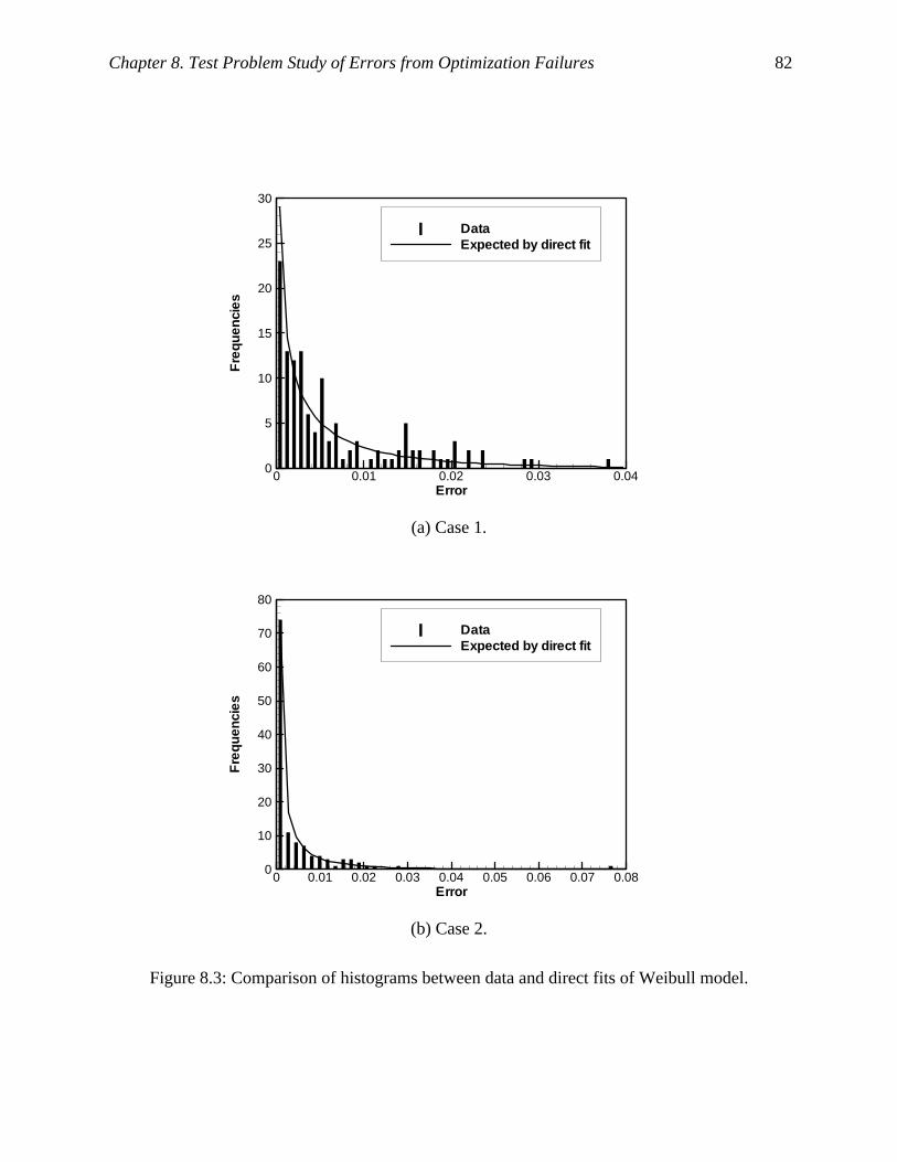
Chapter 8. Test Problem Study of Errors from Optimization Failures 82
Error
Fre
quen
cies
0 0.01 0.02 0.03 0.040
5
10
15
20
25
30
DataExpected by direct fit
(a) Case 1.
Error
Fre
quen
cies
0 0.01 0.02 0.03 0.04 0.05 0.06 0.07 0.080
10
20
30
40
50
60
70
80
DataExpected by direct fit
(b) Case 2.
Figure 8.3: Comparison of histograms between data and direct fits of Weibull model.
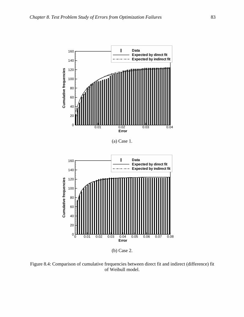
Chapter 8. Test Problem Study of Errors from Optimization Failures 83
Error
Cum
ulat
ive
freq
uenc
ies
0.01 0.02 0.03 0.040
20
40
60
80
100
120
140
160 DataExpected by direct fitExpected by indirect fit
(a) Case 1.
Error
Cum
ulat
ive
freq
uenc
ies
0 0.01 0.02 0.03 0.04 0.05 0.06 0.07 0.080
20
40
60
80
100
120
140
160 DataExpected by direct fitExpected by indirect fit
(b) Case 2.
Figure 8.4: Comparison of cumulative frequencies between direct fit and indirect (difference) fit of Weibull model.
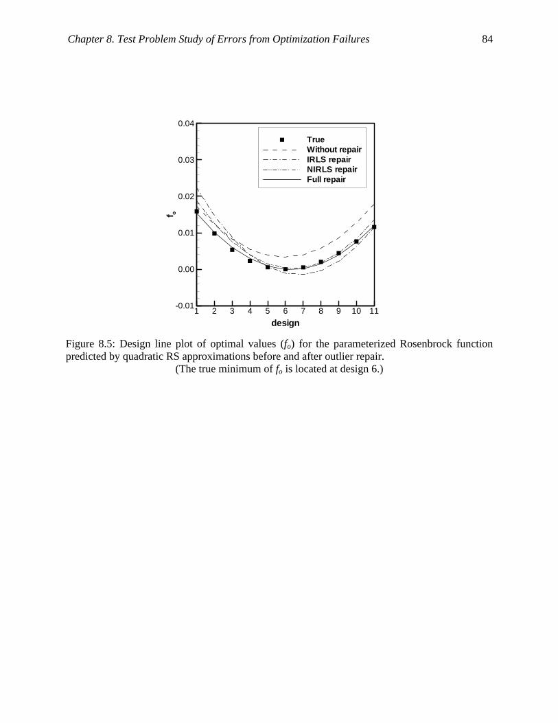
Chapter 8. Test Problem Study of Errors from Optimization Failures 84
design
f o
1 2 3 4 5 6 7 8 9 10 11-0.01
0.00
0.01
0.02
0.03
0.04
TrueWithout repairIRLS repairNIRLS repairFull repair
Figure 8.5: Design line plot of optimal values (fo) for the parameterized Rosenbrock function predicted by quadratic RS approximations before and after outlier repair.
(The true minimum of fo is located at design 6.)

85
Chapter 9 Estimation of Error from Structural
Optimization
The error from structural optimization of the HSCT resulted in unreliable estimates of the
wing structural weight. The source of the error was investigated by using various convergence
parameters. Convergence difficulties in optimization procedures would produce one-sided noise
error. A probabilistic approach is used to model the noise error from structural optimization. The
Weibull model successfully used for the Rosenbrock test problem will be applied.
9.1 Effects of Convergence Control Parameters on the Optimization
Error
We found that the error of structural optimization depends on the convergence criteria,
which are called control parameters in GENESIS. The noise in the optimum structural wing
weight (Ws) of an HSCT was greatly reduced by adjusting the GENESIS settings. Control
parameters in GENESIS can be categorized into move limit parameters, convergence criteria,
and inner optimization control parameters. Since we are dealing with a convergence problem of
optimization, it will be helpful to understand the program structure of GENESIS. There are two
loops in GENESIS (Figure 9.1). In the outer loop, an approximation for the optimization
problem is generated and this approximate problem is passed to the inner loop of a gradient
based optimization. We used the modified method of feasible direction (MMFD) for the inner
loop optimization. After convergence of the approximate problem, a new approximation is
constructed at the optimum of the approximate problem. The approximation and optimization is
continued until no further change of design variables, called soft convergence, or no further
change of the objective function, called hard convergence, occurs. The optimization parameters
affect the performance of optimization, error in the optimization results, and the computational
cost.

Chapter 9. Estimation of Error from Structural Optimization 86
To study the error in the optimal structural weight calculation of the HSCT, we used a
mixed experimental design [45] designed to permit fitting quadratic or cubic polynomial models
using the five HSCT configuration design variables. The experimental design has 126 points that
consist of a face centered central composite design (FCCC) at levels of ±1 (43 points), another
FCCC at levels of ±0.75 (42 points), a D-optimal design from a 6 level design (27 points), and an
orthogonal array design [91] (14 points).
GENESIS structural optimizations using six different sets of parameters were performed
on each of the 126 points. Table 9.1 lists the description of the parameters and the actual values
used in this study. Case A2 employs the default parameters provided by GENESIS. Case A3 and
Case A5 are the same as Case A2 except that the parameter ITRMOP was increased to 3 and 5,
respectively. ITRMOP controls the convergence of the inner optimization. For the approximate
optimization to converge, the inner loop convergence criterion for change in the objective
function must be satisfied ITRMOP consecutive times. The default value of ITRMOP is 2, and
by increasing it, the inner iteration is forced to iterate further. In turn, this may force the outer
loop to continue, because the so called soft convergence criteria −the change of design variables−
are not met, which may have been satisfied if ITRMOP had been 2. This may result in significant
improvement in the final design.
After extensive experimentation with the optimization parameters and help from the
developers of GENESIS, we found that ITRMOP was the most important for improving the
accuracy of the optimization for our problem. Case B2 employs tighter move limits and
convergence criteria than Case A2. It reflects our first attempt to improve the optimization
results. Case B3 and Case B5 are the same as Case B2 except that ITRMOP is 3 and 5,
respectively. The values of all the control parameters for the six cases are given in Table 9.1. The
data of Ws of the six convergence settings on the 126 data points are listed in Appendix D.
In order to visualize the behavior of the errors, Figures 9.2(a) and (b) show the Ws
response for 21 HSCT designs generated by linear interpolation between two extreme points in
the five variable HSCT problem. It is the same design line used for Figure 3.4 and design 1
corresponds to (1, -1, 1, -1, 1) and design 21 corresponds to (-1, 1, -1, 1, -1) in a coded form of
the HSCT configuration variables. It is clear from the figures that Case A2 and Case B2
produced many runs with large errors, which were mostly positive. GENESIS seeks optimal
design within feasible region because we use MMFD algorithm. There was no run for which

Chapter 9. Estimation of Error from Structural Optimization 87
GENESIS failed to find a feasible design, and all of the erroneous optima were feasible.
Therefore, the one-sided error in Ws calculated from GENESIS is attributed to convergence
problem. By increasing ITRMOP, the noise in Ws was substantially reduced and the gain with
ITRMOP = 5 over ITRMOP = 3 was small. To calculate the error for each case, we need to
know the true Ws, which, strictly speaking, cannot be known due to the iterative procedure
inherent in the optimization. Here we estimate the true Ws by taking the best of the six GENESIS
runs we already did using different parameters.
Table 9.2 shows the performance of each set of GENESIS parameters for all 126 design
points. The optimization error was calculated by comparing Ws to the best of the six Ws’s
available. Table 9.2 shows how many times each case produced the lowest weight, the best
among the six Ws’s for 126 points. Case A2 and Case B2 never found the best results. With
ITRMOP = 5, Case A5 and Case B5 achieved the best Ws 58 and 52 times respectively, almost
half of the data each, and together nearly 90 % of the data. Sometimes Case A3 and Case B3
came up with the best results, for 12 and 4 times, respectively.
For the default GENESIS parameter (Case A2), the mean error was 4.86 %. It is seen that
tightening the convergence criteria for ITRMOP = 2 (Case B2) actually had a detrimental effect
since the mean error increased to 5.63 %. By using ITRMOP = 3 (Case A3 and Case B3), the
mean errors were reduced to 0.546 % and 0.762 % respectively, about a tenth of the levels of the
low-fidelity errors. With Case A5 and Case B5, the mean error was very small, less than 0.2%. In
terms of computational cost, the high-fidelity optimization using ITRMOP = 5 required more
than twice the CPU time of the low-fidelity optimization, ITRMOP = 2.
In fact, the estimate of the true optimum by taking the best of six runs turned out to be
very accurate, mostly thanks to the high-fidelity of Case A5 and Case B5. This was tested by
doing nine additional GENESIS runs on 30 randomly selected HSCT configurations using Case
B5 from different initial design variables. For these 30 configurations an average of 0.011%
improvement was obtained. Therefore, we will denote the best of six Ws’s as ‘the estimate of true
Ws’, and accordingly the error of Ws with respect to this value will be denoted as ‘estimated
error’, et, of optimization. Our concern about uncertainly will be mainly for the low (ITRMOP =
2) and mid-fidelity (ITRMOP = 3) cases. For the high-fidelity cases (ITRMOP = 5), the error
appears to be negligible.

Chapter 9. Estimation of Error from Structural Optimization 88
9.2 Estimation of Statistical Distribution
9.2.1 Homogeneity of Error
Our approach is to fit a model function to optimization error of various optimization
convergence setups. A basic assumption behind the MLE fit is that the data is independently and
identically distributed. For the optimization data at hand, there should be no problem concerning
the independence of data, because the sampling was done by an experimental design without
replicates. To check whether the error distribution is identical at different points, the estimated
errors, et, were plotted against the estimated true Ws in Figure 9.3 for the absolute error (lb.) and
in Figure 9.4 for the relative error (%). For example, with the absolute error of Case A2 in Figure
9.3(a), the mean and variance of error appears to increase as Ws increases. A relatively high
correlation coefficient of 0.5685 indicates the trend. Scaling the error by Ws may help to stabilize
the increasing mean and variance along Ws. For the relative error of Case A2 in Figure 9.4(a), the
distribution became more even, and the correlation coefficient was reduced to 0.3210. One may
observe similar effects of relative error over absolute error for other cases. The figures lead us to
expect that if the structural optimization process ends with premature convergence, the absolute
error would tend to be larger for heavy designs.
However, considering that highly influential points, such as the two outliers seen in
Figure 9.3(b), tend to exaggerate the correlation coefficients, the assumption of homogeneous
distribution may not be a bad assumption even for the absolute error. If the variation of
distribution is important, the change of distribution may be modeled by the generalized linear
model (GLM) [92]. In GLM the mean of the distribution is related to the regressor variables via a
linear model, while the fit in our approach assumes the mean of the distribution is the same for
different data points, which is a special case of GLM. Nonetheless, with the four distributions in
Figure 9.3, the fit of a distribution should provide useful information about the overall behavior
of the error. So we fitted model distributions to both absolute and relative errors.

Chapter 9. Estimation of Error from Structural Optimization 89
9.2.2 Direct Fit of Estimated Error
In Chapter 8 the Weibull model was successfully fit to the optimization error of the
Rosenbrock function. Again, the Weibull model is selected to fit the estimated error et, from the
structural optimization of the HSCT. The results of the direct fit are summarized in Table 9.3 for
the absolute error, and in Table 9.4 for the relative error. A Weibull model fit routine, weibfit,
from the statistical toolbox of MATLAB was used. See Appendix E for an example of the
MATLAB code for the direct fit. For the absolute error, the p-values of the χ2 test indicate that
the fits are reasonable for Cases A2, B2, and B3 with 5% significance level. For Case A3, the fit
was marginally rejected. For Case A5 and Case B5, the high-fidelity cases with ITRMOP = 5,
the fits were not satisfactory at all. In fact, for those high-fidelity errors, almost half of the et’s
were zero, and the errors may be negligible. The Weibull fit of the relative error was not as good
as the fit for the absolute error. For instance, the p-value of the fit to the relative error of Case B2
was only 0.0327 compared to 0.8327 for the fit to the absolute error. This is unexpected since we
observed that the distribution appears to be more homogeneous with relative error than with
absolute error.
Recalling that the standard deviation is the same as the mean for the exponential
distribution (when α = 1 in Weibull), fitσ greater than
fitµ in Table 9.3 indicates that the errors
from the structural optimization have greater scatter than the exponential model. From the fits,
overall characteristics of the error can be estimated in terms of the mean (fitµ ), and standard
deviation (fitσ ) of the distribution. On the other hand, the mean and standard deviation can be
estimated from et without fit by
1
))((ˆ,ˆ 1
2
−
−==
∑=
n
eee
n
itit
datatdata σµ . (9.1)
In Table 9.3, fitµ and
fitσ were compared with dataµ and
dataσ , and the agreement is good for low-
fidelity errors and is reasonable for the mid-fidelity errors except for fitσ of Case B3.

Chapter 9. Estimation of Error from Structural Optimization 90
Table 9.3 and Table 9.4 are obtained from 126 data points. We expect that fewer points
are required for a reasonable fit to estimate the mean and standard deviation of the error
distribution. For a given sample size ranging from 10 to 150, we calculated fitµ and
fitσ for 50
sets of random numbers generated from a Weibull distribution with α = 0.7682 and β = 3915,
which is the fitted value for et of Case B2. The mean (µ) and standard deviation (σ) of the
distribution are 4572 lb. and 6023 lb., respectively. The mean and standard deviation of fitµ are
drawn in Figure 9.5(a) as dash-dot lines. Similarly the mean and standard deviation of fitσ are
shown in Figure 9.5(b). It appears that we need at least 50 points to get a good fit with
reasonable accuracy. Also, Figure 9.5(a) shows that the mean and scatter of dataµ are very close to
those of fitµ , but Figure 9.5(b) shows that
fitσ has a smaller scatter than dataσ in terms of the
standard deviation.
The probability plot is a graphical tool to show the goodness of fit of distribution. We
used the quantile-quantile plots, or so-called Q-Q plot (see Section 5.5). In the Q-Q plot, the
percentiles of the data are plotted against the expected percentiles from the fit. If the fit is good,
the scatter plot should appear as a straight line passing the origin with unit slope. Figure 9.6
shows the Q-Q plots for the Weibull fit for et of the low and mid-fidelity optimizations. They
show that the MLE resulted in a good fit for the majority of the data, while more or less ignoring
the large error data. Figure 9.6(c) indicates a particularly good fit, which is in agreement with the
results of the χ2 test. The histograms in Figure 9.7 compare the shape of the error distribution to
the Weibull fit. The optimization error here is by definition nonnegative and the probability for
large error decreases rapidly to zero. One can see that the fits match well with the data for the
low-fidelity errors, Case A2 and Case B2, and the fits are reasonable for the mid-fidelity error
cases, even for Case A3, although the fit was rejected by the χ2 test. This fact implies that the
Weibull fit may be useful for Case A3 as well if we are mainly interested in the behavior of large
error.
Again, it should be noted that the above discussions about the results of χ2 tests and the
corresponding p-values are not rigorous probability statements, since the sample size n may not
be large enough for the asymptotic χ2 approximation to be accurate. However, the Weibull
distribution was able to model the errors of two different optimization problems, the Rosenbrock

Chapter 9. Estimation of Error from Structural Optimization 91
function and the structural optimization of an HSCT. That may be an indication that there are
some common error processes in the optimization errors.
9.2.3 Results of Indirect Fit of the Optimization Error
In our data, Case A3 and Case B2 represent our efforts to reduce the error in Case A2 by
tightening the inner loop convergence criterion or outer loop criteria. If either optimization
results by Case A3 or Case B2 are available along with Case A2, we can estimate the error
distributions from the differences. Note that we use two sets of different convergence criteria,
while we used two cases of different initial designs for the Rosenbrock example. Similarly to
what was done for the Rosenbrock problem, the probability density of the difference, f(x) in Eq.
5.12, was numerically integrated using the Gaussian quadrature (see Appendix C for the details
of the integration). Table 9.5 contains the correlation of et between the low and mid-fidelity
optimizations, Cases A2, A3, B2, and B3. The correlation coefficient between Cases A2 and A3
(0.2004), and Cases A2 and B2 (0.1983), indicate that it may be reasonable to treat them as
independent.
The difference fit was performed on the pair of (A2, A3), and then on the pair of (A2,
B2). See Appendix F for an example of MATLAB code for indirect fit. In the previous section,
the direct fit of the Weibull model showed better fits for the absolute error (Ws error in lb.) than
for the relative error (Ws error in percentage). Therefore, Ws data in lb. was used for indirect fit
and the results were compared to the direct fit to the absolute error. The first pair consists of a
low-fidelity and a mid-fidelity optimization while the second one engages two low-fidelity
results. The results of the difference fit using the Weibull model are summarized in Table 9.6.
According to the χ2 test, the fit was rejected for the pair of (A2, B3), but was reasonable for the
pair of (A2, B2). From the difference fit using the Weibull model, we found the distribution
parameters, α and β, for both cases in a pair simultaneously.
As results of the indirect fit, we can estimate the mean and standard deviation of the
optimization error of each of the two cases involved, and one can compare them with the et data.
In Table 9.7, the results from the difference fit were compared to et data. The estimates by the
indirect fit for Case A2 were in a reasonable range, -9.7% and -2.1% of discrepancies for fitµ and

Chapter 9. Estimation of Error from Structural Optimization 92
fitσ with respect to the dataµ and
dataσ based on et. However, the estimates for Case A3 were in
disagreement with the et data, -72.1% discrepancy for fitµ and –71.1% discrepancy for
fitσ . For
the first pair, the inaccurate estimates for Case A3 may have been expected because the fit on the
difference itself was poor. Figure 9.8 compares the direct and difference fits for the first pair in
terms of cumulative frequencies. The difference fit for Case A2 is close to that of the direct fit as
seen in Figure 9.8(a), although for Case A3 the difference fit does not match the direct fit well.
Also, it would be meaningful to compare fitµ and
fitσ from the difference fit with the estimates
using the data used in the fit. For example, for the pair of Cases A2 and A3, we can calculate an
‘approximate true Ws’ as the best of Ws(A2) and Ws(A3). Accordingly the ‘approximate error
(ea)’ can be calculated with respect to the approximate true Ws, and then dataµ and
dataσ are
calculated by applying Eq. 9.1 to ea. It turned out, as noted from Table 9.7, that fitµ and
fitσ are
better than dataµ and
dataσ based on ea for both Case A2 and Case A3. However, the estimates for
Case A3 have big discrepancies with respect to dataµ and
dataσ based on et. The results for the pair
(A2, A3) indicate that when more accurate optimization results are available, the utility of the
statistical model may be limited.
For the second pair, Cases A2 and B2, the indirect fit gives much better estimates of
mean and standard deviation than dataµ and
dataσ based on ea, because ea is far from the true error
because it is based entirely on the low-fidelity data of Cases A2 and B2. For example, the dataµ
based on ea has a –44.1% discrepancy compared to –13.7 % of fitµ for Case A2. Figure 9.9 shows
the prediction by indirect fit is in a reasonable match with the direct fits for the second pair. If we
compare the indirect fit for Case A2 between the first and the second pair, the first pair gives a
little bit better fit than the second pair as seen in Figure 9.8(a) and Figure 9.9(a). However, it
should be pointed out that the pair of (A2, B2) is computationally cheaper than the pair of (A2,
A3), because it involves another low-fidelity optimization, Case B2, instead of the mid-fidelity
optimization of Case A3. Overall we find that the Weibull model allows us to estimate well the
mean and standard deviation of the error from two sets of low-fidelity optimizations.
To find how many points are required for the difference fit, we performed difference fits
for the pair of (A2, B2) for various sample sizes. Samples were randomly generated from the 126
points with replacement, and the process was repeated 50 times for each sample size ranging

Chapter 9. Estimation of Error from Structural Optimization 93
from 30 to 130. Figure 9.10(a) shows the mean and standard deviation of fitµ for Cases A2 and
B2, and Figure 9.10(b) is the mean and standard deviation of fitσ for various sample sizes. Figure
9.10 implies that at least 70 points are required for reliable fits. The required sample size is a bit
larger than the direct fit presented in Figure 9.5, where samples were generated from a known
Weibull distribution. That may be attributed to that the number of distribution parameters
estimated is doubled in the difference fit since we are fitting two low-fidelity errors
simultaneously.

Chapter 9. Estimation of Error from Structural Optimization 94
Table 9.1: Sets of optimization control parameters in GENESIS. Category
Name of
Parameter Description
Case
A2
Case
A3
Case
A5
Case
B2
Case
B3
Case
B5
DELP Fractional change allowed for properties 0.5 0.5
DPMIN Minimum move limit for properties 0.1 0.00001
DELX Fractional change allowed for design
variables 0.5 0.5
DXMIN Minimum move limit for design variables 0.1 0.00001
REDUC1
To multiply all the move limits by this
number if internal approximate problem is
NOT doing well
0.5 0.5
Move Limits
REDUC2
To divide all the move limits by this
number if internal approximate problem is
doing well
0.75 0.75
CONV1 Relative convergence criteria on objective
function 0.001 0.0001
CONV2 Absolute convergence criteria on objective
function 0.001 0.0001
Outer loop
convergence on
objective
function
(Hard
convergence) GMAX
Maximum constraint violation allowed at
optimum 0.0001 0.0001
CONVCN Relative criteria for change in design
variables 0.001 0.00001
CONVDV Relative criteria for change in properties 0.001 0.00001
Outer loop
convergence on
design variables
(Soft
convergence) CONVPR
Allowable change in the maximum
constraint 0.001 0.00001
Inner loop
convergence ITRMOP
Number of consecutive iterations that must
satisfy the relative or absolute convergence
criteria before optimization is terminated in
the approximate optimization problem
2 3 5 2 3 5

Chapter 9. Estimation of Error from Structural Optimization 95
Table 9.2: Performance of structural optimization for various GENESIS parameter settings. Structural optimizations were performed for each of the 126 HSCT configurations using six different convergence settings. For each HSCT configuration, the best optimal structural weight, Ws, out of the six GENESIS runs was taken as the true optimum, and the optimization error was calculated with respect to the true optima.
Case A2 Case A3 Case A5 Case B2 Case B3 Case B5
Number of points for which the
best Ws was achieved 0 12 58 0 4 52
Mean of the estimated error, et
(Percentage to the mean Ws)
3931.0 lb.
(4.860%)
441.4 lb.
(0.546%)
161.8 lb.
(0.200%)
4552.8 lb.
(5.629%)
616.2 lb.
(0.762%)
32.7 lb.
(0.040%)
CPU time per GENESIS run on
a SGI Origin workstation
(seconds)
78.1 117.6 156.7 61.4 109.0 143.3

Chapter 9. Estimation of Error from Structural Optimization 96
Table 9.3: Quality of the fit of the Weibull model to the optimization error, et, for various convergence settings defined in Table 9.1.
The comparisons of the mean, µ, of the fit and data indicate good agreement except for the most stringent convergence criteria, B5. The agreement is also good for the standard deviation, σ, for the less stringent convergence cases, A2, A3, and B2. The p-value based on the χ2 test implies good fit when it is close to one, and cases A3, A5, and B5 clearly fit poorly.
Error A2 Error A3 Error A5 Error B2 Error B3 Error B5
dataµ for et, lb. 3931 441.4 161.8 4553 616.2 32.7
fitµ , lb.
(discrepancy w.r.t dataµ for et)
3850
(-2.1 %)
462.3
(4.7 %)
147.2
(-9.0 %)
4572
(0.4 %)
689.2
(11.8 %)
146.3
(347.4 %)
dataσ for et, lb. 7071 1408 966.6 5991 1086 73.8
fitσ , lb.
(discrepancy w.r.t dataσ for et )
6894
(-2.5%)
1270
(-9.8 %)
1674
(73.2 %)
6023
(0.5 %)
1682
(54.9 %)
1695
(2197 %)
α (shape parameter) 0.5912 0.4348 0.2228 0.7682 0.4703 0.2214
β (scale parameter) 2510 172.2 2.870 3915 305.8 2.724
χ2 statistic 12.25 14.79 224.3 3.524 9.397 190.0
p-value 0.0925 0.0387 0.0000 0.8327 0.2254 0.0000

Chapter 9. Estimation of Error from Structural Optimization 97
Table 9.4: Quality of fit of the Weibull model to the relative optimization error scaled with respect to Ws.
The estimates of the mean and standard deviation are good for less stringent cases A2, B2, and B3. The fits are not as good as the absolute error results in Table 9.3 particularly for Case B2, which was rejected by the χ2 test.
Error A2 Error A3 Error A5 Error B2 Error B3 Error B5
dataµ for et, % 3.99 0.394 0.098 6.08 0.733 0.046
fitµ , %
(discrepancy w.r.t dataµ for et)
3.96
(-0.8 %)
0.468
( 18.8 %)
0.173
( 76.5 %)
6.10
(0.3 %)
0.768
(4.8%)
0.222
(382.6 %)
dataσ for et, % 6.21 0.805 0.505 7.84 1.61 0.092
fitσ , %
(discrepancy w.r.t dataσ for et)
6.07
(-2.3 %)
1.13
(40.4%)
2.11
(317.8 %)
8.09
(3.2 %)
1.74
(8.1 %)
2.60
(2726 %)
α (shape parameter) 0.6726 0.4730 0.2175 0.7636 0.4949 0.2209
β (scale parameter) 3.007 0.2102 0.0028 5.1977 0.3767 0.0041
χ2 statistic 16.06 24.63 228.6 15.27 9.2381 200.5
p-value 0.0245 0.0009 0.0000 0.0327 0.2360 0.0000

Chapter 9. Estimation of Error from Structural Optimization 98
Table 9.5: Correlation coefficients of the estimated errors (et, lb.) between different GENESIS parameter settings.
Case A2 Case A3 Case B2 Case B3
Case A2 1 0.2004 0.1983 0.1559
Case A3 1 0.0361 0.3967
Case B2 1 0.1811
Case B3 1
Table 9.6: Results of the difference fits for the pair of (A2, A3) and the pair of (A2, B2). The (A2, A3) pair consists of a low-fidelity convergence setting (A2) and a mid-fidelity setting (A3), while the pair (A2, B2) consists of two low-fidelity settings. The p-value of the χ2 test indicates that the fit to the optimization difference was not good for the pair of (A2, A3), while the fit was acceptable for the pair of (A2, B2).
Tightening inner
loop convergence
criterion
Tightening outer
loop convergence
criteria
Difference of Ws in the pair Ws(A2)-Ws(A3) Ws(A2)-Ws(B2)
Parameters of distribution of optimization
error for default convergence criteria
α
β
0.553
2105
0.509
1756
Parameters of distribution of optimization
error for tightened convergence criteria
α
β
0.389
34.3
0.710
3187
χ2 statistic 25.1 7.33
p-value 0.0001 0.1970
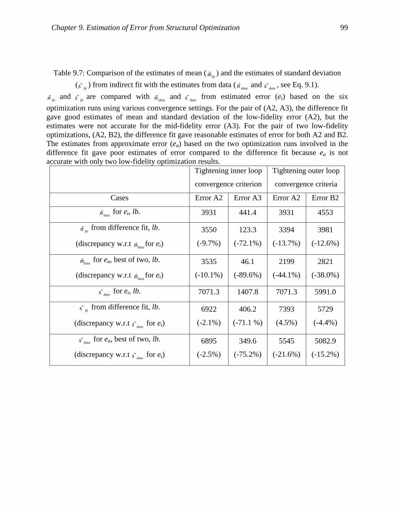
Chapter 9. Estimation of Error from Structural Optimization 99
Table 9.7: Comparison of the estimates of mean (fitµ ) and the estimates of standard deviation
(fitσ ) from indirect fit with the estimates from data (
dataµ and dataσ , see Eq. 9.1).
fitµ and fitσ are compared with
dataµ and dataσ from estimated error (et) based on the six
optimization runs using various convergence settings. For the pair of (A2, A3), the difference fit gave good estimates of mean and standard deviation of the low-fidelity error (A2), but the estimates were not accurate for the mid-fidelity error (A3). For the pair of two low-fidelity optimizations, (A2, B2), the difference fit gave reasonable estimates of error for both A2 and B2. The estimates from approximate error (ea) based on the two optimization runs involved in the difference fit gave poor estimates of error compared to the difference fit because ea is not accurate with only two low-fidelity optimization results.
Tightening inner loop
convergence criterion
Tightening outer loop
convergence criteria
Cases Error A2 Error A3 Error A2 Error B2
dataµ for et, lb. 3931 441.4 3931 4553
fitµ from difference fit, lb.
(discrepancy w.r.t dataµ for et)
3550
(-9.7%)
123.3
(-72.1%)
3394
(-13.7%)
3981
(-12.6%)
dataµ for ea, best of two, lb.
(discrepancy w.r.t dataµ for et)
3535
(-10.1%)
46.1
(-89.6%)
2199
(-44.1%)
2821
(-38.0%)
dataσ for et, lb. 7071.3 1407.8 7071.3 5991.0
fitσ from difference fit, lb.
(discrepancy w.r.t dataσ for et)
6922
(-2.1%)
406.2
(-71.1 %)
7393
(4.5%)
5729
(-4.4%)
dataσ for ea, best of two, lb.
(discrepancy w.r.t dataσ for et)
6895
(-2.5%)
349.6
(-75.2%)
5545
(-21.6%)
5082.9
(-15.2%)

Chapter 9. Estimation of Error from Structural Optimization 100
Minimize f(x)such that g(x) ≤ 0
FE Analysis
Generate approximationsf(x) and g(x) at xq
with move limits
x* = x q+1
kth iteration of MMFD, SQP or SLP
xq+1 = x qk
Converged forITRMOP times?
Converged?
Yes
YesNo
No
OUTER LOOP
INNER LOOP
Figure 9.1: Flow chart of GENESIS structural optimization software.

Chapter 9. Estimation of Error from Structural Optimization 101
design
Opt
imum
stru
ctur
alw
eigh
t(W
s)
5 10 15 2040000
60000
80000
100000
120000
Case A2Case A3Case A5
(a)
designO
ptim
umst
ruct
ural
wei
ght(
Ws)
5 10 15 2040000
60000
80000
100000
120000
Case B2Case B3Case B5
(b)
Figure 9.2: Optimum structural weight response along a design line for different GENESIS parameters, (a) Case A2, A3, and A5, (b) Case B2, B3, and B5.
Structural optimizations are performed for 21 HSCT configurations generated by linear interpolation between two extreme points in the five variable HSCT problem. Design 1 corresponds to (1, -1, 1, -1, 1) and design 21 corresponds to (-1, 1, -1, 1, -1) in a coded form of the HSCT configuration variables. The structural optimization resulted in two runs of large error with the default convergence parameters (A2). Tightening the outer loop convergence criteria (B2) from the default did not improve the structural optimization and resulted in a very noisy response of the optimum wing structural weight. By tightening the inner loop convergence criterion (A3, A5, B3 or B5), the structural optimizations are much more consistent and much less noisy.

Chapter 9. Estimation of Error from Structural Optimization 102
+
+
++
+
+
++
++
++
+
+
++
+
+
++
+
+++++++
++++
++
++++
++ +++
++
+++
++
++++
+
+
+
+ +++++
++
+
+
++++
+ +++
+
+++
+ +
+
+
+
+
+ +
+
+
+++
+
++
++
++ ++++
+
+ ++
+
++ ++ +
+
++
++
+ ++
+
+
+++
Ws, true (lb)
Err
orA
2(lb
)
0 100000 200000 3000000
5000
10000
15000
20000
25000
30000
35000
40000
45000
50000
(a) Case A2 (correlation = 0.5685).
+ +++
+
+
+ ++ +++
+
++ +
+
+++ + +++++++ + +++ ++
++++
++ +++
++
+++ +
+ +++++
++
+ +++++ + +++++++ + +++ ++++
+ ++++++ ++ +
+
+++++ + +++ +
+
++ ++ +++ +
+ +++
+
++
+
++ ++ ++
+
++
Ws, true (lb)
Err
orA
3(lb
)
0 100000 200000 3000000
2000
4000
6000
8000
10000
12000
14000
(b) Case A3 (correlation = 0.5089).
+
+
+
+
+
++ +
+ +
++ +
++
++
+
++ ++
++
++
+++ +
++
+
+
++
+
+
+
++
+
+
++++ + ++
++
+
++
+
+
++
+++
+
++
+
+
+
++++
+++
+
+
+
+
+
++
+
+
+
++
+
+
+++
+
++
+
+
+
+ ++++
+
+
+
+
+
++
+
++
+
++
+
++ +
++
+ ++
+
Ws, true (lb)
Err
orB
2(lb
)
0 100000 200000 3000000
5000
10000
15000
20000
25000
30000
35000
40000
45000
50000
(c) Case B2 (correlation =0.0844 ).
+ +++
+
++
+
++
++
+
+
+
+
+
++++
+
++++++ +
+
++++
+
+
+ +
+
+ +++ ++
+
+
+
+
+++++
+
++
+
+++++ + +++
+
+++ + +++ +++++ ++
++++
+
+
+
+
+
++
+
+
+
+
++ +
+++
+
+ +++
++ +
+
+
+
++
+
++
++
++
+++
Ws, true (lb)
Err
orB
3(lb
)
0 100000 200000 3000000
1000
2000
3000
4000
5000
6000
7000
8000
9000
10000
(d) Case B3 (correlation = 0.3588).
Figure 9.3: Plots of estimated error, et, versus estimated true Ws (absolute error).

Chapter 9. Estimation of Error from Structural Optimization 103
+
+
++
+
++
+
++
+++
+
++
+
+
++
+
++
++++++
++++
+++
++
++ +++
++
++ +
++
++
++
+
++
+ ++++++ +
+
+
++
++
+ +++
+
+++
++
+
+
+
+
+
+
+
+
+
++
+
+
+
++
++ ++++
+
+ ++
+
++ ++ +
+
+
+
++
+ ++
+
+
++
+
Ws, true (lb)
Err
orA
2(%
)
0 100000 200000 3000000
5
10
15
20
25
30
35
40
45
50
(a) Case A2 (correlation = 0.3210).
+ +++
+
+
+++ +++
+
+
+ +
+
+++ ++
++++++ + +++ +
+
+++
+
++
+++
+
+
++
+ ++ ++
+++
+ +
+ +++++ + +++++++
++
++ ++
+
+
+
++
++++
++ +
+
+++++
+ ++
+ +
+
++ ++ +
++
++ ++
+
+
++
+
+
+ ++
++
+
++
Ws, true (lb)
Err
orA
3(%
)0 100000 200000 300000
0
1
2
3
4
5
6
7
8
(b) Case A3 (correlation = 0.4326).
+
++
++
++ +
+ +
++
+++
+
+
+
++ + +++
+++
++ +
++
+
+
++
+
+
++
+
+
+
++
++ + +
+++
++
+
+
++
+
+++
+
++
+
+
+
++++
+++
+
+
+
+
+
++
+
+
+
+ +
+ +
+ ++
+++
+
+
+
+ +++
+ ++
+
+
+
+
+
+
+
+
+
++ +
++ +
+
+
+ ++
+
Ws, true (lb)
Err
orB
2(%
)
0 100000 200000 3000000
5
10
15
20
25
30
35
40
45
50
55
60
(c) Case B2 (correlation = -0.1321 ).
+ +++
+
++
+
+++
+
+
+
++
+
++++ +
++++++ +
+
++++
+
+
+ ++
+ +++ ++
+
+ + ++
+++++ + +
+
+++++ + +++
+
+++ + +++ +++++ ++
+++++
+
+
++
+++
+
+
+++ +
+++
++ +++
++ +
+
++
++
++
+
++
++ +++
Ws, true (lb)
Err
orB
3(%
)
0 100000 200000 3000000
5
10
15
(d) Case B3 (correlation = 0.0412).
Figure 9.4: Plots of estimated error, et, versus estimated true Ws (relative error).

Chapter 9. Estimation of Error from Structural Optimization 104
Sample size
Mea
nof
estim
ates
ofm
ean
ST
Dof
estim
ates
ofm
ean
50 100 1500
2000
4000
6000
8000
10000
0
2000
4000
6000
8000
10000
population meanmean of sample meanSTD of sample meanmean of fitted meanSTD of fitted mean
(a) µ .
Sample sizeM
ean
ofes
timat
esof
ST
D
ST
Dof
estim
ates
ofS
TD
50 100 1500
2000
4000
6000
8000
10000
12000
0
2000
4000
6000
8000
10000
population STDmean of sample STDSTD of sample STDmean of fitted STDSTD of fitted STD
(b) σ .
Figure 9.5: Comparison of µ and σ between Weibull fits and estimates from data according to the sample size.
For a given sample size ranging from 10 to 150, 50 sets of pseudo random numbers were generated from a Weibull distribution (α = 0.7682, β = 3915). The Weibull distribution has a population mean µ = 4572 lb. and standard deviation σ = 6023 lb., denoted as dashed lines. Then, µ and σ were estimated for each of the 50 sets by the two methods: estimates ( dataµ and
dataσ ) using Eq. 9.1 and fitting the Weibull model ( fitµ and fitσ ). The two methods were compared (solid lines correspond to the estimates using Eq. 9.1 and dash-dot lines correspond to the Weibull fit method) in terms of the mean and scatter of the estimates.

Chapter 9. Estimation of Error from Structural Optimization 105
+++++++++++++++++++++++++++++++++++++++++++++++++++++++++++++++++++++++++++++++++
+++++++++++++++++++++++++++
++++++
++++++ +
+ ++
+
+
Error A2 (Fit)
Err
orA
2(D
ata)
0 10000 20000 30000 40000 500000
10000
20000
30000
40000
50000
(a) Case A2.
+++++++++++++++++++++++++++++++++++++++++++++++++++++++++++++++++++++++++++++++++++++++++++++++++++++++++++
++++++++++++++
+ ++
+
+
Error A3 (Fit)
Err
orA
3(D
ata)
0 2000 4000 6000 8000 10000 120000
2000
4000
6000
8000
10000
12000
(b) Case A3.
+++++++++++++++++++++++++++++++++++++++++++++++++++++++
+++++++++++++++++++++++++++
++++++++++++++
++++++++++
++++++++
++++++ ++
+
+
++
Error B2 (Fit)
Err
orB
2(D
ata)
0 10000 20000 30000 400000
10000
20000
30000
40000
(c) Case B2.
++++++++++++++++++++++++++++++++++++++++++++++++++++++++++++++++++++++++++++++++++++++++++++
+++++++++++++
+++++++++
++++++ + +
+
+
+
+
Error B3 (Fit)
Err
orB
3(D
ata)
0 2000 4000 6000 8000 10000 120000
2000
4000
6000
8000
10000
12000
(d) Case B3.
Figure 9.6: Q-Q plots of Weibull fit for distribution of the estimated error. Points above the line indicate that the data is from a distribution with a heavier tail than the fit. For example, the point circled in Case A2 indicates that the probability of having an error greater than 20000 lb. in the fitted distribution is equal to the probability of exceeding an error of 24000 lb. in the data.

Chapter 9. Estimation of Error from Structural Optimization 106
Error(lb)
Fre
quen
cies
0 10000 20000 30000 40000 500000
10
20
30
40
50
60
70
DataExpected by direct fit
(a) Case A2.
Error(lb)
Fre
quen
cies
0 1000 2000 3000 40000
10
20
30
40
50
60
70
80
90
100
DataExpected by direct fit
(b) Case A3.
Error(lb)
Fre
quen
cies
0 10000 20000 30000 400000
10
20
30
40
DataExpected by direct fit
(c) Case B2.
Error(lb)
Fre
quen
cies
0 1000 2000 3000 40000
10
20
30
40
50
60
70
80
90
100
DataExpected by direct fit
(d) Case B3.
Figure 9.7: Comparison of histograms of et and direct fits of Weibull model.
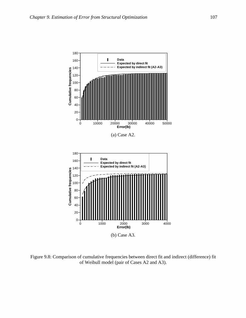
Chapter 9. Estimation of Error from Structural Optimization 107
Error(lb)
Cum
ulat
ive
freq
uenc
ies
0 10000 20000 30000 40000 500000
20
40
60
80
100
120
140
160
180
DataExpected by direct fitExpected by indirect fit (A2-A3)
(a) Case A2.
Error(lb)
Cum
ulat
ive
freq
uenc
ies
0 1000 2000 3000 40000
20
40
60
80
100
120
140
160
180
DataExpected by direct fitExpected by indirect fit (A2-A3)
(b) Case A3.
Figure 9.8: Comparison of cumulative frequencies between direct fit and indirect (difference) fit of Weibull model (pair of Cases A2 and A3).
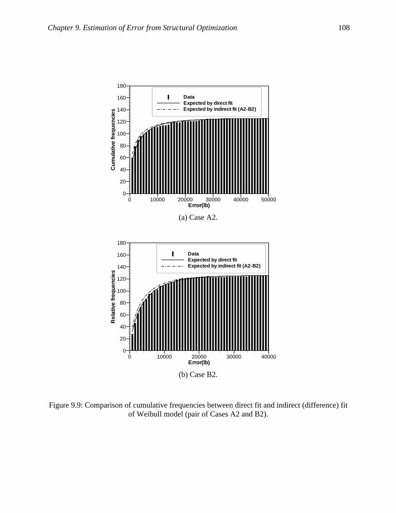
Chapter 9. Estimation of Error from Structural Optimization 108
Error(lb)
Cum
ulat
ive
freq
uenc
ies
0 10000 20000 30000 40000 500000
20
40
60
80
100
120
140
160
180
DataExpected by direct fitExpected by indirect fit (A2-B2)
(a) Case A2.
Error(lb)
Rel
ativ
efr
eque
ncie
s
0 10000 20000 30000 400000
20
40
60
80
100
120
140
160
180
DataExpected by direct fitExpected by indirect fit (A2-B2)
(b) Case B2.
Figure 9.9: Comparison of cumulative frequencies between direct fit and indirect (difference) fit of Weibull model (pair of Cases A2 and B2).

Chapter 9. Estimation of Error from Structural Optimization 109
Sample size
Mea
nof
estim
ates
ofm
ean
ST
Dof
estim
ates
ofm
ean
30 40 50 60 70 80 90 100 110 120 1300
1000
2000
3000
4000
5000
6000
7000
8000
9000
10000
0
1000
2000
3000
4000
5000
Mean of fitted mean (A2)STD of fitted mean (A2)Mean of fitted mean (B2)STD of fitted mean (B2)
(a) µ .
Sample size
Mea
nof
estim
ates
ofS
TD
ST
Dof
estim
ates
ofS
TD
30 40 50 60 70 80 90 100 110 120 1300
2000
4000
6000
8000
10000
12000
0
2000
4000
6000
8000
10000
12000
Mean of fitted STD (A2)STD of fitted STD (A2)Mean of fitted STD (B2)STD of fitted STD (B2)
(b) σ .
Figure 9.10: µ and σ of the difference fit for the pair of (A2, B2) for various sample sizes. For each given sample size ranging from 30 to 130, 50 sets of data were generated from the 126 data with replacement. One can observe that µ and σ have large scatter at small sample sizes particularly for A2, and stabilize as the sample size increases.

110
Chapter 10 Detection and Repair of Poorly
Converged Structural Optimization Runs
In the previous chapter we used probabilistic models to estimate the average error from
structural optimization of the HSCT. In this chapter we will address the problem of structural
optimizations with large error, outliers. In Chapter 8, robust regression techniques were used to
identify outliers in optimization runs for the Rosenbrock test function, and we showed that
outlier repair greatly improved the quality of the optimum of the response surface (RS) model
based on the optimization data.
The structural optimization was performed to build a response surface approximation for
the wing bending material weight of an HSCT. If we use low-fidelity data contaminated with
outliers such as Case A2 of Section 9.1, the RS fit can be inaccurate because the least squares fit
is not robust, and eventually it may increase uncertainty in the system level design of the HSCT.
One obvious solution is to use high-fidelity data, such as Case A5 of Section 9.1, to get an
accurate fit. However, high-fidelity optimizations may be much more expensive than low-fidelity
cases. We noted that high-fidelity structural optimization requires more than twice the CPU time
than low-fidelity cases. Moreover, it is possible that the high-fidelity simulation is not available
because we do not know how to improve the low-fidelity simulation. Hence, it may be more
efficient to repair only the identified outliers by high-fidelity simulations rather than doing high-
fidelity simulations from the beginning, when high-fidelity runs are much more expensive than
lower fidelity runs.
10.1 IRLS Procedures for the Optimization Error: Symmetric and
Non-symmetric Weighting Functions
The IRLS procedure to identify poor optimizations was applied to the lower-fidelity
HSCT structural optimization data, Case A2 and Case B2 (see Section 9.1). The SAS [90]
statistical software was used to do the IRLS fit. See Appendix G for an example of the SAS input
file for IRLS. A full quadratic polynomial model of a five dimensional design space was used for

Chapter 10. Detection and Repair of Poorly Converged Structural Optimization Runs 111
the RS fit. The one-sidedness of the optimization error due to incomplete convergence led us to
the nonsymmetric IRLS (NIRLS) using a nonsymmetic weighting function, which was compared
to regular IRLS. The IRLS results depend on the shape of the weighting function. The tuning
constant B acts like a threshold for outlier detection (see Table 6.1). A smaller B leads to a more
aggressive outlier search; the allowable region around the RS for good points becomes narrower,
and more points will be declared outliers. Two different values of the tuning constant B were
tried. B = 1.0, the same value as for the Rosenbrock test function in Section 8.4, corresponds to
an aggressive outlier search, while B = 1.9 corresponds to a moderate outlier search. For NIRLS,
the tuning constant H controlling the weighting function for negative residuals was kept at 1.0,
while B that controls the weighting function for the positive residuals was changed (see Table
6.1).
For the detected outlier points that have a weighting of less than 0.01, we corrected them
by the estimated true Ws, which was calculated by taking the best of the two high-fidelity Cases
(A5 and B5) and two low-fidelity cases (A2 and B2). The contribution from the mid-fidelity data
(B3 and A3) to estimating true Ws would be small. The averages of the estimated errors are
shown in Table 10.1, which shows almost the same magnitude compared to the results of Table
9.2 that utilized all of the six cases.
10.2 Results of Outlier Detection and Repair
Table 10.2 presents a summary of the outlier detection and correction results for Case A2
with IRLS and NIRLS. In the RS fit, we removed 11 points of extraordinarily heavy designs (Ws
greater than 150000 lb., which is about triple the usual optimum designs) from 126 data points
and used only 115 points, because we did not want to consider unreasonable designs. This
approach of excluding design points with unreasonable results is known as the reasonable design
space approach [8]. The identified outliers were repaired by the estimated true Ws. To assess the
success in detection, all 115 points were also repaired, and the results are shown in the last row
in Table 10.2.
With a tuning constant B = 1.9, IRLS and NIRLS identified two different sets of 21 data
points as outliers. Twelve out of the 21 points were common. The error in the outliers is
calculated by comparing Ws(A2) to the repaired value. For comparison, we also repaired points

Chapter 10. Detection and Repair of Poorly Converged Structural Optimization Runs 112
not flagged as outliers. For IRLS, the average correction was 7391 lb. for outliers compared to
1516 lb. for inliers. NIRLS did a better job in finding outliers; the average correction was 8627
lb. for outliers and 1240 lb. for inliers. The ratio between the average corrections of Ws for
outliers and inliers can be considered as a measure of the success of outlier detection. For NIRLS
the ratio was 6.96 compared to 4.88 of IRLS.
Figure 10.1 shows the estimated error (i.e., Ws repair) of both of the detected outliers and
inliers versus w, the weighting in IRLS. Big outliers are of particular concern. We defined big
outliers as those showing 10% or greater error. Eleven out of 115 points satisfy this criterion, and
ten out of these were detected by all approaches listed in Table 10.2. Figure 10.1(a) shows that
IRLS left many moderate outliers undetected. By more aggressive detection with B = 1.0, IRLS
declared 40 points as outliers, and Figure 10.1(b) shows that more of the moderate outliers were
detected by decreasing B. Again, NIRLS was more effective in discriminating outliers from
inliers with a ratio of errors of 5.87 compared to 4.27 for IRLS. The aggressive outlier search
with B = 1.0 does find more outliers. However, it declares more points as outliers and the
computational advantage of repairing only outliers may be reduced. For example, the number of
outliers declared by NIRLS increased from 21 with B = 1.9 to 41 with B = 1.0. Taking the mean
CPU hour of Case A2 as a single unit, our efforts to repair Case A2, requiring GENESIS runs of
Cases A5, B2, and B5, costs about extra 4.6 units of CPU hour. Compared to obtaining accurate
Ws for all data points using Cases A2, A5, B2, and B5, NIRLS repair costs about 33% and 47%
CPU hours for B = 1.9 and B = 1.0, respectively.
Table 10.3 and Figure 10.2 show results for Case B2. Again, nine data points of
excessively heavy designs were excluded from the experimental design. There were 22 big
outliers in the remaining 117 data points, indicating a higher level of noise than Case A2. The
advantage of NIRLS over IRLS is clearly demonstrated by comparing the results when B = 1.0.
NIRLS successfully detected all of the 22 big outliers and many moderate ones, while IRLS
missed six of the big outliers. With more noise, the ratio of correction of Ws for outliers and
inliers is 5.97 for NIRLS compared to 2.67 for IRLS with B = 1.0, indicating that NIRLS is more
successful in homing in on points with large errors. Again, the aggressive outlier search detects
more outliers but there is increased computational cost. Taking the mean CPU hour of Case B2
as a single unit, our efforts to repair Case B2, requiring GENESIS runs of Cases A2, A5, and B5,
costs about six extra units of CPU hour. Compared to obtaining accurate Ws for all data points

Chapter 10. Detection and Repair of Poorly Converged Structural Optimization Runs 113
using Cases A2, A5, B2, and B5, NIRLS repair costs about 36% and 52% of CPU hour for B =
1.9 and B = 1.0, respectively.
Taken together, the results of Case A and Case B indicate that the IRLS procedures are
useful for detecting points with large optimization errors, and that the NIRLS procedures are
more reliable in this task, especially under conditions of greater noise.
10.3 Advantage of Outlier Repair over Exclusion
The IRLS procedure in itself achieves a better fit than the least squares by down-
weighting outlier points and excluding them from the fit. However, removing the outliers can
result in a poor approximation in the region where these outliers are located [45]. Repairing these
outliers, on the other hand, does not suffer from this problem. Figure 10.3 compares the Ws
prediction by RS approximations along a design line connecting two detected outliers. It shows
that the least squares results based on repaired data are better than IRLS without repair because
the latter excluded those outliers from the fit. Therefore, it was decided to use the least squares
fit to the repaired data to obtain improved RS approximations.
10.4 Improvement of Wing Structural Weight RS Approximations
Using Repaired Data A full quadratic RS model was fit to the original and repaired data of Case A2 using the
least squares fit, and the accuracy measures are shown in the last two columns of Table 10.2.
Before repair, the root mean square error (RMSE) was 6.0% of the mean Ws, and this was
reduced to 3.2% by IRLS repair. Although more of the moderate outliers were repaired by
NIRLS than IRLS, further improvement of the fit by NIRLS was small; the RMSE was 3.1%. It
implies that the gain of outlier repair in terms of fit is saturated with IRLS. In fact the RMSE was
slightly increased to 3.3% with full repair. That is because IRLS/NIRLS procedure identifies
only offending data points against the fit, while full repair may move away non-offending points
from the fit. Besides, this problem of the full repair may be attributed to that the repaired Ws
response is not perfectly smooth as seen in Figure 3.4. Overall, about the half of the RMSE

Chapter 10. Detection and Repair of Poorly Converged Structural Optimization Runs 114
before outlier repair is due to the error from incomplete convergence, and the rest may be
attributed to the modeling deficiency of the quadratic model.
For Case B2 in Table 10.3, the RMSE of the quadratic RS fits on Ws(B2) was reduced
from 8.7% to 4.1% by IRLS repair, and reduced further to 3.2% by NIRLS repair. Note that six
additional big outliers were repaired with NIRLS. Figure 10.4 compares the RS approximations
before and after repair along the same HSCT designs used in Figure 9.2. The RS fit based on the
uncorrected Ws (B2) over-predicted the response in the middle of the plot. For B = 1.9, as shown
in Figure 10.4(a), the RS approximation based on data repaired by IRLS improved. Note that the
RS approximation from NIRLS repair lies almost on top of that of IRLS. However, Figure
10.4(b) indicates that NIRLS repair was slightly better than IRLS with B = 1.0 at the right region
of the plot. These observations are in agreement with the results of RMSE of Table 10.3. In
terms of accuracy of Ws RS fits, outlier repair by IRLS improved the RS approximations
substantially, and further gain by NIRLS repair was relatively small.
10.5 HSCT Configuration Optimization Using Improved Wb RS
Approximations
We performed HSCT configuration optimizations using the quadratic Wb RS fits obtained
in the previous section. The effects of improvements of RS approximations by outlier repair on
optimum HSCT designs were investigated. Note that Wb RS approximations were obtained by
multiplying the Ws response surface approximations by a factor of 0.7 because we assumed that
Wb was 70% of Ws. Table 10.4 contains the initial and optimal designs according to the RS
models used. The initial design point was the center of the design box except that the fuel weight
was increased to 430000 lb. to satisfy the range constraint at the beginning of the configuration
optimization. The RS fit based on Case B2 data without outlier repair was first used to find the
optimal HSCT configuration, called optimum O. Then, configuration optimizations starting from
optimum O are performed using RS fits based on repaired data: IRLS repair with B = 1.9 (RSI),
NIRLS repair with B = 1.9 (RSN), and full repair (RSF). The corresponding optimal HSCT
designs were labeled as optimum I, N, and F, respectively. At the initial design, the estimated
true Wb was 48633 lb. but the RS approximation without outlier repair, RSO, over-predicted Wb
Chapter 10. Detection and Repair of Poorly Converged Structural Optimization Runs 115
with 12.0% error. By repairing outliers, the error was reduced to 7.4%, 5.1%, and 1.8% for RSI,
RSN, and RSF, respectively.
Comparing the RS prediction for a given optimum design (column), we observe that the
predicted Wb’s decrease along RSO, RSI, RSN, and RSF. It is seen that the original RS
approximation, RSO, has positive errors while RS fits with repair tend to have negative errors,
which increase in magnitude along RSI, RSN, and RSF. For example, at optimum O, RSO has a
positive error of 9.1%, but the errors became more negative along RSI, RSN, and RSF with –4.9%,
-6.8%, and –7.3% errors, respectively. The same trend is observed for optima I, N, and F. This
may be attributed to over-optimism of the optimizer; optimizers tend to exploit regions where the
fits are erroneously optimistic, and converge to designs for which the RS approximations under-
predict the response. By intensive outlier repair such as NIRLS or full repair, Wb estimates by the
RS fits are lowered, and then any exploitation of weakness of the RS approximations by the
optimizer is fully experienced at the optimum.
Therefore, a moderate outlier search such as IRLS may be conservative in the terms of
the configuration optimization. It has a protective margin against over-optimism of the optimizer
because the moderately corrected RS fit would slightly over-predict the structural weight over
much of the design space. The errors of the RS approximation at optima support this conjecture.
For optimum O, RSO over-predicted Wb with 9.1% error. For optimum I of IRLS repair, the error
of RSI was only 0.4%, although RSI cannot be expected to show such accuracy in general because
for other optima, RSI has errors around –5%. For optimum N of NIRLS repair, RSN under-
predicted the Wb with –3.2% error. Furthermore, for optimum F of full repair, RSF has –7.5%
error. The take-off gross weight of the optima decreases as Wb predicted by RS approximations
decreases with more outliers repaired.
Table 10.4 contains the configuration variables at the optima, and the shape of the
planform and airfoil are compared in Figure 10.5 for initial and optimal designs. Comparing
optimum O, I, N, and F, they are very similar with the only significance being the fuel weight
(v5), which decreases as a compensation of the decrease in predicted Wb. Accordingly, the
objective function, WTOGW, decreases along optimum O, I, N, and F, and the range constraint was
active for all the optima.

Chapter 10. Detection and Repair of Poorly Converged Structural Optimization Runs 116
Table 10.1: Performance of structural optimization for various GENESIS parameter settings. Case A2 Case A5 Case B2 Case B5
Number of points for which the best Ws
was achieved out of 126 points 0 65 0 61
Mean of the estimated errors by taking
the best of four runs as true Ws
(percentage of mean Ws)
3925 lb.
(4.85%)
155.8 lb.
(0.193%)
4547 lb.
(5.62%)
26.8 lb.
(0.033%)

Chapter 10. Detection and Repair of Poorly Converged Structural Optimization Runs 117
Table 10.2: Results of outlier repair for Case A2.
B
Number of
outliers
a/b/c*
Mean of repair
on
outliers(lb)†
Mean of repair
on inliers(lb)‡
Ratio of mean
repair on OL to
IL
mean Ws R2
RMSE in lb.
(% to the
mean Ws)
Before
repair NA NA NA NA NA 74795 0.9652
4520
(6.0%)
IRLS
repair 1.9 21/10/11 7391 1516 4.88 73445 0.9836
2944
(4.0%)
NIRLS
repair 1.9 21/10/11 8627 1240 6.96 73220 0.9878
2484
(3.4%)
IRLS
repair 1.0 40/10/11 5172 1211 4.27 72996 0.9891
2367
(3.2%)
NIRLS
repair 1.0 41/10/11 5555 946 5.87 72815 0.9900
2252
(3.1%)
Full
repair§ NA NA NA NA NA 72206 0.9885
2388
(3.3%)
*: a ~ Number of detected outliers b ~ Number of big outliers detected (estimated error is greater than 10%) c ~ Total number of big outliers out of the 115 data points (estimated error is greater than 10%) †: (Sum of Ws repair on outliers)/a ‡: (Sum of Ws repair on data points other than outliers)/(Total number of points - a) §: All 115 points repaired

Chapter 10. Detection and Repair of Poorly Converged Structural Optimization Runs 118
Table 10.3: Results of outlier repair for Case B2.
B
Number of
outliers
a/b/c*
Mean of repair
on
outliers(lb)†
Mean of repair
on inliers(lb)‡
Ratio of mean
repair on OL to
IL
mean Ws R2
RMSE in lb.
(% to the
mean Ws)
Before
repair NA NA NA NA NA 77701 0.9297
6755
(8.7%)
IRLS
repair 1.9 27/11/22 8694 3314 2.62 75695 0.9769
3527
(4.7%)
NIRLS
repair 1.9 29/19/22 11379 2307 4.93 74881 0.9824
3042
(4.1%)
IRLS
repair 1.0 49/16/22 7158 2680 2.67 74703 0.9828
3052
(4.1%)
NIRLS
repair 1.0 52/22/22 8476 1419 5.97 73934 0.9902
2335
(3.2%)
Full
repair§ NA NA NA NA NA 73146 0.9879
2578
(3.5%)
*: a ~ Number of detected outliers b ~ Number of big outliers detected (estimated error is greater than 10%) c ~ Total number of big outliers out of the 117 data points (estimated error is greater than 10%) †: (Sum of Ws repair on outliers)/a ‡: (Sum of Ws repair on data points other than outliers)/(Total number of points - a) §: All 117 points repaired
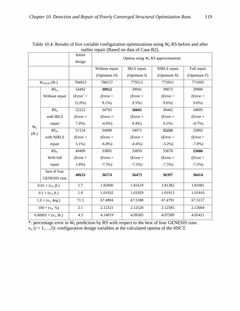
Chapter 10. Detection and Repair of Poorly Converged Structural Optimization Runs 119
Table 10.4: Results of five variable configuration optimizations using Wb RS before and after outlier repair (Based on data of Case B2).
Initial
design Optima using Wb RS approximations
Without repair
(Optimum O)
IRLS repair
(Optimum I)
NIRLS repair
(Optimum N)
Full repair
(Optimum F)
WTOGW (lb.) 784923 788157 779512 775931 771693
RSo,
Without repair
54492
(Error* =
12.0%)
39912
(Error =
9.1%)
39941
(Error =
9.5%)
39873
(Error =
9.6%)
39900
(Error =
9.6%)
RSI,
with IRLS
repair
52222
(Error =
7.4%)
34792
(Error =
-4.9%)
36601
(Error =
0.4%)
36442
(Error =
0.1%)
34695
(Error =
-4.7%)
RSN,
with NIRLS
repair
51124
(Error =
5.1%)
34088
(Error =
-6.8%)
34071
(Error =
-6.6%)
35235
(Error =
-3.2%)
33892
(Error =
-7.0%)
RSF,
With full
repair
49499
(Error =
1.8%)
33895
(Error =
-7.3%)
33859
(Error =
-7.2%)
33678
(Error =
-7.5%)
33686
(Error =
-7.5%)
Wb
(lb.)
best of four
GENESIS runs 48633 36574 36473 36397 36414
0.01 × (v1, ft.) 1.7 1.82000 1.81619 1.81382 1.81081
0.1 × (v2, ft.) 1.0 1.01932 1.01929 1.01913 1.01910
1.0 × (v3, deg.) 71.5 67.4904 67.5588 67.4791 67.5157
100 × (v4, %) 2.1 2.12321 2.12528 2.12585 2.12664
0.00001 × (v5, lb.) 4.3 4.14019 4.09583 4.07589 4.05421
*: percentage error in Wb prediction by RS with respect to the best of four GENESIS runs. vi, (i = 1,…,5): configuration design variables at the calculated optima of the HSCT.

Chapter 10. Detection and Repair of Poorly Converged Structural Optimization Runs 120
Weighting, w
Est
imat
eder
ror
ofW
s(%
)
0.00 0.25 0.50 0.75 1.000
10
20
30
40
50
OutlierInlier
(a) IRLS, B = 1.9.
Weighting, wE
stim
ated
erro
rof
Ws
(%)
0.00 0.25 0.50 0.75 1.000
10
20
30
40
50
OutlierInlier
(b) IRLS, B = 1.0.
Weighting, w
Est
imat
eder
ror
ofW
s(%
)
0.00 0.25 0.50 0.75 1.000
10
20
30
40
50
OutlierInlier
(c) NIRLS, B = 1.9.
Weighting, w
Est
imat
eder
ror
ofW
s(%
)
0.00 0.25 0.50 0.75 1.000
10
20
30
40
50
OutlierInlier
(d) NIRLS, B = 1.0.
Figure 10.1: Estimated error for the detected outliers and inliers for Case A2.
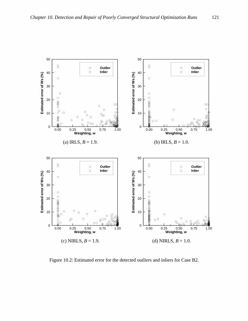
Chapter 10. Detection and Repair of Poorly Converged Structural Optimization Runs 121
Weighting, w
Est
imat
eder
ror
ofW
s(%
)
0.00 0.25 0.50 0.75 1.000
10
20
30
40
50
OutlierInlier
(a) IRLS, B = 1.9.
Weighting, wE
stim
ated
erro
rof
Ws
(%)
0.00 0.25 0.50 0.75 1.000
10
20
30
40
50
OutlierInlier
(b) IRLS, B = 1.0.
Weighting, w
Est
imat
eder
ror
ofW
s(%
)
0.00 0.25 0.50 0.75 1.000
10
20
30
40
50
OutlierInlier
(c) NIRLS, B = 1.9.
Weighting, w
Est
imat
eder
ror
ofW
s(%
)
0.00 0.25 0.50 0.75 1.000
10
20
30
40
50
OutlierInlier
(d) NIRLS, B = 1.0.
Figure 10.2: Estimated error for the detected outliers and inliers for Case B2.
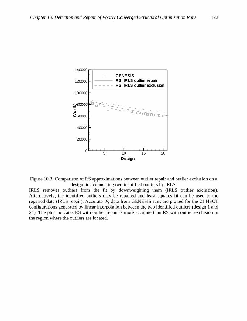
Chapter 10. Detection and Repair of Poorly Converged Structural Optimization Runs 122
Design
Ws
(lb)
5 10 15 200
20000
40000
60000
80000
100000
120000
140000
GENESISRS: IRLS outlier repairRS: IRLS outlier exclusion
Figure 10.3: Comparison of RS approximations between outlier repair and outlier exclusion on a design line connecting two identified outliers by IRLS.
IRLS removes outliers from the fit by downweighting them (IRLS outlier exclusion). Alternatively, the identified outliers may be repaired and least squares fit can be used to the repaired data (IRLS repair). Accurate Ws data from GENESIS runs are plotted for the 21 HSCT configurations generated by linear interpolation between the two identified outliers (design 1 and 21). The plot indicates RS with outlier repair is more accurate than RS with outlier exclusion in the region where the outliers are located.
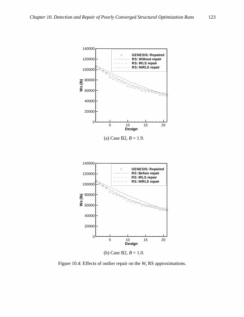
Chapter 10. Detection and Repair of Poorly Converged Structural Optimization Runs 123
Design
Ws
(lb)
5 10 15 200
20000
40000
60000
80000
100000
120000
140000
GENESIS: RepairedRS: Without repairRS: IRLS repairRS: NIRLS repair
(a) Case B2, B = 1.9.
Design
Ws
(lb)
5 10 15 200
20000
40000
60000
80000
100000
120000
140000
GENESIS: RepairedRS: Before repairRS: IRLS repairRS: NIRLS repair
(b) Case B2, B = 1.0.
Figure 10.4: Effects of outlier repair on the Ws RS approximations.

Chapter 10. Detection and Repair of Poorly Converged Structural Optimization Runs 124
Inital Design
Optimum O (Wb RS without repair)
(a) Initial design and original optimum
Optimum O (Wb RS without repair)
Optimum I (Wb RS with IRLS repair)
(b) IRLS repair.
Optimum O (Wb RS without repair)
Optimum N (Wb RS with NIRLS repair)
(c) NIRLS repair.
Optimum O (Wb RS without repair)
Optimum F (Wb RS with full repair)
(d) Full repair.
Figure 10.5: Comparison of optimum designs using Wb RS approximations without and with outlier repair (based on data of Case B2).

125
Chapter 11 Conclusions
The goal of this work was to apply statistical techniques to estimate and reduce errors of
the computational simulations used in the design of an HSCT. First, discretization error from a
supersonic panel method, WINGDES, was considered. Second, errors in wing structural weight
calculated from a structural optimization procedure using GENESIS were analyzed along with
the Rosenbrock test problem. The noisy optimization errors were modeled via probability
distributions. A robust regression technique, IRLS, was used to identify optimization runs with
large errors and to improve the RS fit on the optimization data.
A grid convergence study showed that CL calculated from WINGDES was subject to
discretization error that converged like h0.5. Richardson extrapolation was not accurate because it
magnified the noise in CL data. A RS model using several mesh sizes reduced the noise problem
associated with the Richardson extrapolation. In addition, the RS approach was compared to
posterior response surface fit to Richardson extrapolation, and was shown to be efficient in
estimating the discretization error by using carefully selected experimental designs.
Probabilistic models were applied to optimization errors due to incomplete convergence.
The Weibull model was successfully fit to the optimization errors for the Rosenbrock test
function and structural optimization of the HSCT. The minimum sample size for a reliable
estimate of average error was around 50. An indirect approach using differences between two
optimization results was proposed. The indirect fit enabled us to estimate the average errors of
low-fidelity optimizations without performing high-fidelity optimizations that can be expensive.
The results demonstrated the usefulness of the probabilistic model of the optimization error. As a
result, we obtained a data-driven probability model of the simulation errors, which can be easily
utilized in robust design studies.
A robust regression technique, M-estimation implemented by the IRLS algorithm, was
applied to the Rosenbrock problem to identify optimization runs with large errors, outliers. We
elected to repair the outliers by performing higher fidelity optimization runs, because excluding
data points may reduce the accuracy of the RS model. For the Rosenbrock problem, outlier repair
efforts substantially improved the quality of the optimum of the RS model. Then we devised
nonsymmetric IRLS (NIRLS) with a nonsymmetric weighting function, to utilize the tendency of

Chapter 11. Conclusions 126
one-sidedness of the optimization errors. It was shown that NIRLS was more reliable than IRLS
in identifying outliers from optimization results.
Structural optimization data with large errors resulted in inaccurate RS models of the
wing bending material weight (Wb). The IRLS/NIRLS procedure was also applied to identify and
repair the outliers. Again, NIRLS was more effective than IRLS in identifying outliers. In terms
of RS fit, IRLS repair substantially improved the accuracy of the RS model, while further
improvements by NIRLS were relatively small. HSCT configuration optimizations were
performed using Wb RS models before and after outlier repair. The results indicated that the
system optimizer exploited the modeling error of the RS model, and the moderate outlier repair
of IRLS was a conservative choice compared to NIRLS repair in the HSCT design problem.

127
Bibliography [1] Sobieszczanski-Sobieski, J., “Multidisciplinary Design Optimization (MDO) methods: their
synergy with computer technology in the design process,” Aeronautical Journal, Vol. 103,
No. 1026, 1999, pp. 373-382.
[2] Mavris, D. N., DeLaurentis, D. A., Bandte, O., and Hale, M. A., “A Stochastic Approach to
Multi-disciplinary Aircraft Analysis and Design,” AIAA Paper 98-0912, 36th Aerospace
Science Meeting & Exhibit, Reno, NV, January, 1998.
[3] Sobieszczanski-Sobieski, J. and Haftka, R. T., “Multidisciplinary Aerospace Design
Optimization: Survey of Recent Developments,” Structural Optimization, Vol. 14, No. 1,
1997, pp. 1-23.
[4] Knill, D. L., Giunta, A. A., Baker, C. A., Grossman, B., Mason, W. H., Haftka, R. T., and
Watson, L. T., “Response Surface Models Combining Linear and Euler Aerodynamics for
Supersonic Transport Design,” Journal of Aircraft, Vol. 36, No. 1, 1999, pp. 75-86.
[5] Raveh, D. E., Levy, Y., and Karpel, M., “Aircraft Aeroelastic Analysis and Design Using
CFD-Based Unsteady Loads,” AIAA Paper 2000-1325, 41st AIAA/ASME/ASCE/AHS/ASC
Structures, Structural Dynamics, & Materials Conference, Atlanta, GA, April, 2000.
[6] Sobieszczanski-Sobieski, J., Kodiyalam, S., and Yang, R., “Optimization of Car Body under
Constraints of Noise, Vibration, and Harness (HVN), and Crash,” AIAA Paper 2000-1521,
41st AIAA/ASME/ASCE/AHS/ASC Structures, Structural Dynamics, & Materials
Conference, Atlanta, GA, April, 2000.
[7] Balabanov, V., Kaufman, M., Knill, D. L., Haim, D., Golovidov, O., Giunta, A., A., Haftka,
R. T., Grossman, B., Mason, W. H., and Watson, L. T., “Dependence of Optimal Structural
Weight on Aerodynamic Shape for a High Speed Civil Transport,” AIAA Paper 1996-4046,
6th AIAA/NASA/ISSMO Symposium on Multidisciplinary Analysis and Optimization,
Bellevue, WA, September, 1996.
[8] Balabanov, V., Giunta, A. A., Golovidov, O., Grossman, B., Mason, W. H., Watson, L. T.,
and Haftka, R. T., “Reasonable Design Space Approach to Response Surface
Approximation,” Journal of Aircraft, Vol. 36, 1999, pp. 308-315.

Bibliography 128
[9] Roache, P. J., Verification and Validation in Computational Science and Engineering,
Hermosa Publishers, Albuquerque, NM, 1998.
[10] Giunta, A. A., Dudley, J. M., Narducci, R., Grossman, B., Haftka, R. T., Mason, W. H., and
Watson, L. T., “Noisy Aerodynamics Response and Smooth Approximations in HSCT
Design,” AIAA Paper 94-4376, 5th AIAA/USAF/NASA/ISSMO Symposium on
Multidisciplinary Analysis and Optimization, Panama City, FL, September, 1994.
[11] Venter, G., Haftka, R. T., and Starnes, J. H., “Construction of Response Surfaces for Design
Optimization Applications,” AIAA Paper 96-4040, 6th AIAA/NASA/ISSMO Symposium on
Multidisciplinary Analysis and Optimization, Bellevue, WA, September, 1996.
[12] Mehta, U. B., “Guide to Credible Computer Simulations of Fluid Flows,” Journal of
Propulsion and Power, Vol. 12, No. 5, 1996, pp. 940-948.
[13] Chen, W., Allen, J. K., Mistree, F., and Tsui, K. L., “A Procedure for Robust Design:
Minimizing Variations Caused by Noise Factors and Control Factors,” Journal of
Mechanical Design, Vol. 118, No. 4, 1996, pp. 478-485.
[14] Mavris, D. N., Bandte, O., and Schrage, D. P., “Application of Probabilistic Methods for the
Determination of Probabilistic Methods for the Determination of an Economically Robust
HSCT Configuration,” AIAA Paper 96-4090, 6th AIAA/NASA/ISSMO, Symposium on
Multidisciplinary Analysis and Optimization, Bellevue, WA, September, 1996.
[15] Gantois, K. and Morris, A. J., “Incorporation of Manufacturing Information into an MDO
environment,” Aeronautical Journal, Vol. 103, No. 1026, 1999, pp. 383-388.
[16] Mavris, D. N., Bandte, O., and DeLaurentis, D. A., “Robust Design Simulation: A
Probabilistic Approach to Multidisciplinary Design,” Journal of Aircraft, Vol. 36, No. 1,
1999, pp. 298-307.
[17] Venter, G. and Haftka, R. T., “Using Response Surface Approximations in Fuzzy Set Based
Design Optimization,” Structural Optimization, Vol. 18, No. 4, 1999, pp. 218-227.
[18] Chen, S., Nikolaidis, E., Cudney, H. H., Rosca, R., and Haftka. R.T., “Comparison of
Probabilistic and Fuzzy Set Methods for Designing under Uncertainty,” AIAA Paper 99-
1579, 40th AIAA/ASME/ASCE/AHS/ASC Structures, Structural Dynamics, & Materials
Conference, St. Louis, MO, April, 1999.

Bibliography 129
[19] Lombardi, M. and Haftka, R. T., “Anti-Optimization Technique for Structural Design under
Uncertainties,” Computer Methods in Applied Mechanics and Engineering, Vol. 157, No. 1,
1998, pp. 19-31.
[20] Chen, R. and Ward, A. C., “The RANGE Family of Propagation Operations for Intervals on
Simultaneous Linear Equations,” Artificial Intelligence for Engineering Design, Analysis and
Manufacturing, Vol. 9, No. 3, 1995, pp. 183-196.
[21] Hoover, S. V. and Perry, R. F., Simulation: A Problem-Solving Approach, Addison Wesley
Longman, Reading, MA, 1989.
[22] Stein, M., “Large Sample Properties of Simulations Using Latin Hypercube Sampling,”
Technometrics, Vol. 29, No. 2, 1987, pp. 143-151.
[23] Phadke, M. S., Quality Engineering using Robust Design, Prentice-Hall, Englewood Cliffs,
NJ, 1989.
[24] Southwest Research Institute, FPI User’s and Theoretical Manual, San Antonio, TX, 1995.
[25] Mavris, D. N. and Bandte, O., “A Probabilistic Approach to Multivariate Constrained Robust
Design Simulation,” AIAA Paper 97-5508, AIAA and SAE 1997 World Aviation Congress,
Anaheim, CA, October, 1997.
[26] Celik, I. and Zhang, W., “Calculation of Numerical Uncertainty Using Richardson
Extrapolation: Application to Some Simple Turbulent Flow Calculations,” Journal of Fluids
Engineering, Transactions of ASME, Vol. 117, No. 3, 1995, pp. 439-435.
[27] Coleman, H. W. and Stern, F., “Uncertainties and CFD Code Validation,” Journal of Fluids
Engineering, Vol. 119, No. 4, 1997, pp. 795-803.
[28] Anderson, E. L. and Hattis, D., “Uncertainty and Variability,” Risk Analysis, Vol. 19, No. 1,
1999, pp. 47-49.
[29] Antonsson, E. K. and Otto, K. N., “Imprecision in Engineering Design,” ASME Journal of
Mechanical Engineering, Vol. 117B, 1995, pp. 25-32.
[30] French, S., “Uncertainty and Imprecision: Modelling and Analysis,” Journal of the
Operational Research Society, Vol. 46, No. 1, 1995, pp. 70-79.
[31] Coleman, H. W. and Steele, W. G., Jr., Experimentation and Uncertainty Analysis for
Engineers, 1st Ed., John Wiley & Sons, New York, 1989.

Bibliography 130
[32] Gu, X., Renaud, J. E., and Batill, S. M., “An Investigation of Multidisciplinary Design
Subject to Uncertainty,” AIAA Paper 98-4747, 7th AIAA/NASA/USAF/ISSMO Symposium
on Multidisciplinary Analysis and Optimization, St. Louis, MO, September, 1998.
[33] Oberkampf, W. L., DeLand, S. M., Rutherford, B. M., Diefert, K. V., and Alvin, D. F., “A
New Methodology for the Estimation of Total Uncertainty in Computational Simulation,”
AIAA Paper 99-1612, 40th AIAA/ASME/ASCE/AHS/ASC Structures, Structural Dynamics,
and Materials Conference, St. Louis, MO, April, 1999.
[34] Oberkampf, W. L., DeLand, S. M., Rutherford, B. M., Diefert, K. V., and Alvin, D. F.,
“Estimation of Total Uncertainties in Modeling and Simulation,” Sandia Report SAND2000-
0824, Sandia National Laboratories, Albuquerque, NM, April, 2000.
[35] Batill, S. M., Renaud, J. E., and Gu, X., “Modeling and Simulation Uncertainty in
Multidisciplinary Design Optimization,” AIAA Paper 2000-4803, 8th
AIAA/USAF/NASA/ISSMO Symposium on Multidisciplinary Analysis and Optimization,
Long Beach, CA, September, 2000.
[36] Roache, P. J., Computational Fluid Dynamics, Hermosa Publishers, Albuquerque, NM, 1972.
[37] Alvin, K. F., “A Method for Treating Discretization Error in Nondeterministic Analysis,”
AIAA Paper 1999-1611, 40th AIAA/ASME/ASCE/AHS/ASC Structures, Structural
Dynamics, and Materials Conference, St. Louis, MO, April, 1999.
[38] Kammer, D. C., Alvin, K. F., and Malkus, D. S., “Combining Metamodels with Rational
Function Representations of Discretization Error for Uncertainty Quantification,” a
manuscript prepared for journal submission, 2000.
[39] DeLaurantis, D. A. and Mavris, D. N., “Uncertainty Modeling and Management in
Multidisciplinary Analysis and Synthesis,” AIAA Paper 2000-0422, 38th Aerospace
Sciences Meeting & Exhibit, Reno, NV, January, 2000.
[40] Papila, M. and Haftka, R. T., “Uncertainty and Response Surface Approximations,” AIAA
Paper 2001-1680, 42th AIAA/ASME/ASCE/AHS/ASC Structures, Structural Dynamics, and
Material Conference, Seattle, WA, April, 2001.
[41] Myers, R. H. and Montgomery, D. C., Response Surface Methodology: Process and Product
Optimization Using Designed Experiments, John Wiley and Sons, New York, N. Y., 1995.
[42] Beckman, R. J. and Cook, R. D., “Outlier……….s,” Technometrics, Vol. 25, No. 2, 1983,
pp. 119-149.
Bibliography 131
[43] Rousseuw, P. J. and Leroy, A. M., Robust Regression and Outlier Detection, Wiley, NY.,
1987.
[44] Holland, P. H. and Welsch, R. E., “Robust Regression Using Iteratively Reweighted Least
Squares,” Communications in Statistics: Theory and Methods, Vol. 6, 1977, pp. 813-827.
[45] Papila, M. and Haftka, R. T., “Uncertainty and Wing Structural Weight Approximations,”
AIAA Paper 99-1312, 40th AIAA/ASME/ASCE/ASC Structures, Structural Dynamics, and
Material Conference, St. Louis, MO, April, 1999.
[46] Papila, M. and Haftka, R. T., “Response Surface Approximations: Noise, Error Repair, and
Modeling Errors,” AIAA Journal, Vol. 38, No. 12, 2000, pp. 2336-2343.
[47] Kim, H., Papila, M., Mason, W. H., Haftka, R. T., Watson, L. T, and Grossman, B.,
“Detection and Correction of Poorly Converged Optimizations by Iteratively Reweighted
Least Squares,” AIAA 2000-1525, 41st AIAA/ASME/ASCE/AHS/ASC Structures,
Structural Dynamics, and Materials Conference, Atlanta, GA, April, 2000.
[48] Giunta, A. A., Balabanov, V., Burgee, S., Grossman, B., Haftka, R. T., Mason, W. H., and
Watson, L. T., “Multidisciplinary Optimisation of a Supersonic Transport Using Design of
Experiments Theory and Response Surface Modelling,” Aeronautical Journal, Vol. 101, No.
1008, 1997, pp. 347-356.
[49] Burgee, S., Giunta, A. A., Balabanov, V., Grossman, B., Mason, W. H., Narducci, R.,
Haftka, R. T., and Watson, L. T., “A Coarse-Grained Parallel Variable-Complexity
Multidisciplinary Optimization Paradigm,” International Journal of Supercomputing
Applications and High Performance Computing, Vol. 10, No. 4, 1996, pp. 269-299.
[50] Kaufman, M., Balabanov, V., Burgee, S. L., Giunta, A. A., Grossman, B., Haftka, R. T.,
Mason, W. H., and Watson, L. T., “Variable Complexity Response Surface Approximations
for Wing Structural Weight in HSCT Design,” Computational Mechanics, Vol. 18, No. 2,
1996, pp. 112-126.
[51] McCullers, L. A., Flight Optimization System, Release 5.92, NASA Langley Research
Center, 1997.
[52] VMA Engineering, GENESIS User Manual, Version 5.0, Colorado Springs, CO, 1998.
[53] Carlson, H. W. and Walkley, K. B., “Numerical Methods and a Computer Program for
Subsonic and Supersonic Aerodynamic Design and Analysis of Wings with Attainable
Thrust Considerations,” NASA CR 3808, 1984.

Bibliography 132
[54] Carlson, H. W. and Miller, D. S., “Numerical Methods for the Design and Analysis of
Wings at Supersonic Speeds,” NASA TN D-7713, 1974.
[55] Balabanov, V. O., Development of Approximations for HSCT Wing Bending Material Weight
Using Response Surface Methodology, Ph. D dissertation, Virginia Polytechnic Institute and
State University, Blacksburg, VA, 1997.
[56] Hutchison, M. G., Multidisciplinary Optimization of High-Speed Civil Transport
Configurations Using Variable-Complexity Modeling, Ph. D dissertation, Virginia
Polytechnic Institute and State University, Blacksburg, VA, 1993.
[57] Burden, R. L. and Faires, J. D., Numerical Analysis, 6th Ed., Brooks/Cole Publishing
Company, Pacific Grove, CA, 1997.
[58] Schittkowski, K., More Test Problems for Nonlinear Programming Codes, Lecture Notes in
Economics and Mathematical Systems, Vol. 282, Springer-Verlag, Berlin, 1987, pp. 118-123.
[59] Kim, H., Haftka, R. T., Mason, W. H., Watson, L. T, and Grossman, B., “A Study of the
Statistical Description of Errors from Structural Optimization,” AIAA 2000-4840, 8th
AIAA/USAF/NASA/ISSMO Symposium on Multidisciplinary Analysis and Optimization,
Long Beach, CA, September, 2000.
[60] Montgomery, D. C., Design and Analysis of Experiments, John Wiley, New York, 1991.
[61] Law, A. M. and Kelton, W. D., Simulation Modeling and Analysis, McGraw Hill, New York,
1982.
[62] Hahn, G. J. and Shapiro, S. S., Statistical Models in Engineering, John Wiley and Sons, Inc.,
New York, 1994.
[63] Bury, K. V., Statistical Distributions in Engineering, Cambridge University Press, New
York, 1999.
[64] Huber, P. J., Robust Statistics, Wiley, New York, 1981.
[65] Birch, J. B., Applied Contemporary Statistics: An Exploratory and Robust Data Analysis
Approach, Class Note, University Printing Services, Virginia Polytechnic Institute and State
University, Blacksburg, VA, 2000.
[66] Beaton, A. E. and Tukey, J. W., “The Fitting of Power Series, Meaning Polynomials,
Illustrated on Band-Spectroscopic Data,” Technometrics, Vol. 16, 1974, pp. 147-185.

Bibliography 133
[67] Giunta, A. A., Aircraft Multidisciplinary Design Optimization Using Design of Experiments
Theory and Response Surface Modeling Methods, Ph. D dissertation, Virginia Polytechnic
Institute and State University, Blacksburg, VA, 1997.
[68] Eminton, E., “On the Numerical Evaluation of the Drag Integral,” ARC Reports and
Memoranda No. 3341, 1961.
[69] Harris, R. V., Jr., “An Analysis and Correlation of Aircraft Wave Drag,” NASA TM X-947,
1964.
[70] Cohen, D. and Friedman, M. D., “Theoretical Investigations of the Supersonic Lift and Drag
of Thin, Sweptback Wings with Increased Sweep Near the Root,” NACA TN 2959, 1953.
[71] Hopkins, E. J. and Inouye, M., “An Evaluation of Theories for Predicting Turbulent Skin
Friction and Heat Transfer on Flat Plates at Supersonic and Hypersonic Mach Numbers,”
AIAA Journal, Vol. 9, No. 6, 1971, pp. 993-1003.
[72] Mason, W. H., Aerodynamic Calculation Methods for Programmable Calculators and
Personal Computers, Pak #4 Boundary layer Analysis Methods, Aerocal, Huntington,
NY, 1981.
[73] Huang, X., Haftka, R. T., Grossman, B., and Mason, W. H., “Comparison of Statistical-based
Weight Equations with Structural Optimization for Supersonic Transport Wings,” AIAA
Paper 94-4379, 1994.
[74] Lomax, H., Heaslet, M. A., and Fuller, F. B., “Integrals and Integral Equations in Linearized
Wing Theory,” NACA Report 1054, 1951.
[75] Hildebrand, F. B., Advanced Calculus for Application, 2nd Ed., Prentice Hall, 1976.
[76] Myers, R. H., Classical and Modern Regression with Applications, PWS-KENT, Boston,
1990, pp. 351-356.
[77] Zink, P. S., Raveh, D. E., and Mavris, D. N., “Robust Structural Design for Active
Aeroelastic Wing with Aerodynamic Uncertainties,” AIAA 2000-1439, 41st
AIAA/ASME/ASCE/AHS/ASC Structures, Structural Dynamics, and Materials Conference,
Atlanta, GA, April, 2000.
[78] Weiss, N. A. and Hassett, M. J., Introductory Statistics, 3rd Ed., Addison-Wesley, Reading,
MA, 1991.
[79] Solomon, F., Probability and Stochastic Processes, Prentice-Hall, New Jersey, 1987.

Bibliography 134
[80] Huber, P. J., “Robust Estimation of a Location Parameter,” Annals of Mathematical
Statistics, Vol. 35, 1964, pp. 73-101.
[81] Birch, J. B., “Some Convergence Properties of Iteratively Reweighted Least Squares in the
Location Model,” Communications in Statistics: Simulation and Computation, Vol. 9, 1980,
pp. 359-369.
[82] Papila, M. and Haftka, R. T., “Response Surfaces for Optimal Weight of Cracked Composite
Panels: Noise and Accuracy,” AIAA Paper 2000-4755, 8th AIAA/USAF/NASA/ISSMO
Symposium on Multidisciplinary Analysis and Optimization, Long Beach, CA, September,
2000.
[83] Letcher, J. S., Jr., “Convergence of Lift and Drag predictions by a Morino Panel Method
(VSAERO),” AIAA Journal, Vol. 27, No. 8, 1989, pp. 1019-1020.
[84] Margason, R. J., Kjelgaard, S. O., Sellers, W. L., III., Morris, C. E. K., Jr., Walkley, K. B.,
and Shields, E. W., “Subsonic Panel Methods – A Comparison of Several Production
Codes,” AIAA Paper 85-0280, 1985.
[85] Vanderplaats Research & Development, Inc., DOT Design Optimization Tools Users
Manual, Colorado Springs, CO, 1995.
[86] Math Works, Inc., Matlab Optimization Toolbox Users Guide, Version 5, Natick, MA, 1997.
[87] Gay, D. M., “Subroutines for Unconstrained Minimization Using a Model/Thrust-Region
Approach,” ACM Transactions on Mathematical Software, Vol. 9, No. 4, December, 1983,
pp.503-512, see also http://www.bell-labs.com/projects /PORT.
[88] Dennis, J. E., Jr. and Schnabel, R. B., Numerical Methods for Unconstrained Optimization
and Nonlinear Equations, Prentice Hall, Englewood Cliffs, NJ, 1983, pp. 129-147.
[89] Math Works, Inc., Matlab Statistics Toolbox Users Guide, Version 2, Natick, MA, 1999.
[90] SAS Institutes, Inc., SAS Users Guide, Version 6, 4th Ed., 1990.
[91] Owen, A., “Lattice Sampling Revisited: Monte Carlo Variance of Means over Randomized
Orthogonal Arrays,” Annals of Statistics, Vol. 22, No. 2, 1994, pp. 930-945.
[92] McCullough, P. and Nelder, J. A., Generalized Linear Models, 2nd Ed., Chapman and Hall,
New York, NY, 1989.
[93] Box, M. J. and Draper, N. R., “Factorial Designs, the | XTX | criterion, and Some Related
Matters,” Technometrics, Vol. 13, No. 4, 1971, pp. 731-742.

Bibliography 135
[94] Squire, W., Integration for Engineers and Scientists, American Elsevier Publishing
Company, Inc., New York, 1970.

136
Appendix A Design of Experiments A.1 Full Factorial Design
For experimental design, allowable range of each independent variable is defined by
lower and upper bounds. In full factorial designs, equally spaced levels of each variable are
combined to generate enough data points to create a response surface model (Ref. [41], pp. 79-
123). Figure A.1 shows the three level full factorial (FF) design in three dimensional design
space, which is sufficient for a quadratic polynomial model. In an m-dimensional design space, l-
level full factorial design requires lm data points. When a three level FF design is used, the largest
possible number of design variables would not be greater than ten because 310 = 59049, unless
the experiments (computational simulations) are very cheap.
Figure A.1: Three level full factorial design of three dimensions.
A.2 Centered Composite Design (CCD)
To fit a quadratic model with a reasonable number of design points, central composite
design (CCD) can be used (Ref. [41], pp. 297-340). The CCD consists of two level full factorial
design, a center point, and star points located in the direction of each face of the hypercube. Face

Appendix A. Design of Experiments 137
centered central composite design (FCCC) is a special case of CCD, for which the star points are
located on the center of each face of the hypercube. Figure A.2 shows a FCCC in three
dimensional design space. The CCD model can be used to fit a quadratic model and requires 2m
+ 2m + 1 experiments. For example, 1045 experiments (computational simulations) are needed in
a ten dimensional design space compared to 59049 for the FF design.
star points
center point
factorial points
Figure A.2: Face centered central composite design of three dimensions.
A.3 D-optimal Design
For a higher dimensional problem, FCCC still requires too many experiments. D-optimal
design (Ref. [41], pp. 363-393) provides a systematic way to select a subset of design points
from a pool of design points such as FF or FCCC. A D-optimal experimental design is a
collection of design points in a design space that minimizes the variance of the estimated
regression coefficients. There are several desirable properties of D-optimal designs [93].
• The variance in the estimated coefficients is minimized.
• The maximum variance of any predicted value, y , is minimized.
• | XTX | is invariant to the scaling of x.
Typically, optimization methods are used to select design points from a pool of data points.

138
Appendix B Failure Rate of the Weibull
Distribution
In the context of failure test problems such as measuring the lifetime of light bulbs, it is
useful to consider a function that gives the probability of failure during a very small time
increment, assuming that no failure occurred before this time. This function known as the failure
rate [62], or conditional failure function, is expressed as
)(1)(
)(tF
tft
−=φ , (B.1)
where f(t) and F(t) are the probability density and cumulative distribution functions for the time
to failure. Consequently, φ(t)dt can be interpreted as the conditional probability that failure will
occur during the period between t and (t+dt), on condition that there was no failure until time t.
For the Weibull distribution, the failure rate becomes
1)( −−= αααβφ tt . (B.2)
Figure 5.2 shows the Weibull density functions with β =1 and various values of α. The
corresponding failure rates are shown in Figure B.1. Note that when α = 1, the failure rate is
constant, and the Weibull model is reduced to the exponential distribution. For α < 1, the failure
rate decreases asymptotically to zero along t, but with α > 1, the failure rate increases to infinity
from zero. For example, a manufacturer of light bulbs may want to know the expected lifetime of
their products by measuring the time to failure. Increasing failure rate implies that old light bulbs
have greater chance of failure than newer ones, whereas decreasing failure rate indicates that old
light bulbs are more unlikely to fail maybe because most of the problems occur at the beginning
of the lifetime of light bulbs. Constant failure rate indicates that the probability of failure does
not depend on how long the light bulbs have been in use.
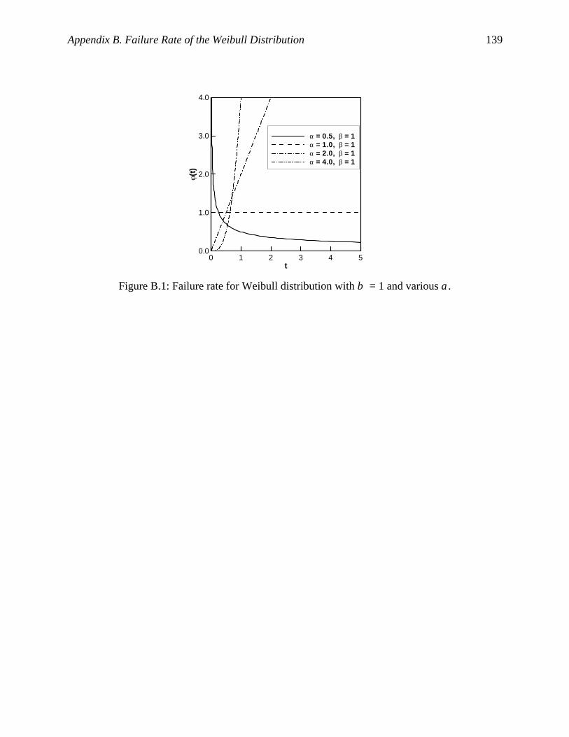
Appendix B. Failure Rate of the Weibull Distribution 139
t
φ(t)
0 1 2 3 4 50.0
1.0
2.0
3.0
4.0
α = 0.5, β = 1α = 1.0, β = 1α = 2.0, β = 1α = 4.0, β = 1
Figure B.1: Failure rate for Weibull distribution with β = 1 and various α.

140
Appendix C Numerical Integration of Joint
Probability Distribution of the Weibull Models
For the indirect approach using differences between two simulation results, the
probability density function (PDF) of the difference is obtained via integration of Eq. 5.12. The
integration has a closed form solution for exponential models. However, for Weibull models,
there is no closed form solution and numerical integration is required. If random variables s and t
are modeled as Weibull,
.exp)(~
exp)(~
2
22
1
11
2
122
1
111
−=
−=
−−
−−
α
αα
α
αα
ββα
ββα
tttht
sssgs
(C.1)
Now, Eq. 5.12 is written as
,0 if exp)( 0 21
112121
21
2121 <
−−
−−∫
∞−−−− xds
xssxss
αα
αααα
ββββαα (C.2)
and
.0 if exp)( x 21
112121
21
2121 >
−−
−−∫
∞−−−− xds
xssxss
αα
αααα
ββββαα (C.3)
Note that the integrand of Eq. C.2 or Eq. C.3 has a singularity at the lower bound of the
integration, when α1 < 1 for Eq. C2 or α2 < 1 for Eq. C3. A technique of change of variable

Appendix C. Numerical Integration of Joint Probability Distribution of the Weibull Models 141
(Ref. [94], p. 163) was utilized to remove the singularities. For Eq. C.2, we change the variable
of integration, s, by introducing ξ such that
.11
1)1(1
1αα ξξ =≡ −+s (C.4)
Now, Eq. C.2 is rewritten as
( ) .0 if exp 0 2
/1
1
1/1212
21
1
2121 <
−−−−∫
∞−−− xd
xx ξ
βξ
βξ
ξββααα
α
αααα (C.5)
Similarly, by introducing
,22
1)1(1
1αα ξξ =≡− −+xs (C.6)
Eq. C3 is rewritten as
( ) .0 if exp 0 21
/11/1
211 2
12
1221 >
−
+−+∫
∞−−− xd
xx ξ
βξ
βξ
ξββα α
αααααα (C.7)
Since the singularities are removed, Eqs. C.5 and C.7 can be numerically integrated. Eqs.
C.5 and C.7 are improper integrals due to the infinite range. In numerical integration, the upper
bound of integration is set to be sufficiently large to guarantee that the contribution of the range
cut off is negligible. Gaussian quadrature of degree of precision three was performed on 100
subintervals logarithmically distributed. The MATLAB source codes for numerical integration
are included in Appendix F.

142
Appendix D Experimental Design of HSCT and
Ws Data
This table contains observation numbers (ID), HSCT configuration design variables (vi)
in a coded form, and Ws data according to convergence settings of GENESIS (see Table 9.1).
ID v1 v2 v3 v4 v5 Ws(A2) Ws(A3) Ws(A5) Ws(B2) Ws(B3) Ws(B5)
1 -1.0000 -1.0000 -1.0000 -1.0000 -1.0000 106332.40 105457.10 105545.20 106094.60 105608.50 105607.50 2 -1.0000 -1.0000 -1.0000 -1.0000 1.0000 167000.50 119731.40 119708.40 130862.10 119878.90 119689.30 3 -1.0000 -1.0000 -1.0000 1.0000 -1.0000 52039.14 51355.46 51194.86 56694.88 51272.82 51244.04 4 -1.0000 -1.0000 -1.0000 1.0000 1.0000 58139.32 57835.40 57739.08 58019.96 57846.68 57796.78 5 -1.0000 -1.0000 1.0000 -1.0000 -1.0000 190725.50 194565.80 191812.00 187808.40 187481.30 182697.10 6 -1.0000 -1.0000 1.0000 -1.0000 1.0000 234341.00 225817.00 220917.00 217070.40 217563.60 215875.20 7 -1.0000 -1.0000 1.0000 1.0000 -1.0000 89058.14 83702.04 83488.70 86268.12 84671.00 83487.62 8 -1.0000 -1.0000 1.0000 1.0000 1.0000 104526.00 96904.66 97306.20 99919.14 99438.82 96857.64 9 -1.0000 1.0000 -1.0000 -1.0000 -1.0000 109287.30 104564.60 104378.00 104537.90 105553.90 104354.80 10 -1.0000 1.0000 -1.0000 -1.0000 1.0000 124378.50 117463.50 117577.90 117568.80 118104.40 117437.50 11 -1.0000 1.0000 -1.0000 1.0000 -1.0000 50933.34 50631.46 50548.68 55400.02 50961.22 50643.84 12 -1.0000 1.0000 -1.0000 1.0000 1.0000 57014.02 57004.92 56915.02 60542.10 56972.50 56956.66 13 -1.0000 1.0000 1.0000 -1.0000 -1.0000 203871.00 200829.80 199567.60 204194.80 202037.20 199517.60 14 -1.0000 1.0000 1.0000 -1.0000 1.0000 263923.40 235927.40 239247.20 237663.40 236686.40 236512.20 15 -1.0000 1.0000 1.0000 1.0000 -1.0000 90722.86 88296.52 87747.98 88677.62 89304.80 87748.90 16 -1.0000 1.0000 1.0000 1.0000 1.0000 102593.50 102595.10 101940.70 113878.40 104394.80 101935.30 17 1.0000 -1.0000 -1.0000 -1.0000 -1.0000 66092.94 65497.42 64124.26 76944.06 70750.98 64139.26 18 1.0000 -1.0000 -1.0000 -1.0000 1.0000 84773.64 69416.90 69334.50 88443.62 69527.42 69560.20 19 1.0000 -1.0000 -1.0000 1.0000 -1.0000 42375.82 42402.96 42374.24 42388.44 42374.74 42374.58 20 1.0000 -1.0000 -1.0000 1.0000 1.0000 45668.54 45442.28 45380.18 45489.02 45386.28 45383.38 21 1.0000 -1.0000 1.0000 -1.0000 -1.0000 101277.90 90567.38 90351.54 91465.70 90695.50 90350.30 22 1.0000 -1.0000 1.0000 -1.0000 1.0000 107276.10 104907.00 104411.00 106736.90 104990.00 104396.60 23 1.0000 -1.0000 1.0000 1.0000 -1.0000 53731.12 51620.70 51606.92 51609.00 51609.52 51606.86 24 1.0000 -1.0000 1.0000 1.0000 1.0000 57268.46 57245.26 57245.22 57747.56 57291.00 57292.04 25 1.0000 1.0000 -1.0000 -1.0000 -1.0000 64612.34 64646.06 64398.98 68080.40 64823.10 64472.42 26 1.0000 1.0000 -1.0000 -1.0000 1.0000 69940.16 69555.72 69643.38 71897.14 69554.16 69556.54 27 1.0000 1.0000 -1.0000 1.0000 -1.0000 42600.66 42660.40 42605.82 43756.36 42600.38 42599.40 28 1.0000 1.0000 -1.0000 1.0000 1.0000 45416.66 45415.04 45414.14 45517.78 45414.72 45414.42 29 1.0000 1.0000 1.0000 -1.0000 -1.0000 92567.38 90904.04 90944.52 93378.46 90906.52 90900.94 30 1.0000 1.0000 1.0000 -1.0000 1.0000 105474.50 105018.40 105026.50 106700.90 106700.70 104996.00 31 1.0000 1.0000 1.0000 1.0000 -1.0000 51865.88 51857.66 51838.60 51839.62 51839.62 51839.34 32 1.0000 1.0000 1.0000 1.0000 1.0000 57868.72 57414.40 57346.32 59077.90 57358.88 57358.88 33 -1.0000 0.0000 0.0000 0.0000 0.0000 100422.00 97777.18 97486.42 102726.90 97947.46 97650.86 34 1.0000 0.0000 0.0000 0.0000 0.0000 58412.00 58954.34 58237.34 58960.66 58627.98 58238.38 35 0.0000 -1.0000 0.0000 0.0000 0.0000 68891.74 67021.44 67182.54 73427.40 67001.24 66999.18 36 0.0000 1.0000 0.0000 0.0000 0.0000 67398.60 66410.72 66321.44 74623.80 67338.62 66394.38 37 0.0000 0.0000 -1.0000 0.0000 0.0000 56398.60 54806.26 54798.16 82663.16 54797.66 54789.08 38 0.0000 0.0000 1.0000 0.0000 0.0000 84875.72 85243.72 84569.36 86252.76 84629.40 84549.32 39 0.0000 0.0000 0.0000 -1.0000 0.0000 104841.30 102452.50 102327.70 116375.90 103165.70 102473.20 40 0.0000 0.0000 0.0000 1.0000 0.0000 53490.94 53236.12 53012.44 59706.26 53137.94 53026.66 41 0.0000 0.0000 0.0000 0.0000 -1.0000 63148.18 62883.12 62889.78 66971.08 62946.30 62932.60 42 0.0000 0.0000 0.0000 0.0000 1.0000 71660.06 71236.48 71281.12 73086.04 71376.78 71242.36 43 0.0000 0.0000 0.0000 0.0000 0.0000 67567.28 67117.62 67008.62 75559.64 67101.84 67087.56 44 -0.7500 -0.7500 -0.7500 -0.7500 -0.7500 93122.32 91426.56 90098.18 90326.06 89649.82 89638.34 45 -0.7500 -0.7500 -0.7500 -0.7500 0.7500 103405.40 99527.36 98378.68 99656.72 98307.74 98261.22 46 -0.7500 -0.7500 -0.7500 0.7500 -0.7500 54127.98 53811.36 53621.48 56364.98 56364.98 53718.84 47 -0.7500 -0.7500 -0.7500 0.7500 0.7500 59951.34 58687.28 58705.32 60451.38 59168.76 58779.54 48 -0.7500 -0.7500 0.7500 -0.7500 -0.7500 152378.30 149592.70 149010.70 151503.80 150682.90 149006.10 49 -0.7500 -0.7500 0.7500 -0.7500 0.7500 175400.80 168567.80 167960.10 170373.30 170373.30 167953.10 50 -0.7500 -0.7500 0.7500 0.7500 -0.7500 86149.28 81560.16 81528.08 83889.06 82245.40 81527.18 51 -0.7500 -0.7500 0.7500 0.7500 0.7500 91730.22 90886.52 90885.88 91762.94 91110.40 90875.34 52 -0.7500 0.7500 -0.7500 -0.7500 -0.7500 89483.68 87773.00 87520.34 88694.28 87622.78 87521.72 53 -0.7500 0.7500 -0.7500 -0.7500 0.7500 96136.06 95762.24 95717.68 105490.30 95715.74 95714.08 54 -0.7500 0.7500 -0.7500 0.7500 -0.7500 52828.56 52662.04 52636.42 58204.50 52739.58 52725.52 55 -0.7500 0.7500 -0.7500 0.7500 0.7500 64513.44 57656.02 57649.02 61382.40 58022.62 57704.88 56 -0.7500 0.7500 0.7500 -0.7500 -0.7500 180922.10 157423.40 156556.00 158775.90 158007.80 156558.60 57 -0.7500 0.7500 0.7500 -0.7500 0.7500 208151.40 177464.30 176256.30 188143.40 178224.70 176258.80 58 -0.7500 0.7500 0.7500 0.7500 -0.7500 85471.04 84258.78 84104.64 87108.06 85489.78 84098.20 59 -0.7500 0.7500 0.7500 0.7500 0.7500 95735.40 94282.86 93990.80 95629.72 94109.74 93986.40

Appendix D. Experimental Design of HSCT and Ws data 143
-----(Continued from the previous page)----- ID v1 v2 v3 v4 v5 Ws(A2) Ws(A3) Ws(A5) Ws(B2) Ws(B3) Ws(B5)
60 0.7500 -0.7500 -0.7500 -0.7500 -0.7500 62413.66 62078.72 61842.98 67439.00 62158.70 61843.70 61 0.7500 -0.7500 -0.7500 -0.7500 0.7500 67047.74 66642.68 66430.50 70209.74 66436.14 66426.16 62 0.7500 -0.7500 -0.7500 0.7500 -0.7500 44480.96 44403.68 44415.34 47057.78 44416.18 44425.62 63 0.7500 -0.7500 -0.7500 0.7500 0.7500 47030.40 46991.16 46975.52 53448.40 46974.30 46975.50 64 0.7500 -0.7500 0.7500 -0.7500 -0.7500 87257.58 85202.66 85240.18 87409.90 85379.06 85199.60 65 0.7500 -0.7500 0.7500 -0.7500 0.7500 98044.42 94847.48 94718.80 95492.50 94678.42 94672.36 66 0.7500 -0.7500 0.7500 0.7500 -0.7500 55973.40 55718.84 55806.66 63814.12 55735.12 55734.90 67 0.7500 -0.7500 0.7500 0.7500 0.7500 63992.06 60334.24 60316.98 61096.46 60326.70 60319.04 68 0.7500 0.7500 -0.7500 -0.7500 -0.7500 61445.64 61396.06 61377.12 73911.84 62919.34 61584.66 69 0.7500 0.7500 -0.7500 -0.7500 0.7500 66449.28 66070.32 66001.70 66068.68 66011.22 66024.14 70 0.7500 0.7500 -0.7500 0.7500 -0.7500 47023.24 44236.30 44239.04 44387.22 44532.00 44524.82 71 0.7500 0.7500 -0.7500 0.7500 0.7500 49123.68 46727.26 46723.76 47105.62 46732.30 46728.84 72 0.7500 0.7500 0.7500 -0.7500 -0.7500 86786.86 86215.90 85996.76 89165.36 85910.22 85913.18 73 0.7500 0.7500 0.7500 -0.7500 0.7500 95913.28 95324.88 95313.70 95837.00 95444.32 95300.98 74 0.7500 0.7500 0.7500 0.7500 -0.7500 56456.18 56010.02 55832.82 55866.54 55836.78 55834.66 75 0.7500 0.7500 0.7500 0.7500 0.7500 60827.32 60442.10 60446.26 60973.76 60475.74 60467.64 76 -0.7500 0.0000 0.0000 0.0000 0.0000 95116.86 88482.68 88496.44 101316.00 88489.30 88485.76 77 0.7500 0.0000 0.0000 0.0000 0.0000 60894.46 59749.10 59712.32 61006.82 59651.90 59649.92 78 0.0000 -0.7500 0.0000 0.0000 0.0000 68762.20 67580.68 67166.50 83693.58 67259.34 67108.56 79 0.0000 0.7500 0.0000 0.0000 0.0000 67001.22 66686.32 66616.24 67430.96 66716.48 66706.32 80 0.0000 0.0000 -0.7500 0.0000 0.0000 57878.92 56412.22 55995.08 70424.04 56188.30 55980.74 81 0.0000 0.0000 0.7500 0.0000 0.0000 84318.34 82705.72 82589.88 84198.34 82884.04 82615.84 82 0.0000 0.0000 0.0000 -0.7500 0.0000 101273.90 90302.30 89994.74 91405.06 90484.88 90035.28 83 0.0000 0.0000 0.0000 0.7500 0.0000 56016.32 55669.00 55641.38 63745.34 55655.14 55654.54 84 0.0000 0.0000 0.0000 0.0000 -0.7500 71287.36 63859.12 63854.64 66971.44 63937.82 63935.66 85 0.0000 0.0000 0.0000 0.0000 0.7500 70524.50 70319.58 70166.34 77578.64 70367.88 70169.70 86 -0.7500 -1.0000 0.2500 0.7500 -1.0000 83912.78 69910.44 69654.36 71329.58 69683.68 69514.26 87 -0.7500 -1.0000 0.7500 -0.2500 -1.0000 127326.70 113382.60 113127.80 116613.50 114088.70 113135.40 88 -0.7500 1.0000 -0.7500 -0.2500 1.0000 79769.12 78895.88 78581.62 86779.58 78673.74 78673.74 89 -0.7500 1.0000 -0.2500 -0.7500 1.0000 134293.90 121008.00 120670.30 134204.90 122791.90 120677.50 90 -0.7500 1.0000 -0.2500 0.7500 1.0000 72148.34 70558.14 69147.70 69543.38 69484.20 69434.86 91 -0.7500 1.0000 0.7500 0.2500 1.0000 113048.50 112831.60 112490.50 114591.00 113543.30 112483.90 92 -0.2500 -1.0000 -0.7500 -0.7500 -1.0000 74372.02 74427.08 74196.26 75564.12 74243.74 74242.86 93 -0.2500 -1.0000 0.7500 0.7500 1.0000 100128.20 75321.84 75007.96 84158.12 75311.36 74991.76 94 -0.2500 1.0000 -0.7500 0.7500 -1.0000 46772.84 46453.24 46439.08 50876.72 46495.58 46480.02 95 0.2500 -1.0000 -0.7500 0.7500 1.0000 51762.92 49085.12 48892.30 54190.26 52377.96 48956.14 96 0.2500 1.0000 -0.7500 -0.7500 1.0000 71309.64 70984.56 70967.40 81046.04 70883.30 70884.74 97 0.2500 1.0000 0.7500 -0.7500 1.0000 114528.00 111356.10 111184.80 146473.30 112490.60 111168.80 98 0.7500 -1.0000 -0.7500 -0.2500 -1.0000 53192.74 53088.46 52775.20 59274.66 53180.18 52853.12 99 0.7500 -1.0000 0.2500 0.7500 -1.0000 51244.04 51262.88 51248.44 51275.88 51253.02 51243.96 100 0.7500 -1.0000 0.7500 -0.2500 1.0000 79352.56 79305.70 79184.68 80004.84 79178.26 79174.36 101 0.7500 1.0000 0.2500 -0.7500 -1.0000 76918.50 77045.24 75830.92 76616.84 76349.94 75828.30 102 0.7500 1.0000 0.7500 0.2500 -1.0000 61628.70 61363.60 61358.84 61376.60 61396.96 61350.48 103 -0.7500 -1.0000 -0.7500 0.2500 -1.0000 60927.40 60408.52 60352.74 63110.08 60563.26 60383.58 104 -0.2500 -1.0000 0.7500 -0.7500 1.0000 152999.00 134714.00 134651.30 139712.70 135717.50 134642.20 105 -0.2500 1.0000 -0.7500 -0.7500 -1.0000 72682.30 72190.86 72190.92 73671.94 72209.22 72196.98 106 -0.2500 1.0000 0.7500 -0.7500 -1.0000 119817.70 118773.40 118819.70 124480.20 118770.40 118769.70 107 -0.2500 1.0000 0.7500 0.7500 -1.0000 67422.86 67370.88 67029.92 67172.94 67164.80 67035.38 108 0.2500 -1.0000 -0.7500 -0.7500 1.0000 81461.52 72636.32 72504.52 85316.16 72880.92 72513.34 109 0.2500 -1.0000 0.7500 -0.7500 -1.0000 96498.06 95697.48 95243.94 96193.96 95356.12 95399.74 110 0.2500 1.0000 -0.7500 0.7500 -1.0000 44829.96 44345.86 44310.30 47788.98 44319.92 44311.96 111 0.2500 1.0000 0.7500 0.7500 1.0000 66612.16 66337.86 66322.34 66839.98 66318.64 66317.82 112 0.7500 1.0000 -0.7500 0.2500 1.0000 52368.60 51507.82 51464.46 55315.24 57378.02 51489.00 113 -1.0000 -0.3333 -0.3333 -0.3333 -0.3333 95690.64 95190.58 94566.34 97228.48 96506.76 94541.92 114 -1.0000 0.3333 0.3333 0.3333 0.3333 112135.90 103692.40 101670.90 135873.20 103035.90 101670.30 115 -0.3333 -1.0000 -0.3333 0.3333 1.0000 67204.94 64545.60 64337.98 69251.90 64847.40 64385.22 116 -0.3333 -0.3333 -1.0000 1.0000 0.3333 47391.50 47408.80 47323.92 49485.54 47354.52 47362.22 117 -0.3333 0.3333 1.0000 -1.0000 -0.3333 155274.80 151927.90 149467.40 158219.90 150680.00 149447.40 118 -0.3333 1.0000 0.3333 -0.3333 -1.0000 91446.70 89071.58 88563.30 90144.84 88873.14 88624.58 119 0.3333 -1.0000 0.3333 1.0000 -0.3333 53456.92 53397.88 53382.92 54215.84 54215.84 53387.88 120 0.3333 -0.3333 1.0000 0.3333 -1.0000 65997.12 65666.22 65641.32 66512.42 65883.84 65622.96 121 0.3333 0.3333 -1.0000 -0.3333 1.0000 60000.64 60147.52 59978.32 66422.10 59991.08 60001.44 122 0.3333 1.0000 -0.3333 -1.0000 0.3333 97324.00 83220.44 82868.60 87033.42 83250.00 82814.44 123 1.0000 -1.0000 1.0000 -0.3333 0.3333 82599.14 76292.38 76196.84 76983.96 76196.46 76194.60 124 1.0000 -0.3333 0.3333 -1.0000 1.0000 93147.72 93717.76 92378.96 92596.24 92647.28 92349.98 125 1.0000 0.3333 -0.3333 1.0000 -1.0000 44493.46 44494.92 44491.44 44535.08 44491.70 44491.62 126 1.0000 1.0000 -1.0000 0.3333 -0.3333 49267.06 47533.12 47641.70 51293.52 47555.22 47542.42

144
Appendix E MATLAB Code for Direct Fit of
Weibull Model to Optimization Errors
This MATLAB source code is used to fit the Weibull model to the error of Case A2. It
reads in data files of optimal wing structural weight (Ws). It calculates the error with respect to
the best of the six runs from different GENESIS parameter settings. As an output, a QQ plot is
generated. It also prints out histograms and cumulative frequencies to compare data and fit. The
results of χ2 goodness-of-fit test are printed.
clear all; %%%%%%%%%%%%%%%%%%%%%%%%%%%%%%%%%%%%%% % read in Ws data stored in files %%%%%%%%%%%%%%%%%%%%%%%%%%%%%%%%%%%%%% %Case A2 fid=fopen('Ws.CaseA2.dat','r'); WsA2=fscanf(fid,'%g'); fclose(fid); %Case A3 fid=fopen('Ws.CaseA3.dat','r'); WsA3=fscanf(fid,'%g'); fclose(fid); %Case A5 fid=fopen('Ws.CaseA5.dat','r'); WsA5=fscanf(fid,'%g'); fclose(fid); %Case B2 fid=fopen('Ws.CaseB2.dat','r'); WsB2=fscanf(fid,'%g'); fclose(fid); %Case B3 fid=fopen('Ws.CaseB3.dat','r'); WsB3=fscanf(fid,'%g'); fclose(fid); %Case B5 fid=fopen('Ws.CaseB5.dat','r'); WsB5=fscanf(fid,'%g'); fclose(fid); % observation index index=[1:length(WsA2)]'; %%%%%%%%%%%%%%%%%%%%%%%%%%%%%%%%%%%%%%%%%%%%%%%%%%% % estimate true Ws by taking the best of six cases %%%%%%%%%%%%%%%%%%%%%%%%%%%%%%%%%%%%%%%%%%%%%%%%%%% Wst=(min([WsA2 WsA3 WsA5 WsB2 WsB3 WsB5]'))'; % calculate error of Case A2 X=(WsA2-Wst); % sort the error data X=sort(X); % Find id numbers of data points of nonzero values non0X=find(X);

Appendix E. MATLAB Code for Direct Fit of Weibull Model to Optimization Errors 145
% add offset to avoid singularity of X=0 for alpha < 1 if length(non0X) == length(X) os=0.; else os=min( .00001*mean(X), X(non0X(1)) ); end X=X+os; %%%%%%%%%%%%%%%%%%%%%%%%%%%%%%%%%%%%%%%%%%%%%%%%%%%%%%%%%%%%%% % Fitting Weibull model to the data % % weibfit from MATLAB statistics toolbox % Use 5% confidence level % Estimated parameters are returned to mu % Confidence interval of mu are returned to muci %%%%%%%%%%%%%%%%%%%%%%%%%%%%%%%%%%%%%%%%%%%%%%%%%%%%%%%%%%%%%% [mu muci]=weibfit(X,.05) mu1=mu(1); mu2=mu(2); % MATLAB uses parameters in a different form. Convert them to alpha and beta. alpha=mu(2); beta=(1/mu1)^(1/mu2); % Calculate Log likelihood function for the estimated parameters ONES=ones(length(X),1); LL=sum( log( weibpdf(X,mu1*ONES,mu2*ONES) ) ) %%%%%%%%%%%%%%%%%%%%%%%%%%%%%%%%%%%%%%%%%%%%%%%%%%%% % Generating QQ plot between data and fit % % invX: expected location of X from fit %%%%%%%%%%%%%%%%%%%%%%%%%%%%%%%%%%%%%%%%%%%%%%%%%%%% pX=( ([1:length(X)]-.5)./length(X) )'; invX=weibinv(pX,mu1,mu2); maxX=max([max(invX) max(X)]); XSCL=[1 10 100 1000 10000 100000]; ISCL=find( maxX./XSCL < 10 ); SCL=XSCL(ISCL(1)); xrange=SCL*round(max([max(invX) max(X)])/SCL+.5); figure; plot(invX,X,'r+',[0 xrange],[0 xrange],'b-'); % axis equal axis([0 xrange 0 xrange]); set(gca,'xtick',[0:SCL:xrange]); set(gca,'ytick',[0:SCL:xrange]); set(gca,'XTickLabel',[0:SCL:xrange]); set(gca,'YTickLabel',[0:SCL:xrange]); set(gca,'FontSize',15); xlabel('X Quantiles(Fit)','FontSize',15); ylabel('Y Quantiles(Data)','FontSize',15); fid=fopen('qqWEIBcaseA2.plt','w'); fprintf(fid,'%15.7e %15.7e %15.7e\n',… [invX X (linspace(0,xrange,length(X)))' ]'); fclose(fid); %%%%%%%%%%%%%%%%%%%%%%%%%%%%%%%%%%%%%%%%%%%%%%%%%%%%%%%%%%%%%%%%%%%%%%% % GENERATE data for histogram and cumulative frequency plot % % BND : subintervals % XBND: center point of subintervals % IBIN: frequencies of data % SBIN: Cumulative frequencies of data % RBIN: complementary cumulative frequencies, (Total # of data)-SBIN % XFRQexp: expected frequencies from the fit

Appendix E. MATLAB Code for Direct Fit of Weibull Model to Optimization Errors 146
% CFRQexp: expected cumulative frequencies from the fit %%%%%%%%%%%%%%%%%%%%%%%%%%%%%%%%%%%%%%%%%%%%%%%%%%%%%%%%%%%%%%%%%%%%%%%% nbin=50; MpctL=0; %MpctU=xrange; MpctU=SCL*round(max(X)/SCL+.5); Mpct=MpctU-MpctL; binsize=Mpct/nbin; BND=[MpctL :binsize:MpctU]'; for n=1:nbin XBND(n,1)=.5*( BND(n)+BND(n+1) ); end % IBIN=zeros([nbin 1]); SBIN=zeros([nbin 1]); RBIN=zeros([nbin 1]); for k=1:length(X) ibin=floor( (X(k)-MpctL)/binsize ) + 1 ; IBIN(ibin)=IBIN(ibin)+1; end % SBIN(1)=IBIN(1); for n=2:nbin SBIN(n)=SBIN(n-1)+IBIN(n); end % for n=1:nbin RBIN(n)=length(X)-SBIN(n); end % for i=1:nbin Xexp(i,1)=weibcdf(BND(i+1),mu1,mu2)-weibcdf(BND(i),mu1,mu2); XFRQexp(i,1)=length(X)*Xexp(i); CFRQexp(i,1)=length(X)*weibcdf(BND(i+1),mu1,mu2); end % print out histogram data as TECPLOT format fid=fopen('WEIBcaseA2hist.plt','w'); fprintf(fid,'variables=XBND,IBIN,XFRQexp\n'); fprintf(fid,'%13.5e %13.5e %13.5e \n',[XBND IBIN XFRQexp ]'); fclose(fid); % print out CDF data as TECPLOT format fid=fopen('WEIBcaseA2cdf.plt','w'); fprintf(fid,'variables=BND,SBIN,CFRQexp\n'); fprintf(fid,'%13.5e %13.5e %13.5e \n',[BND(2:end) SBIN CFRQexp ]'); fclose(fid); %return to original data X=X-os; %%%%%%%%%%%%%%%%%%%%%%%%%%%%%%%%%%%%%%%%%%%%%%%%%%%% % Chi-square goodness of fit TEST % % nb: # of intervals for Chi-square test % ip: x-locations of the intervals having the same probability % IX: prob( x < x_i), probability that x is less than the i-th observation % IB: number of data points belong to each interval %%%%%%%%%%%%%%%%%%%%%%%%%%%%%%%%%%%%%%%%%%%%%%%%%%%% nb=10; nbi=1./nb; p=[0 : nbi : 1] np=length(X)*nbi; for i=1:length(p)-1 ip(i,1)=weibinv(p(i),mu1,mu2); end

Appendix E. MATLAB Code for Direct Fit of Weibull Model to Optimization Errors 147
ip(length(p),1)=Inf; % for i=1:length(X) IX(i)=weibcdf(X(i),mu1,mu2); end IB=zeros([nb 1]); for k=1:length(X) if IX(k) == 0 IB(1)=IB(1)+1; elseif IX(k) ==1 IB(end)=IB(end)+1; else ib=floor( (IX(k)-p(1))/nbi ) + 1 ; IB(ib)=IB(ib)+1; end end sum(IB) % fprintf('%3d %12.5e %12.5e %3d %12.5e %12.5e %12.5e\n', ... [ [1:nb]' ip(1:end-1) ip(2:end) IB np*ones(nb,1) (IB-np) (IB-np).^2/np]'); X2=sum( (IB-np).^2 )/np; %chi2cdf(X2,nb-1) pvalue=1-chi2cdf(X2,nb-1-2); fprintf('%15.4f %15.4f\n',[mu1 mu2]); meanE=beta/alpha*gamma(1/alpha); varE=beta^2/alpha*( 2*gamma(2/alpha)-1/alpha*(gamma(1/alpha))^2 ); stdE=sqrt(varE); fprintf(' alpha=%15.4f\n beta=%15.4f\n meanE=%15.4f\n stdE=%15.4f\n',... [alpha beta meanE stdE]); fprintf(' X^2=%15.4f\n pvalue=%15.4f\n',[X2 pvalue]);

148
Appendix F MATLB Code for Indirect Fit of
Weibull Model to Optimization Errors
INDIRECTFIT.m reads in Ws data files and performs the indirect fit of differences
between Cases A2 and A3. A set of distribution parameters are sought to maximize the log
likelihood function by using a constrained minimization routine, fmincon, from the optimization
toolbox of MATLAB [86]. LOGL.m calculates the negative of the log likelihood function.
WJIM.m and WJIP.m are integrands of convolution for x < 0 and x > 0, respectively (see Eqs.
C.5 and C.7 in Appendix C). COSLOGSPACE.m is used to generate intervals for numerical
integration. The outputs are the parameters of the Weibull models for Cases A2 and A3 and the
χ2 test results for the fit on the differences.
INDIRECTFIT.m clear all; %%%%%%%%%%%%%%%%%%%%%%%%%%%%%%%%%%%%%% % read in Ws data stored in files %%%%%%%%%%%%%%%%%%%%%%%%%%%%%%%%%%%%%% %Case A2 fid=fopen('Ws.CaseA2.dat','r'); WsA2=fscanf(fid,'%g'); fclose(fid); %Case A3 fid=fopen('Ws.CaseA3.dat','r'); WsA3=fscanf(fid,'%g'); fclose(fid); %Case A5 fid=fopen('Ws.CaseA5.dat','r'); WsA5=fscanf(fid,'%g'); fclose(fid); %Case B2 fid=fopen('Ws.CaseB2.dat','r'); WsB2=fscanf(fid,'%g'); fclose(fid); %Case B3 fid=fopen('Ws.CaseB3.dat','r'); WsB3=fscanf(fid,'%g'); fclose(fid); %Case B5 fid=fopen('Ws.CaseB5.dat','r'); WsB5=fscanf(fid,'%g'); fclose(fid); % observation index index=[1:length(WsA2)]'; %%%%%% calculate differences between Case A2 and Case A3 X=(WsA2-WsA3);

Appendix F. MATLAB Code for Indirect Fit of Weibull Model to Optimization Errors 149
% perturb data of x = 0 npt=length(X); izero=find(X==0); if length(izero) > 0 X(izero)=0.5*( X(izero(1)-1) +X(izero(end)+1) ); end %%%%%%%%%%%%%%%%%%%%%%%%%%%%%%%%%%%%%%%%%%%%%%%%%%%%%%%%%%%%%%%%%%%%%%%%% % Minimization of LOGL.m % using fmincon of optimization toolbox of MATLAB % LOGL.m : objective function, calculate -loglikelihood % beta's are scaled (multiplied by 0.001 ) to prevent % numerical difficulties during optimization %%%%%%%%%%%%%%%%%%%%%%%%%%%%%%%%%%%%%%%%%%%%%%%%%%%%%%%%%%%%%%%%%%%%%%%%% OPTIONS=optimset('Diagnostics',1,'Display','iter','MaxIter',30,'MaxFunEvals',1000); [B,FVAL,EXITFLAG]= fmincon('LOGL',[0.7663 3.9012907 0.4703 0.3058443],... [],[],[],[],[.3 2 .1 0.01],[.8 8 .6 1.],[],OPTIONS,X); % Rescale beta's B(2)=1000*B(2); B(4)=1000*B(4); %%%%%%%%%%%%%%%%%%%%%%%%%%%%%%%%%%%%%%%%%%%%%%%%%%% % Generate empirical CDF of differences % mc: size of sample % R1: weibull random numbers for Case A2 % R2: weibull random numbers for Case A3 % RDIFF: R1-R2, sorted %%%%%%%%%%%%%%%%%%%%%%%%%%%%%%%%%%%%%%%%%%%%%%%%%%% mc=100; rand('state',0); % R1=weibrnd(B(2)^(-(B(1))),B(1),npt*mc,1); R2=weibrnd(B(4)^(-(B(3))),B(3),npt*mc,1); RDIFF=sort(R1-R2); %%%%%%%%%%%%%%%%%%%%%%%%%%%%%%%%%%%%%%%%%%%%%%%%%%%% % Chi-square goodness of fit TEST for the difference fit % % nb: # of intervals for Chi-square test % ip: x-locations of the intervals having the same probability % IB: number of data points belong to each interval %%%%%%%%%%%%%%%%%%%%%%%%%%%%%%%%%%%%%%%%%%%%%%%%%%%% nb=10; nbi=1./nb; p=[0 : nbi : 1]; np=length(X)*nbi; ip(1,1)=RDIFF(1); for i=2:length(p)-1 ip(i,1)=RDIFF( round( (length(RDIFF)*p(i)) ) ); end ip(length(p),1)=RDIFF(end); % IB=zeros([nb 1]); for i=1:length(X) if X(i) < ip(2) IB(1)=IB(1)+1; elseif X(i) >= ip(end-1) IB(end)=IB(end)+1; else j=2; while ~( ip(j) <= X(i) & ip(j+1) > X(i) ) j=j+1; end IB(j)=IB(j)+1;

Appendix F. MATLAB Code for Indirect Fit of Weibull Model to Optimization Errors 150
end end sum(IB) % fprintf('%3d %12.5e %12.5e %3d %12.5e %12.5e %12.5e\n', ... [ [1:nb]' ip(1:end-1) ip(2:end) IB np*ones(nb,1) (IB-np) (IB-np).^2/np]'); X2=sum( (IB-np).^2 )/np %chi2cdf(X2,nb-1); pvalue=1.-chi2cdf(X2,nb-4-1); alpha1=B(1); beta1=B(2); alpha2=B(3); beta2=B(4); fprintf(' alpha1=%12.5e\n beta1=%12.5e\n alpha2=%12.5e\n beta2=%12.5e\n',... alpha1,beta1,alpha2,beta2); fprintf(' X^2=%12.5e\n pvalue=%12.5e\n',X2,pvalue); LOGL.m function R=LOGL(B,XS); npt=length(XS); id=[]; % return to original scale B(2)=1000.*B(2); B(4)=1000.*B(4); % large enough upper bound of integration Irange=100000; % fprintf(1,'B = %15.7e %15.7e %15.7e %15.7e\n',B); for i=1:npt if XS(i) < 0 s_0=0; s_1=s_0+Irange; s_0=s_0^B(1); s_1=s_1^B(1); elseif XS(i) > 0 s_0=XS(i); s_1=s_0+Irange; s_0=(s_0-XS(i))^B(3); s_1=(s_1-XS(i))^B(3); else fprintf('x is zero, perturb it \n'); end %%%%%%%%%%%%%%%%%%%%%%%%%%%%%%%%%%%%%%%%%%%%%%%%%%%%%%%%%%%%%%%%%%% % set subintervals for integration % - use logarithmic distribution to use dense intervals near lower bound % - use offset to prevent too dense s near zero %%%%%%%%%%%%%%%%%%%%%%%%%%%%%%%%%%%%%%%%%%%%%%%%%%%%%%%%%%%%%%%%%%%% offset=0.1*s_1; s=COSLOGSPACE(log10(s_0+offset),log10(s_1+offset),101); s=s-offset; s(1)=s_0; % Gaussian quadrature of third order accuracy n=length(s)-1; for j=1:n a=s(j); b=s(j+1); c1=1; c2=1;

Appendix F. MATLAB Code for Indirect Fit of Weibull Model to Optimization Errors 151
t1=-1/sqrt(3); t2= 1/sqrt(3); s1=.5*((b-a)*t1+a+b); s2=.5*((b-a)*t2+a+b); % WJIM: integrand for x < 0 % WJIP: integrand for x > 0 if XS(i) < 0 fsum(j)=.5*(b-a)* (c1*WJIM(s1,XS(i),B)+c2*WJIM(s2,XS(i),B)); else fsum(j)=.5*(b-a)* (c1*WJIP(s1,XS(i),B)+c2*WJIP(s2,XS(i),B)); end end f(i)=sum(fsum); end % negative of loglikelihood for minimization R=-sum( log(f) ); fprintf(1,'OBJ = %15.7e\n',R); WJIM.m function f=WJIM(s,x,B); % integrand for x < 0 a1=B(1); b1=B(2); a2=B(3); b2=B(4); % f=a2*b1^(-a1)*b2^(-a2)*(s.^(1/a1)-x).^(a2-1).*exp(-s./(b1.^a1)-((s.^(1/a1)-x)./b2).^a2); WJIP.m function f=WJIP(s,x,B); % integrand for x > 0 a1=B(1); b1=B(2); a2=B(3); b2=B(4); % f=a1*b1^(-a1)*b2^(-a2)*(s.^(1/a2)+x).^(a1-1).*exp(-s./(b2.^a2)-((s.^(1/a2)+x)./b1).^a1); COSLOGSPACE.m function y = COSLOGSPACE(d1, d2, n) % generate highly stretched intervals between d1 and d2 by % combining cosine and log pw=d1+(d2-d1)*(1-cos(linspace(0,.5*pi,n))).^2; y=10.^pw;
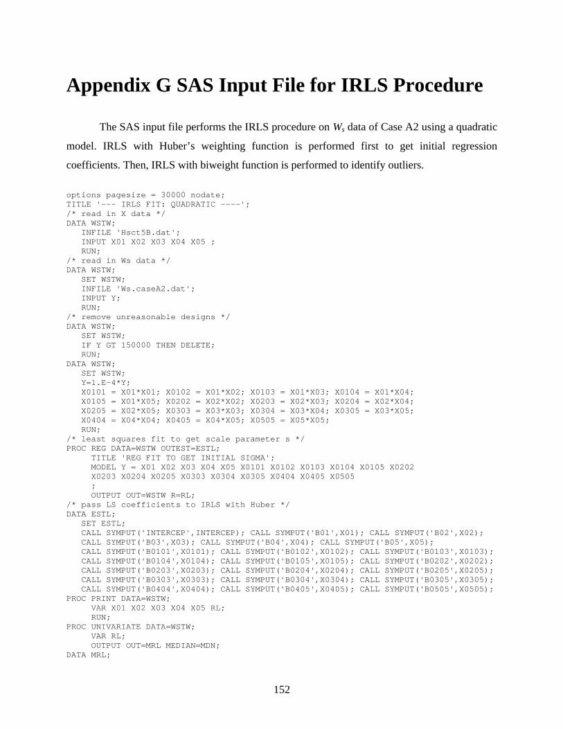
152
Appendix G SAS Input File for IRLS Procedure
The SAS input file performs the IRLS procedure on Ws data of Case A2 using a quadratic
model. IRLS with Huber’s weighting function is performed first to get initial regression
coefficients. Then, IRLS with biweight function is performed to identify outliers.
options pagesize = 30000 nodate; TITLE '--- IRLS FIT: QUADRATIC ----'; /* read in X data */ DATA WSTW; INFILE 'Hsct5B.dat'; INPUT X01 X02 X03 X04 X05 ; RUN; /* read in Ws data */ DATA WSTW; SET WSTW; INFILE 'Ws.caseA2.dat'; INPUT Y; RUN; /* remove unreasonable designs */ DATA WSTW; SET WSTW; IF Y GT 150000 THEN DELETE; RUN; DATA WSTW; SET WSTW; Y=1.E-4*Y; X0101 = X01*X01; X0102 = X01*X02; X0103 = X01*X03; X0104 = X01*X04; X0105 = X01*X05; X0202 = X02*X02; X0203 = X02*X03; X0204 = X02*X04; X0205 = X02*X05; X0303 = X03*X03; X0304 = X03*X04; X0305 = X03*X05; X0404 = X04*X04; X0405 = X04*X05; X0505 = X05*X05; RUN; /* least squares fit to get scale parameter s */ PROC REG DATA=WSTW OUTEST=ESTL; TITLE 'REG FIT TO GET INITIAL SIGMA'; MODEL Y = X01 X02 X03 X04 X05 X0101 X0102 X0103 X0104 X0105 X0202 X0203 X0204 X0205 X0303 X0304 X0305 X0404 X0405 X0505 ; OUTPUT OUT=WSTW R=RL; /* pass LS coefficients to IRLS with Huber */ DATA ESTL; SET ESTL; CALL SYMPUT('INTERCEP',INTERCEP); CALL SYMPUT('B01',X01); CALL SYMPUT('B02',X02); CALL SYMPUT('B03',X03); CALL SYMPUT('B04',X04); CALL SYMPUT('B05',X05); CALL SYMPUT('B0101',X0101); CALL SYMPUT('B0102',X0102); CALL SYMPUT('B0103',X0103); CALL SYMPUT('B0104',X0104); CALL SYMPUT('B0105',X0105); CALL SYMPUT('B0202',X0202); CALL SYMPUT('B0203',X0203); CALL SYMPUT('B0204',X0204); CALL SYMPUT('B0205',X0205); CALL SYMPUT('B0303',X0303); CALL SYMPUT('B0304',X0304); CALL SYMPUT('B0305',X0305); CALL SYMPUT('B0404',X0404); CALL SYMPUT('B0405',X0405); CALL SYMPUT('B0505',X0505); PROC PRINT DATA=WSTW; VAR X01 X02 X03 X04 X05 RL; RUN; PROC UNIVARIATE DATA=WSTW; VAR RL; OUTPUT OUT=MRL MEDIAN=MDN; DATA MRL;

Appendix G. SAS Input File for IRLS Procedure 153
SET MRL; CALL SYMPUT('MDN',MDN); DATA WSTW; SET WSTW; MAD=ABS(RL-&MDN); PROC UNIVARIATE DATA=WSTW; VAR MAD; OUTPUT OUT=MADSET MEDIAN=MMAD; DATA MADSET; SET MADSET; CALL SYMPUT('MMAD',MMAD); /* IRLS fit with Huber weighting function to get initial coeff */ PROC NLIN DATA=WSTW NOHALVE MAXITER=1000 OUTEST=ESTP; TITLE 'NONLINEAR REGRESSION TO GET IRLS INITIAL COEFF'; PARMS INTERCEP = &INTERCEP B01 = &B01 B02 = &B02 B03 = &B03 B04 = &B04 B05 = &B05 B0101 = &B0101 B0102 = &B0102 B0103 = &B0103 B0104 = &B0104 B0105 = &B0105 B0202 = &B0202 B0203 = &B0203 B0204 = &B0204 B0205 = &B0205 B0303 = &B0303 B0304 = &B0304 B0305 = &B0305 B0404 = &B0404 B0405 = &B0405 B0505 = &B0505 ; MODEL Y = INTERCEP +B01*X01 +B02*X02 +B03*X03 +B04*X04 +B05*X05 +B0101*X0101 +B0102*X0102 +B0103*X0103 +B0104*X0104 +B0105*X0105 +B0202*X0202 +B0203*X0203 +B0204*X0204 +B0205*X0205 +B0303*X0303 +B0304*X0304 +B0305*X0305 +B0404*X0404 +B0405*X0405 +B0505*X0505 ; DER.INTERCEP = 1; DER.B01=X01; DER.B02=X02; DER.B03=X03; DER.B04=X04; DER.B05=X05; DER.B0101=X0101; DER.B0102=X0102; DER.B0103=X0103; DER.B0104=X0104; DER.B0105=X0105; DER.B0202=X0202; DER.B0203=X0203; DER.B0204=X0204; DER.B0205=X0205; DER.B0303=X0303; DER.B0304=X0304; DER.B0305=X0305; DER.B0404=X0404; DER.B0405=X0405; DER.B0505=X0505; R=Y-MODEL.Y; SIG=1.4826*&MMAD; H=1.; RPS=ABS(R/SIG); IF RPS <= H THEN _WEIGHT_=1.; ELSE _WEIGHT_= H/RPS; OUTPUT OUT=WSTW R=RP; DATA WSTW; SET WSTW; SIG=1.4826*&MMAD; H=1.0; RPS=ABS(RP/SIG);

Appendix G. SAS Input File for IRLS Procedure 154
IF RPS <= H THEN _WEIGHT_=1.; ELSE _WEIGHT_= H/RPS; PROC PRINT DATA=WSTW; VAR X01 X02 X03 X04 X05 SIG RL RP RPS H _WEIGHT_; RUN; PROC UNIVARIATE DATA=WSTW; VAR RP; OUTPUT OUT=MRP MEDIAN=MDN2; DATA MRP; SET MRP; CALL SYMPUT('MDN2',MDN2); DATA WSTW; SET WSTW; MAD2=ABS(RP-&MDN2); PROC UNIVARIATE DATA=WSTW; VAR MAD2; OUTPUT OUT=MADSET2 MEDIAN=MMAD2; DATA MADSET2; SET MADSET2; CALL SYMPUT('MMAD2',MMAD2); PROC PRINT DATA=ESTP; RUN; DATA ESTP; SET ESTP; IF _TYPE_ ~= 'FINAL' THEN DELETE; PROC PRINT DATA=ESTP; RUN; /* pass coefficients to IRLS with biweight */ DATA ESTP; SET ESTP; CALL SYMPUT('INTERCEP',INTERCEP); CALL SYMPUT('B01',B01); CALL SYMPUT('B02',B02); CALL SYMPUT('B03',B03); CALL SYMPUT('B04',B04); CALL SYMPUT('B05',B05); CALL SYMPUT('B0101',B0101); CALL SYMPUT('B0102',B0102); CALL SYMPUT('B0103',B0103); CALL SYMPUT('B0104',B0104); CALL SYMPUT('B0105',B0105); CALL SYMPUT('B0202',B0202); CALL SYMPUT('B0203',B0203); CALL SYMPUT('B0204',B0204); CALL SYMPUT('B0205',B0205); CALL SYMPUT('B0303',B0303); CALL SYMPUT('B0304',B0304); CALL SYMPUT('B0305',B0305); CALL SYMPUT('B0404',B0404); CALL SYMPUT('B0405',B0405); CALL SYMPUT('B0505',B0505); /* IRLS with biweight */ PROC NLIN DATA=WSTW NOHALVE MAXITER=1000 ; TITLE 'NONLINEAR REGRESSION TO GET IRLS FIT'; PARMS INTERCEP = &INTERCEP B01 = &B01 B02 = &B02 B03 = &B03 B04 = &B04 B05 = &B05 B0101 = &B0101 B0102 = &B0102 B0103 = &B0103 B0104 = &B0104 B0105 = &B0105 B0202 = &B0202 B0203 = &B0203 B0204 = &B0204 B0205 = &B0205 B0303 = &B0303 B0304 = &B0304 B0305 = &B0305 B0404 = &B0404

Appendix G. SAS Input File for IRLS Procedure 155
B0405 = &B0405 B0505 = &B0505 ; MODEL Y = INTERCEP +B01*X01 +B02*X02 +B03*X03 +B04*X04 +B05*X05 +B0101*X0101 +B0102*X0102 +B0103*X0103 +B0104*X0104 +B0105*X0105 +B0202*X0202 +B0203*X0203 +B0204*X0204 +B0205*X0205 +B0303*X0303 +B0304*X0304 +B0305*X0305 +B0404*X0404 +B0405*X0405 +B0505*X0505 ; DER.INTERCEP=1; DER.B01=X01; DER.B02=X02; DER.B03=X03; DER.B04=X04; DER.B05=X05; DER.B0101=X0101; DER.B0102=X0102; DER.B0103=X0103; DER.B0104=X0104; DER.B0105=X0105; DER.B0202=X0202; DER.B0203=X0203; DER.B0204=X0204; DER.B0205=X0205; DER.B0303=X0303; DER.B0304=X0304; DER.B0305=X0305; DER.B0404=X0404; DER.B0405=X0405; DER.B0505=X0505; R=Y-MODEL.Y; B=1.9; SIG2=1.4826*&MMAD2; RBS=ABS(R/SIG2); IF RBS <= B THEN _WEIGHT_=(1.-(RBS/B)**2)**2; ELSE _WEIGHT_=0.; OUTPUT OUT=WSTW R=RB; RUN; DATA WSTW; SET WSTW; B=1.9; SIG2=1.4826*&MMAD2; RBS=ABS(RB/SIG2); IF RBS <= B THEN _WEIGHT_=(1.-(RBS/B)**2)**2; ELSE _WEIGHT_=0.; /* print out results */ PROC PRINT DATA=WSTW; VAR X01 X02 X03 X04 X05 SIG SIG2 RL RP RPS RB RBS B _WEIGHT_; RUN;

156
VITA Hongman Kim was born on July 31, 1970 in Pusan, South Korea. In 1993, He graduated with his
B.S. degree in Aerospace Engineering from Seoul National University in South Korea. After he
earned his M.S. degree in Aerospace Engineering in 1995 from the same school, he worked as a
staff scientist in the application of computational fluid dynamics at Systems Engineering
Research Institute in Taejon, South Korea. In August 1997, he continued his study at Virginia
Tech and earned his Ph.D. degree in Aerospace Engineering in June 2001. While working as a
graduate research assistant at Virginia Tech, he joined a team of faculty and graduate students
working on advanced techniques in multidisciplinary design and optimization of a high-speed
civil transport.