HAL Id: tel-00798576https://tel.archives-ouvertes.fr/tel-00798576

Submitted on 8 Mar 2013

HAL is a multi-disciplinary open accessarchive for the deposit and dissemination of sci-entific research documents, whether they are pub-lished or not. The documents may come fromteaching and research institutions in France orabroad, or from public or private research centers.

L’archive ouverte pluridisciplinaire HAL, estdestinée au dépôt et à la diffusion de documentsscientifiques de niveau recherche, publiés ou non,émanant des établissements d’enseignement et derecherche français ou étrangers, des laboratoirespublics ou privés.

Statistical Post-Processing Methods And TheirImplementation On The Ensemble Prediction Systems

For Forecasting Temperature In The Use Of The FrenchElectric Consumption

Adriana Geanina Gogonel

To cite this version:Adriana Geanina Gogonel. Statistical Post-Processing Methods And Their Implementation On TheEnsemble Prediction Systems For Forecasting Temperature In The Use Of The French Electric Con-sumption. General Mathematics [math.GM]. Université René Descartes - Paris V, 2012. English.�NNT : 2012PA05S014�. �tel-00798576�

Université Paris DescartesLaboratoire MAP 5

École Doctorale de Sciences Mathématiques de Paris Centre

THÈSEpour obtenir le grade de

Docteur en Mathématiques Appliquéesde l’Université Paris Descartes

Spécialité : STATISTIQUE

Présentée par Adriana CUCU GOGONEL

Statistical Post-Processing Methods And Their Implementation On The EnsemblePrediction Systems For Forecasting Temperature In The Use Of The French Electric

Consumption.

Thèse dirigée parAvner BAR-HEN

soutenue publiquement le 27 novembre 2012

Jury

Rapporteurs Jerome Saracco, Institut Polytechnique de BordeauxJocelyn Gaudet, Hydro-Québec

Examinatrice Virginie Dordonnat, EDF R&DExaminateur Eric Parent, AgroParisTech/INRADirecteurs de thèse Avner Bar-Hen, Université Paris Descartes

Jérôme Collet, EDF R&D

Remerciements

Je voudrais en premier lieu remercier les personnes qui ont rendu possible l’existence decette thèse, je pense à mon directeur de thèse, Avner Bar-Hen et à mon encadrant EDF,Jérôme Collet. Je remercie Avner d’avoir bien voulu assumer la direction de cette thèse.Son soutien, sa bonne humeur, sa disponibilité et son exigence ont été des éléments indis-pensables à la réussite de ce travail. Je remercie Jérôme qui m’a fait découvrir la rechercheet m’a donné le gout du SAS. Il a toujours su se rendre disponible et me faire bénéficierde son expérience tout en me laissant une grande liberté d’action.

Je tiens à exprimer ma gratitude aux personnes qui m’ont fait l’honneur de participerau jury de cette thèse. Je suis reconnaissante envers Jérôme Saracco et Jocelyn Gaudetpour l’intérêt qu’ils ont porté à cette thèse en acceptant d’en être les rapporteurs, leursrapports m’ont permis d’améliorer ce manuscrit. Je suis particulièrement reconnaissante àVirginie Dordonnat, pour ses conseils précieux dans tous les domaines : technique, métier,valorisation du travail, écriture du rapport ainsi que pour son soutien continu qui a étéd’autant plus précieux dans mes moments de doutes. Je tiens à remercier également EricParent de m’avoir fait part de ses idées sur mes travaux, ce qui m’a ouvert des perspectivespour la suite de la thèse.

Je remercie mes collègues Julien Najac, Laurent Dubus, Thi-Thu Huong-Hoang, ChristopheChaussin et Marc Voirin d’avoir participé aux réunions de suivi de ma thèse. Ces réunionsont toujours été d’une aide importante dans l’évolution des travaux de thèse. Je remercieThi-Thu pour son aide sur la partie des valeurs extrêmes de la thèse ainsi que pour sagentillesse et sa disponibilité.

Je tiens ensuite à remercier Sandrine Charousset et François Regis-Monclar qui m’ontpermis de démarrer cette thèse à EDF R&D. Je remercie également Bertrand Vignal et plusparticulièrement Marc Voirin qui ont supervisé le bon déroulement de ma thèse ainsi quemon intégration dans l’équipe R32 du département OSIRIS. Ils m’ont encouragée tout enmettant à ma disposition des conditions de travail idéales. Je remercie également LaetitiaHubert et Christelle Roger qui m’ont soutenue dans mes démarches administratives.

3

J’ai une pensée pour tous les membres du département OSIRIS que j’ai eu le plaisir decôtoyer durant ces quatre années de thèse ainsi qu’au cours de mon stage de Master 2.Une pensée plus particulière va à Xavier Brossat qui m’a fait découvrir la beauté des con-férences et le charme de Prague et à qui j’ai fait découvrir le "talent de buveuse" des fillesde l’est !

Je remercie mes collègues de bureau pendant les quatre années, par ordre chronologique: Laurence pour le plein de conseils sur le fonctionnement de la R&D et sur la vie d’unemaman-chercheur, Codé pour sa bonne humeur permanente et pour ses chansonnettes,Nicolas pour les discussions sport et pas que et Kuon pour sa sagesse et son optimisme, àmon égard.

Je tiens à remercier mes collègues de la "tant aimée" équipe R32, pour leur bonne humeur,pour leur soutien. Ils m’ont appris tellement de choses sur des domaines différents, maculture générale s’est améliorée à leur coté et ils m’ont sûrement donné envie d’être unbon ingénieur. Je vais avoir du mal à retrouver ailleurs un autre Dominique, toujours àl’écoute, discret mais toujours présent avec un bon conseil. Un remerciement particulierà Sabine pour son soutien, toujours prête à m’aider et à m’écouter, j’aurais aimé savoiren profiter plus. Je voudrais également remercier Bogdan, mon cher collègue roumain,un mélange parfait de professionnalisme et de joie. Je remercie Jérôme et Jérémy dem’inciter puis m’écouter parler des exploits sportifs de mon époux. Je tiens à remercierSébastien, ses conseils sur le timming dans l’écriture de rapport m’ont été d’un réel aide,mais c’est quand même son humour noir qui l’emporte dans mes souvenirs. Je voudraiségalement remercier Aline, nos échanges lors de mon arrivée à EDF resterons toujoursdans ma mémoire. J’ai une pensée également pour Muriel qui m’a apporté un vrai soutienà mon retour de congé de maternité. Je remercie Florent pour nos discussions détenduesmais tout aussi intéressantes et puis pour les discussions "bébé". Plus particulièrement jevoudrais remercier Pascale, un exemple d’élégance et de professionnalisme, et un mélangetrès réussi de sérieux et de folie. Je remercie également Mathilde, Thi-Thu et Virginie pourleurs encouragements et leurs conseils d’autant plus précieux qu’ils viennent de leurs ré-centes expériences de doctorantes. Je voudrais remercier Avner, Jérôme, Virginie, Sabine,Xavier, Olivier, Thi-Thu et Lili pour leur aide dans l’amélioration de mes transaparentsde soutenance et du discours qui les accompagne, j’espère qu’ils seront contents du résultat!

Cette section ne serait pas complète si je ne remerciais pas mes amies de l’université, Lian,Nathalie et Souad à côté desquelles j’ai découvert les statistiques. Elles sont sûrement pluscapables que moi de faire une thèse. Bien que ce soit moi qui l’ai faite finalement c’estcomme si cette thèse était un peu la leur. Je profite pour remercier nos professeurs deParis 5, pour les connaissances qu’ils ont su si bien nous transmettre et pour leur accueilchaleureux lors de mon arrivée en thèse.

4

Je tiens à exprimer mes remerciements aux amis du kyokushin qui m’ont aidée, par la foliede leur jeunesse, à m’échapper de temps en temps aux doutes de la thèse. Je remercieDjéma pour son humour contagieux, Guillaume pour ses compliments culinaires et Yacinepour son éternelle gentillesse !

Je voudrais remercier mes amis roumains, même s’ils sont loin, ils m’ont soutenue etencouragée tout au long de cette période de thèse. Je remercie Marian C pour ses con-seils judicieux, toujours bien intentionnés, Aura S pour sa façon unique de me rassurer etBianca C de m’avoir partagé son expérience de gestion d’une thèse en tant que maman. Jeremercie également Mihaela B pour ses conseils avisés et son attitude sans retenue enversune ancienne étudiante. Je tiens à remercier mon professeur de mathématique au collège,Ion Lixandru, de m’avoir fait aimer les maths et de m’avoir donné confiance en moi. Jeremercie Veronica -qui m’amène ici un peu de Roumanie- pour son énergie débordante,que j’aimerais tant lui piquer !

Mes derniers remerciements vont vers ma famille. Je remercie mes parents de la richessede ce qu’ils ont su me transmettre, c’est sans doute la base de toutes les réussites de mavie. Je remercie Lili, ma s œur et meilleure amie, de n’avoir jamais cessé de croire enmoi et de m’avoir porté bon conseil dans toutes les décisions que j’ai dû prendre dans mavie et dans mes études en particulier. Sans son aide ma vie aurait été sûrement moinssimple et le chemin vers le bonheur beaucoup plus long. Je tiens à remercier Sam pournos échanges enrichissants dans de si nombreux domaines. J’ai toujours pu m’appuyer surson épaule et ses conseils m’ont souvent inspiré. Je remercie également Claude pour saprésence apaisante qui m’a toujours donné confiance. Une pensée émue va à mon neveu,Mathis et à ma nièce Julia, nés pendant mes années de thèse, qui j’espère liront un jouravec intérêt ce manuscrit !

Un remerciement particulier à Lucian, mon cher champion et le grand sage de la famille.Son soutien sans faille et sa patience pendant ces années de thèse m’ont été d’une aideprécieuse. Il a su m’encourager, me donner envie d’avancer et me conseiller des breaksquand mon état le montrait. Je lui remercie aussi pour un cadeau très spécial en deuxièmeannée de thèse, notre fils, Thomas, que je remercie de m’avoir fait découvrir la doucematernité en même temps que la recherche.

5

À Lili et à Lucian

Résumé

L’objectif des travaux de la thèse est d’étudier les propriétés statistiques de correction des prévi-sions de température et de les appliquer au système des prévisions d’ensemble (SPE) de MétéoFrance. Ce SPE est utilisé dans la gestion du système électrique, à EDF R&D, il contient 51membres (prévisions par pas de temps) et fournit des prévisions à 14 jours. La thèse comportetrois parties. Dans la première partie on présente les SPE, dont le principe est de faire tournerplusieurs scénarios du même modèle avec des données d’entrée légèrement différentes pour simulerl’incertitude. On propose après des méthodes statistiques (la méthode du meilleur membre etla méthode bayésienne) que l’on implémente pour améliorer la précision ou la fiabilité du SPEdont nous disposons et nous mettons en place des critères de comparaison des résultats. Dansla deuxième partie nous présentons la théorie des valeurs extrêmes et les modèles de mélange etnous proposons des modèles de mélange contenant le modèle présenté dans la première partieet des fonctions de distributions des extrêmes. Dans la troisième partie nous introduisons larégression quantile pour mieux estimer les queues de distribution.

Mots clés: Prévisions de température, systèmes de prévisions d’ensemble, méthode du meilleurmembre, critères de validation des SPE, théorie des valeurs extremes, modèles de mélange, re-gréssion quantile.

The thesis has for objective to study new statistical methods to correct temperature predictionsthat may be implemented on the ensemble prediction system (EPS) of Meteo France so toimprove its use for the electric system management, at EDF France. The EPS of Meteo Francewe are working on contains 51 members (forecasts by time-step) and gives the temperaturepredictions for 14 days. The thesis contains three parts: in the first one we present the EPSand we implement two statistical methods improving the accuracy or the spread of the EPS andwe introduce criteria for comparing results. In the second part we introduce the extreme valuetheory and the mixture models we use to combine the model we build in the first part withmodels for fitting the distributions tails. In the third part we introduce the quantile regressionas another way of studying the tails of the distribution.

Keywords: Temperature forecasts, ensemble prediction systems, best member method, EPSvalidation criteria, extreme value theory, mixture models, quantile regression.

7

8

Contents

Version abrégée 11

Summary 15

Publications and Conferences 19

1 Introduction 211.1 Context and Data Description . . . . . . . . . . . . . . . . . . . . . . . . . . . . . 22

1.1.1 Context . . . . . . . . . . . . . . . . . . . . . . . . . . . . . . . . . . . . . 221.1.2 Data Description . . . . . . . . . . . . . . . . . . . . . . . . . . . . . . . . 24

1.2 Ensemble prediction systems (EPS) . . . . . . . . . . . . . . . . . . . . . . . . . . 281.2.1 History and building methods . . . . . . . . . . . . . . . . . . . . . . . . . 281.2.2 Forecasts and uncertainty in meteorology . . . . . . . . . . . . . . . . . . 29

Sources of forecast errors . . . . . . . . . . . . . . . . . . . . . . . . . . . 301.3 The verification methods for EPS . . . . . . . . . . . . . . . . . . . . . . . . . . . 31

1.3.1 Standard Statistical Measure . . . . . . . . . . . . . . . . . . . . . . . . . 31Bias . . . . . . . . . . . . . . . . . . . . . . . . . . . . . . . . . . . . . . . 31Correlation coefficient . . . . . . . . . . . . . . . . . . . . . . . . . . . . . 31Mean absolute error (MAE) . . . . . . . . . . . . . . . . . . . . . . . . . . 32The root mean square error (RMSE). . . . . . . . . . . . . . . . . . . . . 32

1.3.2 Reliability Criteria . . . . . . . . . . . . . . . . . . . . . . . . . . . . . . . 32Talagrand diagram . . . . . . . . . . . . . . . . . . . . . . . . . . . . . . . 32Probability integral transform (PIT) . . . . . . . . . . . . . . . . . . . . . 33Reliability Diagram . . . . . . . . . . . . . . . . . . . . . . . . . . . . . . 33

1.3.3 Resolution (sharpness) Criteria . . . . . . . . . . . . . . . . . . . . . . . . 34Brier Score . . . . . . . . . . . . . . . . . . . . . . . . . . . . . . . . . . . 34Continuous Rank Probability Score (CRPS) . . . . . . . . . . . . . . . . . 34Ignorance Score . . . . . . . . . . . . . . . . . . . . . . . . . . . . . . . . . 35ROC Curve . . . . . . . . . . . . . . . . . . . . . . . . . . . . . . . . . . . 35

1.4 Post-processing methods . . . . . . . . . . . . . . . . . . . . . . . . . . . . . . . . 361.4.1 The best member method . . . . . . . . . . . . . . . . . . . . . . . . . . . 36

The un-weighted members method . . . . . . . . . . . . . . . . . . . . . . 36

9

The weighted members method . . . . . . . . . . . . . . . . . . . . . . . . 371.4.2 Bayesian model averaging . . . . . . . . . . . . . . . . . . . . . . . . . . . 38

2 Implementation of two Statistic Methods of Ensemble Prediction Systems forElectric System Management (CSBIGS Article) 41

3 Mixture Models in Extreme Values Theory 613.1 Extreme Value Theory . . . . . . . . . . . . . . . . . . . . . . . . . . . . . . . . . 62

3.1.1 Peaks Over Thresholds . . . . . . . . . . . . . . . . . . . . . . . . . . . . . 64Choice of the threshold . . . . . . . . . . . . . . . . . . . . . . . . . . . . 65Dependence above threshold . . . . . . . . . . . . . . . . . . . . . . . . . 66

3.2 Mixture models . . . . . . . . . . . . . . . . . . . . . . . . . . . . . . . . . . . . . 673.2.1 Parameter estimation . . . . . . . . . . . . . . . . . . . . . . . . . . . . . 68

Method of Moments . . . . . . . . . . . . . . . . . . . . . . . . . . . . . . 68Bayes Estimates . . . . . . . . . . . . . . . . . . . . . . . . . . . . . . . . 68Maximum Likelihood Estimation . . . . . . . . . . . . . . . . . . . . . . . 69The Expectation Maximization algorithm . . . . . . . . . . . . . . . . . . 69

3.3 Mixture models in the Extreme Value Theory . . . . . . . . . . . . . . . . . . . . 713.4 The proposed extreme mixture model . . . . . . . . . . . . . . . . . . . . . . . . 723.5 Implementation of the Extreme Value Theory on Temperature Forecasts Data . . 74

3.5.1 Context and Data . . . . . . . . . . . . . . . . . . . . . . . . . . . . . . . 743.5.2 Choices of extreme parameter values . . . . . . . . . . . . . . . . . . . . . 753.5.3 Mixture model and criteria of comparison of the final distributions . . . . 80

Mixture Models with the GEV parameters estimated by tail and by season 80Mixture Models with the EVT parameters estimated by tail and for the

right tail, by time-horizon. . . . . . . . . . . . . . . . . . . . . . 81Mixture Models with the GEV parameters estimated by tail, by month

and by package of time-horizon. . . . . . . . . . . . . . . . . . . 95Discussion extreme mixture models . . . . . . . . . . . . . . . . . . . . . . 96

4 Improvement of Short-Term Extreme Temperature Density Forecasting usingBest Member Method (NHESS Article) 99

Conclusion 105

Appendix 109Case of the Extreme Values given by the 1st and 51st rank . . . . . . . . . . . . . . . 123

List of Figures 128

List of Tables 131

10

Version abrégée

Ces travaux sont réalisés dans le cadre d’une thèse CIFRE entre l’Université Paris Descartes(Laboratoire MAP5) et le département OSIRIS de la R&D d’EDF.

L’objectif des travaux de la thèse est d’étudier les propriétés statistiques de correction des prévi-sions de température et de les appliquer au système des prévisions d’ensemble (SPE) de MétéoFrance pour améliorer son utilisation pour la gestion des systèmes électriques, à EDF R&D. LeSPE de Météo France que nous utilisons contient 51 membres (prévisions par pas de temps) etfournit des prévisions pour 14 horizons (un horizon est le pas de temps pour lequel une prévisionest faite, et il correspond à 24 heures), pour une période de 4 ans: de mars 2007 à mars 2011.

C’est une étude univariée, dans le sens où tous les horizons ne seront pas traités en même tempset que les méthodes portent sur un seul horizon à la fois. Néanmoins nous implémentons lesméthodes choisies pour les horizons de 5 à 14 indépendemment. Nous n’intégrons pas à notreétude les horizons de 1 à 4, car les prévisions de témpérature détérministes sont très bonnes dansce cas.

La thèse comporte trois parties: une première grande partie où on présente les SPE, les méth-odes statistiques proposées (et leur implémentation) pour améliorer la précision ou la fiabilité duSPE et les critères de comparaison des résultats. Dans la deuxième partie nous proposons desmodèles de mélange du modèle présenté dans la première partie et des fonctions de distributionsdes extrêmes et dans la troisième partie nous introduisons aussi la régression quantile.

En revenant à la première partie, nous commençons par présenter les SPE dont le principeest de faire tourner plusieurs scénarios du même modèle avec des données d’entrée légèrementdifférentes pour simuler l’incertitude. On obtient alors une distribution de probabilité qui donnela probabilité de réalisation d’un certain événement. Dans l’idéal les membres d’un SPE ont lamême probabilité de donner la meilleure prévision.Les méthodes que nous avons évaluées sont la méthode du meilleur membre et la méthodebayesienne. Les résultats obtenus par ces méthodes lors de l’application aux données de MétéoFrance sont comparés entre eux et avec les prévisions initiales par l’intermédiaire des critères deprécision et de fiabilité.La variante la plus complexe de la méthode du meilleur membre est proposée par V. Fortin (voir[FFS06]). L’idée est de "habiller" chaque membre d’un SPE avec un modèle d’erreurs construit

11

sur une base de prévisions passées, en prenant en compte seulement les erreurs données parles meilleurs membres pour chaque pas de temps (on considère qu’un membre est le meilleurpour un certain pas de temps quand la prévision qu’il donne pour ce pas de temps fait la pluspetite erreur, en valeur absolue, par rapport à la réalisation au pas de temps considéré). Cetteapproche ne donne pas de bons résultats dans le cas des SPE qui sont déjà sur dispersifs. Unedeuxième approche a été mise au point pour permettre la correction des SPE de ce type. Cetteapproche propose d’"habiller" les membres de l’ensemble avec des poids différents par classesd’ordres statistiques ce qui revient à mettre de poids dans la simulation finale, sur les scénarios,en fonction de leurs performances observées dans la période d’étude.La méthode Bayesienne a été proposée par A. Raftery (voir [RGBP04]). C’est une méthodestatistique de traitement de sorties de modèles qui permet d’obtenir des distributions de proba-bilité calibrées même si les SPE eux-mêmes ne sont pas calibrés (on considère qu’une prévisionest bien calibrée quand un événement ayant une probabilité d’apparition p se produit en moyenneà une fréquence p). Le traitement statistique proposé est d’inspiration bayesienne, où la densitéde probabilité du SPE est calculée comme une moyenne pondérée des densités de prévision desmodèles composants. Les poids sont les probabilités des modèles estimées à posteriori et reflètentla performance de chacun des modèles, performance prouvée dans la période de test (la périodede test est une fenêtre glissante qui permet d’utiliser une base de données moins lourde pourestimer les nouveaux paramètres).

Les prévisions obtenues par les deux méthodes sont comparées par des critères de précisionet/ou de calibrage des SPE comme: l’erreur absolue moyenne(MAE), la racine carrée de l’erreurquadratique moyenne (RMSE), l’indice continu de probabilité (CRPS), le diagramme de Tala-grand, la courbe de fiabilité, le biais, la moyenne. La méthode bayesienne améliore le calibragedu SPE dans la partie centrale de la distribution mais elle perd en précision par rapport au SPEinitial. La méthode du meilleur membre améliore aussi la distribution dans sa partie centrale etelle améliore la précision des températures de point de vue du CRPS, mais pas de point de vueRMSE. Par rapport à ces résultats nous avons continué les travaux en regardant plus en détail cequi se passe dans les queues de distribution. Une autre suite possible aurait été celle des prévi-sions multidimensionnelles, ce qui revenait à traiter tous les horizons de temps simultanémentmais la première piste est privilégiée par rapport aux besoins d’EDF dans la gestion du systèmeélectrique de mesurer et réduire les risques de défaillance.

Dans la deuxième partie on présente la théorie des valeurs extrêmes et les modèles du mélangepour introduire après les modèle de mélange d’extrêmes que nous utilisons pour construire unmodèle qui nous permet de combiner la méthode du meilleur membre pour la partie centrale dela distribution et un modèle spécifique à la théorie des valeurs extrêmes pour les queues de dis-tribution. Nous proposons d’abord le meilleur moyen, adéquat à notre cas, de séparer les queuesde distribution de la partie centrale (trouver l’épaisseur des queues), puis nous construisons lemodèle de mélange adéquat à nos besoins. Nous faisons également des tests pour voir quelle est lamodélisation adéquate si nous avons besoin d’un seul modèle d’extrême, ou une combinaison desmodèles extrêmes (en fonction de l’estimation des paramètres des fonctions d’extrême: forme,

12

location, échelle). Nous allons choisir trois différents modèles de mélanges (par trois différentscritères) et nous les utilisons pour produire des nouvelles prévisions, que nous allons du nouveaucomparer aux prévisions initiales. Tous les trois modèles améliorent la compétence globale duSPE (CRPS), mais donnent un effet étrange au dernier rang de la queue droite du diagrammedes rangs, effet confirmé par le calculs des quantiles (0.99, 0.98, 0.95) qui ne sont pas bien estiméspar les prévisions données par nos modèles de mélange. Nous proposons de mettre en oeuvreune dernière méthode, en s’intéressant cette fois aux quantiles et non plus aux moments.

La méthode proposée est la méthode de régression des quantiles et elle fait l’objet de la troisièmeet dernière partie de thèse. Puisque nous voulons modéliser les queues, il est important de tenircompte des erreurs relatives aux quantiles. C’est pourquoi nous allons utiliser une distance deχ2 qui permet d’expliciter la sur-pondération des queues. Nous avons choisi les classes autour dela probabilité d’intérêt pour nous, soit 1 %: [0; 0, 01], [0, 01; 0, 02] et [0, 02; 0, 05] pour la partieinférieure de la queue et les classes symétriques pour la queue supérieure. Nous allons utilisercette mesure pour estimer les améliorations apportées aux prévisions extrêmes. Les résultatssont positifs, même si il reste quelques biais dans la représentation de la queue.

Après avoir appliqué toutes ces méthodes, sur des données de températures de Météo France,sur une période de quatre ans nous sommes amenés à la conclusion que la meilleure méthodeconsiste à utiliser une méthode du type meilleur membre pour produire des simulations de tem-pérature pour le coeur de la distribution et d’adapter une régression quantile pour les queues dela distribution.

13

14

Summary

This work is carried out under a CIFRE thesis, as a partnership between the University of ParisDescartes (Laboratory MAP5) and the OSIRIS department of EDF R&D, France.

The thesis has for objective to study new statistical methods to correct temperature predictionsthat may be implemented on the ensemble prediction system (EPS) of Meteo France so to im-prove its use for the electric system management, at EDF France. The EPS of Meteo France weare working on contains 51 members (forecasts by time-step) and gives the temperature predic-tions for 14 days (also called time-horizons, 1 time-horizon = 24 hours) for the period: March2007 - March 2011.

It is an univariate study: the 14 time-horizons will not be processed at the same time, the meth-ods will focus on one horizon at a time. Nevertheless we implement the chosen methods for theten horizons: from 5 to 14 independently. The time-horizons from 1 to 4 are not being integratedin our study because the deterministic forecasts are very good in this case of short time forecast.

The thesis contains three parts: in the first one we present the EPS, then we present and im-plement two statistical methods supposed improving the accuracy or the spread of the EPS andwe introduce criteria for comparing results. In the second part we introduce the Extreme ValueTheory and the mixture models we use to combine the model we build in the first part withmodels for fitting the distributions tails. In the third part we introduce quantile regression asanother way of studying the tails of the distribution.

Coming back to EPS, its principle is to run multiple scenarios of the same model with slightlydifferent input data to simulate the uncertainty. This gives a probability distribution giving theprobability of occurrence of a certain event. Ideally all the members of an EPS have the sameprobability to give the best prediction for a given time-step.

The methods we have evaluated are the method of the best member and the bayesian method.The forecasts obtained by the two methods when they are implemented to data from MeteoFrance are compared between them and then with the initial forecasts, through criteria of skill

15

and spread.

The method of the best member in its most complex variant is proposed by V. Fortin (see[FFS06]). The idea is to design for each time-step in the data set, the best member (we considerthat a member is the best for a certain time-step when the prediction it gives has the smallesterror, in absolute value, relative to the realization of the time-step.) among all scenarios (51 inour case) and to construct an error pattern using only the errors made by those best membersand then to "dress" all members with this error pattern. This approach does not give good resultsin the case of the EPS that are already over dispersive. A second approach was developed topermit correction of this type of EPS. This approach proposes to "dress" ensemble members withdifferent weights by class statistical ranks.

The bayesian method we introduce in the thesis is proposed by A. Raftery [RGBP04]. This isa statistical treatment of model output that provides calibrated probability distributions even ifthe initial EPS are not calibrated (we assume that a forecast is well calibrated when an eventwith a probability of occurrence of p occurs in average with a p frequency). With this methodwe compute the density function of the EPS as a weighted average of the densities of the com-ponents predictions scenarios. The weights are the probabilities of the scenarios of giving thebest forecasts, estimated a posteriori and reflect the performance of each scenario, proven in atraining period (the training period is a sliding window of a optimum length (found by certaincriteria) that allows using a lighter database to estimate new parameters).

The predictions obtained by both methods are compared using criteria of skill and spread, spe-cific of the EPS as: the mean absolute error (MAE), the root mean square error (RMSE), thecontinuous rank probability score (CRPS), the Talagrand diagram, the reliability diagram. Thebayesian method slightly improves the spread of the EPS for the bulk of the distribution butlosses in overall skill of the EPS. The best member method does also improve the spread in itsmain mode and it also improve the overall skill from the CRPS point of view. These results makeus want to study more in detail what happens in the tails of the distribution. Another possiblecontinuation would have been the multidimensional forecasting (treating all time horizons simul-taneously). The need to manage the power system to measure and reduce the risk of failure makesus privilege the first track, the one concerning the study of the extreme values of the distribution.

In the second part of the thesis we build a mixture model which allows us to use the best mem-ber method for the bulk of the distribution and a model specific to the extreme value theory forthe tails. We first find a way for separating the distribution (find the tails heaviness), then webuild the mixture model adequate to our needs. We also make some tests to find out if whatwe need to fit for the distributions tails is only one extreme model, or a combination of extrememodels (function of time, tail, time-horizon). We choose three different mixtures models and weuse them to produce new forecasts, which are compared to the initial forecasts. All the threemodels improve the global skill of the forecasting system (CRPS) but give a strange effect tothe last rank of the right tail of the rank diagram confirmed by the quantile computations (.99,

16

.98, .95) that are not well estimated by the forecasts given by the mixture model. We proposeto implement a last method, and this time we are not interest in moments, we are interested inquantiles.

The method is the quantile regression method and it is the subject of the third and last part ofthe thesis. Since we want to model the tails, it is important to take account the relative errorson quantiles. That is why we will use a χ2 distance which allows explicit over-weighting of thetails. We choose classes around the probability of interest for us, which is 1%: [0; 0.01], [0.01;0.02] and [0.02; 0.05] for the lower tail, and the symmetric classes for the upper one. We will usethis to measure all improvements and the results are positive even if there remains some biasesin the tail representation.

In the end all the methods we implement on the ensemble prediction system for a four yearsperiod provided by Meteo France, when trying to improve its skill and/or spread bring us to theconclusion that the optimum method is to use a best member method type for the heart of thedistribution and to adapt a quantile regression for the tails.

17

18

Publications and Conferences

Published Articles Gogonel A. Collet J. and Bar-Hen A., Statistical Post-processing Meth-ods Implemented on the Outputs of the Ensemble Prediction Systems of Temperature, for theFrench Electric System Management, is to be published in the Volume 5(2) of the Case Studies InBusiness, Industry And Government Statistics Journal, of the Bentley University, Massachusetts,USA.

Submitted Articles Gogonel A. Collet J. and Bar-Hen A., Improvement of Short-Term Ex-treme Temperature Density Forecasting using Best Member Method, is submitted at the NaturalHazards and Earth System Sciences Journal, published by the Copernicus GmbH (CopernicusPublications) on behalf of the European Geosciences Union (EGU).

Research Report Research Report Gogonel A., Collet J. et Bar-Hen A., Implementationof two methods of Ensemble Prediction Systems for electric system management, H-R32-2011-00797-EN, EDF R&D, May 2011

Conferences

1. 20th International Conference on Computational Statistics (COMPSTAT) 2012 Limassol(see [GAA12a]);

2. Workshop on Stochastic Weather Generators (SWGEN), Roscoff 2012 (see [GAA12b]);

3. International Conference of Young Scientists and Students (ICYSS-CS) , Sevastopol April2012 (see [oYSS12]);

4. The World Statistics Congress (ISI), Dublin, Poster, August 2011 (see [GAAer]);

5. International Symposium on Forecasting, Prague, June 2011 (see [GAA11]);

6. 2ème Congrès de la Sociéte Marocaine de Mathématiques Appliquées, Rabat, Juin 2012(see [GAA10]).

19

20

Chapter 1

Introduction

This first part of the thesis contains the presentation of the context where the need of this thesisappeared. It also contains the data we use to develop the methods we are proposing.

In this first part we are also presenting the Ensemble Prediction Systems, how and when theyappeared, how they work and in what case they might be used. We use this first part to dedicatea few words to the uncertainty as this is "the reason" that makes important to have and toimprove forecasts in meteorology or other domains.

We continue by presenting the two statistical methods supposed to improve the accuracy or thespread of the EPS and we introduce criteria for comparing results. The methods we have eval-uated are the method of the best member and the bayesian method. The forecasts obtained bythe two methods when they are implemented to data from Meteo France are compared betweenthem and then with the initial forecasts, through criteria of skill and spread of EPS as: the meanabsolute error (MAE), the root mean square error (RMSE), the continuous rank probability score(CRPS), the Talagrand diagram, the reliability diagram.

The results we obtain will be presented in the next part of the thesis in the form of an articlethat is to be published in the Volume 5(2) of the Journal Case Studies In Business, IndustryAnd Government Statistics, Bentley University, Massachusetts, USA.

21

1.1 Context and Data Description1.1.1 ContextMore and more users are interested in local weather predictions with uncertainty information, i.e.probabilistic forecasts. The energy sector is highly weather-dependent, hence it needs accurateforecasts to guarantee and optimize its activities. Predictions of the production are needed tooptimize electricity trade and distribution. The needs in electricity depend on the meteorologicalconditions.

Electricité de France (EDF) is the most important electricity producer in France. The EDF R&DOSIRIS department is in charge of studying the management methods of the EDF-productionsystem from a short time horizon (CT) to a medium time horizon (MT) (between 3 hoursand 3 years, approximately). Short-term forecasting (that we will consider here) is importantbecause the national grid requires a balance between the electricity produced and consumedat any moment in the day. In this department, the group Risk Factor, Price and DecisionalChain is in charge of studying and modeling the risk factors which can impact production systemmanagement. Among these risk factors, we shall be interested here in the physical risks [COL08].

Numerous specialists of the physics (for example the meteorologists) build sophisticated numer-ical models, with uncertainty on the input data. To take into account this uncertainty, they runthe same model several times, with slight, but not random perturbation of the data. The prob-ability distributions obtained from the model is not a perfect representation of the risk factor,thus we need to implement statistical methods before we use it but when modeling the results wehad to take into account that the results of physical models contain an irreplaceable information.

The correlation between the temperature and the electricity consumption.Temperature is the main risk factor for an electricity producer such as EDF. Indeed, electricheating is well developed in France. If we take into account the variability of the temperature,the power consumed for the heating for a winter given-day may fluctuate about 20GW, thatis 40 % of the average consumption. In what concerns the energy, the climatic risk factor isquantitatively less important, because the difference of energy consumed between the warmestand the coldest winters represents approximately 5 % of the energy over the year. Nevertheless,the climatic risk factor remains the first source of uncertainty for EDF. [CD10]

To explain the correlation between the temperature and the electricity consumption we can startby specifying that the French electrical load is very sensitive to temperature because the elec-trical heating development since the 70’s. The influence of the temperature on the French loadis mostly known, except for the impact of air conditioning whose trend remains difficult to esti-mate . The electric heating serves to maintain a temperature close to 20°C inside the buildings.Taking into account that the "free" contributions of heat (sun, human heat), it is consideredthat the electric heating turns on approximately below 18°C. Beyond that temperature, the heatloss being proportional with the heat difference between inside and outside, the consumption

22

increases approximatively linearly. Besides, the buildings putting certain time to warm up orto cool down, the reaction to the outside temperature variations is delayed. In Figure 1.1 thenon-linear relationship between electricity load and average national temperature at 9 AM (see[DOR09]).

Figure 1.1: Daily electricity loads versus the national average temperature from September1, 1995 to August 31, 2004, at 9 AM.

This paper has for objective to study the ensemble prediction systems (EPS) provided by Meteo-France. We implement statistical post-processing methods to improve its use for electric systemmanagement, at EDF France.

Models used for load Forecasting at EDF are regression models based on past values of load,temperature, date and calendar events. The relationship of load to these variables is estimatedby nonlinear regression, using a specifically preconditioned variant of S.G. Nash’s truncatedNewton (see [NAS84]) developed by J.S. Roy. Load forecasting is performed by applying theestimated model to forecasted or simulated temperature values, date and calendar state. Theshort term forecasts are performed using an auto-regressive processes applied to the past twoweeks residuals of the model (see [BDR05]). The model is based on a decomposition of the loadinto two components: the weather independent part of the load that embeds trend, seasonalityand calendar effects and the weather dependent part of the load.

Up to the 4th time horizon the deterministic forecasts give high quality forecasts, this is whyit continues to be used by Météo France for the wheatear forecasts up to four days ahead (see[ENM]). Starting from the 4th horizon, forecasts can be improved and/or the uncertainties inthe forecasts better estimated. Currently the value used to predict the consumption is the mean

23

of the 51 forecasts.

Resorting to the EPS method allows on one hand to extend the horizon where we have goodforecasts and on the other hand to give a measure of forecast uncertainty. Unlike the determin-istic solution the probability forecast is better adapted to the analysis of risk and decision-making.

First, we study the Meteo-France temperature forecasts in retrospective mode and the temper-ature realizations in order to establish the statistical link between these two variables. Then,we examine two statistical processing methods of the pattern’s outputs. From the state of theart of the existing methods and from the results obtained by the verification of the probabilityforecasts, a post-processing module will be developed and tested. The goal is to achieve a robustmethod of statistical forecasts calibration. This method should thus take into account the un-certainties of the inputs (represented by the 51 different initial conditions added to the pattern).

The first method is the best member method (BMM) and it is proposed by V. Fortin ([FFS06])as an improvement of the one built by Roulston and Smith [RS02], and improved by Wangand Bishop [WB05]. The idea is to design for each lead time in the data set, the best forecastamong all the k forecasts provided by the temperature prediction system, to construct an errorpattern using only the errors made by those "best members" and then to "dress" all the membersof the initial prediction system with this error pattern. This approach fails in cases where theinitial prediction systems are already under (or over) dispersive because when an EPS is underdispersive, the outcome often lies outside the spread of the ensemble increasing the probabilityof the extreme forecast to give the best prediction. And the other way, when a ensemble is overdispersive the probability of the members close to the ensemble mean to be the best members isincreasing. It is why a second method was created. It allows to "dress" and weight each memberdifferently by classes of its statistical order.

The second method we implement is the bayesian method that has been proposed by A. Raftery([RGBP04]). It is a statistical method for post processing model outputs which allows to providecalibrated and sharp predictive Probability Distribution Functions even if the output itself is notcalibrated (forecasting are well calibrated if for a p probability forecasts, the predicted event isobserved p times). The method allows to use a sliding-window training period (TP) to estimatenew models parameters, instead of using all the database of past forecasts and observations.Results will be compared using standard scores verifying the skill and/or the spread of the EPS:MAE, RMSE, ignorance ccore, CRPS, Talagrand diagram, reliability diagram, bias, mean.

1.1.2 Data DescriptionWe are working on the daily average temperatures in France from march 2007 to march 2011and the predictions given by Meteo France for the same period. The temperature forecasts isprovided by Meteo-France as an ensemble of temperatures prediction system containing the dailyaverage temperatures in France (the weighted mean of 26 values of daily means temperatures

24

Figure 1.2: The map of the Meteo France stations.

observed by the Meteo stations in France, see Figure 1.1.2) from March 2007 to March 2011 andthe predictions given by Meteo France for the same period as an Ensemble Prediction System(EPS) containing 51 forecasts by day, up to 14 time-horizons, corresponding to 14 days.The 51 members of the EPS are 51 equiprobable scenarios obtained by running the same forecast-ing model with slightly different initial conditions. Figure 1.1.2 represents for one fixed time-stepthe curves of the evolutions of the 51 scenarios by time-horizon, from 1 to 14. We can notice asmall bias (∼ 0.1◦) starting with the first horizon. The bias is increasing with the horizon-time(normal) and that for all the scenarios in a resembling way.We observe that the scenarios are randomly named by numbers from 0 to 50, which are notconstant from one day to another. Hence, the uncertainty added to ensemble members is notrelated to the number of the ensemble member (the scenario 0 is the only one standing the same,as it is the one with no perturbation of the initial conditions added).

We start by making an univariate study i.e. we fix the horizon-time. Depending on the qualityof the results we could consider a multivariate study.éTherefore the horizon is fixed, we choose to study the forecasts starting with the 5th horizonbecause up to horizons 3-4 the determinist forecasts are very good (the Meteo-France pattern is

25

Average Forecast and Real Temperatures Curves

The evolution of the predictions by horizon from one to fourteen, for all scenarios

Figure 1.3: Figures corresponding to initial predictions. On top, the curve of realiza-tions and the one of the average predicted temperature. At the bottom, the curves oftemperatures for one day, for all the 14 horizons time.

26

build on purpose under dispersive up to 3 days).

27

1.2 Ensemble prediction systems (EPS)The ensemble prediction systems are a rather new tool in operational forecast which allows fasterand scientifically justified comparisons of several forecast models. The EPS are built with theaim of obtaining the probability of the meteorological events and the zone of inherent uncertaintyin every planned situation. It is a technique to predict the probability distribution of forecaststates, given a probability distribution of random analysis error and model error.

The principle of the kind of EPS we are interested in, is to run several scenarios of the samemodel with slightly different input data in order to simulate the uncertainty (another way tosimulate it would be by varying the physical models and/or its parametrization). Then we ob-tain a probability distribution function informing us about the probability of realization of aforecast. Ideally, the members of a EPS are independent and have the same probability to givethe best forecast. Nevertheless, this information is not completely suited to the use for electricsystem management. For example, PDFs are not smooth, it is a major issue for uncertaintiesmanagement.

At present, the EPS are based on the notion that forecast uncertainty is dominated by erroror uncertainty in the initial conditions. This is consistent with studies that show that, whentwo operational forecasts differ, it is usually differences in the analysis rather than differences inmodel formulation that are critical to explaining this difference, see [DOC02].

Among the points of interest in using EPS ([MAL08]) is that it allows to estimate the uncertainty,to have a representative spread of the uncertainty that is in practice, to have an empiricalstandard deviation of the forecasts comparable with the standard deviation of the observations.EPS may also be used to give an estimation of the probability of occurrence of an event, it helpsfinding the threshold above (or beyond) which the risk of occurrence of the event is important.

1.2.1 History and building methodsThe stochastic approaches in predicting weather and climate was seriously reconsidered afterLorentz discovered the chaotic nature of atmospheric behavior in the 1960s (see [BS07]). Ac-cording to him the atmosphere has a "sensitivity" in the initial conditions i.e. small differencesin the initial state of the atmosphere could lead to large differences in the forecast.

In 1969, Epstein proposed a theoretical stochastic-dynamic approach to describe forecast errordistributions in model equations. But the computing power at that time made his approachunrealistic [EPS69].

Instead, Leith proposed a more practical Monte-Carlo approach with limited forecast members.Each forecast member is initiated with randomly perturbed, slightly different initial condition

28

(IC). Leith showed that Monte-Carlo method is a practical approximation to Epstein’s stochastic-dynamical approach, [LEI74]. Leith’s Monte-Carlo approach is basically the traditional definitionof ensemble forecasting although the content of this definition has been greatly expanded in thelast 20 years [DU07].

As computing power increased, operational ensemble forecasting became a reality in early the1990s. Both National Centers for Environmental Prediction in the USA (NCEP) and the Eu-ropean Center for Medium-Range Weather Forecast(ECMWF) operationally implemented theirown global model-based, medium-range ensemble forecast systems. Hence the idea of this kindof prediction systems is to get an ensemble of forecasting models starting with just one model.There are different methods the prediction centers use to create an Ensemble Prediction System(EPS)(not to confound with the methods we will implement, which are post processing meth-ods, hence they are applied on EPS which have already been created). Among the most knownmethods used to create EPS, there are:

• Method of crossing (used in the USA, NCEP), see [SWa06].

• Method of the singular vector (used in Europe, ECMWF, see [DOC06]).

• Kalman Filter (used in Canada), see [VER06].

The EPS we are using is built by the singular vector method, more exactly it is a ECMWFEPS which evolutions in time can be studied as in [MBPP96]. A description of the currentoperational version is given by Leutbecher and Palmer (see [MP07]). Since 12 September 2006,the ECMWF EPS has been running with 51 members one being the control forecast (startingfrom unperturbed initial conditions) and the other 50 are member to whom the initial conditionshave been perturbed by adding small dynamically active perturbations (see [BBW+07]). These51 runs are performed twice a day at initial time 00 and 12 UTC, up to 15 days-ahead, with acertain resolution from day 0 to 10 and a lower resolution for the days up to 15.

1.2.2 Forecasts and uncertainty in meteorologyGiven the presence of errors at all levels of the forecasts building, the state of the atmosphere atsome point is not perfectly known. This makes delicate to define a single "true" set of parameters.It is nevertheless possible to evaluate the probability of a set of parameters or data input. Theuncertainty indicates the intrinsic difficulty in forecasting the event during a period. The bestcharacterization of the uncertainty would be the probability density functions of the simulationerrors. Computing a probability density function (PDF) for given model outputs (such as fore-cast error statistics) is in practice a difficult task primarily because of the computational costs[MAL05]. If we want to list some large classes of uncertainty that would be:

• Natural or fundamental uncertainty. It is the uncertainty of the probabilistic nature ofthe model. It is the uncertainty that remains when one has the right model and the rightmodel parameters.

29

• The statistical uncertainty. The model parameters being estimated, there is certainly abias between them and the "true" model parameters.

• The model uncertainty itself. Choosing a wrong law for as the distribution law. Forexample, suppose in a certain context that the population is normally distributed when infact a gamma could be the "good" law to apply.

Sources of forecast errorsTo be able to predict the forecast’s error, it is necessary to understand the most importantcomponents of this error. In order to find the step in the building process of the forecasting,creating errors Houtemaker ([HOU07]) made a list of the most important components of forecasterror. There are some of those errors:

Incomplete observations of the atmosphere it is not possible to observe all variablesat all locations and at all times.

Error in input data. The precision of the observations is sometimes limited. It can be arandom error or a systematic one. Different observations taken by identical platforms can presentcorrelated errors. Because of the observation error among others, the weather forecast will neverbe established from an perfect initial state.

Weighting observations. In the procedure of data assimilation, a weighted average is cal-culated from the new observations. The precision of the chosen weights is function of the relativeprecision of the observations.

Error due to the pattern. Because of the lack of resolution, the model shows a behaviora little bit different from the real behavior of the atmosphere in identical initial conditions.

30

1.3 The verification methods for EPSMeteorologists have used EPS for several years now and in the same time many methods ofevaluating their performances were also developed [SWB89]. A proper scoring rule maximizesthe expected reward (or minimizes the expected penalty) for forecasting one’s true beliefs, therebydiscouraging hedging or cheating (see [JS07]). One can distinguish two kind of methods: theones permitting to evaluate the quality of the spread and the ones giving a score (a numericalresult) permitting to evaluate the performance of the forecasts [PET08].Hence, we need to verify skill or accuracy (how close the forecasts are to the observations) andspread or variability (how well the forecasts represent the uncertainty) (see [JS03]). If modelerrors played no role, and if initial uncertainties were fully included in the EPS initial pertur-bations, a small spread among the EPS members would be an indication of a very predictablesituation i.e. whatever small errors there might be in the initial conditions, they would not seri-ously affect the deterministic forecast. By contrast, a large spread indicates a large uncertaintyof the deterministic forecast (see [PER03]). As for the skill, it indicates the correspondencebetween a given probability, and the observed frequency of an event in the case this event isforecast with this probability. Statistical considerations suggest that even for a perfect ensemble(one in which all sources of forecast error are sampled correctly) there is no need to have a highcorrelation between spread and skill (see [WL98]).

1.3.1 Standard Statistical MeasureLet y be the vector of model outputs and let o be the vector of the corresponding observations.These vectors both have n components. Their means are y and o.

BiasTo study the (multiplicative) bias of the EPS is to study if the forecast mean is equal to theobserved mean.

Biasm = 1n

n∑

i=1

yioi

(1.1)

It is simple to use. It does not measure the magnitude of the errors and it does not measure thecorrespondence between forecasts and observations. The perfect score is 1 but it is possible toget a perfect score for a bad forecast if there are compensating errors.

Correlation coefficientIt measures the correspondence between forecasts and observations and is given by the variancebetween forecasts and observations (r2), a perfect correlation coefficient is 1.

r =∑ni=1(yi − y)(oi − o)√∑n

i=1(yi − y)2∑ni=1(oi − o)2 (1.2)

31

Mean absolute error (MAE)It measures overall accuracy and is defined as:

MAE = 1n

n∑

i=1|yi − oi| (1.3)

It is a linear score which provides the average amplitude of the errors without showing in whatdirection the errors are.

The root mean square error (RMSE).A related error measure is the mean square error (MSE), defined as MSE = 1

N

∑Ni=1(yi − oi)2

but one uses more its square root, RMSE as it has the advantage of being recorded in the sameunit as the verifications. Like the MAE, it does not provide the direction of the errors butcompared to the MAE puts greater influence on large errors than small errors in the average.If the RMSE is much greater than the MAE this would show a high error variance, the case ofequality appears when all errors have the same magnitude. It can never be smaller than theMAE.

1.3.2 Reliability CriteriaThe reliability (or spread) measures how well the predicted probability of an event correspond toits observed probability of occurrence. For a p probability forecast, the predicted event shouldbe observed p times.

Talagrand diagramThe Talagrand diagram is a type of bar chart in which categories are represented by bars ofvarying ranks rather than specific values - a histogram of ranks. It measures how well the spreadof the ensemble forecast represents the true variability (uncertainty) of the observations. Foreach time instant (day) we consider the ensemble of the forecasts values (the observation valueincluded). The values within this ensemble are ordered and the position of the observation isnoted (the rank). For example the rank will be 0 if the observation is below all the forecasts andN if the observation is above all the forecasts. Repeating the procedure for all the forecasts weobtain a histogram of observations rank. By examining the shape of the Talagrand diagram, wecan draw conclusions on the bias of the overall system and the adequacy of its dispersion (seeFigure 1.3.2):

• A flat histogram - ensemble spread correctly represents forecast uncertainty. It does notnecessarily indicate a skilled forecast, it only measures whether the observed probabilitydistribution is well represented by the ensemble.

• A U-shaped histogram - ensemble spread too small, many observations falling outside theextremes of the ensemble

32

Figure 1.4: Possible situations for the Talagrand Diagram

• A Dome-shaped - ensemble spread too large, too many observations falling near the centerof the ensemble

• Asymmetric - ensemble contains bias.

Probability integral transform (PIT)This method is the equivalent of the diagram of Talagrand for an ensemble having the shapeof a probability density function (PDF). Let F be the the cumulative PDF, the value for theobservation x(0) is simply F (x(0)), or a value between 0 and 1. By repeating the process for allthe observations, we obtain a histogram having exactly the same characteristics as the diagramof Talagrand, as regards the performance of the ensemble [GRWG05].

Reliability DiagramReliability diagram is the plot of observed probability against forecast probability for all proba-bility categories. A good reliability implies a curve close to diagonal. The deviation from diagonalshows a conditional bias, if it is below the diagonal then the probabilities are too high, if it isabove diagonal then the probabilities are too low. A flatter curve shows a lower resolution. Fora specific event the reliability diagram represents the frequency of occurrence of a probability

33

in the EPS and among the observations [POC10]. In this diagram, the forecast probability isplotted against the observed relative frequency.

1.3.3 Resolution (sharpness) CriteriaThe resolution (or accuracy, or skill) is the measure of the ability of the forecasts.

Brier Score

The Brier score measures the mean squared probability error (Brier 1950). It is useful forexploring dependence of probability forecasts on ensemble characteristics and is applied to asituation of two possible outcomes (dichotomous variables). Let pi the probability given by theEPS that the event occurs at each lead time i and oi the probability observed (at every lead timei) that the event occurs so oi = 1 or oi = 0. The perfect BS is 0.

BS = 1N

N∑

i=1(pi − oi)2 (1.4)

Continuous Rank Probability Score (CRPS)

The CRPS measures the difference between the forecast and observed cumulative distributionfunctions (CDFs). The CRPS compares the full distribution with the observation, where bothare represented as CDFs. If F is the CDF of the forecast distribution and x is the observation,the CRPS is defined as:

CRPS(F, x) =∫ +∞

−∞[F (y)− 11y≥x]2 dy (1.5)

where 11y≥x denotes a step function along the real line that attains the value 1 if y ≥ x andthe value 0 otherwise. In the case of probabilistic forecasts the CRPS is a probability-weightedaverage of all possible absolute differences between forecasts and observations. The CRPS tendsto be increased by forecast bias and reduced by the effects of correlation between forecasts andobservations (see [SDH+07]). One of the advantages is that it has the same units as the predictedvariable (so is comparable to the MAE) and does not depend on predefined classes. It is thegeneralization of the Brier score for the case of the continuous variables. The CRPS providesa diagnostic of the global skill of an EPS, the perfect CRPS is 0, a higher value of the CRPSindicates a lower skill of the EPS.The CRPS can be decompose in: reliability and resolution terms obtained by the CRPS decom-

position proposed by Hersbach ([GIL12]).We can notice that if all the members of the EPS give all the same prediction, the CRPS is equal

to the MAE (it is the case for deterministic forecasts).

34

Ignorance ScoreThe Ignorance Score is defined as the opposite of the logarithm of the probability density functionf for the observation o [PET08]. Hence, for a single probability we have:

ign(f, o) = − log(f(o))

For the PDF of a normal law N (µ, σ2) th ignorance score is :

ign[N (µ, σ2), y] = 12 ln(2πσ2) + (y − µ)2

2σ2

The average ignorance is given by

IGN = 1n

n∑

i=1ign[N (µ, σ2), o] (1.6)

ROC CurveProbabilistic forecasts can be transformed into a categorical yes/no forecasts defined by someprobability threshold. Hit rates H and false alarm rate F can be computed and entered into aROC diagram with H defining the y-axis, F the x-axis (see Figure 1.3.3). The closer the F , His to the upper left corner (low value of F and high of H) the higher the skill. A perfect forecastsystem would have all its points on the top left corner, with H = 100% and F = 0.

Figure 1.5: Each point on the ROC curve represents a sensitivity/specificity pair corre-sponding to a particular decision threshold.

35

1.4 Post-processing methods1.4.1 The best member method

The best member method was proposed by V.Fortin [FFS06] and improves the studies previouslyled by Roulston and Smith [RS02] then by Wang and Bishop [WB05]. The idea is to design foreach time-step in the data set, the best forecast among all scenarios (51 in our case) and to con-struct an error pattern using only the errors made by those "best members" and then to "dress"all members with this error pattern.

This approach fails in cases where the initial ensemble members are already under or over dis-persive, because when an EPS is under dispersive, the outcome often lies outside the spreadof the ensemble increasing the probability of the extreme forecast to give the best prediction(conversely for over dispersive EPS). A possible solution is to "dress" and weight each mem-ber differently, using a different error distribution for each order statistic of the ensemble. Sowe can distinguish two more specialized methods: the one with constant dressing, or theun-weighted members method and the one with variable dressing, or the weightedmembers method.

The un-weighted members method

The temperature prediction system provides the forecasts xt,k,j , where k is the scenario’s number,t is the time when the forecast is made and j is the time-horizon. The method is presented inunivariate case so from the start j is fixed, hence xt,k,j becomes xt,k where we rename t as thetime for which the forecast is made.Let yt be the unknown variable which is forecasted at the moment t, and let Xt = {xt,k, k =1, 2, ...,K} be the set of all ensemble members of the forecasting system. Given Xt the purposeis to obtain a probabilistic forecasts i.e. p(yt|Xt) in order to provide many more predictivesimulations p(yt|Xt) sampled from p(yt|Xt) where Xt = {xt,m,m = 1, 2, ...,M} with M � K.The concept of conditional probability allows to take into account in a forecast additional infor-mation (in this case it will be the forecasts given by Meteo France).

The basic idea of the method is to "dress" each ensemble member xt,k with a probability distri-bution being the error made by this member when it happened to give the best forecast. Thebest scenario is defined x∗t as the one minimizing ‖yt − xt,k‖ for a given norm ‖ · ‖. As we areworking in an univariate space, the norm is the absolute value:

x∗t = argxt,k min |yt − xt,k|

For an archive of past forecasts a probability distribution (pε∗) is created from the realizationsof ε∗t = yt − x∗t :

p(yt|Xt) ≈1K

K∑

k=1pε∗(yt − xt,k) (1.7)

36

To dress each ensemble members one resamples from the archive of all best-member errors.Hence, the simulated forecasts are obtained by:

yt,n = xt + εt,n (1.8)

where εt,n is randomly drawn from the estimated probability distribution of ε∗t and n is thenumber of simulations by time step.

This first sub-method where all the scenarios are ’dressed’ using the same distribution of theerror is a choice adapted to the EPS where the scenarios have, a priori, the same probabilityto give the best forecast. When the initial EPS is already over dispersive, adding noise to eachmember will increase the variance of the new system.

The weighted members method

Fortin applied this method on a synthetic EPS1. He observed that this method failed in thecase of over dispersive or under dispersive EPS. The explanation is that when an EPS is underdispersive, the outcome often lies outside the spread of the ensemble. Hence, an extreme forecasthas much more chances of giving the best prediction than a forecast close to the ensemble mean.Conversely, when a ensemble is over dispersive the members close to the ensemble mean havemuch more chances to be the best members than the extremes forecast. Hence, the probabilitythat an ensemble member gives the best forecast as well as the error distribution of the bestmember are depending on the distance to the ensemble mean. For univariate forecasts we cansort the ensemble members by their distance to the best ensemble members and consider therank of a member at the dressing sequence.

The only changes in second method, proposed for over (or under) dispersive systems, are theones related to the use of the statistical rank:

Let

• xt,(k) be the kth member of the ensemble Xt = {xt,k, k = 1, 2, ...,K} ordered by statisticrank.

• ε∗(k) = {yt−x∗t | x∗t = xt,(k), t = 1, 2, , ..., T} be the errors of the best ensemble members forevery t moment in a database of past forecasts, when the best forecast has the rank k.

To dress each ensemble members differently, instead of resampling from the archive of all bestmember errors, one resamples from ε∗(k) to obtain dressed ensemble members. Hence, the simu-lated forecasts are obtained:

yt,k,n = xt,(k) + ω · εt,(k),n (1.9)1A synthetic EPS is an EPS built under certain conditions (ensemble members are independent and

identically distributed) and to whom we can vary the parameters we want in order to test differenthypothesis or methods

37

where

• εt,(k),n drawn at random from ε∗(k)

• ω =√

s2

s2ε∗

and s2ε∗ = 1

T−1∑Tt=1(ε∗t,(k))2 is the estimated variance of the best-member error.

The parameter ω is greater than 1, in the case of the over dispersive forecasts and ω < 1in the case of under dispersives systems.

1.4.2 Bayesian model averagingThe Bayesian approach is based on the fact that computing the probability of realization ofan event does not depend only on its frequency of appearance but also on the knowledge andexperience of the researcher. His judgment should naturally be coherent and reasonable. TheBayesian approach implies that two different points of view are not necessarily false, as in theprinciple of equifinality : the same final state can be reached from different initial states bydifferent ways [BER72].

We base our study of the bayesian method, more exactly on the work of A.Raftery and T.Gneitingproposing bayesian model averaging (BMA) as a standard method which combine predictivedistributions from different sources (see [RGBP04]). It is a statistical method for postprocessingmodel outputs which allows to provide calibrated and sharp PDFs even if the output itself is notcalibrated. Raftery’s study is implemented on a 5 terms ensemble system coming from different,identifiable sources. It is specified that it is also applicable to the exchangeable situation, andthe R-package ensembleBMA, by the same authors, is proving it by offering the choice of theexchangeability in its function definitions. But the second main difference between this studyand ours is the significantly larger number of the ensemble members, so we expect to have muchlonger computation times.

The original idea in this approach is to use a moving training period (sliding-window) to estimatenew models parameters, instead of using all the database of past forecasts and observations. Thisimplies the choice of length for this sliding-window training period and the principle guiding thischoice is that probabilistic forecasting methods should be designed to maximize sharpness subjectto calibration. It is an advantage to use a short training period in order to be able to adaptrapidly to changes (as weather patterns and model specification change over time) but the longerthe training period, the better the BMA parameters are estimated [RGBP04]. After comparingtraining period lengths (from 10 to 60) by measurements as the RMSE, the MAE, the CRPSRaftery concludes that there are substantial gains in increasing the training period up to 25 days,and that beyond that there is little gain. The main difference between their case and ours is thatthey have 5 models and we have 51 (scenarios).

Let yT be the quantity to be forecasted and M1, ...,MK K statistical models providing forecasts.

38

According to the law of total probability, the forecasts PDF, p(y) is given by:

p(y) =K∑

k=1p(y|Mk)p(Mk) (1.10)

where p(y|Mk) is the forecast PDF based on Mk and p(Mk) is the posterior probability of modelMk giving the best forecast computed on the training data and tells how the model is fittingthe training data. The sum of all k posterior probabilities corresponding to the k models is1: ∑K

k=1 p(Mk) = 1. This allows us to use them as weights, so to define the BMA PDF as aweighted average of the conditional PDFs.

This approach uses the idea that there is a best "model" for each prediction ensemble but itis unknown. Let fk the bias-corrected forecast provided by Mk, giving the best prediction, towhich a conditional PDF gk(y|fk) is associated. The BMA predictive model will be:

p(y|f1, .., fk) =K∑

k=1wkgk(y|fk) (1.11)

where wk is the posterior probability of forecast k being the best one and is based on forecast’sk performance in the training period. ∑K

k=1wk = 1.For temperature the conditional PDF can be fit reasonably well using a normal distributioncentered at a bias-corrected forecast ak + bkfk:, as shown by Raftery et al. (see [RGBP04]):

y|fk ∼ N (ak + bkfk, σ2)

The parameters ak, bk as well as the wk are to be estimated on the basis of the training data set:ak and bk by simple linear regression of yt on fkt for the training data and wk, k = 1, ..,K, and σ bymaximum likelihood (see [AF97]) from the training data. For algebraic simplicity and numericalstability reasons it is more convenient to maximize the logarithm of the likelihood function ratherthan the likelihood function itself and the expectation-maximization (EM) algorithm [DLR77] isused.Finally the BMA PDF is a weighted sum of normal PDFs, the weights, wk, reflect the ensemblemembers overall performance over the training period, relative to the other members.

39

40

Chapter 2

Implementation of two StatisticMethods of Ensemble PredictionSystems for Electric SystemManagement (CSBIGS Article)

This chapter is in the form of an article, which is to be published in the Volume 5(2) of theCase Studies In Business, Industry And Government Statistics Journal, of Bentley University,Massachusetts, USA.

It contains the detailed presentation of the implementation of the best member method and thebayesian method on the four years Meteo France temperature data. It also contains the compu-tation of the specific criteria of skill and spread, so that we may compare the obtained forecaststo one another. We will have three EPS to compare: the initial one, the one obtained by thebest member method and the one obtained by the bayesian method.

The conclusions of the study presented in the article are that the bayesian method slightlyimproves the spread of the EPS for the bulk of the distribution but losses in overall skill of theEPS, the best member method does also improve the spread in its main mode and it also improvethe overall skill from the CRPS point of view. These results make us want to continue our worksby improving the extreme parts of the distribution. The need to measure and reduce the riskof failure, in electrical consumption managing, encourages us to follow our feeling by continuingthe study of the extreme values of the distribution.

41

Implementation of two Statistic Methods of EnsemblePrediction Systems for Electric System ManagementGogonel, AdrianaEDF R&D, OSIRIS Department and University of Paris Descartes, France

Collet, JérômeEDF R&D, OSIRIS Department, France

Bar-Hen, AvnerUniversity of Paris Descartes, MAP5 Laboratory, France

AbstractThis paper presents a study of two statistical post-processing methods when implement-ing it on the forecasts provided by the ensemble prediction system (EPS) of tempera-ture of Meteo-France. The results could be useful in the management of the electricityconsumption at EDF France. Those methods are the best-member method (BMM),proposed by Fortin ([FFS06]), and the bayesian method (BMA), proposed by Raftery([RGBP04]). The idea of the BMM is to design for each lead time in the data set, thebest forecast among all the k forecasts provided by the temperature prediction system, toconstruct an error pattern using only the errors made by those "best members" and thento "dress" all the members of the initial prediction system with this error pattern. TheBMA is a statistical method combining predictive distributions from different sources.The BMA predictive probability density function (PDF) of the quantity of interest is aweighted average of PDFs centered on the bias-corrected forecasts, where the weights areequal to posterior probabilities of the models generating the forecasts and reflecting themodels skill over the training period. The resulting forecasts when implementing it onour data set are compared one with another and both compared to the initial forecasts,using scores verifying the skill and/or the spread of the EPS: the mean absolute er-ror (MAE), the root mean square error (RMSE), ignorance score, the continuous rankprobability score (CRPS), Talagrand diagram, bias, mean. The purpose is to improvethe probability density function of the forecasts, preserving in the same time the qualityof the mean forecasts.

Keywords: forecasting; ensemble prediction systems; energy; bayesian analyse

1 Introduction1.1 ContextThe energy sector is highly weather-dependent, hence it needs accurate forecasts to guaranteeand optimize its activities. Predictions of the production are needed to optimize electricitytrade and distribution. Of course needs in electricity depend on the meteorological condi-tions.

42

Numerous specialists of physics (for example meteorologists) build sophisticated determin-istic numerical models, with uncertainty on the input data. To take into account this uncer-tainty, they run the same model several times, with slight but non random perturbation ofthe data. It seems obvious that the results of physical models contain an irreplaceable infor-mation. Nevertheless we notice that the probability distributions obtained from the modelis not a perfect representation of the risk factor, thus we need to submit it to a statisticalprocessing before we use it.

The correlation between temperature and electricity consumption. Temperatureis the main risk factor for EDF as an electricity producer in France, country where electricheating is well developed. If we take into account the variability of the temperature, thepower consumed for heating for a winter given-day can vary about 20GW, that is 40 % ofthe average consumption. In what concerns the energy, the climatic risk factor is quan-titatively less important, because the difference of energy consumed between the warmestand the coldest winters represents approximately 5 % of the energy over the year. To ex-

plain the correlation between the temperature and the electricity consumption we can startby specifying that the French electrical load is very sensitive to temperature because ofthe electrical heating development since the 70’s. The influence of the temperature on theFrench load is mostly known, except for the impact of air conditioning whose trend remainsdifficult to estimate. The electric heating serves to maintain a temperature close to 20◦Cinside the buildings. Taking into account the "free" contributions of heat (sun, human heat),it is considered that the electric heating turns on approximately below 18◦C. Beyond thattemperature, the heat loss being proportional with the heat difference between inside andoutside, the consumption increases approximatively linearly. Besides, the buildings takingcertain time to warm up or to cool down, the reaction to the outside temperature variationsis delayed. To take into account this delay, one uses a smoothed temperature (based on a "av-erage" temperature France) as a predictor of the consumption [BDR05]. The representationis similar for the air conditioning.

1.2 Purpose of the workThis study has for objective to improve the probabilistic distribution of forecasts providedby the ensemble prediction systems (EPS) of Meteo-France, preserving the skill of the meanforecasts. The initial EPS contains k = 51 members - scenarios of the same model - onestarting with unperturbed initial weather conditions (the control forecasts) and 50 fromperturbed initial conditions defined by adding small dynamically active perturbations tothe operational analysis for the day. Each one of the 51 members of the studied EPSprovides trajectories of temperature for 14 time-horizons (1 horizon corresponds to 1 day).We implement statistical post-processing methods to improve its use for electric systemmanagement, at EDF France.

The use of the EPS method allows on the one hand to extend the horizon where we have43

good forecasts and on the other hand to give a measure of forecast uncertainty. Unlike thedeterministic solution the probability forecast is better adapted to the analysis of risk anddecision-making.

First, we study the Meteo-France temperature forecasts and the temperature realizations inretrospective mode in order to establish the statistical link between these two variables.Then, we examine two statistical processing methods of the pattern’s outputs. From thestate of the art of the existing methods and from the results obtained by the verification ofthe probability forecasts, a post-processing module will be developed and tested. The goal isto achieve a robust method of statistical forecasts calibration. This method should thus takeinto account the uncertainties of the inputs (represented by the 51 different initial conditionsadded to the pattern).

The first method is the best member method (BMM) and it has been proposed by Fortin(see [FFS06]). The idea is to design for each lead time in the data set, the best forecastamong all the k forecasts provided by the temperature prediction system, to construct anerror pattern using only the errors made by those "best members" and then to "dress" allthe members of the initial prediction system with this error pattern. This approach failsin cases where the initial prediction system are already over dispersive. It is why a secondsub method was created. It allows to dress and weight each member differently by classes ofits statistical order. We present in this paper the second sub method, that we will call theW-BMM.

The second method we implement is the bayesian method that has been proposed by Raftery(see [RGBP04]). It is a statistical method for post processing model outputs which allows toprovide calibrated and sharp predictive probability distribution functions (PDFs) even if theoutput itself is not calibrated (forecasting are well calibrated if for a p probability forecasts,the predicted event is observed p times). The method allows to use a sliding-window trainingperiod to estimate new models parameters, instead of using all the database of past forecastsand observations.Results will be compared using scores verifying the skill and/or the spread of the EPS: MAE,RMSE, ignorance score, CRPS, Talagrand diagram, reliability diagram, bias, mean.

2 Ensemble prediction systems (EPS)The ensemble prediction systems are a rather new tool in operational forecast which allowsfaster and scientifically justified comparisons of several forecast models. The EPS are con-ceived in order to give the probability of the meteorological events and the zone of inherentuncertainty in every planned situation. It is a technique to predict the probability distribu-tion of forecast states, given a probability distribution of random analysis error and modelerror.

44

The principle of the EPS is to run several scenarios of the same model with slightly differentinput data in order to simulate the uncertainty. In the current system Meteo-France is using,each EPS perturbation is a linear combination of singular vectors with maximum growthcomputed using a total energy norm. The assumption underlying the linear combination isthat initial error is normally distributed in the space spanned by singular vectors. A Gaussiansampling technique is used to sample realizations from this distribution (see [DOC06]).

At present, the EPS are based on the notion that forecast uncertainty is dominated by erroror uncertainty in the initial conditions. This is consistent with studies that show that, whentwo operational forecasts differ, it is usually differences in the analysis rather than differencesin model formulation, see [DOC02].

We can notice some of the primary objectives to whom the EPS performances should respond([MAL08]):

1. Allows to estimate the uncertainty, to have a representative spread of the uncertaintythat is in practice, to have an empirical standard deviation of the forecasts comparablewith the standard deviation of the observations;

2. Gives a good estimation of the probability of an event;

3. It is convenient to linear combinations of models in forecast.

3 The verification methods for EPSMeteorologists have been using EPS for several years now and in the same time many meth-ods of evaluating their performances were also developed (see [SWB89]). A proper scoringrule maximizes the expected reward (or minimizes the expected penalty) for forecasting one’strue beliefs, thereby discouraging hedging or cheating (see [JS07]). One can distinguish twokind of methods: the ones permitting to evaluate the quality of the spread and the onesgiving a score (a numerical result) permitting to evaluate the performance of the forecasts(see [PET08]).Hence, we need to verify skill or accuracy (how close the forecasts are to the observations) andspread or variability (how well the forecasts represent the uncertainty). If model errors playedno role, and if initial uncertainties were fully included in the EPS initial perturbations, a smallspread among the EPS members would be an indication of a very predictable situation i.e.whatever small errors there might be in the initial conditions, they would not seriously affectthe deterministic forecast. By contrast, a large spread indicates a large uncertainty of thedeterministic forecast (see [PER03]). As for the skill, it indicates the correspondence betweena given probability, and the observed frequency of an event. Statistical considerations suggestthat even for a perfect ensemble (one in which all sources of forecast error are sampledcorrectly) it may not have a high correlation between spread and skill (see [WL98]).

45

3.1 Standard Statistical MeasuresLet y be the vector of model outputs and let o be the vector of the corresponding observations.These vectors both have n components. Their means are respectively y and o.

Bias given by:Biasm = 1

n

n∑

i=1

yi

oi

(1)

Correlation Coefficient given by:

r =∑n

i=1(yi − y)(oi − o)√∑ni=1(yi − y)2 ∑n

i=1(oi − o)2(2)

Mean absolute error (MAE) measures overall accuracy and is defined as:

MAE = 1n

n∑

i=1|yi − oi| (3)

The root mean square error (RMSE) has the advantage of being recorded in the sameunit as the verifications and it is the root square of the MSE = 1

N

∑Ni=1(yi − oi)2

3.2 ReliabilityThe reliability (or spread) measures how well the predicted probability of an event correspondto its observed probability of occurrence. For a p probability forecast, the predicted eventshould be observed round(p) times.

The Talagrand Diagram. It is a type of bar chart in which categories are representedby bars of varying ranks rather than specific values - a histogram of ranks. The Talagranddiagram has its origins in the PIT [DC10]. It measures how well the spread of the ensembleforecast represents the true variability (uncertainty) of the observations. For each time in-stant (day) we consider the ensemble of the forecasts values (the observation value included).The values within this ensemble are ordered and the position of the observation is noted (therank). For example the rank will be 0 if the observation is bellow all the forecasts and N ifthe observation is above all the forecasts. Repeating the procedure for all the forecasts weobtain a histogram of observations rank. By examining the shape of the Talagrand diagram,we can draw conclusions on the bias of the overall system and the adequacy of its dispersion:

• A flat histogram - could show an ensemble spread correctly represents forecast uncer-tainty. It does not necessarily indicate a skilled forecast, it only measures whether theobserved probability distribution is well represented by the ensemble.

46

• A U-shaped histogram - ensemble spread too small, many observations falling outsidethe extremes of the ensemble

• A dome-shaped - ensemble spread too large, too many observations falling near thecenter of the ensemble

• Asymmetric - ensemble contains bias.

3.3 Resolution (sharpness)The resolution (or accuracy, or skill) is the measure of the ability of the forecasts.

Continuous rank probability score (CRPS) The CRPS measures the difference be-tween the forecast and observed cumulative distribution functions (CDFs). The CRPS com-pares the full distribution with the observation, where both are represented as CDFs. If Fis the CDF of the forecast distribution and x is the observation, the CRPS is defined as:

CRPS(F, x) =∫ +∞

−∞[F (y)− 1{y ≥ x}]2 dy (4)

where 1{y ≥ x} denotes a step function along the real line that attains the value 1 if y ≥ xand the value 0 otherwise. In the case of probabilistic forecasts the CRPS is a probability-weighted average of all possible absolute differences between forecasts and observations.The CRPS tends to be increased by forecast bias and reduced by the effects of correlationbetween forecasts and observations (see [SDH+07]). One of the advantages is that it has thedimensions of the predicted variable (so is comparable to the MAE) and does not dependon predefined classes. It is the generalization of the Brier score for the case of the continuosvariables. The CRPS provides a diagnostic of the global skill of an EPS, the perfect CRPSis 0, a higher value of the CRPS indicates a lower skill of the EPS.

4 Post-processing methods4.1 The best member method

The best member method was proposed by V.Fortin [FFS06] and improves the studies pre-viously led by Roulston and Smith [RS02] then by Wang and Bishop [WB05]. The idea is todesign for each lead time in the data set, the best forecast among all 51s (in our case) andto construct an error pattern using only the errors made by those "best members" and thento "dress" all members with this error pattern. This approach doesn’t work in cases wherethe undressed ensemble members are already over or under dispersive and the solution is toweight and dress each member differently, that is using a different error distribution for eachorder statistic of the ensemble. So we can distinguish two more specialized methods: theone with constant dressing, or the un-weighted members method and the one with variable

47

dressing, or the weighted members method. We will implement and present in this paperthe weighted members method (W-BMM).

4.1.1 The weighted members method

Fortin applied this method on a synthetic EPS1. He observed that this method failed inthe case of over dispersive or under dispersive EPS. The explanation is that when an EPSis under dispersive, the outcome often lies outside the spread of the ensemble. Hence, anextreme forecast has much more chances of giving the best prediction than a forecast closeto the ensemble mean. Conversely, when a ensemble is over dispersive the members closeto the ensemble mean have much more chances to be the best members than the extremesforecast. Hence, the probability that an ensemble member gives the best forecast as wellas the error distribution of the best member are depending on the distance to the ensemblemean. For univariate forecasts we can sort the ensemble members from the smallest to thebiggest, note theirs ranks and consider the rank of a member at the dressing sequence.

Let xt,k,j be the temperature predictions provided by a given EPS, where k is the scenario’snumber, t is the time for when the forecast is made and j is the time-horizon. The methodis presented in univariate case so from the start j is fixed, hence xt,k,j becomes xt,k.Let yt be the unknown variable which is forecasted at the moment t, and let Xt = {xt,k, k =1, 2, ..., K} be the set of all ensemble members of the forecasting system. Given Xt thepurpose is to obtain a probabilistic forecasts i.e. p(yt|Xt) in order to provide many morepredictive simulations p(yt|Xt) sampled from p(yt|Xt) where Xt = {xt,m,m = 1, 2, ...,M}with M � K.The concept of conditional probability allows to take into account in a forecast an additionalinformation (in this case it will be the forecasts given by Meteo France).

The basic idea of the method is to "dress" each ensemble member xt,k with a probabilitydistribution being the error made by this member when it happened to give the best forecast.The best scenario is defined x∗t as the one minimizing ‖yt − xt,k‖ for a given norm ‖ · ‖. Aswe are working in an univariate space, the norm is the absolute value:

x∗t = argxt,kmin |yt − xt,k|

Let

• xt,(k) be the kth member of the ensembleXt = {xt,k, k = 1, 2, ..., K} ordered by statisticrank.

• ε∗(k) = {yt−x∗t | x∗t = xt,(k), t = 1, 2, , ..., T} be the errors of the best ensemble membersfor every t moment in a database of past forecasts, when the best forecast has the rankk.

1A synthetic EPS is an EPS built under certain conditions (ensemble members are independent andidentically distributed) and to whom we can vary the parameters we want in order to test different hypothesisor methods

48

• pk be the probability that xt,(k) be the best member, i.e. pk = Pr[x∗t = xt,(k)]To dress each ensemble members differently, instead of resampling from the archive of allbest member errors, one resamples from ε∗(k) to obtain dressed ensemble members. Hence,the simulated forecasts are obtained:

yt,k,n = xt,(k) + ω · εt,(k),n (5)

where• εt,(k),n drawn at random from ε∗(k);

• n is the number of simulations by time step;

• ω =√

s2

s2ε∗

and s2ε∗ = 1

T−1∑T

t=1(ε∗t,(k))2 is the estimated variance of the best membererror. This way of computing ω fails in case of EPS where the uncertainty is alreadyover estimated (s2 negative).

4.2 Bayesian model averagingThe bayesian approach is based on the fact that the probability of realization of an event doesnot depend only on its frequency of appearance but also on the knowledge and experienceof the researcher.

We base our study on the bayesian method (BMA) (see [RGBP04]). The BMA predictiveprobability density function (PDF) of the quantity of interest is a weighted average of PDFscentered on the bias-corrected forecasts, where the weights are equal to posterior probabilitiesof the models generating the forecasts, reflecting the models skill over the training period.

An original idea in this approach is to use a moving training period (sliding-window) toestimate new models parameters, instead of using all the database of past forecasts andobservations. This implies the choice of length for this sliding-window training period andthe principle guiding this choice is that probabilistic forecasting methods should be designedto maximize sharpness subject to calibration. It is an advantage to use a short trainingperiod in order to be able to adapt rapidly to changes (as weather patterns and modelspecification change over time) but the longer the training period, the better the BMAparameters are estimated [RGBP04]. After comparing training period lengths (from 10 to60) by measurements as the RMSE, the MAE, the CRPS Raftery concludes that there aresubstantial gains in increasing the training period up to 30 days, and that beyond that thereis little gain. The main difference between their case and ours is that they have 5 modelsand we have 51 (scenarios).

Let yT be the quantity to be forecasted and M1, ...,MK K statistical models providingforecasts. According to the law of total probability, the forecasts PDF, p(y) is given by:

p(y) =K∑

k=1p(y|Mk)p(Mk|yT ) (6)

49

where p(y|Mk) is the forecast PDF based on Mk and p(Mk|yT ) is the posterior probabilityof model Mk being correct given the training data and tells if the model is fitting thetraining data. The sum of all k posterior probabilities corresponding to the k models is 1:∑K

k=1 p(Mk|yT ) = 1. This allows us to use them as weights, so to define the BMA PDF as aweighted average of the conditional PDFs.

This approach uses the idea that there is a best "model" for each prediction ensemble but itis unknown. Let fk the bias-corrected forecast provided by Mk, giving the best prediction,to which a conditional PDF gk(y|fk) is associated. The BMA predictive model will be:

p(y|f1, .., fk) =K∑

k=1wkgk(y|fk) (7)

where wk is the posterior probability of forecast k being the best one and is based on forecast’sk performance in the training period. ∑K

k=1 wk = 1.For temperature and sea level pressure, the conditional PDF can be fit reasonably well usinga normal distribution centered at a bias-corrected forecast ak + bkfk:, as shown by Rafteryet al. (see [RGBP04]):

y|fk ∼ N (ak + bkfk, σ2)

The parameters ak, bk as well as the wk are to be estimated on the basis of the trainingdata set: ak and bk by simple linear regression of yt on fkt for the training data and wk, k =1, .., K, and σ by maximum likelihood (see [AF97]) from the training data. For algebraicsimplicity and numerical stability reasons it is more convenient to maximize the logarithmof the likelihood function rather than the likelihood function itself and the expectation-maximization (EM) algorithm [DLR77] is used.Finally the BMA PDF is a weighted sum of normal PDFs, the weights, wk, reflect the en-semble members overall performance over the training period, relative to the other members.

5 Application5.1 Data description

We are working on temperature forecasts provided by Meteo-France as an ensemble ofweather prediction system which contains 51 members, or 51 equiprobable scenarios ob-tained by running the same forecasting model with slightly different initial conditions.

The data set corresponds to the period between the 30 of March, 2007 and the 20 of April,2011 and contains forecasts up to 14 time-horizons corresponding to 14 days (1 horizoncorresponds to 24 hours). Currently the value used to predict the consumption is the meanof the 51 forecasts. In Figure 1, on top we represent for three fixed time-step the curves of

50

the prediction errors for the 51 scenarios function of time-horizon (from 1 to 14-days ahead).The errors are normally increasing with the time-horizon; there are particularly small up tothe 4th time-horizon. Hence, we consider that up to the 4th time-horizon the deterministicforecasts give high quality forecasts and we implement our improvement methods startingwith the 5th horizon. In the same figure, on the bottom we can see the prediction errors forall the period but for three different time-horizons; we notice the same (normal) correlationbetween the errors and the time-horizon.As we said above every scenario, among the 51, gives forecasts up to 14-days ahead. Thedifference between the scenarios comes from the small dynamically active perturbation addedto theirs initial conditions. Hence this perturbation is not related to the name of the scenario(numbers between 0 and 50) and is not the same from one day of forecasting start to another2.The temperature measurements are made by 26 different French stations, of which we makea weighted average to obtain a single temperature for France. The weights are defined so toexplain best the electricity consumption for the different French regions.

We start by setting the time-horizon. Therefore the horizon is fixed, we study the forecaststarting with the 5-days ahead horizons as up to 4-days ahead the determinist forecasts arevery good (the pattern, of Meteo-France is build on purpose under dispersive up to 3 days).In this paper we present the 5-days ahead results. We can see in Figure 2 superposed on thesame graph the curve of the realizations and the curve of the average predicted temperatures.

5.2 Application of the weighted best member methodLet yt be the temperature variable we are forecasting at the moment t, and letXt = {xt,k, k =1, 2, ..., K} be the set of all ensemble members of the Meteo-France forecasting system. Wewould like to obtain a probabilistic forecasts i.e. p(yt|Xt). The conditional probability allowsto take into account in a forecast an additional information, in our case the forecasts givenby Meteo-France. The best scenario x∗t is the one minimizing |yt − xt,k|.To compute the W-BMMmethod we use the SAS software. We use a cross-validation methodto build and verify our models: we separate the four years in our data set in two equal parts:the first part serves for testing period to the model we will validate on the second part andvice versa.

As we mentioned in the presentation of the method, the statistical rank of the ensemblemembers is taken into account. Though we will have:

• xt,(k) the kth forecast and ε∗(k) = {yt − x∗t | x∗t = xt,(k), t = 1, 2, , ..., T} as defined above(see 4.1.1).

2For example: forecasts given by the scenario 15 computed on July 1st for the period July 1st-July 7thtake into account from the beginning a certain perturbation. That perturbation will not be the same asthe one taken into account by the scenario 15 when on July 2nd it provides forecasts for the period July2nd-July 8th

51

Figure 1: Figures corresponding to initial predictions. On top, the curves of prediction errorsfor the 51 scenarios for three fixed days, for all the 14 time-horizon (in gray there are scenarioserrors from 1 to 51, in black the scenarios 0 -the one with no perturbed initial conditions- and in red the mean of the 51). At the bottom, there are the forecasting errors for threedifferent time-horizons and we can see the errors becomes larger with the time-horizon.

52

Figure 2: Figures corresponding to initial predictions for 5-days ahead. In black there arethe observed temperatures curve, in blue the initial prediction means. We can notice a goodprecision of the mean forecasts except for the extreme temperatures.

For the archive of past forecasts and a given norm we create a probability distribution fromthe realizations of ε∗(k) = yt − x∗t,(k):

ε(k)(t) = µprev(t) + exp(νprev(t))N (0, 1) (8)

where:

• t the time-step;

• µprev are the values of the errors, predicted by a linear regression modelM1 as describedbelow;

• νprev are the log of absolute values of the residues of the M1 pattern, predicted by alinear regression model M2 as described below;

• the statistical rank doesn’t interfere directly at that moment of the study, it interferesindirectly in the creation of the M1 and M2 patterns .

The M1 pattern explains the prediction error by the initial forecast, day-position within theyear and the statistical rank, τt:

µprev = α1 · xt +3∑

i=1[α2,i · a(i) + α3,i · b(i)] + α4 · τt (9)

53

The M2 pattern explains the log of the absolute value of the residuals of the M1 pattern i.e.νprev, by the temperature, day-position within an year and the statistical rank, τt:

νprev = β1 · xt +3∑

i=1[β2,i · a(i) + β3,i · b(i)] + β4 · τt (10)

Hence, we also have two parameters µprev (predicted by the M1 pattern) and νprev (predictedby the M2 pattern). Both of them are generated by 7 parameters: α1, α2,i, α3,i for µprev

(i = 1, 2, 3) and β1, β2,i, β3,i for νprev (i = 1, 2, 3). Both of them have the same length asthe studied period - 1459. As we said above we use them as parameters of the normal lawsimulating our new forecasts. We want to obtain M = 10 ×K = 10x51 = 510 simulationsso we will draw Nk = pk ×M dressed ensemble members from each xt,(k). In this way rangclasses having the posterior probability of giving better forecasts will be simulated more thanthe classes with a small such a probability:

yt,k,n = xt,(k) + ω × εt,(k),n (11)

where ω = pk = Pr[x∗t = xt,(k)] is the probability that xt,(k) gives the best forecasts amongthe K = 51.In the Figure 3 we can observe the median of simulated forecasts, the real temperaturescurve and the probability interval 10% - 90% of the simulated forecasts. The curve of theforecasts we simulated is still not perfectly close to the curve of observations. The interestingthing to observe on that graphic is either yes or no the real temperatures curve is always inthe 10% - 90% interval. Other results of the tests verifying skill and spread are presented inChapter 6.

5.3 Application of the bayesian model averagingApplying the bayesian method consists in constructing the BMA PDF as a weighted sum ofnormal PDFs, where the weights are reflecting the ensemble members overall performanceover the training period. In the application of this method we use a R package for prob-abilistic forecasting, ensembleBMA created by Raftery’s team [FRGS09], using ensemblepostprocessing via bayesian model averaging to provide functions for modeling and fore-casting data. When we construct the bayesian model we consider that forecasts ensemblesmembers are interchangeable (because of the independence between the forecasts scenariosnames, see 2) that is, their forecasts can be assumed to come from the same distribution.

The first and an important step of this method is to choose the length of the training period.We are looking for a good compromise. The advantage of a short training period is that itis able to adapt rapidly to changes (as weather patterns and model specification change overtime). The advantage of a longer training period is that the BMA parameters are betterestimated. We compare training period lengths (from 10 to 60 days, by 5 or 10 days step)by measurements as the mean absolute error (MAE) and the continuous ranked probabilityscore (CRPS).

54

Figure 3: The 10% - 90% interval of the 510 daily simulations (in red) their median (ingreen) and the realizations curve (in blue) for one year period. To observe on this graph ishow the median of the simulations stands in the [10%, 90%] interval.

The values of CRPS and the values of the MAE corresponding to different lengths of thetraining period are given by Fig 4. We can notice that the two curves are alike, the CRPSdecreases from 1.0 (10 days) to 0.73 (60 days). As for the MAE it decreases from 4.2 (10days) to 1.5 (50 days) and then increases again to 3.1 at 60 days. A 50-days training periodis chosen.

Once we decided length period we construct the pattern that fit those data, so that we canobtain the new forecasts system and the corresponding probabilities. Scores are calculatedin the section below to decide on the spread and skill of the BMA forecasts.

6 Comparison of the methods by means of the criteriaTo compare the quality of the forecasts provided by that statistical post processing methods,we use some of the criteria presented earlier in this paper. We compare here below three kind

55

Figure 4: BMA method. The CRPS and the MAE for 5-days ahead for different length ofthe training period, from 10 to 50, by 5 days step. For the CRPS the values decrease from1.07 (10 days) to 0.73 (60 days). For the MAE the values decrease from 4.08 (10 days) to 1.5(50 days) and then increases again to 3.1 at 60 days. A 50-days training period is chosen.

of scores: standard measures, reliability scores and resolution scores for the initial forecasts,unweighted forecast from the best member method, weighted forecasts from the best membermethod and the forecasts obtained with the bayesian method.

6.1 Standard MeasuresBias We compare the bias for the initial forecasts and the bias for the forecasts obtainedby the three methods (see Table 1). The perfect score is 1. The ones obtained for the threemethods are 1, so that show good forecasts but it is possible to get a perfect score for a badforecast if there are compensating errors.

Correlation coefficient The (R2) we obtain for the two methods has values very closed to1: 0.96 for the bayesian forecasts and 0.97 for the W-BMM forecasts (see Table 1). Knowingthat that a perfect correlation coefficient is 1 our scores show a good correlation betweenobservation and forecasts. The correlation coefficient for the initial predictions is 0.99 so thedegree of correlation is not lost after post processing the forecasts.

The root mean square error (RMSE) The RMSE’s values for the two methods showsmall errors of the models. Nevertheless the RMSE for the initial forecasts is smaller than

56

the RMSE for the forecasts we simulated by W-BMM (see Table 1), and the BMA RMSEis even larger. One possible explanation would be that the RMSE puts greater influence onlarge errors than smaller errors.

From the standard measures point of view, the forecasts we created have predictive qualitiesalmost as good as the initial predictions.

The mean absolute error (MAE) The smaller the MAE, the better. When we comparethe MAE for the initial forecasts and the MAE for the forecasts obtained by the two methods,we find a larger value for the W-BMM: 1.30 and even larger for the BMA 1.53 (see Table1). Hence, post processing the forecasts by the two methods slowly increases the MAE, asfor the RMSE. Nevertheless those are good values of the MAE.

Forecasts Bias R2 RMSE(◦C) MAE CRPSInitial forecasts 1 0.99 1.14 0.88 0.63W-BMM forecasts 1 0.97 1.70 1.29 0.60Bayesian Forecasts 1 0.96 1.90 1.52 0.75

Table 1: The values of the standard measures for the three applied methods.

6.2 Criteria of reliabilityThe Talagrand diagram For the initial system of forecast for the 5-days ahead forecasts,the rank histogram is given in the Fig 5a. We notice an asymmetric U-shaped histogrammeaning that the ensembles spread is too small (under dispersive), many observations fallingoutside the extremes of the ensemble. The EPS is under dispersive, the uncertainty is underestimated. The rank histogram of the ensemble obtained by the best member weightedmethod has as well an U-shape, but it is more close to a plate diagram (see Fig 5b) than thefirst one. The rank histogram of the ensemble obtained by the BMA Method is given by theFig 5c. We still notice a U-diagram, but more symmetrical than the BMM one.

6.3 Resolution CriteriaContinuous rank probability score (CRPS) The CRPS measures the difference be-tween the forecast and observed (CDFs). The values of CRPS for the two methods calculatedfor the entire studied period are given in the Table 1. Those are good values, knowing thatthe perfect CRPS is 0, proving a high skill of the new created EPS. The better CRPS is theone of the W-BMM forecasts (better than the initial predictions).

57

a. Initial Predictions b. W-BMM weighted c. BMA

Figure 5: Comparison of the ranks diagrams of the two methods and with the initial predic-tions Talagrand.

7 ConclusionThe objective of this paper is to extend the number of simulated forecasts of temperature (the51 per day) provided by Meteo-France and still have a forecasting system with a good quality(spread and skill) that will be useful for the electric system management, at EDF France.Up to the 4th time horizon (1 horizon corresponds to 1 day) the deterministic forecasts givehigh quality forecasts so we tried to improve the forecasts beyond this time-horizon.Hence we examined two methods of statistical processing of the pattern’s outputs which aretaking into account the uncertainties of the inputs (represented by the 51 different initialconditions added to the pattern). We studied their implementation on the data-set providedby Meteo-France. It contains forecasts for the 30 March, 2007 - the 20 April, 2011 period.There are 51 values of forecasts for 14 time-horizons, we studied separately several horizons-time: starting with the 5-days ahead (the study of the 5th horizon presented in the currentarticle). We want to improve the probability density function of the forecasts, preserving atthe same time the quality of the mean forecasts.

The first method is the best member method proposed by [FFS06]. The idea is to designfor each lead time in the data set, the best forecast among all the k forecasts providedby the temperature prediction system, to construct an error pattern using only the errorsmade by those "best members" and then to "dress" all the members of the initial predictionsystem with this error pattern. This method allows us to extend the number of simulatedtemperatures. We presented here the case where the ensemble members are dressed andweighed differently by classes of its statistical order.

The second method we have implemented is the bayesian method proposed by [RGBP04]. Itis a statistical method for post processing model outputs which allows to provide calibrated

58

and sharp predictive PDFs even if the output itself is not calibrated. The method allows touse a sliding-window training period to estimate new models parameters, instead of usingall the database of past forecasts and observations.

Reliability and resolution are the attributes that make the quality of a probabilistic predictionsystem. Hence, comparing EPS (three in our case, including the initial system) is comparingtheir scores verifying the skill and the spread.

From the spread point of view there is no significant improvement by any of the two methods:the ranks diagram of the initial EPS shows under dispersion (see Figure 5) and the ranksdiagrams of the W-BMM and BMA keep the same shape, so we still see an under-dispersionphenomenon with a more symmetrical diagram for BMA simulations, so the bias is the samein both ways.

From the skill point of view, the bayesian method gives less good results than the initialpredictions (see the CRPS, RMSE, MAE values in Table. 1). The W-BMM method has abetter (smaller) CRPS but the RMSE end MAE are larger. So as from the spread pointof view we can say that the quality of the initial prediction system is preserved but notimproved.

The results we obtained are convenient, considering the objective. We increase the numberof the forecasting values, which help us better represent the risk, improving in the same timethe overall precision of the forecasts.

References[AF97] J. ALDRICH and R.A. FISHER, The making of maximum likelihood, Statistical

Science 12 (1997), 162 –176.

[BDR05] A. BRUHNS, G. DEURVEILHER, and J-S. ROY, A non-linear regression modelfor mid-term load forecasting and improvements in seasonality, 15th PSCC,Liege„ 2005.

[DC10] V. DORDONNAT and J. COLLET, Méthodes de prévision en loi : état de l’art,Tech. report, EDF R&D, 2010.

[DLR77] A. P. DEMPSTER, N. M. LAIRD, and D. B. RUBIN, Maximum likelihood fromincomplete data via the em algorithm, Journal of the Royal Statistical Society 39(1977), 1–38.

[DOC02] IFS DOCUMENTATION, The ensemble prediction system, Tech. report,ECMWF, 2002.

[DOC06] , Part v: The ensemble prediction systems, Tech. report, ECMWF, 2006.59

[FFS06] V. FORTIN, A.C. FAVRE, and M. SAID, Probabilistic forecasting from ensembleprediction systems: Improving upon the best-member method by using a differentweight and dressing kernel for each member, Q. J. R. Meteorol. Soc. 132 (2006),1349 –1369.

[FRGS09] C. FRALEY, A. E. RAFTERY, T. GNEITING, and J. M. SLOUGHTER, ensem-blebma: An r package for probabilistic forecasting using ensembles and bayesianmodel averaging, Tech. report, Department of Statistics University of Washing-ton, 2009.

[JS07] I. T. JOLLIFFE and D. B. STEPHENSON, Proper scores for probability forecastscan never be equitable, American Meteorological Society (2007).

[MAL08] V. MALLET, Prévision d’ensemble, Tech. report, INRIA Roquencourt, 2008.

[PER03] A. PERSSON, User guide to ecmwf forecast products, Tech. report, ECMWF,2003.

[PET08] T. PETIT, Evaluation de la performance de prévisions hydrologiques logiquesd’ensemble issues de prévisions météorologiques d’ensemble, Ph.D. thesis, FacultéDes Sciences Et De Génie Université Laval Québec, 2008.

[RGBP04] A.E. RAFTERY, T. GNEITING, F. BALABDAOUI, and M. POLAKOWSKI,Using bayesian model averaging to calibrate forecast ensembles, Physical Review(2004), 20.

[RS02] ROULSTON and SMITH, Combining dynamical and statistical ensembles, Tellus55A (2002), 16–30.

[SDH+07] J. SCHAAKE, J. DEMARGNE, R. HARTMAN, M. MULLUSKY, E. WELLES,L. WU, H. HERR, X. FAN, and D. J. SEO, Precipitation and temperature en-semble forecasts from single-value forecasts, Hydrology and Earth System SciencesDiscussions 4 (2007), 655 – 717.

[SWB89] H.R. STANSKI, L.H. WILSON, and W. R. BURROWS, Survey of common ver-ification methods in meteorology, Tech. report, Environement Canada, Service del’environement atmosphérique., 1989.

[WB05] X. WANG and C.H. BISHOP, Improvement of ensemble reliability with a newdressing kernel., Q. J. R. Meteorol. Soc. 131 (2005), 965–986.

[WL98] J.S. WHITAKER and A. F. LOUGHE, The relationship between ensemble spreadand ensemble mean skill, Monthly Weather Review 126 (1998), 3292 – 3302.

60

Chapter 3

Mixture Models in Extreme ValuesTheory

In this part of the thesis we propose a mixture model which allows us to use the best membermethod for the bulk of the distribution and a specific extreme model for the tails.

We first present the basic background of the extreme value theory and then we present whatare mixture models and in what cases it may be interesting to use it. We continue by making ashort recap of the recent work in the domain of mixture models including extreme distributionfunctions.

We then passe to our specific case: after finding the way of separating the distribution (find thetails heaviness), we built the mixture model adequate to our needs. We also make some teststo find out if what we need to fit for the distributions tails is only one extreme model, or acombination of extreme models (function of time, tail, time-horizon). We choose three differentmixtures models and we use them to produce new forecasts, which we once more compare to theinitial forecasts. All the three models improve the global skill of the forecasting system (CRPS)but give a strange effect to the last rank of the right tail of the rank diagram confirmed by thequantile computations (.99, .98, .95) that are not well estimated by the forecasts given by themixture model. For correcting this, in the Chapter 4 we propose to implement a last method,and this time we are not interest in moments, we are interested in quantiles.

61

3.1 Extreme Value TheoryThe Theory of the Extreme Values (EVT) estimates the probability of occurrence of the extremeevents. This theory studies the behavior of the upper and lower tails for sequences of randomvariables when their distribution function is unknown. EVT is based on asymptotic argumentsfor sequences of observations; it provides information about the distribution of the maximumvalue as the sequences size increases (see [COL01]).

Let X1, .., Xn be a sample of size n drawn from the variables X. Its distribution function F isthen given by:

F (x) = P (Xi ≤ x) for i = 1, .., n (3.1)

Without knowing the general statistical behavior of the sequence we would like to study itsextreme behavior. We consider then the maximum of the sequence Mn denoted by: Mn =max(X1, X2, .., Xn) (we can treat the minimum in the same way using the correspondence be-tween min(X1, X2, .., Xn) = −max(−X1,−X2, ..,−Xn), so all the results for the maximum canbe transposed for minimum). The observations in the sample being i.i.d. then the distributionfunction of the maximum is:

FMn(x) = P (Mn ≤ x) = P (X1 ≤ x,X2 ≤ x, ..,Xn ≤ x) = Pn(X ≤ x) = Fn(x) (3.2)

It is not possible to find this distribution without knowing the distribution function of the randomvariable X. Nevertheless, under certain assumptions we may find the asymptotic behavior ofMn,for large values of n (the samples size). EVT theory provides information about the distributionof the maximum value of such an i.i.d. sample as n increases (see [GYH+11]).

Definition 1. (Distributions of the same type). The distributions F and F ∗ are of the sametype if there are constants a > 0 and b such that F ∗(ax + b) = F (x) for all x. Two randomvariables are of the same type if theirs distributions are of the same type. In other words, thevariables of the same type have the same law in a factor of location and scale near.

Similar to the central limit theorem (CLT), we can find normalization constants an > 0 andbn ∈ R and a non-degenerate distribution H such as:

P

{Mn − bn

an≤ x

}= (F (anx+ bn))n → H(x), for n→∞ (3.3)

The foundations of the theory of extreme values are set by Fisher and Tippett which propose afirst solution to the problem associated to Equation 3.3. The following theorem presenting thissolution is often called the first EVT theorem.

Theorem 1. (Fisher-Tippett or Extremal Types Theorem) Let X1, X2, .., Xn be indepen-dent random variables with the same probability distribution, and Mn = max(X1, X2, .., Xn). Ifthere exist sequences of constants an > 0 and bn, such that, as n→∞, Pr

{Mn−bnan

≤ x}→ G(x)

for some non-degenerate distribution G, then G has the same type as one of the following distri-butions:

62

Type I (Gumbel)

G(x) = exp{− exp

(− x− b

a

)}, −∞ < x <∞;

Type II (Fréchet)

G(x) ={ 0, x ≤ b,

exp(− (x−ba

)−α), x > b;

Type III (Weibull)

G(x) =

exp{−(− (x−ba

))α}, x < b

1, x ≥ b.for parameters a > 0, b and in case of families II and III, α > 0.Thus theorem 1 states that if the distribution of the rescaled maxima Mn−bn

anconverges, then

the limit G(x) is one of the three types, whatever the distribution of the variable parent (e.g.[RAG09]).

Although the behavior of the three laws is completely different, they can be combined into a singleparametrization containing one parameter ξ that controls the "heaviness" of the tail, called theshape parameter. This law is called the Generalized Extreme Value distribution (GEV) and itis obtained by introducing a location, µ and scale, σ parameters:

G(x) = exp{−[1 + ξ

(x− µσ

)]− 1ξ

+

}(3.4)

The location parameter, µ determines where the distribution is concentrated, the scale parameter,σ determines its width. The shape parameter ξ determines the rate of tail decay (the larger ξ,the heavier the tail), with:

- ξ > 0 indicating the heavy-tailed (Fréchet) case

- ξ = 0 indicating the light-tailed (Gumbel, limit as ξ −→ 0) case

- ξ < 0 indicating the truncated distribution (Weibull) caseAccording to the type corresponding to their domain of attraction, the most common distribu-tions could be distributed as in the Table 3.1If we take into account the GEV, then the extremal theorem may be reformulated as follows:the asymptotic behavior of the maximum of a sufficiently large sample is a GEV distribution.In the same way as for the CLT, a max-stability property makes possible the convergence of themaxima and it allows to find the distribution it converges to.

63

Attraction domain Gumbel ξ = 0 Fréchet ξ > 0 Weibull ξ < 0Normal Cauchy Uniform

Law Lognormal Pareto BetaExponential StudentGamma

Table 3.1: The most common laws distributed by attraction domain

Definition 2. (Max-stability) A distribution G is said to be max-stable if a linear combinationof two independent variables from the G distribution, has also a G distribution, up to affinetransformations, i.e. up to location and scale parameters.

So in this case we would like to find what type of distributions are stable for the maxima Mn upto affinity, i.e. the distributions satisfying: Mn = max(X1, .., Xn) d= anXi + bn (X d= Y meansthat the two random variables X and Y are equal in distribution) for the sample-size-dependentscale and location parameters an > 0 and bn and Xi from the parent distribution.

The GEV theory is used for the block maxima approach i.e. only the maximum value of the datawithin a certain time interval (mostly a year) are considered to be extreme values. In practicethis approach may have some restrictions. For example in the case of values representing dailytemperature, we would like to describe the extreme-values behavior, using the GEV for annualmaxima. But it might happen that a year has one or more values superior of the other yearsmaxima. Taking only one of those values we might loose information that would have contributedto a better understanding of the extremes behavior. And this is the case for the short time series(it is our case). An alternative approach avoiding this inconvenient is the Peaks Over Thresholds(POT) that consists in modeling exceedances above a pre-chosen threshold.

3.1.1 Peaks Over ThresholdsThe method of Peaks-over-Threshold (POT) studies the behavior of the values exceeding u, apre-chosen threshold sufficiently large to assure the asymptotic ground of the analysis. Thismethod was introduced by Pickands [1975] and its advantage is that there are more values tostudy, not only one by block.

Let X1, .., Xn be an i.i.d. n-sample drawn from the random variable X, with X1, .., Xn ∼ F andMn = max(X1, X2, .., Xn). We suppose that F satisfies the GEV theorem i.e. for n sufficientlylarge

P (Mn < x) ≈ G(x)

with G(x) member of the GEV family having ξ, µ, σ, the shape, the location and the scale pa-rameters.

64

Let u ∈ R be the chosen threshold with Nu = card{i : i = 1, .., n,Xi > u} the number ofexceedances above u among the (Xi)i≤n and let Yi = Xi−u > 0 be the corresponding exceedances.We define Fu the distribution of the values Xi exceeding u, conditional to the distribution F andthe threshold u as follows:

Fu(y) = P (X − u ≤ y|X > u) = F (y + u)− F (u)1− F (u) , y ≥ 0 (3.5)

The Pickands-Balkema-de Haan theorem provides the asymptotic behavior of the distributionsFu their intensities are approximated by the Generalized Pareto Distribution (GPD) and theirfrequencies by a Poisson point process. The GPD is expressed as a two parameters distribution(shape and scale) by:

Hξ,σ(y) =

1−[1 + ξy

σ

] 1ξ if ξ 6= 0

1− exp[− y

σ

]if ξ = 0

(3.6)

where ξ and σ = σ(u) > 0 are the shape parameters and scaling function (depending on thethreshold u) of this function. The survival function of the GPD is given byHξ,σ(x) = 1−Hξ,σ(y).

Theorem 2. (The Pickands-Balkema-de Haan) For a large class of distribution functionsF (x) = P (X ≤ x) the GPD is the limiting distribution for the distribution of the excesses, asthe threshold tends to τF (the upper bound of the distribution function). Formally, we can find apositive measurable function F (u) such that:

limu→τF

sup0≤y≤τF−u

|Fu(y)−Hξ,σ(u)(y)| = 0 (3.7)

if and only if F is in the maximum domain of attraction of the extreme value distribution Hξ

i.e. F ∈MDA(Hξ).

Definition 3. (MDA) A distribution F is in the maximum domain of attraction of a distributionH, F ∈ MDA(H), if for independent and identically distributed X1, X2, ..Xn with distributionfunction F and Mn = max(X1, X2, .., Xn) we can find sequences of real numbers an > 0 and bnsuch that the normalized sequence (Mn − bn)/an converges in distribution to H, where Mn =max(X1, X2, .., Xn):

limn→∞P

(Mn − bn

an≤ x

)= lim

n→∞F (anx+ bn)n = H(x)

Choice of the thresholdAccording to the Pickands-Balkema-De Haan theorem, the distribution function Fu of the ex-ceedances can be approximated by a GPD with the parameters ξ and τ = τ(u) to be estimated.

In practice, the choice of the threshold u is difficult and the estimation of the parameters ξand τ is a question of compromise between bias and variance. A lower u increases the sample

65

size Nu but the bias will grow since the tail satisfies less well the convergence criterion (equa-tion 3.7) while if we increase the threshold, fewer observations are used and the variance increases.

The GPD has the following properties:

E(Y ) = τ

1− ξ , (ξ < 1) and V ar(Y ) = τ2

(1− ξ)2(1− 2ξ) , (ξ < 1/2) (3.8)

Generally, u is chosen graphically using the linearity of the sample mean excess function byplotting {(u, en(u)), Xn:n < u < X1:n} where X1:n and Xn:n are the first and nth order statisticsof the studied sample and en(u) is the sample mean excess function defined by:

en(u) =∑ni=1(Xi − u)+∑ni=1 11Xi>u

; (3.9)

Thus en(u) is the sum of the excesses over the threshold u divided by the number of data pointswhich exceed the threshold u. It is an empirical estimate of the mean excess function which isdefined as e(u) = E[X−u|X > u] (e.g [MS97]). If the empirical plot seems to follow a reasonablystraight line with positive gradient above a certain value of u, then this is an indication that theexcesses over this threshold follow a GPD with positive shape parameter (more details of theinterpretation of the plot in [EKM97]).This method may be helpful but in practice it might not give u’s right value, so several valuesshould be tested. The choice of the threshold is the subject of many works in the EVT literature:Danielsson et al (see [DDHDV01]) introduced Bootstrap approaches to find the optimum thresh-old, other authors proposed methods using a random threshold (see [MF00] or [MRT09]) takingthe largest k exceedances where k can be deducted by Monte-Carlo methods. Time-varyingthresholds may also be appropriate, though there is little guidance on how to make such a choice(see [NJ11]). Alternative methods based on mixture models have also been studied in order toavoid the problem of choosing a threshold (see [FHR02] or [CB09]).

Dependence above thresholdOften, threshold excesses are not independent. For example, a cold day is likely to be followedby another cold day. Methods to handle dependence have been studied:

- Model all the exceedances using an extremal dependence structure (see [ROSG09]);

- De-clustering, that is deciding on a number of clusters and choosing only one values fromevery cluster (see [ROB]);

- Resampling to estimate standard errors (see [KAT08]).

66

3.2 Mixture modelsThe theory of the mixture models appeared from the need of studying populations of individualsnaturally composed by several populations distributed according to a certain parametric form(see [PIC07]). Once the populations are identified each one of them is modeled differently. Thefirst step in a mixture model study is to find k, the number of components in the mixture. Themain approach for finding the right k is to choose some values of k and to propose differentclassification functions of k so the problem can be formulated as a model selection problem, thatis solved by using criterion as: the Akaike information criterion (AIC), the bayesian informa-tion criterion (BIC) (introduced by [SCH78]) or the integrated classification criterion (ICL) thatconsiders the clustering objective of mixture models (introduced by Biernacki, see [BCG00]).Compared to BIC which selects too large number of components, ICL selects a lower numberof components which provides good clustering results in real situations (see [PIC07]). But BICmight be interesting to use, for its simplicity of implementation and for its statistical properties(see [GDC97]).

Let Y = {Y1, .., YT } be a random n-sample where Yt is a random vector, yt its realization andf(yt) ∈ Rq is its density function. In a mixture model, data are supposed to come in differentproportions from a mixture of initially specified populations, so the density of Yt can be writtenas a combination of densities of the included populations:

f(yt, ψ) =K∑

k=1πk fk(yt, θk) (3.10)

where fk(yt, θk) is the density of the k-th component of the mixture and belongs to a parametricfamily and θk is the vector of the unknown parameters of the density function. πk is the weight ofthe k component with 0 ≤ πk ≤ 1 and∑K

k=1 πk = 1 and ψ = (π1, .., πk−1, θ1, .., θk) is the vector ofall the unknown parameters of the mixture. Since we are interested in modeling the distributionby different populations, we notice that one information is missing: the appartenance/or not ofthe data values to different populations. To quantify this information we introduce a new randomvariable Ztk that equals 1 if yt belongs to k population and 0 if not. We suppose that Z1, .., ZTare independent (Zt = (Zt1, .., ZtK)) and Zt is supposed to have a multinomial distribution (onedraw on k categories with π1, .., πk probabilities):

Zt1, .., ZtK ∼M(1;π1, .., πk)

The weights πk can be viewed as the prior probabilities that one data value belongs to the kpopulation. The posterior probability of Ztp given the realization yt would be:

τtk = Pr{Ztk = 1|Yt = yt} = πkf(yt; θk)∑Ki=1 πif(yt; θi)

67

Adding the information given by Zt we obtain a data set called "complete data": x = (y, z) ={x1, .., xT } = {(y1, z1), .., (yT , zT )} having a distribution function given by:

g(xt;ψ) =K∏

k=1[πkf(yt; θk)]ztk (3.11)

Once the belonging of the data points is established the parameters of each density componentsof the mixture can be estimated via the data points of k populations. There is a variety oftechniques to estimate the parameters of a mixture, main approaches are: graphical method, themaximum likelihood method (see [DLR77]), the method of moments, the bayesian method orrobust estimations (see [TL00]).

3.2.1 Parameter estimationThere are several methods to estimate parameters but the most popular are the maximum Like-lihood, Bayes estimates and the method of moments. Comparing the three methods, meansevaluating the properties of the estimators they build (bias, mean square error, variance, consis-tency, see [EAT08]).

Method of MomentsThe basic idea of this method is to estimate an expectation, par example, by an empirical mean,a variance by a empirical variances etc. If θ = E(Y ) than the estimator of θ by the method ofmoments is θn = Y n = 1

n

∑ni=1 Yi.

More generally, if our data is drawn from f(y|θ) with the population moments given by µ′k =E[Y k]. From the data we can compute sample moments: m′k = 1

n

∑ni=1 Y

ki . The method of

moments gives the estimator as the θ solving the equation:

µ′k = m′k

for k = 1, , t where t is the number of parameters of the family f .It is an estimator easy to compute and it provides good estimates, whenever the empiricaldistribution of the samples converges in some sense to the probability distribution (see [MMP]).

Bayes EstimatesWe are still in the general case of the data y1, ..yn drawn from f(y|θ) and the aim is to findan estimator for θ. The first step of the method would be to select a prior distribution, π(θ),expressing ours beliefs and uncertainty about θ.After gathering data we can compute posterior probability distribution that update the originalbeliefs. Posterior distribution, which is defined as the conditional distribution of θ:

π(θ|Y1, ..Yn) = f(θ, Y1, ..Yn)f(Y1, ..Yn) = L(Y1, ..Yn|θ)π(θ)

f(Y1, ..Yn) (3.12)

68

where L(Y1, ..Yn|θ) is the likelihood function. This equation is the implementation of the Bayestheorem for θ. Let C = 1

f(Y1,..Yn) then the posterior distribution becomes: π(θ|Y1, ..Yn) =CL(Y1, ..Yn|θ)π(θ). We continue by simplifying L(Y1, ..Yn|θ)π(θ) then pull all the terms notdepending of θ into C (normalizing constant). The terms that remained are forming the kernelof the distribution for θ. The last step is to find out the classical distribution θ belongs to, andto determine its parameters (see [JMW09]).

Maximum Likelihood EstimationAs mentioned before the mixture models can be seen as a missing data problem, as only theobserved data (yt) is available. We created zt so that for each yt there is an unknown value ofzt and we can interpret the weights of components as prior probabilities of belonging to a givencomponent: P{Ztk = 1} = πk. Knowing that our aim is to find g(xt;ψ) given by Eq.3.11, thenext step is to estimate all the parameters present in that definition of the distribution of themixture model.Given a n-sample of independent observations from a mixture defined in 3.10, the likelihoodfunction is:

L(y;ψ) =T∏

t=1

{K∑

k=1πkfk(yt; θk)

}(3.13)

The aim of the ML is to maximize this likelihood and so obtain the ML estimator. The specificityof the ML when applied to mixture models is that it maximizes the likelihood of the observeddata, and not the complete data i.e. the ML can’t be applied straightforward, it requires aniterative procedure. The expectation-maximization (EM) algorithm (developed by Dempster in1977) is the most common method for doing the ML estimation for the parameter of a mixturedistribution. The first theorem in Dempster’s article (see [DLR77]) says that each iteration ofEM either increases or holds constant the incomplete likelihood. The theorem implies that EMconverges to a local maximum of the observed-data likelihood, even if it doesn’t guarantee thatthat there is a global maximum of the incomplete likelihood (e.g. [PIC07]).The important properties of the ML estimator are: it only depends of the likelihood (functionof MLE), maybe simple to compute (for the classical cases), it is consistent and asymptoticallyunbiased.

The Expectation Maximization algorithmThe objective is to estimate the parameter vector ψ = (π1, .., πk−1, θ1, .., θk) describing eachcomponent density fk(yt, θk), where k are the components that generated each data point yt andπk are the mixing proportions of the components (see [DLR77]). The procedure for doing itis by maximizing the likelihood given by the eq. 3.13.Returning to our data, we remember that the complete data-set is given by x = (y, z) that thedensity of the observed data can be written as:

g(x;ψ) = f(y;ψ)k(z|y;ψ) (3.14)

69

where k(z|y;ψ) is the conditional density of the missing observations, giving the data. We canthough write the likelihood of the complete data as:

logLc(x;ψ) = logL(y;ψ) + log k(z|y;ψ)

where

log k(z|y;ψ) =T∑

t=1

K∑

k=1ztk logE{Ztk|Yt = yt} (3.15)

But in accordance to the equation 3.11 we have

logLc(x;ψ) =T∑

t=1log g(xt;ψ) =

T∑

t=1

K∑

k=1ztk log{πkf(yt; θk)} (3.16)

.Let ψ(h) the value of the ψ parameter on step h. The EM algorithm maximizes indirectly thelikelihood of the incomplete-data by maximizing E{Ztk|Yt = yt}, the conditional expectation ofthe complete-data likelihood:

logL(y;ψ) = Q(ψ;ψ(h)) − H(ψ;ψ(h)) (3.17)

where

Q(ψ;ψ(h)) = Eψ(h){logLc(X;ψ)|Y }H(ψ;ψ(h)) = Eψ(h){log k(Z|Y ;ψ)|Y }

The EM algorithm for fitting a mixture model proceeds to repeat two important steps: estimation(E) and maximization (M) that are framed by two other steps: initialization and choice of theestimator:

1. Choose an initial value ψ(h) for the parameters ψ: any intuition values.

2. (E) Compute Q(ψ;ψ(h))

3. (M) Find a new parametrization ψ(h+1) that maximizesQ : ψ(h+1) = Argmaxψ{Q(ψ;ψ(h))}

4. If the difference ψ(h+1) − ψ(h) barely changed, then stop. Otherwise continue at Step2.

This algorithm will improve the estimate of ψ, increasing the value of Q at every M step untilit reaches a local maximum.

70

3.3 Mixture models in the Extreme Value TheoryAlternatively there are various mixture models fitting all the distribution: a certain model forthe bulk of the distribution and a flexible extreme value model for the tails. These modelsmay include the threshold among the parameters to be estimated (estimation parameters meth-ods are the same as for classical mixture methods presented in the Section 3.2.1, see [EAT08])or use smooth transition functions between the main mode of the distribution and the tails toavoid the choice of the threshold. Below there are some of the methods built in the last few years.

Frigessi and Haug proposed in 2002 (see [FHR02]) a dynamically weighted model, as a mixtureof a GPD and a light-tailed density distribution, where the weight function varies over the rangeof support, in such way that for large values the GPD component is predominant and thus takesthe role of threshold selection. In this way the estimation of the threshold is replaced with theestimation of the parameters of the transition function which is done by the maximum likelihoodmethod. This approach may be useful in unsupervised heavy tail estimation and small percentiles.

In 2004 Mendes and Lopes (see [ML04]) propose a mixture model where the main mode of thedistribution is assumed to be normal and tails are fitted by two separate GPD models. Theyuse a combination between the maximum likelihood and L-moments methods to estimate theproportion in each tail as well as the threshold. Behrens and Lopes (see [BHG04]) presented in2004 a mixture model that combines a parametric form (gamma distribution) for observations inthe main mode up to some threshold and a GPD for the observations above this threshold (theobservations in the tails). In this approach all observations are used to estimate the parametersof the model, including the threshold.

In 2006 Tancredi and Anderson proposed (see [TAO06]) to overcome the difficulties of the fixed-threshold approach by using a model combining piecewise uniform distributions from a knownlow threshold up to an unknown end point (u, the actual threshold) and a GPD with u as athreshold, for the rest of the distribution, the tails. The threshold is estimated in the same timewith the parameter of the model, by bayesian inference.

Recently, Carreau and Bengio (see [CB09]) introduced a conditional mixture model with hy-brid Pareto components to approximate distributions with support on the entire R. The hybridPareto is a Gaussian whose upper tail has been replaced by a GPD. The heaviness of the uppertail is controlled by a new parameter which is to be estimated along with the location and spreadparameters of the Gaussian distribution. A conditional density estimator is built, by modelingthose parameters, as functions of some variables giving information over the observations of in-terest. This functions are implemented using a neural network. The hybrid Pareto can be adaptto multimodality, asymmetry, and heavy tails distributions and have important applications indomains such as finance and insurance.

In 2011 MacDonald and Scarrott (see [MSL+11]) propose a flexible mixture model combining

71

a non-parametric kernel density estimator below some threshold and a GPD model for the up-per tail above the threshold. In this way they avoid choosing a parametric form for the mainmode of the distribution and the mixture model has only one more parameter to estimate (ker-nel bandwidth) than the usual GPD function (plus the threshold) which potentially simplifiescomputational aspects of the parameter estimation compared to the uniform mixture model ofTancredi and Anderson and mixture of hybrid Pareto distributions of Carreau and Bengio. Theuncertainties related to the threshold choice are considered and new perspectives on the impactof threshold choice on the density and quantile estimates are obtained. Bayesian inference withMarkov chain Monte Carlo sampling is used to account for all uncertainties and enables inclusionof expert prior information.

Whether mixtures of distributions are employed as a flexible modeling device to estimate den-sities or are used to model data thought to arise from several populations, they provide anefficient tool to approximate a distribution. Indeed, mixtures of distributions can model multiplemodes, different types of skewness, but they can also be employed to classify observations fromheterogeneous data sets. In 2011 Evin et al (see [EMP11]) studied mixtures of distributionswith normal, gamma, and Gumbel components. Moving away from the standard normal setting,gamma mixtures are developed in order to model strictly positive hydrological data and Gumbelmixtures for extreme variates. Since the data analyzed can exhibit dependency through time,they treat both the independent and dependent cases, where the last one is modeled througha Markov process. A fairly unified approach is adopted for the different distributions and theproblem is treated from the bayesian perspective, which enables them to use marginal densitiesto automatically compare the adequacy of the different models for a given data set. This model-selection framework allows to formally test the relevance of using mixture models by computingthe marginal likelihoods of single distribution models and to verify the presence of a persistencein the time series by comparing independent and identically distributed (IID) and Markovianmixture models.

Studying all this work we can see that there is no perfect method, each one of them has itsadvantages and its inconveniences but they give us indices of what it might fit better with ourneed when building the mixture model: choosing or not a threshold, fixing or not a parametricalform for the bulk of the distribution, estimating the threshold separately or once with the modelsparameter.

3.4 The proposed extreme mixture modelThis section details the mixture model we propose which describes in the same time the bulk ofthe distribution and the tails. When we build the mixture model for fitting our forecasting tem-perature data we take into account its final use in the management of the electric consumptionwhich is to keep the risk of using exceptional means to produce electricity, lower than 1%. Forthe main mode of the distribution, the forecasting method (see subsection 1.4.1) implemented in

72

the article CSBIGS, gives good results. We may thus keep this weighted combination of normaldistributions, as the kernel density describing the bulk of the distribution.

The second step is now to establish the heaviness of the upper/lower tail. One way to do it,which is consistent with the first part of the study (where the errors are defined by the ranks ofthe forecasts) and it also provides a clear threshold (no need to estimate it), is to consider asbeing in the tails all the values given by the extreme ranks (1 and 51 or 1,2 and 50, 51) in theinitial EPS. We remember that a forecast has the rank 1 when it gives the smallest value amongthe 51 values of the EPS for the same time-step and the same time-horizon. In the interestsof having a larger number of extreme values we will start by taking into account also the the1st and the 2nd ranks values for the left tail and the 50th and 51st ranks values for the righttail. Based on the results that will be obtained we will decide or not to see what happens if weconsider as extreme values only those corresponding to 1 and 51. The observations selected asextreme are supposed to follow GEV functions G(ξ, σ, µ) which might be different for the leftand the right tails.

Now that we established what are the values in the upper/lower tail, we can consider the mixturemodel for our distribution of independent observations, X = {xij(k)|i = 1, .., N, j = 5, .., 14, k =1, 2, 50, 51} where i is the time-step, j is the time-horizon, and k is the statistical rank of theforecast. So the mixture model may be defined by the distribution function F as it follows:

F (xij(k), ξ, σ, µ,X) =

G1(xij(k), ξ1, σ1, µ1) if (k) = 1 ξ ∈ {ξ1, ξ2}F2(xij(k), X) if (k) ∈ {2, .., 50} σ ∈ {σ1, σ2}G3(xij(k), ξ2, σ2, µ2) if (k) = 51 µ ∈ {µ1, µ2}

(3.18)

By developing the G1, F2, G3 functions as we decide them above, F becomes:

F (xij(k)) =

exp{−[1 + ξ1

(xij(k)−µ1

σ1

)]− 1ξ1

}if (k) = 1

xij(k) + ω ×[µprev(i) + exp(νprev(i)) εij(k)

]if (k) ∈ {2, .., 50}

exp{−[1 + ξ2

(xij(k)−µ2

σ2

)]− 1ξ2

}if (k) = 51

(3.19)

where:

• εij(k) is the normalized prediction error, εij(k) ∼ N (0, 1)

• ω = pk = Pr[x∗i = xi,j,(k)] is the probability that xi,j,(k) gives the best forecasts among theK = 51;

• µprev are the values of the errors, predicted by a linear regression model M1 as describedbelow;

73

• νprev are the log of absolute values of the residues of the M1 pattern, predicted by a linearregression model M2 as described below;

• the statistical rank doesn’t intrude directly at that moment of the study, it intervenesindirectly in the creation of the M1 and M2 patterns .

The M1 pattern explains the prediction error by the initial forecast, day-position within the yearand the statistical rank, τt:

µprev = α1 · xi +3∑

p=1[α2,p · a(p) + α3,p · b(p)] + α4 · τi (3.20)

The M2 pattern explains the log of the absolute value of the residuals of the M1 pattern i.e.νprev, by the temperature, day-position within an year and the statistical rank, τt:

νprev = β1 · xi +3∑

p=1[β2,p · a(i) + β3,p · b(i)] + β4 · τi (3.21)

where:a(i) and b(i) are the coefficient of Fourier series used to decompose the function giving theday-position within an year: a(i) = cos

(2πi×day(i)

365

), b(i) = sin

(2πi×day(i)

365

);

Once the mixture model is built, the next step is the estimation of the parameters of the GEVfunctions (the parameters of the combinations of normals, are computed in the same time whenwe compute the forecasts, as function of initial predictions of temperature, day-position withinan year and the statistical rank). For computing the parameters estimation we use the evdpackage from R software (see [STE12]). In this package the method used to estimate the GEVparameters is the maximum-likelihood (see 3.2.1) and its expectation-maximization algorithm.

In the next section we will implement the mixture model built as presented above. We will beconfronted to choices of grouping data (by tail, by time-horizon, by season or by month), functionof the shape parameter estimation we may obtain.

3.5 Implementation of the Extreme Value Theory onTemperature Forecasts Data

3.5.1 Context and DataWe are working on the same data as in the implementation of the BMM method presented inthe CSBIGS article (see Chapter 2), which are the daily average temperatures in France (theweighted mean of 26 values of daily means temperatures observed by the Meteo stations in Francehourly) from March 2007 to March 2011 and the predictions given by Meteo France for the same

74

period as an EPS containing 51 forecasts by day, up to 14 time-horizons The predictions aregiven as an Ensemble Prediction System (EPS) : 51 forecasts by day, up to 14 time-horizonscorresponding to 14 days (built as described in the data description section).

We implemented for this period the statistical Best Member method in order to improve fore-casts starting with 5 days ahead. Once we have created the model, we made simulations and weobtained 10 time more values by day (51 ∗ 10). Comparing the scores obtained on the simulatedforecasts with the scores for the initial EPS, we could notice an improvement of the quality ofthe spread forecasts for the same performance, for the central part of a distribution. This is notthe case for the tails of the distribution, we are thus interested in modeling the extreme valuesseparately.

One of the important questions when applying the Extreme Value Theory (EVT) is the numberof the extreme values included for estimating the parameters of the extreme functions - a smallnumber of values could worsen the quality of the estimators. According to the GEV theory themost current methods of selecting extreme values are the block maxima and the Peaks OverThresholds (see the section 3.1). But we are in a special case where we need to find a criterionwhich will be consistent with the first part of the study where the errors are defined by the ranksof the forecasts. Following the same principle of statistical order of the EPS members we decideto consider as extreme values the forecasts having the smallest (1) and the greatest (51) statisticalranks among the forecasts. For the interests of having a larger number of extreme values we startby taking into account also the 2nd and the 50st ranks. Based on the results we obtain we decideor not to see what happens if we consider as extreme values only those corresponding to 1 and 51.

We take into account all the values corresponding to the time-horizons from 5 to 14 and we makeadjustment tests (Kolmogorov-Smirnov) to decide if we can consider that it allows us to observeif there are significant changes in the parameter estimation when they are computed separatelyby board (1, 2, 50, 51), by time-horizon and/or by time (month, season).

3.5.2 Choices of extreme parameter values

We keep the same notation as in the implementation of the BMM so letX = {xijk|i = 1, .., n, j =5, .., 14, k = 1, 2, 50, 51} be the ensemble of forecasts, therefore xijk is the forecasts given by thescenario k for the time-step i and time-horizon j. Let yn be the temperature we are forecasting.As in the first part of the thesis we work on the forecasting errors εij(k) = yt − xij(k), that wewill standardize to remove seasonality, so the new ε is computed from the old ones by εij(k)−µ

σ

where µ = 1n

∑ni=1 yij and σ =

√var(yij) are obtained from the pattern use in the W-BMM

(presented in the CSBIGS article) to modelize the errors for the forecast ranking from 3 to 49and an GEV function to modelize the rest of it. As we mentioned before the first thing to studyis by how many variables can we separate the extreme values in our database when estimatingparameter of the GEV function. The cardinal of the ensemble of all the selected extreme values

75

is N = card{X} = 3566 or if we allocate those values by horizon and by rank, we obtain theTable 3.2. In the Appendix we can find the same kind of table giving the number of extremevalues by time-horizon and/or by season and by month.

Horizon Rank 1+2 Rank 50+51 All 4 ranks5 190 286 4766 182 212 3947 162 204 3668 142 184 3269 170 176 34610 168 164 33211 162 168 33012 170 176 34613 160 166 32614 144 180 324All 1650 1916 3566

Table 3.2: The number of values included in our study of the extreme values.

We start by looking at what the density function looks like, if we take all the extreme valuestogether, also if we separate them by left ranks (1,2) and right ranks (50,51) (Figure 3.1). Onthe same graphics we draw the GEV distribution. For the computation part we use the Rsoftware and for estimating parameters we use the fgev function from the evd package in R.This function estimates the maximum-likelihood parameters fitting for the GEV distribution:the location parameters µ, the scale parameter σ and the shape parameter ξ. We notice thatamong the four presented cases, only in the case of the right tails the computed GEV functiondoes not fit well the data: taking more criteria into account is necessary. The KS tests with H0 :the observed distribution and the computed GEV distribution are the same say the same thing:we reject only for the Rank (50+51). So from the "fitting GEV" point of view given by the firsttwo graphics we could study all the extreme values together. But when we make directly KS testswith H0 : the left extreme values and the right extreme values belong to the same distributionthey are rejected for the ranks (1 + 2) + (50 + 51) and for the ranks (1 + 2) − (50 + 51). Thisgives us a first clue, we should follow the classical rule in the extreme literature: separate thehot extreme values from the cold ones.We don’t forget that among all the extreme values, right and left, we have 10 different time-horizons. We now separate those values by time-horizons (Figure 3.2) and then also by left andright ranks.When separating them only by time-horizon we notice the densities shapes look alike but theirsmean looks divided between 0 and 1. When separating them also by hot and cold we noticethat the densities of the left values, for different horizons are much more alike than the densities

76

Figure 3.1: Errors densities and empirical distributions of all the extreme values included,all ranks included (rank 1 and rank 2 with rank 50 and rank 51, and also rank 1 and rank2 with -rank 50 and -rank 51) and left ranks and right ranks separated.

of the different horizons for the right values. This tell us that for the left tail we can study allthe time-horizon all-together but not for the right tails. That confirms our previous conclusionsconcerning the separation of the right and left tails. We group the left and the right ranks intwo tails as follows:

B = B1 when the rank (k) ∈ {1, 2},

B = B51 when the rank (k) ∈ {50, 51}.

We made other tests to see if mixing cold values and the opposite of the hot values makes sense,and we further see what final results such a mixture is giving. To verify the information given bythe two density graphics concerning the possibility of studying all the time-horizons together wemake adjustment (Kolmogorov-Smirnov (KS)) tests at the 5% significance level. The results tellus if rather yes or not we can consider the extreme values of all the horizons as coming from the

77

same distribution. One by one and one at the time we compare the distribution of one-horizon-values with the distribution of the other horizons values, by KS tests with the hypothesis:

H0: the extreme values corresponding to the time-horizon i and the values correspondingto the time-horizon j (with i 6= j) belong to the same distribution.

H1: the extreme values corresponding to the time-horizon i and the values correspondingto the to the time-horizon j (with i 6= j) not belong to the same distribution.

The tests are made for the tail B1 and B51 separately and take it all together: B1 + B51 andB1 + (−B51). We study the C2

10 = 45 tests results for the tail B1 and tail B51 separately thanfor the two tails together, and also for the B1 and −B51. In the Table 3.3 we can see for the B1we reject 11 times (including 8 times that are very close to 0.05) the H0 hypothesis (H7−H11,H8 − H13, H11 − H13), much more for the B51: 25 times. We can consider that from theadjustment tests point of view it certainly makes sense to have a single GEV function for theleft tail, for all the time-horizons, as suggested the densities graphics in the Figure 3.2. Thisis not that obvious for the right extremes values: to make a decision we implement a differentadjustment test, at the 5% significance level, with hypothesis:

H0: the extreme values corresponding to the time-horizon i and the values correspondingto all the time-horizons, other than i belong to the same distribution.

H1: the extreme values corresponding to the time-horizon i and the values correspondingto all the time-horizons, other than i not belong to the same distribution.

The results (given in table 3.4) support our decision to consider all the horizons together for theleft tail B1 and separately for the right board B51.Other way of making this KS-test is to compare the values coming from one time-horizon withthe values coming from all the others time-horizons: H0 : the extreme values from the time-horizon i are coming from the same distribution that the extreme values of ∑j 6=i j. We can findthe results in table 3.4 and is saying that for B51 H0 is rejected for all the horizons exceptinghorizons 6, 8 and 14. For B1 H0 is not rejected and that is for all the horizons excepting horizons11 and 13. This results confirm the test horizon by horizon.The conclusions of the tests - to see after what values we should separate our extreme data valuesto compute the GEV parameters - made until now are:

• separation by time-horizons only on the right tail

• by tails.

We also study what brings a separation by season, when seasons are defined from an electricalconsumption point of view:

Spring when the month ∈ April, May,

Summer when the time-horizon ∈ June, July, August,

Autumn when the time-horizon ∈ September, October,

78

Winter when the time-horizon ∈ November,December, January, February, March

When separating the left tail by season, and computing the corresponding GEV parameters wefind the distributions presented in Figure 3.3. The GEV are fitting close enough the four dis-tributions respectively, and the corresponding adjustment tests do not reject, at 5% significancelevel, the H0 hypothesis saying that the observed distribution and the GEV distribution are thesame.When separating the right tail by season, and computing the corresponding GEV parameterswe find the distributions presented in Figure 3.4. The GEV are fitting close enough the summerand autumn distribution, less close the spring distribution and even less close the winter distri-bution. The corresponding adjustment tests reject the H0 hypothesis saying that the observeddistribution and the GEV distribution are the same, only for the winter values.When we compute the parameters of the GEV estimated by season, we get the values in thetable. 3.5. An important thing to notice is that the shape parameter is in all the cases negative,corresponding to a GEV distribution of Weibull type.We can also take a look at how is evolving the parameters of the GEV function, mainly the shapeparameter, when computed by season (see Figure 3.5). We can see that the shape parametercomputed to the right extreme values has a small variation from a season to another and it isalways negative.We do the same think for the left tails (see Figure 3.6). We can see that the shape parameterhas a even smaller variation from a season to another, it is always negative and they are alsovery closed to the MLE value computed for all the seasons together.We can see that the GEV parameters do not change significantly from a season to another butit removes any seasonality might be left after normalizing our series so it might be interestingto see what results this model may give.We consider it as one of our final choice for thesimulation and mixture model: the separation by season and by tail. Results arepresented in the next Section.

For the right tails we also study what brings a separation by groups of time horizons as follows(the results for the left tails are available in the Appendix, Figure 4.1, but wasn’t necessary aswe decided that the left values from all the time-horizons can be considered as coming from thesame distribution, and may be considered together for estimating the GEV function) :

Pack1H when the time-horizon i ∈ {5, 6, 7},

Pack2H when the time-horizon i ∈ {8, 9, 10},

Pack3H when the time-horizon i ∈ {11, 12, 13, 14}

We can see in Figure 3.7 the errors densities and their corresponding GEV distributions forthe right extreme values for three packages of horizons. The first package, with the 5th, 6thand 7th horizon is the one fitting less good the distribution. For this package only we have ap− value < 0.05 of the KS test, so the H0 (the observed distribution and the computed GEVdistribution are the same) is rejected. This means that for the right tail we can not consider

79

estimating together values coming from the same time-horizon neither, we have to estimate itfor each horizon separately. This is be the second choice of the final simulation and theresults are presented in the next section.

Another criterion for choosing the values after which we should separate the extreme values, is theAkaike Criterion (AIC) crossed to the asymptotic condition in the GEV, of the number of valuesby estimation class. The AIC makes a compromise between the complexity of a pattern (numberof parameters) and its performance. In the Figure 3.8 we have all the possible combinations ofparameters, and the corresponding AIC. From the AIC point of view the best models is the 15thbut it is corresponding to a very large number of parameters as it separates the extreme valuesby day, this would make very few values for every computation of the parameter of the GEVso the asymptotic EVT condition is not respected. The next model is the 16th and it separatesthe extreme values by Package of time-horizon, by month and by rank, where we have the samenon-respect of the number of extreme values not large enough. The first model respecting thetwo criteria is the model number 18 in fig 3.8 which supposes a separation by month and bytime-horizon package of the extreme values. We select the 18th model as the third choice tomake the simulations within a mixture model in the next section.

3.5.3 Mixture model and criteria of comparison of the final dis-tributions

As mentioned in the section before we build three mixture models that we use to simulate othertemperature forecasts, for the time-horizons for 5 to 10, for all the time period. The models arethe one we have chosen in the section before:

1. a mixture model between the BMM for the central part of the distribution, and GEVfunctions, with parameters computed by tail and by season (the classical choice in theGEV, not rejected in our case by the tests we made).

2. a mixture model between the BMM for the central part of the distribution, and GEVfunctions, with parameters computed by tail, and for the right tail by time-horizon also(the choice to which bring us the tests).

3. a mixture model between the BMM for the central part of the distribution, and GEVfunctions, with parameters computed by tail, by package of time-horizons, by month (thechoice indicated by the AIC).

Mixture Models with the GEV parameters estimated by tail and by seasonLet us remember that the pattern for the central part of the distribution is the one build by theBMM method (that we can find in CSBIGS article) with the difference that we keep the samenumber of daily simulations as for the initial EPS. As for the pattern for the two tails, we builtit as two separated GEV functions, one for left tail and one for the right tails, and for each of

80

them we estimate the parameters by season. Studied made before showed that those GEV are aWeibull type, which is rather classical for the temperature forecasts.

After making the simulations with this new mixture model we compute the criteria to compareit with the initial EPS of forecasts. In table 3.6 we have the scores for the mixture model and intable 3.7 we have the scores for the initial EPS. In the appendix we can find the correspondingtable 4.2 for the BMM studied in the first part of the thesis.We can see when comparing the two tables that we improve the CRPS component giving theoverall precision of the forecasts, for all the horizons as for the other scores we loose a little bitin precision.We also draw the Talagrand Diagram, we can see in the Figure 3.9 the ones for the horizons 5,6, 7 with the corresponding diagrams of the initial MF forecasts. We notice that the diagramsfor the mixture model are slightly more flat than the ones of the MF forecasts but we can noticethat the extreme ranks are badly estimated. This is the case for all the horizons (figures are inthe Appendix).

Mixture Models with the EVT parameters estimated by tail and for the righttail, by time-horizon.We can see in table 3.8 the scores for the simulated forecasts obtained with this second mixturemodel. We notice that the scores are very close to the ones obtained with the first mixture modelwe built: we improve the CRPS component giving the overall precision of the forecasts, for allthe horizons as for the RMSE, it is larger, meaning that we have more large errors (we rememberthat the main difference between CRPS and RMSE is that the second one puts greater influenceon large errors).We also draw the Talagrand Diagram, we can see in the Figure 3.10 the ones for the horizons 5,6, 7 with the corresponding diagrams of the initial MF forecasts. As for the case before we noticethat the diagrams for the mixture model are more slightly flat the ones of the MF forecasts.

81

Figure 3.2: At the top: Errors densities by time-horizon, all ranks included. We notice thedensities shapes look alike but theirs mean are divided between 0 and 1. At the bottomerrors densities by time-horizon, by ranks, separating left and right. We notice that thedensities of the left values, for different horizons are much more alike than the densities ofthe different horizons for the right values.

82

Horizon i Horizon j p− value B1 p− value B51 p− value B1+B51 B1+(-B51)5 6 0.3223 0.0431 0.1408 0.47955 7 0.8268 0.0362 0.0527 0.20055 8 0.0739 0.19 0.1593 0.31635 9 0.6529 2e-04 0.0024 0.00245 10 0.3208 1e-04 0.0043 05 11 0.026 0.0001 0.0002 0.00175 12 0.2246 0.0001 0.0014 0.00575 13 0.3495 0 0.0169 05 14 0.9916 0.2213 0.5523 0.38886 7 0.1703 0.0115 0.0774 0.17986 8 0.4905 0.2101 0.5556 0.47076 9 0.8207 0.082 0.2885 0.04386 10 0.1475 0.0524 0.4038 4e-046 11 0.2411 0.1264 0.1123 0.05416 12 0.6887 0.0405 0.0817 0.04036 13 0.0221 0.0042 0.7748 0.00066 14 0.3928 0.1337 0.383 0.61197 8 0.0223 0.3436 0.0144 0.23977 9 0.2008 0 6e-04 0.00157 10 0.5229 0 2e-03 07 11 0.0076 0 0.0001 0.00117 12 0.0774 0 0.0008 0.00367 13 0.5158 0 0.0049 0.00017 14 0.7988 0.0755 0.3836 0.46078 9 0.3728 0.0108 0.3737 0.02638 10 0.05 0.0019 0.2158 0.00158 11 0.0868 0.001 0.0345 0.01298 12 0.1949 0.0072 0.1822 0.04898 13 0.0014 0.0006 0.6699 0.00068 14 0.1684 0.8527 0.3478 0.67839 10 0.0417 0.875 0.3306 0.05059 11 0.4213 0.5543 0.7605 0.66169 12 0.8202 0.6059 0.5713 0.96599 13 0.0326 0.3374 0.957 0.03889 14 0.4363 0.0375 0.0772 0.09410 11 0.0128 0.4764 0.1368 0.012410 12 0.0539 0.8594 0.1597 0.111410 13 0.678 0.6426 0.5151 0.404110 14 0.3931 0.008 0.0487 0.004911 12 0.5285 0.4818 0.9478 0.524511 13 0.0004 0.0953 0.2506 0.00311 14 0.0262 0.002 0.004 0.027712 13 0.0158 0.5542 0.2747 0.078612 14 0.1846 0.0347 0.0517 0.152413 14 0.2451 0.0271 0.2543 0.0053

Table 3.3: The p-values for the KS test, at the 5% significance level with H0 : the values of thetime-horizon i and the ones from the time-horizon j (with i 6= j) belong to the same distribution.

83

horizon p− values B51 p− value B15 0 0.7256 0.283 0.3017 0 0.168 0.073 0.0969 0.039 0.35710 0.012 0.06911 0.009 0.01312 0.022 0.2113 0.001 0.00614 0.118 0.618

Table 3.4: The KS p− value tests, when taking out values from each horizon, one at thetime and comparing the distribution of what is resting with the distribution of what wetook out. For B51 H0 is rejected, at a 5% significance level for all the horizons exceptinghorizons 6, 8 and 14. For B1 H0 is not rejected and that is for all the horizons exceptinghorizons 11 and 13. This results confirm the test horizon by horizon.

Tail season location scale shape σ(location) σ(scale) σ(shape)all spring 0.043 1.013 -0.166 0.052 0.037 0.032all summer 0.1 1.054 -0.177 0.042 0.03 0.026all autumn 0.25 1.05 -0.228 0.057 0.039 0.031all winter 0.355 0.994 -0.283 0.029 0.02 0.013B1 spring -0.008 1.127 -0.097 0.087 0.064 0.063B1 summer 0.02 1.106 -0.137 0.055 0.04 0.037B1 autumn 0.035 1.134 -0.143 0.083 0.06 0.053B1 winter 0.119 1.072 -0.153 0.078 0.056 0.051B51 spring 0.115 0.875 -0.288 0.06 0.041 0.026B51 summer 0.256 0.885 -0.232 0.06 0.04 0.028B51 autumn 0.566 0.765 -0.345 0.063 0.043 0.033B51 winter 0.398 0.959 -0.298 0.03 0.021 0.011

Table 3.5: The estimations parameters by season, to notice the shape parameter that isalways negative, corresponding to a GEV distribution of Weibull type.

84

Figure 3.3: Errors densities and GEV distributions of the left extreme values for the fourseason.

85

Figure 3.4: Errors densities and GEV distributions of the right extreme values for the fourseason.

86

Figure 3.5: The GEV parameters for the values coming from the B51. We can see thatthe shape parameter (the most important as it decides of the case of the GEV functionwe are in) has a small variation from a season to another and it is always negative.

87

Figure 3.6: The GEV parameters for the values coming from the B1. We can see that theshape parameter (the most important as it decides of the case of the GEV function we arein) has a very small variation from a season to another and it is always negative.

88

Figure 3.7: The errors densities and their corresponding GEV distributions for the rightextreme values for three packages of horizons. The first package, with the 5th, 6th and7th horizon is the one fitting less good the distribution.

89

Figure 3.8: From the AIC point of view the best models is the 15th but it is correspondingto a very large number of parameters as it separates the extreme values by day. Theestimation parameters classes does not respect the condition of the number of values largeenough. The first model respecting it is the 18th and it separates the extreme values byPackage of time-horizon, by month and by rank.

90

Horizon CRPSpot CRPSReli CRPS MAE RMSE R25 0.5841 0.0050 0.5891 1.257 1.691 0.9676 0.7367 0.0038 0.7406 1.553 2.080 0.9517 0.9044 0.0042 0.9086 1.890 2.502 0.9318 1.0481 0.0037 1.0518 2.171 2.852 0.9129 1.1760 0.0035 1.1795 2.420 3.156 0.89510 1.2872 0.0040 1.2912 2.653 3.434 0.87811 1.3730 0.0037 1.3767 2.819 3.644 0.86612 1.4183 0.0047 1.4230 2.943 3.789 0.85413 1.471 0.0045 1.4761 3.023 3.873 0.84614 1.4789 0.0046 1.4835 3.075 3.949 0.842

Table 3.6: The different scores by time-horizon, for the forecasts obtained when creatinga mixture model: BMM for the central part of the distribution and GEV functions for thetails, having their parameters estimated by tail and by season.

Horizon CRPSpot CRPSReli CRPS MAE RMSE R25 0.6286 0.0035 0.6321 1.178 1.555 0.9726 0.7841 0.0036 0.7877 1.485 1.958 0.9567 0.9608 0.0047 0.9655 1.814 2.379 0.9378 1.1080 0.0055 1.1135 2.104 2.740 0.9189 1.2393 0.0048 1.2440 2.362 3.048 0.90110 1.3540 0.0048 1.3588 2.586 3.314 0.88511 1.4343 0.0040 1.4383 2.756 3.521 0.87212 1.4897 0.0042 1.4939 2.879 3.662 0.86113 1.5386 0.0042 1.5428 2.980 3.779 0.85214 1.5645 0.0037 1.5681 3.036 3.845 0.847

Table 3.7: The different scores by time-horizon, for the initial MF forecasts

91

Figure 3.9: Talagrand Diagrams corresponding to the mixture model (with the GEVparameters estimated by tail and by season) on top and the initial predictions at thebottom, for the time-horizons 5, 6 and 7 respectively.

92

Horizon CRPSpot CRPSReli CRPS MAE RMSE R25 0.5843 0.0050 0.5893 1.259 1.695 0.9676 0.7367 0.0038 0.7405 1.553 2.081 0.9517 0.9046 0.0043 0.9089 1.895 2.510 0.9318 1.0478 0.0038 1.0516 2.170 2.852 0.9139 1.1761 0.0033 1.1794 2.417 3.153 0.89510 1.2870 0.0040 1.2909 2.652 3.434 0.87811 1.3727 0.0033 1.3760 2.812 3.634 0.86612 1.4177 0.0045 1.4223 2.933 3.776 0.85513 1.4716 0.0044 1.4760 3.021 3.870 0.84614 1.4790 0.0047 1.4838 3.078 3.955 0.842

Table 3.8: The different scores by time-horizon, for the forecasts obtained when simulatingwith the mixture model that separates extreme values by tail and for the right tail, bytime-horizon.

93

Figure 3.10: Talagrand Diagrams corresponding to the mixture model - that separatesextreme values by tail and for the right tail, by time-horizon - on top and the initialpredictions at the bottom, for the time-horizons 5, 6 and 7 respectively.

94

Mixture Models with the GEV parameters estimated by tail, by month andby package of time-horizon.

The third model we build is the one recommended by the AIC and we use it to produce anotherensemble of forecasts. The scores for it are in the table 3.9 and show an improvement of theoverall precision of the forecasts (CRPS) but also the existence of more large errors (RMSE).We draw the Talagrand Diagram (we can see in the Figure 3.11 the ones for the horizons 5, 6, 7with the corresponding diagrams of the initial MF forecasts) and we notice as for the two casesbefore the diagrams for the mixture model are slightly flatter the ones of the MF forecasts. Butthe estimation problem still exists for the extreme right values.

Figure 3.11: Talagrand Diagrams corresponding to the mixture model (GEV parame-ters estimated by tail, by month and by package of time-horizon) on top and the initialpredictions at the bottom, for the time-horizons 5, 6 and 7 respectively.

95

This last model, recommended by AIC is improving the CRPS, and the Rank Diagram globally.It also gives (as we can see in the table 3.10) good estimations for the quantiles of the left side.But it has that imperfection on the extreme right side, which is rather annoying as we want toimplement this method to improve the extreme values of the distribution.

Discussion extreme mixture modelsWe built three mixture models differing by class of values we used to estimate the GEV param-eters. The implementation of the three mixture models on our data gave us three new EPS.Comparing the resulting scores for the three models we can see that they are not significantlydifferent one from each other. The three of them give a good representation of the bulk of thedistribution, they improve the CRPS (comparing to the initial EPS), meaning that the overallskill of the EPS is better (see the CRPS values in table 3.9). The ratio between the RMSEand MAE remains the same so we keep having a high error variance, but we loose a little bit inperformance from the RMSE point of view meaning that there are more large errors in the threenew EPS we built than in the initial one (see table 3.7). The estimation of the tails (more exactlyfor the right tail for Q0.99 and Q0.98) of the three new distributions is less good at the right sideof the distribution (see Figure 3.11) and this can also be seen in the quantiles table (see table3.10). The estimation becomes better starting with the Q0.95, this could make us think that theproblem is coming from a not larger enough number of extreme values, but the fact that we don’tobserve the same phenomena for the left tail (where the number of extreme values is comparableto the one of the right tail) is infirming this explanation. Another possible explanation might bethat an extreme approach is not successfully connecting with an EPS or maybe the connectionshould be done differently than by a threshold corresponding to the statistical rank.

Finally as there is a matter of quantiles, it may be more justified to adopt a Quantile Regressionfor the study of the tails. This is what we propose in the next and last section of the thesis.

96

Horizon CRPSpot CRPSReli CRPS MAE RMSE R25 0.5859 0.0050 0.5909 1.260 1.698 0.9676 0.7380 0.0038 0.7417 1.557 2.087 0.9517 0.9068 0.0041 0.9109 1.892 2.508 0.9318 1.0499 0.0031 1.0530 2.170 2.849 0.9139 1.1801 0.0028 1.1829 2.419 3.151 0.89510 1.2941 0.0027 1.2968 2.654 3.431 0.87811 1.3784 0.0028 1.3812 2.817 3.636 0.86612 1.4293 0.0042 1.4336 2.943 3.781 0.85513 1.4757 0.0035 1.4791 3.020 3.867 0.84614 1.4872 0.0035 1.4907 3.073 3.940 0.842

Table 3.9: The different scores by time-horizon, for the forecasts obtained when simulatingwith the mixture model selected by the AIC criterion: GEV parameters estimated by tail,by month and by horizon package. We have good scores, we improve the CRPS for all theperiod.

97

H Model Q1 Q99 Q2 Q98 Q5 Q95 Q10 Q905 Mixt .0219 .0000 .0432 .0007 .0609 .0071 .0952 .0871

MF .0363 .0493 .0583 .0843 .0781 .1117 .1323 .17686 Mixt .0185 .0027 .0398 .0069 .0562 .0240 .0947 .1063

MF .0309 .0357 .0535 .0617 .0748 .0816 .1276 .15647 Mixt .0275 .0000 .0474 .0034 .0645 .0206 .1139 .0879

MF .0254 .0377 .0494 .0597 .0734 .0879 .1290 .15998 Mixt .0165 .0021 .0282 .0117 .0543 .0288 .0934 .1078

MF .0192 .0357 .0405 .0536 .0659 .0769 .1312 .14779 Mixt .0165 .0014 .0371 .0089 .0543 .0296 .1010 .1107

MF .0234 .0289 .0467 .0488 .0701 .0742 .1271 .147810 Mixt .0131 .0021 .0351 .0158 .0543 .0337 .1018 .1072

MF .0282 .0296 .0509 .0502 .0702 .0729 .1279 .147211 Mixt .0110 .0014 .0344 .0145 .0496 .0385 .1005 .1115

MF .0255 .0248 .0434 .0496 .0654 .0695 .1246 .134212 Mixt .0103 .0021 .0289 .0145 .0544 .0406 .1033 .1247

MF .0269 .0310 .0455 .0475 .0654 .0723 .1198 .135713 Mixt .0138 .0014 .0338 .0096 .0503 .0283 .1054 .1061

MF .0262 .0241 .0496 .0482 .0669 .0731 .1165 .128914 Mixt .0172 .0007 .0407 .0138 .0634 .0345 .1097 .0917

MF .0221 .0283 .0434 .0524 .0593 .0731 .1214 .1345

Table 3.10: The quantiles 1%, 2%, 5%, 95%, 98%, 99%, for the initial MF forecasts andfor the mixture models when we compute the parameters separately by month and bypackage of time-horizons.

98

Chapter 4

Improvement of Short-Term ExtremeTemperature Density Forecastingusing Best Member Method (NHESSArticle)

This chapter is in the form of an article, which was submitted at the Natural Hazards and EarthSystem Sciences Journal, published by the Copernicus GmbH (Copernicus Publications) on be-half of the European Geosciences Union (EGU).

It contains the quantile regression method that we want to adopt in the study of the extremeparts of the distribution. Since we want to model the tails, it is important to take into accountrelative errors on quantiles. That is why we will use a χ2 distance which allows explicit over-weighting of the tails. We choose classes around the probability of interest for us, which is 1%:[0; 0.01], [0.01; 0.02] and [0.02; 0.05] for the lower tail, and the symmetric classes for the upperone. We will use this to measure all improvements and the results are positives even if thereremain some biases in the tail representation.

99

Manuscript prepared for Nat. Hazards Earth Syst. Sci.with version 4.2 of the LATEX class copernicus.cls.Date: 17 December 2012

Improvement of Short-Term Extreme TemperatureDensity Forecasting using Best Member MethodAdriana Gogonel1,2, Jérôme Collet1, and Avner Bar-Hen2

1EDF R&D Division, OSIRIS Department, 1, avenue du Général de Gaulle, 92141 Clamart cedex, France2MAP5, UFR de Mathématiques et Informatique, Université Paris Descartes, 45 rue des Saints-Pères, 75270 Pariscedex 06

Abstract. Temperature influences electric demand andsupply, so it may be a cause of blackout. That is why,as any electricity generator, Electricite de France (EDF)has to model the uncertainty about future temperatures,using ensemble prediction systems (EPS). Nevertheless,5

the probabilistic representation of the future tempera-tures provided by EPS suffers some lack of reliability.This lack of reliability becomes crucial for extreme tem-peratures, since they can result in a blackout. To solvethis problem, a method of choice is the Best Member10

Method: it improves the whole representation, but thereis still some room for improvements about the tails.We show that, in this case, using quantile regression tomodel the error distribution is more efficient than theusual two-stage OLS regression. To obtain further im-15

provement, one may use extreme value distribution tomodel the error, when the realization is smaller or big-ger than all forecasts. Another possibility would be tomodel the probability that a given forecast is the bestone, using exogenous variables.20

Keywords. quantile regression, probability integraltransform, ensemble prediction system, density forecast-ing, energy

1 Introduction

The uncertainty of future temperatures is a major risk25

factor for an electricity utility such as Electricite deFrance: demand increases when temperature is lowerthan 18˚C for heating, and larger than 18˚C for cool-ing. Moreover, high temperatures also create coolingproblems for thermal plants.30

To fulfill the risk management needs, a compulsory

Correspondence to: Jérôme Collet(Jerome.Collet@edf.fr)

source of information is the ensemble prediction systems(EPS), provided by weather forecasting institutes, suchas ECMWF DOCUMENTATION (2002, 2006). Ensem-ble forecasting is a numerical prediction method that35

is used to attempt to generate a representative sam-ple of the possible future states of a dynamical system.Ensemble forecasting is a form of Monte Carlo analy-sis: multiple numerical predictions are conducted usingslightly different initial conditions that are all plausi-40

ble given the past and current set of observations. Onecombine them to obtain estimates of future tempera-tures, estimates of uncertainty about future tempera-tures Whitaker and Loughe (1998), estimates of predic-tive density, . . .45

Nevertheless, the probabilistic representation of the fu-ture temperatures provided by EPS suffers some lack ofreliability, especially for probabilities around 1%. Lackof reliability is prohibitive, since as a risk manager,EDF has to use the most reliable information avail-50

able Diebold et al. (1998). This is emphasized by thesize and the market power of EDF: EDF has to be ableto prove to any stakeholder of the market it uses anunbiased representation of the risk . The 1% level isa constraint imposed by French technical system oper-55

ator: the probability of using exceptional means (e.g.load shedding) has to be lower than 1% Sur (2004). Thelack of smoothness issue is more technical, since it maycause some problems in generation management tools.Many methods have been developed in order to get a60

smooth unbiased representation of the risk caused bytemperature Hagedorn (2010), but for most of them theextremes are still difficult to predict. We will use hereas a basis the best member method Fortin et al. (2006);Gogonel-Cucu et al. (2011b,a). The main point is that65

the fitting of the kernel dispersion is improved whenusing quantile regression, in place of a two-stage OLSregression.

100

2 Gogonel, Collet, Bar-Hen: Short-Term Extreme Temperature Density Forecasting

The outline of the paper is the following: we first presentbriefly a basic use of best member method. Then, we70

show the use of quantile regression to improve the er-ror modeling needed for best member method. In a lastpart, we show some more tentative improvements.

2 A use of the best member method

We describe here briefly a simple use of best member75

method on ECMWF forecasts, with a « dressing » de-pending on the rank of the forecast. We study here allthe horizons, but each one independently of the others.Then, in the following, we assume there is only one fore-cast horizon.80

2.1 The data

The data consists of two different arrays. First one isthe array of the forecasts, with 3 dimensions.

– The date of forecasting (the forecast is made at thisdate), in our set the dates are between 2007-03-2785

and 2011-04-30 (which makes 1473 dates).

– The forecast horizon: ECMWF provides forecastsfor 1 day ahead to 14 days ahead.

– The member: it is identified by a number between0 and 50. For a given date, a member corresponds90

to a given initial state.

Second one is the array of the realizations, with 1 dimen-sion, which is the date, approximately with the sameextent as the forecasts.The member 0 is a bit different of the other, since its95

initial state is exactly the one derived from the obser-vations. About other members, for two different dates,there is no obvious link between the members denotedby the same number. Despite the little difference ofmember 0, we consider the member number is unin-100

formative, and the members of the EPS can be con-sidered as exchangeable as defined in Bernardo (unlikewhat happens for multi-model ensembles Gneiting et al.(2005)).The temperature we study is an average of temperatures105

in some points of France. The weights are chosen in or-der to estimate the electricity load in France Dordonnatet al. (2008).

2.2 The best member method for ECMWFdata110

The best member method was proposed by V. Fortin(see Fortin et al. (2006)) and improves the studies pre-viously led by Roulston and Smith (see Roulston andSmith (2002)) then by Wang and Bishop (see Wang and

Bishop (2005)).115

For each date and each horizon, the « best member » isthe member closest to the realization (with the smallestabsolute difference). The principle of the method is tomodel the probability distribution of the difference be-tween the « best member » and the realization. Then,120

the probabilistic forecast will be the mixture of the mod-eled probability distribution. Since all members of theEPS are exchangeable, in a first step, all error modelsand weights will be the same.An additional idea, proposed by Fortin, is to use the125

rank. In this case, we first rank the forecasts, for eachdate. Then, the error model and the weights will be afunction of the rank.More precisely, for each rank r, the weight linked to thisrank is the number of best members having rank r, di-130

vided by the total number of forecasts. To model theerror, we use the rank r as a discrete variable.Since we prefer to use a parametric framework, themodel of the error consists of:

1. a model for the mean of the error of the best mem-135

ber, noted ε,

2. a model for the variance of the error of the bestmember.

There is many possible variables to model the errormean and variance:140

– variables summarizing features of the current EPS:mean m, square of the mean to take account of theeffect of extreme temperatures, spread (here mea-sured as the interquartile range IQR) of the ensem-ble;145

– variables to take account of a smooth influenceof the date (the date t itself, and cos(2tπ/365),sin(2tπ/365));

– the rank of the member, considered as a discretevariable;150

– since central ranks behave similarly; a variableedge, equal to 0 when the rank is central, to therank elsewhere.

Furthermore, we may assume interactions between alldiscrete and all continuous variables: for example, an155

interaction between mean temperature of the EPS andrank means that the model has a different slope for themean temperature for each rank.An additional degree of freedom lies in the definition of« central ranks ». Ranks 1 and 51 behave obviously dif-160

ferently than very central ranks: larger probability tobe the best member and larger dispersion of the error.Nevertheless, the same is true, in a smaller extent, forranks 2 and 50„ and even for ranks 3 and 49.

101

Gogonel, Collet, Bar-Hen: Short-Term Extreme Temperature Density Forecasting 3

Furthermore, it is impossible to estimate all the param-165

eters at once for all horizons, since the variance of theresiduals is approximately 3 times bigger for horizon 14than for horizon 1.We can use an automated variable selection method,such as the « stepwise » selection method Institute170

(2006), it allowed to get some information about sig-nificant variables.

– The rank never appears, the information it carriesis always provided by variable edge.

– The mean temperature is significant for the model175

of th error mean.

– The spread is significant for the error variance, butwe also need the mean temperature and its square.

– It is useless to take account of a smooth influenceof the date.180

The impact of the definition of the « central ranks »has been assessed manually. The best choice, regard-ing AIC, or adjusted R2, is to consider as non-centralthe ranks {1,2,50,51}.Finally, the chosen models are the following:185

ε = a(edge)+b(edge) ·m(ε− ε)2 = α(edge)+β(edge) ·m+

γ(edge) ·m2 +δ(edge) ·IQR

In order to take account of some possible evolution inthe data, we divided it in two equal parts, fitting themodel on one part and using it on the other.This results is an important improvement of the reli-190

ability of the temperature density forecast. To provethis, we use probability integral transform Diebold et al.(1998), and we plot on figure 1 the difference be-tween the theoretical cumulated density function of thePITs, and its empirical counterpart. For the curve195

of « raw EPS », the point (0.32,0.083) means that therealized temperature is less than 32% of the simulationsfor 32+8.3=40.3% of the dates, instead of 32%. For thecurve of « Usual BMM », the realized temperature is lessthan 32% of the simulations for 31.5% of the dates, in-200

stead of 32%: the reliability improvement is important.Another argument is the comparison of reliability com-ponent of the CRPS Hersbach (2000): this indicatordecreases from a factor 7 for horizon 1 to 20% for hori-zon 14, with a local minimum of 8% for horizon 5.205

Furthermore, this reliability improvement results in im-portant differences on practically useful quantities. Forexample, between raw EPS and simulations using BMM,the variance of the temperature increases from 100% forhorizon 1 to 10% for horizon 14 (regarding the mean,210

the differences are significant but small).Despite the important reliability improvement due toBMM, we see the tails are not well represented.

3 Improving dispersion estimation using quan-tile regression215

Since we want to model tails, it is important to take ac-count of relative errors on quantiles, we can not any-more use Kolmogorov-Smirnov distance. For example,it would be possible to use Jager and A. (2005): thispaper proposes to compute a likelihood ratio between220

the theoretical and the empirical cumulative distribu-tion function.In this study, we know the range of probabilities whichare of interest of us. We have to prove the supply-demand balance is positive in 99% of the cases, and the225

variability of demand is a bit bigger than the variabilityof supply. So, when the supply-demand balance is onits 1% quantile, the demand is close to its 1% quan-tile, but not exactly equal to. That is why we willuse a χ2 distance, with the following classes: [0;0.01],230

[0.01;0.02] and [0.02;0.05] for the lower tail, and thesymmetric classes for upper one. We will use this tomeasure all improvements.A possible explanation to the poor quality of the tailrepresentation is that the dispersion measure heavily de-235

pends on distribution form. Yet, this distribution is verydifferent for the smallest, biggest and central members.That is why we propose to model, in one stage, two dif-ferent quantiles of the error, taking account of the samevariables as OLS. Quantile regression Koenker and Bas-240

sett (1978) is a type of regression: whereas the methodof least squares results in estimates of the conditionalmean of the response variable, quantile regression aimsat estimating any quantile of the response variable. Acrucial point, here, is this estimation does not rely on245

distributional hypothesis.When using BMM, we know that the errors are not ex-actly normally distributed, but we assume their shape(at least the errors for central members) has little in-fluence on the whole model accuracy. Nevertheless, we250

know that their location and scale are highly variableand have huge impact on whole model accuracy, that iswhy we model it.The purpose of this modeling is to simulate, and the ac-curacy of this simulation will be measured using mainly255

rank-based measures. Then, we are not interest in mo-ments, we are interested in quantiles.If our distributional assumption is wrong, but the meanand variance right, there will be intersections betweenthe real error distribution and the theoretical one, but260

we do not know where: these intersections may belocated anywhere. If we use quantiles to locate andrescale, we know where are the intersections, they are inthe quantiles we chose. Then, this location and scalingmethod is more robust to distributional deviations than265

using two-step OLS. For example, if we model the quan-tiles Q1/3 and Q2/3, we know the Kolmogorov-Smirnov

102

4 Gogonel, Collet, Bar-Hen: Short-Term Extreme Temperature Density Forecasting

Fig. 1. Comparison of PIT anomalies

distance between the modeled distribution and the realone is bounded by 1/3, instead of 1/2 in case of two-stageOLS (let consider the case of the mixture of two nor-270

mally distributed random variables: (1−p)×N (0,1) +p×N (1/p,1), with p→ 0).We modeled the quantiles Q1/3 and Q2/3, using the vari-able named edge, and the ensemble mean and spread.For both quantiles, the chosen model is:275

Qx/3 = α(edge)+β(edge) ·m+γ(edge) ·m2 +δ(edge) ·IQR

Since we want to use a normal distribution to simulatethe errors, its parameters will be the ones necessary toobtain the estimated third and first quartiles. In otherwords:280

m=Q2/3 +Q1/3

2 σ=Q2/3 +Q1/3

2×φ−1(2/3)where φ is the cumulative density function of the normaldistribution, so φ−1(2/3) = 0.431. The rest of the modelremains the same as in 2.2.The results are the following. We may first look at the285

same PIT plot, in figure 1.More globally, we look at theχ2 distances, for each horizon, in figure 2. We see theimprovement is important, and that there is a little fore-cast degradation for only 2 horizons (among 14).We know that the EPS, in ECMWF, are fitted on hori-290

zon 5. Furthermore, for horizon 1 and 2, the evolution ofthe numerical model can not diverge a lot from reality.

Fig. 2. χ2 distances, for all horizons

This gives a possible explanation for the huge χ2 dis-tance of horizon 3.

4 Conclusions295

We wanted to improve the representation of the tails,which is poor when using BMM, at least on ECMWFEPS. We state it is possible, using Quantile Regression.

103

Gogonel, Collet, Bar-Hen: Short-Term Extreme Temperature Density Forecasting 5

This improvement makes possible a better sizing of thepower supplies, resulting in important cost reductions.300

Nevertheless, there remain some biases in the tail rep-resentation.To obtain further improvement, one may list the follow-ing possibilities:

– The extreme members are more frequently than305

others the best one, the error in this case is moredispersed (its standard deviation is approximately5 times bigger than for central ranks, for each hori-zon), and its distribution is asymmetric. That iswhy one could try to model it using Extreme Value310

Distribution.

– In our modeling, the probability that a member ofa given rank is the best one does not depend on anyexogenous variable. Testing and possibly rejectingthis independence assumption could help improving315

tail estimation.

References

Mémento de la sûreté du système électrique, édition2004, Tech. rep., Réseau de Transport d’Electricité,www.rte-france.com/uploads/media/pdf zip/320

publications-annuelles/memento surete 2004 complet .pdf, 2004.

Bernardo, J.-M.: The concept of exchangeability and its ap-plications, Far East J. Mathematical Sciences, Special vol-ume, 111–121.325

Diebold, F. X., Gunther, T. A., and Tay, A. S.: Evaluat-ing Density Forecasts with Applications to Financial RiskManagement, Internationa1 Economic Review, 39, 863–883, 1998.

DOCUMENTATION, I.: The Ensemble Prediction System,330

Tech. rep., ECMWF, 2002.DOCUMENTATION, I.: Part V: The Ensemble Prediction

Systems, Tech. rep., ECMWF, 2006.Dordonnat, V., Koopman, S.-J., Ooms, M., Dessertaine, A.,

and Collet, J.: An hourly periodic state space model for335

modelling French national electricity load, InternationalJournal of Forecasting, 24, 566–587, 2008.

Fortin, V., Favre, A., and Said, M.: Probabilistic forecast-ing from ensemble prediction systems: Improving uponthe best-member method by using a different weight and340

dressing kernel for each member, Q. J. R. Meteorol. Soc.,132, 1349 –1369, 2006.

Gneiting, T., Raftery, A. E., Westveld, A., and Goldman,T.: Calibrated probabilistic forecasting using ensemblemodel output statistics and minimum CRPS estimation,345

Monthly Weather Review, 133, 1098–1118, 2005.Gogonel-Cucu, A., Collet, J., and Bar-Hen, A.: Implemen-

tation of two Statistic Methods of Ensemble PredictionSystems for Electric System Management, Case Studies inBusiness, Industry and Government Statistics (CSBIGS),350

Submitted, 2011a.

Gogonel-Cucu, A., Collet, J., and Bar-Hen, A.: Implemen-tation of Ensemble Prediction Systems Post-ProcessingMethods, for Electric System Management, in: 58thCongress of the International Statistical Institute, 2011b.355

Hagedorn, R.: Post-Processing of EPS Fore-casts, http://www.ecmwf.int/newsevents/training/meteorological presentations/pdf/PR/Calibration.pdf,2010.

Hersbach, H.: Decomposition of the Continuous Ranked360

Probability Score for Ensemble Prediction Systems,Weather and Forecasting, 15, 559–570, 2000.

Institute, S.: The GLMSelect Procedure : StepwiseSelection(STEPWISE), http://support.sas.com/documentation/cdl/en/statug/63347/HTML/default/365

viewer.htm#statug glmselect a0000000241.htm, 2006.Jager, L. and A., W. J.: A new goodness-of-fit

test: the reversed Berk-Jones statistic, Tech. Rep.TR443, Department of Statistics, University of Wash-ington, http://www.stat.washington.edu/www/research/370

reports/2004/tr443.pdf, 2005.Koenker, R. and Bassett, G.: Regression Quantiles, Econo-

metrica, 46, 33–50, 1978.Roulston, M. and Smith, L.: Combining dynamical and sta-

tistical ensembles, Tellus, 55A, 16–30, 2002.375

Wang, X. and Bishop, C.: Improvement of ensemble relia-bility with a new dressing kernel., Q. J. R. Meteorol. Soc.,131, 965–986, 2005.

Whitaker, J. and Loughe, A.: The Relationship betweenEnsemble Spread and Ensemble Mean Skill, Monthly380

Weather Review, 126, 3292 – 3302, 1998.

104

Conclusion

The aim of this thesis is to improve the short-term forecasts of temperatures (from 5 days aheadto 14 days ahead) - provided by Meteo-France as an ensemble prediction system (EPS). Theimprovement is to be useful for the electric system management, at EDF France and it can bean improvement from the spread or the skill point of view.

The uncertainty of future temperatures is a major risk factor for an electricity utility such asÉlectricité de France: demand increases when temperature is lower than 18°C for heating, andlarger than 18°C for cooling. Moreover, high temperatures also create cooling problems forthermal plants.

To fulfill the risk management needs, a compulsory source of information is the EPS, provided byweather forecasting institutes, such as ECMWF (see [DGT98], [HER00]). Ensemble forecastingis a numerical prediction method that is used to attempt to generate a representative sample ofthe possible future states of a dynamical system. Ensemble forecasting is a form of Monte Carloanalysis: multiple numerical predictions are conducted using slightly different initial conditionsthat are all plausible given the past and current set of observations. One combine them toobtain estimates of future temperatures, estimates of uncertainty about future temperatures (see[WL98]), estimates of predictive density,... Nevertheless, the probabilistic representation of thefuture temperatures provided by EPS suffers some lack of reliability, especially for probabilitiesaround 1%. Lack of reliability is prohibitive, since as a risk manager, EDF has to use the mostreliable information available (see [DGT98]). This is emphasized by the size and the marketpower of EDF: EDF has to be able to prove to any stakeholder of the market it uses an unbiasedrepresentation of the risk . The 1% level is a constraint imposed by French Technical SystemOperator: the probability of using exceptional means (e.g. load shedding) has to be lower than1% (see [Sur04]). The lack of smoothness issue is more technical, since it may cause someproblems in generation management tools.

The EPS we are working on contains forecasts of daily temperature in France for a four yearsperiod, from March 2007 to March 2011, that we will compare with the daily mean of theobserved temperatures. It is a 51-member EPS: we have 51 different values for every one of the14 time-step (time-horizons). Those 51 values are obtained by running 51 times the same modelwith different initial conditions, only one forecast, the scenario 0 is run with a non-perturbedinitial conditions.

105

The first method we propose, it is chosen as to improve the probability density function of theforecasts, preserving at the same time the quality of the mean forecasts. It is the best membermethod (see [FFS06]) and its principle is to design for each lead time in the data set, the bestforecast among all the k forecasts provided by the temperature prediction system, to constructan error pattern using only the errors made by those "best members" and then to "dress" allthe members of the initial prediction system with this error pattern. This method allows usto extend the number of simulated temperatures. The case of the method we implement is theone where in the simulation part the ensemble members are dressed and weighed differently byclasses of statistical order. We obtain a new EPS with 10 time more members than the initialone and with a significant improvement of the distributions spread in its central part (TalagrandDiagram) with a small loss of precision (RMSE) but keeping the same global skill (CRPS).

We use a second method to compare the results we obtained with the BMM and this is thebayesian method proposed by Raftery (see [GRWG05]). It is a statistical method for postprocessing model outputs which allows providing calibrated and sharp predictive PDFs even ifthe output itself is not calibrated. The method allows to use a sliding- window training periodto estimate new models parameters, instead of using all the database of past forecasts andobservations. We obtain another system of forecasts with a very close spread (to the initialspread) but with less good skill qualities (CRPS, RMSE). This results confirm that the firstmethod is a success: increasing the number of forecasts for improving the distribution of theEPS, without losing the precision of its mean forecast. The thing we could still improve is thedistribution of the tails.

What we need now is to find a way to keep the BMM for the central part of the distribution andanother method for the tails. This brings us to use a mixture model, which will have a gaussiandistribution model for the heart of the distribution and a GEV distribution-type for the tails.Choosing the best GEV to fit the tails is finding the best way of estimating the parameters -shape, location, scale - among the most popular methods: maximum likelihood, bayesian method,method of moments. Finding the best GEV is also choosing the more adequate type of GEV(Weibull, Fréchet, Gumbell) function of the shape parameter (strictly negative, strictly positive,or null) and finding the best model that estimates the three parameters. We find that themost adequate way of estimating is the maximum likelihood method, the GEV comes out tobe a Weibull type and we select three models (chosen by three different criteria) of estimatingparameters. All the three models improve the global skill of the forecasting system (CRPS)but give a strange effect to the last rank of the right tail of the rank diagram confirmed by thequantile computations (.99, .98, .95) that are not well estimated by the forecasts given by themixture model. We propose to implement a last method, and this time we are not interest inmoments, we are interested in quantiles.

The method is the quantile regression method. Since we want to model tails, it is important totake account of relative errors on quantiles. That is why in this last part of the thesis we willuse a χ2 distance which allows explicit over-weighting of the tails. We choose classes around theprobability of interest for us, which is 1%: [0; 0.01], [0.01; 0.02] and [0.02; 0.05] for the lower

106

tail, and the symmetric classes for upper one. We will use this to measure all improvements andthe results are positives even if there remains some biases in the tail representation.

In the end all the methods we implement on the ensemble prediction system for a four yearsperiod provided by Meteo France, when trying to improve its skill and/or spread bring us to theconclusion that the optimum method is to use a best member method type for the heart of thedistribution and to adapt a quantile regression for the tails.

A perspective of this work is to build a mixture model combining the best member model for thebulk of the distribution and extreme model for the tails but choosing differently the connectionbetween the models, other than the statistical rank of the forecasts in the EPS. A study for find-ing the optimum threshold is to be done: either by bayesian inference or by bootstrap approach,using a Monte-Carlo method.

Another way of building the mixture model is by using a bayesian inference approach for thecentral part of the distribution. Study how a bayesian model is connecting with the extrememodel for the tails, in the EPS case it may be interesting.

The data we work on is the mean of the daily forecasts of temperature. Another possible ap-proach is to implement the same kind of method on the minima/maxima of the daily forecasts.This could give good estimations for the distribution tails.

The same kind of study, as in the thesis could be make on the hourly temperature in France. Astudy where the 26 French stations are treated separately is also conceivable. Making one of thistwo separations of the data (by geographic or time criteria) reduces the cell and may increase thechances of obtaining good results comparing with this study where we work on mean of means(of 26 stations of 24-hourly) which artificially increases the skill of the initial system.

A multivariate study is possible, from the time-horizon point of view, in order to obtain coherenttrajectories of temperature that might be use a simulator for the generalized additive model usedin the the management of the electricity consumption at the EDF R&D.

107

108

Appendix

109

Horizon CRPSpot CRPSReli CRPS MAE RMSE R25 0.6286 0.0035 0.6321 1.178 1.555 0.9726 0.7841 0.0036 0.7877 1.485 1.958 0.9567 0.9608 0.0047 0.9655 1.814 2.379 0.9378 1.1080 0.0055 1.1135 2.104 2.740 0.9189 1.2393 0.0048 1.2440 2.362 3.048 0.90110 1.3540 0.0048 1.3588 2.586 3.314 0.88511 1.4343 0.0040 1.4383 2.756 3.521 0.87212 1.4897 0.0042 1.4939 2.879 3.662 0.86113 1.5386 0.0042 1.5428 2.980 3.779 0.85214 1.5645 0.0037 1.5681 3.036 3.845 0.847

Table 4.1: The different scores by time-horizon, for the MF (initial) forecasts.

Horizon CRPSpot CRPSReli CRPS MAE RMSE R25 0.6250 0.0073 0.6323 1.297 1.720 0.9666 0.7784 0.0079 0.7863 1.598 2.109 0.9507 0.9527 0.0080 0.9607 1.941 2.547 0.9298 1.0970 0.0093 1.1063 2.231 2.902 0.9099 1.2295 0.0091 1.2386 2.484 3.207 0.89110 1.3504 0.0088 1.3592 2.720 3.486 0.87411 1.4295 0.0091 1.4386 2.883 3.692 0.86112 1.4856 0.0098 1.4954 3.013 3.849 0.84913 1.5343 0.0097 1.5440 3.099 3.944 0.84114 1.5566 0.0096 1.5662 3.161 4.019 0.835

Table 4.2: The different scores by time-horizon, for the forecasts obtained with the BMMfor the entire distribution.

110

Season/H H 5 H 6 H 7 H 8 H 9 H 10 H 11 H 12 H 13 H 14 All HorizonsSpring 60 66 54 36 56 46 48 60 58 72 556Summer 116 92 84 88 100 100 92 100 96 96 964Autumn 52 44 50 32 40 50 62 58 54 46 488Winter 248 192 178 170 150 136 128 128 118 110 1558All seasons 476 394 366 326 346 332 330 346 326 324 3566

Table 4.3: The number of values, by time-horizon and by season included in our study ofthe extreme values.

p− value KS test"horizon 5" 0.725"horizon 6" 0.301"horizon 7" 0.16"horizon 8" 0.096"horizon 9" 0.357"horizon 10" 0.069"horizon 11" 0.013"horizon 12" 0.21"horizon 13" 0.006"horizon 14" 0.618

Table 4.4: The p-values corresponding to the KS test where H0 is the hypothesis that theextreme values (for board = 1) of the j-time horizon can be consider as coming from thesame distribution as the values from all the time-horizons other than j.

111

p− value KS test"horizon 5" 0.0004"horizon 6" 0.283"horizon 7" 0"horizon 8" 0.073"horizon 9" 0.039"horizon 10" 0.012"horizon 11" 0.009"horizon 12" 0.022"horizon 13" 0.001"horizon 14" 0.118

Table 4.5: The p-values corresponding to the KS test where H0 is the hypothesis that theextreme values (for board = 51) of the j-time horizon can be consider as coming from thesame distribution as the values from all the time-horizons other than j. W notice all thep− values, excepting horizon 6 and 14, are smaller than 0.05 so we can reject H0: for therank 51 values, the extreme values coming from different horizons can not be consideredas coming from the same distribution.

Horizon CRPSpot CRPSReli CRPS MAE RMSE R25 0.5847 0.0026 0.5872 1.217 1.634 0.9696 0.7367 0.0026 0.7393 1.518 2.028 0.9547 0.9040 0.0028 0.9068 1.843 2.434 0.9348 1.0484 0.0026 1.0510 2.133 2.796 0.9169 1.1757 0.0029 1.1786 2.382 3.099 0.89910 1.2871 0.0034 1.2905 2.618 3.383 0.88211 1.3726 0.0029 1.3755 2.772 3.571 0.87012 1.4185 0.0030 1.4215 2.882 3.692 0.86113 1.4717 0.0033 1.4750 2.976 3.799 0.85114 1.4784 0.0028 1.4812 3.006 3.840 0.849

Table 4.6: The different scores by time-horizon, for the forecast obtained when creating amixture model: BMM for the central part of the distribution and EVT for the tails

112

Figure 4.1: Errors densities and their corresponding GEV distributions for the left extremevalues for three packages of horizons. We notice that the GEV fits good enough theobserved distributions, less god for the 2nd package but in the adjustment test for thethree cases H0 is not rejected (H0 : assumes that the values in the two distributions comefrom a single distribution.)

113

Figure 4.2: Talagrand Diagrams corresponding to the mixture model on top and the initialpredictions at the bottom, for the time-horizons 8, 9 and 10 respectively.

114

Figure 4.3: Talagrand Diagrams corresponding to the mixture model on top and the initialpredictions at the bottom, for the time-horizons 11, 12 and 13 respectively.

115

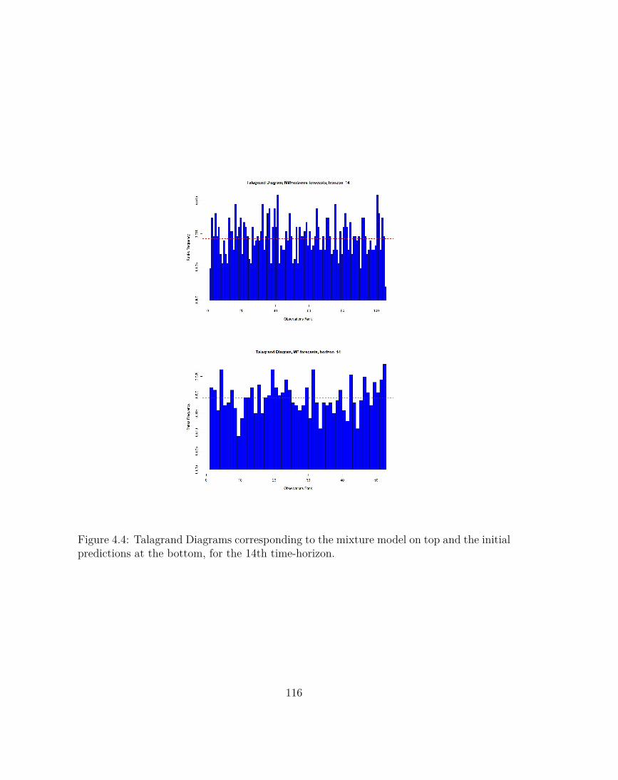
Figure 4.4: Talagrand Diagrams corresponding to the mixture model on top and the initialpredictions at the bottom, for the 14th time-horizon.

116

Figure 4.5: Talagrand Diagrams corresponding to the mixture model when separatingextreme values by boards and at right also by horizon. On top and the initial predictionsat the bottom, for the time-horizons 8, 9 and 10 respectively.

117

Figure 4.6: Talagrand Diagrams corresponding to the mixture model when separatingextreme values by boards and at right also by horizon. On top and the initial predictionsat the bottom, for the time-horizons 11, 12 and 13 respectively.

118

Figure 4.7: Talagrand Diagrams corresponding to the mixture model when separatingextreme values by boards and at right also by horizon. On top and the initial predictionsat the bottom, for the 14th time-horizon.

119

Figure 4.8: Talagrand Diagrams corresponding to the mixture model when separatingextreme values by time-horizon packages and by month on top and the initial predictionsat the bottom, for the time-horizons 8, 9 and 10 respectively.

120

Figure 4.9: Talagrand Diagrams corresponding to the mixture model when separatingextreme values by time-horizon packages and by month on top and the initial predictionsat the bottom, for the time-horizons 11, 12 and 13 respectively.

121

Figure 4.10: Talagrand Diagrams corresponding to the mixture model when separatingextreme values by boards and at right also by horizon on top and the initial predictionsat the bottom, for the 14th time-horizon.

122

Case of the Extreme Values given by the 1st and 51strankWe will present here the results obtained when we consider as extreme values only the valuesissues of the Ranks 1 and 51. The most important thing changing is the number of the extremevalues: 1129 against 3566 when we consider also the 2nd the 50th rank in the extreme valuesdata.

Horizon Rank 1 Rank 51 Rank 1 + Rank 515 67 93 1606 58 68 1267 52 64 1168 42 65 1079 46 51 9710 54 57 11111 51 52 10312 52 56 10813 51 49 10014 46 55 101All 519 610 1129

Table 4.7: If we consider as extreme values only the values coming from the rank 1 and51 we will have the number of values in this table.

From the AIC point of view the best models is the 15th and the 16th. But even when wechoose the one less separating our data (the 16th) - by months, by ranks and by packages oftime-horizons- we still have certain classes with not enough data. We will have to go up tothe model 23rd to have enough data in all the classes for estimating the parameters of theGEV distributions. The model 23 splits extreme values: by rank (1st and 51st) and by horizonpackages (5, 6, 7 ∈ PH1, 8, 9, 10 ∈ PH2, 11, 12, 13, 14 ∈ PH3)When we compute all the scores we studied in the thesis, we notice an improvement from aCRPS point of view and a loss from the RMSE point of view of the same order as from the casewhere we considered the rank 2 and 50 as well as extreme valuesThe Talagrand Diagram (see Fig 4) was the reason we studied this case of extreme values selection(1 and 51 ranks) but we notice the extreme right side of the diagram still has very little valuesrepresented - this is why the case is only presented in the Appendix. This is also confirmed bythe quantile representation, Table 4.9.

123

Horizon CRPSpot CRPSReli CRPS MAE RMSE R25 0.5859 0.0040 0.5899 1.248 1.683 0.9686 0.7383 0.0031 0.7413 1.545 2.074 0.9527 0.9062 0.0037 0.9098 1.880 2.493 0.9328 1.0498 0.0026 1.0523 2.159 2.843 0.9139 1.1794 0.0022 1.1816 2.397 3.127 0.89710 1.2937 0.0023 1.2960 2.630 3.406 0.87911 1.3762 0.0024 1.3785 2.796 3.617 0.86712 1.4285 0.0036 1.4321 2.924 3.763 0.85613 1.4761 0.0025 1.4786 3.001 3.847 0.84814 1.4864 0.0025 1.4889 3.043 3.903 0.845

Table 4.8: The different scores by time-horizon, for the forecasts obtained when creating amixture model: BMM for the central part of the distribution and 6 different GEV functionsfor the two tails and three horizon packages. We notice an improvement from a CRPSpoint of view and a loss from the RMSE point of view of the same order as from the casewhere we considered the rank 2 and 50 as well as extreme values.

124

Figure 4.11: We consider as extreme values only the values issues of the Ranks 1 and 51.From the AIC point of view the best models is the 15th and the 16th. But even when wechoose the one less separating our data (the 16th) - by months, by ranks and by packagesof time-horizons- we still have certain classes with not enough data. We will have to goup to the model 23rd to have enough data in all the classes for estimating the parametersof the GEV distributions. The model 23 splits extreme values: by rank (1st and 51st) andby horizon packages (5, 6, 7 ∈ PH1, 8, 9, 10 ∈ PH2, 11, 12, 13, 14 ∈ PH3)

125

Figure 4.12: On top: Talagrand Diagrams corresponding to the mixture model (whenthe extreme values are those corresponding to the rank 1 and 51) indicated by the AICcriterion (the first where we have enough values for all the classes to estimate the GEVparameters). At the bottom, rank diagram for the initial predictions, for the time-horizons5, 6 and 7 respectively. We remarque the same problem for the 51st rank, proofed also bythe Table of the right quantiles bellow.

126

H Model Q1 Q99 Q2 Q98 Q5 Q95 Q10 Q905 Mixt .0240 .0000 .0438 .0078 .0602 .0233 .0985 .1061

MF .0363 .0493 .0583 .0843 .0781 .1117 .1323 .17686 Mixt .0240 .0048 .0370 .0192 .0569 .0418 .0960 .1180

MF .0309 .0357 .0535 .0617 .0748 .0816 .1276 .15647 Mixt .0247 .0000 .0515 .0089 .0638 .0268 .1208 .0933

MF .0254 .0377 .0494 .0597 .0734 .0879 .1290 .15998 Mixt .0151 .0014 .0309 .0206 .0467 .0412 .0968 .1120

MF .0192 .0357 .0405 .0536 .0659 .0769 .1312 .14779 Mixt .0151 .0055 .0323 .0227 .0495 .0515 .1031 .1134

MF .0234 .0289 .0467 .0488 .0701 .0742 .1271 .147810 Mixt .0144 .0069 .0330 .0275 .0509 .0453 .1025 .1093

MF .0282 .0296 .0509 .0502 .0702 .0729 .1279 .147211 Mixt .0117 .0062 .0289 .0220 .0502 .0468 .0970 .1191

MF .0255 .0248 .0434 .0496 .0654 .0695 .1246 .134212 Mixt .0110 .0090 .0289 .0227 .0482 .0468 .0964 .1274

MF .0269 .0310 .0455 .0475 .0654 .0723 .1198 .135713 Mixt .0159 .0021 .0372 .0172 .0524 .0420 .1006 .1116

MF .0262 .0241 .0496 .0482 .0669 .0731 .1165 .128914 Mixt .0200 .0014 .0490 .0207 .0648 .0414 .1145 .0931

MF .0221 .0283 .0434 .0524 .0593 .0731 .1214 .1345

Table 4.9: The quantiles 1%, 2%, 5%, 95%, 98%, 99%, for the initial MF forecasts and forthe mixture model. We are in the case where the extreme values are those correspondingto the ranks 1, 51 and where the parameters of the GEV functions are computed separatelyby and by rank and by package of time-horizons.

127

128

List of Figures

1.1 Daily electricity loads versus the national average temperature from September 1,1995 to August 31, 2004, at 9 AM. . . . . . . . . . . . . . . . . . . . . . . . . . . 23

1.2 The map of the Meteo France stations. . . . . . . . . . . . . . . . . . . . . . . . . 251.3 Figures corresponding to initial predictions. On top, the curve of realizations

and the one of the average predicted temperature. At the bottom, the curves oftemperatures for one day, for all the 14 horizons time. . . . . . . . . . . . . . . . 26

1.4 Possible situations for the Talagrand Diagram . . . . . . . . . . . . . . . . . . . . 331.5 Each point on the ROC curve represents a sensitivity/specificity pair correspond-

ing to a particular decision threshold. . . . . . . . . . . . . . . . . . . . . . . . . 35

3.1 Errors densities and empirical distributions of all the extreme values included, allranks included (rank 1 and rank 2 with rank 50 and rank 51, and also rank 1 andrank 2 with -rank 50 and -rank 51) and left ranks and right ranks separated. . . 77

3.2 At the top: Errors densities by time-horizon, all ranks included. We notice thedensities shapes look alike but theirs mean are divided between 0 and 1. At thebottom errors densities by time-horizon, by ranks, separating left and right. Wenotice that the densities of the left values, for different horizons are much morealike than the densities of the different horizons for the right values. . . . . . . . 82

3.3 Errors densities and GEV distributions of the left extreme values for the four season. 853.4 Errors densities and GEV distributions of the right extreme values for the four

season. . . . . . . . . . . . . . . . . . . . . . . . . . . . . . . . . . . . . . . . . . . 863.5 The GEV parameters for the values coming from the B51. We can see that the

shape parameter (the most important as it decides of the case of the GEV functionwe are in) has a small variation from a season to another and it is always negative. 87

3.6 The GEV parameters for the values coming from the B1. We can see that theshape parameter (the most important as it decides of the case of the GEV functionwe are in) has a very small variation from a season to another and it is alwaysnegative. . . . . . . . . . . . . . . . . . . . . . . . . . . . . . . . . . . . . . . . . . 88

3.7 The errors densities and their corresponding GEV distributions for the right ex-treme values for three packages of horizons. The first package, with the 5th, 6thand 7th horizon is the one fitting less good the distribution. . . . . . . . . . . . . 89

129

3.8 From the AIC point of view the best models is the 15th but it is correspondingto a very large number of parameters as it separates the extreme values by day.The estimation parameters classes does not respect the condition of the numberof values large enough. The first model respecting it is the 18th and it separatesthe extreme values by Package of time-horizon, by month and by rank. . . . . . . 90

3.9 Talagrand Diagrams corresponding to the mixture model (with the GEV param-eters estimated by tail and by season) on top and the initial predictions at thebottom, for the time-horizons 5, 6 and 7 respectively. . . . . . . . . . . . . . . . . 92

3.10 Talagrand Diagrams corresponding to the mixture model - that separates extremevalues by tail and for the right tail, by time-horizon - on top and the initialpredictions at the bottom, for the time-horizons 5, 6 and 7 respectively. . . . . . 94

3.11 Talagrand Diagrams corresponding to the mixture model (GEV parameters esti-mated by tail, by month and by package of time-horizon) on top and the initialpredictions at the bottom, for the time-horizons 5, 6 and 7 respectively. . . . . . 95

4.1 Errors densities and their corresponding GEV distributions for the left extremevalues for three packages of horizons. We notice that the GEV fits good enoughthe observed distributions, less god for the 2nd package but in the adjustment testfor the three cases H0 is not rejected (H0 : assumes that the values in the twodistributions come from a single distribution.) . . . . . . . . . . . . . . . . . . . . 113

4.2 Talagrand Diagrams corresponding to the mixture model on top and the initialpredictions at the bottom, for the time-horizons 8, 9 and 10 respectively. . . . . . 114

4.3 Talagrand Diagrams corresponding to the mixture model on top and the initialpredictions at the bottom, for the time-horizons 11, 12 and 13 respectively. . . . 115

4.4 Talagrand Diagrams corresponding to the mixture model on top and the initialpredictions at the bottom, for the 14th time-horizon. . . . . . . . . . . . . . . . . 116

4.5 Talagrand Diagrams corresponding to the mixture model when separating extremevalues by boards and at right also by horizon. On top and the initial predictionsat the bottom, for the time-horizons 8, 9 and 10 respectively. . . . . . . . . . . . 117

4.6 Talagrand Diagrams corresponding to the mixture model when separating extremevalues by boards and at right also by horizon. On top and the initial predictionsat the bottom, for the time-horizons 11, 12 and 13 respectively. . . . . . . . . . . 118

4.7 Talagrand Diagrams corresponding to the mixture model when separating extremevalues by boards and at right also by horizon. On top and the initial predictionsat the bottom, for the 14th time-horizon. . . . . . . . . . . . . . . . . . . . . . . 119

4.8 Talagrand Diagrams corresponding to the mixture model when separating extremevalues by time-horizon packages and by month on top and the initial predictionsat the bottom, for the time-horizons 8, 9 and 10 respectively. . . . . . . . . . . . 120

4.9 Talagrand Diagrams corresponding to the mixture model when separating extremevalues by time-horizon packages and by month on top and the initial predictionsat the bottom, for the time-horizons 11, 12 and 13 respectively. . . . . . . . . . . 121

130

4.10 Talagrand Diagrams corresponding to the mixture model when separating extremevalues by boards and at right also by horizon on top and the initial predictions atthe bottom, for the 14th time-horizon. . . . . . . . . . . . . . . . . . . . . . . . . 122

4.11 We consider as extreme values only the values issues of the Ranks 1 and 51. Fromthe AIC point of view the best models is the 15th and the 16th. But even whenwe choose the one less separating our data (the 16th) - by months, by ranks andby packages of time-horizons- we still have certain classes with not enough data.We will have to go up to the model 23rd to have enough data in all the classes forestimating the parameters of the GEV distributions. The model 23 splits extremevalues: by rank (1st and 51st) and by horizon packages (5, 6, 7 ∈ PH1, 8, 9, 10∈ PH2, 11, 12, 13, 14 ∈ PH3) . . . . . . . . . . . . . . . . . . . . . . . . . . . . 125

4.12 On top: Talagrand Diagrams corresponding to the mixture model (when the ex-treme values are those corresponding to the rank 1 and 51) indicated by the AICcriterion (the first where we have enough values for all the classes to estimate theGEV parameters). At the bottom, rank diagram for the initial predictions, forthe time-horizons 5, 6 and 7 respectively. We remarque the same problem for the51st rank, proofed also by the Table of the right quantiles bellow. . . . . . . . . . 126

131

132

List of Tables

3.1 The most common laws distributed by attraction domain . . . . . . . . . . . . . 643.2 The number of values included in our study of the extreme values. . . . . . . . . 763.3 The p-values for the KS test, at the 5% significance level with H0 : the values of the

time-horizon i and the ones from the time-horizon j (with i 6= j) belong to the samedistribution. . . . . . . . . . . . . . . . . . . . . . . . . . . . . . . . . . . . . . . . 83

3.4 The KS p−value tests, when taking out values from each horizon, one at the timeand comparing the distribution of what is resting with the distribution of whatwe took out. For B51 H0 is rejected, at a 5% significance level for all the horizonsexcepting horizons 6, 8 and 14. For B1 H0 is not rejected and that is for all thehorizons excepting horizons 11 and 13. This results confirm the test horizon byhorizon. . . . . . . . . . . . . . . . . . . . . . . . . . . . . . . . . . . . . . . . . . 84

3.5 The estimations parameters by season, to notice the shape parameter that isalways negative, corresponding to a GEV distribution of Weibull type. . . . . . . 84

3.6 The different scores by time-horizon, for the forecasts obtained when creating amixture model: BMM for the central part of the distribution and GEV functionsfor the tails, having their parameters estimated by tail and by season. . . . . . . 91

3.7 The different scores by time-horizon, for the initial MF forecasts . . . . . . . . . 913.8 The different scores by time-horizon, for the forecasts obtained when simulating

with the mixture model that separates extreme values by tail and for the righttail, by time-horizon. . . . . . . . . . . . . . . . . . . . . . . . . . . . . . . . . . . 93

3.9 The different scores by time-horizon, for the forecasts obtained when simulatingwith the mixture model selected by the AIC criterion: GEV parameters estimatedby tail, by month and by horizon package. We have good scores, we improve theCRPS for all the period. . . . . . . . . . . . . . . . . . . . . . . . . . . . . . . . . 97

3.10 The quantiles 1%, 2%, 5%, 95%, 98%, 99%, for the initial MF forecasts and forthe mixture models when we compute the parameters separately by month andby package of time-horizons. . . . . . . . . . . . . . . . . . . . . . . . . . . . . . . 98

4.1 The different scores by time-horizon, for the MF (initial) forecasts. . . . . . . . . 1104.2 The different scores by time-horizon, for the forecasts obtained with the BMM for

the entire distribution. . . . . . . . . . . . . . . . . . . . . . . . . . . . . . . . . . 1104.3 The number of values, by time-horizon and by season included in our study of the

extreme values. . . . . . . . . . . . . . . . . . . . . . . . . . . . . . . . . . . . . . 111

133

4.4 The p-values corresponding to the KS test where H0 is the hypothesis that theextreme values (for board = 1) of the j-time horizon can be consider as comingfrom the same distribution as the values from all the time-horizons other than j. 111

4.5 The p-values corresponding to the KS test where H0 is the hypothesis that theextreme values (for board = 51) of the j-time horizon can be consider as comingfrom the same distribution as the values from all the time-horizons other than j.W notice all the p− values, excepting horizon 6 and 14, are smaller than 0.05 sowe can reject H0: for the rank 51 values, the extreme values coming from differenthorizons can not be considered as coming from the same distribution. . . . . . . 112

4.6 The different scores by time-horizon, for the forecast obtained when creating amixture model: BMM for the central part of the distribution and EVT for the tails112

4.7 If we consider as extreme values only the values coming from the rank 1 and 51we will have the number of values in this table. . . . . . . . . . . . . . . . . . . . 123

4.8 The different scores by time-horizon, for the forecasts obtained when creating amixture model: BMM for the central part of the distribution and 6 different GEVfunctions for the two tails and three horizon packages. We notice an improvementfrom a CRPS point of view and a loss from the RMSE point of view of the sameorder as from the case where we considered the rank 2 and 50 as well as extremevalues. . . . . . . . . . . . . . . . . . . . . . . . . . . . . . . . . . . . . . . . . . . 124

4.9 The quantiles 1%, 2%, 5%, 95%, 98%, 99%, for the initial MF forecasts andfor the mixture model. We are in the case where the extreme values are thosecorresponding to the ranks 1, 51 and where the parameters of the GEV functionsare computed separately by and by rank and by package of time-horizons. . . . . 127

134

Bibliography

[AF97] J. ALDRICH and R.A. FISHER, The making of maximum likelihood, StatisticalScience 12 (1997), 162 –176.

[BBW+07] R. BUIZZA, J.R. BIDLOT, M. WEDI, N. FUENTES, M. HAMRUD, G. HOLT,and F. VITART, The new ecmwf vareps (variable resolution ensemble predictionsystem), Q.J.R. Meterological Society 133 (2007), 681–695.

[BCG00] C. BIERNACKI, G. CELEUX, and G. GOVAERT, Assessing a mixture model forclustering with the integrated completed likelihood, IEEE transactions on patternanalysis and machine intelligence 22 (2000), 719–725.

[BCHY09] T. BENAGLIA, D. CHAVEAU, D.R. HUNTER, and D.S. YOUNG, mixtools: Anr package for analyzing finite mixture models, Journal of Statistical Software 32(2009).

[BDR05] A. BRUHNS, G. DEURVEILHER, and J-S. ROY, A non-linear regression modelfor mid-term load forecasting and improvements in seasonality, 15th PSCC, Liege„2005.

[BER] J.M. BERNARDO, The concept of exchangeability and its applications, Far East J.Mathematical Sciences Special volume, 111–121.

[BER72] L. Von. BERTALANFFY, The history and satus of general system theory, TheAcademy of Management Journal 15 (1972), 407– 426.

[BHG04] C.N. BEHRENS, LOPES H.F., and D. GAMERMAN, Bayesian analysis of extremeevents with threshold estimation., Statistical Modelling 4 (3) (2004), 227–244.

[BLA09] P. BLANC, Ensemble-based uncertainty prediction for deterministic 2 m tempera-ture forecasts, Master’s thesis, Faculty of Science University of Bern, 2009.

[BRI50] G. W. BRIER, Verification of forecasts expressed in terms of probability, MonthlyWeather Review 78 (1950), 1–3.

[BS07] William BUA and Bonnie SLAGEL, La prévision d’ensemble expliquée, 2007.

135

[BTV96] J. BEIRLANT, J. TEUGELS, and P. VYNCKIER, Practical analysis of extremevalues, Leuven University Press (1996).

[CB09] J. CARREAU and Y. BENGIO, A hybrid pareto model for asymmetric fat-taileddata: the univariate case., Extremes 12 (1) (2009), 53–76.

[CD10] J. COLLET and V. DORDONNAT, Aléas physiques perturbant la gestion offre-demande : état de l’art complément à la feuille de route du pôle aléas, Tech. report,EDF R&D, 2010.

[COL01] S. COLES, An introduction to statistical modeling of extreme values, Springer, 2001.

[COL08] J. COLLET, Note d’opportunité d’un partenariat et d’une thèse sur l’utilisationstatistique de résultats de modèles physiques, Tech. report, EDF R&D, 2008.

[CWS+08] B. CASATI, L.J. WILSON, D. B. STEPHENSON, P. NURMI, A. GHELLI, andM. POCERNICH, Forecasts verification: current status and future directions, Me-teorological Applications 15 (2008), 3–18.

[DC10] V. DORDONNAT and J. COLLET, Méthodes de prévision en loi : état de l’art,Tech. report, EDF R&D, 2010.

[DDHDV01] J. DANIELSSON, L. DE HAAN, and C. G. DE VRIES, Using a bootstrap method tochoose the sample fraction in tail index estimation, Journal of Multivariate Analysis76 (2001), 226–248.

[DGT98] F. DIEBOLD, T. GUNTHER, and A. TAY, Evaluating Density Forecasts withApplications to Financial Risk Management, Internationa1 Economic Review 39(1998), no. 4, 863–883.

[DKO+08] V DORDONNAT, S.J. KOOPMAN, M. OOMS, A. DESSERTAINE, and J. COL-LET, An hourly periodic state space model for modelling French national electricityload, International Journal of Forecasting 24 (2008), no. 4, 566–587.

[DLR77] A. P. DEMPSTER, N. M. LAIRD, and D. B. RUBIN, Maximum likelihood fromincomplete data via the em algorithm, Journal of the Royal Statistical Society 39(1977), 1–38.

[DOC02] IFS DOCUMENTATION, The ensemble prediction system, Tech. report, ECMWF,2002.

[DOC06] , Part v: The ensemble prediction systems, Tech. report, ECMWF, 2006.

[DOR09] V. DORDONNAT, State-space modelling for high frequency data. three applicationsto french national electricity load, Ph.D. thesis, Vrije Universiteit Amsterdam, 2009.

[DU07] J. DU, Uncertainty and ensemble forecast, Tech. report, SREF Development Team,EMC/NCEP/NOAA, 2007.

136

[EAT08] S. EL ADLOUNI and OUARDA T.B., Comparaison des méthodes d’estimation desparamètres du modèle gev non stationnaire, Journal of Water Science 21 (2008),35–50.

[EKM97] P. EMBRECHTS, C. KLUPPELBERG, and T. MIKOSCH, Modelling extremalevents for insurance and finance, 1997.

[EMP11] G. EVIN, J. MERLEAU, and L. PERREAULT, Two-component mixtures of nor-mal, gamma, and gumbel distributions for hydrological applications, Water Resour.Res. 47 (2011).

[ENM]

[EPS69] E. S. EPSTEIN, Stochadtic dynamic prediction, Tellus 21 (1969), 739–759.

[FFS06] V. FORTIN, A.C. FAVRE, and M. SAID, Probabilistic forecasting from ensembleprediction systems: Improving upon the best-member method by using a differentweight and dressing kernel for each member, Q. J. R. Meteorol. Soc. 132 (2006),1349 –1369.

[FHR02] A. FRIGESSI, O. HAUG, and H. RUE, A dynamic mixture model for unsupervisedtail estimation without threshold selection, Extremes 5 (3) (2002), 219–235.

[FRGS09] C. FRALEY, A. E. RAFTERY, T. GNEITING, and J. M. SLOUGHTER, ensem-blebma: An r package for probabilistic forecasting using ensembles and bayesianmodel averaging, Tech. report, Department of Statistics University of Washington,2009.

[GAA10] COLLET J. GOGONEL A. and BAR-HEN A., Utilisation des méthodes ensemblistepour la prévision d’électricité, Congrès de la Société Marocaine de MathématiquesAppliquées, Rabat, 2010.

[GAA11] , Ensemble prediction systems of temperature for the french electric system,International Symposium on Forecasting, Prague, 2011.

[GAA12a] , Improvement of extreme temperatures probabilistic short-terme forecasting,International Conference on Computational Statistics, Limassol, 2012.

[GAA12b] , Improvement of extreme temperatures probabilistic short-terme forecasting,Workshop on Stochastic Weather Generators, Roscoff, 2012.

[GAAer] , Implementation of ensemble prediction systems post-processing methods,for the electric system management, The World Statistics Congress (ISI), Dublin,2011, Poster.

137

[GBL+05] G. GIEBEL, J. BADGER, L. LANDBERG, H-A NIELSEN, T-S NIELSEN,H. MADSEN, K. SATTLER, H. FEDDERSEN, H. VEDEL, J. TOFTING,L. KRUSE, and L. VOULUND, Wind power prediction using ensembles, Tech.report, Risk National Laboratory Roskilde Denmark, 2005.

[GCAA12] COLLET J. GOGONEL-CUCU A. and BAR-HEN A., Statistical post-processingmethods implemented on the outputs of the ensemble prediction systems of tempera-ture, for the french electric system management, Journal Case Studies in Business,Industry and Government Statistics, Bentley University (CSBIGS) 5(2) (2012).

[GDC97] E. GASSIAT and D. DACUHNA-CASTELLE, Estimation of the number of com-ponents in a mixture., Bernoulli 3 (1997), 279–299.

[GIL09] E. GILLELAND, An introduction to the analysis of extreme values using r andextremes, Graybill VIII, 2009.

[GIL12] , Package ’verification’, Tech. report, NCAR - Research Application Pro-gram, 2012.

[GRWG05] T. GNEITING, A. E. RAFTERY, A.H. WESTVELD, and T. GOLDMAN, Cali-brated probabilistic forecasting using ensemble model output statistics and minimumcrps estimation, Monthly Weather Review 133 (2005), 1098–1118.

[GYH+11] M. GHIL, P. YIOU, S. HALLEGATTE, BD. MALAMUD, and P.NAVEAU, Ex-treme events: dynamics, statistics and prediction, Tech. report, Copernicus Publi-cations, 2011.

[Hag10] Renate Hagedorn, Post-processing of eps forecasts, 2010.

[HER00] H. HERSBACH, Decomposition of the Continuous Ranked Probability Score forEnsemble Prediction Systems, Weather and Forecasting 15 (2000), no. 5, 559–570.

[HOU07] P. HOUTEKAMER, Rudiments de la prévision d’ensemble, Tech. report, Sémi-naires RPN, 2007.

[Ins06] SAS Institute, The GLMSelect procedure : Stepwise selection(stepwise), 2006.

[JA05] L JAGER and WELLNER J A., A new goodness-of-fit test: the reversed Berk-Jonesstatistic, Tech. Report TR443, Department of Statistics, University of Washington,2005.

[JMW09] S. JENSEN, B.B. McSHANE, and A.J. WYNER, Hierarchical bayesian modellingof hitting performances in baseball, Bayesian Analysis 4 (2009), 631–652.

[JS03] I. T. JOLLIFFE and D. B. STEPHENSON, Forecast verification: A practitioner’sguide in atmospheric science., Wiley (2003).

138

[JS07] , Proper scores for probability forecasts can never be equitable, AmericanMeteorological Society (2007).

[KA09] D. KORTSCHAK and H. ALBRECHER, Asymptotic results for the sum of depen-dent non-identically distributed random variables, Methodology and Computing inApplied Probability 11 (2009), 279–306.

[KAT08] R.W. KATZ, Background on extreme value theory with emphasis on climate ap-plications, Tech. report, Institute for Study of Society and Environment NationalCenter for Atmospheric Research Boulder, CO USA, 2008.

[KB78] R. KOENKER and G. BASSETT, Regression Quantiles, Econometrica 46 (1978),no. 1, 33–50.

[LEI74] C. E. LEITH, Theoretical skill of monte carlo forecasts, Monthly Weather Review102 (1974), 409–418.

[LLR83] R. LEADBETTER, G. LINDGREN, and H. ROOTZEN, Extremes and relatedpropertiesof random sequences and processes, 1983.

[MAL05] V. MALLET, Estimation de l’incertitude et prévision d’ensemble avec un modèlede chimie-transport, Ph.D. thesis, Ecole nationale des ponts et chaussées, 2005.

[MAL08] , Prévision d’ensemble, Tech. report, INRIA Roquencourt, 2008.

[MBPP96] F. MOLTENI, R. BUIZZA, T. PALMER, and T. PETROLIAGIS, The ecmwf en-semble prediction system, Q.J.R. Meterological Society 122 (1996), 73–119.

[MF00] A. J. McNEIL and R. FREY, Estimation of tail-related risk measures for het-eroscedastic financial time series: An extreme value approach, Journal of EmpiricalFinance 7 (2000), 271–300.

[ML04] B. MENDES and H.F LOPES, Data driven estimates for mixtures, ComputationalStatistics and Data Analysis 47 (3) (2004), 583–598.

[MMP]

[MP07] LEUTBECHER M. and T.N. PALMER, Ensemble forecasting, Tech. report,ECMWF, 2007.

[MRT09] V. MARIMOUTOU, B. RAGGAD, and A. TRABELSI, Extreme value theory andvalue at risk: Application to oil market, Energy Economics 31 (2009), 519–530.

[MS97] A.J. MCNEIL and T. SALADIN, The peaks over thresholds method for estimatinghigh quantiles of loss distributions, Tech. report, Departement Mathematik ETHZentrum, Zurich, 1997.

139

[MSL+11] A. MACDONALD, C.J. SCARROTT, D. LEE, B. DARLOW, M. REALE, andG. RUSSELL, A flexible extreme value mixture model, Computational Statisticsand Data Analysis 55 (2011), 2137–2157.

[NAS84] S.G. NASH, Newton-type minimization via the lanczos method, SIAM J. 21 (1984),770–778.

[NJ11] P. NORTHROP and P. JONATHAN, Threshold modelling of spatially dependentnon-stationary extremes with application to hurricane-induced wave heights, Envi-ronmetrics (2011).

[NPDC07] M. NOGAJ, S. PAREY, and D. DACUNHA-CASTELLE, Non-stationary extrememodels and a climatic application, Nonlinear Processes in Geophysics 14 (2007),305–316.

[NUR07] P. NURMI, Mixture models, Tech. report, Helsinki Institute for Information Tech-nology, 2007.

[oYSS12] International Conference of Young Scientists and Students (eds.), Statistical post-processing methods and their implementation on the ensemble prediction systemsfor forecasting temperature in the use of the french electric consumption., Depart-ment of Information Systems Sevastopol National Technical University, Sevastopol,Ukraine, 2012.

[PBM+07] T.N. PALMER, R. BUIZZA, LEUTBECHER M., R. HAGEDORN, T. JUNG,M. RODWELL, F. VITART, J. BERNER, E. HAGEL, A. LAWRENCE, F. PAP-PENBERGER, Y-Y. PARK, L. VON BREMEN, and I. GILMOUR, The ensem-ble prediction system - recent and ongoing developments, Tech. report, ResearchDepartment of ECMWF and Hungarian Met Service and Budapest, Korea Me-teorological Administration, Seoul ForWind, Center for Wind Energy Research,Germany, Merrill Lynch, London, 2007.

[PER03] A. PERSSON, User guide to ecmwf forecast products, Tech. report, ECMWF, 2003.

[PET08] T. PETIT, Evaluation de la performance de prévisions hydrologiques logiquesd’ensemble issues de prévisions météorologiques d’ensemble, Ph.D. thesis, FacultéDes Sciences Et De Génie Université Laval Québec, 2008.

[PIC07] F. PICARD, An introduction to mixture models, Tech. report, Laboratoire Statis-tique et Genome, UMR CNRS 8071 - INRA 1152 - Univ. d’Evry, France, 2007.

[POC10] M. POCERNICH, Verification package: examples using weather forecasts., Tech.report, National Center for Atmospheric Sciences (NCAR), 2010.

[RAG09] B. RAGGAD, Fondements de la théorie des valeurs extrêmes, ses principales ap-plications et son apport à la gestion des risques du marché pétrolier, Mathematicsand Social Sciences 186 (2009), 29–63.

140

[RGBP04] A.E. RAFTERY, T. GNEITING, F. BALABDAOUI, and M. POLAKOWSKI,Using bayesian model averaging to calibrate forecast ensembles, Physical Review(2004), 20.

[ROB] C. Y. ROBERT, Automatic declustering of rare events, Université Lyon 1 (ISFA).

[ROSG09] M. RIBATET, T.B. OUARDA, E. SAUQUET, and J.M. GRESILLON, Modelingall exceedances above a threshold using an extremal dependence structure: Infer-ences on several flood characteristics, Water Ressources Research 45 (2009).

[RS02] ROULSTON and SMITH, Combining dynamical and statistical ensembles, Tellus55A (2002), 16–30.

[SCH78] G. SCHWARTS, Estimating the dimension of a model. annals of statistics, Annalsof Statistics 6 (1978), 461–464.

[SDH+07] J. SCHAAKE, J. DEMARGNE, R. HARTMAN, M. MULLUSKY, E. WELLES,L. WU, H. HERR, X. FAN, and D. J. SEO, Precipitation and temperature en-semble forecasts from single-value forecasts, Hydrology and Earth System SciencesDiscussions 4 (2007), 655 – 717.

[STE12] A. STEPHENSON, Package ’evd’: Functions for extreme value distributions., Tech.report, R cran, 2012.

[Sur04] Mémento de la sûreté du système électrique, édition 2004, Tech. report, Réseau deTransport d’Électricité, 2004.

[SWa06] S. SAHA, W. WANG, and H.-L. PAN and, The ncep climate forecast system, Amer-ican Meteorological Society (2006), 3483–3517.

[SWB89] H.R. STANSKI, L.H. WILSON, and W. R. BURROWS, Survey of common ver-ification methods in meteorology, Tech. report, Environement Canada, Service del’environement atmosphérique., 1989.

[TAO06] A. TANCREDI, C. ANDERSON, and A. O’HAGAN, Accounting for threshold un-certainty in extreme value estimation., Extremes 9 (2) (2006), 87–106.

[TL00] S. TADJUDIN and D.A. LANDGREBE, Robust parameter estimation for mixturemodel, IEEE Transactions on Geoscience and Remote Sensing 38 (2000), 439–455.

[VER06] J. VERDUN, Introduction au filtrage de kalman, Tech. report, Ecole Nationale desSciences Géographiques, Département Positionnement Terrestre et Spatial, 2006.

[WB05] X. WANG and C.H. BISHOP, Improvement of ensemble reliability with a new dress-ing kernel., Q. J. R. Meteorol. Soc. 131 (2005), 965–986.

[WL98] J.S. WHITAKER and A. F. LOUGHE, The relationship between ensemble spreadand ensemble mean skill, Monthly Weather Review 126 (1998), 3292 – 3302.

141

[WZZ00] B. WANG, X. ZOU, and J. ZHU, Data assimilation and its applications, Proceed-ings of the National Academy of Sciences, 2000.

142