statistical power and optimal design in experiments in...

Statistical Power and Optimal Design in Experiments in Which Samples ofParticipants Respond to Samples of Stimuli

Jacob WestfallUniversity of Colorado Boulder

David A. KennyUniversity of Connecticut

Charles M. JuddUniversity of Colorado Boulder

Researchers designing experiments in which a sample of participants responds to a sample of stimuli arefaced with difficult questions about optimal study design. The conventional procedures of statisticalpower analysis fail to provide appropriate answers to these questions because they are based on statisticalmodels in which stimuli are not assumed to be a source of random variation in the data, models that areinappropriate for experiments involving crossed random factors of participants and stimuli. In this article,we present new methods of power analysis for designs with crossed random factors, and we give detailed,practical guidance to psychology researchers planning experiments in which a sample of participantsresponds to a sample of stimuli. We extensively examine 5 commonly used experimental designs,describe how to estimate statistical power in each, and provide power analysis results based on areasonable set of default parameter values. We then develop general conclusions and formulate rules ofthumb concerning the optimal design of experiments in which a sample of participants responds to asample of stimuli. We show that in crossed designs, statistical power typically does not approach unityas the number of participants goes to infinity but instead approaches a maximum attainable power valuethat is possibly small, depending on the stimulus sample. We also consider the statistical merits ofdesigns involving multiple stimulus blocks. Finally, we provide a simple and flexible Web-based powerapplication to aid researchers in planning studies with samples of stimuli.

Keywords: statistical power, experimental design, optimal design, stimulus sampling, mixed models

Studies in which samples of participants respond to samples ofstimuli in various experimental conditions are ubiquitous in ex-perimental psychology. In studies of memory, participants oftenmemorize lists of words that are drawn from a larger corpus ofwords. In studies of social cognition, participants often makejudgments about sets of faces or read vignettes about hypotheticalpersons. In studies of emotion, participants are often exposed tophotographs or film clips of emotion-provoking scenes. In all ofthese examples, the particular individual stimuli used are not ofintrinsic theoretical interest, except insofar as they instantiate thegeneral categories to which they belong (e.g., monosyllabic com-mon words; African American male facial photos). What aretypically of interest are any differences in the responses given in

the different conditions to those stimuli (e.g., better word memoryin one condition than another; more negative judgments of AfricanAmerican faces than of White faces).

In designing such studies, researchers are faced with a variety ofdesign decisions concerning participants, stimuli, and the specificsof the design used. There is a series of decisions to be made aboutparticipants: Should one sample participants broadly to increasegeneralization, or should one restrict the sample of participantsused to maximize power? Should one use a design where partic-ipants are only in one condition, or should a within-participantdesign be used? And finally, how many participants should be run?These are decisions that researchers realize have consequences forstatistical power and the kinds of generalizations that are permittedfrom the subsequently collected data.

Similar decisions are made, although too often in a cursorymanner, about stimuli: How variable should the stimuli be? Howmany stimuli should be used? And should stimuli be different inthe different conditions or should the same stimuli be used acrossconditions? Unfortunately, researchers often do not realize thatthese decisions also have major consequences for statistical powerand the kinds of generalizations that they permit. All too often,these decisions about stimuli are based more on the traditionalpractices within an experimental paradigm rather than well-thought-out principles about the optimal design of experiments.

This article focuses on issues of statistical power and optimaldesign in experiments in which samples of participants respond to

This article was published Online First August 11, 2014.Jacob Westfall, Department of Psychology and Neuroscience, Univer-

sity of Colorado Boulder; David A. Kenny, Department of Psychology,University of Connecticut; Charles M. Judd, Department of Psychology,University of Colorado Boulder.

We thank Markus Brauer, Deborah Kashy, John Lynch, DominiqueMuller, Gary McClelland, Thom Baguley, and members of the Stereotyp-ing and Prejudice Lab at the University of Colorado for helpful commentson an earlier version of this article.

Correspondence concerning this article should be addressed to JacobWestfall, Department of Psychology and Neuroscience, University ofColorado, Boulder, CO 80309-0345. E-mail: [email protected]

Thi

sdo

cum

ent

isco

pyri

ghte

dby

the

Am

eric

anPs

ycho

logi

cal

Ass

ocia

tion

oron

eof

itsal

lied

publ

ishe

rs.

Thi

sar

ticle

isin

tend

edso

lely

for

the

pers

onal

use

ofth

ein

divi

dual

user

and

isno

tto

bedi

ssem

inat

edbr

oadl

y.

Journal of Experimental Psychology: General © 2014 American Psychological Association2014, Vol. 143, No. 5, 2020–2045 0096-3445/14/$12.00 http://dx.doi.org/10.1037/xge0000014

2020

mailto:[email protected]

http://dx.doi.org/10.1037/xge0000014

samples of stimuli in different conditions. Assuming that one seeksto generalize conclusions about condition differences to futurestudies that might be conducted, then one ought to be concernedabout generalization not only to other samples of participants butalso to other samples of stimuli that might have been used. Ourgoal is to provide the tools to enable researchers to think in aninformed manner about design decisions involving not only sam-ples of participants but also samples of stimuli. We consider arange of possible designs that might be used. We consider thepower implications of each, and we consider the power implica-tions of the number of stimuli as well as the number of partici-pants.

Treating Participants and Stimuli as Random

In an earlier article (Judd, Westfall, & Kenny, 2012), we con-sidered one particular design in which a sample of participantsresponds to a sample of stimuli. The hypothetical example used inthat article involved participants giving responses to a series offacial photographs of White and African American male targets.Target ethnicity was the experimental factor of theoretical interest(i.e., were different responses given to the White targets on aver-age compared to the African American targets?). Accordingly, inthis design participant was crossed with ethnicity (condition), butstimuli were either of one ethnicity or the other.

Most typically when faced with data from such a design re-searchers conduct what we called a by-participant analysis, ana-lyzing two means for each participant—one for the White targetsand one for the African American targets—and testing whether themean within-participant difference in these two means is signifi-cantly different from zero. Such an analysis implicitly treats par-ticipants as a random factor but does not treat stimuli as random,thus permitting generalization to other samples of participants butnot to other samples of stimuli. Judd et al. (2012) and others haveshown that this analysis gives rise to seriously inflated Type I errorrates if in fact one seeks generalization not only to other samplesof participants but also to other samples of stimuli (e.g., particularWhite and African American target photos) that might be used(Baayen, Davidson, & Bates, 2008; Clark, 1973; Coleman, 1964;Santa, Miller, & Shaw, 1979).

Traditionally, if both participants and stimuli were treated asrandom factors in the analysis, an analytic approach involvingquasi-F ratios was the only practical solution, as outlined by Clark(1973) and many others. What Judd et al. (2012) made clear (asothers had previously; see Baayen et al., 2008) was that an analysisbased on linear mixed models could now be easily implemented,producing appropriate Type I error rates assuming generalizationwas sought across both random factors—participants and stimuli.Many of the shortcomings of the traditional quasi-F methods (e.g.,restrictive assumptions about the study design, complicateddesign-specific derivations, lack of availability in major statisticalsoftware packages) are avoided by the more modern approachbased on linear mixed models.

Although treating stimuli as random through the appropriate useof linear mixed models does bring the benefit of increased gener-alizability, it often does so at the cost of lower statistical power:More robust and general inferences must necessarily be supportedby stronger statistical evidence. Thus, it is reasonable to expectthat if we wish to purchase increased generalizability from our

experiments, we must be prepared to pay at least some statisticalpower cost. However, in numerous studies appearing in the liter-ature today, the power costs associated with treating stimuli asrandom are needlessly exacerbated by poor design choices. Morespecifically, in designs in which samples of participants respond tosamples of stimuli, researchers typically ignore the power impli-cations of the stimuli they use—both the variability of the stimuliand their number. This neglect of stimulus sampling (Wells &Windschitl, 1999) has led to many inefficiently designed studies.This unfortunate fact is particularly salient in light of the growingawareness in psychology and other experimental sciences of theproblems created and maintained by a proliferation of chronicallyunderpowered studies (Asendorpf et al., 2013; Bakker, van Dijk, &Wicherts, 2012; Button et al., 2013; Ioannidis, 2008; Schimmack,2012).

Our goal in the rest of this article is to make researchersaware of the power implications of stimulus sampling whenthey appropriately treat stimuli as a random factor. We offerguidance about how one optimally designs studies with randomfactors of participants and stimuli to increase the probabilitythat any condition differences that are found can in fact bereplicated in future studies that employ different participant anddifferent stimulus samples. We consider a broad range of de-signs in which samples of participants respond to samples ofstimuli. For each of these, we develop appropriate linear mixedmodels that treat both factors as random. We further developeffect size and power estimation procedures for all of thesedesigns, providing illustrative power results as a function of thenumbers of participants and stimuli, and their variances. Addi-tionally, we provide a Web-based application that permits gen-eralization of these power results to any specific set of assump-tions about designs, numbers of participants and stimuli, andthe relevant variances. Finally, we consider more general issuesof optimal design in research endeavors in which samples ofparticipants respond to a sample of stimuli in different condi-tions.

Designs With Crossed Participant and StimulusRandom Factors

In considering the range of possible designs, we focus ondesigns in which participants are crossed with stimuli, as opposedto designs in which stimuli are nested in participants or vice versa.That is, we consider designs in which multiple participants respondto the same stimuli. We made the decision to limit the range ofdesigns that we discuss in detail in this article because crosseddesigns are used more frequently than nested designs in experi-mental psychology. Additionally, there is an extensive literature ineducation and applied statistics on nested designs, commonlyreferred to as hierarchically nested designs, and this literature hasconsidered issues of power and optimal design (Raudenbush,1997; Raudenbush & Liu, 2000; Snijders, 2001; Snijders &Bosker, 1993). We know of no work that has addressed issues ofstatistical power in designs with crossed random factors.

In the following paragraphs, we define the five experimentaldesigns considered in this article. For these designs, we assume asingle experimental manipulation of interest having two levels.This manipulation, which we refer to as Condition, constitutes theonly fixed factor in the design, differentiating it from the random

Thi

sdo

cum

ent

isco

pyri

ghte

dby

the

Am

eric

anPs

ycho

logi

cal

Ass

ocia

tion

oron

eof

itsal

lied

publ

ishe

rs.

Thi

sar

ticle

isin

tend

edso

lely

for

the

pers

onal

use

ofth

ein

divi

dual

user

and

isno

tto

bedi

ssem

inat

edbr

oadl

y.

2021STATISTICAL POWER WITH SAMPLES OF STIMULI

factors of stimuli and participants. A second assumption is thatthere is only a single replication in the design; that is, eachparticipant responds to any individual stimulus within a conditiononly one time.

Table 1 provides schematics that define the five designs. Eachdesign is described by a matrix in this table, with participantsdefining the rows and stimuli defining the columns. The cells ofthese matrices indicate the levels of condition (A and/or B) underwhich particular observations occur. If a cell has a dash, it meansthat that observation (a particular participant paired with a partic-ular stimulus) is not collected.

The first design is the fully crossed design in which everyparticipant responds to every stimulus twice, once in each condi-tion. In the matrix for this design, every participant by stimuluscell contains both A and B, indicating that the participant–stimuluspair occurs in both conditions.

The second design in Table 1 is the counterbalanced design inwhich, for half of the participants, each stimulus is in eithercondition A or B, and for the other half, the stimulus is respondedto in the other condition.

The third design is the stimuli-within-condition design in whicheach stimulus is responded to in only one of the two conditions,although participants are crossed with condition. This is the designthat was the focus of Judd et al. (2012).

The fourth design, the participants-within-condition design, re-verses the roles of stimuli and participants in that each participantresponds in only one of the two conditions, but stimuli are re-sponded to in both conditions, albeit by different participants.

Finally, the fifth design is the both-within-condition design.Here both participants and stimuli are nested under condition, andwithin each condition each participant responds to every stimulus.

Estimating Power in Designs With Crossed Participantand Stimulus Random Factors

The starting point for conducting a power analysis is to stateexplicitly the model underlying the observations in these de-signs, making explicit all the sources that contribute to variationin those observations. To do this, we assume that we have tworandom factors, one involving a sample of p participants and theother involving a sample of q stimuli. Additionally there is asingle fixed condition factor, c, with two levels. In this article,we consider experiments where participants respond to eachstimulus at most only once per condition; in other words, weassume only a single replication at the lowest level of obser-vation.

Under these assumptions the fully specified mixed model for theresponse of the ith participant to the jth stimulus in the kthcondition is

yijk � �0 � �1ck � �iP � �i

P�Cck � �jS � �j

S�Cck � �ijP�S � εijk,

var��iP� � �P

2 , var��iP�C� � �P�C

2 , var��jS� � �S

2,

var��jS�C� � �S�C

2 , var��ijP�S� � �P�S

2 , var(εijk) � �E2 .

In this model, �0 and �1ck represent the fixed effects and capture,respectively, the overall mean response and the condition differ-ence in responses. We assume the values of ck are contrast ordeviation coded so that c1 � c2 � 0 and c1

2 � c22 � c2. For example,

the values of ck might be �1, �1, or �1/2, �1/2. Importantly, thevalues of ck are assumed not to be dummy or treatment coded (e.g.,c1 � 0, c2 � 1), as this totally alters the meanings of the variancecomponents (see also Barr, Levy, Scheepers, & Tily, 2013, foot-note 2), and because we rely on the contrast-coding assumption todeal with potential covariances between the random effects (seethe Appendix). The other components in this model are the randomeffect components and are defined in Table 2. These represent allthe potential sources of variation that might be expected in re-sponses.

Table 1Schematics for Five Experimental Designs

Participants

Stimuli

1 2 3 4 5 6

Fully crossed design

1 AB AB AB AB AB AB2 AB AB AB AB AB AB3 AB AB AB AB AB AB4 AB AB AB AB AB AB5 AB AB AB AB AB AB6 AB AB AB AB AB AB

Counterbalanced design

1 A A A B B B2 A A A B B B3 A A A B B B4 B B B A A A5 B B B A A A6 B B B A A A

Stimuli-within-condition design

1 A A A B B B2 A A A B B B3 A A A B B B4 A A A B B B5 A A A B B B6 A A A B B B

Participants-within-condition design

1 A A A A A A2 A A A A A A3 A A A A A A4 B B B B B B5 B B B B B B6 B B B B B B

Both-within-condition design

1 A A A — — —2 A A A — — —3 A A A — — —4 — — — B B B5 — — — B B B6 — — — B B B

Note. Each schematic illustrates which participant (labeled 1 to 6) viewswhich stimulus (labeled 1 to 6) under which condition (labeled A or B). ABmeans that this participant responds to this stimulus under both conditions; Ameans that this participant responds to this stimulus only under Condition A;B means that this participant responds to this stimulus only under Condition B.A dash means that this participant never responds to this stimulus.

Thi

sdo

cum

ent

isco

pyri

ghte

dby

the

Am

eric

anPs

ycho

logi

cal

Ass

ocia

tion

oron

eof

itsal

lied

publ

ishe

rs.

Thi

sar

ticle

isin

tend

edso

lely

for

the

pers

onal

use

ofth

ein

divi

dual

user

and

isno

tto

bedi

ssem

inat

edbr

oadl

y.

2022 WESTFALL, KENNY, AND JUDD

The details of the power calculations are given in the Appendix.For these, we assume balanced designs with no missing data.Additionally we assume that all variance components, includingresidual error, are normally distributed. We follow there the gen-eral procedure specified by Cohen (1988) for simpler designs. Thisprocedure involves first calculating an estimated effect size, anal-ogous to Cohen’s d: the expected mean difference divided by theexpected variation of an individual observation, which in our caseaccrues from all the variance components specified above:

d ��1 �2

��

�1 �2

��P2 � c2�P�C

2 � �S2 � c2�S�C

2 � �P�S2 � �E

2.

In this equation, �1 and �2 are the two expected condition means.The denominator of the effect size is the square root of a pooledvariance, albeit a complicated one. It represents the variation withineach condition across both participants and stimuli. The Appendixshows how that variance can be determined for different designs. Onethen calculates an operative effect size (Cohen, 1988, p. 13) estimatethat makes adjustments to d depending on the specific design used.Next one weights this design-specific effect size by the relevantsample sizes to obtain the noncentrality parameter for a noncentral tdistribution and also then computes the appropriate degrees of free-dom. Cohen (1988, p. 544) at this point relied on an approximationfrom Dixon and Massey (1957) to estimate power. We have adopteda more exact approach that directly computes areas under the appro-priate noncentral t distribution.

When we consider power results for specific designs andwhen we compare results across designs, it is necessary for usto refer to some of the specific results that are in the Appendix.Happily, however, for most purposes the researcher can ignorethe technical details that we present in the Appendix because wehave implemented all of the steps in a user-friendly Web-basedapplication (http://jakewestfall.org/power/), which performs therather extensive computations. Figure 1 displays a screenshot ofthis power application. In addition to computing power esti-mates, users can also specify a desired power level and solve forthe minimum number of participants, minimum number ofstimuli, or minimum effect size that would lead to the desiredpower level. The power application also provides syntax for theR, SAS, and SPSS statistical software packages that one can useto specify the appropriate mixed model for each design and canbe used to compute effect sizes from a set of unstandardizeddesign estimates.

Accordingly, all one needs to estimate power from the app arethe following:

1. The design to be used.

2. The anticipated effect size or the mean condition differ-ence.

3. Estimates of the relevant variance components.

4. The anticipated numbers of participants and stimuli.

One potential difficulty in doing this is the determination ofthe estimates of the relevant variance components (Item 3 in thelist above). In the Appendix, we develop formulas for thenoncentrality parameters and degrees of freedom in terms ofthese unstandardized variances and also in terms of variancepartitioning coefficients (VPCs; Goldstein, Browne, & Ras-bash, 2002), which we denote using V in place of �2 (thesubscripts remain the same). These in essence are standardizedvariances, expressing the proportion of the total variation in theobservations that is due to a particular variance component.Thus, it is possible to estimate power (and use the application)based on estimates of the relative rather than absolute sizes ofthe variance components.

There are six possible variance components that must be con-sidered (as laid out in Table 2), and the sum of the six VPCs forthese components must equal one. We now move to a moreextended discussion of the interpretations of these variance com-ponents.

Reasoning About Variance Components and VPCs

Reasoning about statistical power always requires that one thinkcarefully about the factors that influence the variability of responses—that is, about the variance components or VPCs. For mixed models,this is more complicated because there are multiple sources of randomvariation. Table 2 provides substantive interpretations of all possiblevariance components in a general, abstract setting. In this section wetry to make the meanings of the different VPCs more intuitive andconcrete by walking through a hypothetical experimental scenario anddescribing all possible VPCs in terms of this scenario.

Consider an experiment in which heterosexual male participantsconsume an alcoholic drink or a nonalcoholic placebo drink andthen are asked to judge the attractiveness of a stimulus set of

Table 2Definitions of Random Variance/Covariance Components in Mixed Model

Component Definition Interpretation

�P2 Variance due to participant (Participant intercept variance) To what extent do participants have different mean responses?

�P�C2 Variance due to participant by condition interaction

(Participant slope variance)To what extent does the mean difference between conditions vary

across participants?�S

2 Variance due to stimulus (Stimulus intercept variance) To what extent do stimuli elicit different mean responses?�S�C2 Variance due to stimulus by condition interaction (Stimulus

slope variance)To what extent does the mean difference between conditions vary

across stimuli?�P�S2 Variance due to participant by stimulus interaction

(Participant by stimulus intercept variance)To what extent do participant differences in responses vary with

different stimuli?�E

2 Residual error variation To what extent is there residual variation in responses not due tothe above sources?

Thi

sdo

cum

ent

isco

pyri

ghte

dby

the

Am

eric

anPs

ycho

logi

cal

Ass

ocia

tion

oron

eof

itsal

lied

publ

ishe

rs.

Thi

sar

ticle

isin

tend

edso

lely

for

the

pers

onal

use

ofth

ein

divi

dual

user

and

isno

tto

bedi

ssem

inat

edbr

oadl

y.


http://jakewestfall.org/power/

Figure 1. Screenshot from Web-based power application (http://jakewestfall.org/power/). The applicationallows users to compute statistical power for the five main designs discussed in this article; or to specify a desiredpower level and solve for the minimum effect size, minimum number of participants, or minimum number ofstimuli that would lead to that power level. The application also prints useable syntax in the R, SAS, and SPSSsoftware packages for fitting a linear mixed model in any of the designs and can be used to compute effect sizesand VPC values from a set of unstandardized design estimates. Stim � stimulus.

Thi

sdo

cum

ent

isco

pyri

ghte

dby

the

Am

eric

anPs

ycho

logi

cal

Ass

ocia

tion

oron

eof

itsal

lied

publ

ishe

rs.

Thi

sar

ticle

isin

tend

edso

lely

for

the

pers

onal

use

ofth

ein

divi

dual

user

and

isno

tto

bedi

ssem

inat

edbr

oadl

y.



photographs of female faces.1 Thus, the response variable is somecontinuous rating of perceived attractiveness, the Condition pre-dictor is alcoholic versus placebo drinks, the participants are the“perceivers,” and the stimuli are the photographs or “targets” ofperception. The predicted “beer goggle effect” is the tendency forattractiveness ratings to be higher on average following consump-tion of the alcoholic drink compared to the nonalcoholic placebodrink.

In this hypothetical experiment, Vp refers to the variance in theperceivers’ average tendencies to view all targets as attractive orunattractive. That is, the perceiver Allen may be a high responder(Allen views most targets as being relatively attractive, comparedto other perceivers) while the perceiver Bob may be a low re-sponder (Bob is more picky and views most targets as beingrelatively unattractive), and Vp refers to the variation across per-ceivers in their average response tendencies. VS refers to thevariance in the targets’ average tendencies to be perceived asattractive or unattractive. That is, the target Carol may tend to elicithigh responses (most perceivers agree that Carol is attractive)while the target Diane may tend to elicit low responses (mostperceivers agree that Diane is unattractive), and VS refers to thevariation across targets in their average perceived attractiveness. Inmixed model terminology, Vp and VS refer to the variance in theparticipant intercepts and stimulus intercepts, respectively.

Neither of the variance components described above were con-cerned with the beer goggle effect; they referred to attractivenessratings on average across the alcohol and placebo conditions. TheVP�C component refers to the variance of the perceivers’ beergoggle effects. That is, the perceiver Allen may exhibit a large beergoggle effect (Allen tends to give higher attractiveness ratingsfollowing consumption of the alcoholic drink compared to theplacebo drink), whereas the perceiver Bob may exhibit a small oreven a negative beer goggle effect (Bob’s attractiveness ratings donot tend to be affected by alcohol consumption, or perhaps he evengives lower attractiveness ratings following alcohol consumption),and VP�C refers to the variance across perceivers in the magni-tudes of their beer goggle effects. VS�C refers to variation in howmuch different targets tend to benefit from beer goggle effects.That is, the target Carol may benefit greatly from beer goggleeffects (Carol tends to be rated as more attractive by perceiverswho consumed the alcoholic compared to the placebo drink),whereas the target Diane may not benefit much from beer goggleeffects, or may even tend to elicit negative beer goggle effects(Diane’s attractiveness is judged to be about equal by perceiverswho consumed alcoholic or placebo drinks, or perhaps is evenviewed as less attractive following alcohol consumption). In mixedmodel terminology, VP�C and VS�C refer to variance in the par-ticipant slopes and stimulus slopes, respectively.

Next we have VP�S, which refers to the variance in the rela-tionship effects for each pairing of perceiver and target (Kenny,1994). Previously we supposed that the perceiver Allen tended tojudge targets as attractive and that the target Carol tended to elicithigh attractiveness ratings. On the basis of this, we certainly expectAllen to give Carol high attractiveness ratings. The extent to whichAllen’s ratings of Carol’s attractiveness tend to systematicallydiffer from this expected additive attractiveness rating is theperceiver–target interaction (or relationship effect) for Allen andCarol. If Allen systematically rates Carol as being even moreattractive than expected based on their individual perceiver and

target effects, then they have a high relationship effect. If Allensystematically rates Carol lower than expected, then they have alow relationship effect. VP�S refers to the variance across allperceiver–target pairings in these interaction effects.

Finally, VE refers to the residual or error variance. When theattractiveness ratings of a perceiver toward a target differs fromwhat is expected based on both the intercept and slope for both theparticipant and stimulus, as well as their interaction effect, thenthis is considered unexplained variation and attributed to the errorvariance.2

Power Analyses for the Standard Case

In this section, we provide power estimates for each of thepreviously defined five designs.3 For these estimates we madesome relatively arbitrary but not unreasonable decisions aboutvalues of the VPCs and effect sizes that one might encounter.Specifically, we make the following assumptions about the relativemagnitude of the various variance components: VE � .3; VP �VS � .2; VP�C � VS�C � VP�S � .1. We refer to these values asthe standard case. These VPCs reflect first our informal observa-tion, from fitting mixed models to many different data sets inexperimental psychology, that variance due to residual error tendsoften to account for the largest proportion of random variation;variance due to participant and stimulus mean response tendencies(i.e., random intercepts) tends to account for a noticeable butsmaller fraction of random variation; variance due to randomparticipant-by-condition and stimulus-by-condition interactions(i.e., random slopes) tends to account for still less of the totalrandom variation; and finally variance due to participant-by-stimuli interactions in many contexts is typically small as well.These observations about the typical relative magnitudes of thevariance components are also consistent with regularities that havebeen frequently remarked upon in the statistical literature on thedesign of experiments, where this phenomenon has been referredto as the “hierarchical ordering principle” (Li, Sudarsanam, &Frey, 2006; Wu & Hamada, 2000, p. 143) or the “sparsity-of-effects principle” (Montgomery, 2013, p. 290).

Of course, in particular cases, researchers who feel that thesedefault VPC assumptions are unlikely to be a reasonable descrip-tion of the data from their experiment can use the power applica-tion described in the previous section to get power estimates

1 One could easily imagine an extended version of this design in whichboth genders serve as both perceivers and targets, but we wished to keepour example more consistent with the simpler single-fixed-factor designsthat are the focus of this article, and hence we focus arbitrarily on malesperceiving females.

2 Note that in the designs that we consider in this article, VE alsoimplicitly contains variance due to the P � S � C interaction, as well ascovariance between the P � S and P � S � C terms. However, it is onlypossible to uniquely estimate these two additional parameters if everyparticipant receives every stimulus multiple times under both condi-tions—in other words, in the fully crossed design with multiple replicates.As mentioned in the main text, we do not consider the case of multiplereplicates, but we mention these potential additions to the full mixed modelhere for the sake of completeness.

3 All power results were derived as explained in the Appendix. Addi-tionally, in the case of every design, selected results were empiricallyconfirmed through simulations. The simulation code and results are postedin links at the bottom of the power application Web page (http://jakewestfall.org/power/).

Thi

sdo

cum

ent

isco

pyri

ghte

dby

the

Am

eric

anPs

ycho

logi

cal

Ass

ocia

tion

oron

eof

itsal

lied

publ

ishe

rs.

Thi

sar

ticle

isin

tend

edso

lely

for

the

pers

onal

use

ofth

ein

divi

dual

user

and

isno

tto

bedi

ssem

inat

edbr

oadl

y.




tailored to their research domain. We certainly acknowledge that inmany different domains our assumptions about these variancecomponents, specifically that the variances due to participants andstimuli are approximately equal, do not hold.

In introducing the power results for each design in this standardcase, we provide the algebraic expressions for the noncentralityparameter for each, pulled from the Appendix. This is done tomake clear how the designs differ in their power estimates. Factorsthat increase the noncentrality parameter (i.e., move it further from0) lead to greater power, while factors that decrease the noncen-trality parameter (i.e., move it closer to 0) lead to lower power.

Fully Crossed Design

In this design, participants and stimuli are crossed with eachother and both are crossed with condition. As an example, imaginethat participants are asked to judge the attractiveness of a set offaces; they do this under two different context conditions, with thesame faces in each condition. Because participants make tworesponses to each stimulus in this design, there is a possibility ofobserving order or carryover effects in participants’ two responsesto each stimulus; for the sake of simplicity, we assume here that nosuch effects are operative.

In this design, the fully specified mixed model can be estimated,with all the variance components defined as in that equation. Inother words, there are no components of variance that are con-founded given the mixed model specification. From the Appendixthe noncentrality parameter for this design is

ncp �d

2�VP�C

p�

VS�C

q�

VE

2pq

.

Thus, the relevant variance components for calculating power inthis design are the participant slope variance, the stimulus slopevariance, and the residual error variance. Variations due to partic-ipant and stimulus intercepts, while estimable, do not contribute tothe standard error of the treatment effect.

On the basis of the values of the VPCs given earlier, in Figure2 we plot power results for this design, as a function of p (thenumber of participants), q (the number of stimuli), and small,medium, and large values of the standardized effect size (d � 0.2,0.5, and 0.8, respectively). This figure contains two ways oflooking at the power results. The graphs in the top row plot power(as a function of p and q) for the three effect sizes. Those in thebottom row plot minimum effect sizes needed to have power equalat least .5, .8, and .95, respectively.

These results show that power is dramatically affected by boththe number of participants and the number of stimuli in this design,and, given the parallel magnitude of the relevant variance compo-nents, the power curves are perfectly symmetric as a function ofthe two sample sizes. Although most researchers are reasonablyattuned to thinking about the need to gather data from a suffi-ciently large sample of participants to achieve acceptable powerlevels, it is rare for researchers to think in a parallel manner aboutthe appropriate size of the stimulus samples they use. What isremarkable about our results here is that, given the assumptions weare making about the variance components, maximum achievablepower with a medium effect size when using eight stimuli—a

fairly typical value of q in many experimental studies—is onlyapproximately .50, even with an infinite number of participants.Another way of saying this is that if one anticipates a mediumeffect size and one would like power to roughly equal .80, then theminimum number of stimuli that can be used, even with a verylarge number of participants, is about 16. We discuss the idea ofmaximum attainable power in more detail in the next major sectionon principles of optimal design.

Counterbalanced Design

In this design, each participant responds to every stimulus, one halfof which are responded to in one condition and the other half in theother, and those halves are counterbalanced across participants. Againimagine that the attractiveness of a set of faces is judged, half in onecondition and half in the second, but which set is judged in whichcondition varies between participants. Thus, in this design, eachparticipant would see a given face only once. Technically, whenanalyzing data from the counterbalanced design, a second fixed pre-dictor representing the counterbalancing factor (e.g., Set A vs. Set B forfaces appearing in one of two sets) could be added to the model, and thiswould be sensible to do if, for example, the stimuli were assigned at allnonrandomly to the levels of the counterbalancing factor. Here, for thesake of simplicity, we assume there is no main effect of the counterbal-ancing factor and omit this second predictor from the model.

In this design, only five of the variance components are estimable.The variance due to the participant-by-stimulus interaction (VP�S), isnot estimable and is confounded with VE. From the Appendix thenoncentrality parameter for this design is

ncp �d

2�VP�C

p�

VS�C

q�

[VE � VP�S]

pq

.

Here the confounding of the participant-by-stimulus interaction vari-ance and the error variance is indicated by the brackets enclosingthese two VPCs in the denominator. This noncentrality parameterdiffers from that of the fully crossed design, given above, as a functionof this confounding. Additionally, in this design, compared to thefully crossed design, there is half the number of total observationshere, given constant p and q. As in the fully crossed design, variationdue to participant and stimulus intercepts does not affect power.

Because of the differences just noted, the power results for thisdesign, given in Figure 3, are a bit below those given for the fullycrossed design. Actually, for the values of the variance componentsthat we are considering, the power difference is remarkably small.Now with eight stimuli and a medium effect size, the maximumachievable power, even with an extremely large number of partici-pants, is still approximately .5. Put another way, to achieve power of.8 with a medium effect size and an extremely large number ofparticipants, one would need at least 16 stimuli. At a later point, wediscuss in greater detail the relative efficiency of this design comparedto the fully crossed design.

Stimuli-Within-Condition Design

This is the design that Judd et al. (2012) considered in some detail,in which stimuli are in one condition or the other, but each participantresponds to each stimulus and thus participant is crossed with condi-

Thi

sdo

cum

ent

isco

pyri

ghte

dby

the

Am

eric

anPs

ycho

logi

cal

Ass

ocia

tion

oron

eof

itsal

lied

publ

ishe

rs.

Thi

sar

ticle

isin

tend

edso

lely

for

the

pers

onal

use

ofth

ein

divi

dual

user

and

isno

tto

bedi

ssem

inat

edbr

oadl

y.


tion.4 In terms of the beer goggle example given earlier, each partic-ipant is in both the alcohol and placebo conditions but different targetpersons are judged for attractiveness in the two conditions.

In this design, only four of the variance components are estimable.The variance due to the stimulus-by-condition interaction or VS�C, isnot estimable because stimuli are not crossed with condition. Insteadthis variance is confounded with the stimulus mean variance VS. Andas in the counterbalanced design, the participant-by-stimulus interac-tion or VP�S is confounded with the residual error variance.

From the Appendix, the noncentrality parameter for this design is

ncp �d

2�VP�C

p�

�VS � VS�C�q

��VE � VP�S�

pq

.

Again, the confounding of variance components is indicated by thebrackets around the VPCs in the denominator. The power of thisdesign is less than the power of the first two designs considered

largely as a function of the variation due to stimulus intercepts ormeans which now figures in the denominator of the noncentralityparameter or equivalently in the standard error for testing theconditions difference.

The power results for this design are given in Figure 4. Unlikethe earlier two designs, the power results here are no longersymmetric with respect to the numbers of participants and stimuli.Under the assumptions that we have made, power in this design ismore influenced by q, the number of stimuli, than by p, the numberof participants. Here, with a moderate effect size and a very largenumber of participants, one achieves power of .80 only by using

4 We caution the reader that in our treatment of this design in Judd et al.(2012), q was defined as the number of stimuli in each condition, not as thetotal number of stimuli, as it is here.

Figure 2. Contour plots for the fully crossed design. Top panel: Statistical power as a function of the effect size, thenumber of participants, and the number of stimuli. Bottom panel: Minimum effect sizes for different desired power levelsas a function of the number of participants and number of stimuli. The VPCs are held constant at Vp � VS � .2, VP�C �VS�C � VP�S � .1, and VE � .3. The sample sizes are on log scales. VPCs � variance partitioning coefficients.

Thi

sdo

cum

ent

isco

pyri

ghte

dby

the

Am

eric

anPs

ycho

logi

cal

Ass

ocia

tion

oron

eof

itsal

lied

publ

ishe

rs.

Thi

sar

ticle

isin

tend

edso

lely

for

the

pers

onal

use

ofth

ein

divi

dual

user

and

isno

tto

bedi

ssem

inat

edbr

oadl

y.


more than 32 stimuli per condition. Another way of saying this isthat power increases as a function of q begin to asymptote only atvalues of q greater than 64. On the other hand, power increases asa function of p begin to asymptote at values of p greater than 32.

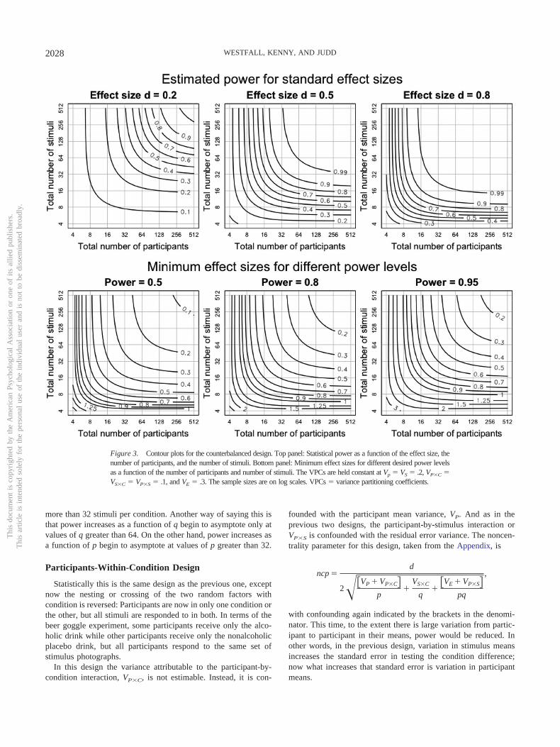
Participants-Within-Condition Design

Statistically this is the same design as the previous one, exceptnow the nesting or crossing of the two random factors withcondition is reversed: Participants are now in only one condition orthe other, but all stimuli are responded to in both. In terms of thebeer goggle experiment, some participants receive only the alco-holic drink while other participants receive only the nonalcoholicplacebo drink, but all participants respond to the same set ofstimulus photographs.

In this design the variance attributable to the participant-by-condition interaction, VP�C, is not estimable. Instead, it is con-

founded with the participant mean variance, VP. And as in theprevious two designs, the participant-by-stimulus interaction orVP�S is confounded with the residual error variance. The noncen-trality parameter for this design, taken from the Appendix, is

ncp �d

2��VP � VP�C�p

�VS�C

q�

�VE � VP�S�pq

,

with confounding again indicated by the brackets in the denomi-nator. This time, to the extent there is large variation from partic-ipant to participant in their means, power would be reduced. Inother words, in the previous design, variation in stimulus meansincreases the standard error in testing the condition difference;now what increases that standard error is variation in participantmeans.

Figure 3. Contour plots for the counterbalanced design. Top panel: Statistical power as a function of the effect size, thenumber of participants, and the number of stimuli. Bottom panel: Minimum effect sizes for different desired power levelsas a function of the number of participants and number of stimuli. The VPCs are held constant at Vp � VS � .2, VP�C �VS�C � VP�S � .1, and VE � .3. The sample sizes are on log scales. VPCs � variance partitioning coefficients.

Thi

sdo

cum

ent

isco

pyri

ghte

dby

the

Am

eric

anPs

ycho

logi

cal

Ass

ocia

tion

oron

eof

itsal

lied

publ

ishe

rs.

Thi

sar

ticle

isin

tend

edso

lely

for

the

pers

onal

use

ofth

ein

divi

dual

user

and

isno

tto

bedi

ssem

inat

edbr

oadl

y.


Under the assumptions that we have made, the power results forthis design, given in Figure 5, are the same as those given for theprevious design except they have been transposed so that nowpower is more dramatically affected by the number of participantsthan the number of stimuli. Even in the case of this design,however, it remains true that power of .80 is only achievable, givena moderate effect size, when the number of stimuli is greater than16, a number which is larger than that typically used.

Both-Within-Condition Design

The final design has each participant and also each stimulus inonly one of the two conditions, but within each condition all p/2participants judge all q/2 stimuli. From the beer goggle example,each participant consumes either alcohol or the placebo, and eachtarget is judged for attractiveness in only one of the two conditions.

In this design three different variance components are not esti-mable and are confounded with other components: the stimulus-by-condition component, VS�C, the participant-by-condition com-ponent, VP�C, and the participant-by-stimulus interactioncomponent, VP�S. The first of these is confounded with the stim-ulus intercept variance, the second with the participant interceptvariance, and the third with the residual error variance. From theAppendix, the noncentrality parameter for this design is

ncp �d

2 ��VP � VP�C�p

��VS � VS�C�

q�

2� VE � VP�S�pq

.

As a result, the standard error for testing the condition difference isinflated and power reduced to the extent that there exist both largeparticipant and large stimulus differences in their means.

Figure 4. Contour plots for the stimuli-within-condition design. Top panel: Statistical power as a function of the effectsize, the number of participants, and the number of stimuli. Bottom panel: Minimum effect sizes for different desired powerlevels as a function of the number of participants and number of stimuli. The VPCs are held constant at Vp � VS � .2,VP�C � VS�C � VP�S � .1, and VE � .3. The sample sizes are on log scales. VPCs � variance partitioning coefficients.

Thi

sdo

cum

ent

isco

pyri

ghte

dby

the

Am

eric

anPs

ycho

logi

cal

Ass

ocia

tion

oron

eof

itsal

lied

publ

ishe

rs.

Thi

sar

ticle

isin

tend

edso

lely

for

the

pers

onal

use

ofth

ein

divi

dual

user

and

isno

tto

bedi

ssem

inat

edbr

oadl

y.


The power results given in Figure 6 for this design are againsymmetric with respect to p and q under the assumptions we aremaking. And these power results are particularly poor, relative tothe other designs we have considered. With a moderate effect sizeand as many as 25 participants responding to 25 stimuli in eachcondition, power only equals .5. Even with unlimited numbers ofparticipants, power of .80 with a moderate effect size is achievableonly if the number of stimuli per condition is greater than roughly48.

Illustrative Example

To make our discussion of power analysis for these complexdesigns more concrete, here we work through an example for ahypothetical experiment. This example illustrates the process ofcoming up with some reasonable variance component and effect

size estimates given what we know about our study, using theonline power application to compute power and minimum num-bers of participants and/or stimuli, and investigating how theseanswers would change under different assumptions about the vari-ance components and effect size.

Consider a study where we are investigating the impact of acognitive load manipulation (e.g., memorizing short lists of inte-gers) on participants’ performance on a series of items from a taskthat depends on working memory capacity. The dependent variableis some continuous measure of each participant’s performance oneach item. We would like to employ a within-subject design whereeach participant responds to items both under cognitive load andnot under cognitive load, but we wish to avoid any potentialcarryover effects that might result from each participant respond-ing to each item twice (once under each load condition). Therefore,

Figure 5. Contour plots for the participants-within-condition design. Top panel: Statistical power as a functionof the effect size, the number of participants, and the number of stimuli. Bottom panel: Minimum effect sizesfor different desired power levels as a function of the number of participants and number of stimuli. The VPCsare held constant at Vp � VS � .2, VP�C � VS�C � VP�S � .1, and VE � .3. The sample sizes are on log scales.VPCs � variance partitioning coefficients.

Thi

sdo

cum

ent

isco

pyri

ghte

dby

the

Am

eric

anPs

ycho

logi

cal

Ass

ocia

tion

oron

eof

itsal

lied

publ

ishe

rs.

Thi

sar

ticle

isin

tend

edso

lely

for

the

pers

onal

use

ofth

ein

divi

dual

user

and

isno

tto

bedi

ssem

inat

edbr

oadl

y.


the items are divided into two lists, List A and List B, andparticipants are randomly assigned to either respond to the List Aitems under cognitive load and the List B items not under load, orto respond to the List B items under cognitive load and the List Aitems not under load. Thus, we employ the counterbalanced de-sign. We have two random factors, Participant and Item, and onefixed factor representing the overall difference in performancebetween the load and no-load conditions.

Suppose that we have developed a sample of 16 items (eight oneach list) for this working memory task. How many participants mustwe recruit to achieve statistical power of 0.8? We first examine someanswers to this question using the default set of VPCs that weproposed above (VE � .3;VP � VS � .2; VP�C � VS�C � VP�S �.1), and a medium effect size of d � 0.5. The online power application(located at http://jakewestfall.org/power/) has these VPCs as the de-fault. We specify the design as the counterbalanced design. Accord-ing to some recent recommendations (Simmons, Nelson, &

Simonsohn, 2011), a study should employ at least 20 partici-pants per between-subjects condition, so we start with thatvalue as the number of participants and enter 16 for the numberof stimuli (items). Pressing the Solve for X button, we find thatunder the VPC assumptions above, power would be .571. If wewant to know how many participants would be required toachieve statistical power of .80, we can enter the x symbol fornumber of participants, fill in .80 for power, and press Solve forX; the application informs us that we require 154 participants.

An examination of the power plots for this design (in Figure 3)makes clear that with only 16 items, the maximum power that canbe achieved, under the assumptions made, even with a very largenumber of participants, is only slightly above .8. These powerresults also make clear that if more power is to be achieved, moreitems are necessary. Accordingly, as a result of reading what hasbeen presented so far in this article, it is decided to increase thenumber of items to 30. Solving now for the number of participants

Figure 6. Contour plots for the both-within-condition design. Top panel: Statistical power as a function of the effect size,the number of participants, and the number of stimuli. Bottom panel: Minimum effect sizes for different desired power levelsas a function of the number of participants and number of stimuli. The VPCs are held constant at Vp � VS � .2, VP�C �VS�C � VP�S � .1, and VE � .3. The sample sizes are on log scales. VPCs � variance partitioning coefficients.

Thi

sdo

cum

ent

isco

pyri

ghte

dby

the

Am

eric

anPs

ycho

logi

cal

Ass

ocia

tion

oron

eof

itsal

lied

publ

ishe

rs.

Thi

sar

ticle

isin

tend

edso

lely

for

the

pers

onal

use

ofth

ein

divi

dual

user

and

isno

tto

bedi

ssem

inat

edbr

oadl

y.



to achieve power of .80, the application tells us that 27 participantsare needed. Clearly, increasing the number of stimuli makes alarge power difference.

In the absence of any information about the study we areplanning other than the possible sample sizes, the default set ofVPCs that we used above and a medium effect size togetherrepresent a reasonable set of assumptions that we might expect tobe approximately true for our study. But if we do know a littleabout the samples of participants and stimuli we are using and theeffect which we are studying, we can do better by tailoring whatwe expect the VPCs to be for the research being conducted. Forexample, suppose that we know that the items we developed forthe working memory task vary considerably in their average dif-ficulty (some items tend to yield low performance scores, whileothers tend to yield high performances scores); as a consequence,the more difficult ones might be affected more by the cognitiveload manipulation than the easier items. We also might know thatour participants are likely to be rather homogeneous in theiraverage working memory capacities and, we suspect, also in thedegree to which cognitive load would interfere in task perfor-mance. To reflect this knowledge, it seems reasonable to increasethe values of both VS and VS�C and to decrease the values of bothVP and VP�C. Accordingly, we decide to increase VS and VS�C to.25 and .15, respectively, and to decrease both VP and VP�C by thesame amounts (to .15 and .05, respectively). We leave the otherVPCs at their default values. These changes, tailored to our knowl-edge of the research domain, reveal that power of .80 is achievablewith 25 participants, again assuming that we have increased thenumber of items to 30.

In the process illustrated above, we started with some defaultvalues of the variance components and effect size, and then wemade adjustments to some of these default values based on sub-stantive knowledge that we had about the details of the particularstudy we would be running. However, we note that all of thesevalues, even the values we specifically adjusted, are ultimatelyeducated guesses about the true parameter values, and so theyshould be seen as implicitly containing a degree of uncertainty. Inacknowledgment of this, our recommendation is that researchersuse these educated guesses as a starting point in computing powerand sample size estimates for a range of plausible values of theparameters for the study at hand.

Optimal Design With Crossed Random Factors

On the basis of the above power analyses for our five designs,we can draw some general conclusions and formulate a variety ofrules of thumb concerning the optimal design of experimentswhere a sample of participants respond to a sample of stimuli. Inthis section, we discuss the maximum attainable power in anexperiment once the number of stimuli is fixed; when statisticalpower is best served by increasing the number of participants or byincreasing the number of stimuli; the relative efficiency of the fivedesigns; and finally the statistical merits of designs involvingmultiple blocks of stimuli as a way of dealing with the problem oftime-consuming stimulus presentation.

Maximum Attainable Power

One potentially surprising fact that we learn from our poweranalyses about the use of designs with crossed random factors is

that statistical power does not approach unity as the number ofparticipants approaches infinity, whenever there is variation due tostimuli. Instead, statistical power asymptotes at a maximum theo-retically attainable power value that depends on the effect size, thenumber of stimuli, and the variability of the stimuli. To see this inthe fully crossed design, consider what happens to the noncentral-ity parameter (ncpFC) as the number of participants (p) goes toinfinity:

limp¡

ncpFC � limp¡

d

2 �VP�C

p�

VS�C

q�

VE

2pq

�d �q

2 �VS�C

.

Notice here that when p goes to infinity, the terms in the denom-inator involving VE and VP�C disappear, but the numerator and theterm involving VS�C are both unchanged, so that in the limit thenoncentrality parameter converges to a finite (and possibly small)value. In Figure 7 we plot the maximum attainable power in thefully crossed design as a function of the effect size (d), the numberof stimuli (q) and the variance in the stimulus slopes (VS�C). Theseare contour plots just like the plots displayed earlier; the differenceis that instead of plotting the observed power for different combi-nations of parameters, they plot the upper bound for power atvarious combinations of parameters. The plots of maximum powerfor the other four designs all look nearly identical to those for thefully crossed design.

The primary lesson for experimenters following from the sta-tistical fact that maximum attainable power does not approachunity with increasing numbers of participants is that it is veryimportant to think carefully about the sample of stimuli in theexperiment before the data collection begins. Once data collectionbegins, the effect size and the number and properties of the stimulican no longer be changed, and thus the maximum power thatwould be attainable in the experiment has in essence already beendecided. All that then remains is to recruit a certain number ofparticipants, which determines how close to this maximum powerlevel the actual power ends up being. Experimenters may believethat they can compensate for a suboptimal sample of stimuli bysimply recruiting a larger number of participants, but in fact thedegree to which this sort of compensation can take place is quitelimited, a point which we discuss in more detail in the next section.The fact is that in many entirely realistic experimental situations,the maximum attainable power with an infinite number of partic-ipants can be quite low even for detecting true, large effects. Forexample, in an experiment employing the stimuli-within-conditiondesign, under the standard case VPCs described above, where thetrue effect size is large at d � 0.8, and where there are a total ofeight stimuli (four stimuli per condition)—a sample size which wesuspect many experimenters would consider perfectly adequate fora stimulus sample—the maximum attainable power is only about.41. However, if we just double the sample size of stimuli to a stillrelatively modest 16 (eight per condition), then the maximumpower to detect a large effect goes up to about .78.

Another implication of the maximum attainable power beingless than one is that in studies involving crossed random factors, adirect replication with high statistical power is often theoreticallyimpossible when the original study employed a relatively smallnumber of stimuli. Recently, researchers have stressed the impor-

Thi

sdo

cum

ent

isco

pyri

ghte

dby

the

Am

eric

anPs

ycho

logi

cal

Ass

ocia

tion

oron

eof

itsal

lied

publ

ishe

rs.

Thi

sar

ticle

isin

tend

edso

lely

for

the

pers

onal

use

ofth

ein

divi

dual

user

and

isno

tto

bedi

ssem

inat

edbr

oadl

y.


tance of conducting direct replications (Francis, 2012; Ioannidis,2012; Koole & Lakens, 2012; Nosek, Spies, & Motyl, 2012; OpenScience Collaboration, 2012) and also emphasized that replicationattempts should ideally have high statistical power, even when(perhaps especially when) the original study was underpowered(Brandt et al., 2014). Most typically, those who would replicate astudy with higher power than the original might employ the samestimuli but increase the number of participants to a level theyconsider adequate. However, to the extent that there is substantialstimulus variability, replications with high power may in fact notbe feasible using only the stimuli included in the original study.Sufficiently high power may be obtainable only by increasing thenumber of stimuli, as well as the numbers of participants.

We point out that a direct replication would virtually never usethe same participants as the original study. Instead, it wouldprobably just be assumed that the new participants were drawnfrom the same general population as the original participants. Whythen should we require the stimuli to be exactly the same as in theoriginal experiment, rather than just being drawn from the samepopulation? We strongly suggest that, when conducting a replica-tion of a study involving crossed random factors, it would bebeneficial for the researchers conducting the replication to aug-ment the stimulus set, drawing from the same population of stimulias in the original study, in order to ensure that statistical power isacceptably high. We discuss these issues in more detail in acompanion article (Westfall, Judd, & Kenny, 2014).

Increasing the Sample Sizes of ParticipantsVersus Stimuli

Not surprisingly, experiments with larger sample sizes of bothparticipants and stimuli always have greater power than experi-ments with smaller sample sizes. However, the question of

whether one can expect a greater benefit to statistical power byincreasing the sample size of participants or the sample size ofstimuli turns out to depend on several different aspects of theexperiment. Here we formulate two rules of thumb that researcherscan use to identify situations where it would be better to increasethe sample size of participants or of stimuli. Formally, these rulesof thumb are based on an analysis of the conditions under whichthe rate of change in the noncentrality parameter with respect tothe number of participants is greater than the rate of change in thenoncentrality parameter with respect to the number of stimuli (orvice versa). For example, to examine when it is better to increasethe sample size of stimuli rather than the sample size of partici-pants in the fully crossed design, we first set

�ncpFC

�q�

�ncpFC

�p.

With some work, we can simplify this inequality to obtain

pVE � 2p2VS � C � qVE � 2q2VP � C. (1)

We refer to this inequality in discussing the rules of thumb below.The first rule of thumb is that it is generally better to increase the

sample size of whichever random factor is contributing morerandom variation to the data, considering the nature of the responsevariable and the relevant properties of the participants and stimuli.Statistically speaking, this is because the primary statistical con-sequence of adding participants or adding stimuli is that thecorresponding participant or stimulus variance components, re-spectively, would become further diminished in their contributionto the denominator of the noncentrality parameter, and there is agreater advantage to diminishing the contribution of largervariance components compared to smaller variance compo-nents. An equivalent way of stating this is the following:

Figure 7. Contour plots of the maximum attainable power with an infinite number of participants in the fullycrossed design as a function of the effect size, number of stimuli (on a log scale), and the proportion of stimulusslope variance. The contour plots of maximum power for the other four designs all look nearly identical to theplots shown here.

Thi

sdo

cum

ent

isco

pyri

ghte

dby

the

Am

eric

anPs

ycho

logi

cal

Ass

ocia

tion

oron

eof

itsal

lied

publ

ishe

rs.

Thi

sar

ticle

isin

tend

edso

lely

for

the

pers

onal

use

ofth

ein

divi

dual

user

and

isno

tto

bedi

ssem

inat

edbr

oadl

y.


Different variance components contribute to the size of thenoncentrality parameter in different designs, and the extent towhich they contribute depends on the corresponding samplesize on which they are based, with larger sample sizes leadingto relatively less contribution. In terms of the example aboveconcerning the noncentrality parameter for the fully crosseddesign, we can see that if the two sample sizes are equal (i.e.,p � q) then Inequality 1 just reduces to VS�C VP�C

As an example of applying this rule of thumb, consider areaction time experiment where participants decide as quickly aspossible whether each of a list of written stimuli is a word or anonword. There is probably a great deal of variability betweenparticipants in both their mean reaction times and their differentialreaction times to words versus nonwords. However, assuming thestimuli are strictly controlled in terms of their number of letters,ease of pronunciation, and so on, there is probably comparativelylittle variability in the mean reaction times elicited by each stim-ulus. In this situation there would tend to be a greater powerbenefit to adding participants compared to adding stimuli. Alter-natively, consider an experiment where participants judge theattractiveness of a set of photographs of faces. It is probably thecase that some stimulus faces tend to elicit higher or lower attrac-tiveness ratings on average than do other stimulus faces, but thereis probably not as much individual difference variance in howattractive a participant considers stimulus faces on average(Hönekopp, 2006). In this situation there would tend to be a greaterbenefit of adding more stimuli compared to adding more partici-pants.

The second rule of thumb is that if one of the two sample sizesis considerably smaller than the other, there is generally a greaterpower benefit in increasing the smaller sample size compared tothe larger sample size—for two reasons. First and most obviously,the impact of either sample size has a diminishing-returns rela-tionship with statistical power, so that if one sample size is alreadylarge and the other is small, increases in the smaller sample sizewould have a greater impact on power. Second and more subtly,the two sample sizes together have a multiplicative effect onstatistical power, so that the rate at which increasing one of thesample sizes leads to an increase in power depends in part on themagnitude of the other sample size. To make this multiplicativerelationship clear in the case of the fully crossed design, consideragain Inequality 1. When the number of participants is largerelative to the number of stimuli this inequality is more likely to betrue (i.e., the left-hand side is more likely to exceed the right-handside), implying that there is greater incremental benefit to addingstimuli compared to adding participants. Likewise, when the num-ber of participants is small relative to the number of stimuli, thisinequality is more likely to be false, implying that there is greaterincremental benefit of adding participants. More generally, thisinequality shows that the relative rates of change of the noncen-trality parameter with respect to either of the sample sizes dependin part on the other sample size.

A somewhat insidious consequence of this multiplicative sam-ple size relationship is that the degree of trade-off that one canachieve with the sample sizes—that is, the degree to which aresearcher can compensate for having a small number of levels forone random factor by adding many more levels of the otherrandom factor—tends to be quite limited. Generally speaking, ifone of the sample sizes of the study is badly deficient, there is little

that one can realistically do with the size of the other sample torescue statistical power, both because of the multiplicative natureof the sample size relationship and because of the low maximumattainable power imposed by the small sample size. Unfortunately,we note that in many areas of the psychological literature, exper-iments with very small samples of stimuli (e.g., fewer than 10) arequite common. Our power results indicate that such studies oftenare badly underpowered even for detecting true large effects.

A final point to consider is the relative costs of increasing thesample sizes of the two random factors, relative to the powerbenefits accruing from those increases. In many circumstances, itmay be relatively more cost effective to increase the sample size ofstimuli than the sample size of participants. Once participants arerecruited for a study, increasing the time they spend in the lab byexposing them to additional stimuli is quite easy and therefore islikely more efficient from a logistical perspective than recruitingadditional participants. Again, because researchers have typicallynot treated stimuli as a random factor in analyses, the powerbenefits, perhaps accruing at relatively little cost, from using largersamples of stimuli have mostly been ignored. If the goal is toproduce replicable results that generalize across both participantand stimulus samples, then researchers clearly need to focus onboth random factors in their power considerations, taking intoaccount the power benefits of increasing both sample sizes relativeto the costs of doing so.

A Comparison of Crossed Designs

If researchers feel they have a good understanding of what kindof patterns of participant and stimulus variation to expect in astudy they are planning, and they also have some freedom to selectamong different design variations, the results of our power anal-yses can be used to help optimally select a design for studying thephenomenon of interest.

For a given total number of participants (p) and total number ofstimuli (q), the fully crossed design is the most efficient wheneverit is possible to run it. This is due to the facts that it provides thegreatest number of observations, and that it eliminates the partic-ipant intercept, the stimulus intercept, and the participant by stim-ulus interaction variance terms (VP, VS, and VP�S) from the de-nominator of the noncentrality parameter. In practice the twointercept variances, due to participants and due to stimuli, are oftenrelatively large.

The counterbalanced design, although not quite as powerful asthe fully crossed design for a given p and q, also tends to berelatively powerful. Although it yields half as many total obser-vations as the fully crossed design for a given total number ofparticipants and total number of stimuli, it shares the advantage ofeliminating the participant intercept and stimulus intercept vari-ance terms (VS and VP) from the denominator of the noncentralityparameter. It does not, however, eliminate the participant by stim-ulus interaction component (VP�S), which is confounded witherror in this design.

Note that the fully crossed design requires participants to maketwice as many responses for the same number of stimuli as thecounterbalanced design. For a fairer comparison of the two de-signs, we should allow the counterbalanced design to have twicethe number of stimuli as the fully crossed design. If an experi-menter only has enough time in an experimental session to elicit,

Thi

sdo

cum

ent

isco

pyri

ghte

dby

the

Am

eric

anPs

ycho

logi

cal

Ass

ocia

tion

oron

eof

itsal

lied

publ

ishe

rs.

Thi

sar

ticle

isin

tend

edso

lely

for

the

pers

onal

use

ofth

ein

divi

dual

user

and

isno

tto

bedi

ssem

inat

edbr

oadl

y.


say, 100 responses from each participant, then the counterbalanceddesign would allow the employment of a sample of 100 stimuli,while the fully crossed design would only support a sample of 50stimuli. It therefore seems that a more reasonable way to comparethe two designs might be not to hold constant the number ofstimuli but to hold constant the number of responses made by eachparticipant. How do the fully crossed and counterbalanced designsstack up when compared in this way?

To compare the efficiency of the counterbalanced design and thefully crossed design with the number of responses per participantheld constant, we first set the noncentrality parameter for thecounterbalanced design (ncpCB) greater than the noncentrality pa-rameter for the fully crossed design (ncpFC):

ncpCB � ncpFC.

Now we substitute in the definitions of these centrality parameters,but set the number of stimuli to 2q in the counterbalanced designand to q in the fully crossed design, which equates the two designsin the total number of responses made per participant:

d

2 �VP�C

p�

VS�C

2q�

�VE � VP�S�2pq

�d

2 �VP�C

p�

VS�C

q�

VE

2pq

.

Finally, we simplify this inequality to obtain

p �VP�S

VS�C.

In words, the counterbalanced design has greater power than thefully crossed design when the ratio of participant-by-stimulusinteraction variance (VP�S) to stimulus slope variance (VS�C) isless than the number of participants (p). We note that this conditionis almost always true in any realistic data set. For example, if anexperiment involves 50 participants, then we would need to havemore than 50 times as much participant-by-stimulus variance asstimulus slope variance for this condition to fail. While there maybe many contexts in which we do expect VP�S to exceed VS�C,very rarely would we expect it to do so by a factor of more than 50.Thus, if the number of responses per participant is held constantrather than the number of stimuli, then the counterbalanced designis actually more efficient in most cases than the fully crosseddesign. The reason for this advantage is that the counterbalanceddesign can employ twice as many stimuli using the same numberof total responses from each participant, leading to a doubling ofone of the sample sizes of the study. It therefore seems that thechoice of whether to use the fully crossed design or the counter-balanced design comes to down to whether the main constraint inthe size of the experiment comes from the maximum number ofresponses that one can collect from each participant, or from thenumber of stimuli available to respond to. If one has only a smallnumber of stimuli but is able to elicit more responses from eachparticipant, then the fully crossed design is preferable. If one hasa large stimulus pool but is limited in the number of responses that

can be collected from each participant, then the counterbalanceddesign is preferable.

Moving now to the stimuli-within-condition and participants-within-condition designs, the relative efficiency of these two de-signs depends totally on the relative magnitudes of the participantand stimulus variance components and on the two sample sizes. Ifwe set the noncentrality parameter for the Stimuli-within-conditiondesign greater than the noncentrality parameter for theparticipants-within-condition design, we find that the stimuli-within-condition design is more powerful than the participants-within-condition design when

VP

p�

VS

q.

In other words, if there is a great deal of variance in the meanresponses of participants (VP is high) or if the number of partici-pants (p) is small, then the stimuli-within-condition design tends tobe relatively more efficient. But if it is the stimuli that haverelatively more variance in their mean responses elicited (VS ishigh), or if the number of stimuli (q) is small, then the participants-within-condition design tends to be more efficient, all other thingsbeing equal.

Finally, the both-within-condition design generally has the low-est power of the five designs considered here. This design yieldsthe lowest number of total observations for a given total number ofparticipants and total number of stimuli, and the denominator ofthe noncentrality parameter in this design implicitly contains allpossible sources of variation, whereas for the other four designs,one or more of the sources of variance are absent.

Dealing With Time-Consuming Stimulus Presentation:Stimuli-Within-Block Designs and Nested Designs

One of the major practical lessons in this article is that to ensureadequate statistical power, stimulus samples usually need to be atleast moderately sized; in any case, larger than is very often seenin many areas of experimental psychology. However, there aremany research paradigms in which it is infeasible to have eachparticipant respond to more than a handful of stimuli. For example,if it is determined that a sample size of 60 stimuli is needed forstatistical power reasons, but the stimuli are 5-minute film clips orsongs that participants must view or listen to in their entiretybefore making each response, then the counterbalanced design forexample would require each participant to spend over 5 hoursviewing and responding to stimuli, which is likely impractical dueto concerns of participant fatigue, time constraints on the durationof individual experimental sessions, and other reasons.

A solution to this dilemma is to use what we call a stimuli-within-block design (see Table 3). These are conceptually relatedto matrix sampling designs from survey research, an example of aplanned missing data design (Graham, Taylor, Olchowski, & Cum-sille, 2006; Shoemaker, 1973). In a stimuli-within-block design,the full stimulus sample is divided into a smaller number ofcomparable lists or blocks, and each participant is randomly as-signed to receive only one of these blocks. In the previous exampleof an experiment involving a sample of 60 film clips or songs,these stimuli could be divided into, say, 10 blocks of six stimulieach. If each participant responds to only one of these blocks, then

Thi

sdo

cum

ent

isco

pyri

ghte

dby

the

Am

eric

anPs

ycho

logi

cal

Ass

ocia

tion

oron

eof

itsal

lied

publ

ishe

rs.

Thi

sar

ticle

isin

tend

edso

lely

for

the

pers

onal

use

ofth

ein

divi

dual

user

and

isno

tto

bedi

ssem

inat

edbr

oadl

y.


each experimental session could take around 30 minutes. Thepromise of stimuli-within-block designs is that as long as theresearcher is willing to spend some extra time assembling a largerstimulus sample, the study can enjoy the greater statistical powerassociated with larger stimulus samples while still avoiding plac-ing heavy time demands on the participants.

To give a sense of the relative statistical efficiency of stimuli-within-block designs compared to the more commonly usedcrossed designs, we conducted a simulation examining the exper-imental design mentioned above, where 60 participants each re-spond to six stimuli, three in each condition. In this simulation weheld constant the number of participants and the number of re-sponses made by each participant, but varied the number of uniquestimulus blocks from one to 60, so that the total number of stimuliranged from six to 360 across the simulated experiments, with theassumption that stimuli are randomly assigned to blocks.5 Notethat when there is a single stimulus block, every participant re-sponds to the same set of stimuli, and this particular stimuli-within-block design reduces to the crossed stimuli-within-condition design. At the other extreme, when the number ofstimulus blocks equals the number of participants, then everyparticipant responds to their own unique set of stimuli in what iscommonly known as a nested design (Raudenbush, 1997; Rauden-bush & Liu, 2000; Snijders, 2001; Snijders & Bosker, 1993). Therelative statistical efficiency of these three types of designs, de-fined as the relative widths of the standard errors of the conditiondifference, is illustrated in Figure 8, which is based on the standardcase variance components described earlier. In this example, in-creasing the number of stimulus blocks from one to 10 (so that thetotal number of stimuli increases from six to 60) increases statis-tical efficiency by a factor of about 2.3.

The major take-away point here is that even in experimentalparadigms that involve time-consuming stimulus presentation, it isstill possible to employ a reasonably large sample of stimuli byusing a stimuli-within-block design; treating stimuli as randomneed not necessarily lead to a substantial decrease in statisticalpower even in these paradigms.

Sometimes it is even possible to assign a unique set of stimuli toevery participant, leading to a nested design. From a logistical

perspective, running an experiment with a fully nested designmight be difficult, as it not only requires a very large number ofstimuli but also requires that the experiment be conducted in sucha way that no participant ever receives a stimulus that has beenresponded to by another participant. However, in those situationswhere it is feasible, there are potentially large statistical powerbenefits to employing this kind of nested design compared to thecrossed designs that we have focused on in this article. Notably, inaddition to the statistical power advantage illustrated in Figure 8,in fully nested designs statistical power does approach unity as thenumber of participants goes to infinity, unlike in the crossed andstimuli-within-block designs.

Concluding Remarks

For all too many years, until the groundbreaking work of JacobCohen and others, experimental psychologists paid little attentionto issues of statistical power. Fortunately, that situation has begunto change. There are now discussions about how experimentsshould be optimally designed to maximize statistical power, al-though most of these discussions focus simply on making sure thatadequate numbers of participants are recruited (for exceptions seeBaguley, 2004; McClelland, 1997, 2000).

Hardly ever, however, in this increasing discussion of optimaldesign and statistical power does one hear mention of the samplingof stimuli to which participants are exposed. We all have rules ofthumb in particular contexts about how stimuli should be con-structed, about pretesting that ought to be done to ensure thatstimuli represent what we hope they do, and about the approximatenumbers of stimuli that should be employed. But by and largethese rules of thumb are not informed by considerations of statis-tical power. Our goal in writing this article is to begin to change

5 We note that this is not the only reasonable way that stimuli could bedivided into blocks. For example, blocks could be deliberately constructedso that the variation across blocks in their overall mean responses or theircondition differences was as small as possible, and these decisions wouldhave power consequences. However, we consider these issues to be outsidethe scope of our limited discussion here, and so for simplicity we justassume that stimuli are randomly assigned to blocks.

Table 3Schematic for a Particular Stimuli-Within-Block Design That Is an Extension of the Stimuli-Within-Condition Design

Participants

Stimuli

1 2 3 4 5 6 7 8 9 10 11 12 13 14 15 16

1 A A B B — — — — — — — — — — — —2 A A B B — — — — — — — — — — — —3 A A B B — — — — — — — — — — — —4 — — — — A A B B — — — — — — — —5 — — — — A A B B — — — — — — — —6 — — — — A A B B — — — — — — — —7 — — — — — — — — A A B B — — — —8 — — — — — — — — A A B B — — — —9 — — — — — — — — A A B B — — — —

10 — — — — — — — — — — — — A A B B11 — — — — — — — — — — — — A A B B12 — — — — — — — — — — — — A A B B

Note. Each participant is randomly assigned to respond to one of four stimulus blocks, each block containing four stimuli. A means that this participantresponds to this stimulus only under Condition A; B means that this participant responds to this stimulus only under Condition B. A dash means that thisparticipant never responds to this stimulus.

Thi

sdo

cum

ent

isco

pyri

ghte

dby

the

Am

eric

anPs

ycho

logi

cal

Ass

ocia

tion

oron

eof

itsal

lied

publ

ishe

rs.

Thi

sar

ticle

isin

tend

edso

lely

for

the

pers

onal

use

ofth

ein

divi

dual

user

and

isno

tto

bedi

ssem

inat

edbr

oadl

y.


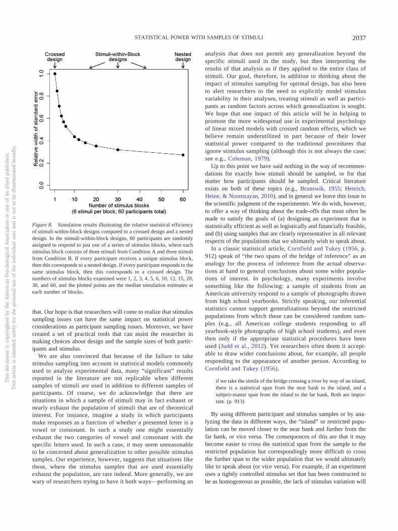
that. Our hope is that researchers will come to realize that stimulussampling issues can have the same impact on statistical powerconsiderations as participant sampling issues. Moreover, we havecreated a set of practical tools that can assist the researcher inmaking choices about design and the sample sizes of both partic-ipants and stimulus.

We are also convinced that because of the failure to takestimulus sampling into account in statistical models commonlyused to analyze experimental data, many “significant” resultsreported in the literature are not replicable when differentsamples of stimuli are used in addition to different samples ofparticipants. Of course, we do acknowledge that there aresituations in which a sample of stimuli may in fact exhaust ornearly exhaust the population of stimuli that are of theoreticalinterest. For instance, imagine a study in which participantsmake responses as a function of whether a presented letter is avowel or consonant. In such a study one might essentiallyexhaust the two categories of vowel and consonant with thespecific letters used. In such a case, it may seem unreasonableto be concerned about generalization to other possible stimulussamples. Our experience, however, suggests that situations likethese, where the stimulus samples that are used essentiallyexhaust the population, are rare indeed. More generally, we arewary of researchers trying to have it both ways—performing an

analysis that does not permit any generalization beyond thespecific stimuli used in the study, but then interpreting theresults of that analysis as if they applied to the entire class ofstimuli. Our goal, therefore, in addition to thinking about theimpact of stimulus sampling for optimal design, has also beento alert researchers to the need to explicitly model stimulusvariability in their analyses, treating stimuli as well as partici-pants as random factors across which generalization is sought.We hope that one impact of this article will be in helping topromote the more widespread use in experimental psychologyof linear mixed models with crossed random effects, which webelieve remain underutilized in part because of their lowerstatistical power compared to the traditional procedures thatignore stimulus sampling (although this is not always the case;see e.g., Coleman, 1979).

Up to this point we have said nothing in the way of recommen-dations for exactly how stimuli should be sampled, or for thatmatter how participants should be sampled. Critical literatureexists on both of these topics (e.g., Brunswik, 1955; Henrich,Heine, & Norenzayan, 2010), and in general we leave this issue tothe scientific judgment of the experimenter. We do wish, however,to offer a way of thinking about the trade-offs that must often bemade to satisfy the goals of (a) designing an experiment that isstatistically efficient as well as logistically and financially feasible,and (b) using samples that are clearly representative in all relevantrespects of the populations that we ultimately wish to speak about.

In a classic statistical article, Cornfield and Tukey (1956, p.912) speak of “the two spans of the bridge of inference” as ananalogy for the process of inference from the actual observa-tions at hand to general conclusions about some wider popula-tions of interest. In psychology, many experiments involvesomething like the following: a sample of students from anAmerican university respond to a sample of photographs drawnfrom high school yearbooks. Strictly speaking, our inferentialstatistics cannot support generalizations beyond the restrictedpopulations from which these can be considered random sam-ples (e.g., all American college students responding to allyearbook-style photographs of high school students), and eventhen only if the appropriate statistical procedures have beenused (Judd et al., 2012). Yet researchers often deem it accept-able to draw wider conclusions about, for example, all peopleresponding to the appearance of another person. According toCornfield and Tukey (1956),

if we take the simile of the bridge crossing a river by way of an island,there is a statistical span from the near bank to the island, and asubject-matter span from the island to the far bank. Both are impor-tant. (p. 913)

By using different participant and stimulus samples or by ana-lyzing the data in different ways, the “island” or restricted popu-lation can be moved closer to the near bank and further from thefar bank, or vice versa. The consequences of this are that it maybecome easier to cross the statistical span from the sample to therestricted population but correspondingly more difficult to crossthe further span to the wider population that we would ultimatelylike to speak about (or vice versa). For example, if an experimentuses a tightly controlled stimulus set that has been constructed tobe as homogeneous as possible, the lack of stimulus variation will

Figure 8. Simulation results illustrating the relative statistical efficiencyof stimuli-within-block designs compared to a crossed design and a nesteddesign. In the stimuli-within-block designs, 60 participants are randomlyassigned to respond to just one of a series of stimulus blocks, where eachstimulus block consists of three stimuli from Condition A and three stimulifrom Condition B. If every participant receives a unique stimulus block,then this corresponds to a nested design. If every participant responds to thesame stimulus block, then this corresponds to a crossed design. Thenumbers of stimulus blocks examined were 1, 2, 3, 4, 5, 6, 10, 12, 15, 20,30, and 60, and the plotted points are the median simulation estimates ateach number of blocks.

Thi

sdo

cum

ent

isco

pyri

ghte

dby

the

Am

eric

anPs

ycho

logi

cal

Ass

ocia

tion

oron

eof

itsal

lied

publ

ishe

rs.

Thi

sar

ticle

isin

tend

edso

lely

for

the

pers

onal

use

ofth

ein

divi

dual

user

and

isno

tto

bedi

ssem

inat

edbr

oadl

y.


often make it especially easy to obtain very precise estimates ofexperimental effects in this narrow population of stimuli, but it willoften be less obvious that these precisely estimated effects arerepresentative of those found in more natural settings. As anotherexample, if one analyzes the data using a statistical model thatincorporates uncertainty in the parameter estimates due to randomstimulus variation (Judd et al., 2012), it will often be more difficultto obtain precise estimates of effects—a cost that we hope thelessons of this article will help to mitigate—but upon crossing thislengthened statistical span, it will then be easier to generalize theresults to further, more interesting populations.

Though much has been covered here, the scope of our dis-cussion is limited in several key ways. We have confinedourselves to only a few designs, involving only two levels ofone fixed factor, when in practice many more complicateddesigns are used. In theory the present work could be extendedto higher designs involving multiple categorical fixed factors,although these extensions are not without some complications,such as a larger number of random slopes to consider; we leaveit to future research to work out these important issues. We havealso confined ourselves to outcome measures that are nicelybehaved, so that the underlying distributions of random effectsin our models could be assumed to be normal. And we haveconfined ourselves to considering issues of optimal design andpower only in relatively abstract contexts, divorced from therealities and constraints of any particular research paradigm andendeavor. We recognize that issues of design and power arenecessarily more complicated than the relatively simple frame-work we have used here.

That said, we would be very gratified indeed if this articlebegins the discussion of how stimuli ought to be sampled inexperimental research to achieve desirable levels of statisticalpower. We are convinced that the failure to recognize the randomvariation in data that results from stimulus variability has led us togive confidence to results that might routinely be nonreplicableexcept with the exact same stimuli. Moreover, we are convincedthat the failure to appreciate the role of stimulus variability seri-ously affects the statistical power of much of our research. Hope-fully, the tools we have provided can help us as a discipline tobegin to overcome these problems.

References

Asendorpf, J. B., Conner, M., De Fruyt, F., De Houwer, J., Denissen,J. J. A., Fiedler, K., . . . Wicherts, J. M. (2013). Recommendations forincreasing replicability in psychology. European Journal of Personality,27, 108–119. doi:10.1002/per.1919

Baayen, R. H., Davidson, D. J., & Bates, D. M. (2008). Mixed-effectsmodeling with crossed random effects for subjects and items. Journal ofMemory and Language, 59, 390–412. doi:10.1016/j.jml.2007.12.005

Baguley, T. (2004). Understanding statistical power in the context ofapplied research. Applied Ergonomics, 35, 73–80. doi:10.1016/j.apergo.2004.01.002

Bakker, M., van Dijk, A., & Wicherts, J. M. (2012). The rules of the gamecalled psychological science. Perspectives on Psychological Science, 7,543–554. doi:10.1177/1745691612459060

Barr, D. J., Levy, R., Scheepers, C., & Tily, H. J. (2013). Random effectsstructure for confirmatory hypothesis testing: Keep it maximal. Journalof Memory and Language, 68, 255–278. doi:10.1016/j.jml.2012.11.001

Brandt, M. J., IJzerman, H., Dijksterhuis, A., Farach, F. J., Geller, J.,Giner-Sorolla, R., . . . van ’t Veer, A. (2014). The replication recipe:

What makes for a convincing replication? Journal of ExperimentalSocial Psychology, 50, 217–224. doi:10.1016/j.jesp.2013.10.005

Brunswik, E. (1955). Representative design and probabilistic theory in afunctional psychology. Psychological Review, 62, 193–217. doi:10.1037/h0047470

Button, K. S., Ioannidis, J. P. A., Mokrysz, C., Nosek, B. A., Flint, J.,Robinson, E. S. J., & Munafò, M. R. (2013). Power failure: Why smallsample size undermines the reliability of neuroscience. Nature ReviewsNeuroscience, 14, 365–376. doi:10.1038/nrn3475

Clark, H. H. (1973). The language-as-fixed-effect fallacy: A critique oflanguage statistics in psychological research. Journal of Verbal Learn-ing and Verbal Behavior, 12, 335–359. doi:10.1016/S0022-5371(73)80014-3

Cohen, J. (1988). Statistical power analysis for the behavioral sciences.Hillsdale, NJ: Erlbaum.

Coleman, B. E. (1964). Generalizing to a language population. Psycholog-ical Reports, 14, 219–226. doi:10.2466/pr0.1964.14.1.219

Coleman, E. B. (1979). Generalization effects vs random effects: Is �TL2a source of Type 1 or Type 2 error? Journal of Verbal Learning &Verbal Behavior, 18, 243–256. doi:10.1016/S0022-5371(79)90145-2

Cornfield, J., & Tukey, J. W. (1956). Average values of mean squares infactorials. Annals of Mathematical Statistics, 27, 907–949. doi:10.1214/aoms/1177728067

Dixon, W. J., & Massey, F. J. (1957). Introduction to statistical analysis.New York, NY: McGraw-Hill.

Francis, G. (2012). Publication bias and the failure of replication inexperimental psychology. Psychonomic Bulletin & Review, 19, 975–991. doi:10.3758/s13423-012-0322-y

Goldstein, H., Browne, W., & Rasbash, J. (2002). Partitioning variation inmultilevel models. Understanding Statistics, 1, 223–231. doi:10.1207/S15328031US0104_02

Graham, J. W., Taylor, B. J., Olchowski, A. E., & Cumsille, P. E. (2006).Planned missing data designs in psychological research. PsychologicalMethods, 11, 323–343. doi:10.1037/1082-989X.11.4.323

Henrich, J., Heine, S. J., & Norenzayan, A. (2010). The weirdest people inthe world? Behavioral and Brain Sciences, 33, 61–83. doi:10.1017/S0140525X0999152X

Hönekopp, J. (2006). Once more: Is beauty in the eye of the beholder?Relative contributions of private and shared taste to judgments of facialattractiveness. Journal of Experimental Psychology: Human Perceptionand Performance, 32, 199–209. doi:10.1037/0096-1523.32.2.199

Ioannidis, J. P. A. (2008). Why most discovered true associations are inflated.Epidemiology, 19, 640–648. doi:10.1097/EDE.0b013e31818131e7

Ioannidis, J. P. A. (2012). Why science is not necessarily self-correcting.Perspectives on Psychological Science, 7, 645– 654. doi:10.1177/1745691612464056

Judd, C. M., Westfall, J., & Kenny, D. A. (2012). Treating stimuli as arandom factor in social psychology: A new and comprehensive solutionto a pervasive but largely ignored problem. Journal of Personality andSocial Psychology, 103, 54–69. doi:10.1037/a0028347

Kenny, D. A. (1994). Interpersonal perception: A social relations analysis.New York, NY: Guilford Press.

Koole, S. L., & Lakens, D. (2012). Rewarding replications: A sure andsimple way to improve psychological science. Perspectives on Psycho-logical Science, 7, 608–614. doi:10.1177/1745691612462586

Li, X., Sudarsanam, N., & Frey, D. D. (2006). Regularities in data fromfactorial experiments. Complexity, 11, 32–45. doi:10.1002/cplx.20123

McClelland, G. H. (1997). Optimal design in psychological research.Psychological Methods, 2, 3–19. doi:10.1037/1082-989X.2.1.3

McClelland, G. H. (2000). Increasing statistical power without increasingsample size. American Psychologist, 55, 963–964. doi:10.1037/0003-066X.55.8.963

Montgomery, D. C. (2013). Design and analysis of experiments (Vol. 8).New York, NY: Wiley.

Thi

sdo

cum

ent

isco

pyri

ghte

dby

the

Am

eric

anPs

ycho

logi

cal

Ass

ocia

tion

oron

eof

itsal

lied

publ

ishe

rs.

Thi

sar

ticle

isin

tend

edso

lely

for

the

pers

onal

use

ofth

ein

divi

dual

user

and

isno

tto

bedi

ssem

inat

edbr

oadl

y.


http://dx.doi.org/10.1002/per.1919

http://dx.doi.org/10.1016/j.jml.2007.12.005

http://dx.doi.org/10.1016/j.apergo.2004.01.002

http://dx.doi.org/10.1016/j.apergo.2004.01.002

http://dx.doi.org/10.1177/1745691612459060

http://dx.doi.org/10.1016/j.jml.2012.11.001

http://dx.doi.org/10.1016/j.jesp.2013.10.005

http://dx.doi.org/10.1037/h0047470

http://dx.doi.org/10.1037/h0047470

http://dx.doi.org/10.1038/nrn3475

http://dx.doi.org/10.1016/S0022-5371%2873%2980014-3

http://dx.doi.org/10.1016/S0022-5371%2873%2980014-3

http://dx.doi.org/10.2466/pr0.1964.14.1.219

http://dx.doi.org/10.1016/S0022-5371%2879%2990145-2

http://dx.doi.org/10.1214/aoms/1177728067

http://dx.doi.org/10.1214/aoms/1177728067

http://dx.doi.org/10.3758/s13423-012-0322-y

http://dx.doi.org/10.1207/S15328031US0104_02

http://dx.doi.org/10.1207/S15328031US0104_02

http://dx.doi.org/10.1037/1082-989X.11.4.323

http://dx.doi.org/10.1017/S0140525X0999152X

http://dx.doi.org/10.1017/S0140525X0999152X

http://dx.doi.org/10.1037/0096-1523.32.2.199

http://dx.doi.org/10.1097/EDE.0b013e31818131e7

http://dx.doi.org/10.1177/1745691612464056

http://dx.doi.org/10.1177/1745691612464056

http://dx.doi.org/10.1037/a0028347

http://dx.doi.org/10.1177/1745691612462586

http://dx.doi.org/10.1002/cplx.20123

http://dx.doi.org/10.1037/1082-989X.2.1.3

http://dx.doi.org/10.1037/0003-066X.55.8.963

http://dx.doi.org/10.1037/0003-066X.55.8.963

Nosek, B. A., Spies, J. R., & Motyl, M. (2012). Scientific Utopia II.Restructuring incentives and practices to promote truth over publishabil-ity. Perspectives on Psychological Science, 7, 615–631. doi:10.1177/1745691612459058

Open Science Collaboration. (2012). An open, large-scale, collaborative effortto estimate the reproducibility of psychological science. Perspectives onPsychological Science, 7, 657–660. doi:10.1177/1745691612462588

Raudenbush, S. W. (1997). Statistical analysis and optimal design forcluster randomized trials. Psychological Methods, 2, 173–185. doi:10.1037/1082-989X.2.2.173

Raudenbush, S. W., & Liu, X. (2000). Statistical power and optimal designfor multisite randomized trials. Psychological Methods, 5, 199–213.doi:10.1037/1082-989X.5.2.199

Rosenthal, R., & Rubin, D. B. (1982). Comparing effect sizes of indepen-dent studies. Psychological Bulletin, 92, 500–504. doi:10.1037/0033-2909.92.2.500

Santa, J. L., Miller, J. J., & Shaw, M. L. (1979). Using quasi F to preventalpha inflation due to stimulus variation. Psychological Bulletin, 86,37–46. doi:10.1037/0033-2909.86.1.37

Schimmack, U. (2012). The ironic effect of significant results on thecredibility of multiple-study articles. Psychological Methods, 17, 551–566. doi:10.1037/a0029487

Shoemaker, D. M. (1973). Principles and procedures of multiple matrixsampling. Cambridge, MA: Ballinger.

Simmons, J. P., Nelson, L. D., & Simonsohn, U. (2011). False-positivepsychology: Undisclosed flexibility in data collection and analysis al-lows presenting anything as significant. Psychological Science, 22,1359–1366. doi:10.1177/0956797611417632

Snijders, T. A. B. (2001). Sampling. In H. Goldstein & A. Leyland (Eds.),Multilevel modeling of health statistics (pp. 159–174). New York, NY:Wiley.

Snijders, T. A. B., & Bosker, R. J. (1993). Standard errors and sample sizesfor two-level research. Journal of Educational Statistics, 18, 237–259.doi:10.3102/10769986018003237

Wells, G. L., & Windschitl, P. D. (1999). Stimulus sampling and socialpsychological experimentation. Personality and Social Psychology Bul-letin, 25, 1115–1125. doi:10.1177/01461672992512005

Westfall, J., Judd, C. M., & Kenny, D. A. (2014). Replicating studies inwhich samples of participants respond to samples of stimuli.

Winer, B. J. (1971). Statistical principles in experimental design. NewYork, NY: McGraw–Hill.

Wu, C. J., & Hamada, M. S. (2000). Experiments: Planning, analysis, andoptimization. New York, NY: Wiley.

Appendix

Statistical Details of Power Analysis

In this Appendix, we provide the statistical details underlying the power results in the main article. We consider only experiments whereparticipants respond to each stimulus no more than once per condition; in other words, we assume only a single replication at the lowestlevel of observation. Within this constraint, we consider all potential sources of random variation. Consequently, the fully specified mixedmodel for the response of the ith participant to the jth stimulus in the kth condition is

yijk � �0 � �1ck � �iP � �i


S�Cck � �ijP�S � εijk,

var ��iP� � �P

2 , var � �iP�C� � �P�C

2 , var ��jS� � �S

2,

var ��jS�C� � �S�C

2 , var ��ijP�S� � �P�S

2 , var �εijk� � �E2 .

In this model, �0 and �1ck represent the fixed effects and capture, respectively, the overall mean response and the condition differencein responses. We assume the values of ck are contrast or deviation coded so that c1 � c2 � 0 and c1

2 � c22 � c2. For example, the values

of ck might be �1, �1, or �1/2, �1/2. Importantly, the values of ck are assumed not to be dummy or treatment coded (e.g., c1 � 0, c2 �1), as this totally alters the meanings of the variance components (see also Barr, Levy, Scheepers, & Tily, 2013, footnote 2). There arealso two covariance terms—that between the participant intercepts and slopes, �P, P�C, and between the stimulus intercepts and slopes,�S, S�C—but these can be omitted as unnecessary for reasons that are explained later in this Appendix. Finally, in what follows we assumethat the experiments are balanced and have no missing data.

We follow Cohen’s (1988) general approach to power analysis. In this approach, power estimation can be viewed as a three-stageprocess. We first select a suitable measure of effect size and define its value. In this article we rely on the standardized mean differencebetween conditions, Cohen’s d. Next we rescale the effect size by an adjustment factor, sometimes called the design effect (Snijders, 2001),that depends on the particular experimental design chosen, yielding what Cohen (1988, p. 13) refers to as the operative effect size. Finally,we scale the operative effect size by a term that includes information about the number of observations in the study. This final quantityis known as the noncentrality parameter (ncp), and with it and the degrees of freedom (df) we can compute power. This last step is oftenhidden in power analyses, but it shows how the operative effect size is adjusted by the sample sizes to compute a power value. To go fromthe noncentrality parameter to a power estimate, Cohen (1988, p. 544) relied on an approximation put forward by Dixon and Massey(1957). We have adopted a more exact approach that directly computes areas under the appropriate noncentral t distribution.

(Appendix continues)

Thi

sdo

cum

ent

isco

pyri

ghte

dby

the

Am

eric

anPs

ycho

logi

cal

Ass

ocia

tion

oron

eof

itsal

lied

publ

ishe

rs.

Thi

sar

ticle

isin

tend

edso

lely

for

the

pers

onal

use

ofth

ein

divi

dual

user

and

isno

tto

bedi

ssem

inat

edbr

oadl

y.


http://dx.doi.org/10.1177/1745691612459058

http://dx.doi.org/10.1177/1745691612459058

http://dx.doi.org/10.1177/1745691612462588

http://dx.doi.org/10.1037/1082-989X.2.2.173

http://dx.doi.org/10.1037/1082-989X.2.2.173

http://dx.doi.org/10.1037/1082-989X.5.2.199

http://dx.doi.org/10.1037/0033-2909.92.2.500

http://dx.doi.org/10.1037/0033-2909.92.2.500

http://dx.doi.org/10.1037/0033-2909.86.1.37

http://dx.doi.org/10.1037/a0029487

http://dx.doi.org/10.1177/0956797611417632

http://dx.doi.org/10.3102/10769986018003237

http://dx.doi.org/10.1177/01461672992512005

Effect Size and Variance Partitioning Coefficients

With stimuli as well as participants as random factors in a design, the simple effect size measure d must be defined more generally toreflect all of these possible variation sources. That is, instead of defining the effect size in terms of the expected mean difference dividedby the standard deviation across participants within condition, we define the effect size as the expected mean difference divided by thestandard deviation across participants and stimuli within condition (i.e., the square root of the expected variance of the individualobservations within a condition, pooled across both conditions). Let var(y1) and var(y2) be the variances of the response at the two levelsof the contrast-coded predictors. Then the pooled variance is

var(y1)

2�

var(y2)

2�

��P2 � c2�P�C

2 � �S2 � c2�S�C

2 � �P�S2 � �E

2 � 2c1�P,P�C � 2c1�S,S�C�2

��P

2 � c2�P�C2 � �S

2 � c2�S�C2 � �P�S

2 � �E2 � 2c2�P,P�C � 2c2�S,S�C�

2

� �P2 � c2�P�C

2 � �S2 � c2�S�C

2 � �P�S2 � �E

2 � (�P,P�C � �S,S�C) (c1 � c2)

� �P2 � c2�P�C

2 � �S2 � c2�S�C

2 � �P�S2 � �E

2 .

Notice that the covariance terms drop out, using the fact that c1 � c2 � 0 (i.e., that the predictor is contrast coded). This makes the effectsize based on the pooled variance

d ��1 �2

��

�1 �2

��P2 � c2�P�C

2 � �S2 � c2�S�C

2 � �P�S2 � �E

2.

Technically, the denominator of this effect size (i.e., the pooled variance) is a function of the predictor c, so that the variance of y ispotentially different at different levels of the predictor, a fact pointed out by Goldstein et al. (2002). However, we note that under ourassumption that the predictor is contrast coded, this denominator is identical at both levels of c.

We standardize the variance components by expressing them as variance partitioning coefficients (VPCs; Goldstein et al., 2002),specifically, as proportions of the total pooled variance. This leads to the following definitions of all standardized and unstandardizedquantities in Table A1.

Table A1Definitions of All Standardized and Unstandardized Quantities

Unstandardized Standardized

�1 � �2 (Effect size)d �

�1�2

�P2 � c2�P�C

2 � �S2 � c2�S�C

2 � �E2 � �P�S

2

�P2 (Participant intercept variance)

VP ��P

2

�P2 � c2�P�C

2 � �S2 � c2�S�C

2 � �E2 � �P�S

2

�S2 (Stimulus intercept variance)

VS ��S

2

�P2 � c2�P�C

2 � �S2 � c2�S�C

2 � �E2� �P�S

2

�P�C2 (Participant slope variance)

VP�c �c2�P�c

2

�P2 � c2�P�C

2 � �S2 � c2�S�C

2 � �E2 � �P�S

2

�S�C2 (Stimulus slope variance)

VS�c �c2�S�c

2

�P2 � c2�P�C

2 � �S2 � c2�S�C

2 � �E2 � �P�S

2

�P�S2 (Participant by Stimulus variance)

VP�S ��P�S

2

�P2 � c2�P�C

2 � �S2 � c2�S�C

2 � �E2 � �P�S

2

�E2 (Residual variance) VE � 1 �VP � VP�C � VS � VS�C � VP�S�


Thi

sdo

cum

ent

isco

pyri

ghte

dby

the

Am

eric

anPs

ycho

logi

cal

Ass

ocia

tion

oron

eof

itsal

lied

publ

ishe

rs.

Thi

sar

ticle

isin

tend

edso

lely

for

the

pers

onal

use

ofth

ein

divi

dual

user

and

isno

tto

bedi

ssem

inat

edbr

oadl

y.


The reason the term c2 appears in the equations in Table A1 is that the variances of the random slope terms—which are multiplied byc in the mixed model regression equation—must be multiplied by some scaling of c for the value of the overall equation to be invariantto the scale of c (e.g., whether the values of c are �1 and �1 or �1/2 and �1/2). Note that with values of c of �1 and �1, c2 � 1, inwhich case (and only in which case) the c2 term can be disregarded.

Operative Effect Sizes and Mixed Model Equations

In this section, we give the mixed model equations for each of the five designs as they would be estimated from the data, and we givethe operative or design-specific effect sizes for each design, denoted d0. These are given both in terms of the standardized andunstandardized variance components. We feel these are helpful for very clearly showing which variance components contribute to thestandard error in each design and which do not.

We also develop a notation to indicate which variance components from the fully specified mixed model are empirically confoundedin each design, if any. Specifically, in the expressions given below, variance components that are joined together in brackets areempirically confounded in the given design. When variance components are estimated from data, the first term within a set of bracketsimplicitly includes the second term in those brackets. In the fully crossed design, all of the variance components are unconfounded andso are all uniquely estimable after the data have been collected. In the other designs some of these components are confounded, and thusnot uniquely estimable, in ways that we indicate below. For instance, in the counterbalanced design, the estimated residual error variancealso includes the P � S variance component, and so we denote it with [�E

2 � �P�S2 ]. In this notation, the first terms can be estimated, but

the remaining terms are confounded within that design. There are three types of confounding that occur for the five designs: P � C withP, S � C with S, and P � S with E. Nonetheless, for these designs the effect size can still be computed and power can be estimated.

For each design, we present the model equation, the effect size or d, and the operative effect size or d0, both unstandardized andstandardized.


yijk � �0 � �1ck � �iP � �i


S�Cck � �ijP�S � εijk

d ��1 �2

��P2 � c2�P�C

2 � �S2 � c2�S�C

2 � �P�S2 � �E

2

d0 ��1 �2

�c2�P�C2 � c2�S�C

2 � �E2

d0 �d

�1 VP VS VP�S

�d

�VP�C � VS�C � VE


yijk � �0 � �1ck � �iP � �i


S�Cck � εijk

d ��1 �2

��P2 � c2�P�C

2 � �S2 � c2�S�C

2 � ��E2 � �P�S

2 �

d0 ��1 �2

�c2�P�C2 � c2�S�C

2 � ��E2 � �P�S

2 �

d0 �d

�1 VP VS

�d

�VP�C � VS�C � �VE � VP�S�


Thi

sdo

cum

ent

isco

pyri

ghte

dby

the

Am

eric

anPs

ycho

logi

cal

Ass

ocia

tion

oron

eof

itsal

lied

publ

ishe

rs.

Thi

sar

ticle

isin

tend

edso

lely

for

the

pers

onal

use

ofth

ein

divi

dual

user

and

isno

tto

bedi

ssem

inat

edbr

oadl

y.



yijk � �0 � �1ck � �iP � �i

P�Cck � �jS � εijk

d ��1 �2

��P2 � c2�P�C

2 � ��S2 � c2�S�C

2 � � ��E2 � �P�S

2 �

d0 ��1 �2

�c2�P�C2 � ��S

2 � c2�S�C2 � � ��E

2 � �P�S2 �

d0 �d

�1 VP

�d

�VP�C � �VS � VS�C� � �VE � VP�S�Participants-Within-Condition Design

yijk � �0 � �1ck � �iP � �j

S � �jS�Cck � εijk

d ��1 �2

��P2 � c2�P�C

2 � � �S2 � c2�S�C

2 � ��E2 � �P�S

2 �

d0 ��1 �2

��P2 � c2�P�C

2 � � c2�S�C2 � ��E

2 � �P�S2 �

d0 �d

�1 VS

�d

��VP � VP�C� � VS�C � �VE � VP�S�Both-Within-Condition Design

yijk � �0 � �1ck � �iP � �j

S � εijk

d ��1 �2

��P2 � c2�P�C

2 � � ��S2 � c2�S�C

2 � � ��E2 � �P�S

2 �

d0 ��1 �2

��P2 � c2�P�C

2 � � ��S2 � c2�S�C

2 � � ��E2 � �P�S

2 �d0 � d

Noncentrality Parameters and Degrees of Freedom

In the last section of this Appendix we show the derivation of the noncentrality parameter for just one of the five designs, and wedescribe the construction of the approximate degrees of freedom for each design based on the Satterthwaite approximation. With thenoncentrality parameter and degrees of freedom, one can compute power by evaluating areas under the curve of the correspondingnoncentral t distribution. To determine the noncentrality parameter, we need to determine the standard error of the estimate of the conditioneffect.

The noncentrality parameter that we derive is for the stimuli-within-condition design. This design is selected for illustrative purposesjust because it demonstrates how both nesting and crossing of random factors with the predictor variable are handled. The noncentralityparameter can be viewed as the population quantity estimated by the sample t statistic (see Rosenthal & Rubin, 1982, Appendix), and as


Thi

sdo

cum

ent

isco

pyri

ghte

dby

the

Am

eric

anPs

ycho

logi

cal

Ass

ocia

tion

oron

eof

itsal

lied

publ

ishe

rs.

Thi

sar

ticle

isin

tend

edso

lely

for

the

pers

onal

use

ofth

ein

divi

dual

user

and

isno

tto

bedi

ssem

inat

edbr

oadl

y.


such it has the form E��̂1� ⁄ �var��̂1�. Under our assumption of a balanced design, �̂1 is proportional to the simple mean differencebetween the two conditions, y··1� y··2�. So we need only find the variance of the mean difference, var�y··1� y··2��, to determine thenoncentrality parameter. We find this as follows, letting j � 1, . . ., m index the stimuli separately within each of the two conditions (notethat there are q stimuli in total so that 2m � q):

var(y··1� y··2�) � var �(pm)1 ij (yij1 yij2)�

�(pm)2var �m i ��iP�Cc1 �i

P�Cc2� � p j (�j1S �j2

S ) � ij (εij1 εij2)�

�(pm)2�m2var � i�iP�Cc1 �i

P�Cc2� � p2var� j�j1S �j2

S ��var� ijεij1 εij2��

�(pm)2�2pm2 (c1 c2)2�P�C

2 � 2p2m�S2 � 2pm�E

2�

�(pm)2�4c2pm2�P�C2 � 2p2m�S

2 � 2pm�E2�

�4�c2�P�C2

p�

�S2

q�

�E2

pq.

The degrees of freedom (df) are based on the Satterthwaite approximation, which in turn is based on the mean squares for each design.Using the same stimuli-within-condition design as an example, the Satterthwaite degrees of freedom for the test of the condition differencein this design are

df ��MSP�C � MSS MSE�2

MSP�C2

p 1�

MSS2

q 2�

MSE2

(p 1) (q 2)

,

where the mean squares have the following expectations:

E �MSP�C� � qc2�P�C2 � �E

2, E �MSS� � p�S2 � �E

2, E � MSE� � �E2 .

For more information on these degrees of freedom, see Winer (1971, pp. 375-378).Notice that the previously mentioned covariance terms do not appear in the expressions of the noncentrality parameters or the degrees

of freedom. Because none of the effect sizes, noncentrality parameters, or degrees of freedom depend on the covariance terms (under ourassumptions of contrast-coded predictors and balanced designs), we can safely ignore the covariances in the power analyses reported inthis article.

We used this same method for determining the noncentrality parameters and degrees of freedom for the five designs. Below we givefor each design the noncentrality parameter and degrees of freedom (the latter with the expected values of the mean squares imputed), interms of both the unstandardized variance components and the VPCs.


ncp ��1 �2

2�c2�P�C2

p�

c2�S�C2

q�

�E2

2pq

�d

2�VP�C

p�

VS�C

q�

VE

2pq

df �(qc2�P�C

2 � pc2�S�C2 � �E

2)2

�qc2�P�C2 � �E

2�2

p 1�

�pc2�S�C2 � �E

2�2

q 1�

��E2�2

(p 1)(q 1)

�(qVP�C � pVS�C � VE)2

�qVP�C � VE�2

p 1�

�pVS�C � VE�2

q 1�

VE2

(p 1)(q 1)


Thi

sdo

cum

ent

isco

pyri

ghte

dby

the

Am

eric

anPs

ycho

logi

cal

Ass

ocia

tion

oron

eof

itsal

lied

publ

ishe

rs.

Thi

sar

ticle

isin

tend

edso

lely

for

the

pers

onal

use

ofth

ein

divi

dual

user

and

isno

tto

bedi

ssem

inat

edbr

oadl

y.



ncp ��1 �2

2�c2�P�C2

p�

c2�S�C2

q�

��E2 � �P�S

2 �pq

�d

2�VP�C

p�

VS�C

q�


df ��qc2�P�C

2 � pc2�S�C2 � 2��P�S

2 � �E2��2

�qc2�P�C2 � ��E

2 � �P�S2 ��2

p 2�

�pc2�S�C2 � ��E

2 � �P�S2 ��2

q 2�

4��E2 � �P�S

2 �2

(p 2)(q 2)

�(qVP�C � pVS�C � 2VE � VP�S)

2

�qVP�C � �VE � VP�S��2

p 2�

�pVS�C � �VE � VP�S��2

q 2�

4�VE � VP�S�2

(p 2)(q 2)


ncp ��1 �2

2�c2�P�C2

p�

��S2 � c2�S�C

2 �q

��E

2 � �P�S2 �

pq

�d

2�VP�C

p�

�VS � VS�C�q

��VE � VP�S�

pq

df ��qc2�P�C

2 � 2p��S2 � c2�S�C

2 � � 2��E2 � �P�S

2 ��2

�qc2�P�C2 � ��E

2 � �P�S2 ��2

p 1�

4�p��S2 � c2�S�C

2 � � ��E2 � �P�S

2 ��2

q 2�

4��E2 � �P�S

2 �2

(p 1)(q 2)

��qVP�C � 2p�VS � VS�C� � 2� VE � VP�S��2

�qVP�C � �VE � VP�S��2

p 1�

4�p�VS � VS�C� � �VE � VP�S��2

q 2�

4�VE � VP�S�2

(p 1)(q 2)

Participants-Within-Condition Design

ncp ��1 �2

2��P2 � c2�P�C

2 �p

�c2�S�C

2

q�

��E2 � �P�S

2 �pq

�d


�VS�C

q�


df ��2q��P

2 � c2�P�C2 � � pc2�S�C

2 � 2��E2 � �P�S

2 ��2

4�q��P2 � c2�P�C

2 � � ��E2 � �P�S

2 ��2

p 2�

�pc2�S�C2 � ��E

2 � �P�S2 ��2

q 1�

4��E2 � �P�S

2 �2

(p 2)(q 1)

��2q�VP � VP�C� � pVS�C � 2�VE � VP�S��2

4�q�VP � VP�C� � �VE � VP�S��2

p 2�

�pVS�C � �VE � VP�S��2

q 1�

4�VE � VP�S�2

(p 2)(q 1)


Thi

sdo

cum

ent

isco

pyri

ghte

dby

the

Am

eric

anPs

ycho

logi

cal

Ass

ocia

tion

oron

eof

itsal

lied

publ

ishe

rs.

Thi

sar

ticle

isin

tend

edso

lely

for

the

pers

onal

use

ofth

ein

divi

dual

user

and

isno

tto

bedi

ssem

inat

edbr

oadl

y.


Both-Within-Condition Design

ncp ��1 �2

2��P2 � c2�P�C

2 �p

��S

2 � c2�S�C2 �

q�

2��E2 � �P�S

2 �pq

�d


��VS � VS�C�

q�

2�VE � VP�S�pq

df ��q��P

2 � c2�P�C2 � � p��S

2 � c2�S�C2 � � 2��E

2 � �P�S2 ��2

�q��P2 � c2�P�C

2 � � 2��E2 � �P�S

2 ��2

p 2�

�p��S2 � c2�S�C

2 � � 2��E2 � �P�S

2 ��2

q 2�

4��E2 � �P�S

2 �2

(p 2)(q 2)

��q�VP � VP�C� � p�VS � VS�C� � 2�VE � VP�S��2

�q�VP � VP�C� � 2�VE � VP�S��2

p 2�

�p�VS � VS�C� � 2�VE � VP�S��2

q 2�

4�VE � VP�S�2

(p 2)(q 2)

Received February 11, 2014Revision received May 6, 2014

Accepted May 30, 2014 �

Thi

sdo

cum

ent

isco

pyri

ghte

dby

the

Am

eric

anPs

ycho

logi

cal

Ass

ocia

tion

oron

eof

itsal

lied

publ

ishe

rs.

Thi

sar

ticle

isin

tend

edso

lely

for

the

pers

onal

use

ofth

ein

divi

dual

user

and

isno

tto

bedi

ssem

inat

edbr

oadl

y.


statistical power and optimal design in experiments in...

Documents