statistical tables and plots using s and latex
TRANSCRIPT
Statistical Tables and Plots using S and LATEX
FE HarrellDepartment of Biostatistics
Vanderbilt University School of [email protected]
biostat.mc.vanderbilt.edu∗
July 20, 2007
Contents
1 Introduction to LATEX 3
1.1 Two LATEX Output Modes . . . . . . . . . . . . . . . . . . . . 4
1.2 Basic Table Making in LATEX . . . . . . . . . . . . . . . . . . 6
2 Using S to Fill in Cells in LATEX Tables 7
3 Using S to Create Graphics for LATEX 10
3.1 Inserting Graphics Files into LATEX Documents . . . . . . . . 11
4 Making S Compose LATEX Tables 12∗Document Address: http://biostat.mc.vanderbilt.edu/twiki/pub/Main/
StatReport/summary.pdf. This document was produced using TeTEX on UbuntuLinux using R version 2.5.1 and version 3.3-3 (17Jul07) of the Hmisc package. All com-mands and output will be the same for S-Plus except that Greek letters, superscripts,and subscripts will not appear in plots.
1

LIST OF TABLES LIST OF TABLES
4.1 Reports Formatted to Describe Responses . . . . . . . . . . . 14
4.2 Baseline Characteristic Tables . . . . . . . . . . . . . . . . . . 28
4.3 Data Displays from Cross–Classifying Variables . . . . . . . . 42
5 Handling Special Variables 44
5.1 Multiple Choice Variables . . . . . . . . . . . . . . . . . . . . 44
5.2 Conditionally Defined Variables . . . . . . . . . . . . . . . . . 49
6 Alternate Approaches 49
6.1 Literate Programming . . . . . . . . . . . . . . . . . . . . . . 49
7 Data Preparation 50
8 Inserting LATEX Output into non–LATEX Applications 52
9 S Documention 55
10 LATEX Code for This Document 55
List of Tables
1 Overall Results . . . . . . . . . . . . . . . . . . . . . . . . . . 7
2 Overall Results . . . . . . . . . . . . . . . . . . . . . . . . . . 7
3 Statistical Results . . . . . . . . . . . . . . . . . . . . . . . . 9
4 Survival N=418 . . . . . . . . . . . . . . . . . . . . . . . . 17
5 S by drug N=418 . . . . . . . . . . . . . . . . . . . . . . . 20
6 Cholesterol and Serum Bilirubin N=284, 134 Missing . . . 24
2
LIST OF FIGURES 1 INTRODUCTION TO LATEX
7 Serum Bilirubin (D-penicillamine) N=154 . . . . . . . . . 25
8 Serum Bilirubin (placebo) N=158 . . . . . . . . . . . . . . 26
9 Descriptive Statistics by drug . . . . . . . . . . . . . . . . . . 30
10 Descriptive Statistics by drug . . . . . . . . . . . . . . . . . . 34
11 Descriptive Statistics by Stage . . . . . . . . . . . . . . . . . 38
12 Descriptive Statistics by Stage . . . . . . . . . . . . . . . . . 41
13 mean by sz, bone . . . . . . . . . . . . . . . . . . . . . . . . . 42
List of Figures
1 Kaplan–Meier estimates . . . . . . . . . . . . . . . . . . . . . 18
2 Estimated life length . . . . . . . . . . . . . . . . . . . . . . . 19
3 Estimated life length stratified by treatment . . . . . . . . . . 21
4 Distribution of cholesterol and bilirubin . . . . . . . . . . . . 23
5 Mean and median bilirubin for treated patients . . . . . . . . 27
6 Categorical variables stratified by drug . . . . . . . . . . . . . 32
7 Continuous variables stratified by drug . . . . . . . . . . . . . 33
8 Categorical variables in prostate trial . . . . . . . . . . . . . . 39
9 Continuous variables in prostate trial . . . . . . . . . . . . . . 40
10 Proportion of patients with AP > 1.0 . . . . . . . . . . . . . 43
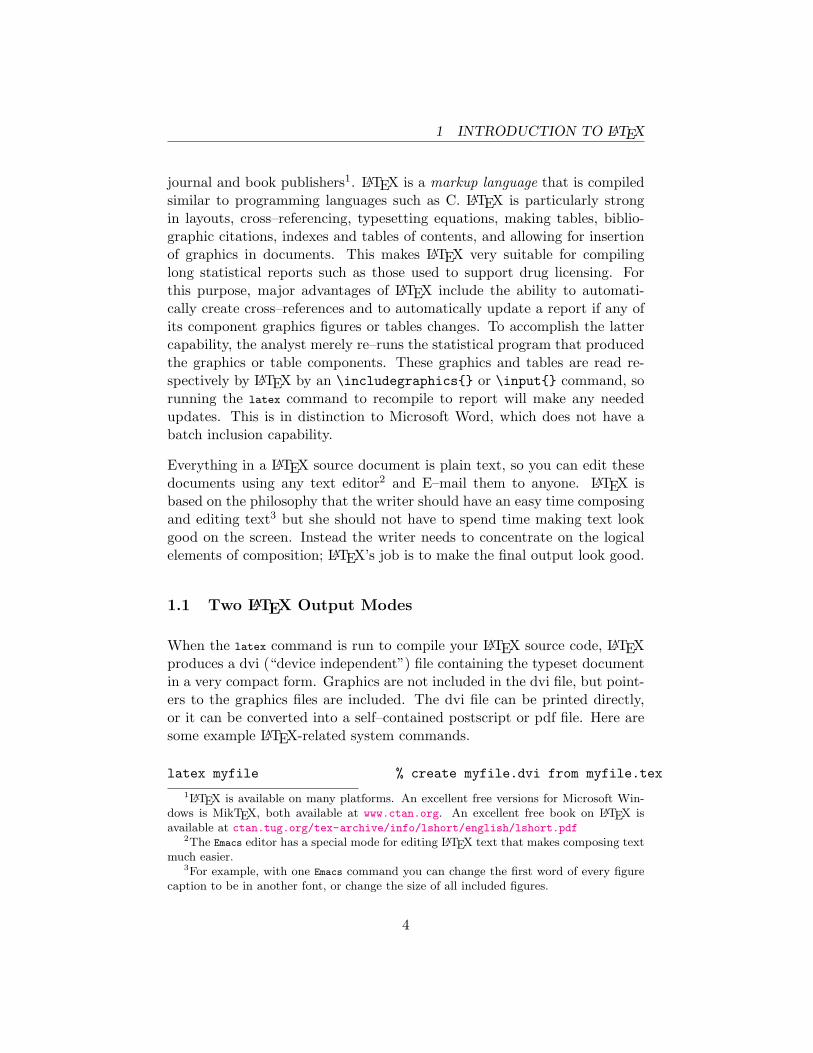
1 Introduction to LATEX
LATEX is a public domain document processing system developed by Lam-port (which uses TEX by Knuth) that is used heavily in the sciences and by
3
1 INTRODUCTION TO LATEX
journal and book publishers1. LATEX is a markup language that is compiledsimilar to programming languages such as C. LATEX is particularly strongin layouts, cross–referencing, typesetting equations, making tables, biblio-graphic citations, indexes and tables of contents, and allowing for insertionof graphics in documents. This makes LATEX very suitable for compilinglong statistical reports such as those used to support drug licensing. Forthis purpose, major advantages of LATEX include the ability to automati-cally create cross–references and to automatically update a report if any ofits component graphics figures or tables changes. To accomplish the lattercapability, the analyst merely re–runs the statistical program that producedthe graphics or table components. These graphics and tables are read re-spectively by LATEX by an \includegraphics{} or \input{} command, sorunning the latex command to recompile to report will make any neededupdates. This is in distinction to Microsoft Word, which does not have abatch inclusion capability.
Everything in a LATEX source document is plain text, so you can edit thesedocuments using any text editor2 and E–mail them to anyone. LATEX isbased on the philosophy that the writer should have an easy time composingand editing text3 but she should not have to spend time making text lookgood on the screen. Instead the writer needs to concentrate on the logicalelements of composition; LATEX’s job is to make the final output look good.
1.1 Two LATEX Output Modes
When the latex command is run to compile your LATEX source code, LATEXproduces a dvi (“device independent”) file containing the typeset documentin a very compact form. Graphics are not included in the dvi file, but point-ers to the graphics files are included. The dvi file can be printed directly,or it can be converted into a self–contained postscript or pdf file. Here aresome example LATEX-related system commands.
latex myfile % create myfile.dvi from myfile.tex
1LATEX is available on many platforms. An excellent free versions for Microsoft Win-dows is MikTEX, both available at www.ctan.org. An excellent free book on LATEX isavailable at ctan.tug.org/tex-archive/info/lshort/english/lshort.pdf
2The Emacs editor has a special mode for editing LATEX text that makes composing textmuch easier.
3For example, with one Emacs command you can change the first word of every figurecaption to be in another font, or change the size of all included figures.
4

1 INTRODUCTION TO LATEX
dvips myfile % send myfile to a postscript printerdvips -o myfile.ps myfile % convert myfile.dvi to myfile.ps, with
% graphicsdvips -Pwww -o myfile.ps myfile % use Type 1 fontsdvipdfm myfile % convert myfile.dvi to myfile.pdfpdflatex myfile % creates myfile.pdf directly if no
% postscript graphics are referenced
Creation of a static document in one of these ways is the usual mode of LATEXusage. There is also a way of using LATEX to create “live” documents thatare viewed on a monitor (either locally or over the web) or printed. Thesepdf documents may contain bookmarks, hyperlinks to external URLs, linksto E–mail addresses, etc. If you use the hyperref package in LATEX, thesystem will automatically make all pertinent elements of your documentcross–indexed and hyperlinked, and you can also insert special commandsto link to areas outside the document such as URLs and E–mail.
When viewing the document using Adobe Acrobat Reader, bookmarks canappear in the left margin, allowing the user to click to jump to any ma-jor section of the document. Sections having sub–sections can have theirbookmarks expanded so that you can jump to the sub–sections. You canjump to any figure while viewing the List of Figures and to any table whileviewing the List of Tables, in addition to jumping to any area while viewingthe Table of Contents. If your document is indexed, you can jump to anypage for which an indexed phrase is discussed. You can optionally jumpto pages in which a given article is cited while viewing the Bibliography, inaddition to the more standard jump from a citation to the bibliographicreference. If the colorlinks option is selected (see code below), symbols thatare hyperlinked appear in color; clicking on them will cause the jump. Allof this is set up automatically by hyperref, unlike the large number of flagsthat must be put in a document manually if using Microsoft Word.
Instead of compiling the document using the latex system command, youuse the pdflatex command to create the pdf file directly, with all bookmarksand hyperlinks.
This document was created in the fashion just described. PDF graphics fileswere created directly using an S pdf device driver. Below you will find thecode in the preamble of the document that set up the pdf document withhyper–referencing.
5
1 INTRODUCTION TO LATEX
\usepackage[pdftex,bookmarks,pagebackref,colorlinks,pdfpagemode=UseOutlines,pdfauthor={Frank E Harrell Jr},pdftitle={Statistical Tables and Plots using S and LaTeX}]{hyperref}
1.2 Basic Table Making in LATEX
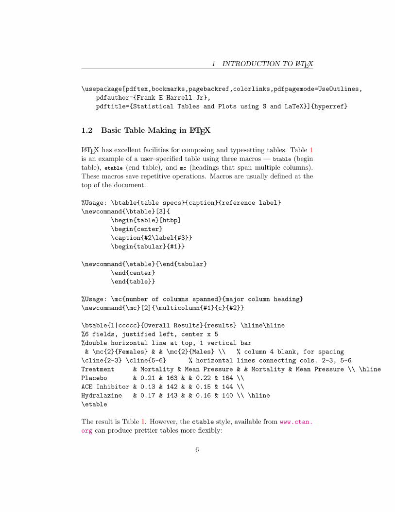
LATEX has excellent facilities for composing and typesetting tables. Table 1is an example of a user–specified table using three macros — btable (begintable), etable (end table), and mc (headings that span multiple columns).These macros save repetitive operations. Macros are usually defined at thetop of the document.
%Usage: \btable{table specs}{caption}{reference label}\newcommand{\btable}[3]{
\begin{table}[htbp]\begin{center}\caption{#2\label{#3}}\begin{tabular}{#1}}
\newcommand{\etable}{\end{tabular}\end{center}\end{table}}
%Usage: \mc{number of columns spanned}{major column heading}\newcommand{\mc}[2]{\multicolumn{#1}{c}{#2}}
\btable{l|ccccc}{Overall Results}{results} \hline\hline%6 fields, justified left, center x 5%double horizontal line at top, 1 vertical bar& \mc{2}{Females} & & \mc{2}{Males} \\ % column 4 blank, for spacing\cline{2-3} \cline{5-6} % horizontal lines connecting cols. 2-3, 5-6Treatment & Mortality & Mean Pressure & & Mortality & Mean Pressure \\ \hlinePlacebo & 0.21 & 163 & & 0.22 & 164 \\ACE Inhibitor & 0.13 & 142 & & 0.15 & 144 \\Hydralazine & 0.17 & 143 & & 0.16 & 140 \\ \hline\etable
The result is Table 1. However, the ctable style, available from www.ctan.org can produce prettier tables more flexibly:
6

2 USING S TO FILL IN CELLS IN LATEX TABLES
Table 1: Overall Results
Females MalesTreatment Mortality Mean Pressure Mortality Mean PressurePlacebo 0.21 163 0.22 164ACE Inhibitor 0.13 142 0.15 144Hydralazine 0.17 143 0.16 140
\ctable[caption={Overall Results},label=resultsb,pos=hbp!]{lccccc}{}{\FL& \mc{2}{Females} & & \mc{2}{Males} \NN\cmidrule{2-3}\cmidrule{5-6} % Important: no space before \cmidruleTreatment & Mortality & Mean Pressure & & Mortality & Mean Pressure \MLPlacebo & 0.21 & 163 & & 0.22 & 164 \NNACE Inhibitor & 0.13 & 142 & & 0.15 & 144 \NNHydralazine & 0.17 & 143 & & 0.16 & 140 \LL}
The result is shown in Table 2.
Table 2: Overall Results
Females Males
Treatment Mortality Mean Pressure Mortality Mean Pressure
Placebo 0.21 163 0.22 164ACE Inhibitor 0.13 142 0.15 144Hydralazine 0.17 143 0.16 140
2 Using S to Fill in Cells in LATEX Tables
For most statistical tables a better idea is to avoid transcription of calculatedvalues by having the values inserted into tables automatically. The Hmisc
7
2 USING S TO FILL IN CELLS IN LATEX TABLES
library (see biostat.mc.vanderbilt.edu/Hmisc) contains several S func-tions by R Heiberger and F Harrell that automatically make LATEX tablesfrom S objects4. S functions that automatically produce LATEX code fromS objects (matrices, fitted models, data summaries, etc.) have names thatstart with latex. Tables produced by the latex.* functions in Hmisc meetthe stylistic requirements of most journals, i.e., by default they do not usevertical lines and they use horizontal lines only when needed. In this waythe lines do not distract from delivering the statistical information.
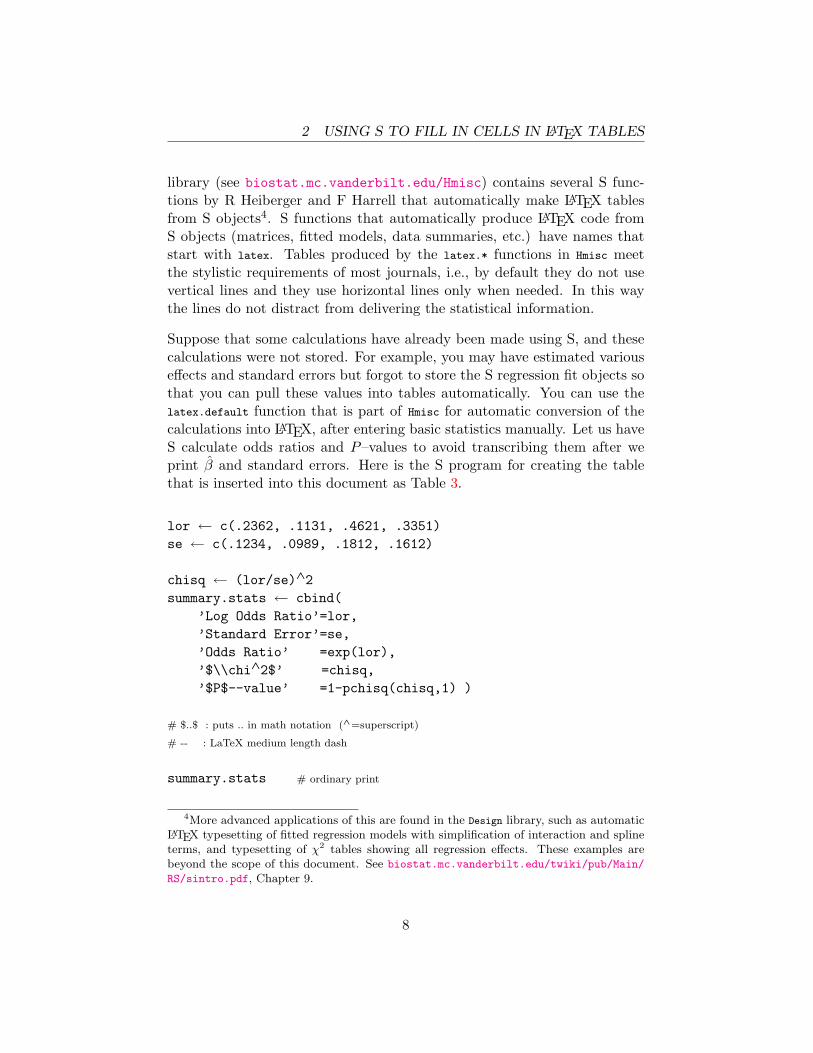
Suppose that some calculations have already been made using S, and thesecalculations were not stored. For example, you may have estimated variouseffects and standard errors but forgot to store the S regression fit objects sothat you can pull these values into tables automatically. You can use thelatex.default function that is part of Hmisc for automatic conversion of thecalculations into LATEX, after entering basic statistics manually. Let us haveS calculate odds ratios and P–values to avoid transcribing them after weprint β̂ and standard errors. Here is the S program for creating the tablethat is inserted into this document as Table 3.
lor ← c(.2362, .1131, .4621, .3351)se ← c(.1234, .0989, .1812, .1612)
chisq ← (lor/se)∧2summary.stats ← cbind(
’Log Odds Ratio’=lor,’Standard Error’=se,’Odds Ratio’ =exp(lor),’$\\chi∧2$’ =chisq,’$P$--value’ =1-pchisq(chisq,1) )
# $..$ : puts .. in math notation (∧=superscript)
# -- : LaTeX medium length dash
summary.stats # ordinary print
4More advanced applications of this are found in the Design library, such as automaticLATEX typesetting of fitted regression models with simplification of interaction and splineterms, and typesetting of χ2 tables showing all regression effects. These examples arebeyond the scope of this document. See biostat.mc.vanderbilt.edu/twiki/pub/Main/
RS/sintro.pdf, Chapter 9.
8
2 USING S TO FILL IN CELLS IN LATEX TABLES
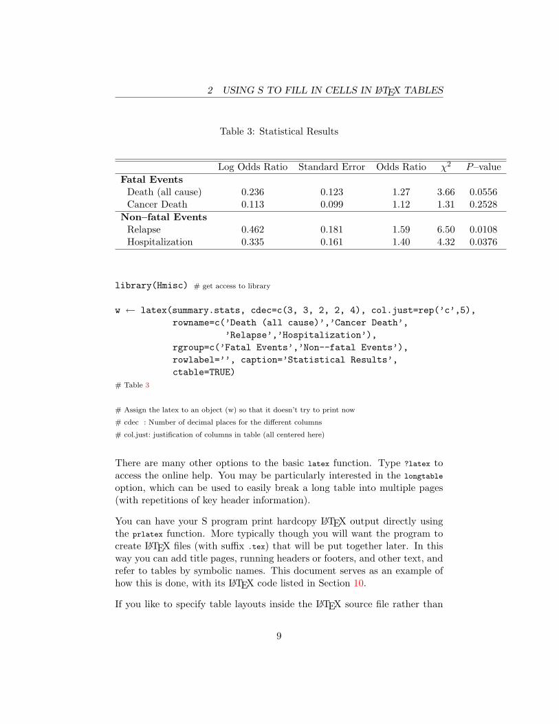
Table 3: Statistical Results
Log Odds Ratio Standard Error Odds Ratio χ2 P–valueFatal Events
Death (all cause) 0.236 0.123 1.27 3.66 0.0556Cancer Death 0.113 0.099 1.12 1.31 0.2528
Non–fatal EventsRelapse 0.462 0.181 1.59 6.50 0.0108Hospitalization 0.335 0.161 1.40 4.32 0.0376
library(Hmisc) # get access to library
w ← latex(summary.stats, cdec=c(3, 3, 2, 2, 4), col.just=rep(’c’,5),rowname=c(’Death (all cause)’,’Cancer Death’,
’Relapse’,’Hospitalization’),rgroup=c(’Fatal Events’,’Non--fatal Events’),rowlabel=’’, caption=’Statistical Results’,ctable=TRUE)
# Table 3
# Assign the latex to an object (w) so that it doesn’t try to print now
# cdec : Number of decimal places for the different columns
# col.just: justification of columns in table (all centered here)
There are many other options to the basic latex function. Type ?latex toaccess the online help. You may be particularly interested in the longtable
option, which can be used to easily break a long table into multiple pages(with repetitions of key header information).
You can have your S program print hardcopy LATEX output directly usingthe prlatex function. More typically though you will want the program tocreate LATEX files (with suffix .tex) that will be put together later. In thisway you can add title pages, running headers or footers, and other text, andrefer to tables by symbolic names. This document serves as an example ofhow this is done, with its LATEX code listed in Section 10.
If you like to specify table layouts inside the LATEX source file rather than
9

3 USING S TO CREATE GRAPHICS FOR LATEX
inside S, you can have your S program output symbolic values to a file thatis \input{}’d in LATEX as shown in the following example. A restrictionis that variable names defined to LATEX may contain only letters and theyshould not coincide with names of LATEX commands.
chisq <- (beta/se)^2pval <- 1 - pchisq(chisq, 1)cat(’\\def\\chisq{’,round(chisq,2),’}\\n’, # \\ -> \ in parms.tex
’\\def\\pval{’,round(pval,4),’}\n’, sep=’’, file=’parms.tex’)
If LATEX variables are named the same as S variables, and the names containonly letters, code can be simplified using a little function. This function canalso convert NAs to blanks.
lvar <- function(x, digits=2)paste(’\\def\\’,substitute(x),’{’,
ifelse(is.na(x),’’,round(x,digits)),’}’, sep=’’)
cat(lvar(chisq), lvar(pval,4), sep=’\n’, file=’parms.tex’)
The contents of file parms.tex will look like the following:
\def\chisq{3.84}\def\pval{0.05}
Inside the main LATEX source file use for example
\input{parms}\ctable[caption={Main Results},label=resultsc]{lcc}{}{Test & $\chi^2$ & $P$--value \MLAge effect & \chisq & \pval \LL}
3 Using S to Create Graphics for LATEX
PostScript is a graphics format accepted by all versions of LATEX as longas you have a PostScript printer or have GhostScript or Adobe Acrobat
10
3 USING S TO CREATE GRAPHICS FOR LATEX
Distiller to convert postscript output to other formats. The basic graphicsdriver in S for creating postscript files is the postscript function. For creating35mm slides, overhead transparencies, or 5 × 7 glossy figures, the ps.slide
function in the Hmisc library assists in setting up nice defaults for postscriptimages. For reports and books, the Hmisc setps function makes creating ofindividual postscript graphics easy5. setps uses reasonable defaults and setsup for a minimally sized bounding box. It tries not to waste space betweenaxes and axis labels. In the following example, a file called test.ps is createdin the current working directory. Note the absence of quote marks aroundthe word test below.
setps(test) # use setps(test, trellis=T) if using Trellis (R Lattice)
plot(....)dev.off() # close file, creating test.ps
As you will see later, we can symbolically label this figure using the word test
in LATEX. By default, setps uses Helvetica font and makes small book–stylefigures. There are many options to override these and other settings.
If you are using pdflatex, graphics files must be in Adobe pdf format. Youcan create pdf files directly in S-Plus using the builtin pdf.graph function,in R using the pdf function, or using the Hmisc setpdf function. In olderversions of S-Plus, better results are obtained by creating postscript andconverting the graph to pdf. If you have Ghostscript installed and have usedsetps followed by dev.off, you can type topdf() with no arguments to invokeGhostscript from S to create, in this case, test.pdf. You can also convertfrom postscript to pdf using Adobe Acrobat Distiller, which produces morecompact pdf files. In R, direct creation of .pdf files seems to work well.
3.1 Inserting Graphics Files into LATEX Documents
The standard graphics and graphicx packages in LATEX provide all you need toinsert postscript and pdf graphics into a document in a flexible fashion. Thisis not to say that it is as easy as using Word; frequently some trial and erroris required to get graphics to have an appropriate scaling (magnification)
5The corresponding Hmisc function for creating pdf files is setpdf. You can also usethe postscript and pdf functions directly. Some useful templates for doing so may befound at http://biostat.mc.vanderbilt.edu/SgraphicsHints.
11
4 MAKING S COMPOSE LATEX TABLES
factor. Inclusion of pdf graphics in older versions of S-Plus and LATEXfrequently resulted in much wasted spaced before and after the graph whenusing pdflatex, so you often had to use \vspace commands with negativearguments when including pdf files.
Here is a LATEX macro for inserting pdf graphics files, which are assumed tohave a .pdf suffix.
% Usage: \fig{label=.pdf prefix}{caption}{short caption for list of% figures}{scalefactor}\newcommand{\fig}[4]{\begin{figure}[hbp!]\leavevmode\centerline{\includegraphics[scale=#4]{#1.pdf}}\caption[#3]{\small #2}\label{#1}\end{figure}}
For example, \fig{test}{long caption}{short caption}{.8} will inserttest.pdf and reduce its size by 20%. You can refer to this figure in the textusing for example see Figure~\ref{test}.
4 Making S Compose LATEX Tables
In many cases S functions can be used to make all calculations for the tableand then to create the LATEX table. Harrell’s S summary function for formu-las (actually summary.formula) is one function that will do this when whatyou need is descriptive statistics (including statistics computed by func-tions you create). summary is in the Hmisc library available at biostat.mc.vanderbilt.edu/Hmisc. It has three methods for computing descriptivestatistics on univariate or multivariate responses, subsetted by categoriesof other variables. See An Introduction to S and the Hmisc and Design Li-braries by CF Alzola and FE Harrell (biostat.mc.vanderbilt.edu/twiki/pub/Main/RS/sintro.pdf) for more information about summary.formula andS usage in general, especially information on how to recode and reshape datato be used in reports.
The output from summary.formula can be printed (for ordinary text file print-outs), plotted (dot charts or occasionally box-percentile plots), or typesetusing LATEX, as there are several print, plot, and latex methods for objects
12
4 MAKING S COMPOSE LATEX TABLES
created by summary.formula. The latex methods create all the needed table el-ements, then invoke the latex.default method in Hmisc to build the completeset of LATEX commands to make each table.
The method of data summarization to be done by summary.formula is specifiedin the parameter method. These methods are defined below. For the first andthird methods, the statistics used to summarize the data may be specified ina flexible manner by the user (e.g., the geometric mean, 33rd percentile, orKaplan–Meier 2–year survival estimate, mixtures of several statistics). Thedefault summary statistic is the mean, which for a binary response variableis the proportion of positive responses.
method=’response’: The response variable may be multivariate, and any num-ber of statistics may be used to summarize the responses. Sometimesdependent variables are multivariate because they indicate follow–uptime and censoring, and sometimes they are multivariate because thereare several response variables (e.g., systolic and diastolic blood pres-sure). The responses are summarized separately for each independentvariable (independent variables are not cross–classified). Continuousindependent variables are automatically stratified into quantile groups.One or more of the independent variables may be stratification fac-tors, in which all computations are done separately by levels of thesecategorical variables. The stratification variables form major columngroupings in tables. For multivariate responses, subjects are consid-ered to be missing if any response variable is missing.
method=’reverse’: This format is typical of baseline characteristic tables de-scribing the usual success of randomization. Here the single dependentvariable must be categorical (e.g., treatment assignment), and the “in-dependent” variables are broken down separately by the dependentvariable. Continuous independent variables are described by threequantiles (quartiles by default), and categorical ones are described bycounts and percentages. There is an option to automatically generatetest statistics for testing across columns of ’reverse’ tables.
method=’cross’: The ’cross’ method allows allows for multiple dependentvariables and multiple statistics to summarize each one. If there ismore than one independent variable (up to three is allowed), statisticsare computed separately for all cross–classifications of the indepen-dent variables, and marginal and overall statistics may optionally be
13
4 MAKING S COMPOSE LATEX TABLES
computed. summary.formula for this method outputs a data frame con-taining the combinations of predictors along with the response sum-maries. This data frame may be summarized graphically in variousways using the S-Plus trellis library or R lattice package6. A LATEXprinting method, for the case where there is exactly two predictors,typesets a two–way table where the first predictor forms rows and thesecond forms columns. Like method=’response’, continuous variables areautomatically divided into quantile groups.
The latex methods in the Hmisc library create tables using standard LATEXcommands. These tables are inserted into the master document at the de-sired location using an \input{} command. latex methods allow a font size
argument. For example, you may specify size=’small’ to latex(), or you maywant to use a generic size that is set at LATEX run time in the documentpreamble. For example, specify \def\tsz{small} in the master documentand specify size=’tsz’ to latex(). Then you can define (and redefine) thesize for tables without modifying the individual .tex files created by latex().Another approach using LATEX’s relsize style is discussed on P. 35.
4.1 Reports Formatted to Describe Responses
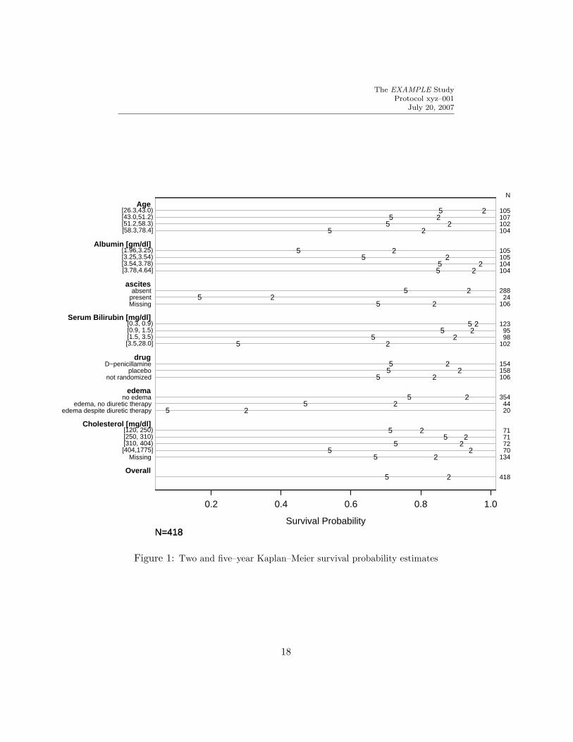
Tables 4–8 were produced by the S latex function (actually,latex.summary.formula.response), which is run on an object created by thesummary function with method=’response’, the default.
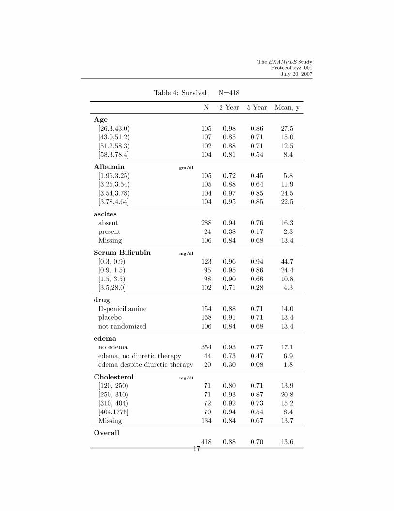
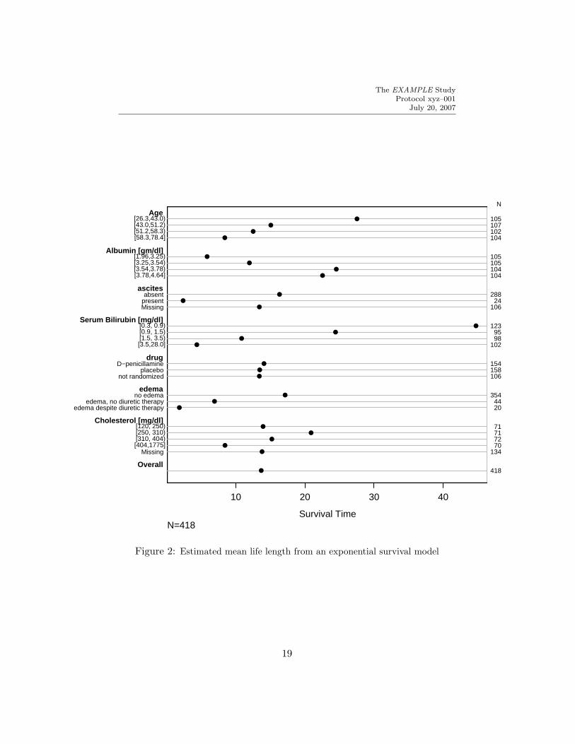
Table 4 presents Kaplan–Meier 2 and 5 year survival estimates and meanlife length of subjects in the Mayo Clinic primary biliary cirrhosis datasetavailable from biostat.mc.vanderbilt.edu/DataSets. The calculationsare subsetted on various patient characteristics. For estimating mean lifelength, an exponential survival model was assumed (the estimate is years perevent). Continuous variables are categorized into quartiles automatically.Each quartile group is identified using the upper and lower endpoints withinthat quartile. The code for this example follows.
library(Hmisc)library(survival)
6For this purpose, the Hmisc summarize function may be more useful, if you don’t wantmarginal statistics computed.
14
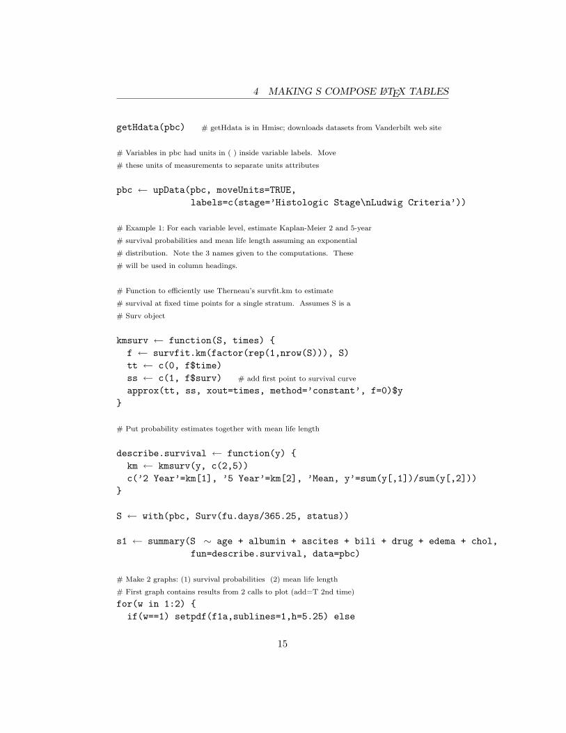
4 MAKING S COMPOSE LATEX TABLES
getHdata(pbc) # getHdata is in Hmisc; downloads datasets from Vanderbilt web site
# Variables in pbc had units in ( ) inside variable labels. Move
# these units of measurements to separate units attributes
pbc ← upData(pbc, moveUnits=TRUE,labels=c(stage=’Histologic Stage\nLudwig Criteria’))
# Example 1: For each variable level, estimate Kaplan-Meier 2 and 5-year
# survival probabilities and mean life length assuming an exponential
# distribution. Note the 3 names given to the computations. These
# will be used in column headings.
# Function to efficiently use Therneau’s survfit.km to estimate
# survival at fixed time points for a single stratum. Assumes S is a
# Surv object
kmsurv ← function(S, times) {f ← survfit.km(factor(rep(1,nrow(S))), S)tt ← c(0, f$time)ss ← c(1, f$surv) # add first point to survival curve
approx(tt, ss, xout=times, method=’constant’, f=0)$y}
# Put probability estimates together with mean life length
describe.survival ← function(y) {km ← kmsurv(y, c(2,5))c(’2 Year’=km[1], ’5 Year’=km[2], ’Mean, y’=sum(y[,1])/sum(y[,2]))
}
S ← with(pbc, Surv(fu.days/365.25, status))
s1 ← summary(S ∼ age + albumin + ascites + bili + drug + edema + chol,fun=describe.survival, data=pbc)
# Make 2 graphs: (1) survival probabilities (2) mean life length
# First graph contains results from 2 calls to plot (add=T 2nd time)
for(w in 1:2) {if(w==1) setpdf(f1a,sublines=1,h=5.25) else
15

The EXAMPLE StudyProtocol xyz–001
July 20, 2007
setpdf(f1b,sublines=1,h=5)plot(s1, which=if(w==1)1:2 else 3,
cex.labels=.7, cex.group.labels=.7*1.15, subtitles=T, main=’’,pch=if(w==2) 16 else c(’2’,’5’), # 16=solid circle
xlab=if(w==2)’Survival Time’ else ’Survival Probability’)dev.off()
}
w ← latex(s1, cdec=c(2,2,1), ctable=TRUE, caption=’Survival’)# Creates s1.tex (Table 4)
This table is converted to two dot plots (Figures 1 and 2) using the plot
method for an object created by summary with method=’response’ (see previouscode). The Hmisc setpdf function is used to create the pdf graphics files.See Section 10 for the LATEX code used to insert these graphics.
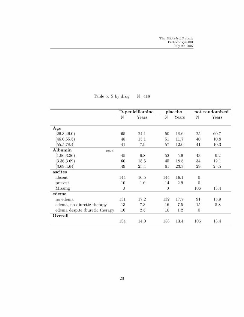
Table 5 is similar to Table 4 except that the Kaplan–Meier estimates are notshown, life length estimates are also stratified by treatment assigned (usingthe stratify function), and continuous variables are grouped into tertiles.
# Example 2: Stratify mean life length (only) by drug groups. These will
# become major column groupings. Use tertiles instead of quartiles.
life.expect ← function(y) c(Years=sum(y[,1])/sum(y[,2]))
s2 ← summary(S ∼ age + albumin + ascites + edema + stratify(drug),fun=life.expect, g=3, data=pbc)
# Note: You can summarize other response variables using the same independent
# variables using e.g. update(s2, response∼.), or you can change the
# list of independent variables using e.g. update(s2, response ∼.- ascites)
# or update(s2, .∼.-ascites)
setpdf(f2, h=4)plot(s2, cex.labels=.6, xlim=c(0,40), # Figure 3
xlab=’Mean Life Length’, main=’’)Key(-.09,.05)dev.off()
w ← latex(s2, cdec=1, ctable=TRUE)
16
The EXAMPLE StudyProtocol xyz–001
July 20, 2007
Table 4: Survival N=418
N 2 Year 5 Year Mean, y
Age[26.3,43.0) 105 0.98 0.86 27.5[43.0,51.2) 107 0.85 0.71 15.0[51.2,58.3) 102 0.88 0.71 12.5[58.3,78.4] 104 0.81 0.54 8.4
Albumin gm/dl
[1.96,3.25) 105 0.72 0.45 5.8[3.25,3.54) 105 0.88 0.64 11.9[3.54,3.78) 104 0.97 0.85 24.5[3.78,4.64] 104 0.95 0.85 22.5
ascitesabsent 288 0.94 0.76 16.3present 24 0.38 0.17 2.3Missing 106 0.84 0.68 13.4
Serum Bilirubin mg/dl
[0.3, 0.9) 123 0.96 0.94 44.7[0.9, 1.5) 95 0.95 0.86 24.4[1.5, 3.5) 98 0.90 0.66 10.8[3.5,28.0] 102 0.71 0.28 4.3
drugD-penicillamine 154 0.88 0.71 14.0placebo 158 0.91 0.71 13.4not randomized 106 0.84 0.68 13.4
edemano edema 354 0.93 0.77 17.1edema, no diuretic therapy 44 0.73 0.47 6.9edema despite diuretic therapy 20 0.30 0.08 1.8
Cholesterol mg/dl
[120, 250) 71 0.80 0.71 13.9[250, 310) 71 0.93 0.87 20.8[310, 404) 72 0.92 0.73 15.2[404,1775] 70 0.94 0.54 8.4Missing 134 0.84 0.67 13.7
Overall418 0.88 0.70 13.6
17
The EXAMPLE StudyProtocol xyz–001
July 20, 2007
Survival Probability
0.2 0.4 0.6 0.8 1.0
22
22
22
22
22
2
22
22
22
2
22
2
22
22
2
2
105 107 102 104
105 105 104 104
288 24
106
123 95 98
102
154 158 106
354 44 20
71 71 72 70
134
418
N
absent present Missing
D−penicillamine placebo
not randomized
no edema edema, no diuretic therapy
edema despite diuretic therapy
Missing
[26.3,43.0) [43.0,51.2) [51.2,58.3) [58.3,78.4]
[1.96,3.25) [3.25,3.54) [3.54,3.78) [3.78,4.64]
[0.3, 0.9) [0.9, 1.5) [1.5, 3.5) [3.5,28.0]
[120, 250) [250, 310) [310, 404) [404,1775]
Age
Albumin [gm/dl]
ascites
Serum Bilirubin [mg/dl]
drug
edema
Cholesterol [mg/dl]
Overall
N=418
55
55
55
55
55
5
55
55
55
5
55
5
55
55
5
5
N=418
Figure 1: Two and five–year Kaplan–Meier survival probability estimates
18
The EXAMPLE StudyProtocol xyz–001
July 20, 2007
Survival Time
10 20 30 40
●
●
●
●
●
●
●
●
●
●
●
●
●
●
●
●
●
●
●
●
●
●
●
●
●
●
●
105 107 102 104
105 105 104 104
288 24
106
123 95 98
102
154 158 106
354 44 20
71 71 72 70
134
418
N
absent present Missing
D−penicillamine placebo
not randomized
no edema edema, no diuretic therapy
edema despite diuretic therapy
Missing
[26.3,43.0) [43.0,51.2) [51.2,58.3) [58.3,78.4]
[1.96,3.25) [3.25,3.54) [3.54,3.78) [3.78,4.64]
[0.3, 0.9) [0.9, 1.5) [1.5, 3.5) [3.5,28.0]
[120, 250) [250, 310) [310, 404) [404,1775]
Age
Albumin [gm/dl]
ascites
Serum Bilirubin [mg/dl]
drug
edema
Cholesterol [mg/dl]
Overall
N=418
Figure 2: Estimated mean life length from an exponential survival model
19
The EXAMPLE StudyProtocol xyz–001
July 20, 2007
Table 5: S by drug N=418
D-penicillamine placebo not randomizedN Years N Years N Years
Age[26.3,46.0) 65 24.1 50 18.6 25 60.7[46.0,55.5) 48 13.1 51 11.7 40 10.8[55.5,78.4] 41 7.9 57 12.0 41 10.3
Albumin gm/dl
[1.96,3.36) 45 6.8 52 5.9 43 9.2[3.36,3.69) 60 15.5 45 18.8 34 12.1[3.69,4.64] 49 25.4 61 23.3 29 25.5
ascitesabsent 144 16.5 144 16.1 0present 10 1.6 14 2.9 0Missing 0 0 106 13.4
edemano edema 131 17.2 132 17.7 91 15.9edema, no diuretic therapy 13 7.3 16 7.5 15 5.8edema despite diuretic therapy 10 2.5 10 1.2 0
Overall154 14.0 158 13.4 106 13.4
20

The EXAMPLE StudyProtocol xyz–001
July 20, 2007
This table is converted to a dot plot in Figure 3.
Mean Life Length
0 10 20 30 40
●
●
●
●
●
●
●
●
●
●
●
●
140
139
139
140
139
139
288
24
106
354
44
20
418
N
absent
present
Missing
no edema
edema, no diuretic therapy
edema despite diuretic therapy
[26.3,46.0)
[46.0,55.5)
[55.5,78.4]
[1.96,3.36)
[3.36,3.69)
[3.69,4.64]
Age
Albumin [gm/dl]
ascites
edema
Overall
●
●
●
●
●
●
●
●
●
●
●
●
●
●
D−penicillamineplacebonot randomized
Figure 3: Estimated mean life length from an exponential survival model
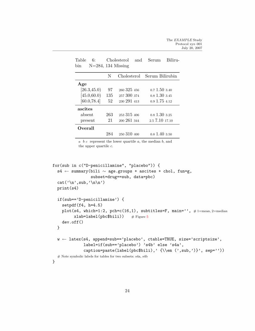
Table 6 displays quartiles of cholesterol and bilirubin by various patientcharacteristics. To compute statistics simultaneously for cholesterol andbilirubin, we must use the S cbind function to create a bivariate responsevariable (a 2–column matrix). To compute quantiles for this new 2–variableentity we have to use the apply function instead of a simple invocation toquantile. For age, pre–specified intervals are used.
# Example 3: Take control of groups used for age. Compute 3 quartiles for
21
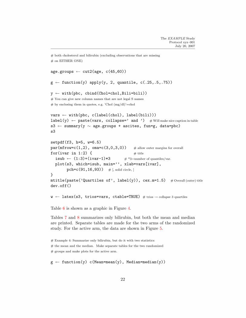
The EXAMPLE StudyProtocol xyz–001
July 20, 2007
# both cholesterol and bilirubin (excluding observations that are missing
# on EITHER ONE)
age.groups ← cut2(age, c(45,60))
g ← function(y) apply(y, 2, quantile, c(.25,.5,.75))
y ← with(pbc, cbind(Chol=chol,Bili=bili))# You can give new column names that are not legal S names
# by enclosing them in quotes, e.g. ’Chol (mg/dl)’=chol
vars ← with(pbc, c(label(chol), label(bili)))label(y) ← paste(vars, collapse=’ and ’) # Will make nice caption in table
s3 ← summary(y ∼ age.groups + ascites, fun=g, data=pbc)s3
setpdf(f3, h=5, w=6.5)par(mfrow=c(1,2), oma=c(3,0,3,0)) # allow outer margins for overall
for(ivar in 1:2) { # title
isub ← (1:3)+(ivar-1)*3 # *3=number of quantiles/var.
plot(s3, which=isub, main=’’, xlab=vars[ivar],pch=c(91,16,93)) # [, solid circle, ]
}mtitle(paste(’Quartiles of’, label(y)), cex.m=1.5) # Overall (outer) title
dev.off()
w ← latex(s3, trios=vars, ctable=TRUE) # trios → collapse 3 quartiles
Table 6 is shown as a graphic in Figure 4.
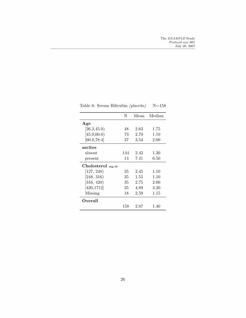
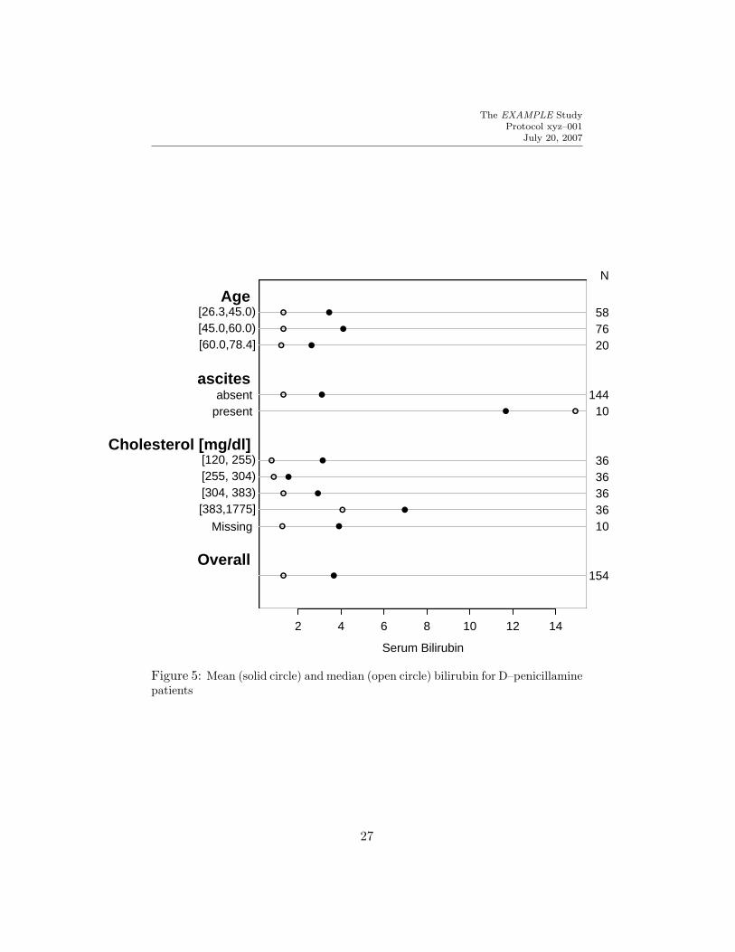
Tables 7 and 8 summarizes only bilirubin, but both the mean and medianare printed. Separate tables are made for the two arms of the randomizedstudy. For the active arm, the data are shown in Figure 5.
# Example 4: Summarize only bilirubin, but do it with two statistics:
# the mean and the median. Make separate tables for the two randomized
# groups and make plots for the active arm.
g ← function(y) c(Mean=mean(y), Median=median(y))
22

The EXAMPLE StudyProtocol xyz–001
July 20, 2007
Cholesterol
200 250 300 350 400 450
[
[
[
[
[
[
97
135
52
263
21
284
N
absent
present
[26.3,45.0)
[45.0,60.0)
[60.0,78.4]
Age
ascites
Overall
N=284 N missing=134
●
●
●
●
●
●
N=284 N missing=134
]
]
]
]
]
]
N=284 N missing=134Serum Bilirubin
5 10 15
[
[
[
[
[
[
97
135
52
263
21
284
N
absent
present
[26.3,45.0)
[45.0,60.0)
[60.0,78.4]
Age
ascites
Overall
N=284 N missing=134
●
●
●
●
●
●
N=284 N missing=134
]
]
]
]
]
]
N=284 N missing=134
Quartiles of Cholesterol and Serum Bilirubin
19Jul07
Figure 4: Quartiles of cholesterol and bilirubin
23
The EXAMPLE StudyProtocol xyz–001
July 20, 2007
Table 6: Cholesterol and Serum Biliru-bin N=284, 134 Missing
N Cholesterol Serum Bilirubin
Age[26.3,45.0) 97 260 325 456 0.7 1.50 3.40
[45.0,60.0) 135 257 300 374 0.8 1.30 3.45
[60.0,78.4] 52 230 291 413 0.9 1.75 4.12
ascitesabsent 263 253 315 406 0.8 1.30 3.25
present 21 200 261 344 2.5 7.10 17.10
Overall284 250 310 400 0.8 1.40 3.50
a b c represent the lower quartile a, the median b, andthe upper quartile c.
for(sub in c("D-penicillamine", "placebo")) {s4 ← summary(bili ∼ age.groups + ascites + chol, fun=g,
subset=drug==sub, data=pbc)cat(’\n’,sub,’\n\n’)print(s4)
if(sub==’D-penicillamine’) {setpdf(f4, h=4.5)plot(s4, which=1:2, pch=c(16,1), subtitles=F, main=’’, # 1=mean, 2=median
xlab=label(pbc$bili)) # Figure 5
dev.off()}
w ← latex(s4, append=sub==’placebo’, ctable=TRUE, size=’scriptsize’,label=if(sub==’placebo’) ’s4b’ else ’s4a’,caption=paste(label(pbc$bili),’ {\\em (’,sub,’)}’, sep=’’))
# Note symbolic labels for tables for two subsets: s4a, s4b
}
24

The EXAMPLE StudyProtocol xyz–001
July 20, 2007
Table 7: Serum Bilirubin (D-penicillamine) N=154
N Mean Median
Age[26.3,45.0) 58 3.43 1.30[45.0,60.0) 76 4.09 1.30[60.0,78.4] 20 2.61 1.20
ascitesabsent 144 3.09 1.30present 10 11.66 14.90
Cholesterol mg/dl
[120, 255) 36 3.13 0.75[255, 304) 36 1.54 0.85[304, 383) 36 2.91 1.30[383,1775] 36 6.96 4.05Missing 10 3.89 1.25
Overall154 3.65 1.30
25
The EXAMPLE StudyProtocol xyz–001
July 20, 2007
Table 8: Serum Bilirubin (placebo) N=158
N Mean Median
Age[26.3,45.0) 48 2.63 1.75[45.0,60.0) 73 2.70 1.10[60.0,78.4] 37 3.54 2.00
ascitesabsent 144 2.43 1.30present 14 7.41 6.50
Cholesterol mg/dl
[127, 248) 35 2.45 1.10[248, 316) 35 1.55 1.10[316, 420) 35 2.75 2.00[420,1712] 35 4.89 3.20Missing 18 2.59 1.15
Overall158 2.87 1.40
26
The EXAMPLE StudyProtocol xyz–001
July 20, 2007
Serum Bilirubin
2 4 6 8 10 12 14
●
●
●
●
●
●
●
●
●
●
●
58 76 20
144 10
36 36 36 36 10
154
N
absent present
Missing
[26.3,45.0) [45.0,60.0) [60.0,78.4]
[120, 255) [255, 304) [304, 383) [383,1775]
Age
ascites
Cholesterol [mg/dl]
Overall
●
●
●
●
●
●
●
●
●
●
●
Figure 5: Mean (solid circle) and median (open circle) bilirubin for D–penicillaminepatients
27
The EXAMPLE StudyProtocol xyz–001
July 20, 2007
4.2 Baseline Characteristic Tables
Here the S summary function is used with the parameter method=’reverse’,which reverses the role of the dependent variable and the independent vari-ables. The dependent variable is assumed to be categorical; in clinical trialsit will be the treatment assignment.
The next example again uses the primary biliary cirrhosis dataset. Theresult is in Table 9. It is printed in landscape mode using the LATEXlscape package, and using the LATEX relsize package for relative sizing. For’reverse’-type tables, an option test=TRUE will cause summary.formula to com-pute test statistics for testing across columns. Default tests are Wilcoxon orKruskal-Wallis for continuous variables and Pearson χ2 for categorical ones,but users may specify their own statistical tests7.
# Now consider examples in ’reverse’ format, where the lone dependent
# variable tells the summary function how to stratify all the ’independent’
# variables. This is typically used to make tables comparing baseline
# variables by treatment group, for example.
s5 ← summary(drug ∼ bili + albumin + stage + protime + sex + age + spiders,method=’reverse’, dta=pbc, test=TRUE)
# To summarize all variables, use summary(drug ∼., data=pbc)
options(digits=1)print(s5, npct=’both’)# npct=’both’ : print both numerators and denominators
options(digits=3)w ← latex(s5, size=’smaller’, npct=’both’,
npct.size=’smaller[2]’, Nsize=’smaller[2]’,msdsize=’smaller[2]’,middle.bold=TRUE, landscape=TRUE)
# Note use of relative sizes throughout
# Specify prtest=’P’ to just print P-values, prtest=’stat’ to just
# print test statistics
w$style ← c(w$style, ’relsize’) # needed for preview only
7In randomized trials, tests for baseline imbalance are unwarranted, difficult to inter-pret, result in inappropriate actions, and cause multiple comparison problems (see StephenSenn, Statistical Issues in Drug Development).
28

The EXAMPLE StudyProtocol xyz–001
July 20, 2007
setpdf(f5a, h=7, pointsize=14)plot(s5, which=’categorical’) # Figure 6
Key(-.08,.5)dev.off()setpdf(f5b, h=7, pointsize=10)# Use box-percentile plot option
plot(s5, which=’continuous’, conType=’bp’) # Figure 7
dev.off()
# Repeat, dropping group of nonrandomized subjects so can get micro dotcharts
s5a ← summary(drug ∼ bili + albumin + stage + protime + sex + age + spiders,method=’reverse’, data=pbc, subset=drug!=’not randomized’,test=TRUE)
options(digits=1)print(s5a, npct=’both’)# npct=’both’ : print both numerators and denominators
options(digits=3)w ← latex(s5a, npct=’both’, landscape=TRUE,
dotchart=TRUE, middle.bold=TRUE)
29

Table 9: Descriptive Statistics by drug
N D-penicillamine placebo not randomized Test StatisticN = 154 N = 158 N = 106
Serum Bilirubin mg/dl 418 0.725 1.300 3.600 0.800 1.400 3.200 0.725 1.400 3.075 F2,415 = 0.03, P = 0.9721
Albumin gm/dl 418 3.34 3.54 3.78 3.21 3.56 3.83 3.12 3.47 3.72 F2,415 = 2.13, P = 0.121
Histologic Stage Ludwig Criteria : 1 412 3% 4154 8% 12
158 5% 5100 χ2
6 = 5.33, P = 0.5022
2 21% 32154 22% 35
158 25% 25100
3 42% 64154 35% 56
158 35% 35100
4 35% 54154 35% 55
158 35% 35100
Prothrombin Time sec. 416 10.0 10.6 11.4 10.0 10.6 11.0 10.1 10.6 11.0 F2,413 = 0.23, P = 0.7951
sex : female 418 90% 139154 87% 137
158 92% 98106 χ2
2 = 2.38, P = 0.3042
Age 418 41.4 48.1 55.8 43.0 51.9 58.9 46.0 53.0 61.0 F2,415 = 6.1, P = 0.0021
spiders 312 29% 45154 28% 45
158 χ21 = 0.02, P = 0.8852
a b c represent the lower quartile a, the median b, and the upper quartile c for continuous variables.N is the number of non–missing values.Tests used: 1Kruskal-Wallis test; 2Pearson test
The EXAMPLE StudyProtocol xyz–001
July 20, 2007
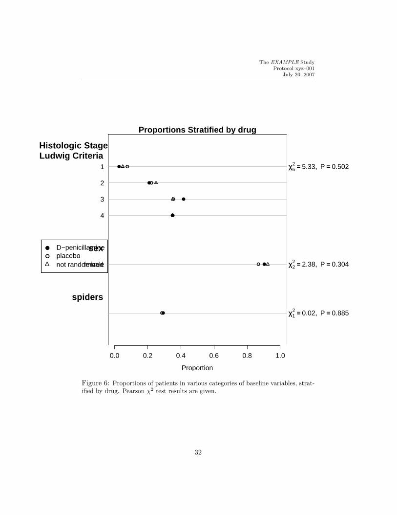
To convert Table 9 to graphical form, plot.summary.formula.reverse constructstwo pages. The first page contains statistics for all of the categorical vari-ables, as all of these statistics are on the same scale (proportion or percentin each category). The second page contains a matrix of dot charts showing(by default) the 3 quartiles of each right–hand–side variable (on the x–axis),stratified by the left–hand variable (on the y–axis of each dot plot). The sec-ond set of plots is scaled to the most extreme 0.025 to 0.975 quantiles of thevariable over all treatment groups. R can plot Greek letters, superscripts,subscripts, and mathematical operators, and Figure 6 and 7 take advantageof this capability. S-Plus does not have this capability, so simpler outputwould appear.
Table 10 with micrographs (micro dot charts) showing proportions is ob-tained as follows. These micrographs, implemented by Charles ThomasDupont of Vanderbilt’s Department of Biostatistics, show proportions fortwo groups along with a line segment whose width is half the width of a0.95 confidence interval for the difference in two proportions. The segmentis centered at the midpoint of the two proportions, so if the proportions areoutside the segment they are significantly different at the 0.05 level.
s5a ← summary(drug ∼ bili + albumin + stage + protime + sex + age + spiders,method=’reverse’, data=pbc, subset=drug!=’not randomized’,test=TRUE)
options(digits=1)print(s5a, npct=’both’)# npct=’both’ : print both numerators and denominators
options(digits=3)w ← latex(s5a, npct=’both’, landscape=TRUE,
dotchart=TRUE, middle.bold=TRUE)
31
The EXAMPLE StudyProtocol xyz–001
July 20, 2007
Proportion
0.0 0.2 0.4 0.6 0.8 1.0
●
●
●
●
●
●
χχ62 == 5.33,, P == 0.502
χχ22 == 2.38,, P == 0.304
χχ12 == 0.02,, P == 0.885
1
2
3
4
female
Histologic StageLudwig Criteria
sex
spiders
●
●
●
●
●
●
Proportions Stratified by drug
●
●
D−penicillamineplacebonot randomized
Figure 6: Proportions of patients in various categories of baseline variables, strat-ified by drug. Pearson χ2 test results are given.
32

The EXAMPLE StudyProtocol xyz–001
July 20, 2007
Serum Bilirubin,, mg dl0 5 10 15 20
D−penicillamine
placebo
not randomized ●
●
●
F2,, 415 == 0.03,, P == 0.972
Albumin,, gm dl2.5 3.0 3.5 4.0
D−penicillamine
placebo
not randomized ●
●
●
F2,, 415 == 2.13,, P == 0.12
Prothrombin Time,, sec.10 11 12 13
D−penicillamine
placebo
not randomized ●
●
●
F2,, 413 == 0.23,, P == 0.795
Age30 40 50 60 70
D−penicillamine
placebo
not randomized ●
●
●
F2,, 415 == 6.1,, P == 0.002
Figure 7: Box-percentile plots for continuous baseline variables in prostate cancertrial. 0.90, 0.75, 0.50, and 0.25 coverage intervals are shown. The solid circle depictsthe mean and the vertical line the median. Kruskal-Wallis tests are also shown.
33

The
EX
AM
PLE
Stu
dy
Pro
toco
lxyz–
001
July
20,2007
Table 10: Descriptive Statistics by drug
D-penicillamine placebo Test StatisticN = 154 N = 158
Serum Bilirubin mg/dl 0.725 1.300 3.600 0.800 1.400 3.200 F1,310 = 0.04, P = 0.8421
Albumin gm/dl 3.34 3.54 3.78 3.21 3.56 3.83 F1,310 = 0, P = 0.9511
Histologic Stage Ludwig Criteria χ23 = 4.63, P = 0.2012
1 3% 4154
8% 12158
0 1rb2 21% 32
15422% 35
158rb
3 42% 64154
35% 56158
rb4 35% 54
15435% 55
158rb
Prothrombin Time sec. 10.0 10.6 11.4 10.0 10.6 11.0 F1,310 = 0.29, P = 0.5891
sex χ21 = 0.96, P = 0.3262
female 90% 139154
87% 137158
0 1rbAge 41.4 48.1 55.8 43.0 51.9 58.9 F1,310 = 5.52, P = 0.0191
spiders 29% 45154
28% 45158
χ21 = 0.02, P = 0.8852
a b c represent the lower quartile a, the median b, and the upper quartile c for continuous variables.Tests used: 1Wilcoxon test; 2Pearson test
34
The EXAMPLE StudyProtocol xyz–001
July 20, 2007
Table 11 presents a description of data from a trial for prostate cancer(from Byar and Green). The prostate data frame is available from biostat.mc.vanderbilt.edu/DataSets. The overall option is used to add a finalcolumn of statistics for the whole sample. The following listing contains codethat produced all the tables and figures for the prostate data. This is a goodapplication of the LATEX relsize style. Specifying an overall size of the tableof smaller[3] causes latex() to issue the command \smaller[3] at the startof the table and changes the overall table’s font size to three levels belownormalsize, which is LATEX’s scriptsize. Specifying outer.size and Nsize assmaller means to use one size smaller than this within the table, for 25th and75th percentiles and for the sample sizes above the columns. One advantageof relsize is that if you use for example {\smaller foo} within a footnote,the next smaller size than is used for the overall footnoted text will be thesize for foo.
# Consider another dataset
getHdata(prostate)
# Variables in prostate had units in ( ) inside variable labels. Move
# these units of measurements to separate units attributes
# wt is an exception. It has ( ) in its label but this does not denote units
# Also make hg have a legal R plotmath expression
prostate ← upData(prostate, moveUnits=TRUE,units=c(wt=’’, hg=’g/100*ml’),stage = factor(stage, labels=c("Stage 3","Stage 4")),labels = c(stage = "Stage",wt=’Weight Index = wt(kg)-ht(cm)+200’))
s6 ← summary(stage ∼ rx + age + wt + pf + hx + sbp + dbp + ekg +hg + sz + sg + ap + bm,
method=’reverse’, overall=TRUE, test=TRUE, data=prostate)
options(digits=2)
w ← latex(s6, size=’smaller[3]’, outer.size=’smaller’, Nsize=’smaller’,long=TRUE, prmsd=TRUE, msdsize=’smaller’,middle.bold=TRUE, ctable=TRUE) # Table 11
35
The EXAMPLE StudyProtocol xyz–001
July 20, 2007
# smaller :from relsize LaTeX style
# long=TRUE :put first category on a row by itself
# prmsd=TRUE:print means and S.D.
setpdf(f6a, h=7, pointsize=14)plot(s6, which=’categorical’, cex=.8) # Figure 8
Key(-.02, 1)dev.off()setpdf(f6b, h=7, pointsize=16)par(oma=c(0,1,0,0))plot(s6, which=’continuous’) # Figure 9
dev.off()
# Repeat, without combined title but with test statistics and dot charts
s6a ← summary(stage ∼ rx + age + wt + pf + hx + sbp + dbp + ekg +hg + sz + sg + ap + bm,method=’reverse’, data=prostate, test=TRUE)
options(digits=2)
w ← latex(s6a, outer.size=’tiny’, dotchart=TRUE, middle.bold=TRUE)
# -----------------------------------------------------------------------
# Final examples use cross-classifications on possibly more than one
# independent variable. The summary function with method=’cross’ produces
# a data frame containing the cross-classifications. This data frame is
# suitable for multi-panel trellis displays.
bone ← with(prostate, factor(bm, 0:1, c("no mets","bone mets")))
s7 ← summary(ap>1 ∼ sz + bone, method=’cross’)
options(digits=3)print(s7, twoway=F)s7 # same as print(s7)
w ← latex(s7, cdec=rep(c(0,2),3)) # Make s7.tex for Figure 13
library(lattice) # S-Plus: trellis (automatically attached)
36

The EXAMPLE StudyProtocol xyz–001
July 20, 2007
setpdf(f7, h=6, w=6, trellis=T) # Figure 10
Dotplot(sz ∼ S | bone, data=s7, # s7 is name of summary stats
xlab="Fraction ap>1", ylab="Quartile of Tumor Size")# Dotplot is Hmisc version of dotplot in lattice (S-Plus trellis)
dev.off()
summary(age ∼ stage, method=’cross’, data=prostate)summary(age ∼ stage, fun=quantile, method=’cross’, data=prostate)summary(age ∼ stage, fun=function(x) c(Mean=mean(x), Median=median(x)),
method=’cross’, data=prostate)summary(cbind(age,ap) ∼ stage + bone,
fun=function(y) apply(y, 2, quantile, c(.25,.75)),method=’cross’, data=prostate)
options(digits=2)summary(log(ap) ∼ sz + bone,
fun=function(y) c(Mean=mean(y), quantile(y)),method=’cross’, data=prostate)
37

Table 11: Descriptive Statistics by StageN Stage 3 Stage 4 Combined Test Statistic
N = 289 N = 213 N = 502
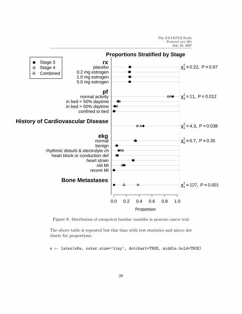
rx 502 χ23 = 0.22, P = 0.971
placebo 26% ( 74) 25% ( 53) 25% (127)0.2 mg estrogen 25% ( 73) 24% ( 51) 25% (124)1.0 mg estrogen 25% ( 71) 26% ( 55) 25% (126)5.0 mg estrogen 25% ( 71) 25% ( 54) 25% (125)
Age in Years 501 70.0 73.0 76.0 (71.8± 6.7) 69.0 73.0 76.0 (71.0± 7.6) 70.0 73.0 76.0 (71.5± 7.1) F1,499 = 0.2, P = 0.662
Weight Index = wt(kg)-ht(cm)+200 500 91 99 109 (100± 13) 89 97 105 ( 97± 14) 90 98 107 ( 99± 13) F1,498 = 5.4, P = 0.0212
pf 502 χ23 = 11, P = 0.0121
normal activity 93% (268) 85% (182) 90% (450)in bed < 50% daytime 6% ( 18) 9% ( 19) 7% ( 37)in bed > 50% daytime 1% ( 3) 5% ( 10) 3% ( 13)confined to bed 0% ( 0) 1% ( 2) 0% ( 2)
History of Cardiovascular Disease 502 46% (134) 37% ( 79) 42% (213) χ21 = 4.3, P = 0.0381
Systolic Blood Pressure/10 502 13.0 14.0 16.0 (14.4± 2.6) 13.0 14.0 16.0 (14.3± 2.2) 13.0 14.0 16.0 (14.4± 2.4) F1,500 = 0.01, P = 0.92
Diastolic Blood Pressure/10 502 7.0 8.0 9.0 (8.2±1.6) 7.0 8.0 9.0 (8.1±1.3) 7.0 8.0 9.0 (8.1±1.5) F1,500 = 0.43, P = 0.512
ekg 494 χ26 = 6.7, P = 0.351
normal 35% ( 98) 33% ( 70) 34% (168)benign 5% ( 14) 4% ( 9) 5% ( 23)rhythmic disturb & electrolyte ch 8% ( 22) 14% ( 29) 10% ( 51)heart block or conduction def 6% ( 17) 4% ( 9) 5% ( 26)heart strain 30% ( 85) 31% ( 65) 30% (150)old MI 17% ( 47) 13% ( 28) 15% ( 75)recent MI 0% ( 1) 0% ( 0) 0% ( 1)
Serum Hemoglobin g/100 ml 502 12.5 13.8 14.9 (13.7± 1.8) 11.8 13.4 14.6 (13.1± 2.1) 12.3 13.7 14.7 (13.4± 2.0) F1,500 = 11, P < 0.0012
Size of Primary Tumor cm2 497 4 8 16 (12±11) 7 17 26 (18±13) 5 11 21 (15±12) F1,495 = 39, P < 0.0012
Combined Index of Stage and Hist. Grade 491 8.0 9.0 9.0 ( 9.1± 1.3) 11.0 12.0 13.0 (12.0± 1.5) 9.0 10.0 11.0 (10.3± 2.0) F1,489 = 605, P < 0.0012
Serum Prostatic Acid Phosphatase 502 0.40 0.50 0.70 ( 0.66± 1.75) 1.60 4.20 20.00 (27.80±93.29) 0.50 0.70 2.97 (12.18±62.17) F1,500 = 802, P < 0.0012
Bone Metastases 502 0% ( 1) 38% ( 81) 16% ( 82) χ21 = 127, P < 0.0011
a b c represent the lower quartile a, the median b, and the upper quartile c for continuous variables. x± s represents X̄ ± 1 SD. N is thenumber of non–missing values. Numbers after percents are frequencies. Tests used: 1Pearson test; 2Wilcoxon test
The EXAMPLE StudyProtocol xyz–001
July 20, 2007
Proportion
0.0 0.2 0.4 0.6 0.8 1.0
●
●
●
●
●
●
●
●
●
●
●
●
●
●
●
●
●
χχ32 == 0.22,, P == 0.97
χχ32 == 11,, P == 0.012
χχ12 == 4.3,, P == 0.038
χχ62 == 6.7,, P == 0.35
χχ12 == 127,, P << 0.001
placebo 0.2 mg estrogen 1.0 mg estrogen 5.0 mg estrogen
normal activity in bed < 50% daytime in bed > 50% daytime
confined to bed
normal benign
rhythmic disturb & electrolyte ch heart block or conduction def
heart strain old MI
recent MI
rx
pf
History of Cardiovascular Disease
ekg
Bone Metastases
●
●
●
●
●
●
●
●
●
●
●
●
●
●
●
●
●
Proportions Stratified by Stage●
●
Stage 3Stage 4Combined
Figure 8: Distribution of categorical baseline variables in prostate cancer trial
The above table is repeated but this time with test statistics and micro dotcharts for proportions.
w ← latex(s6a, outer.size=’tiny’, dotchart=TRUE, middle.bold=TRUE)
39

The EXAMPLE StudyProtocol xyz–001
July 20, 2007
Age in Years55 60 65 70 75 80
[
[
[
Stage 3
Stage 4
Combined
●
●
●
]
]
]
F1,, 499 == 0.2,, P == 0.66
Weight Index = wt(kg)−ht(cm)+20080 90 100 110 120 130
[
[
[
Stage 3
Stage 4
Combined
●
●
●
]
]
]
F1,, 498 == 5.4,, P == 0.021
Systolic Blood Pressure/1010 12 14 16 18 20
[
[
[
Stage 3
Stage 4
Combined
●
●
●
]
]
]
F1,, 500 == 0.01,, P == 0.9
Diastolic Blood Pressure/106 7 8 9 10 11
[
[
[
Stage 3
Stage 4
Combined
●
●
●
]
]
]
F1,, 500 == 0.43,, P == 0.51
Serum Hemoglobin,, g 100ml10 12 14 16
[
[
[
Stage 3
Stage 4
Combined
●
●
●
]
]
]
F1,, 500 == 11,, P << 0.001
Size of Primary Tumor,, cm20 10 20 30 40 50
[
[
[
Stage 3
Stage 4
Combined
●
●
●
]
]
]
F1,, 495 == 39,, P << 0.001
Combined Index of Stage and Hist. Grade6 8 10 12 14
[
[
[
Stage 3
Stage 4
Combined
●
●
●
]
]
]
F1,, 489 == 605,, P << 0.001
Serum Prostatic Acid Phosphatase0 50 100 150 200 250
[
[
[
Stage 3
Stage 4
Combined
●
●
●
]
]
]
F1,, 500 == 802,, P << 0.001
Figure 9: Quartiles of continuous variables in prostate cancer trial. x–axes arescaled to the lowest 0.025 and highest 0.975 quantiles over all groups for eachvariable.
40

The EXAMPLE StudyProtocol xyz–001
July 20, 2007
Table 12: Descriptive Statistics by Stage
N Stage 3 Stage 4 Test StatisticN = 289 N = 213
rx 502 χ23 = 0.22, P = 0.971
placebo 26% (74) 25% (53) 0 1rb0.2 mg estrogen 25% (73) 24% (51) rb1.0 mg estrogen 25% (71) 26% (55) rb5.0 mg estrogen 25% (71) 25% (54) rb
Age in Years 501 70 73 76 69 73 76 F1,499 = 0.2, P = 0.662
Weight Index = wt(kg)-ht(cm)+200 500 91 99 109 89 97 105 F1,498 = 5.4, P = 0.0212
pf 502 χ23 = 11, P = 0.0121
normal activity 93% (268) 85% (182) 0 1rbin bed < 50% daytime 6% ( 18) 9% ( 19) rbin bed > 50% daytime 1% ( 3) 5% ( 10) rbconfined to bed 0% ( 0) 1% ( 2) rb
History of Cardiovascular Disease 502 46% (134) 37% ( 79) χ21 = 4.3, P = 0.0381
Systolic Blood Pressure/10 502 13 14 16 13 14 16 F1,500 = 0.01, P = 0.92
Diastolic Blood Pressure/10 502 7 8 9 7 8 9 F1,500 = 0.43, P = 0.512
ekg 494 χ26 = 6.7, P = 0.351
normal 35% (98) 33% (70) 0 1rbbenign 5% (14) 4% ( 9) rbrhythmic disturb & electrolyte ch 8% (22) 14% (29) r bheart block or conduction def 6% (17) 4% ( 9) rbheart strain 30% (85) 31% (65) rbold MI 17% (47) 13% (28) rbrecent MI 0% ( 1) 0% ( 0) rb
Serum Hemoglobin g/100 ml 502 12 14 15 12 13 15 F1,500 = 11, P < 0.0012
Size of Primary Tumor cm2 497 4 8 16 7 17 26 F1,495 = 39, P < 0.0012
Combined Index of Stage and Hist. Grade 491 8 9 9 11 12 13 F1,489 = 605, P < 0.0012
Serum Prostatic Acid Phosphatase 502 0.4 0.5 0.7 1.6 4.2 20.0 F1,500 = 802, P < 0.0012
Bone Metastases 502 0% ( 1) 38% ( 81) χ21 = 127, P < 0.0011
a b c represent the lower quartile a, the median b, and the upper quartile cfor continuous variables.N is the number of non–missing values.Numbers after percents are frequencies.Tests used: 1Pearson test; 2Wilcoxon test
41

Table 13: mean by sz, bone
Size of Primary Tumor no mets bone mets TotalN ap > 1 N ap > 1 N ap > 1
[0, 6) 128 0.26 7 0.86 135 0.29[6, 12) 109 0.20 16 0.75 125 0.27[12, 22) 97 0.31 19 0.95 116 0.41[22, 69] 81 0.51 40 0.90 121 0.64Missing 5 0.40 0 5 0.40
Total 420 0.30 82 0.88 502 0.40
4.3 Data Displays from Cross–Classifying Variables
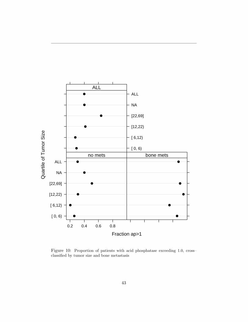
The final examples use cross–classification on possibly more than one in-dependent variable. The summary function with method=’cross’ produces adata frame containing the cross–classifications. This data frame is suitablefor multi-panel trellis displays although if marginal statistics are not needed,the Hmisc summarize function is better. The first example in this series wasLATEX’ed to create Table 13 (the code is listed above).
There is no plot method for method=’cross’ tables, but you can use Trellisgraphics on the data frame that is created by summary (see code above). Forthis purpose, the Hmisc summarize function might be better than summary.formula
for producing the needed aggregated data.
42
Fraction ap>1
Qua
rtile
of T
umor
Siz
e
[ 0, 6)
[ 6,12)
[12,22)
[22,69]
NA
ALL
0.2 0.4 0.6 0.8
●
●
●
●
●
●
no mets
●
●
●
●
●
bone mets[ 0, 6)
[ 6,12)
[12,22)
[22,69]
NA
ALL
●
●
●
●
●
●
ALL
Figure 10: Proportion of patients with acid phosphatase exceeding 1.0, cross–classified by tumor size and bone metastasis
43
5 Handling Special Variables
5.1 Multiple Choice Variables
Clinical reports frequuently must summarize “checklist” or multiple–choicevariables. Such variables are typically listed on a case report form using oneof two methods:
1. Specify up to three primary presenting symptoms:_________ ________ ________Here the respondent writes in up to three symptom codes from a listof perhaps 15 integer codes defined below the question.
2. Check symptoms that are present:headache __ stomach ache __ hangnail __back pain __ neck ache __ wheezing __
When such data are processed, either a series of three categorical variablesor 6 binary variables is created. In what follows we assume that the binaryvariables are coded as numeric 0/1 or as character variables with values(ignoring case) of ’yes’ and ’present’ denoting a positive response. In com-posing a report, we usually want to consider all of these component variablesunder the umbrella of ’Presenting Symptoms’. If using presenting symptomsas stratification (independent) variables, we will want to know an outcomestatistic computed separately for those subjects having headache, those hav-ing stomach ache, etc. These categories will overlap for some subjects. Whensummarizing presenting symptoms stratified by treatment, we will want toknow the proportion of subjects in each treatment group having headache,the proportion having stomach ache, etc., with the proportions summing to> 1.0 if any subject had more than one symptom.
The Hmisc summary.formula function (as well as the describe function) canhandle multiple choice / checklist variables after they are combined into anmChoice variable. An mChoice variable is a character string vector of class’mChoice’ whose elements are integer choice numbers separated by semi-colons. As with factor variables, a levels attribute contains the originalcharacter strings corresponding to the integer 1, 2, . . . . The Hmisc mChoice
function will take as input a series of categorical vector variables (using the
44
first input format above), and make an mChoice variable8. This new objectconsists of values such as ’1;2;9’. The inmChoice function is useful for deter-mining whether a vector of category numbers or labels has all of its elementsturned on in each observation.
Here is an example of the use of mChoice from its help file.
> options(digits=3)> set.seed(3)> n ← 20> sex ← factor(sample(c("m","f"), n, rep=TRUE))> age ← rnorm(n, 50, 5)> treatment ← factor(sample(c("Drug","Placebo"), n, rep=TRUE))
> # Generate a 3-choice variable; each of 3 variables has 5 possible levels> symp ← c(’Headache’,’Stomach Ache’,’Hangnail’,+ ’Muscle Ache’,’Depressed’)> symptom1 ← sample(symp, n, TRUE)> symptom2 ← sample(symp, n, TRUE)> symptom3 ← sample(symp, n, TRUE)> Symptoms ← mChoice(symptom1, symptom2, symptom3, label=’Primary Symptoms’)
> # Note: In this example, some subjects have the same symptom checked> # multiple times; in practice these redundant selections would be NAs> # mChoice will ignore these redundant selections> # If the multiple choices to a single survey question were already> # stored as a series of T/F yes/no present/absent questions we could do:> # Symptoms <- cbind(headache,stomach.ache,hangnail,muscle.ache,depressed)> # where the 5 input variables are all of the same type: 0/1,logical,char.> # These variables cannot be factors in this case as cbind would> # store integer codes instead of character strings.> # To give better column names can use> # cbind(Headache=headache, ’Stomach Ache’=stomach.ache, ...)
> # Following 8 commands only for checking mChoice> data.frame(symptom1,symptom2,symptom3)[1:5,]
8There is also an option to create an entry for ’none’ for subjects for whom no choiceswere selected. The input variables need not have the same levels. A master list of cate-gories is constructed by finding all unique categories in the levels of all variables combined,preserving the order of levels for the factor variables.
45

symptom1 symptom2 symptom31 Muscle Ache Muscle Ache Muscle Ache2 Muscle Ache Muscle Ache Depressed3 Stomach Ache Stomach Ache Depressed4 Headache Muscle Ache Headache5 Depressed Muscle Ache Muscle Ache
> Symptoms[1:5] # Print first 5 subjects’ new mChoice values[1] 1 1;4 2;4 1;3 1;4
> format(Symptoms[1:5])[1] "Muscle Ache" "Muscle Ache;Depressed" "Stomach Ache;Depressed" "Muscle Ache;Headache"[5] "Muscle Ache;Depressed"
> as.numeric(Symptoms[1:5])Muscle Ache Stomach Ache Headache Depressed Hangnail
[1,] 1 0 0 0 0[2,] 1 0 0 1 0[3,] 0 1 0 1 0[4,] 1 0 1 0 0[5,] 1 0 0 1 0
> meanage ← N ← single(5)> for(j in 1:5) {+ meanage[j] ← mean(age[inmChoice(Symptoms,j)])+ N[j] <- sum(inmChoice(Symptoms,j))+ }> names(meanage) ← names(N) <- levels(Symptoms)> meanage
Muscle Ache Stomach Ache Headache Depressed Hangnail48.9 48.4 49.6 49.1 47.1
> NMuscle Ache Stomach Ache Headache Depressed Hangnail
9 12 10 9 7
> # Manually compute mean age for 2 symptoms> mean(age[symptom1==’Headache’ | symptom2==’Headache’ | symptom3==’Headache’])
46
[1] 49.6> mean(age[symptom1==’Hangnail’ | symptom2==’Hangnail’ | symptom3==’Hangnail’])[1] 47.1
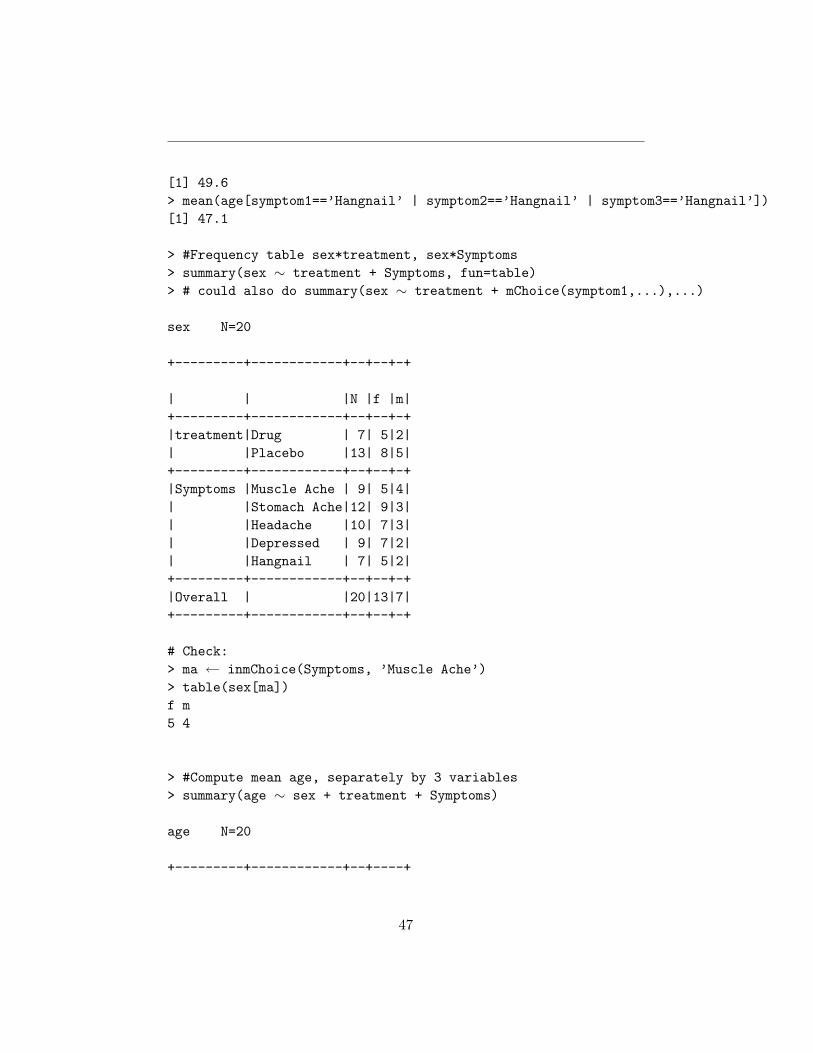
> #Frequency table sex*treatment, sex*Symptoms> summary(sex ∼ treatment + Symptoms, fun=table)> # could also do summary(sex ∼ treatment + mChoice(symptom1,...),...)
sex N=20
+---------+------------+--+--+-+
| | |N |f |m|+---------+------------+--+--+-+|treatment|Drug | 7| 5|2|| |Placebo |13| 8|5|+---------+------------+--+--+-+|Symptoms |Muscle Ache | 9| 5|4|| |Stomach Ache|12| 9|3|| |Headache |10| 7|3|| |Depressed | 9| 7|2|| |Hangnail | 7| 5|2|+---------+------------+--+--+-+|Overall | |20|13|7|+---------+------------+--+--+-+
# Check:> ma ← inmChoice(Symptoms, ’Muscle Ache’)> table(sex[ma])f m5 4
> #Compute mean age, separately by 3 variables> summary(age ∼ sex + treatment + Symptoms)
age N=20
+---------+------------+--+----+
47
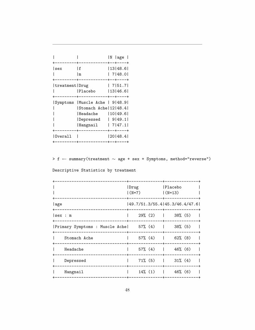
| | |N |age |+---------+------------+--+----+|sex |f |13|48.6|| |m | 7|48.0|+---------+------------+--+----+|treatment|Drug | 7|51.7|| |Placebo |13|46.6|+---------+------------+--+----+|Symptoms |Muscle Ache | 9|48.9|| |Stomach Ache|12|48.4|| |Headache |10|49.6|| |Depressed | 9|49.1|| |Hangnail | 7|47.1|+---------+------------+--+----+|Overall | |20|48.4|+---------+------------+--+----+
> f ← summary(treatment ∼ age + sex + Symptoms, method="reverse")
Descriptive Statistics by treatment
+------------------------------+--------------+--------------+| |Drug |Placebo || |(N=7) |(N=13) |+------------------------------+--------------+--------------+|age |49.7/51.3/55.4|45.3/46.4/47.6|+------------------------------+--------------+--------------+|sex : m | 29% (2) | 38% (5) |+------------------------------+--------------+--------------+|Primary Symptoms : Muscle Ache| 57% (4) | 38% (5) |+------------------------------+--------------+--------------+| Stomach Ache | 57% (4) | 62% (8) |+------------------------------+--------------+--------------+| Headache | 57% (4) | 46% (6) |+------------------------------+--------------+--------------+| Depressed | 71% (5) | 31% (4) |+------------------------------+--------------+--------------+| Hangnail | 14% (1) | 46% (6) |+------------------------------+--------------+--------------+
48

5.2 Conditionally Defined Variables
Another type of variable that is common in clinical reports is a variable thatis of no interest unless another variable equalled a certain value. A commonexample is cause of death. We may want our report to contain the proportionof patients dying on each treatment, and for the deaths, we may want toknow the proportions of deaths due to each cause. For the latter calculation,the denominator is not the number of subjects in a treatment but rather thenumber of subjects who died on that treatment. summary.formula will handlesuch variables correctly as long as they have missing values when they arenot pertinent. For example, suppose that the variable death.cause is NA ifdeath is F (false) and death.cause is a categorical (or mChoice) variable if death
is T. Then a ’reverse’ type summary will produce the needed proportions ofdeath as well as death.cause.
6 Alternate Approaches
6.1 Literate Programming
In literate programming as used in reproducible research (see biostat.mc.vanderbilt.edu/StatReport), a single source document contains analy-sis code as well as text for the report. This has been found to be easier tomaintain and to result in better documentation. Under R, the Sweave packageprovides a concise syntax for mixing S and LATEX code for producing reports,as discussed in Section 16.3 of the course notes at biostat.mc.vanderbilt.edu/StatCompCourse. Sweave will run the S code chunks through R, includeS printed output in the report, and will generate LATEX commands to au-tomatically include graphics generated by the S code. One especially nicefeature of Sweave is the ease with which users can insert variables computedby S into LATEX text without the need of the \def\varname{value} ap-proach described earlier.
Sweave is particularly well suited for non-recurring statistical reports. Re-ports that are run after periodic data updates, for which the time spentpolishing the report is well spent, are sometimes better suited to the cus-tomized programming methods described earlier in this document.
49

7 Data Preparation
For making nice–looking tables, as well as for having self–documenting vari-ables, it is important to spend time defining good variable and value labels.If you are managing the data in SAS, for example, specify nice variable la-bels in a DATA step or using PROC DATASETS, and specify pretty valuelabels using PROC FORMAT. Both variable and value labels should useletter cases carefully. Don’t use all upper case for either kinds of labels.Variable labels should often contain units of measurements. An example ofa good label is ’Serum Cholesterol, mg/dl’. Better still, separate the ’units’
attribute from the ’label’ attribute of a variable:
label(chol) ← ’Serum Cholesterol’units(chol) ← ’mg/dl’# Alternate approach:mydata ← upData(mydata, labels=c(chol=’Serum Cholesterol’),
units =c(chol=’mg/dl’))
Some of the latex and plot methods in the Hmisc and Design libraries makespecial use of units attributes by typesetting them in a different font or byright-justifying units in cells of LATEX tables.
Binary variables are often coded 0/1. Good variable labels for these are ofthe form ’Nocturnal angina present’. Sometimes you may want printouts tobe more self–documenting. Then consider defining a SAS format of the form0=’Angina absent’ 1=’Angina present’.
You can always change labels and value labels after data are imported intoS. Here are some examples.
label(age) ← ’Age (y)’levels(pain) ← c(’None’,’Mild’,’Moderate’,’Severe’)levels(pain) ← list(’Moderate/Severe’=c(’Moderate’,’Severe’))#Combines last two levels for subgroup analyses in which#there were two few patients with severe pain
levels(symptom)[3] ← ’Night sweats’ # fix one level
#Give fuller labels to levels of a binary variable
50
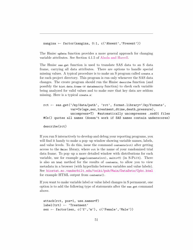
nangina ← factor(nangina, 0:1, c(’Absent’,’Present’))
The Hmisc upData function provides a more general approach for changingvariable attributes. See Section 4.1.5 of Alzola and Harrell.
The Hmisc sas.get function is used to translate SAS data to an S dataframe, carrying all data attributes. There are options to handle specialmissing values. A typical procedure is to make an S program called create.s
for each project directory. This program is run only whenever the SAS datachanges. The create program should run the Hmisc describe function (andpossibly the hist.data.frame or datadensity function) to check each variablebeing analyzed for valid values and to make sure that key data are seldommissing. Here is a typical create.s:
rct ← sas.get(’/my/data/path’, ’rct’, format.library=’/my/formats’,var=Cs(age,sex,treatment,dtime,death,pressure),uncompress=T) #automatically uncompresses .ssd01 files
#Cs() quotes all names (doesn’t work if SAS names contain underscores)
describe(rct)
If you run S interactively to develop and debug your reporting programs, youwill find it handy to make a pop–up window showing variable names, labels,and value levels. To do this, issue the command contents(rct) after gettingaccess to the Hmisc library, where rct is the name of your randomized trialdata frame. To pop–up a more detailed window with distributions for eachvariable, use for example page(contents(rct), multi=T) (in S-Plus). Thereis also an html method for the results of contents, to allow you to viewmetadata in a browser (with hyperlinks between variables and value labels).See biostat.mc.vanderbilt.edu/twiki/pub/Main/DataSets/Cpbc.htmlfor example HTML output from contents().
If you want to make variable label or value label changes in S permanent, oneoption is to add the following type of statements after the sas.get commandabove.
attach(rct, pos=1, use.names=F)label(trt) ← ’Treatment’sex ← factor(sex, c(’f’,’m’), c(’Female’,’Male’))
51
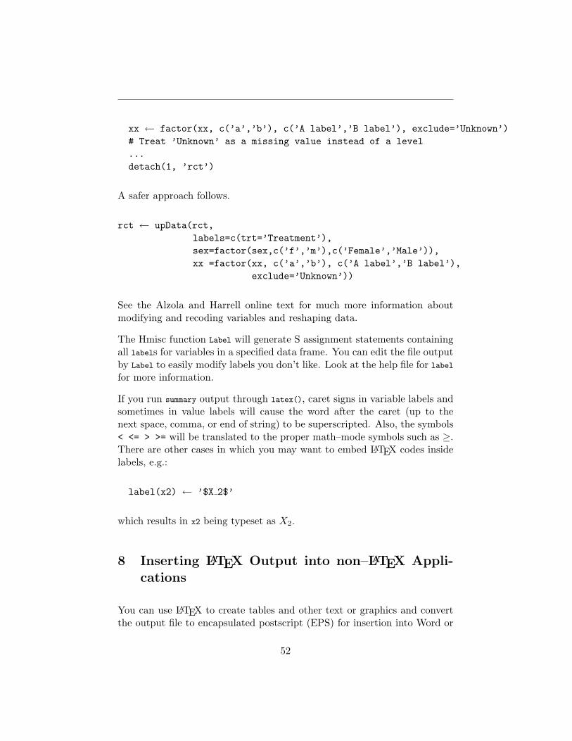
xx ← factor(xx, c(’a’,’b’), c(’A label’,’B label’), exclude=’Unknown’)# Treat ’Unknown’ as a missing value instead of a level...detach(1, ’rct’)
A safer approach follows.
rct ← upData(rct,labels=c(trt=’Treatment’),sex=factor(sex,c(’f’,’m’),c(’Female’,’Male’)),xx =factor(xx, c(’a’,’b’), c(’A label’,’B label’),
exclude=’Unknown’))
See the Alzola and Harrell online text for much more information aboutmodifying and recoding variables and reshaping data.
The Hmisc function Label will generate S assignment statements containingall labels for variables in a specified data frame. You can edit the file outputby Label to easily modify labels you don’t like. Look at the help file for label
for more information.
If you run summary output through latex(), caret signs in variable labels andsometimes in value labels will cause the word after the caret (up to thenext space, comma, or end of string) to be superscripted. Also, the symbols< <= > >= will be translated to the proper math–mode symbols such as ≥.There are other cases in which you may want to embed LATEX codes insidelabels, e.g.:
label(x2) ← ’$X 2$’
which results in x2 being typeset as X2.
8 Inserting LATEX Output into non–LATEX Appli-cations
You can use LATEX to create tables and other text or graphics and convertthe output file to encapsulated postscript (EPS) for insertion into Word or
52
Wordperfect “pictures”. These pictures will not be viewable on the screen(a blank box with be displayed) but they will print correctly as long asyou remember to set your printer to a postscript printer before actuallyprinting. Once you import the picture you can re–size it (if you use a 300dpi postscript driver, making the image larger will result in fuzzy printing).
Use the dvips program to make an EPS file from a LATEX dvi file, using theE option. Here is an example for the simple case in which the document isonly one page long (e.g., it consists of a single table).
dvips -E -o doc.eps doc # creates doc.eps from doc.dvi
If you have a multiple–page LATEX document, you can tell dvips which pageto store in a separate EPS file, for example, page 9:
dvips -E -p 9 -l 9 -o nine.eps doc
You can even have dvips put every page of the document into a separate file.The files will be numbered e.g. doc.001, doc.002, doc.003, ...:
dvips -E -S 1 -i -o doc.0 doc
In Linux an easy way to extract a particular page from a pdf document isto use xpdf or kpdf and print that page to pdf. Then it can be inserted as apicture.
Note that S plots can be output directly as encapsulated postscript or pdf,so you can include them in any document with no extra steps, as long as youstored only one plot in the file. A nice way to pick out individual postscriptplots and store them in a separate .ps file is to use a postscript utilityprogram called psselect, e.g. if you created 3 pages of plots in myplots.ps use
psselect -p1 myplots.ps myplots1.ps
to put the first page of myplots.ps into myplots1.ps. psselect can also be usedto split out desired pages from a postscripted version of a LATEX document asan alternative to using the page number or section splitting options to dvips.Michael Stevens of Duke University has written a program called oneperpg
53

which will go through a multiple–page postscript file and automatically cre-ate separate files each containing one page of output, using psselect. Forexample, typing
oneperpg myplots
creates myplots1.ps, myplots2.ps, myplots3.ps.
Other ways to convert LATEX output to other formats are described at http://biostat.mc.vanderbilt.edu/SweaveConvert. As described there, TeX4htcan convert extremely complex summary.formula LATEX tables (including thosecontaining micro dot charts) to HTML. The resulting HTML file may beopened in OpenOffice and exported to an open document file, which canbe opened and saved in Microsoft Word format. If the document containspictures (e.g., micro dot charts), embed the pictures in the document afterexporting it to open document format, by clicking on the OpenOffice Edit
and Links menus, highlighting all picture file names using shift-left-click,and clicking Break Link. An OpenOffice version of table 12 may be viewed athttp://biostat.mc.vanderbilt.edu/twiki/pub/Main/StatReport/s6a.odt.
You can insert the HTML file into Microsoft Word 97 documents, but if yousave the document as a Word file rather than as HTML, special formattingsuch as LATEX font size changes will be lost. This is because Microsoftis not consistent in how enhanced HTML commands are implemented inInternet Explorer and in Word9. In addition to this problem, latex2html
does not convert all table commands properly; sometimes the program juststops in the middle of the conversion. If you have any math commands inthe document, latex2html has to convert these to GIF images. latex2html isobsolete given TeX4ht.
In general, HeVeA (http://pauillac.inria.fr/∼maranget/hevea/) doesan excellent job in converting simpler LATEX code to HTML, without theneed for graphics images for math commands. For some applications theresulting HTML can easily be inserted into Word documents.
9I have not tested this under newer versions of Word.
54

9 S Documention
Use the command ?summary.formula under S to get detailed document ofsummary.formula and its print, plot, and latex methods.
10 LATEX Code for This Document
% Usage: pdflatex --shell-escape summary --shell-escape enables sinput
\documentclass[11pt]{article}
% Style Purpose% ------------ -------------------------------------------------% graphicx LaTeX graphics package with rotation etc.% ctable Nice tables with bolder initial horizontal line% moreverb Inclusion of text files (verbatimtabinput)% fancyhdr Headers, footers (rhead)% lscape Landscape model (landscape)% sinput Inclusion of S code with automatic reformatting% hyperref Hyper--referencing for electronic documents (pdf)% url Split long URLs (part of hyperref)% relsize Specify font sizes as relative to current normalsize% calc, epic, color Used for micro dot charts inside tables\usepackage{graphicx}\usepackage{ctable}\usepackage{moreverb}\usepackage{fancyhdr}\usepackage[pdftex]{lscape}\usepackage{sinput}\usepackage{relsize}\usepackage{calc,epic,color}
\newcommand{\splus}{{S-P\sc{lus}}}\newcommand{\R}{{\normalfont\textsf{R}}{}}\newcommand{\scom}[1]{{\rm\scriptsize \# #1}}% defines how sinput prints S comments\newcommand{\code}[1]{\texttt{\smaller #1}} % format software names% smaller implemented by relsize: use 1 size smaller than current font
%\newcommand{\titl}{Statistical Tables and Plots using S and LaTeX}\usepackage[pdftex,bookmarks,pagebackref,colorlinks,pdfpagemode=UseOutlines,
55

pdfauthor={Frank E Harrell Jr},pdftitle={Statistical Tables and Plots using S and LaTeX}]{hyperref}
% Macros to start and end in-line S code listings (assumes sinput in effect)\newcommand{\bex}{\begin{list}{}{\setlength{\leftmargin}{\parindent}}%\item%\begin{alltt}%}\newcommand{\eex}{\end{alltt}%\end{list}%}
% The following macro makes insertion of pdf figures easy.% Usage: \fig{label=.pdf prefix}{caption}{short caption for list of% figures}{scalefactor}\newcommand{\fig}[4]{\begin{figure}[hbp!]\leavevmode\centerline{\includegraphics[scale=#4]{#1.pdf}}\caption[#3]{\small #2}\label{#1}\end{figure}}
% The following macro makes insertion of pdf figures easy. Unfortunately,% inserting .pdf figures results in wasted space before and after the% graph. This can be fixed by providing vspace commands with negative% heights.%\pdfig{label=.pdf prefix}{caption}{short caption}{scalefactor}{leftshift}%{vspace before figure (try -2in)}{vspace before caption(try -2in)}\newcommand{\pdfig}[7]{\begin{figure}[htbp]\begin{center}
\vspace{#6}\scalebox{#4}{\hspace{#5}\includegraphics{#1.pdf}}\vspace{#7}\caption[#3]{\small #2}\label{#1}\end{center}\end{figure}}
\setlength{\parindent}{0ex} % don’t indent first line of paragraph\setlength{\parskip}{2ex} % do skip 2 spaces between paragraphs
\pagestyle{fancy} % used for running headers, footers (rhead)\renewcommand{\subsectionmark}[1]{} % suppress subsection titles in headers
\begin{document}
56
\title{Statistical Tables and Plots using S and \LaTeX}
\author{FE Harrell \\Department of Biostatistics \\Vanderbilt University School of Medicine \\
\href{mailto:[email protected]}{\url{[email protected]}} \\ ~ \\\href{http://biostat.mc.vanderbilt.edu}{\url{biostat.mc.vanderbilt.edu}}\footnote{Document Address:\href{http://biostat.mc.vanderbilt.edu/twiki/pub/Main/StatReport/summary.pdf}{\url{http://biostat.mc.vanderbilt.edu/twiki/pub/Main/StatReport/summary.pdf}}. Thisdocument was produced using Te\TeX\ on Ubuntu Linux using \R\version 2.5.1 and version 3.3-3 (17Jul07) of the \code{Hmisc}package. All commands and output will be the same for \splus\ exceptthat Greek letters, superscripts, and subscripts will not appear inplots.}}\date{\today}\maketitle
\tableofcontents\listoftables\listoffigures
\section{Introduction to \LaTeX}\LaTeX\ is a public domain document processing system developed byLamport (which uses \TeX\ by Knuth) that is used heavily in thesciences and by journal and book publishers\footnote{\LaTeX\ isavailable on many platforms. An excellent free versions for MicrosoftWindows is Mik\TeX, both available at\href{http://www.ctan.org}{\url{www.ctan.org}}.An excellent free book on \LaTeX\ is available at\href{http://ctan.tug.org/tex-archive/info/lshort/english/lshort.pdf}{\url{ctan.tug.org/tex-archive/info/lshort/english/lshort.pdf}}}.\LaTeX\ is a {\em markup language} that is compiled similar toprogramming languages such as C. \LaTeX\ is particularly strong inlayouts, cross--referencing, typesetting equations, making tables,bibliographic citations, indexes and tables of contents, and allowingfor insertion of graphics in documents. This makes \LaTeX\ verysuitable for compiling long statistical reports such as those used tosupport drug licensing. For this purpose, major advantages of \LaTeX\include the ability to automatically create cross--references and toautomatically update a report if any of its component graphics figuresor tables changes. To accomplish the latter capability, the analystmerely re--runs the statistical program that produced the graphics or
57

table components. These graphics and tables are read respectively by\LaTeX\ by an \verb|\includegraphics{}| or \verb|\input{}| command, sorunning the \code{latex} command to recompile to report will make anyneeded updates. This is in distinction to Microsoft Word, which doesnot have a batch inclusion capability.
Everything in a \LaTeX\ source document is plain text, soyou can edit these documents using any text editor\footnote{The\code{Emacs} editor has a special mode for editing \LaTeX\ text thatmakes composing text much easier.} and E--mail them to
anyone. \LaTeX\ is based on the philosophy that the writer should havean easy time composing and editing text\footnote{For example, with one\code{Emacs} command you can change the first word of every figurecaption to be in another font, or change the size of all includedfigures.} but she should not have to spend time making text look
good on the screen. Instead the writer needs to concentrate on thelogical elements of composition; \LaTeX’s job is to make the finaloutput look good.
\subsection{Two \LaTeX\ Output Modes}When the \code{latex} command is run to compile your \LaTeX\ sourcecode, \LaTeX\ produces a dvi (‘‘device independent’’) file containingthe typeset document in a very compact form. Graphics are notincluded in the dvi file, but pointers to the graphics files areincluded. The dvi file can be printed directly, or it can beconverted into a self--contained postscript or pdf file. Here aresome example \LaTeX-related system commands.\begin{verbatim}latex myfile % create myfile.dvi from myfile.texdvips myfile % send myfile to a postscript printerdvips -o myfile.ps myfile % convert myfile.dvi to myfile.ps, with
% graphicsdvips -Pwww -o myfile.ps myfile % use Type 1 fontsdvipdfm myfile % convert myfile.dvi to myfile.pdfpdflatex myfile % creates myfile.pdf directly if no
% postscript graphics are referenced\end{verbatim}
Creation of a static document in one of these ways is the usual modeof \LaTeX\ usage. There is also a way of using \LaTeX\ to create‘‘live’’ documents that are viewed on a monitor (either locally orover the web) or printed. These pdf documents may contain bookmarks,hyperlinks to external URLs, links to E--mail addresses, etc. If youuse the \code{hyperref} package in \LaTeX, the system willautomatically make all pertinent elements of your document
58

cross--indexed and hyperlinked, and you can also insert specialcommands to link to areas outside the document such as URLs andE--mail.
When viewing the document using Adobe Acrobat Reader, bookmarks canappear in the left margin, allowing the user to click to jump to anymajor section of the document. Sections having sub--sections can havetheir bookmarks expanded so that you can jump to the sub--sections.You can jump to any figure while viewing the \code{List of Figures} andto any table while viewing the \code{List of Tables}, in addition tojumping to any area while viewing the \code{Table of Contents}. Ifyour document is indexed, you can jump to any page for which anindexed phrase is discussed. You can optionally jump to pages inwhich a given article is cited while viewing the \code{Bibliography},in addition to the more standard jump from a citation to thebibliographic reference. If the \code{colorlinks} option is selected(see code below), symbols that are hyperlinked appear in color;clicking on them will cause the jump. All of this is set upautomatically by \code{hyperref}, unlike the large number of flags thatmust be put in a document manually if using Microsoft Word.
Instead of compiling the document using the \code{latex} systemcommand, you use the \code{pdflatex} command to create the pdf filedirectly, with all bookmarks and hyperlinks.
This document was created in the fashion just described. \code{PDF}graphics files were created directly using an S \code{pdf} devicedriver. Below you will find the code in the preamble of the documentthat set up the \code{pdf} document with hyper--referencing.\begin{verbatim}\usepackage[pdftex,bookmarks,pagebackref,colorlinks,pdfpagemode=UseOutlines,
pdfauthor={Frank E Harrell Jr},pdftitle={Statistical Tables and Plots using S and LaTeX}]{hyperref}
\end{verbatim}
\subsection{Basic Table Making in \LaTeX}\LaTeX\ has excellent facilities for composing and typesetting tables.Table \ref{results} is an example of a user--specified table usingthree macros --- \code{btable} (begin table), \code{etable} (end table),and \code{mc} (headings that span multiple columns). These macros saverepetitive operations. Macros are usually defined at the top ofthe document.\begin{verbatim}%Usage: \btable{table specs}{caption}{reference label}\newcommand{\btable}[3]{
59

\begin{table}[htbp]\begin{center}\caption{#2\label{#3}}\begin{tabular}{#1}}
\newcommand{\etable}{\end{tabular}\end{center}\end{table}}
%Usage: \mc{number of columns spanned}{major column heading}\newcommand{\mc}[2]{\multicolumn{#1}{c}{#2}}
\btable{l|ccccc}{Overall Results}{results} \hline\hline%6 fields, justified left, center x 5%double horizontal line at top, 1 vertical bar& \mc{2}{Females} & & \mc{2}{Males} \\ % column 4 blank, for spacing\cline{2-3} \cline{5-6} % horizontal lines connecting cols. 2-3, 5-6Treatment & Mortality & Mean Pressure & & Mortality & Mean Pressure \\ \hlinePlacebo & 0.21 & 163 & & 0.22 & 164 \\ACE Inhibitor & 0.13 & 142 & & 0.15 & 144 \\Hydralazine & 0.17 & 143 & & 0.16 & 140 \\ \hline\etable\end{verbatim}
%Usage: \btable{table specs}{caption}{reference label}\newcommand{\btable}[3]{
\begin{table}[htbp]\begin{center}\caption{#2\label{#3}}\begin{tabular}{#1}}
\newcommand{\etable}{\end{tabular}\end{center}\end{table}}
%Usage: \mc{number of columns spanned}{major column heading}\newcommand{\mc}[2]{\multicolumn{#1}{c}{#2}}
\btable{l|ccccc}{Overall Results}{results} \hline\hline%6 fields, justified left, center x 5%double horizontal line at top, 1 vertical bar& \mc{2}{Females} & & \mc{2}{Males} \\ % column 4 blank, for spacing\cline{2-3} \cline{5-6} % horizontal lines connecting cols. 2-3, 5-6Treatment & Mortality & Mean Pressure & & Mortality & Mean Pressure \\ \hlinePlacebo & 0.21 & 163 & & 0.22 & 164 \\
60

ACE Inhibitor & 0.13 & 142 & & 0.15 & 144 \\Hydralazine & 0.17 & 143 & & 0.16 & 140 \\ \hline\etableThe result is Table~\ref{results}.However, the \texttt{ctable} style, available from\href{http://www.ctan.org}{\url{www.ctan.org}} can produce prettier tablesmore flexibly:\begin{verbatim}\ctable[caption={Overall Results},label=resultsb,pos=hbp!]{lccccc}{}{\FL& \mc{2}{Females} & & \mc{2}{Males} \NN\cmidrule{2-3}\cmidrule{5-6} % Important: no space before \cmidruleTreatment & Mortality & Mean Pressure & & Mortality & Mean Pressure \MLPlacebo & 0.21 & 163 & & 0.22 & 164 \NNACE Inhibitor & 0.13 & 142 & & 0.15 & 144 \NNHydralazine & 0.17 & 143 & & 0.16 & 140 \LL}\end{verbatim}The result is shown in Table~\ref{resultsb}.\ctable[caption={Overall Results},label=resultsb,pos=hbp!]{lccccc}{}{\FL& \mc{2}{Females} & & \mc{2}{Males} \NN\cmidrule{2-3}\cmidrule{5-6}Treatment & Mortality & Mean Pressure & & Mortality & Mean Pressure \MLPlacebo & 0.21 & 163 & & 0.22 & 164 \NNACE Inhibitor & 0.13 & 142 & & 0.15 & 144 \NNHydralazine & 0.17 & 143 & & 0.16 & 140 \LL}
\section{Using S to Fill in Cells in \LaTeX\ Tables}For most statistical tables a better idea is to avoid transcription ofcalculated values by having the values inserted into tablesautomatically. The \texttt{Hmisc} library (see\href{http://biostat.mc.vanderbilt.edu/Hmisc}{\url{biostat.mc.vanderbilt.edu/Hmisc}})contains several S functions by R Heiberger and F Harrell thatautomatically make \LaTeX\ tables fromS objects\footnote{More advanced applications of this are foundin the \code{Design} library, such as automatic \LaTeX\ typesetting offitted regression models with simplification of interaction and splineterms, and typesetting of $\chi^2$ tables showing all regressioneffects. These examples are beyond the scope of this document. See\href{http://biostat.mc.vanderbilt.edu/twiki/pub/Main/RS/sintro.pdf}{\url{biostat.mc.vanderbilt.edu/twiki/pub/Main/RS/sintro.pdf}}, Chapter 9.}.S functions that automatically produce \LaTeX\ code from S
61

objects (matrices, fitted models, data summaries, etc.) have namesthat start with \code{latex}. Tables produced by the \code{latex.*}functions in \code{Hmisc} meet the stylistic requirements ofmost journals, i.e., by default they do not use vertical lines andthey use horizontal lines only when needed. In this way the lines donot distract from delivering the statistical information.
Suppose that some calculations have already been made using S,and these calculations were not stored. For example, you may haveestimated various effects and standard errors but forgot to store theS regression fit objects so that you can pull these values intotables automatically. You can use the \code{latex.default} functionthat is part of \code{Hmisc} for automatic conversion of thecalculations into \LaTeX, after entering basic statistics manually.Let us have S calculate odds ratios and $P$--values to avoidtranscribing them after we print $\hat{\beta}$ and standard errors.Here is the S program for creating the table that is insertedinto this document as Table \ref{summary.stats}.\sinput{summary.stats.s}\input{summary.stats}
There are many other options to the basic \code{latex} function. Type\code{?latex} to access the online help. You may be particularlyinterested in the \code{longtable} option, which can be used to easilybreak a long table into multiple pages (with repetitions of key headerinformation).
You can have your S program print hardcopy \LaTeX\ outputdirectly using the \code{prlatex} function. More typically though youwill want the program to create \LaTeX\ files (with suffix \code{.tex})that will be put together later. In this way you can add title pages,running headers or footers, and other text, and refer to tables bysymbolic names. This document serves as an example of how this isdone, with its \LaTeX\ code listed in Section \ref{latex.code}.
If you like to specify table layouts inside the \LaTeX\ source filerather than inside S, you can have your S program outputsymbolic values to a file that is \verb|\input{}|’d in \LaTeX\ asshown in the following example. A restriction is that variable namesdefined to \LaTeX\ may contain only letters and they should notcoincide with names of \LaTeX\ commands.\begin{verbatim}chisq <- (beta/se)^2pval <- 1 - pchisq(chisq, 1)cat(’\\def\\chisq{’,round(chisq,2),’}\\n’, # \\ -> \ in parms.tex
62
’\\def\\pval{’,round(pval,4),’}\n’, sep=’’, file=’parms.tex’)\end{verbatim}If \LaTeX\ variables are named the same as S variables, andthe names contain only letters, code can be simplified using a littlefunction. This function can also convert \code{NA}s to blanks.\begin{verbatim}lvar <- function(x, digits=2)paste(’\\def\\’,substitute(x),’{’,
ifelse(is.na(x),’’,round(x,digits)),’}’, sep=’’)
cat(lvar(chisq), lvar(pval,4), sep=’\n’, file=’parms.tex’)\end{verbatim}
The contents of file \code{parms.tex} will look like the following:\begin{verbatim}\def\chisq{3.84}\def\pval{0.05}\end{verbatim}Inside the main \LaTeX\ source file use for example\begin{verbatim}\input{parms}\ctable[caption={Main Results},label=resultsc]{lcc}{}{Test & $\chi^2$ & $P$--value \MLAge effect & \chisq & \pval \LL}\end{verbatim}
\section{Using S to Create Graphics for \LaTeX}PostScript is a graphics format accepted by all versions of \LaTeX\ aslong as you have a PostScript printer or have GhostScript or AdobeAcrobat Distiller to convert postscript output to other formats. Thebasic graphics driver in S for creating postscript files is the\code{postscript} function. For creating 35mm slides, overheadtransparencies, or $5 \times 7$ glossy figures, the \code{ps.slide}function in the Hmisc library assists in setting up nice defaults forpostscript images. For reports and books, the Hmisc \code{setps}function makes creating of individual postscript graphicseasy\footnote{The corresponding Hmisc function for creating pdf filesis \code{setpdf}. You can also use the \code{postscript} and\code{pdf} functions directly. Some useful templates for doing somay be found at\url{http://biostat.mc.vanderbilt.edu/SgraphicsHints}.}.
\code{setps} uses reasonable defaults and sets up for a minimally sizedbounding box. It tries not to waste space between axes and axislabels. In the following example, a file called \code{test.ps} is
63

created in the current working directory. Note the absence of quotemarks around the word \code{test} below.\bexsetps(test) \scom{use setps(test, trellis=T) if using Trellis (R Lattice)}plot(....)dev.off() \scom{close file, creating test.ps}\eexAs you will see later, we can symbolically label this figure using theword \code{test} in \LaTeX. By default, \code{setps} uses Helveticafont and makes small book--style figures. There are many options tooverride these and other settings.
If you are using \code{pdflatex}, graphics files must be in Adobe \code{pdf}format. You can create \code{pdf} files directly in\splus\ using the builtin \code{pdf.graph} function, in \R\ using the\code{pdf} function, or using the Hmisc \code{setpdf} function. Inolder versions of \splus, better results are obtained by creatingpostscript and converting the graph to \code{pdf}. If you haveGhostscript installed and have used \code{setps} followed by\code{dev.off}, you can type \code{topdf()} with no arguments to invokeGhostscript from S to create, in this case, \code{test.pdf}. Youcan also convert from postscript to \code{pdf} using Adobe AcrobatDistiller, which produces more compact \code{pdf} files. In \R, directcreation of \code{.pdf} files seems to work well.
\subsection{Inserting Graphics Files into \LaTeX\ Documents}The standard \code{graphics} and \code{graphicx} packages in \LaTeX\provide all you need to insert postscript and \code{pdf} graphics into adocument in a flexible fashion. This is not to say that it is as easyas using Word; frequently some trial and error is required to getgraphics tohave an appropriate scaling (magnification) factor. Inclusion of \code{pdf}graphics in older versions of \splus\ and \LaTeX\ frequently resultedin much wasted spaced before and after thegraph when using \code{pdflatex}, so you often had to use\verb|\vspace| commands with negative arguments when including \code{pdf}files.
Here is a \LaTeX\ macro for inserting \code{pdf} graphics files, which are assumed tohave a \texttt{.pdf} suffix.\begin{verbatim}% Usage: \fig{label=.pdf prefix}{caption}{short caption for list of% figures}{scalefactor}\newcommand{\fig}[4]{\begin{figure}[hbp!]\leavevmode\centerline{\includegraphics[scale=#4]{#1.pdf}}
64
\caption[#3]{\small #2}\label{#1}\end{figure}}\end{verbatim}For example, \verb|\fig{test}{long caption}{short caption}{.8}|will insert \code{test.pdf} and reduce its size by $20\%$. You canrefer to this figure in the text using for example\verb|see Figure~\ref{test}|.
\section{Making S Compose \LaTeX\ Tables}In many cases S functions can be used to make all calculationsfor the table and then to create the \LaTeX\ table. Harrell’s S\\code{summary} function for formulas (actually \code{summary.formula})is one function that will do this when what you need is descriptivestatistics (including statistics computed by functions you create).\code{summary} is in the Hmisc library available at\href{http://biostat.mc.vanderbilt.edu/Hmisc}{\url{biostat.mc.vanderbilt.edu/Hmisc}}.It has three methods forcomputing descriptive statistics on univariate or multivariateresponses, subsetted by categories of other variables. See {\em AnIntroduction to S and the Hmisc and Design Libraries} by CFAlzola and FE Harrell(\href{http://biostat.mc.vanderbilt.edu/twiki/pub/Main/RS/sintro.pdf}{\url{biostat.mc.vanderbilt.edu/twiki/pub/Main/RS/sintro.pdf}}) formore information about \code{summary.formula} and S usage ingeneral, especially information on how to recode and reshape data tobe used in reports.
The output from \code{summary.formula} can be printed (for ordinarytext file printouts), plotted (dot charts or occasionallybox-percentile plots), or typeset using \LaTeX,as there are several \code{print}, \code{plot}, and \code{latex} methodsfor objects created by \code{summary.formula}. The \code{latex} methodscreate all the needed table elements, then invoke the\code{latex.default} method in \code{Hmisc} to build the complete set of\LaTeX\ commands to make each table.
The method of data summarization to be done by \code{summary.formula}is specified in the parameter \code{method}. These methods are definedbelow. For the first and third methods, the statistics used tosummarize the data may be specified in a flexible manner by the user(e.g., the geometric mean, $33^{rd}$ percentile, or Kaplan--Meier2--year survival estimate, mixtures of several statistics). Thedefault summary statistic is the mean, which for a binary response
65
variable is the proportion of positive responses.
\begin{description}\item[\code{method=’response’}:\ ] The response variable may bemultivariate, and any number of statistics may be used to summarizethe responses. Sometimes dependent variables are multivariatebecause they indicate follow--up time and censoring, and sometimesthey are multivariate because there are several response variables(e.g., systolic and diastolic blood pressure). The responses aresummarized separately for each independent variable (independentvariables are not cross--classified). Continuous independentvariables are automatically stratified into quantile groups. One ormore of the independent variables may be stratification factors, inwhich all computations are done separately by levels of thesecategorical variables. The stratification variables form majorcolumn groupings in tables. For multivariate responses, subjects areconsidered to be missing if {\em any} response variable is missing.\item[\code{method=’reverse’}:\ ]This format is typical of baseline characteristic tables describingthe usual success of randomization. Here the single dependentvariable must be categorical (e.g., treatment assignment), and the‘‘independent’’ variables are broken down separately by the dependentvariable. Continuous independent variables are described by threequantiles (quartiles by default), and categorical ones are describedby counts and percentages. There is an option to automaticallygenerate test statistics for testing across columns of\code{’reverse’} tables.\item[\code{method=’cross’}:\ ]The \code{’cross’} method allows allows for multiple dependentvariables and multiple statistics to summarize each one. If there ismore than one independent variable (up to three is allowed),statistics are computed separately for all cross--classifications ofthe independent variables, and marginal and overall statistics mayoptionally be computed. \code{summary.formula} for this methodoutputs a data frame containing the combinations of predictors alongwith the response summaries. This data frame may be summarizedgraphically in various ways using the \splus\ \code{trellis}library or \R\ \code{lattice} package\footnote{For this purpose, theHmisc \code{summarize} functionmay be more useful, if you don’t want marginal statistics computed.}.A \LaTeX\ printing method, for the case where there is exactly twopredictors, typesets a two--way table where the first predictor formsrows and the second forms columns. Like \code{method=’response’}, continuousvariables are automatically divided into quantile groups.\end{description}
66
The \code{latex} methods in the \code{Hmisc} librarycreate tables using standard \LaTeX\ commands. These tables areinserted into the master document at the desired location using an\verb|\input{}| command. \code{latex} methods allow a font \code{size}argument. For example, you may specify \code{size=’small’} to\code{latex()}, or you may want to use a generic size that is set at\LaTeX\ run time in the document preamble. For example,specify \verb|\def\tsz{small}| in the master document andspecify \code{size=’tsz’} to \code{latex()}. Then you can define (andredefine) the size for tables without modifying the individual\code{.tex} files created by \code{latex()}. Another approach using\LaTeX’s \code{relsize} style is discussed on P.~\pageref{relsize}.
\subsection{Reports Formatted to Describe Responses}Tables \ref{s1}--\ref{s4b} were produced by the S \code{latex}function (actually, \\ \code{latex.\-summary.\-formula.\-response}),which is run on an object created by the \code{summary} function with\code{method=’response’}, the default.
Table \ref{s1} presents Kaplan--Meier 2 and 5 year survival estimates andmean life length of subjects in the Mayo Clinic primary biliarycirrhosis dataset available from\href{http://biostat.mc.vanderbilt.edu/DataSets}{\url{biostat.mc.vanderbilt.edu/DataSets}}.The calculations are subsetted on various patient characteristics. Forestimating mean life length, an exponential survival model was assumed(the estimate is years per event). Continuous variables arecategorized into quartiles automatically. Each quartile group isidentified using the upper and lower endpoints within that quartile.The code for this example follows.\sinput{kmsurv.s}
\rhead{\scriptsize The {\em EXAMPLE} Study \\Protocol xyz--001 \\\today}
\input{s1}
This table is converted to two dot plots (Figures \ref{f1a} and\ref{f1b}) using the \code{plot} method for an object created by\code{summary} with \code{method=’response’} (see previous code).The Hmisc \code{setpdf} function is used to create the \code{pdf}graphics files. See Section \ref{latex.code} for the \LaTeX\ codeused to insert these graphics.
67

\fig{f1a}{Two and five--year Kaplan--Meier survival probabilityestimates}{Kaplan--Meier estimates}{1}\fig{f1b}{Estimated mean life length from an exponential survivalmodel}{Estimated life length}{1}
Table \ref{s2} is similar to Table \ref{s1} except that theKaplan--Meier estimates are not shown, life length estimates are alsostratified by treatment assigned (using the \code{stratify} function),and continuous variables are grouped into tertiles.\sinput{s2.s}{\small\input{s2}}This table is converted to a dot plot in Figure \ref{f2}.\fig{f2}{Estimated mean life length from an exponential survivalmodel}{Estimated life length stratified by treatment}{1}
Table \ref{s3} displays quartiles of cholesterol and bilirubin byvarious patient characteristics. To compute statistics simultaneouslyfor cholesterol and bilirubin, we must use the S \code{cbind}function to create a bivariate response variable (a 2--column matrix).To compute quantiles for this new 2--variable entity we have to usethe \code{apply} function instead of a simple invocation to\code{quantile}. For \code{age}, pre--specified intervals are used.\sinput{s3.s}\input{s3}Table \ref{s3} is shown as a graphic in Figure \ref{f3}.\fig{f3}{Quartiles of cholesterol and bilirubin}{Distribution ofcholesterol and bilirubin}{.8}
Tables \ref{s4a} and \ref{s4b} summarizes only bilirubin, but both themean and median are printed. Separate tables are made for the twoarms of the randomized study. For the active arm, the data are shownin Figure \ref{f4}.\sinput{s4.s}\input{s4}\fig{f4}{Mean (solid circle) and median (open circle) bilirubin forD--penicillamine patients}{Mean and median bilirubin for treated patients}{1}\clearpage
\subsection{Baseline Characteristic Tables}Here the S \code{summary} function is used with the parameter\code{method=’reverse’}, which reverses the role of the dependent variableand the independent variables. The dependent variable is assumed to becategorical; in clinical trials it will be the treatment assignment.
68
The next example again uses the primary biliary cirrhosis dataset.The result is in Table \ref{s5}. It is printed in landscape modeusing the \LaTeX\ \code{lscape} package, and using the \LaTeX\\code{relsize} package for relative sizing.For \code{’reverse’}-type tables, an option\code{test=TRUE} will cause \code{summary.formula} to compute teststatistics for testing across columns. Default tests are Wilcoxon orKruskal-Wallis for continuous variables and Pearson $\chi^2$ forcategorical ones, but users may specify their own statistical tests\footnote{In randomized trials, tests for baseline imbalance are unwarranted,difficult to interpret, result in inappropriate actions, and causemultiple comparison problems (see Stephen Senn, {\em Statistical Issues in DrugDevelopment}).}.\sinput{s5.s}\clearpage{\pagestyle{empty}\input{s5}}% suppress page number
To convert Table \ref{s5} to graphical form,\code{plot.\-summary.\-formula.\-reverse} constructs two pages. Thefirst page contains statistics for all of the categorical variables,as all of these statistics are on the same scale (proportion orpercent in each category). The second page contains a matrix of dotcharts showing (by default) the 3 quartiles of each right--hand--sidevariable (on the $x$--axis), stratified by the left--hand variable (onthe $y$--axis of each dot plot). The second set of plots is scaled to themost extreme 0.025 to 0.975 quantiles of the variable over alltreatment groups. \R\ can plot Greek letters, superscripts,subscripts, and mathematical operators, and Figure \ref{f5a} and\ref{f5b} take advantage of this capability. \splus\ does not havethis capability, so simpler output would appear.\fig{f5a}{Proportions of patients in various categories of baselinevariables, stratified by drug. Pearson $\chi^2$ test results aregiven.}{Categorical variables stratified by drug}{.75}\fig{f5b}{Box-percentile plots for continuous baseline variables in prostatecancer trial. 0.90, 0.75, 0.50, and 0.25 coverage intervals areshown. The solid circle depicts the mean and the vertical line themedian. Kruskal-Wallis tests are also shown.}{Continuous variablesstratified by drug}{.7}
Table \ref{s5a} with micrographs (micro dot charts) showing proportions isobtained as follows. These micrographs, implemented by Charles ThomasDupont of Vanderbilt’s Department of Biostatistics, show proportionsfor two groups along with a line segment whose width is half the widthof a 0.95 confidence interval for the difference in two proportions.The segment is centered at the midpoint of the two proportions, so if
69

the proportions are outside the segment they are significantlydifferent at the 0.05 level.\sinput{s5a.s}\input{s5a}
Table \ref{s6} presents a description of data from a trial forprostate cancer (from Byar and Green). The \code{prostate} data frameis available from\href{http://biostat.mc.vanderbilt.edu/DataSets}{\url{biostat.mc.vanderbilt.edu/DataSets}}.The \code{overall} option is used to add a final column of statisticsfor the whole sample. The following listing contains code thatproduced all the tables and figures for the \code{prostate} data.This is a good application of the \LaTeX\ \code{relsize} style\label{relsize}.Specifying an overall size of the table of \code{smaller[3]} causes\code{latex()} to issue the command \verb|\smaller[3]| at the start ofthe table and changes the overall table’s font size to three levels below\code{normalsize}, which is \LaTeX’s \code{scriptsize}. Specifying\code{outer.size} and \code{Nsize} as \code{smaller} means to use onesize smaller than this within the table, for $25^{th}$ and $75^{th}$percentiles and for the sample sizes above the columns. One advantageof \code{relsize} is that if you use for example \verb|{\smaller foo}|within a footnote, the next smaller size than is used for the overallfootnoted text will be the size for \code{foo}.\sinput{prostate.s}\clearpage\thispagestyle{empty}\begin{landscape}\input{s6}\end{landscape}\fig{f6a}{Distribution of categorical baseline variables in prostatecancer trial}{Categorical variables in prostate trial}{.8}\fig{f6b}{Quartiles of continuous variables in prostate cancer trial.$x$--axes are scaled to the lowest 0.025 and highest 0.975 quantilesover all groups for each variable.}{Continuous variables in prostatetrial}{.8}
The above table is repeated but this time with test statistics andmicro dot charts for proportions.\begin{alltt}w \Gets latex(s6a, outer.size=’tiny’, dotchart=TRUE, middle.bold=TRUE)\end{alltt}\input{s6a}
\clearpage
70

\subsection{Data Displays from Cross--Classifying Variables}
The final examples use cross--classification on possibly more than oneindependent variable. The summary function with \code{method=’cross’}produces a data frame containing the cross--classifications. Thisdata frame is suitable for multi-panel trellis displays although ifmarginal statistics are not needed, the Hmisc \code{summarize} functionis better. The first example in this series was \LaTeX’ed to createTable \ref{s7} (the code is listed above).\input{s7}There is no \code{plot} method for \code{method=’cross’} tables, but youcan use Trellis graphics on the data frame that is created by\code{summary} (see code above). For this purpose, the \code{Hmisc}\code{summarize} function might be better than \code{summary.formula}for producing the needed aggregated data.\fig{f7}{Proportion of patients with acid phosphatase exceeding 1.0,cross--classified by tumor size and bone metastasis}{Proportion ofpatients with AP $ > 1.0$}{1}
%Turn off header\rhead{}
\clearpage\section{Handling Special Variables}\subsection{Multiple Choice Variables}Clinical reports frequuently must summarize ‘‘checklist’’ ormultiple--choice variables. Such variables are typically listed on acase report form using one of two methods:\begin{enumerate}\item Specify up to three primary presenting symptoms: \\
\verb|_________ ________ ________| \\Here the respondent writes in up to three symptom codes from alist of perhaps 15 integer codes defined below the question.
\item Check symptoms that are present: \\\verb|headache __ stomach ache __ hangnail __| \\\verb|back pain __ neck ache __ wheezing __|
\end{enumerate}When such data are processed, either a series of three categoricalvariables or 6 binary variables is created. In what follows we assumethat the binary variables are coded as numeric 0/1 or as charactervariables with values (ignoring case) of \code{’yes’} and\code{’present’} denoting a positive response. In composing a report,we usually want to consider all of these component variables under theumbrella of \code{’Presenting Symptoms’}. If using presenting symptoms
71
as stratification (independent) variables, we will want to know anoutcome statistic computed separately for those subjects havingheadache, those having stomach ache, etc. These categories willoverlap for some subjects. When summarizing presenting symptomsstratified by treatment, we will want to know the proportion ofsubjects in each treatment group having headache, the proportionhaving stomach ache, etc., with the proportions summing to $ > 1.0$ ifany subject had more than one symptom.
The Hmisc \code{summary.formula} function (as well as the\code{describe} function) can handle multiple choice /checklist variables after they are combined into an \code{mChoice}variable. An \code{mChoice} variable is a character string vector ofclass \code{’mChoice’} whose elements are integer choice numbersseparated by semicolons. As with \code{factor} variables, a\code{levels} attribute contains the original character stringscorresponding to the integer 1, 2, \ldots. The Hmisc\code{mChoice} function will take as input a series of categoricalvector variables (using the first input format above), and make an\code{mChoice} variable\footnote{There is also an option tocreate an entry for \code{’none’} for subjects for whom no choices wereselected. The input variables need not have the same levels. Amaster list of categories is constructed by finding all uniquecategories in the levels of all variables combined, preserving theorder of levels for the factor variables.}. This new object consistsof values such as \code{’1;2;9’}. The \code{inmChoice} function isuseful for determining whether a vector of category numbers or labelshas all of its elements turned on in each observation.
Here is an example of the use of \code{mChoice} from its help file.\bex> options(digits=3)> set.seed(3)> n \Gets 20> sex \Gets factor(sample(c("m","f"), n, rep=TRUE))> age \Gets rnorm(n, 50, 5)> treatment \Gets factor(sample(c("Drug","Placebo"), n, rep=TRUE))
> # Generate a 3-choice variable; each of 3 variables has 5 possible levels> symp \Gets c(’Headache’,’Stomach Ache’,’Hangnail’,+ ’Muscle Ache’,’Depressed’)> symptom1 \Gets sample(symp, n, TRUE)> symptom2 \Gets sample(symp, n, TRUE)> symptom3 \Gets sample(symp, n, TRUE)> Symptoms \Gets mChoice(symptom1, symptom2, symptom3, label=’Primary Symptoms’)
72

> # Note: In this example, some subjects have the same symptom checked> # multiple times; in practice these redundant selections would be NAs> # mChoice will ignore these redundant selections> # If the multiple choices to a single survey question were already> # stored as a series of T/F yes/no present/absent questions we could do:> # Symptoms <- cbind(headache,stomach.ache,hangnail,muscle.ache,depressed)> # where the 5 input variables are all of the same type: 0/1,logical,char.> # These variables cannot be factors in this case as cbind would> # store integer codes instead of character strings.> # To give better column names can use> # cbind(Headache=headache, ’Stomach Ache’=stomach.ache, ...)
> # Following 8 commands only for checking mChoice> data.frame(symptom1,symptom2,symptom3)[1:5,]
symptom1 symptom2 symptom31 Muscle Ache Muscle Ache Muscle Ache2 Muscle Ache Muscle Ache Depressed3 Stomach Ache Stomach Ache Depressed4 Headache Muscle Ache Headache5 Depressed Muscle Ache Muscle Ache
> Symptoms[1:5] # Print first 5 subjects’ new mChoice values[1] 1 1;4 2;4 1;3 1;4
> format(Symptoms[1:5])[1] "Muscle Ache" "Muscle Ache;Depressed" "Stomach Ache;Depressed" "Muscle Ache;Headache"[5] "Muscle Ache;Depressed"
> as.numeric(Symptoms[1:5])Muscle Ache Stomach Ache Headache Depressed Hangnail
[1,] 1 0 0 0 0[2,] 1 0 0 1 0[3,] 0 1 0 1 0[4,] 1 0 1 0 0[5,] 1 0 0 1 0
> meanage \Gets N \Gets single(5)> for(j in 1:5) \{+ meanage[j] \Gets mean(age[inmChoice(Symptoms,j)])+ N[j] <- sum(inmChoice(Symptoms,j))+ \}> names(meanage) \Gets names(N) <- levels(Symptoms)> meanage
73

Muscle Ache Stomach Ache Headache Depressed Hangnail48.9 48.4 49.6 49.1 47.1
> NMuscle Ache Stomach Ache Headache Depressed Hangnail
9 12 10 9 7
> # Manually compute mean age for 2 symptoms> mean(age[symptom1==’Headache’ | symptom2==’Headache’ | symptom3==’Headache’])[1] 49.6> mean(age[symptom1==’Hangnail’ | symptom2==’Hangnail’ | symptom3==’Hangnail’])[1] 47.1
> #Frequency table sex*treatment, sex*Symptoms> summary(sex {\Twiddle} treatment + Symptoms, fun=table)> # could also do summary(sex {\Twiddle} treatment + mChoice(symptom1,...),...)
sex N=20
+---------+------------+--+--+-+
| | |N |f |m|+---------+------------+--+--+-+|treatment|Drug | 7| 5|2|| |Placebo |13| 8|5|+---------+------------+--+--+-+|Symptoms |Muscle Ache | 9| 5|4|| |Stomach Ache|12| 9|3|| |Headache |10| 7|3|| |Depressed | 9| 7|2|| |Hangnail | 7| 5|2|+---------+------------+--+--+-+|Overall | |20|13|7|+---------+------------+--+--+-+
# Check:> ma \Gets inmChoice(Symptoms, ’Muscle Ache’)> table(sex[ma])f m5 4
> #Compute mean age, separately by 3 variables> summary(age {\Twiddle} sex + treatment + Symptoms)
74
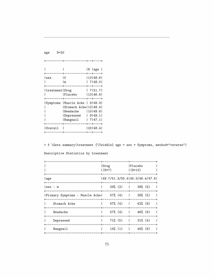
age N=20
+---------+------------+--+----+
| | |N |age |+---------+------------+--+----+|sex |f |13|48.6|| |m | 7|48.0|+---------+------------+--+----+|treatment|Drug | 7|51.7|| |Placebo |13|46.6|+---------+------------+--+----+|Symptoms |Muscle Ache | 9|48.9|| |Stomach Ache|12|48.4|| |Headache |10|49.6|| |Depressed | 9|49.1|| |Hangnail | 7|47.1|+---------+------------+--+----+|Overall | |20|48.4|+---------+------------+--+----+
> f \Gets summary(treatment {\Twiddle} age + sex + Symptoms, method="reverse")
Descriptive Statistics by treatment
+------------------------------+--------------+--------------+| |Drug |Placebo || |(N=7) |(N=13) |+------------------------------+--------------+--------------+|age |49.7/51.3/55.4|45.3/46.4/47.6|+------------------------------+--------------+--------------+|sex : m | 29% (2) | 38% (5) |+------------------------------+--------------+--------------+|Primary Symptoms : Muscle Ache| 57% (4) | 38% (5) |+------------------------------+--------------+--------------+| Stomach Ache | 57% (4) | 62% (8) |+------------------------------+--------------+--------------+| Headache | 57% (4) | 46% (6) |+------------------------------+--------------+--------------+| Depressed | 71% (5) | 31% (4) |+------------------------------+--------------+--------------+| Hangnail | 14% (1) | 46% (6) |+------------------------------+--------------+--------------+
75
\eex
\subsection{Conditionally Defined Variables}Another type of variable that is common in clinical reports is avariable that is of no interest unless another variable equalled acertain value. A common example is cause of death. We may want ourreport to contain the proportion of patients dying on each treatment,and for the deaths, we may want to know the proportions of deaths dueto each cause. For the latter calculation, the denominator is not thenumber of subjects in a treatment but rather the number of subjectswho died on that treatment. \code{summary.formula} will handle suchvariables correctly as long as they have missing values when they arenot pertinent. For example, suppose that the variable\code{death.cause} is \code{NA} if \code{death} is \code{F} (false)and \code{death.cause} is a categorical (or \code{mChoice}) variable if\code{death} is \code{T}. Then a \code{’reverse’} type summary will producethe needed proportions of \code{death} as well as \code{death.cause}.
\section{Alternate Approaches}\subsection{Literate Programming}In \emph{literate programming} as used in reproducible research (see\href{http://biostat.mc.vanderbilt.edu/StatReport}{\url{biostat.mc.vanderbilt.edu/StatReport}}),a single source document contains analysis code as well as text forthe report. This has been found to be easier to maintain and toresult in better documentation. Under \R, the \code{Sweave} packageprovides a concise syntax for mixing S and \LaTeX\ code for producingreports, as discussed in Section~16.3 of the course notes at\href{http://biostat.mc.vanderbilt.edu/StatCompCourse}{\url{biostat.mc.vanderbilt.edu/StatCompCourse}}.\code{Sweave} will run the S code chunks through \R, include Sprinted output in the report, and will generate \LaTeX\ commands toautomatically include graphics generated by the S code. Oneespecially nice feature of \code{Sweave} is the ease with which userscan insert variables computed by S into \LaTeX\ text without the needof the \verb|\def\varname{value}| approach described earlier.
\code{Sweave} is particularly well suited for non-recurringstatistical reports. Reports that are run after periodic dataupdates, for which the time spent polishing the report is well spent,are sometimes better suited to the customized programming methodsdescribed earlier in this document.
%\subsection{\LaTeX\ Server}%The UVa Biostatistics \LaTeX\ server allows the user to upload S
76
%output that contains a mixture of S commands and printed output and to%upload a \code{.zip} file containing all the postscript graphics files%for the report, and will run \LaTeX\ on the server, automatically%including graphics and making it easy for the user to provide legends%for the plots. The user can then download a \code{.pdf} document%containing the typeset report. See Chapters~2, 6, and 11 of the%course notes at%\href{http://biostat.mc.vanderbilt.edu/StatCompCourse}%{\url{biostat.mc.vanderbilt.edu/StatCompCourse}}%for more information.
\section{Data Preparation}For making nice--looking tables, as well as for havingself--documenting variables, it is important to spend time defininggood variable and value labels. If you are managing the data in SAS,for example, specify nice variable labels in a DATA step or using PROCDATASETS, and specify pretty value labels using PROC FORMAT. Bothvariable and value labels should use letter cases carefully. Don’tuse all upper case for either kinds of labels. Variable labels shouldoften contain units of measurements. An example of a good label is\code{’Serum Cholesterol, mg/dl’}. Better still, separate the\code{’units’} attribute from the \code{’label’} attribute of avariable:\bexlabel(chol) \Gets ’Serum Cholesterol’units(chol) \Gets ’mg/dl’# Alternate approach:mydata \Gets upData(mydata, labels=c(chol=’Serum Cholesterol’),
units =c(chol=’mg/dl’))\eexSome of the \code{latex} and \code{plot} methods in the \code{Hmisc} and\code{Design} libraries make special use of \code{units} attributes bytypesetting them in a different font or by right-justifying units incells of \LaTeX\ tables.
Binary variables are often coded 0/1. Good variable labels for theseare of the form \code{’Nocturnal angina present’}. Sometimes you maywant printouts to be more self--documenting. Then consider defining aSAS format of the form \code{0=’Angina absent’ 1=’Angina present’}.
You can always change labels and value labels after data are importedinto S. Here are some examples.\bexlabel(age) \Gets ’Age (y)’levels(pain) \Gets c(’None’,’Mild’,’Moderate’,’Severe’)
77
levels(pain) \Gets list(’Moderate/Severe’=c(’Moderate’,’Severe’))#Combines last two levels for subgroup analyses in which#there were two few patients with severe pain
levels(symptom)[3] \Gets ’Night sweats’ # fix one level
#Give fuller labels to levels of a binary variablenangina \Gets factor(nangina, 0:1, c(’Absent’,’Present’))
\eexThe Hmisc \code{upData} function provides a more general approach forchanging variable attributes. See Section~4.1.5 of\href{http://biostat.mc.vanderbilt.edu/twiki/pub/Main/RS/sintro.pdf}{Alzolaand Harrell}.
The Hmisc \code{sas.get} function is used to translate SAS data to anS data frame, carrying all data attributes. There are options tohandle special missing values. A typical procedure is to make anS program called \code{create.s} for each project directory.This program is run only whenever the SAS data changes. The createprogram should run the Hmisc \code{describe} function (and possiblythe \code{hist.data.frame} or \code{datadensity} function) to check eachvariable being analyzed for valid values and to make sure that keydata are seldom missing. Here is a typical \code{create.s}:\bexrct \Gets sas.get(’/my/data/path’, ’rct’, format.library=’/my/formats’,
var=Cs(age,sex,treatment,dtime,death,pressure),uncompress=T) #automatically uncompresses .ssd01 files
#Cs() quotes all names (doesn’t work if SAS names contain underscores)
describe(rct)\eex
If you run S interactively to develop and debug your reportingprograms, you will find it handy to make a pop--up window showingvariable names, labels, and value levels. To do this, issue thecommand \code{contents(rct)} after getting access to the \code{Hmisc}library, where \code{rct} is the name of your randomized trial dataframe. To pop--up a more detailed window with distributions for eachvariable, use for example \code{page(contents(rct), multi=T)} (in\splus). There is also an \code{html} method for the results of\code{contents}, to allow you to view metadata in a browser (withhyperlinks between variables and value labels). See\href{http://biostat.mc.vanderbilt.edu/twiki/pub/Main/DataSets/Cpbc.html}{\url{biostat.mc.vanderbilt.edu/twiki/pub/Main/DataSets/Cpbc.html}} forexample HTML output from \code{contents()}.
78

If you want to make variable label or value label changes in Spermanent, one option is to add the following type of statements afterthe \code{sas.get} command above.\bexattach(rct, pos=1, use.names=F)label(trt) \Gets ’Treatment’sex \Gets factor(sex, c(’f’,’m’), c(’Female’,’Male’))xx \Gets factor(xx, c(’a’,’b’), c(’A label’,’B label’), exclude=’Unknown’)# Treat ’Unknown’ as a missing value instead of a level...detach(1, ’rct’)
\eexA safer approach follows.\bexrct \Gets upData(rct,
labels=c(trt=’Treatment’),sex=factor(sex,c(’f’,’m’),c(’Female’,’Male’)),xx =factor(xx, c(’a’,’b’), c(’A label’,’B label’),
exclude=’Unknown’))\eex
See the Alzola and Harrell online text for much more information aboutmodifying and recoding variables and reshaping data.
The Hmisc function \code{Label} will generate S assignmentstatements containing all \code{label}s for variables in a specifieddata frame. You can edit the file output by \code{Label} to easilymodify labels you don’t like. Look at the help file for \code{label}for more information.
If you run \code{summary} output through \code{latex()}, caret signs invariable labels and sometimes in value labels will cause the word afterthe caret (up to the next space, comma, or end of string) to be superscripted.Also, the symbols \verb|< <= > >=| will be translated to the proper math--modesymbols such as $\geq$. There are other cases in which you may want toembed \LaTeX\ codes inside labels, e.g.:\bexlabel(x2) \Gets ’\$X\_{2}$’
\eexwhich results in \code{x2} being typeset as $X_{2}$.
\section{Inserting \LaTeX\ Output into non--\LaTeX\ Applications}You can use \LaTeX\ to create tables and other text or graphics and
79
convert the output file to encapsulated postscript (EPS) for insertioninto Word or Wordperfect ‘‘pictures’’. These pictures will not beviewable on the screen (a blank box with be displayed) but they willprint correctly as long as you remember to set your printer to apostscript printer before actually printing. Once you import thepicture you can re--size it (if you use a 300 dpi postscript driver,making the image larger will result in fuzzy printing).
Use the \code{dvips} program to make an EPS file from a \LaTeX\ dvifile, using the \code{E} option. Here is an example for the simplecase in which the document is only one page long (e.g., it consists ofa single table).\begin{verbatim}dvips -E -o doc.eps doc # creates doc.eps from doc.dvi
\end{verbatim}If you have a multiple--page \LaTeX\ document, you can tell\code{dvips} which page to store in a separate EPS file, for example,page 9:\begin{verbatim}dvips -E -p 9 -l 9 -o nine.eps doc
\end{verbatim}You can even have \code{dvips} put every page of the document into aseparate file. The files will be numbered e.g.\ \code{doc.001,doc.002, doc.003, \ldots}:\begin{verbatim}dvips -E -S 1 -i -o doc.0 doc
\end{verbatim}
In Linux an easy way to extract a particular page from a pdf documentis to use \code{xpdf} or \code{kpdf} and print that page to pdf. Thenit can be inserted as a picture.
Note that S plots can be output directly as encapsulated postscript orpdf, so you can include them in anydocument with no extra steps, as long as you stored only one plot in thefile. A nice way to pick out individual postscript plots and store them in aseparate \code{.ps} file is to use a postscript utility program called\code{psselect}, e.g. if you created 3 pages of plots in \code{myplots.ps} use\begin{verbatim}psselect -p1 myplots.ps myplots1.ps
\end{verbatim}to put the first page of \code{myplots.ps} into \code{myplots1.ps}.\code{psselect} can also be used to split out desired pages from apostscripted version of a \LaTeX\ document as an alternative to usingthe page number or section splitting options to \code{dvips}. Michael
80
Stevens of Duke University has written a program called \code{oneperpg}which will go through a multiple--page postscript file andautomatically create separate files each containing one page ofoutput, using \code{psselect}. For example, typing\begin{verbatim}oneperpg myplots
\end{verbatim}creates \code{myplots1.ps, myplots2.ps, myplots3.ps}.
Other ways to convert \LaTeX\ output to other formats are described at\href{http://biostat.mc.vanderbilt.edu/SweaveConvert}{\url{http://biostat.mc.vanderbilt.edu/SweaveConvert}}.As described there, \code{TeX4ht} can convert extremely complex\code{summary.formula} \LaTeX\ tables (including those containingmicro dot charts) to HTML. The resulting HTML file may be opened inOpenOffice and exported to an open document file, which can be openedand saved in Microsoft Word format. If the document contains pictures(e.g., micro dot charts), embed the pictures in the document afterexporting it to open document format, by clicking on the OpenOffice\code{Edit} and \code{Links} menus, highlighting all picture filenames using shift-left-click, and clicking \code{Break Link}. AnOpenOffice version of table \ref{s6a} may be viewed at\href{http://biostat.mc.vanderbilt.edu/twiki/pub/Main/StatReport/s6a.odt}{\url{http://biostat.mc.vanderbilt.edu/twiki/pub/Main/StatReport/s6a.odt}}.
You can insert the HTML file into Microsoft Word 97 documents, but ifyou save the document as a Word file rather than as HTML, specialformatting such as \LaTeX\ font size changes will be lost. This isbecause Microsoft is not consistent in how enhanced HTML commands areimplemented in Internet Explorer and in Word\footnote{I have nottested this under newer versions of Word.}. In addition to this
problem, \code{latex2html} does not convert all table commandsproperly; sometimes the program just stops in the middle of theconversion. If you have any math commands in the document,\code{latex2html} has to convert these to GIF images.\code{latex2html} is obsolete given \code{TeX4ht}.
In general, HeVeA (\href{http://pauillac.inria.fr/~maranget/hevea/}{\url{http://pauillac.inria.fr/~maranget/hevea/}}) does an excellent job inconverting simpler \LaTeX\ code to HTML, without the need for graphics imagesfor math commands. For some applications the resulting HTML caneasily be inserted into Word documents.
\section{S Documention}Use the command \code{?summary.formula} under S to getdetailed document of \code{summary.formula} and its \code{print},
81

\code{plot}, and \code{latex} methods.
\section{\LaTeX\ Code for This Document} \label{latex.code}{\small\verbatimtabinput{summary.tex}}
\end{document}
82