statistical treatment of strong...

Statistical Treatment of Electrolytes 529

limiting cases have been discussed: (a) the gas molecule is treated as an oscillator, ( b)as a plane rotator. In the first case the exchange of energy between the rotations of the gas molecule and the vibrations of the solid is negligible, whilst in the second the effect of the rotation is very small for hydrogen and larger for oxygen, taking the same repulsive field of the solid in the two cases. Under these conditions the energy exchange will be larger the larger the moment of inertia of the gas molecule.

Statistical Treatment of Strong Electrolytes

By S. L evine ,* Department of Physics, University of Cincinnati

{Communicated by J. C. McLennan, F.R.S.— Received March 6—RevisedJune 14, 1935)

1 — In t r o d u c t io n

By assuming the Coulomb forces between the ions of an electrolytic solution and by combining Poisson’s equation and Boltzmann’s principle, Debye and Hiickelf have developed a theory of strong electrolytes, satisfactory, however, only up to moderate concentrations. The approximate character of their method has been extensively investigated by a number of authors. Proceeding from the laws of statistics, Fowlerf showed that only for dilute solutions is Poisson’s equation valid in the Debye-Hiickel treatment, where phenomena on a molecular scale are involved, the omitted fluctuation terms becoming appreciable at stronger concentrations. Although Halpern§ claims that at no concentration of physical interest is such a neglect permissible, we may assume from more recent work|| that Fowler’s original conclusions hold.

Another objection is the use of the Coulomb law of force between two ions of charge ef and e„

F « = e <e,/D aA (1-1)

* Formerly at the McLennan Physical Laboratory, University o f Toronto.t ‘ Phys. Z.,’ vol. 24, p. 185 (1923).t “ Statistical Mechanics,” chaps. 8 and 13.§ ‘ J. Chem. Phys.,’ vol. 2, p. 85 (1934).II Kirkwood, ibid.,vol. 2, p. 767 (1934), and Fuoss, vol. 2, p. 818 (1934). See

also Onsager, ‘ Chem. Rev.,’ vol. 13, p. 73 (1933).

VOL. CLII.—A. 2 O

on June 16, 2018http://rspa.royalsocietypublishing.org/Downloaded from

http://rspa.royalsocietypublishing.org/

530 S. Levine

which is not justifiable for small values of In water, for example, the main part of D is contributed by the orientation of the water dipoles, and in the vicinity of an ion, a saturation effect will exist changing the value of D considerably. In addition, the polarization, van der Waals and exchange forces between the ions come into play at their close approach.*

To avoid the use of Poisson’s equation, Kramersf has applied the methods of statistical mechanics evaluating directly Gibbs’s phase-integral for the free energy F of the solution. Owing to the use of the approximate law (1.1), however, his expression for F is satisfactory only for very dilute solutions. In this article we shall be concerned with a more detailed analysis of Kramers’s method.

Various authors! have extended the original Debye-Huckel theory to stronger concentrations. Hiickel§ modified (1.1) by writing the dielectric constant as

D = D 0 - S SfTt, (1.2)i

where yf is the concentration of ions of the ith kind and the 8/s are empirical constants, so chosen that the activity coefficient is given correctly up to a concentration of a few moles per litre. However, there exist several objections || to Huckel’s treatment, and his results are useful only as interpolation formulae. Scatchard|| has shown in a qualitative manner that the form of (1.2) is doubtful, except for very dilute solution. He also indicated the importance of the non-ionic forces (i.e., polarization and van der Waals forces) between the ions and water molecules.

Sackf worked out the change in “ macroscopic” dielectric constant due to the saturation effect for very small concentrations, obtaining an expression similar to (1.2) but with much larger values for Owing to the doubtful assumptions and the neglect of several factors, his results are to be questioned. Indeed the law** D = D 0 + seems to be the correct one for dilute solutions. However, as the “ macroscopic ” dielectric constants may be quite different from the “ microscopic ”

* Any chemical hydration would also play an important part.t ‘ Proc. Akad. Sci. Amst.,’ vol. 30, p. 145 (1927).+ See Falkenhagen, “ Elektrolyte,” chap. 11.§ 4 Phys. Z.,’ vol. 26, p. 93 (1925).II See Orthmann, “ Ergebn. exakt. Naturwiss.,” vol. 6, p. 155 (1927), and Scatchard.

‘ Phys. Z.,’ vol. 33, p. 22 (1933).H 4 Phys. Z.,’ vol. 28, p. 199 (1927). See also Debye, “ Polar Molecules,” chap. 6,

and Orthmann, loc. cit.** Debye and Falkenhagen, 4 Phys. Z.,’ vol. 29, p. 121, 401 (1928); Wien, 4 Ann.

Physik,’ vol. 11, p. 429 (1931).




quantity involved in (1.2), this is not necessarily at variance with the form (1.2) used by Hiickel.

More recently, Bonino* took account of the fluctuation terms in Poisson’s equation by replacing the dielectric constant D 0 by the function

Here the X/s are constants and = /ca„ where a{ is the radius of the ion of the ith kind and k-1 is the “ characteristic length,” in the Debye- Hiickel theory. With given values of and by suitable choice of Xf, good agreement with experiment was obtained up to strong concentrations. The treatment, however, is of an empirical nature, E having no direct physical significance and acting only as a correction introduced to simplify the otherwise prohibitively difficult mathematics. There is no obvious method of calculating E from the microscopic properties of the ions and water molecules.

Finally we may mention the assumption of incomplete dissociation made by Nernstf to account for the heats of dilution of electrolytic solutions and the various experiments which seem to justify it and which find the degree of dissociation. In this paper, however, we shall not consider the question of incomplete dissociation of strong electrolytes but shall return to it on a later occasion.

The success of the empirical methods of Hiickel and Bonino suggests that the true form of the modified “ dielectric constant ” derived theoretically should enable a satisfactory extension of the theory of electrolytes to stronger concentrations. We assume a force of a more general type than (1.1), viz.,!

* Bonino, Centola, and Rolla, ‘ Mem. R. Accad. Ital.,’ vol. 4, pp. 415, 445, 465 (1933); ‘ R.C. Accad. Lincei,’ vol. 18, p. 145 (1933); Briill, ‘ Gazz. chim. ital.,’ vol. 64, pp. 261, 270 (1934).

t ‘ Z. Elektrochem.,’ vol. 33, p. 428 (1927). See also Falkenhagen, op. cit.+ The term may be regarded as representing' the “ specific interaction ”

of the two ions. The treatment given here bears some resemblance to that developed by Guggenheim who combines Bronsted’s theory of specific interaction with that of Debye and Hiickel; ‘ Phil. Mag.,’ vol. 19, p. 588 (1935).

(1.3)

2—Plan of the Paper

— s^lDrjj~ (2. 1)

2 o 2



532 S. Levine

where the team 0EtV/0rw acts as a correction, to be evaluated by a direct examination of the close approach of the two ions. Making use of the Gibbs’s phase-integral, it is found possible to replace (2.1) by an “ effective ” force

FW= eisj/(D &) ri f (2.2)

where 8,* derived from Efi, depends on the temperature and concentration. It is then shown that F has the functional forms

F = kTG [T (D - 8) Y '\ = N/cT </. [N*/T (D - 8) V*], (2.3)

where k is Boltzmann’s constant, N is the total number of ions in the solution, and V is the volume. We assume that the electrolyte is completely dissociated. The derivations of the relations (2.2) and (2.3) are given in §3.

In § 4 and § 5 a more detailed analysis is given of Kramers’s statistical treatment. It is shown that the various assumptions made by him are very plausible, although rigorous proofs are still partly lacking. In § 6 we introduce the modifications in Kramers’s treatment when the force law (2.2) is used in place of (1.1). It is shown that Kramers’s method can be extended to stronger concentrations provided the correction term 8 is known.

In § 7, the method of finding 8 is illustrated by choosing a particular expression for Ew. It is seen that the deviation of Kramers’s results from experiment may be attributed to the ionic association at greater concentrations. The actual form of E0 as obtained by examination of the saturation effects and the forces proper between the ions is not treated here but will be considered in a further communication. We conclude with a discussion of the method developed in this paper.

In the Appendix an examination is made of the generalized canonical ensemble used by Kramers. We see that, as a result of the introduction of such an ensemble, there will exist a correction term to his expression for F.

3—Development of the Functional Form

F = NkT(f>[N*/T (D - 8) Vi].

We shall consider a solution containing ions of the ith kind, each ofS

charge si9 i = 1, 2, s, so that N = 2 N,. Then the phase-integrali — 1

See footnote f, P- 535, for the interpretation of 8.



gives for the free energye - T lk T y N _ | j e - E / iT (J y i d Z i d z ^ , (3.1)

where, using (2.1),E = iS ' (£<e,/DrtV + E,v).* (3.2)

i, j = 1

Here jy, zl5 ..., zN, are the co-ordinates of the ions and E denotes the the instantaneous energy associated with the forces between the ions.

Differentiating (3.1) partially with respect to T, we obtainf


T 3F ~ T F ST = E — F ST’

where

E =

and

Ee<F- E>'*T dXl dyx dzx ... d z ^ j w = J S ' ^ + yi j = 1 E>rtj

Y = i S ' Eati,j = 1

|E = i h h ( - ±0T D 2 J T / ’" 3T "

01E 0Here •==,, y and ^ are defined similarly to E.01 01

Substituting (3.4) and (3.5) into (3.3), we obtain§

Now3F0e<

p T 3F _ 5 / i , T JD \ T 0 m xf _ t s t - e ( 1 + d 3 t ) “ d o t (Dy)'

j ... [ | 5 dx, dyt dzL... d z ^ / v *

_ 0E _ T , 9y “ 0^ . - +< + 0^ ’

(3.3)

(3.4)

(3.5)

(3.6)

(3.7)

* We use the symbol S' when in the summation over /, j , ..., m, i j ... * m.

t The treatment is similar to that given by Halpern, loc. cit.J We need not assume that y consists of a sum of terms E*y, implying linear super

position of the fields, but simply treat y as a whole.§ If we put y EE 0 in (3.6) and use the Gibbs-Helmholtz formula for the total internal

energy AU = F — T (dF/dT)v, we then obtain Bjerrum’s formula for heat of dilution



534 S. Levine

as is obtained from (3.2), writing

Then4, = S e,/Drt,.

i = i

- N _ N 0F N 0E = i 2 ef<h + y = * 2 - * S + y. (3.8)

t = 1 i = 1 o e i i = 1 o e i

Substituting (3.8) into (3.6), we obtain a differential equation for F,

T d D \ , 2^ 0FD d T / ' 0T

where

£, 3F / , , T dD \ . 3F OT-, . m2 E< + ^ T r r ) + 2T = 2F + y-(T> V> O , (3-9)

i = 1

x C r . v , 0 - 5 ^ ( D r ) + ( i + K ^ f sD d T i = 1 dzi (3.10)

The subsidiary equations of (3.9) form the simultaneous set

e«(T) = s* (T) ( l + J ^ ) / 2 T , i = 1, . . . , N, i.e., *t (T) = V*,TD,

F (T) = [2F (T) + z (T, V, e, (T))]/2T

= [2F (T) + x (T, V, Vi^TD)]/2T, (3.11)

F (T )T

^ x e r , v ^ T D ) <fr . KN + lj

where the k/ s are constants of integration. Hence the general solution of (3.9) gives

F = &TG (e£2/A:TDVi) + H (T, V, e£), (3.12)where

H (T, V, ef) - | fT * (T’ V^ /CfTD) dT, (3.13)

and we substitute k{ = e^/TD after integration. Here G signifies an arbitrary function of the N arguments ef2/^TDVi, IcV* being introduced to make the arguments dimensionless.

If we now assume (1.1) to hold, then y = 0 and we obtain

F = ATG (e,-2/^TDVi). (3.14)

It follows that if (2.2) is used, giving

E = i & M ,/(D - 8) r,,, (3.15)




the dimensional equation for F reads*

F = kTG(e 2/kT (D - S) V*), (3.16)

since we need only replace &TD by kT (D — S) in the integrand in (3.1). It is to be noted that (3.14) and (3.16) have the same functional form of their respective arguments.

Equating of (3.12) and (3.16) yields the relations from which § is to be deduced,

G (5a) = G tf) + H (T, V, sJ/kT , (3.16)

where we consider G (£a) as a function of = T (D — 8) V* on the left and G (£) one of £ = TDVs on the right. The introduction of Sf in (3.15) implies that we are replacing the quasi-canonical distribution in (3.1) by a different distribution, such that the same value for the free energy is obtained. This new type of distribution will have the characteristic steep maximum at the same value of E = E as in (3.1), and hence is legitimate provided the number of ions N is large enough.

It will be shown in § 6 that the Debye-Hiickel expression for the free energy F 0 is valid at limiting concentrations (V oo ), giving

F 0 = — S i.eGo = - $AN»5-» . (3.17)

Here s* = zfe, e being the electronic charge and z{ the valency of the

ions of the tth kind, k2 = ^ ^ iZ*2 an< A = tv introducings

a2 = e2 2 NjZ^/N, a constant if the composition of the solution doesi = 1

not vary. Then (3.16) yields as a first approximation to &

or- f AN»$r» = - |A N ^ - i + H (T, V, O ,

5 = H (T, V, e<)/AN**-* = H (T, V, e<) /TDVi\* A V N /* (3.18)

* Cf. Halpern, loc. cit.t N o mechanism is introduced for the interpretation of 8. It may be regarded as

defined by the relationJ_ (1 - e-khii)kT i,j=i (D — 8) n j _ dx, dy, dz, dz* = e - r /« VN = (M?, T) , say

where khij is introduced in (3.21). Assuming the existence of a solution of this

integral equation for D — 8 ,we have that D — 8 is o f the form D - J = / , ( ^ , T ) .



536 S. Levine

putting (1 — 8/D)- * ~ 1 + f ^ • Better approximations to 8 at higher

concentrations will be indicated in § 6.

Evidently the evaluation of H (T, V, e{) reduces to that of y, ~ ,

and . Since the contribution dE,7/ dri} in (2.1) represents a short-

range force, we can find y by successive approximations, by treating ionic encounters of increasing orders, as is done in finding the virial for an imperfect gas. This gives y in the form A 1jV + A 2/V2 + ..., where Ax, A 2, ...,are functions of the temperature and concentration. Similar

forms should be obtained for ^ and . It is necessary to treatasidTencounters of order greater than two by some method such as that developed for E by Ursell* and applied by the author.f In § 7 we shall only evaluate the coefficient A x, and no investigation of the higher terms will be attempted in this paper.

Since the free energy must be proportional to the total number of ions, if surface phenomena are ignored, it follows that F is of the form N ^(N /V ).} Comparing this with (3.16), we derive the dimensional equations

F = &TG [T (D - 8) Vi] = m T cf, [N*/T (D - 8) V*]. (3.19)

When the expression (3.2) is used for E, the phase-integral in (3.1) may be assumed to be convergent, but it becomes divergent when (3.2) is replaced by (3.15). Adopting the device of Kramers, we choose the energy function

NE' = * S ' (3.20)

i,j = 1* ‘ Proc. Camb. Phil. Soc.,’ vol. 23, p. 685 (1927).t ‘ Proc. Roy. Soc.,’ A, vol. 146, p. 597 (1934). The equation on p. 612 should

read

A2:; 8trrtje2D£T c°sh^f (+1 + « S + SnrtjS sinh (cosh Lt? — i

„ k T \

puttingsinh (sC/kT)~ e^/kT and cosh (e /AT) ~ 1.

As a result o f the assumptions and approximations made in this paper the final numerical results should be regarded as qualitative only.

t This follows from the form 2 N,-K (N</V) given by Halpern, loc. tit., if we assumet=ithe composition o f the solution is constant.




wherega = (1 - e-kh»)/(D - 8) (3.21)

andU 2 rjl_ — (Xi Xf (Tf y f iz i R V i *

% 4R02 (x. + x f + ^ + y f + iz. + z r u •

We choose X so large that (3.20) and (3.16) are practically equal for all configurations of the ions. Under these circumstances 1 and hence z f kT (D — S) retain the dimensions of a length, as is essential in our proof.

4—Examination of the Secular Equation in Kramers’s Treatment

In evaluating the Gibbs’s phase-integral, Kramers employed a generalized ensemble in which, for a given configuration of the N ions, there correspond N N samples. These are so chosen that for given charges of the ions 1, 2, k — 1, k + 1, ..., N, there are Nt- samples in which theXth ion carries the charge s, = zts. In place of (3.1), we now have

where 2 denotes the summation over the NN samples corresponding to a given configuration of the ions. A discussion of this special type of ensemble is given in the Appendix.

Kramers considers the relation (3.20) as representing a quadratic function of the N variables sx, e2, ..., eN, and imagines it to be given the canonical form by a transformation to principal axes,

We shall denote by Ar (X, fj,w), the determinant of the rth order, the diagonal terms of which are all equal to X, the other terms being given by ( k, l — 1, 2, ..., r, k /). Then the quantities bm, which dependonly on the ionic configuration, are the roots of the secular equation

yN e-FlkT _ j ... j N -N 2 e-E'/*T dx! dy\ dzx ... (4.1)

(4.2)i, j — 1 m = 1

AN (6i> ~ gij) — 2 arb*-r = 0, (a0 = 1, ax = 0), (4.3)

Sirh9 •••> ^

Pj G — hf • • • 9 K** We shall denote order of magnitude by ~ or O (...)•

(4.4)



538 S. Levine

We first examine the distribution of values of the bm’s. From the recurrence relation a0s„-x + a±sn - 2 + ... + + (« — 1) an~x = 0 thevalues of

sk = S b j ,m = 1

the sum of the k\h powers of the roots = 1, . . 2, ...,) are easily obtained.Denoting the average value of the N quantities bmk (m 1, 2 , . . , N) for a given ionic configuration by bmk, we have

— Oj z.c.j bfl (4.5)

>$2 — 2a o — 2 f

Thus

gijgj»S oi,j = l

N 2g2, /.£>., b j ~ Ng2,

= - 2 ' A2 (0, - gij).i,j = 1

(4.6)

where g = gij is the average value of the N (N — l)/2 quantities for a given ionic configuration. We assume here that ~ gij2.

s3 = — 3a3 = — i S ' A3 (0, — gp(r) ~ N 3g3, p, <r =

N 2g3. (4.7)

s4 = 2a 22 — 4a 4N2 '

Li, j = 1A2 (0, - gij)

X- i S'

i, j, k, l =A4 (0, - gf,a)

■ N 4g4, P, (7 = / , . / , k, l, i.e., b j ~ N 3g4, (4.8)

with corresponding expressions for the higher powers. We assume in (4.7) that gijgjkgki ~ (gij)3, and similar relations in (4.8).

To illustrate the evidently unusual distribution of values of the sr we replace (4.3) by the hypothetical equation

\(b,-g ) = i a 'r b*-r = (b + gr { b - ( N - l ) g } = 0, (4.9)r = 0

wherea '0 = 1, <tx = 0, a'r = (N )Ar (0, - g) = fN ) ( - (0, 1). (4.10)

To prove the identity in (4.9), we use the recurrence relation

Ar (0, 1) + 2Ar_1 (0, 1) + Ar_2 (0, 1) = 0,

from which, remembering that

Ax (0, 1) = 0, A2 (0, 1) = 0 1 1 0 = - 1,




we obtainAr(0, 1) = ( - l ) - 1 (r - 1).

so thata'r = (— l)2r_1 (r — 1) gr.

Hence the identity in (4.9) is true. Here, then, one root of (4.9) has the value (N — 1) gand the other N — 1 roots are all equal to — g. Hence Sl = 0, sk N*gfc, (k — 2, 3, ...), similar to the actual values of sk.

It has only been possible to indicate that the true values of the bm’s probably have a similar distribution to those of (4.9) and further analysis is desirable. If we treat the ar's as thermodynamic quantities, so that for the majority of the ionic configurations | — | < | |, aT beingthe average of ar over all configurations, then we may replace ar by ar in (4.3). Now Ar (0, — 1) = — (r — 1) gives the excess of negative elements over the positive elements in the expansion of Ar (0, — gp,). Hence, if all these elements are of the same order of magnitude, then ~ar is very probably negative for all r (except a0 — 1), leading to one positive root and N — 1 negative roots in (4.3). This suggests that for the majority of the ionic configurations the s are almost negative. To reconcile a distribution of bjs, almost all of which are negative, with the values bm = 0, b f ~ N 4'-1 g*, k — 2, 3, ... , it appears necessary to assume the negative bjs ( ~ — g) are all small, and there is one very large positive bm ( ~ Ng).

The purpose of this investigation is to show that all the negative s satisfy the condition

i + l p o . (4.11)

A tentative distribution function f(bfor the s may be obtained by use of Pearson’s method,* assuming the moments bm = 0, bm2 = Nga, bm3 = N2g3 as given. Then/ ( b) is the solution of the differential equation

1 d f _ b - a f d b c0 + c f

wherea = Ci = — N2g3/2Ng2 = — Ng/2, c0 = — Ng2,

i.e.,f(b) = A [b + 2g]-1+*/N e~2bi*° = A + 2g),

(4.12)

(4.13)

where b ranges from — c(j/lc1 = — 2g to oo, and A is a constant deter-• • • f 00mined by the condition f ( b ) d b = \ . For a uni-univalent electro-

J -2y

* See e.g., Jordan, “ Statistique Mathematique,” p. 244.



540 S. Levine

lyte zx = — z2 = 1, N x = N 2 = y , and the condition (4.11) becomes

bm> O (— 2 • 105), whereas the lower limit of (1 /DrtV) ~ 10~2,(V ~ 1). Hence we shall assume for the present that the condition (4.11) is satisfied for all the bm’s. It is possible, however, that some of the b j s may violate (4.11), and a modification in the analysis in § 6 would be necessary.

5—A More Detailed Analysis of Kramers’s D istribution Function for

Returning to the transformation (4.2), we have that the ym’s are related to the zk s by

N

Tm ^ Y (^*0k = 1

the coefficients ymk obeying the orthogonality relations

2 Y2m* = L S ymk = 0 m'). (5.2)k = 1 k = 1

Assuming the quantities | ymk | < 1 (we shall show | ymfc | ~ 1 /v 'N shortly), we follow Kramers and write the summation in the integrand of (4.1) in the form of an N-tuple integral over the values of the ym’s.

N __The bounds of y m are M and — M, where M = em 2 | \ ~ em \ /N ,

k — 1t m being the maximum charge present, but we may replace these bounds by —oo and + o o .

The mean value of y m isy m = 2 ymkek = 0, (5.3)

k = 1since

= c 2 N A /N = 0. (5.4)i = 1

Using (5.2) and (5.4), the mean value of y m2 is

y j = S ym* V = e2 2 N fzt2/N = e? = <r2. (5.5)k = 1 i 1

Also,N __ N

ym ym’ = s Y mkY m W = <J2 2 ym*ym'* = 0, (5.6)k = 1 A; = 1

from which Kramers assumes that the ym’s are statistically independent.




However, the relation (5.6) is not sufficient to establish this property, further conditions being necessary.

Kramers now supposes that the chance that y m lies between y m and y m + dym is given by a Gauss error function, /.<?.,

h (ym) dym = — L = exp [— y f / l a 2] dym, (5.7)(TV 2 Tt

so that the integrand in (4.1) is given by

N~N £ e~'E',kT =Nn

* + oo l\/2iz

— exp (5.8)

We shall now show that the assumptions made by Kramers are very plausible. We examine first the values of the quantities ymjS.. There exist the N relations*

N• bmYmp = 2 1,2, . . . ,N), (5.9)

9 = 1

which for each bm give N homogeneous equations to solve for N unknowns yml, ym2, ..., ymN. Solving in the usual manner, we neglect the last equation of (5.9) ( p = N), and obtain

{ml • ~{ml....... YmN A m 1 • A ?, (5.10)

where, if Am is the matrix of the system of the remaining N — 1 equations, A mk is the determinant formed from A m, by omitting the kth column of Am and multiplying by the factor (— l)1+fc. Thus ymfc is proportional to

Amfc = ( - l)1+fc . (5.11)

•••> g'N-l.t-lj S'N-l.t+lj •••> bm, 1,NNow if we treat A mk as a thermodynamic quantity,

(I A mkA mk | | A mk |),

and neglect the fluctuations we may replace A mk by A mk, its average value taken over all configurations of the ions, and therefore ymk by y mk- Now if the ions k and / are of the same type |ymV| = and if they are of different type, we may assume that |ymt| ■—< |ym+ t It follows from (5.2) that |ymfc | ~ 1 /N 4 which will hold for all 1,2, ..., N.

* See Courant and Hilbert, “ Methoden der Mathematischen Physik,” 2nd Auflage, p. 20 (1931).

t For a symmetrical type, | rmk \ == | y ml \ for all k, l.



542 S. Levine

We assume the statistical independence of the s for the moment and pass on to consideration of (5.7). In order that (5.7) be the true distribution function it is necessary that

Jm2B = 2^rf °a“’ •y- 2n+1 = °* (5.:12)

We shall proceed to find expressions for ( = 1, 2, ...).Using (5.1), (5.2), and (5.4), and applying the multinomial theorem,

y j = ( 2 Ymfcsfc)4 ^ 2 Ymfc4 + (2 ) TT £*2 • £J2 S ' Tmfc2 Yml2-Now

2 ymfc4 - 1 /N, S ' Yml2 Ymi2 = 2 Ymfc2 Tmi2 “ 2 y«*4 = 1 - 0 ( 1 /N).fc=i fc,i=i fc,i=i fc=iHence

___ 41 1 __ __V 4 — — — E 2 £ 2 /m 22 2’ S* ‘ 1

Similarly

41 I __ _22 2! £*2 • ei2

—a 4! 1 4|V 4 — ^ ^ Cf41

4! J_ 22 2!

IN *— a*

6 \ __ _ NU \ ~ t o V ' 6\ 1y m = sfc6 2 Ymfc6 + ( 2 £fc4 • el2 S ' Ymfc4 Yml2 + U / j f • e * S ' Ymfc3YmiA; = 1 k, l — 1 w ' • k, l = 1

+ (JT )3 J 7 £7 - «? • i2 . ^ x Ym?2 Ymfc2Yml2Here

2 Ymfc6 ~ 1/N 2, S ' Ymfc4Yml2 - l / N , | S ' Ymfc3Yml3 I < 1 /N ,A; = 1 k, l = l k, l = 1

2 ' Ym?2Ymfc2Yml2 = S Ym?2Ymfc2Yml2 ~ S ' Ymfc4Yml2j,A?,« = 1 j , M = 1 ^ 1 M = 1

- ! Ymfc6 = 1 — 0 ( 1/N ) — O ( 1/N 2).

Henceit = i

1—6 6! 6 6 _ ---- G b23 3 !

6 ! CT6

1N '

23 3 !We can similarly prove that in general

(2/Q !2” n ! c

2n _

(2ft) ! ff2n2" n !

1N- (5.13)



On the other hand, for an electrolyte of the non-symmetrical type,


bm* I = I e*3 2 ym*3 1 < IV *1 /N* ~ 0»/N*,A; = 1

lr?l = 1*7 s p < I*? 1/N*A; = 1 W / Ar, t = 1

+ 5X |efc3| «,VN*~ *5/N*.

For a binary electrolyte of the symmetrical type, e*2nfl = 0 and hence = 0. Thus in general,

| | < O (<t2"+1/N 4) < or (5.14)

so that we may assume the second of the relations (5.13). It follows that the Gauss error distribution function may be used and thus the relation (5.8) is valid.*

* It is not necessary to know y m2n+1 in order to show that (5.8) is correct. If the moments ymn of h (ym) are given and y m is assumed to range from — oo to + oo, then h ( j m) is expressed in series in Hermitian polynomials as

h (ym)1

Co + GW°) + f f H 2 0 ’, /a ) + ...g V2nwith y m/a as argument. Here H n (x) is defined by

ex t-w = s U n (*) tn/n !, n — 0

with the orthogonality conditionsr+oo

H n (x) Hn' (x) dx = 0 for n * n \J —oo _

= for n = n'.Using these relations, we see that

f + ooH„ (ym/a) h

(II)

(HI)

In particular c0 = 1, = c2 = 0. Substituting the Hermitian polynomial forn = 2p,H ,„ fje) = _ 2 p ( 2 p - l ) , 2p (2p — 1) (2p — 2) (2p — 3)

1 ! 2 2! 22+ ... + (— [)p ! +

1 ’ p \ 2*'in (III) and employing (II) and the first relation in (5.12), it is easily seen that c2p = 0. Thus (5.8) becomes

1h (ym) 1 + 3* H 3 0W®) + ^ H5 (ym/a) + ••• = = e-Vm'IW+ 2 r t (IV)

Remembering that H2n+! (ym/a) is an odd function, the relation (5.8) follows from (IV).



544 S. Levine

There is left to show the statistical independence of the ym’s. The necessary and sufficient condition for and y m. to be independent is that ( y l = 7 ^ = 0)*

rv\a rv\o ’where _____ __ ___

= ymV / ( j « 2)>/2 0 v V /2,

\ y j y ~ « - y j • y ^ i / K y J r 2 o, (5.15)

for all positive integral values of p, q. Making use of (5.12), it is readily seen that the denominator of (5.15) is of the order of magnitude of av+g. When not both of p, q are given, we have from (5.14) that

\ y 7 . y ~ 9\ < o ( a ^ i W ) .

The same is true of the other term in the numerator of (5.15) For example, using (5.4),

N N N N

y mym2 = . 2 TmiT mvV,'2 + T Y Y m'Jeiefcel = 2 Ym«Yi , j = 1 i = 1i = 1 k ,1 = 1

N ___ N ___ N^ Y m i Ym'j ~h ^ S Y r a f c Y m 'A ; Y m ' J £ fc ~ " b ^ Y m i Y m ' f c Y r a ' J ^ i ^ A ; ^ / *i, j = 1 k,l = l i ,k , l~ l

I ymym'21N

i = 1Y mi Y m i11 lN < |e i3| / N i < 0 ( a 3/ m .

When p, q are both even we have

I y T y J 1 (®w /n ).

For example, by (5.4), the non-vanishing terms in y mym* are

y m y m ' ^ Tmi Y m ' j £i ^ ^ Ym k Y m ' k Y m l Y m ' l ^ k £ZM = 1 k, l = 1

N= 2 ' Ym*YmvVeia + 2 Y«<2Y«'*V + ( 2 Y m k Y m 'k ) 2i,j = l i = l * = 1

- 2 2 Ym'i2YmtV • £i2>i.e.,

* = i

I «<2 • e,2 | = | Tm2Tm 2 “ Tm" • JV* I = O K /N ).

* 5 ^ Borel, “ Traite du Calcul des Probabilities et de ses Applications,” vol. 1, part 4 (part 2), chap. 3.




We conclude that | r p)4| < O (1/N*) of all q, and hence the can be taken to be statistically independent.

6—Evaluation of the Free Energy of the ElectrolyticSolution

Using (4.13), the value of (5.8), as derived by Kramers, is

n -n s e - w i k i = n (i + a t ) * =m=l\ kT /

<72 'n a / kT XT* 1Ym ) ^ { ~ ~ ^ ’ ~ 8ki)\ (6,1)

where= AN_i (U v-g'u) = An-*, say,

a2/(D — S) kT = (3/(1 - 6 (N) ) and 8 kl (6.2)

Here (3 = a2/DAT and for convenience we indicate the argument N only in 6 (N) = 8/D, 8 being also a function of T and V. We regard D and therefore (3 as a function of T only. Substituting (6.1) into (4.1), we obtain

F = — kT log AT* = \kTlog X* = log A j (1, «*'„). (6.3)

Here the bar denotes the mean value taken over all configurations of the ions of the volume V and we neglect the fluctuations of AN, replacing A^-4 by An-*. _

We proceed to derive a general expression for AN. Differentiating An partially with respect to (3,

0An 0 l N 3a t .N A A0(3 “ 0(3 A An la ’ 8 'n)\_ a ^ An + aN0f An l a ’ 8 'kl) (6A)

Remembering that the mean values of the subdeterminants of the

diagonal terms of AN ( ^ , g'klJ are all equal, we have

1 a ( 1 9 a / l - e ( N ) , \ N 0 a 5 / 1 — 6(N)2 n l 1 8 k l ) ^ n \ n ‘ 9 8 kl I o ^ N —1 \ n 90(3 V 0(3 p a2 0(3 PRetaining the first two terms in the expansion of 6 (N — 1),

■ g kl ) -(6.5)

*N-11 - 6 (N - 1)

P g n 1 - e (N) 106(3 T (3 0N ’ * “

1 - 6(N) \ ( N - 1) 06 * /I — 6(N — 1)a 9 8 k l ) "T" Q 0N ^N-2 l o >

, n - e (N) , 1 06 t - 1 r i - e (n ) in-! + L----- 3----- + B0n J “ L----- 3----- J

00 (3 0N

_ (N - 1) ae_ |~1 - 6 (N) 1 06 ]N(3 0NL p 3 0NJ

g

. (6.6)

VOL. CLII.—A. 2 P



546 S. Levine

Since N gjq''"' 1 (6 ~ 1 and for dilute solutions 6 < 1), the last three terms on the right of (6.6) are of the order of magnitude of

[ 1 - 6 (N)]N_1/pN_1.

Using the hypothetical case (4.9),1 - 6(N)

P ’S kl

N — 1 2r—1' S ( - 1)

r = 0

N - l - r

(6.7)with an analogous expression for AN_2. Since (3 ~ 10~7, it follows that we need only retain the first two terms on the right of (6.6), the others being negligible in comparison. This gives us a recurrence relation yielding the series

/ I — 6 (N)V P

1 - 9 (N - 1) P

(N - i) ae tp 0N N~2 (6.8)

Retaining the first term on the right of (6.8) and substituting the thereby modified form (6.5) into (6.4) we derive

3An _ N 0a ^ A_ N 0a 3AN“a ir _ a 3 p 1 N N-1' — a ap I N ’

to a first approximation. The solution of (6.9) is of the form

H «N,V) = VI N ip1(1 - 6) V*/J

«N*\TVi /J ’

(6.9)

(6.10)

where a>N is a second functional form for AN obtained from (3.1) and (6.3). On differentiating (6.10) partially with respect to (3 and N and eliminating $ from the two resulting equations we arrive at

I K = log to, n = aNi/Vi, (6.11)giving _

An = wN = exp [ - 2K (pN)* V-* (1 - 0)"»]. (6.12)

Here K = f V™, as shown by Kramers. Hence

F $NkT log w = - fV™ (pN)* V-* (1 - 0)-*

= _ S ^ (1 _ 0)-t, (6.13)i = l J i->

which corresponds to the Debye-Huckel second approximation.




As noted by Kramers, it follows from (6.12) that for larger concentrations, the ratio between Ax and An_ i will deviate more and more from unity, so that the approximation in (6.9) is no longer permissible. Proceeding in the manner adopted by Kramers, we have

An Ax 1 = [co (xN)]N - [co (XN_!)]N 1

= [<*> ( ^ n ) ] N _ 1 [ “ ( * n ) — ( l —63 (■%) 3xk\H 11co(x)N 3N / J

- [ - w - exp( - !v ( l r & ) ] • <6-14)

where xN = a3N/V is considered to be a function of N and co' (xN) = dco(xN)/c/xN. Then (6.9) becomes, omitting the argument of co and co',

ap3NcoN_1 xN 3a co'

3 p aNcoN_1 3a

a 3pco — exp / Nco' 3xn\

\ co 3N /J’ (6.15)

i.e.,3xco' = co — exp xco' N 3x\

co x 3N /r xco'/, .

" “ expL“ — ( 1 +3N 30 \~|

1 - 0 3N /T

dropping the suffix on x. Here 3N 30 1 - 0 3N

(6.16)and hence co is no longer a

function of x alone, the discrepancy arising when co (xN_x) is expanded in (6.14). To overcome this difficulty we assume T is kept constant so that x is a measure of the concentration, and we write

+ (x) = 3N 30i - e 3N;

On putting 0 = 0, (6.16) reduces to

3x0co'0 = co0 — exp ( — 0 (6.17)

where co = co0, x = x0, co'0 = ^ 2 when 0 = 0. Substituting

x° — — t0, (6.17) becomes

co0 = e'° I (1 +.3r„), which on differentiating with respect to x0 leads to (t'0 = ^2.

\ U X q

(6.18)

0 o _ _(2 3;0) t 0x0co0 1 + 3 tQ

2 p 2



548 S. Levine

with solutionK2x0 = ~ * 0 = *o2/(l + 3t0)3 = ^ P3 ^ • (6.19)

Here (6.18) and (6.19) are the parametric solution obtained by Kramers.We now treat (6.16) in a similar fashion. Putting xco'/« = — /,

(6.16) becomesw = et(1+*7(l + 3t) = e*e*/(1 + 30, (6.20)

introducing x = f 4* Differentiating logarithmically gives

_ t = — = ty'tx + (1 + <|>) t'x - 3f'x/(l + 30,CO

ordx_ (2 — 30 — 41 (1 + 30 m

~x ~ (1 + 30 (1 + Vx) 'The solution is

wherev(t)

Kx2x = Kx2

ff 2 - 3 1 J U (l + 30

p3 N(1 - 6)3 V

1-l + i>'x - 1

t2ev(t)(1 + 303 ’

^ ) dt" * ( l + f x ) j '

(6.21)

(6.22)

We assume in (6.20) and (6.22) that x and hence ^ (t), x (0 and v (t) are known functions of t. Then the solution given by (6.20) and (6.21) replaces (6.18) and (6.19).

We now derive

l0g^' 01SL1 0F N 1 </<o

2 o) dx3N; + \ log «

and

1 ~ g =

= i [t + x

V 0F _ /,NkT 0V 2 V '

log (1 + 30 + * 4> ( 0 ( 6 . 2 3 )

3VD (1 - 6) 0V,

To obtain (6.23) and (6.24), we use the relations

~ ) 4) (0.

— = - to (0 = - tCOi _ l -\- 3t dy l / T+ | (1 3/) dv

2 - 3 td t / L 2 — 3/0X X / ! 3V 08'

D (10X0n :

XN D (1 - 6) 0N

_080) 0V/

3Nz,-2 - 2SN..Z,2

1 = 1

x T

(6.24)

(6.25)




as may be deduced from (6.20) and (6.21), noting that 0 = S/D. On putting 0 = 0, (6.25) and (6.26) reduce to Kramers’s expressions

log/, = h ( \ - ~ i (1 + 3/), 1 - g = L (6.26)M s n a ‘ I 2\ i=1 /

To indicate the modifications produced in the osmotic coefficients, we develop (6.20) and (6.21) further for dilute solutions. According to (3.18), a first approximation to S is

so that

S ~

3N 30 _ 3 S 1 — 0 8N 2 D (1 - 0)

[Xi (T) x* +

(6.27)

(6.28)

where ^i(T) = §Xx (T) (TD/(3)!. Since we shall not evaluate \ (T), ... in this paper, an estimate of S is obtained from the work of Debye and Hiickel. Writing their expression for the electrostatic energy as

P _ * N ^ 2 e2/c _ A W kT _ AN kT' t- 1 2D' 1 + ko[D (1 + Kaf TV ] [(D S) TV*]4 ’

where a is the “ average ” radius of the ions, we derive

1 - 0 = 1 - S/D = (1 + *<!)», (6.29)

giving to a first approximation

A = - f K f l = - A ( ttp N J a = _ 4 * * * . ( 6 . 3 0 )

Then(x) - 2 y'Tu (1 — 0)‘x4tf ~ — - x4 = jj x4, / = (6.31)

Writing 1/(1 + <]/*) = 1 — - [XjX4 and retaining the term x4 only, we

derive for (6.22)v(0 = - [Ai 4 + 3/> dt. (6.32)w 2 J t(l + 30 v

Substituting x4 = tjK (1 + 30* as a first approximation, (6.32) becomes

Vi (0 = [i.x (2 + 3Q3K (1 + 3 0 :

(6.33)



550 S. Levine

where Ax is a constant. Then (6.22) reads

Ki2*! = t2(1 + 3

exp jxi (2 + 3 L3K (1 + 30*

+ Ax . (6.34)

If we assume that (6.34) must reduce to (6.19) for small t (neglecting all orders higher than that of t2), then Ax = — 2[x1/3K, Kx = K.

Continuing this process {i.e., we now use (6.34) for x*), we obtain for the second approximation

K = exp Jfi (2 + 3 L6K (1 + 3

K2* 2 = (1/ 303 exP [2(^-1)].and for the third

J£i3KJ ’

(6.35)

(6.36)

*’*(')=!{(’°8 *•+f+o 5+rxT2+■")_ ( 1 + n 5 + r o * + •••)}■ (6-37)

with the corresponding expression for x 3. It was found that (6.35) and (6.37) gave practically the same results, so that there was no need for higher approximations.

Using (6.31) and (6.36), we can now find x (t) and from (6.35) v (t). Further, according to (6.29),

3v as _ kuD (1 - 6) 0V 1 + ’

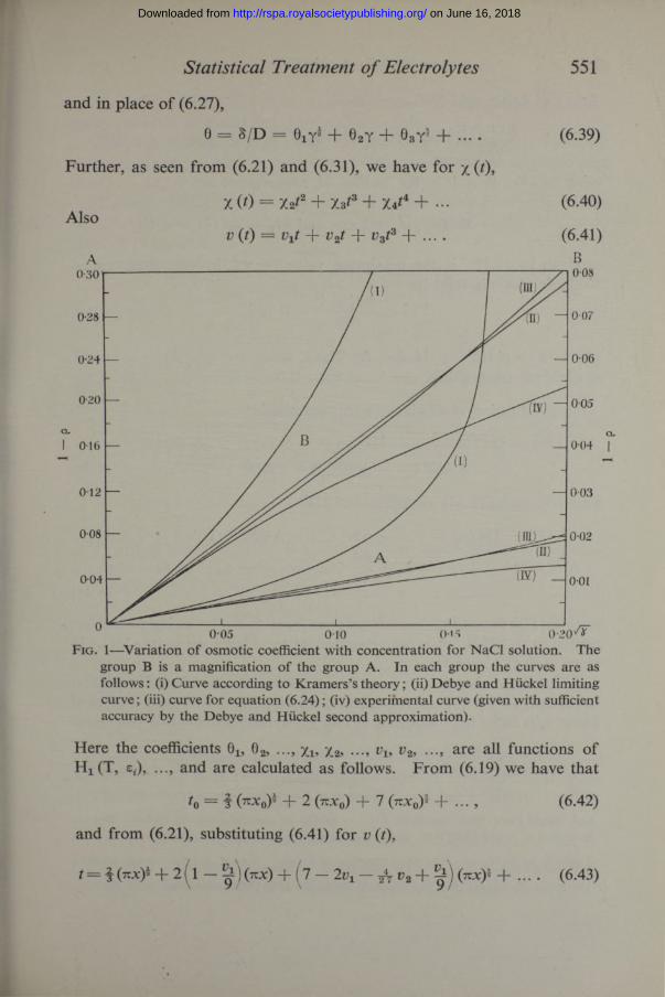
Thus the evaluation of 1 — gas given by (6.24) could be carried out for dilute solutions of NaCl, fig. 1. The values of x, and hence of the concentration y (mols per litre), were found from (6.21) and (6.29). At T = 291° K, D = 81, (3 = 7 - 0 4 .10"8, 4 - 0 2 . 10"8 cm, ^ = - 2-02.The deviations from experiment at higher concentrations are to be expected as the neglect of the terms in x, x% ..., in (6.32) is no longer permissible. According to (6.19), x0 and hence y reach a maximum at 2/3, y = 0-028, and then begin to decrease with further increase of t (and therefore of F). This anomalous behaviour no longer exists when we use (6.21), as is illustrated by the form (6.36) for dilute solutions.

We shall require the general form of v ( ) and / (/) and hence of S and H (T, Y, s*) at greater concentrations. As will be seen in § 7,

H (T, V, et.) = Hi (T, ef) N2/V + H 2 (T, zt) N3/V2 + .. . , (6.38)




and in place of (6.27),

0 = S/D = 0lTi + 02y + 03y5 + ... . (6.39)

Further, as seen from (6.21) and (6.31), we have for / (0>

X (0 = M 2 + i 3t3 + ••• (6.40)Also

v (0 = Vyt + v2t + v3f + ... . (6.41) A B

I 016 004 |

Fig. 1—Variation o f osmotic coefficient with concentration for NaCl solution. The group B is a magnification o f the group A. In each group the curves are as follows: (i) Curve according to Kramers’s theory; (ii) Debye and Hiickel limiting curve; (iii) curve for equation (6.24); (iv) experimental curve (given with sufficient accuracy by the Debye and Hiickel second approximation).

Here the coefficients 0l5 02, ..., Xi> X2> •••> vu v2> •••» are all functions of Hi (T, e,), ..., and are calculated as follows. From (6.19) we have that

t0 = iO o)1 + 2 (7tx0) + 7 (xx0)J + ... , (6.42)

and from (6.21), substituting (6.41) for v (t),

t = | (nx)i + 2 (l - | j (nx) + (7 - 2v1- ^ v2 + S') (nx)i + ... . (6.43)



552 S. Levine

Here * (6.42) is valid for

| t 0| < R2 f f l -2 = 0-133, or for NaCl, jc0 < 0-0076, y < 0-018, OiVLo

using (6.19); R = | is the radius of convergence of

Xq* S drt0r, dx = | and M 0 = ( |) = 0 • 10,r = 1

as given by (6.19), is the maximum value of x 0* in the given range. Similarly (6.43) is valid for

1 ' 1 < = ° '° 98’

where M = x* ( |) = 0-14, i.e., for NaCl, when x < 0-0041, y < 0-013, as obtained from (6.36).

On substituting (6.42) into (6.18), we obtainf

G (5) = |N log O)0 = - |N (7tx0)i - N (7TX0) - |N (n x t f - ...= - | A W 5~» - A2N 25~3 - l A3N= 5-1 - ... . (6.44)

Similarly, using (6.20), (6.40), and (6.41),

G , (50 = |N log o) = — | A W 5 r » - A2N 25~3 (1 - - I ®i)

- A3N ^ - t ($ — i v 1 - | X2 + ^ + A - A Xs - A »«) - - •(6.45)

Here G x (5X) is not the same functional form as G (5), owing to the fact that o) in (6.16) is not a pure function of x. Hence we write G x (5i) in place of G (50 in (6.45).

A first approximation to § has actually been obtained by using the first terms only in the expansions of G (5) and G x (5X). This gave (A and hence v (t) and / (t). Knowing vx and -/2, we may use the first two terms

* See Dienes, “ The Taylor Series,” p. 260.t According to Halpern, loc. cit., the free energy F, given by (6.44), may be written

as F = — J (k /3D + C/<2 + ...) a function o f J = 2 N,Sj2 only (since k2= 4 ttJ/D^TV),<=iand hence must have the form F = — J/c/3D in contradiction to (6.44). But we note that C = J/4 (DAT)2 N , which Halpern considers to be a constant, involves both

J and N = E N*, i.e., F is not a function o f J only. Indeed, if J/N = constant, then i - 1

the form F = J/(J) used by Halpern reads F = N<{> (N) as assumed in (3.19).




on the right of (6.44) and (6.45) and substitute in (3.16) to obtain a better approximation to 8 and hence to v (t) and / (t).

This process may be continued until no longer necessary. At higher concentrations we need to find the analytic continuations of (6.44) and (6.45).

At greater concentrations, equation (6.17) itself becomes unsatisfactory, for it is necessary to include the second term in the series (6.8), so that, in place of (6.9), we have

Noting that

9An = N 0a 9(3 a 0(3

As _2 —

"a a I N 06 X 1A N - 1 T j __ Q AN_2 I . (6.46)

< o W P - e x p [ - 2 N “ * J ] , (6.47)

obtained by the same method used in (6.14), (6.46) gives, in place of (6.16),

3xto' = to exp — ( l + +)toI ^+ | exp 2xto' ( l + < 0 -(6-48)

Substitution of — t = xto'/oo leads to

- - r T 3 ? (1 + f c4 (6-49)

The corresponding form for x is derived in the same manner as in (6.21), giving

dxx

with solution

(2 - 3p - <H1 + 3Qt (1 + 3t) (1 + dt + (f> (0 dt, (6.50)

K2* = JYT y f eX(t)’V (0 = O (0 + f <f> (0 dt. (6.51)

Here v (t)is given by (6.22) and

A (A = 1 g*^ W ±O' + x 'H ] dx *W 7 t(1 + <{/x) (1 + +g‘e*/3) dt '

Successive approximations to V (t) and hence to x and to may be obtained as before. We shall not proceed further with the solution at this stage of the theory.

7—Evaluation of y for the Form Ei7 = x j(n — 1) r , / -1

We shall illustrate the method of finding y by choosing a special form for E„ in (2.1). A first approximation to y, valid for dilute solutions,



554 S. Levine

may be obtained by treating only binary encounters of the ions. Suppose the solution contains two types of ions s3- and sf, in number and N, respectively, such that N f = /N, Ny = y'N, = 1. We assume aforce

Ffi = S!Sj/ (7.1)so that

Ew = X „ / ( » - l ) r „ - 1. (7.2)

The suffixes m, n, p shall refer to the pairs (i, i)» 0", y), O’, respectively. The contribution to y = 3 2 ' E<# from binary encounters is given by

the sum of three terms corresponding to encounters of the pairs, viz.,*

i An y - n + 3Jo n — i ’ M

^ (e«e,/Dr«, + X„/(n - 1) V 1)] dri}

- _ 2 4tcN^N,- f00 X„m , n , p V

X exp

4ttN 2V m,n,pYl

r—n + 3V (An y ( 1)T | 1 s<eiV f°° ™ r-, « , * » - l r - 0 T ! WT D / Jo

x e x p [ ~4ttN2 2 J S l

m, n,p (n - l)2 L(« - 1) kT.-(»-4)/(«-l)

x si .e.,

( V r i- t/(»-d -i- _ 4^

VArDTV L(n - 1) AT- 1 V n - 1 /(7.3)

y = ^ n 2 n j B„r r '» - v ,Y ^ ^ "nrV m, n, p t = 0

whereA , = 0 ^ [X i,/A:(/i - 1)]‘»+®/‘- « v'„ = 5— i , v„ = ---- ?,n — 1 n — l

B - ( - ”T t ! \AD/

— T/(»—1) / x + h — 4\A: (ft — 1) 1 )

• N 0Y 0Y .Similar forms may be obtained for 2 e* — and -^L provided E„ is ai = l c l

function of and T. Substituting the resulting expressions for

y, 2 e< p - and | l into y (T, V, s,),i = 1 oei c l

X

* See Jones, ‘ Proc. Roy. Soc.,’ A, vol. 106, p. 463 (1924).




as given by (3.10), it follows from (3.13) that H (T, V, e3) is of the form H x (T, e j N 2/V. A treatment of ternary encounters yields a term H 2 (T, £j) N 3/V2, and in this way we obtain the series (6.38).

A negative value for y implies a tendency for the ions of opposite charge to associate. The (negative) contribution to y from (i, ) encounters would be greater than those from the and (J, j) interactions,*

being an attractive force. If stronger association exists with solvents of low dielectric constant, y and hence § would become appreciable even for very dilute solutions. This would explain the failure of the Debye-Hiickel theory with electrolytes of such solvents and confirm the applicability of the concept of ionic association as was carried out by Fuoss and Kraus.f

If we assume the ions to be rigid spheres, we let °o subject to the conditions au = lim An,/(n-1), where <rfJ- = ai + being the radii

n —> ooof the ions i,j, with a similar treatment for m and p. However, in this case lim y = 0. This does not in any way invalidate the method developed here, for there certainly exists a term E,v ^ 0 due to saturation and hydration effects and to those forces other than the Coulomb between the ions themselves. We shall endeavour to evaluate Eti in a further work.

Finally, there is need of a more satisfactory estimation of the roots b m in §4, since the existence of such roots violating the condition (4.15) produces a change in the form (6.3) for the free energy. A more satisfactory proof of the validity of the Gauss distribution law in § 5 is also desirable. The problem of incomplete dissociation may be investigated if EjV, yielding the work of ionization, is known and if the internal partition function of the solute molecules can be calculated. For the equation of mass action would at once lead to the degree of dissociation. We shall return to these points on a later occasion.

A ppe n d ix

We proceed to examine the legitimacy of Kramers’s ensemble. In the usual form of generalized ensemble, the integrand in (3.1) is replaced by the summation J

S exp [— E (vt.)/£T — 2 a* vj, E (vt) E (vl5 ... , v4), (A .l)vi* ... s=0 i = l

* According to Bronsted (see also Guggenheim, loc. cit.) the contributions from 0, 0 and (y, j ) pairs would be negligible; ‘ J. Amer. Chem. Soc.,’ vol. 44, p. 877 (1922).

t ‘ J. Amer. Chem. Soc.,’ vol. 55, pp. 476, 1019, 2397 (1933) and later papers.+ Cf. Pauli, ‘ Z. Physik,’ vol. 41, p. 81 (1927).



556 S. Levine

subject to the conditions

^ J r ( + “‘ = 0 < ' = * • * .......*>• <A-2>

There exists an extraordinarily steep maximum in the number of samples in the summation (A.l) at vf = N f (i = 1, 2, 5), such that only for a variation of v2 from N a given by

AN,/Nf = | v, - N f | /N, < 0 ( 1 /N » ) , (A.3)

is the number of samples in (A.l) appreciable. Further, if Fn is the free energy obtained when (A.l) is used in (3.1) and Fx is that given by (3.1) itself, then the difference between these quantities is given by

I (Fir — F^/F j | ~ (log N)/N. (A.4)

We need to prove that similar properties hold for the distribution of samples employed by Kramers in order that the relation (4.1) be valid. This distribution is governed by the multinomial expansion

(Na + ... + NS)N = 2 N ! fl (N/Vv*!)vit... v =0 i *= 1

S N ! exp T S vf log N f”l / II (vf !), (A.5)vx, ... i's = 0 *— i = 1 -J/ i — 1

where 2 = N, and the term N ! II (NfH/vi !) represents the numberi = 1 = 1

of samples which have vi ions of kind 1, 2, ..., s). Under theseconditions (4.1) becomes

y N e - ¥ n /tT

X exp

N

N2

vx, ... vs

I 2 v* logL i = 1

N !

=° II (vt. !)i = 1

^ - E (vt)/A:T | dxx dyx dzx ... dzN, (A.6)

so that here oq = log N JN .We shall only illustrate with a binary electrolyte, containing N x + N 2

ions. Here (A.5) becomes(Nx + N 2)n = 2 (N ) N 1N- ' N / . (A.7)

V =0 \ v /

Putting A = v — N 2, the average value of (A/N)2 is

A^N2 N N

l (v - N 2)2/N\ _ 0 N2 V v NxN-*' ' i . (A.8)




Further, by applying Stirling’s formula, the ratio of a typical term in (A.7), N ! N 1Ni_A N 2 3+a/(N1 — A) ! (N 2 + A) !, to the greatest term, N ! N 2n>/Nj ! N 2 !, is

(1 + A/N2) - n* (1

1 -

A /N i) -* ' (1

N

A / N ^ l l + A/N2)-

2N1N 2A3

A2+ 0 k r 2 + - ~ exP -N A 1 2

2N1N 2(A.9)

if A ^ N s. It is seen from (A.8) and (A.9) that for A2 > N the number of samples decreases very rapidly and thus (A.3) is true. Consideration of more complex electrolytes gives similar results.

For a binary electrolyte (A.6) gives

e -F n/*T _ (A.10)

Retaining the first three terms in the expansion ( A = v — N 2)

F i(N x - A ,N 2 + A) F1(NB N J + ( , - N j ( 1| r - ^ F I

- n 2)2/ a2 V0N 2

0 \2- w ) F' + , (A.11)

we geto —AN o(Fh-Fi)/*T _ eN N ..

Xv n2)2_ o (A. 12)

where

II 1 0?n 2 -3 N 1) Fi = 1° 8/ . / /» ~ > .

_ 1 ( _ L )2 F ~ 12kT vaN2 01V bl N*

Neglecting the term in (jl, we have

e~,-ANo N

^-AN2 ^

2 eKv( N ) N1N- ,/ N /V = o ^ V /

[Nj. + N 2ca]n = exp [ N log {1 + ^ (e* - 1)} - XNa

- A N j

exp

« + § ( « * - » T

1 _N22 V N + N,X3 ?N2 2N22

N ^ N2 • ) + . . . ] , (A. 13)



558 Statistical Treatment of Electrolytes

assuming | (N2/N) ( eK — 1) | < 1, giving

| (Fn - Fl)/Fi | — 5n ( i + § ) X 2 + - ‘ (a -14)

If, for the symmetrical type (Nx = N a = N/2), we assume l o g / = log/* then X = 0, and this is equivalent to the condition (A.2), so that (A.4) holds. For the non-symmetrical type, however, X ^ 0. Forexample, if for z%= — 2zL, N x = 2N/3, N 2 = N/3, we use the Debye-

2|.Huckel limiting expression for the activity coefficient lo g / — — — i ,

ZL-/q/C Xwe find at T = 291° K, X = 0-59. Then at y = 0-01 (A. 13) becomes | (Fn — F1)/F1 1 ~ 0T6,* using the form (3.17) for Fx. Since the greatest contribution to the sum in (A. 13) comes from v ~ N , then the neglected terms in the expansion (A. 11) must be considered. Indeed, if Fr is given by (3.17), it is seen that g. is a negative quantity, so that (A. 12) will give a smaller value for | (Fn — Fx)/Fj: | than (A. 13).

With symmetrical electrolytes, X departs from zero as the concentration increases, so that a correction to Fn will be necessary. A first approximation to this correction may be obtained by substituting

x = _ F r (aN 2 Firinto (A.13). For the high-valency types where it is more probable that l o g / ^ log/* for dilute solutions and also in the non-symmetrical cases, there will be an appreciable difference between Fr and Fn . This is in accordance with the failure of the Debye-Huckel limiting law for such types of electrolytes. The applicability of Kramers’s generalized ensemble in these cases thus becomes questionable.

In conclusion, the author wishes to express his sincere thanks for help received from Professor E. F. Burton, Dr. C. Barnes, and Dr. J. K. L. MacDonald of the Department of Physics at the University of Toronto, and from Professor I. A. Barnett of the Department of Mathematics at the University of Cincinnati.

The writer is indebted to the University of Cincinnati for a research fellowship enabling him to continue the work on this paper.

Summary

In this paper, a theory of strong electrolytes is developed by an application of statistical mechanics. The method of Kramers is adopted and

* If we use the second approximation of Debye and Huckel, then for K 2S 0 4, a = 2 -6 9 . 10-8, we obtain | (F„ - FO/Fj | = 0 - 1 3 .



Creation of Electron Pairs 559

it is shown that if the ordinary Coulomb forces between the ions is used, under certain assumptions, his treatment is valid. Owing to his use of a special generalized ensemble, a correction is necessary which is small for low-valency symmetrical electrolytes but which may be quite considerable for the non-symmetrical cases. The deviations from the inverse square law, due to the saturation and hydration effects on the water dipoles and to the polarization, van der Waals and exchange forces between two typical ions iand j is accounted for by means of a correction term Eif in the expression for their energy of interaction. It is shown that the addition of this term is equivalent to a modification of the dielectric constant D to D — 8, where 8 depends on and is a function of the concentration and temperature. The extension in Kramers’s theory as a result of this new type of force is given, and it is seen that with the proper form for 8 the method proposed here should satisfactorily describe the properties of electrolytic solutions at strong concentrations. Definite numerical results cannot be obtained until 8 is known. The attempt has been made to avoid the essential difficulties in the original Debye-Huckel theory.

The Creation of Electron Pairs by Fast Charged Particles

By H. J. B h abh a , Ph.D., Gonville and Caius College

{Communicated by R. H. Fowler, F.R.S.— Received April 29— Revised June 27, 1935)

Introduction

We shall discuss in this paper the creation of electron-pairs by the collision of fast charged particles. This calculation goes farther than other calculations on this subject in considering the effect of screening, and in investigating the probability of the creation of a pair as a function of impact parameter, i.e.,the least distance of approach between the two colliding particles. We shall also treat certain other cases which have nor been considered before, among them the creation of very slow pairs such that the kinetic energies of the electron and positron of the pair are small compared to their rest energy. When the energy of one of the colliding particles is large compared with its rest mass, we shall



statistical treatment of strong...

Documents