Statistics 2000, Section 001, Midterm 1 (185 Points)

Friday, February 11, 2011

Part I: Text Answers

Your Name:

Question 1: z–Scores and Normal Distributions (50 Points)

The temperature at any random location in a kiln used for manufacturing bricks is nor-mally distributed with a mean of 1000◦F and a standard deviation of 50◦F.

Show your work!

1. (10 Points) What is the z–score that relates to 1075◦F?

2. (10 Points) A z–score of −2.75 relates to a temperature of ◦F?

3. (10 Points) If bricks are fired at a temperature above 1125◦F, they will crack andmust be discarded. If the bricks are placed randomly throughout the kiln, what isthe percentage of bricks that crack during the firing process?

4. (10 Points) When glazed bricks are put in the oven, if the temperature is below900◦F, they will discolor. If the bricks are placed randomly throughout the kiln,what percentage of glazed bricks will discolor?

5. (10 Points) Suppose the kiln can hold 10,000 bricks at a time. When completelyfilled, bricks at the 1,000 hottest locations will be exposed to temperatures of

◦F (and higher).

1

Question 2: Boxplots (45 Points)

Longleaf pine trees: The Wade Tract in Thomas County, Georgia, is an old–growthforest of longleaf pine trees (Pinus palustris) that has survived in a relatively undisturbedstate since before the settlement of the area by Europeans. A study collected data about584 of these trees. One of the variables measured was the diameter at breast height(DBH). This is the diameter of the tree at 4.5 feet and the units are centimeters (cm).Only trees greater than 1.5 cm were sampled. Here are the diameters of a random sampleof n = 11 of these trees. The data have been sorted from smallest to largest:

i x(i)

1 2.32 2.73 11.44 13.35 18.36 26.07 32.68 43.69 47.2

10 52.211 69.3

Show your work!

1. (20 Points) Calculate the values for the five number summary for DBH and clearlyname each of these values (e.g., if variance is one of these numbers than indicate“variance = . . .”).

1.)

2.)

3.)

4.)

5.)

2. (5 Points) First indicate the formula, and then calculate the IQR.

2

3. (15 Points) Draw a boxplot for the 11 observations above from the DBH data set.Make sure to label your graph! Be careful with outliers (in case there are any).

4. (5 Points) Based on your boxplot, is the distribution of DBH (i) roughly symmetric,(ii) skewed to the right, or (iii) skewed to the left? Just circle your answer.

3

Question 3: Regression (30 Points)

Data were obtained from the A&W Web site for the Total Fat in grams and the Proteincontent in grams for various items on their menu. Some summary statistics are alsoprovided:

The scatterplot (not reproduced here) shows that there is indeed a linear relationshipbetween the two variables.

Work with 3 decimal digits (as above) and show your work!

1. (20 Points) Find the regression equation for predicting the Total Fat from theProtein content.

2. (10 Points) Using your regression equation, estimate the Total Fat for a menu itemwith a Protein content of 25 grams.

4

Statistics 2000, Section 001, Midterm 1 (185 Points)

Friday, February 11, 2011

Part II: Multiple Choice Questions

Your Name:

Question 4: Multiple Choice Questions (60 Points)

Mark your answer for each multiple choice question in the table below. Thereis only one correct answer for each question. Each correct answer is worth 4 points.

Question (a) (b) (c) (d) Question (a) (b) (c) (d)

1 © © © © 11 © © © ©2 © © © © 12 © © © ©3 © © © © 13 © © © ©4 © © © © 14 © © © ©5 © © © © 15 © © © ©6 © © © ©7 © © © ©8 © © © ©9 © © © ©10 © © © ©

5

1. Below is a plot of the Olympic gold medal winning performance in the high jump(in inches) for the years 1900 to 1996.

From this plot, the correlation between the winning height and year of the jump is

(a) about 0.95.

(b) about 0.10.

(c) about −0.50.

(d) Can’t be calculated for these types of data.

2. All but one of the following statements contain a blunder. Which one does notcontain a blunder?

(a) “The correlation between students’ scores in an English exam and a Statisticsexam was found to be r = 1.03.”

(b) “There is a correlation of r = 0.54 between the position a football player playsand his or her weight.”

(c) “The correlation between amount of fertilizer and yield of tomatoes was foundto be r = 0.33.”

(d) “The correlation between the gas mileage of a car and its weight is r = 0.71gallon–pounds.”

3. If females of a certain species of lizard always mate with males that are 0.50 yearsyounger than they are, what would the correlation between the ages of these maleand female lizards be?

(a) 1.00.

(b) 0.50.

(c) −1.00.

(d) −0.50.

6

4. Which of the following is true of the slope of the least–squares regression line?

(a) It has the same sign as the correlation.

(b) The square of the slope equals the fraction of the variation in the responsevariable that is explained by the explanatory variable.

(c) It is unitless.

(d) It can only take values between −1.00 and 1.00.

5. For a physics course containing 11 students, the maximum point total for thesemester was 200. The point totals for the 11 students are given in the stem–and–leaf plot below.

Which of the following statements is correct?

(a) Since there are 7 stems, the median must be contained in the fourth smalleststem and be between 140 and 150.

(b) We can compute the mean number of points for the 11 students from theinformation in the stem–and–leaf plot.

(c) Because of the small sample size, it would be impossible to split the stems inthis stem–and–leaf plot.

(d) The median is 130.5 points.

6. A teacher gave a 25 question multiple–choice test. After scoring the tests, shecomputed a mean and standard deviation of the scores. The standard deviationwas 0. Based on this information, what would be the best explanation?

(a) All the students had the same score.

(b) She must have made a mistake.

(c) About half the scores were above the mean.

(d) The scores were symmetric around the mean, e.g., in case the mean equals 20,for a student with 21 points, there must be a student with 19 points; for astudent with 15 points, there must be a student with 25 points, etc.

7

7. A sample was taken of the salaries of 20 employees from a large company. The fol-lowing are the salaries (in thousands of dollars) for this year (the data are ordered).

28 31 34 35 37 41 42 42 42 47

49 51 52 52 60 61 67 72 75 77

Suppose each employee in the company receives a $3,000 raise for next year (eachemployee’s salary is increased by $3,000). The interquartile range of the salaries will

(a) be unchanged.

(b) increase by $3,000.

(c) be multiplied by 3000.

(d) become 50 (i.e., $50,000).

8. A study is done to compare the extent of heart disease (on a scale from 0 to 100)in people who drink a few alcoholic drinks per day to the extent of heart diseasein non–drinkers. The researcher is able to study 200 individuals of each type. Thedrinking status is recorded as the average number of drinks consumed per day foreach individual participant.

Other factors that might affect the extent of heart disease are smoking habits (ex-pressed as average number of cigarettes smoked per day) and exercise habits (ex-pressed as average time spent exercising each day). The smoking habits of the twogroups of people are similar, but those who drank generally exercised less than thenon–drinkers.

In this study, the explanatory variable is

(a) exercise habits.

(b) heart disease.

(c) smoking habits.

(d) drinking status.

8

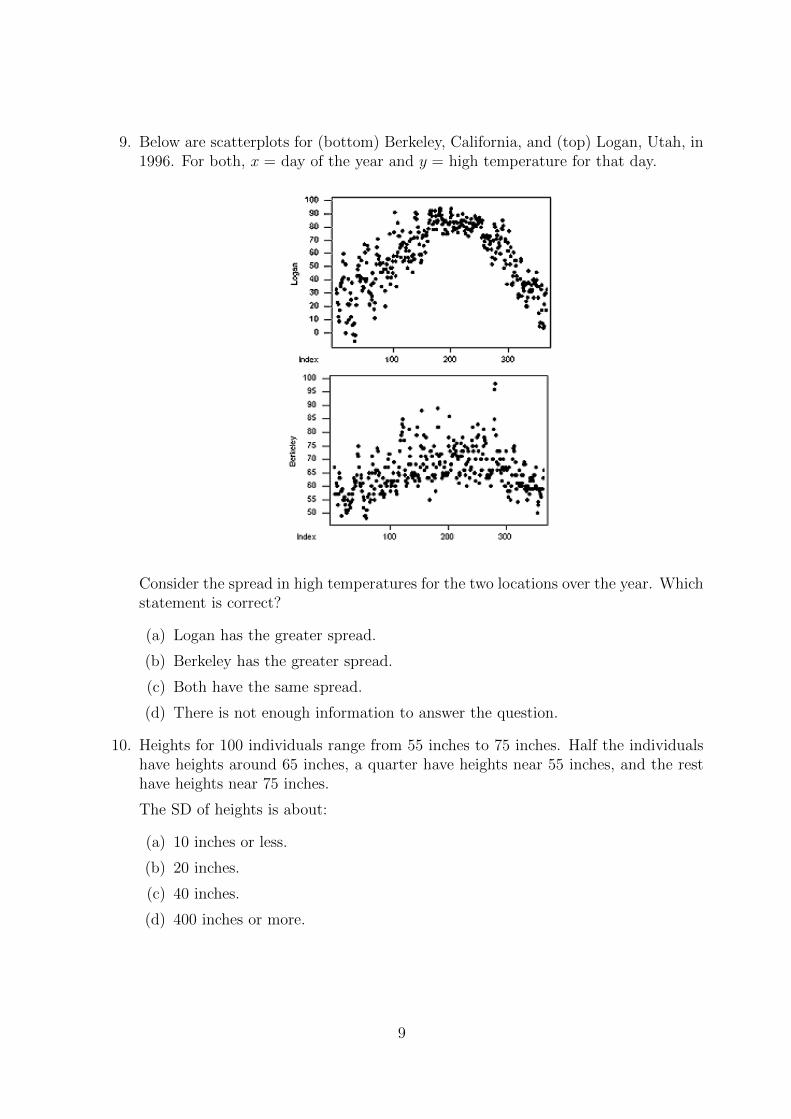
9. Below are scatterplots for (bottom) Berkeley, California, and (top) Logan, Utah, in1996. For both, x = day of the year and y = high temperature for that day.

Consider the spread in high temperatures for the two locations over the year. Whichstatement is correct?

(a) Logan has the greater spread.

(b) Berkeley has the greater spread.

(c) Both have the same spread.

(d) There is not enough information to answer the question.

10. Heights for 100 individuals range from 55 inches to 75 inches. Half the individualshave heights around 65 inches, a quarter have heights near 55 inches, and the resthave heights near 75 inches.

The SD of heights is about:

(a) 10 inches or less.

(b) 20 inches.

(c) 40 inches.

(d) 400 inches or more.

9

11. The following table is based on the numbers of children living at home, for 100statistics students:

Which histogram corresponds to the data shown in the table?

(a) Histogram A.

(b) Histogram B.

(c) Both — they are identical.

(d) None of them.

10

12. Suppose that the correlation coefficient between two variables is zero. This impliesthat

(a) there is no relationship between the two variables.

(b) there is no linear relationship between the two variables.

(c) there is no curved relationship between the two variables, but there may be alinear relationship.

(d) there are probably outliers.

11

Use the following to answer questions 13, 14, and 15:

In statistics, we usually refer to x1 as the first observation, x2 as the second obser-vation, etc., and xn as the final observation when we write down our observations inthe order they were obtained (where n represents the total number of observations).

Often, we prefer to work with data that are sorted from smallest to largest, e.g.,when calculating the median, we need the data to be sorted. Obviously, we cansimply reorder any given list of numbers. However, we often use the notation x(1)

to refer to the smallest observation, x(2) to refer to the 2nd smallest observation,etc., and x(n) to refer to the largest observation.

13. For x1 = 3, x2 = −7, x3 = −5, x4 = −2, x5 = 5, x6 = 7, and n = 6, the sum

n−1∑i=2

xi =

equals

(a) −30.

(b) −12.

(c) −9.

(d) 1.

14. For x1 = 3, x2 = −7, x3 = −5, x4 = −2, x5 = 5, x6 = 7, and n = 6, the sum

n−1∑i=2

x(i) =

equals

(a) −30.

(b) −12.

(c) −9.

(d) 1.

15. For x1 = 3, x2 = −7, x3 = −5, x4 = −2, x5 = 5, x6 = 7, and n = 6, the sum

n∑i=1

x(3) =

equals

(a) −30.

(b) −12.

(c) −9.

(d) 1.

12

T-2•

Tables

Table entry for z isthe area under thestandard normal curveto the left of z.

Probability

z

TABLE A

Standard normal probabilities

z .00 .01 .02 .03 .04 .05 .06 .07 .08 .09

−3.4 .0003 .0003 .0003 .0003 .0003 .0003 .0003 .0003 .0003 .0002−3.3 .0005 .0005 .0005 .0004 .0004 .0004 .0004 .0004 .0004 .0003−3.2 .0007 .0007 .0006 .0006 .0006 .0006 .0006 .0005 .0005 .0005−3.1 .0010 .0009 .0009 .0009 .0008 .0008 .0008 .0008 .0007 .0007−3.0 .0013 .0013 .0013 .0012 .0012 .0011 .0011 .0011 .0010 .0010−2.9 .0019 .0018 .0018 .0017 .0016 .0016 .0015 .0015 .0014 .0014−2.8 .0026 .0025 .0024 .0023 .0023 .0022 .0021 .0021 .0020 .0019−2.7 .0035 .0034 .0033 .0032 .0031 .0030 .0029 .0028 .0027 .0026−2.6 .0047 .0045 .0044 .0043 .0041 .0040 .0039 .0038 .0037 .0036−2.5 .0062 .0060 .0059 .0057 .0055 .0054 .0052 .0051 .0049 .0048−2.4 .0082 .0080 .0078 .0075 .0073 .0071 .0069 .0068 .0066 .0064−2.3 .0107 .0104 .0102 .0099 .0096 .0094 .0091 .0089 .0087 .0084−2.2 .0139 .0136 .0132 .0129 .0125 .0122 .0119 .0116 .0113 .0110−2.1 .0179 .0174 .0170 .0166 .0162 .0158 .0154 .0150 .0146 .0143−2.0 .0228 .0222 .0217 .0212 .0207 .0202 .0197 .0192 .0188 .0183−1.9 .0287 .0281 .0274 .0268 .0262 .0256 .0250 .0244 .0239 .0233−1.8 .0359 .0351 .0344 .0336 .0329 .0322 .0314 .0307 .0301 .0294−1.7 .0446 .0436 .0427 .0418 .0409 .0401 .0392 .0384 .0375 .0367−1.6 .0548 .0537 .0526 .0516 .0505 .0495 .0485 .0475 .0465 .0455−1.5 .0668 .0655 .0643 .0630 .0618 .0606 .0594 .0582 .0571 .0559−1.4 .0808 .0793 .0778 .0764 .0749 .0735 .0721 .0708 .0694 .0681−1.3 .0968 .0951 .0934 .0918 .0901 .0885 .0869 .0853 .0838 .0823−1.2 .1151 .1131 .1112 .1093 .1075 .1056 .1038 .1020 .1003 .0985−1.1 .1357 .1335 .1314 .1292 .1271 .1251 .1230 .1210 .1190 .1170−1.0 .1587 .1562 .1539 .1515 .1492 .1469 .1446 .1423 .1401 .1379−0.9 .1841 .1814 .1788 .1762 .1736 .1711 .1685 .1660 .1635 .1611−0.8 .2119 .2090 .2061 .2033 .2005 .1977 .1949 .1922 .1894 .1867−0.7 .2420 .2389 .2358 .2327 .2296 .2266 .2236 .2206 .2177 .2148−0.6 .2743 .2709 .2676 .2643 .2611 .2578 .2546 .2514 .2483 .2451−0.5 .3085 .3050 .3015 .2981 .2946 .2912 .2877 .2843 .2810 .2776−0.4 .3446 .3409 .3372 .3336 .3300 .3264 .3228 .3192 .3156 .3121−0.3 .3821 .3783 .3745 .3707 .3669 .3632 .3594 .3557 .3520 .3483−0.2 .4207 .4168 .4129 .4090 .4052 .4013 .3974 .3936 .3897 .3859−0.1 .4602 .4562 .4522 .4483 .4443 .4404 .4364 .4325 .4286 .4247

0.0 .5000 .4960 .4920 .4880 .4840 .4801 .4761 .4721 .4681 .4641

Integre Technical Publishing Co., Inc. Moore/McCabe November 16, 2007 1:29 p.m. moore page T-2

13

Tables•

T-3

Table entry for z is thearea under thestandard normal curveto the left of z.

Probability

z

TABLE A

Standard normal probabilities (continued)

z .00 .01 .02 .03 .04 .05 .06 .07 .08 .09

0.0 .5000 .5040 .5080 .5120 .5160 .5199 .5239 .5279 .5319 .53590.1 .5398 .5438 .5478 .5517 .5557 .5596 .5636 .5675 .5714 .57530.2 .5793 .5832 .5871 .5910 .5948 .5987 .6026 .6064 .6103 .61410.3 .6179 .6217 .6255 .6293 .6331 .6368 .6406 .6443 .6480 .65170.4 .6554 .6591 .6628 .6664 .6700 .6736 .6772 .6808 .6844 .68790.5 .6915 .6950 .6985 .7019 .7054 .7088 .7123 .7157 .7190 .72240.6 .7257 .7291 .7324 .7357 .7389 .7422 .7454 .7486 .7517 .75490.7 .7580 .7611 .7642 .7673 .7704 .7734 .7764 .7794 .7823 .78520.8 .7881 .7910 .7939 .7967 .7995 .8023 .8051 .8078 .8106 .81330.9 .8159 .8186 .8212 .8238 .8264 .8289 .8315 .8340 .8365 .83891.0 .8413 .8438 .8461 .8485 .8508 .8531 .8554 .8577 .8599 .86211.1 .8643 .8665 .8686 .8708 .8729 .8749 .8770 .8790 .8810 .88301.2 .8849 .8869 .8888 .8907 .8925 .8944 .8962 .8980 .8997 .90151.3 .9032 .9049 .9066 .9082 .9099 .9115 .9131 .9147 .9162 .91771.4 .9192 .9207 .9222 .9236 .9251 .9265 .9279 .9292 .9306 .93191.5 .9332 .9345 .9357 .9370 .9382 .9394 .9406 .9418 .9429 .94411.6 .9452 .9463 .9474 .9484 .9495 .9505 .9515 .9525 .9535 .95451.7 .9554 .9564 .9573 .9582 .9591 .9599 .9608 .9616 .9625 .96331.8 .9641 .9649 .9656 .9664 .9671 .9678 .9686 .9693 .9699 .97061.9 .9713 .9719 .9726 .9732 .9738 .9744 .9750 .9756 .9761 .97672.0 .9772 .9778 .9783 .9788 .9793 .9798 .9803 .9808 .9812 .98172.1 .9821 .9826 .9830 .9834 .9838 .9842 .9846 .9850 .9854 .98572.2 .9861 .9864 .9868 .9871 .9875 .9878 .9881 .9884 .9887 .98902.3 .9893 .9896 .9898 .9901 .9904 .9906 .9909 .9911 .9913 .99162.4 .9918 .9920 .9922 .9925 .9927 .9929 .9931 .9932 .9934 .99362.5 .9938 .9940 .9941 .9943 .9945 .9946 .9948 .9949 .9951 .99522.6 .9953 .9955 .9956 .9957 .9959 .9960 .9961 .9962 .9963 .99642.7 .9965 .9966 .9967 .9968 .9969 .9970 .9971 .9972 .9973 .99742.8 .9974 .9975 .9976 .9977 .9977 .9978 .9979 .9979 .9980 .99812.9 .9981 .9982 .9982 .9983 .9984 .9984 .9985 .9985 .9986 .99863.0 .9987 .9987 .9987 .9988 .9988 .9989 .9989 .9989 .9990 .99903.1 .9990 .9991 .9991 .9991 .9992 .9992 .9992 .9992 .9993 .99933.2 .9993 .9993 .9994 .9994 .9994 .9994 .9994 .9995 .9995 .99953.3 .9995 .9995 .9995 .9996 .9996 .9996 .9996 .9996 .9996 .99973.4 .9997 .9997 .9997 .9997 .9997 .9997 .9997 .9997 .9997 .9998

Integre Technical Publishing Co., Inc. Moore/McCabe November 16, 2007 1:29 p.m. moore page T-3

14