statistics for the behavioral sciences, 9th ed. use to analyze and interpret the information that...

30991_fm_ptg01_hr_i-xxii.qxd 9/3/11 12:00 AM Page ii

Licensed to:

30991_fm_ptg01_hr_i-xxii.qxd 9/3/11 12:00 AM Page ii

Copyright 2011 Cengage Learning. All Rights Reserved. May not be copied, scanned, or duplicated, in whole or in part. Due to electronic rights, some third party content may be suppressed from the eBook and/or eChapter(s).

Editorial review has deemed that any suppressed content does not materially affect the overall learning experience. Cengage Learning reserves the right to remove additional content at any time if subsequent rights restrictions require it.

This is an electronic version of the print textbook. Due to electronic rights restrictions,some third party content may be suppressed. Editorial review has deemed that any suppressed content does not materially affect the overall learning experience. The publisher reserves the right to remove content from this title at any time if subsequent rights restrictions require it. Forvaluable information on pricing, previous editions, changes to current editions, and alternate formats, please visit www.cengage.com/highered to search by ISBN#, author, title, or keyword for materials in your areas of interest.

Licensed to:

Publisher: Jon-David Hague

Psychology Editor: Tim Matray

Developmental Editor: Tangelique Williams

Freelance Developmental Editor:

Liana Sarkisian

Assistant Editor: Kelly Miller

Editorial Assistant: Lauren K. Moody

Media Editor: Mary Noel

Marketing Program Manager: Sean Foy

Marketing Communications Manager: Laura

Localio

Content Project Manager: Charlene M. Carpentier

Design Director: Rob Hugel

Art Director: Pam Galbreath

Manufacturing Planner: Judy Inouye

Rights Acquisitions Specialist: Tom McDonough

Production Service: Graphic World Inc.

Text Designer: Cheryl Carrington

Text Researcher: Karyn Morrison

Copy Editor: Graphic World Inc.

Illustrator: Graphic World Inc.

Cover Designer: Cheryl Carrington

Cover Image: Edouard Benedictus, Dover

Publications

Compositor: Graphic World Inc.

Statistics for the Behavioral Sciences,

Ninth Edition

Frederick J Gravetter and Larry B. Wallnau

© 2013, 2010 Wadsworth, Cengage Learning

ALL RIGHTS RESERVED. No part of this work covered by the copyright

herein may be reproduced, transmitted, stored, or used in any form

or by any means, graphic, electronic, or mechanical, including but not

limited to photocopying, recording, scanning, digitizing, taping, Web

distribution, information networks, or information storage and retrieval

systems, except as permitted under Section 107 or 108 of the 1976

United States Copyright Act, without the prior written permission of

the publisher.

Unless otherwise noted, all art is © Cengage Learning

Library of Congress Control Number: 2011934937

Student Edition:

ISBN-13: 978-1-111-83099-1

ISBN-10: 1-111-83099-1

Loose-leaf Edition:

ISBN-13: 978-1-111-83576-7

ISBN-10: 1-111-83576-4

Wadsworth

20 Davis Drive

Belmont, CA 94002-3098

USA

Cengage Learning is a leading provider of customized learning solutions

with office locations around the globe, including Singapore, the United

Kingdom, Australia, Mexico, Brazil, and Japan. Locate your local office at

www.cengage.com/global.

Cengage Learning products are represented in Canada by Nelson

Education, Ltd.

For your course and learning solutions, visit www.cengage.com.

Purchase any of our products at your local college store or at our

preferred online store www.CengageBrain.com.

For product information and technology assistance, contact us at

Cengage Learning Customer & Sales Support, 1-800-354-9706.

For permission to use material from this text or product,

submit all requests online at www.cengage.com/permissions.

Further permissions questions can be e-mailed to

[email protected].

Printed in the United States of America1 2 3 4 5 6 7 15 14 13 12 11

30991_fm_ptg01_hr_i-xxii.qxd 9/3/11 12:00 AM Page iv



Licensed to:

P A R T

IChapter 1 Introduction to Statistics 3

Chapter 2 Frequency Distributions 37

Chapter 3 Central Tendency 71

Chapter 4 Variability 103

We have divided this book into five sections, each cover-ing a general topic area of statistics. The first section,consisting of Chapters 1 to 4, provides a broad overview

of statistical methods and a more focused presentation of thosemethods that are classified as descriptive statistics.

By the time you finish the four chapters in this part, youshould have a good understanding of the general goals of statisticsand you should be familiar with the basic terminology and notationused in statistics. In addition, you should be familiar with the tech-niques of descriptive statistics that help researchers organize andsummarize the results they obtain from their research. Specifically,you should be able to take a set of scores and present them in atable or in a graph that provides an overall picture of the completeset. Also, you should be able to summarize a set of scores by cal-culating one or two values (such as the average) that describe theentire set.

At the end of this section there is a brief summary and a set ofreview problems that should help integrate the elements from theseparate chapters.

Introduction and DescriptiveStatistics

1

30991_ch01_ptg01_hr_001-036.qxd 9/3/11 2:05 AM Page 1



Licensed to:

Tools You Will NeedThe following items are considered essen-tial background material for this chapter. Ifyou doubt your knowledge of any of theseitems, you should review the appropriatechapter or section before proceeding.

• Proportions (math review, AppendixA)

• Fractions• Decimals• Percentages

• Basic algebra (math review, Appendix A)• z-Scores (Chapter 5)

C H A P T E R

1Introduction to Statistics

Preview

1.1 Statistics, Science, andObservations

1.2 Populations and Samples

1.3 Data Structures, ResearchMethods, and Statistics

1.4 Variables and Measurement

1.5 Statistical Notation

Summary

Focus on Problem Solving

Demonstration 1.1

Problems




Licensed to:

PreviewBefore we begin our discussion of statistics, we ask you toread the following paragraph taken from the philosophy ofWrong Shui (Candappa, 2000).

The Journey to EnlightenmentIn Wrong Shui, life is seen as a cosmic journey, a struggle to overcome unseen and unexpected obstaclesat the end of which the traveler will find illuminationand enlightenment. Replicate this quest in your homeby moving light switches away from doors and over tothe far side of each room.*

Why did we begin a statistics book with a bit of twistedphilosophy? Actually, the paragraph is an excellent (andhumorous) counterexample for the purpose of this book.Specifically, our goal is to help you avoid stumblingaround in the dark by providing lots of easily availablelight switches and plenty of illumination as you journeythrough the world of statistics. To accomplish this, we tryto present sufficient background and a clear statement ofpurpose as we introduce each new statistical procedure.Remember that all statistical procedures were developed toserve a purpose. If you understand why a new procedure isneeded, you will find it much easier to learn.

The objectives for this first chapter are to provide anintroduction to the topic of statistics and to give you somebackground for the rest of the book. We discuss the role ofstatistics within the general field of scientific inquiry, andwe introduce some of the vocabulary and notation that arenecessary for the statistical methods that follow.

As you read through the following chapters, keep inmind that the general topic of statistics follows a well-organized, logically developed progression that leads frombasic concepts and definitions to increasingly sophisticatedtechniques. Thus, the material presented in the early chap-ters of this book serves as a foundation for the material thatfollows. The content of the first nine chapters, for example,provides an essential background and context for the statis-tical methods presented in Chapter 10. If you turn directlyto Chapter 10 without reading the first nine chapters, youwill find the material confusing and incomprehensible.However, if you learn and use the background material, youwill have a good frame of reference for understanding andincorporating new concepts as they are presented.

*Candappa, R. (2000). The little book of wrong shui. Kansas City:Andrews McMeel Publishing. Reprinted by permission.

4

1.1 STATISTICS, SCIENCE, AND OBSERVATIONS

By one definition, statistics consist of facts and figures such as average income, crimerate, birth rate, baseball batting averages, and so on. These statistics are usually in-formative and time saving because they condense large quantities of information into afew simple figures. Later in this chapter we return to the notion of calculating statistics(facts and figures) but, for now, we concentrate on a much broader definition of statis-tics. Specifically, we use the term statistics to refer to a set of mathematical procedures.In this case, we are using the term statistics as a shortened version of statistical proce-dures. For example, you are probably using this book for a statistics course in whichyou will learn about the statistical techniques that are used for research in the behav-ioral sciences.

Research in psychology (and other fields) involves gathering information. To de-termine, for example, whether violence on TV has any effect on children’s behavior,you would need to gather information about children’s behaviors and the TV programsthey watch. When researchers finish the task of gathering information, they typicallyfind themselves with pages and pages of measurements such as IQ scores, personalityscores, reaction time scores, and so on. In this book, we present the statistics that

DEFINITIONS OF STATISTICS




Licensed to:

researchers use to analyze and interpret the information that they gather. Specifically,statistics serve two general purposes:

1. Statistics are used to organize and summarize the information so that the researcher can see what happened in the research study and can communicatethe results to others.

2. Statistics help the researcher to answer the questions that initiated the researchby determining exactly what general conclusions are justified based on thespecific results that were obtained.

The term statistics refers to a set of mathematical procedures for organizing,summarizing, and interpreting information.

Statistical procedures help to ensure that the information or observations are presented and interpreted in an accurate and informative way. In somewhat grandioseterms, statistics help researchers bring order out of chaos. In addition, statistics provideresearchers with a set of standardized techniques that are recognized and understoodthroughout the scientific community. Thus, the statistical methods used by one researcherare familiar to other researchers, who can accurately interpret the statistical analyses witha full understanding of how the analysis was done and what the results signify.

1.2 POPULATIONS AND SAMPLES

Research in the behavioral sciences typically begins with a general question about aspecific group (or groups) of individuals. For example, a researcher may be interestedin the effect of divorce on the self-esteem of preteen children. Or a researcher may wantto examine the amount of time spent in the bathroom for men compared to women. Inthe first example, the researcher is interested in the group of preteen children. In thesecond example, the researcher wants to compare the group of men with the group ofwomen. In statistical terminology, the entire group that a researcher wishes to study iscalled a population.

A population is the set of all the individuals of interest in a particular study.

As you can well imagine, a population can be quite large—for example, the entireset of women on the planet Earth. A researcher might be more specific, limiting thepopulation for study to women who are registered voters in the United States. Perhapsthe investigator would like to study the population consisting of women who are headsof state. Populations can obviously vary in size from extremely large to very small, de-pending on how the researcher defines the population. The population being studiedshould always be identified by the researcher. In addition, the population need not con-sist of people—it could be a population of rats, corporations, parts produced in a fac-tory, or anything else a researcher wants to study. In practice, populations are typicallyvery large, such as the population of college sophomores in the United States or thepopulation of small businesses.

Because populations tend to be very large, it usually is impossible for a researcher to examine every individual in the population of interest. Therefore, researchers typically

D E F I N I T I O N

WHAT ARE THEY?

D E F I N I T I O N

SECTION 1.2 / POPULATIONS AND SAMPLES 5




Licensed to:

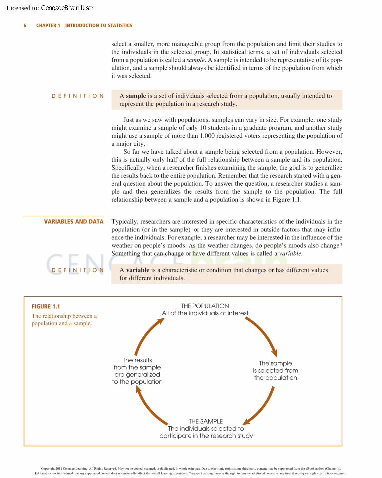
select a smaller, more manageable group from the population and limit their studies tothe individuals in the selected group. In statistical terms, a set of individuals selectedfrom a population is called a sample. A sample is intended to be representative of its pop-ulation, and a sample should always be identified in terms of the population from whichit was selected.

A sample is a set of individuals selected from a population, usually intended torepresent the population in a research study.

Just as we saw with populations, samples can vary in size. For example, one studymight examine a sample of only 10 students in a graduate program, and another studymight use a sample of more than 1,000 registered voters representing the population ofa major city.

So far we have talked about a sample being selected from a population. However,this is actually only half of the full relationship between a sample and its population.Specifically, when a researcher finishes examining the sample, the goal is to generalizethe results back to the entire population. Remember that the research started with a gen-eral question about the population. To answer the question, a researcher studies a sam-ple and then generalizes the results from the sample to the population. The fullrelationship between a sample and a population is shown in Figure 1.1.

Typically, researchers are interested in specific characteristics of the individuals in thepopulation (or in the sample), or they are interested in outside factors that may influ-ence the individuals. For example, a researcher may be interested in the influence of theweather on people’s moods. As the weather changes, do people’s moods also change?Something that can change or have different values is called a variable.

A variable is a characteristic or condition that changes or has different valuesfor different individuals.

D E F I N I T I O N

VARIABLES AND DATA

D E F I N I T I O N

6 CHAPTER 1 INTRODUCTION TO STATISTICS

THE POPULATIONAll of the individuals of interest

THE SAMPLEThe individuals selected to

participate in the research study

The resultsfrom the sampleare generalized

to the population

The sampleis selected fromthe population

FIGURE 1.1

The relationship between apopulation and a sample.




Licensed to:

Once again, variables can be characteristics that differ from one individual to another, such as height, weight, gender, or personality. Also, variables can be environ-mental conditions that change, such as temperature, time of day, or the size of the roomin which the research is being conducted.

To demonstrate changes in variables, it is necessary to make measurements of thevariables being examined. The measurement obtained for each individual is called adatum or, more commonly, a score or raw score. The complete set of scores is calledthe data set or simply the data.

Data (plural) are measurements or observations. A data set is a collection ofmeasurements or observations. A datum (singular) is a single measurement orobservation and is commonly called a score or raw score.

Before we move on, we should make one more point about samples, populations, anddata. Earlier, we defined populations and samples in terms of individuals. For example,we discussed a population of college sophomores and a sample of preschool children. Beforewarned, however, that we will also refer to populations or samples of scores. Becauseresearch typically involves measuring each individual to obtain a score, every sample (orpopulation) of individuals produces a corresponding sample (or population) of scores.

When describing data, it is necessary to distinguish whether the data come from a popu-lation or a sample. A characteristic that describes a population—for example, the averagescore for the population—is called a parameter. A characteristic that describes a sampleis called a statistic. Thus, the average score for a sample is an example of a statistic.Typically, the research process begins with a question about a population parameter.However, the actual data come from a sample and are used to compute sample statistics.

A parameter is a value, usually a numerical value, that describes a population.A parameter is usually derived from measurements of the individuals in thepopulation.

A statistic is a value, usually a numerical value, that describes a sample. Astatistic is usually derived from measurements of the individuals in the sample.

Every population parameter has a corresponding sample statistic, and most researchstudies involve using statistics from samples as the basis for answering questions aboutpopulation parameters. As a result, much of this book is concerned with the relation-ship between sample statistics and the corresponding population parameters. In Chapter7, for example, we examine the relationship between the mean obtained for a sampleand the mean for the population from which the sample was obtained.

Although researchers have developed a variety of different statistical procedures to or-ganize and interpret data, these different procedures can be classified into two generalcategories. The first category, descriptive statistics, consists of statistical proceduresthat are used to simplify and summarize data.

Descriptive statistics are statistical procedures used to summarize, organize,and simplify data.

D E F I N I T I O N

DESCRIPTIVE AND INFERENTIAL

STATISTICAL METHODS

D E F I N I T I O N S

PARAMETERS ANDSTATISTICS






Licensed to:

Descriptive statistics are techniques that take raw scores and organize or summarizethem in a form that is more manageable. Often the scores are organized in a table or agraph so that it is possible to see the entire set of scores. Another common technique isto summarize a set of scores by computing an average. Note that even if the data set hashundreds of scores, the average provides a single descriptive value for the entire set.

The second general category of statistical techniques is called inferential statistics.Inferential statistics are methods that use sample data to make general statements abouta population.

Inferential statistics consist of techniques that allow us to study samples andthen make generalizations about the populations from which they were selected.

Because populations are typically very large, it usually is not possible to measureeveryone in the population. Therefore, a sample is selected to represent the population.By analyzing the results from the sample, we hope to make general statements aboutthe population. Typically, researchers use sample statistics as the basis for drawing con-clusions about population parameters.

One problem with using samples, however, is that a sample provides only limited information about the population. Although samples are generally representative of theirpopulations, a sample is not expected to give a perfectly accurate picture of the wholepopulation. There usually is some discrepancy between a sample statistic and the corre-sponding population parameter. This discrepancy is called sampling error, and it createsthe fundamental problem that inferential statistics must always address (Box 1.1).

Sampling error is the naturally occurring discrepancy, or error, that existsbetween a sample statistic and the corresponding population parameter.

The concept of sampling error is illustrated in Figure 1.2. The figure shows a pop-ulation of 1,000 college students and two samples, each with 5 students, that have beenselected from the population. Notice that each sample contains different individualswho have different characteristics. Because the characteristics of each sample dependon the specific people in the sample, statistics vary from one sample to another. For example, the five students in sample 1 have an average age of 19.8 years and the students in sample 2 have an average age of 20.4 years.

D E F I N I T I O N

D E F I N I T I O N


B O X1.1 THE MARGIN OF ERROR BETWEEN STATISTICS AND PARAMETERS

The margin of error is the sampling error. In thiscase, the percentages that are reported were obtainedfrom a sample and are being generalized to the wholepopulation. As always, you do not expect the statisticsfrom a sample to be perfect. There is always some mar-gin of error when sample statistics are used to representpopulation parameters.

One common example of sampling error is the errorassociated with a sample proportion. For example, innewspaper articles reporting results from political polls,you frequently find statements such as this:

Candidate Brown leads the poll with 51% of thevote. Candidate Jones has 42% approval, and theremaining 7% are undecided. This poll was takenfrom a sample of registered voters and has a marginof error of plus-or-minus 4 percentage points.




Licensed to:

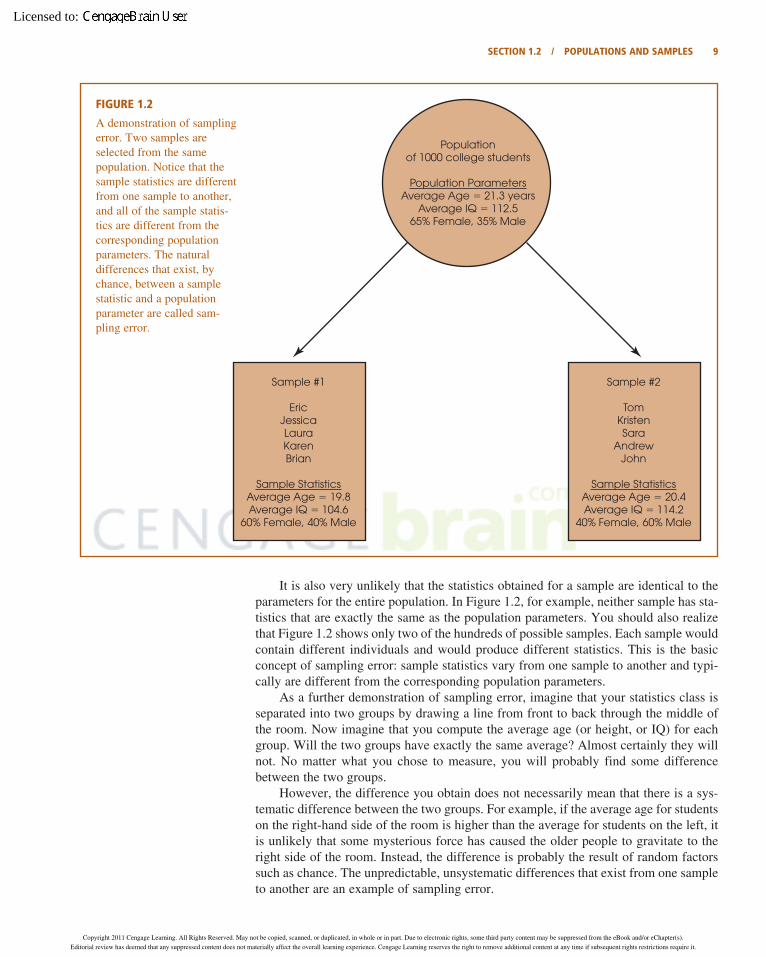
It is also very unlikely that the statistics obtained for a sample are identical to the parameters for the entire population. In Figure 1.2, for example, neither sample has sta-tistics that are exactly the same as the population parameters. You should also realizethat Figure 1.2 shows only two of the hundreds of possible samples. Each sample wouldcontain different individuals and would produce different statistics. This is the basicconcept of sampling error: sample statistics vary from one sample to another and typi-cally are different from the corresponding population parameters.

As a further demonstration of sampling error, imagine that your statistics class isseparated into two groups by drawing a line from front to back through the middle ofthe room. Now imagine that you compute the average age (or height, or IQ) for eachgroup. Will the two groups have exactly the same average? Almost certainly they willnot. No matter what you chose to measure, you will probably find some difference between the two groups.

However, the difference you obtain does not necessarily mean that there is a sys-tematic difference between the two groups. For example, if the average age for studentson the right-hand side of the room is higher than the average for students on the left, itis unlikely that some mysterious force has caused the older people to gravitate to theright side of the room. Instead, the difference is probably the result of random factorssuch as chance. The unpredictable, unsystematic differences that exist from one sampleto another are an example of sampling error.


Populationof 1000 college students

Population ParametersAverage Age � 21.3 years

Average IQ � 112.565% Female, 35% Male

Sample #1

EricJessicaLauraKarenBrian

Sample StatisticsAverage Age � 19.8Average IQ � 104.6

60% Female, 40% Male

Sample #2

TomKristenSara

AndrewJohn

Sample StatisticsAverage Age � 20.4Average IQ � 114.2

40% Female, 60% Male

FIGURE 1.2

A demonstration of samplingerror. Two samples are selected from the same population. Notice that thesample statistics are differentfrom one sample to another,and all of the sample statis-tics are different from thecorresponding populationparameters. The naturaldifferences that exist, bychance, between a samplestatistic and a populationparameter are called sam-pling error.




Licensed to:

The following example shows the general stages of a research study and demonstrateshow descriptive statistics and inferential statistics are used to organize and interpret thedata. At the end of the example, note how sampling error can affect the interpretationof experimental results, and consider why inferential statistical methods are needed todeal with this problem.

Figure 1.3 shows an overview of a general research situation and demonstrates theroles that descriptive and inferential statistics play. The purpose of the research study

E X A M P L E 1 . 1

STATISTICS IN THE CONTEXT OF RESEARCH


Step 1

Step 2

Step 3

Experiment:

Descriptive statistics:

Inferential statistics:

Compare twoteaching methods

Test scores for thestudents in eachsample

Organize and simplify

Interpret results

Sample ATaught by Method A

737672807377

757775747777

7275767674

7977787881

686775727669

7072687473

7370706970

7171717270

Sample BTaught by Method B

Sample A Sample B

Data

Averagescore = 76

Averagescore = 71

The sample data show a 5-point differencebetween the two teaching methods. However,there are two ways to interpret the results:1. There actually is no difference between the two teaching methods, and the sample difference is due to chance (sampling error).2. There really is a difference between the two methods, and the sample data accurately reflect this difference.The goal of inferential statistics is to helpresearchers decide between the two interpretations.

Population offirst-gradechildren

70 80 85 65 75 80 85

FIGURE 1.3

The role of statistics in experimental research.




Licensed to:

is to evaluate the difference between two methods for teaching reading to first-gradechildren. Two samples are selected from the population of first-grade children. Thechildren in sample A are assigned to teaching method A and the children in sample Bare assigned to method B. After 6 months, all of the students are given a standardizedreading test. At this point, the researcher has two sets of data: the scores for sample Aand the scores for sample B (see Figure 1.3). Now is the time to begin using statistics.

First, descriptive statistics are used to simplify the pages of data. For example, theresearcher could draw a graph showing the scores for each sample or compute the averagescore for each sample. Note that descriptive methods provide a simplified, organizeddescription of the scores. In this example, the students taught by method A averaged 76on the standardized test, and the students taught by method B averaged only 71.

Once the researcher has described the results, the next step is to interpret theoutcome. This is the role of inferential statistics. In this example, the researcher hasfound a difference of 5 points between the two samples (sample A averaged 76 andsample B averaged 71). The problem for inferential statistics is to differentiate between the following two interpretations:

1. There is no real difference between the two teaching methods, and the 5-pointdifference between the samples is just an example of sampling error (like thesamples in Figure 1.2).

2. There really is a difference between the two teaching methods, and the 5-pointdifference between the samples was caused by the different methods of teaching.

In simple English, does the 5-point difference between samples provide convincingevidence of a difference between the two teaching methods, or is the 5-pointdifference just chance? The purpose of inferential statistics is to answer this question.


L E A R N I N G C H E C K 1. A researcher is interested in the texting habits of high school students in theUnited States. If the researcher measures the number of text messages that each individual sends each day and calculates the average number for the entire group of high school students, the average number would be an example of a ___________.

2. A researcher is interested in how watching a reality television show featuringfashion models influences the eating behavior of 13-year-old girls.

a. A group of 30 13-year-old girls is selected to participate in a research study.The group of 30 13-year-old girls is an example of a ___________.

b. In the same study, the amount of food eaten in one day is measured for eachgirl and the researcher computes the average score for the 30 13-year-old girls.The average score is an example of a __________.

3. Statistical techniques are classified into two general categories. What are the twocategories called, and what is the general purpose for the techniques in each category?

4. Briefly define the concept of sampling error.

1. parameter

2. a. sample

b. statistic

ANSWERS




Licensed to:

1.3 DATA STRUCTURES, RESEARCH METHODS, AND STATISTICS

Some research studies are conducted simply to describe individual variables as theyexist naturally. For example, a college official may conduct a survey to describe the eat-ing, sleeping, and study habits of a group of college students. When the results consistof numerical scores, such as the number of hours spent studying each day, they are typ-ically described by the statistical techniques that are presented in Chapters 3 and 4.Non-numerical scores are typically described by computing the proportion or percent-age in each category. For example, a recent newspaper article reported that 61% of theadults in the United States currently drink alcohol.

Most research, however, is intended to examine relationships between two or morevariables. For example, is there a relationship between the amount of violence that chil-dren see on television and the amount of aggressive behavior they display? Is there arelationship between the quality of breakfast and level of academic performance for elementary school children? Is there a relationship between the number of hours ofsleep and grade point average for college students? To establish the existence of a relationship, researchers must make observations—that is, measurements of the twovariables. The resulting measurements can be classified into two distinct data structuresthat also help to classify different research methods and different statistical techniques.In the following section we identify and discuss these two data structures.

I. Measuring Two Variables for Each Individual: The Correlational MethodOne method for examining the relationship between variables is to observe the twovariables as they exist naturally for a set of individuals. That is, simply measure the twovariables for each individual. For example, research has demonstrated a relationship between sleep habits, especially wake-up time, and academic performance for college students (Trockel, Barnes, and Egget, 2000). The researchers used a survey to measurewake-up time and school records to measure academic performance for each student.Figure 1.4 shows an example of the kind of data obtained in the study. The researchersthen look for consistent patterns in the data to provide evidence for a relationship between variables. For example, as wake-up time changes from one student to another,is there also a tendency for academic performance to change?

Consistent patterns in the data are often easier to see if the scores are presented in a graph. Figure 1.4 also shows the scores for the eight students in a graph called a scatter plot. In the scatter plot, each individual is represented by a point so that the horizontal position corresponds to the student’s wake-up time and the vertical positioncorresponds to the student’s academic performance score. The scatter plot shows a clear relationship between wake-up time and academic performance: as wake-up time increases, academic performance decreases.

RELATIONSHIPS BETWEENVARIABLES

INDIVIDUAL VARIABLES


3. The two categories are descriptive statistics and inferential statistics. Descriptive techniquesare intended to organize, simplify, and summarize data. Inferential techniques use sampledata to reach general conclusions about populations.

4. Sampling error is the error, or discrepancy, between the value obtained for a sample statisticand the value for the corresponding population parameter.




Licensed to:

ABCDEFGH

1199

127

10108

StudentWake-up

Time

2.43.63.22.23.82.23.03.0

AcademicPerformance

A research study that simply measures two different variables for each individualand produces the kind of data shown in Figure 1.4 is an example of the correlationalmethod, or the correlational research strategy.

In the correlational method, two different variables are observed to determinewhether there is a relationship between them.

Limitations of the Correlational Method The results from a correlational study candemonstrate the existence of a relationship between two variables, but they do not pro-vide an explanation for the relationship. In particular, a correlational study cannotdemonstrate a cause-and-effect relationship. For example, the data in Figure 1.4 showa systematic relationship between wake-up time and academic performance for a groupof college students; those who sleep late tend to have lower performance scores thanthose who wake early. However, there are many possible explanations for the relation-ship and we do not know exactly what factor (or factors) is responsible for late sleepers having lower grades. In particular, we cannot conclude that waking students upearlier would cause their academic performance to improve, or that studying morewould cause students to wake up earlier. To demonstrate a cause-and-effect relation-ship between two variables, researchers must use the experimental method, which isdiscussed next.

II. Comparing Two (or More) Groups of Scores: Experimental andNonexperimental Methods The second method for examining the relationship between two variables involves the comparison of two or more groups of scores. In thissituation, the relationship between variables is examined by using one of the variablesto define the groups, and then measuring the second variable to obtain scores for eachgroup. For example, one group of elementary school children is shown a 30-minute action/adventure television program involving numerous instances of violence, and asecond group is shown a 30-minute comedy that includes no violence. Both groups are

D E F I N I T I O N

SECTION 1.3 / DATA STRUCTURES, RESEARCH METHODS, AND STATISTICS 13

3.8

3.6

3.4

3.2

3.0

2.8

2.6

2.4

2.2

2.0

7 8 9

Wake-up time

Ac

ad

em

ic p

erfo

rma

nc

e

10 11 12

(a) (b)

FIGURE 1.4

One of two data structures for studies evaluating therelationship between variables. Note that there are twoseparate measurements for each individual (wake-uptime and academic performance). The same scores areshown in a table (a) and in a graph (b).




Licensed to:

then observed on the playground and a researcher records the number of aggressive acts committed by each child. An example of the resulting data is shown in Figure 1.5.The researcher compares the scores for the violence group with the scores for the no-violence group. A systematic difference between the two groups provides evidencefor a relationship between viewing television violence and aggressive behavior for elementary school children.

One specific research method that involves comparing groups of scores is known as theexperimental method or the experimental research strategy. The goal of an experimen-tal study is to demonstrate a cause-and-effect relationship between two variables.Specifically, an experiment attempts to show that changing the value of one variablecauses changes to occur in the second variable. To accomplish this goal, the experi-mental method has two characteristics that differentiate experiments from other typesof research studies:

1. Manipulation The researcher manipulates one variable by changing its valuefrom one level to another. A second variable is observed (measured) to deter-mine whether the manipulation causes changes to occur.

2. Control The researcher must exercise control over the research situation toensure that other, extraneous variables do not influence the relationship beingexamined.

To demonstrate these two characteristics, consider an experiment in which researchers demonstrate the pain-killing effects of handling money (Zhou & Vohs,2009). In the experiment, a group of college students was told that they were partici-pating in a manual dexterity study. The researcher then manipulated the treatment con-ditions by giving half of the students a stack of money to count and the other half astack of blank pieces of paper. After the counting task, the participants were asked todip their hands into bowls of painfully hot water (122� F) and rate how uncomfortableit was. Participants who had counted money rated the pain significantly lower thanthose who had counted paper. The structure of the experiment is shown in Figure 1.6.

To be able to say that the difference in pain is caused by the money, the researchermust rule out any other possible explanation for the difference. That is, any other

THE EXPERIMENTAL METHOD


One variable (violence/no violence)is used to define groups

A second variable (aggressive behavior)is measured to obtain scores within each group

420132413

021300111

ViolenceNo

Violence

Compare groupsof scores

FIGURE 1.5

The second data structurefor studies evaluating therelationship between vari-ables. Note that one variableis used to define the groupsand the second variable ismeasured to obtain scoreswithin each group.

In more complex experiments, aresearcher may systematicallymanipulate more than one variable and may observe morethan one variable. Here we areconsidering the simplest case, in which only one variable ismanipulated and only one variable is observed.




Licensed to:

variables that might affect pain tolerance must be controlled. There are two general cat-egories of variables that researchers must consider:

1. Participant Variables These are characteristics such as age, gender, andintelligence that vary from one individual to another. Whenever an experimentcompares different groups of participants (one group in treatment A and a different group in treatment B), researchers must ensure that participant vari-ables do not differ from one group to another. For the experiment shown in Figure 1.6, for example, the researchers would like to conclude that handlingmoney instead of plain paper causes a change in the participants’ perceptions of pain. Suppose, however, that the participants in the money condition wereprimarily females and those in the paper condition were primarily males. In this case, there is an alternative explanation for any difference in the pain ratings that exists between the two groups. Specifically, it is possible that thedifference in pain was caused by the money, but it also is possible that thedifference was caused by the participants’ gender (females can tolerate more pain than males can). Whenever a research study allows more than oneexplanation for the results, the study is said to be confounded because it is impossible to reach an unambiguous conclusion.

2. Environmental Variables These are characteristics of the environment suchas lighting, time of day, and weather conditions. A researcher must ensure thatthe individuals in treatment A are tested in the same environment as the indi-viduals in treatment B. Using the money-counting experiment (see Figure 1.6)as an example, suppose that the individuals in the money condition were alltested in the morning and the individuals in the paper condition were all testedin the evening. Again, this would produce a confounded experiment because theresearcher could not determine whether the differences in the pain ratings werecaused by the money or caused by the time of day.

Researchers typically use three basic techniques to control other variables. First,the researcher could use random assignment, which means that each participant has anequal chance of being assigned to each of the treatment conditions. The goal of randomassignment is to distribute the participant characteristics evenly between the two groupsso that neither group is noticeably smarter (or older, or faster) than the other. Random


FIGURE 1.6

The structure of an experi-ment. Participants are ran-domly assigned to one oftwo treatment conditions:counting money or countingblank pieces of paper. Later,each participant is tested byplacing one hand in a bowlof hot (122� F) water andrating the level of pain. Adifference between theratings for the two groups isattributed to the treatment(paper versus money).

Variable #1: Counting money or blank paper (the independentvariable) Manipulated to createtwo treatment conditions.

Variable #2: Pain Rating(the dependent variable)Measured in each of thetreatment conditions.

7456686556

810

898

107887

Money Paper

Compare groupsof scores




Licensed to:

assignment can also be used to control environmental variables. For example, partici-pants could be assigned randomly for testing either in the morning or in the afternoon.Second, the researcher can use matching to ensure equivalent groups or equivalent environments. For example, the researcher could match groups by ensuring that everygroup has exactly 60% females and 40% males. Finally, the researcher can control variables by holding them constant. For example, if an experiment uses only 10-year-old children as participants (holding age constant), then the researcher can be certainthat one group is not noticeably older than another.

In the experimental method, one variable is manipulated while another vari-able is observed and measured. To establish a cause-and-effect relationshipbetween the two variables, an experiment attempts to control all other variablesto prevent them from influencing the results.

Terminology in the Experimental Method Specific names are used for the twovariables that are studied by the experimental method. The variable that is manipulatedby the experimenter is called the independent variable. It can be identified as the treat-ment conditions to which participants are assigned. For the example in Figure 1.6,money versus paper is the independent variable. The variable that is observed andmeasured to obtain scores within each condition is the dependent variable. For the example in Figure 1.6, the level of pain is the dependent variable.

The independent variable is the variable that is manipulated by the researcher.In behavioral research, the independent variable usually consists of the two (ormore) treatment conditions to which subjects are exposed. The independentvariable consists of the antecedent conditions that were manipulated prior toobserving the dependent variable.

The dependent variable is the variable that is observed to assess the effect ofthe treatment.

Control conditions in an experiment An experimental study evaluates the relation-ship between two variables by manipulating one variable (the independent variable)and measuring one variable (the dependent variable). Note that in an experiment onlyone variable is actually measured. You should realize that this is different from a cor-relational study, in which both variables are measured and the data consist of two sep-arate scores for each individual.

Often an experiment will include a condition in which the participants do not receive any treatment. The scores from these individuals are then compared with scoresfrom participants who do receive the treatment. The goal of this type of study is todemonstrate that the treatment has an effect by showing that the scores in the treatmentcondition are substantially different from the scores in the no-treatment condition. Inthis kind of research, the no-treatment condition is called the control condition, and thetreatment condition is called the experimental condition.

Individuals in a control condition do not receive the experimental treatment.Instead, they either receive no treatment or they receive a neutral, placebo treat-ment. The purpose of a control condition is to provide a baseline for compari-son with the experimental condition.

Individuals in the experimental condition do receive the experimental treatment.



D E F I N I T I O N





Licensed to:

Note that the independent variable always consists of at least two values.(Something must have at least two different values before you can say that it is “vari-able.”) For the money-counting experiment (see Figure 1.6), the independent variable ismoney versus plain paper. For an experiment with an experimental group and a controlgroup, the independent variable is treatment versus no treatment.

In informal conversation, there is a tendency for people to use the term experiment torefer to any kind of research study. You should realize, however, that the term only ap-plies to studies that satisfy the specific requirements outlined earlier. In particular, areal experiment must include manipulation of an independent variable and rigorouscontrol of other, extraneous variables. As a result, there are a number of other researchdesigns that are not true experiments but still examine the relationship between vari-ables by comparing groups of scores. Two examples are shown in Figure 1.7 and arediscussed in the following paragraphs. This type of research study is classified as non-experimental.

The top part of Figure 1.7 shows an example of a nonequivalent groups study comparing boys and girls. Notice that this study involves comparing two groups ofscores (like an experiment). However, the researcher has no ability to control which

NONEXPERIMENTALMETHODS: NONEQUIVALENT

GROUPS AND PRE–POSTSTUDIES


Variable #1: Subject gender(the quasi-independent variable)Not manipulated, but usedto create two groups of subjects

Variable #2: Verbal test scores(the dependent variable)Measured in each of thetwo groups

1719161217181516

1210141513121113

Boys Girls

Anydifference?

Variable #1: Time(the quasi-independent variable)Not manipulated, but usedto create two groups of scores

Variable #2: Depression scores(the dependent variable)Measured at each of the two different times

1719161217181516

1210141513121113

BeforeTherapy

AfterTherapy

Anydifference?

(a)

(b)

FIGURE 1.7

Two examples of nonexperi-mental studies that involvecomparing two groups ofscores. In (a) the study usestwo preexisting groups(boys/girls) and measures adependent variable (verbalscores) in each group. In (b) the study uses time (before/after) to define thetwo groups and measures a dependent variable (depres-sion) in each group.




Licensed to:

participants go into which group—all the males must be in the boy group and all the females must be in the girl group. Because this type of research compares preexistinggroups, the researcher cannot control the assignment of participants to groups and can-not ensure equivalent groups. Other examples of nonequivalent group studies includecomparing 8-year-old children and 10-year-old children, people with an eating disorderand those with no disorder, and comparing children from a single-parent home andthose from a two-parent home. Because it is impossible to use techniques like randomassignment to control participant variables and ensure equivalent groups, this type ofresearch is not a true experiment.

The bottom part of Figure 1.7 shows an example of a pre–post study comparing depression scores before therapy and after therapy. The two groups of scores are obtained by measuring the same variable (depression) twice for each participant; oncebefore therapy and again after therapy. In a pre–post study, however, the researcher hasno control over the passage of time. The “before” scores are always measured earlierthan the “after” scores. Although a difference between the two groups of scores may becaused by the treatment, it is always possible that the scores simply change as time goesby. For example, the depression scores may decrease over time in the same way that thesymptoms of a cold disappear over time. In a pre–post study, the researcher also has nocontrol over other variables that change with time. For example, the weather couldchange from dark and gloomy before therapy to bright and sunny after therapy. In thiscase, the depression scores could improve because of the weather and not because ofthe therapy. Because the researcher cannot control the passage of time or other vari-ables related to time, this study is not a true experiment.

Terminology in nonexperimental research Although the two research studiesshown in Figure 1.7 are not true experiments, you should notice that they produce thesame kind of data that are found in an experiment (see Figure 1.6). In each case, onevariable is used to create groups, and a second variable is measured to obtain scoreswithin each group. In an experiment, the groups are created by manipulation of the independent variable, and the participants’ scores are the dependent variable. The sameterminology is often used to identify the two variables in nonexperimental studies. Thatis, the variable that is used to create groups is the independent variable and the scoresare the dependent variable. For example, the top part of Figure 1.7, gender (boy/girl),is the independent variable and the verbal test scores are the dependent variable.However, you should realize that gender (boy/girl) is not a true independent variablebecause it is not manipulated. For this reason, the “independent variable” in a non-experimental study is often called a quasi-independent variable.

In a nonexperimental study, the “independent variable” that is used to create thedifferent groups of scores is often called the quasi-independent variable.

The two general data structures that we used to classify research methods can also beused to classify statistical methods.

I. One Group with Two Variables Measured for each Individual Recall that thedata from a correlational study consist of two scores, representing two different vari-ables, for each individual. The scores can be listed in a table or displayed in a scatterplot as in Figure 1.5. The relationship between the two variables is usually measuredand described using a statistic called a correlation. Correlations and the correlationalmethod are discussed in detail in Chapters15 and 16.

DATA STRUCTURES ANDSTATISTICAL METHODS

D E F I N I T I O N


Correlational studies are alsoexamples of nonexperimentalresearch. In this section, however, we are discussing non-experimental studies that compare two or more groups of scores.




Licensed to:

Occasionally, the measurement process used for a correlational study simply classi-fies individuals into categories that do not correspond to numerical values. For example,a researcher could classify a group of college students by gender (male or female) andby cell-phone preference (talk or text). Note that the researcher has two scores for eachindividual but neither of the scores is a numerical value. This type of data is typicallysummarized in a table showing how many individuals are classified into each of the pos-sible categories. Table 1.1 shows an example of this kind of summary table. The tableshows, for example, that 30 of the males in the sample preferred texting to talking. Thistype of data can be coded with numbers (for example, male � 0 and female � 1) so thatit is possible to compute a correlation. However, the relationship between variables fornon-numerical data, such as the data in Table 1.1, is usually evaluated using a statisticaltechnique known as a chi-square test. Chi-square tests are presented in Chapter 17.

II. Comparing Two or More Groups of Scores Most of the statistical procedurespresented in this book are designed for research studies that compare groups of scores,like the experimental study in Figure 1.6 and the nonexperimental studies in Figure 1.7.Specifically, we examine descriptive statistics that summarize and describe the scoresin each group, and we examine inferential statistics that allow us to use the groups, orsamples, to generalize to the entire population.

When the measurement procedure produces numerical scores, the statistical evalu-ation typically involves computing the average score for each group and then comparingthe averages. The process of computing averages is presented in Chapter 3, and a vari-ety of statistical techniques for comparing averages are presented in Chapters 8–14. If the measurement process simply classifies individuals into non-numerical categories,the statistical evaluation usually consists of computing proportions for each group andthen comparing proportions. In Table 1.1 we present an example of non-numerical dataexamining the relationship between gender and cell-phone preference. The same datacan be used to compare the proportions for males with the proportions for females. Forexample, using text is preferred by 60% of the males compared to 50% of the females. As mentioned before, these data are evaluated using a chi-square test, which ispresented in Chapter 17.

SECTION 1.4 / VARIABLES AND MEASUREMENT 19

1. Researchers have observed that high school students who watched educationaltelevision programs as young children tend to have higher grades than their peerswho did not watch educational television. Is this study an example of an experi-ment? Explain why or why not.

2. What two elements are necessary for a research study to be an experiment?

3. Loftus and Palmer (1974) conducted an experiment in which participants wereshown a video of an automobile accident. After the video, some participants were

L E A R N I N G C H E C K

TABLE 1.1

Correlational data consisting ofnon-numerical scores. Note thatthere are two measurements foreach individual: gender and cellphone preference. The numbersindicate how many people are ineach category. For example, outof the 50 males, 30 prefer textover talk.

Cell Phone Preference

Text Talk

Males 30 20 50

Females 25 25 50




Licensed to:

1.4 VARIABLES AND MEASUREMENT

The scores that make up the data from a research study are the result of observing andmeasuring variables. For example, a researcher may finish a study with a set of IQscores, personality scores, or reaction-time scores. In this section, we take a closer lookat the variables that are being measured and the process of measurement.

Some variables, such as height, weight, and eye color are well-defined, concrete enti-ties that can be observed and measured directly. On the other hand, many variablesstudied by behavioral scientists are internal characteristics that people use to help describe and explain behavior. For example, we say that a student does well in schoolbecause he or she is intelligent. Or we say that someone is anxious in social situations,or that someone seems to be hungry. Variables like intelligence, anxiety, and hungerare called constructs, and because they are intangible and cannot be directly observed,they are often called hypothetical constructs.

Although constructs such as intelligence are internal characteristics that cannot bedirectly observed, it is possible to observe and measure behaviors that are representa-tive of the construct. For example, we cannot “see” intelligence but we can see exam-ples of intelligent behavior. The external behaviors can then be used to create anoperational definition for the construct. An operational definition defines a construct interms of external behaviors that can be observed and measured. For example, your in-telligence is measured and defined by your performance on an IQ test, or hunger can bemeasured and defined by the number of hours since last eating.

Constructs are internal attributes or characteristics that cannot be directly observed but are useful for describing and explaining behavior.

An operational definition identifies a measurement procedure (a set of opera-tions) for measuring an external behavior and uses the resulting measurementsas a definition and a measurement of a hypothetical construct. Note that anoperational definition has two components: First, it describes a set of operationsfor measuring a construct. Second, it defines the construct in terms of the result-ing measurements.


CONSTRUCTS ANDOPERATIONAL DEFINITIONS


asked to estimate the speed of the cars when they “smashed into” each other.Others were asked to estimate the speed when the cars “hit” each other. The“smashed into” group produced significantly higher estimates than the “hit” group.Identify the independent and dependent variables for this study.

1. This study could be correlational or nonexperimental, but it is definitely not an example of atrue experiment. The researcher is simply observing, not manipulating, the amount of educa-tional television.

2. First, the researcher must manipulate one of the two variables being studied. Second, allother variables that might influence the results must be controlled.

3. The independent variable is the phrasing of the question and the dependent variable is thespeed estimated by each participant.

ANSWERS




Licensed to:

The variables in a study can be characterized by the type of values that can be assignedto them. A discrete variable consists of separate, indivisible categories. For this type ofvariable, there are no intermediate values between two adjacent categories. Considerthe values displayed when dice are rolled. Between neighboring values—for example,five dots and six dots—no other values can ever be observed.

A discrete variable consists of separate, indivisible categories. No values canexist between two neighboring categories.

Discrete variables are commonly restricted to whole, countable numbers—for example, the number of children in a family or the number of students attending class.If you observe class attendance from day to day, you may count 18 students one dayand 19 students the next day. However, it is impossible ever to observe a value between18 and 19. A discrete variable may also consist of observations that differ qualitatively.For example, people can be classified by gender (male or female), by occupation(nurse, teacher, lawyer, etc.), and college students can be classified by academic major(art, biology, chemistry, etc.). In each case, the variable is discrete because it consistsof separate, indivisible categories.

On the other hand, many variables are not discrete. Variables such as time, height,and weight are not limited to a fixed set of separate, indivisible categories. You canmeasure time, for example, in hours, minutes, seconds, or fractions of seconds. Thesevariables are called continuous because they can be divided into an infinite number offractional parts.

For a continuous variable, there are an infinite number of possible values thatfall between any two observed values. A continuous variable is divisible into aninfinite number of fractional parts.

Suppose, for example, that a researcher is measuring weights for a group of indi-viduals participating in a diet study. Because weight is a continuous variable, it can bepictured as a continuous line (Figure 1.8). Note that there are an infinite number of pos-sible points on the line without any gaps or separations between neighboring points. For

D E F I N I T I O N

D E F I N I T I O N

DISCRETE AND CONTINUOUSVARIABLES


149

149.5150

149.6 150.3

150.5

151 152

148.5

149

149.5

150

150.5

Real limits

151

151.5

152

152.5

FIGURE 1.8

When measuring weight tothe nearest whole pound,149.6 and 150.3 are assignedthe value of 150 (top). Anyvalue in the interval between149.5 and 150.5 is given thevalue of 150.




Licensed to:

any two different points on the line, it is always possible to find a third value that is between the two points.

Two other factors apply to continuous variables:

1. When measuring a continuous variable, it should be very rare to obtain identi-cal measurements for two different individuals. Because a continuous variablehas an infinite number of possible values, it should be almost impossible fortwo people to have exactly the same score. If the data show a substantial num-ber of tied scores, then you should suspect that the measurement procedure isvery crude or that the variable is not really continuous.

2. When measuring a continuous variable, each measurement category is actuallyan interval that must be defined by boundaries. For example, two people whoboth claim to weigh 150 pounds are probably not exactly the same weight.However, they are both around 150 pounds. One person may actually weigh149.6 and the other 150.3. Thus, a score of 150 is not a specific point on thescale but instead is an interval (see Figure 1.8). To differentiate a score of 150 from a score of 149 or 151, we must set up boundaries on the scale ofmeasurement. These boundaries are called real limits and are positioned exactlyhalfway between adjacent scores. Thus, a score of X � 150 pounds is actuallyan interval bounded by a lower real limit of 149.5 at the bottom and an upperreal limit of 150.5 at the top. Any individual whose weight falls between thesereal limits will be assigned a score of X � 150.

Real limits are the boundaries of intervals for scores that are represented on acontinuous number line. The real limit separating two adjacent scores is locatedexactly halfway between the scores. Each score has two real limits. The upperreal limit is at the top of the interval, and the lower real limit is at the bottom.

The concept of real limits applies to any measurement of a continuous variable, evenwhen the score categories are not whole numbers. For example, if you were measuringtime to the nearest tenth of a second, the measurement categories would be 31.0, 31.1, 31.2,and so on. Each of these categories represents an interval on the scale that is bounded byreal limits. For example, a score of X � 31.1 seconds indicates that the actual measurementis in an interval bounded by a lower real limit of 31.05 and an upper real limit of 31.15.Remember that the real limits are always halfway between adjacent categories.

Later in this book, real limits are used for constructing graphs and for various cal-culations with continuous scales. For now, however, you should realize that real limitsare a necessity whenever you make measurements of a continuous variable.

Finally, we should warn you that the terms continuous and discrete apply to thevariables that are being measured and not to the scores that are obtained from the meas-urement. For example, measuring people’s heights to the nearest inch produces scoresof 60, 61, 62, and so on. Although the scores may appear to be discrete numbers, theunderlying variable is continuous. One key to determining whether a variable is con-tinuous or discrete is that a continuous variable can be divided into any number of frac-tional parts. Height can be measured to the nearest inch, the nearest 0.5 inch, or thenearest 0.1 inch. Similarly, a professor evaluating students’ knowledge could use apass/fail system that classifies students into two broad categories. However, the pro-fessor could choose to use a 10-point quiz that divides student knowledge into 11 cat-egories corresponding to quiz scores from 0 to 10. Or the professor could use a100-point exam that potentially divides student knowledge into 101 categories from 0 to 100. Whenever you are free to choose the degree of precision or the number of categories for measuring a variable, the variable must be continuous.



Technical Note: Students oftenask whether a value of exactly150.5 should be assigned to theX � 150 interval or the X � 151interval. The answer is that150.5 is the boundary betweenthe two intervals and is notnecessarily in one or the other.Instead, the placement of 150.5depends on the rule that you areusing for rounding numbers. Ifyou are rounding up, then 150.5goes in the higher interval (X � 151) but if you are rounding down, then it goes inthe lower interval (X � 150).




Licensed to:

It should be obvious by now that data collection requires that we make measurements ofour observations. Measurement involves assigning individuals or events to categories. Thecategories can simply be names such as male/female or employed/unemployed, or they canbe numerical values such as 68 inches or 175 pounds. The categories used to measure avariable make up a scale of measurement, and the relationships between the categories de-termine different types of scales. The distinctions among the scales are important becausethey identify the limitations of certain types of measurements and because certain statisti-cal procedures are appropriate for scores that have been measured on some scales but noton others. If you were interested in people’s heights, for example, you could measure agroup of individuals by simply classifying them into three categories: tall, medium, andshort. However, this simple classification would not tell you much about the actual heightsof the individuals, and these measurements would not give you enough information to cal-culate an average height for the group. Although the simple classification would be ade-quate for some purposes, you would need more sophisticated measurements before youcould answer more detailed questions. In this section, we examine four different scales ofmeasurement, beginning with the simplest and moving to the most sophisticated.

The word nominal means “having to do with names.” Measurement on a nominal scaleinvolves classifying individuals into categories that have different names but are not related to each other in any systematic way. For example, if you were measuring the academic majors for a group of college students, the categories would be art, biology,business, chemistry, and so on. Each student would be classified in one category accord-ing to his or her major. The measurements from a nominal scale allow us to determinewhether two individuals are different, but they do not identify either the direction or thesize of the difference. If one student is an art major and another is a biology major we cansay that they are different, but we cannot say that art is “more than” or “less than” biol-ogy and we cannot specify how much difference there is between art and biology. Otherexamples of nominal scales include classifying people by race, gender, or occupation.

A nominal scale consists of a set of categories that have different names.Measurements on a nominal scale label and categorize observations, but do notmake any quantitative distinctions between observations.

Although the categories on a nominal scale are not quantitative values, they are occasionally represented by numbers. For example, the rooms or offices in a building maybe identified by numbers. You should realize that the room numbers are simply namesand do not reflect any quantitative information. Room 109 is not necessarily bigger thanRoom 100 and certainly not 9 points bigger. It also is fairly common to use numerical val-ues as a code for nominal categories when data are entered into computer programs. Forexample, the data from a survey may code males with a 0 and females with a 1. Again,the numerical values are simply names and do not represent any quantitative difference.The scales that follow do reflect an attempt to make quantitative distinctions.

The categories that make up an ordinal scale not only have different names (as in anominal scale) but also are organized in a fixed order corresponding to differences ofmagnitude.

An ordinal scale consists of a set of categories that are organized in an orderedsequence. Measurements on an ordinal scale rank observations in terms of sizeor magnitude.

D E F I N I T I O N

THE ORDINAL SCALE

D E F I N I T I O N

THE NOMINAL SCALE

SCALES OF MEASUREMENT





Licensed to:

Often, an ordinal scale consists of a series of ranks (first, second, third, and so on)like the order of finish in a horse race. Occasionally, the categories are identified byverbal labels like small, medium, and large drink sizes at a fast-food restaurant. In either case, the fact that the categories form an ordered sequence means that there is adirectional relationship between categories. With measurements from an ordinal scale,you can determine whether two individuals are different and you can determine the direction of difference. However, ordinal measurements do not allow you to determinethe size of the difference between two individuals. For example, if Billy is placed inthe low-reading group and Tim is placed in the high-reading group, you know that Timis a better reader, but you do not know how much better. Other examples of ordinalscales include socioeconomic class (upper, middle, lower) and T-shirt sizes (small,medium, large). In addition, ordinal scales are often used to measure variables forwhich it is difficult to assign numerical scores. For example, people can rank theirfood preferences but might have trouble explaining “how much” they prefer chocolateice cream to steak.

Both an interval scale and a ratio scale consist of a series of ordered categories (like anordinal scale) with the additional requirement that the categories form a series of inter-vals that are all exactly the same size. Thus, the scale of measurement consists of a series of equal intervals, such as inches on a ruler. Other examples of interval and ratioscales are the measurement of time in seconds, weight in pounds, and temperature indegrees Fahrenheit. Note that, in each case, one interval (1 inch, 1 second, 1 pound, 1 degree) is the same size, no matter where it is located on the scale. The fact that theintervals are all the same size makes it possible to determine both the size and the direction of the difference between two measurements. For example, you know that ameasurement of 80° Fahrenheit is higher than a measure of 60°, and you know that itis exactly 20° higher.

The factor that differentiates an interval scale from a ratio scale is the nature ofthe zero point. An interval scale has an arbitrary zero point. That is, the value 0 is assigned to a particular location on the scale simply as a matter of convenience or ref-erence. In particular, a value of zero does not indicate a total absence of the variablebeing measured. For example a temperature of 0° Fahrenheit does not mean that thereis no temperature, and it does not prohibit the temperature from going even lower.Interval scales with an arbitrary zero point are relatively rare. The two most commonexamples are the Fahrenheit and Celsius temperature scales. Other examples includegolf scores (above and below par) and relative measures such as above and below average rainfall.

A ratio scale is anchored by a zero point that is not arbitrary but rather is a mean-ingful value representing none (a complete absence) of the variable being measured.The existence of an absolute, nonarbitrary zero point means that we can measure theabsolute amount of the variable; that is, we can measure the distance from 0. Thismakes it possible to compare measurements in terms of ratios. For example, an indi-vidual who requires 10 seconds to solve a problem (10 more than 0) has taken twiceas much time as an individual who finishes in only 5 seconds (5 more than 0). Witha ratio scale, we can measure the direction and the size of the difference between twomeasurements and we can describe the difference in terms of a ratio. Ratio scales arequite common and include physical measures such as height and weight, as well asvariables such as reaction time or the number of errors on a test. The distinction between an interval scale and a ratio scale is demonstrated in Example 1.2.

THE INTERVAL AND RATIO SCALES





Licensed to:

An interval scale consists of ordered categories that are all intervals of exactlythe same size. Equal differences between numbers on a scale reflect equal differences in magnitude. However, the zero point on an interval scale is arbitrary and does not indicate a zero amount of the variable being measured.

A ratio scale is an interval scale with the additional feature of an absolute zeropoint. With a ratio scale, ratios of numbers do reflect ratios of magnitude.

A researcher obtains measurements of height for a group of 8-year-old boys. Initially, the researcher simply records each child’s height in inches, obtaining valuessuch as 44, 51, 49, and so on. These initial measurements constitute a ratio scale. Avalue of zero represents no height (absolute zero). Also, it is possible to use thesemeasurements to form ratios. For example, a child who is 60 inches tall is one-and-a-half times taller than a child who is 40 inches tall.

Now suppose that the researcher converts the initial measurement into a newscale by calculating the difference between each child’s actual height and the averageheight for this age group. A child who is 1 inch taller than average now gets a scoreof �1; a child 4 inches taller than average gets a score of �4. Similarly, a child whois 2 inches shorter than average gets a score of �2. On this scale, a score of zerocorresponds to average height. Because zero no longer indicates a complete absenceof height, the new scores constitute an interval scale of measurement.

Notice that original scores and the converted scores both involve measurement ininches, and you can compute differences, or distances, on either scale. For example,there is a 6-inch difference in height between two boys who measure 57 and 51inches tall on the first scale. Likewise, there is a 6-inch difference between two boyswho measure �9 and �3 on the second scale. However, you should also notice thatratio comparisons are not possible on the second scale. For example, a boy whomeasures �9 is not three times taller than a boy who measures �3.

For our purposes, scales of measurement are important because they influence thekind of statistics that can and cannot be used. For example, if you measure IQ scoresfor a group of students, it is possible to add the scores together and calculate a meanscore for the group. On the other hand, if you measure the academic major for eachstudent, you cannot compute the mean. (What is the mean of three psychology ma-jors, an English major, and two chemistry majors?) The vast majority of the statisti-cal techniques presented in this book are designed for numerical scores from aninterval or a ratio scale. For most statistical applications, the distinction between aninterval scale and a ratio scale is not important because both scales produce numeri-cal values that permit us to compute differences between scores, to add scores, and tocalculate mean scores. On the other hand, measurements from nominal or ordinalscales are typically not numerical values and are not compatible with many basicarithmetic operations. Therefore, alternative statistical techniques are necessary fordata from nominal or ordinal scales of measurement (for example, the median and themode in Chapter 3, the Spearman correlation in Chapter 15, and the chi-square testsin Chapter 17). Additional statistical methods for measurements from ordinal scalesare presented in Appendix E.

STATISTICS AND SCALES OF MEASUREMENT

E X A M P L E 1 . 2






Licensed to:

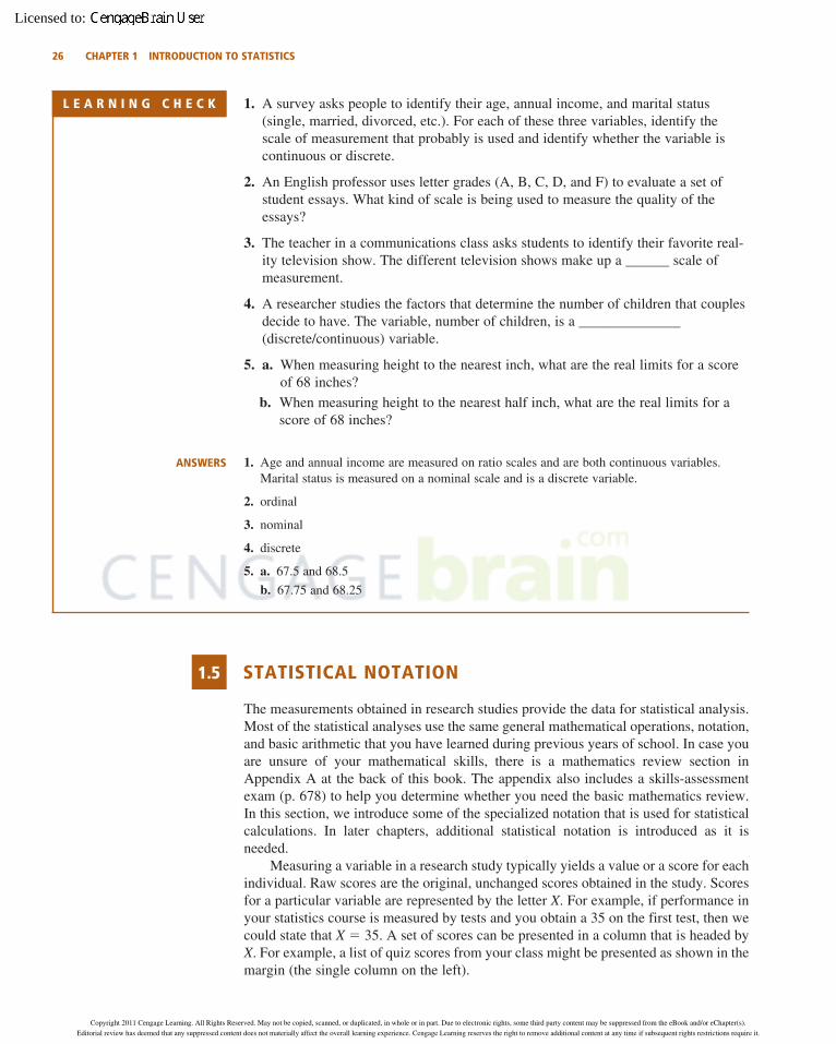
1.5 STATISTICAL NOTATION

The measurements obtained in research studies provide the data for statistical analysis.Most of the statistical analyses use the same general mathematical operations, notation,and basic arithmetic that you have learned during previous years of school. In case youare unsure of your mathematical skills, there is a mathematics review section inAppendix A at the back of this book. The appendix also includes a skills-assessmentexam (p. 678) to help you determine whether you need the basic mathematics review.In this section, we introduce some of the specialized notation that is used for statisticalcalculations. In later chapters, additional statistical notation is introduced as it isneeded.

Measuring a variable in a research study typically yields a value or a score for eachindividual. Raw scores are the original, unchanged scores obtained in the study. Scoresfor a particular variable are represented by the letter X. For example, if performance inyour statistics course is measured by tests and you obtain a 35 on the first test, then wecould state that X � 35. A set of scores can be presented in a column that is headed byX. For example, a list of quiz scores from your class might be presented as shown in themargin (the single column on the left).


L E A R N I N G C H E C K 1. A survey asks people to identify their age, annual income, and marital status (single, married, divorced, etc.). For each of these three variables, identify thescale of measurement that probably is used and identify whether the variable iscontinuous or discrete.

2. An English professor uses letter grades (A, B, C, D, and F) to evaluate a set ofstudent essays. What kind of scale is being used to measure the quality of theessays?

3. The teacher in a communications class asks students to identify their favorite real-ity television show. The different television shows make up a ______ scale ofmeasurement.

4. A researcher studies the factors that determine the number of children that couplesdecide to have. The variable, number of children, is a ______________(discrete/continuous) variable.

5. a. When measuring height to the nearest inch, what are the real limits for a scoreof 68 inches?

b. When measuring height to the nearest half inch, what are the real limits for ascore of 68 inches?

1. Age and annual income are measured on ratio scales and are both continuous variables.Marital status is measured on a nominal scale and is a discrete variable.

2. ordinal

3. nominal

4. discrete

5. a. 67.5 and 68.5

b. 67.75 and 68.25

ANSWERS




Licensed to:

When observations are made for two variables, there will be two scores for eachindividual. The data can be presented as two lists labeled X and Y for the two variables.For example, observations for people’s height in inches (variable X) and weight inpounds (variable Y) can be presented as shown in the double column in the margin.Each pair X, Y represents the observations made of a single participant.

The letter N is used to specify how many scores are in a set. An uppercase letterN identifies the number of scores in a population and a lowercase letter n identifiesthe number of scores in a sample. Throughout the remainder of the book you will notice that we often use notational differences to distinguish between samples andpopulations. For the height and weight data in the preceding table, n � 7 for bothvariables. Note that by using a lowercase letter n, we are implying that these data area sample.

Many of the computations required in statistics involve adding a set of scores. Becausethis procedure is used so frequently, a special notation is used to refer to the sum of aset of scores. The Greek letter sigma, or �, is used to stand for summation. The expression �X means to add all the scores for variable X. The summation sign, �, canbe read as “the sum of.” Thus, �X is read “the sum of the scores.” For the following setof quiz scores,

10, 6, 7, 4

�X � 27 and N � 4.

To use summation notation correctly, keep in mind the following two points:

1. The summation sign, �, is always followed by a symbol or mathematical expression. The symbol or expression identifies exactly which values are to beadded. To compute �X, for example, the symbol following the summation signis X, and the task is to find the sum of the X values. On the other hand, to compute �(X � 1)2, the summation sign is followed by a relatively complexmathematical expression, so your first task is to calculate all of the (X � 1)2

values and then add the results.

2. The summation process is often included with several other mathematical operations, such as multiplication or squaring. To obtain the correct answer, it is essential that the different operations be done in the correct sequence. Followingis a list showing the correct order of operations for performing mathematicaloperations. Most of this list should be familiar, but you should note that we haveinserted the summation process as the fourth operation in the list.

Order of Mathematical Operations

1. Any calculation contained within parentheses is done first.

2. Squaring (or raising to other exponents) is done second.

3. Multiplying and/or dividing is done third. A series of multiplication and/ordivision operations should be done in order from left to right.

4. Summation using the � notation is done next.

5. Finally, any other addition and/or subtraction is done.

The following examples demonstrate how summation notation is used in most ofthe calculations and formulas we present in this book.

SUMMATION NOTATION

SECTION 1.5 / STATISTICAL NOTATION 27

Scores

X X Y

37 72 16535 68 15135 67 16030 67 16025 68 14617 70 16016 66 133

More information on the orderof operations for mathematics isavailable in the Math Reviewappendix, page 679.




Licensed to:

A set of four scores consists of values 3, 1, 7, and 4. We will compute �X, �X2, and(�X)2 for these scores. To help demonstrate the calculations, we will use acomputational table showing the original scores (the X values) in the first column.Additional columns can then be added to show additional steps in the series ofoperations. You should notice that the first three operations in the list (parentheses,squaring, and multiplying) all create a new column of values. The last two operations,however, produce a single value corresponding to the sum.

The table to the left shows the original scores (the X values) and the squaredscores (the X2 values) that are needed to compute �X2.

The first calculation, �X, does not include any parentheses, squaring, ormultiplication, so we go directly to the summation operation. The X values are listedin the first column of the table, and we simply add the values in this column:

�X � 3 � 1 � 7 � 4 � 15

To compute �X2, the correct order of operations is to square each score and thenfind the sum of the squared values. The computational table shows the original scoresand the results obtained from squaring (the first step in the calculation). The secondstep is to find the sum of the squared values, so we simply add the numbers in the X2

column.

�X2 � 9 � 1 � 49 � 16 � 75

The final calculation, (�X)2, includes parentheses, so the first step is to performthe calculation inside the parentheses. Thus, we first find �X and then square thissum. Earlier, we computed �X � 15, so

(�X)2 � (15)2 � 225

Use the same set of four scores from Example 1.3 and compute �(X � 1) and �(X � 1)2. The following computational table will help demonstrate the calculations.

E X A M P L E 1 . 4

E X A M P L E 1 . 3


X X2

3 91 17 494 16

X (X � 1) (X � 1)2

3 2 41 0 07 6 364 3 9

The first column lists theoriginal scores. A secondcolumn lists the (X � 1)values, and a third columnshows the (X � 1)2 values.

To compute �(X � 1), the first step is to perform the operation inside the parentheses.Thus, we begin by subtracting one point from each of the X values. The resultingvalues are listed in the middle column of the table. The next step is to add the (X � 1)values.

�(X � 1) � 2 � 0 � 6 � 3 � � 11

The calculation of �(X � 1)2 requires three steps. The first step (inside parentheses)is to subtract 1 point from each X value. The results from this step are shown in themiddle column of the computational table. The second step is to square each of the




Licensed to:

(X � 1) values. The results from this step are shown in the third column of the table.The final step is to add the (X � 1)2 values to obtain

�(X � 1)2 � 4 � 0 � 36 � 9 � 49

Notice that this calculation requires squaring before adding. A common mistakeis to add the (X � 1) values and then square the total. Be careful!

In both of the preceding examples, and in many other situations, the summation operation is the last step in the calculation. According to the order of operations,parentheses, exponents, and multiplication all come before summation. However,there are situations in which extra addition and subtraction are completed after thesummation. For this example, use the same scores that appeared in the previous twoexamples, and compute �X � 1.

With no parentheses, exponents, or multiplication, the first step is the summation.Thus, we begin by computing �X. Earlier we found �X � 15. The next step is tosubtract one point from the total. For these data,

�X � 1 � 15 � 1 � 14

For this example, each individual has two scores. The first score is identified as X,and the second score is Y. With the help of the following computational table, compute �X, �Y, and �XY.

E X A M P L E 1 . 6

E X A M P L E 1 . 5

SECTION 1.5 / STATISTICAL NOTATION 29

Person X Y XY

A 3 5 15B 1 3 3C 7 4 28D 4 2 8

To find �X, simply add the values in the X column.

�X � 3 � 1 � 7 � 4 � 15

Similarly, �Y is the sum of the Y values.

�Y � 5 � 3 � 4 � 2 � 14

To compute �XY, the first step is to multiply X times Y for each individual. The resulting products (XY values) are listed in the third column of the table. Finally, we add the products to obtain

�XY � 15 � 3 � 28 � 8 � 54




Licensed to:


L E A R N I N G C H E C K 1. Calculate each value requested for the following scores: 6, 2, 4, 2.

a. �X

b. �X2

c. (�X)2

d. �(X � 2)

e. �(X � 2)2

2. Identify the first step in each of the following calculations.

a. �X2 b. (�X)2 c. �(X � 2)2

3. Use summation notation to express each of the following.

a. Add 4 points to each score and then add the resulting values.

b. Add the scores and then square the total.

c. Square each score, then add the squared values.

1. a. 14

b. 60

c. 196

d. 6

e. 20

2. a. Square each score.

b. Add the scores.

c. Subtract 2 points from each score.

3. a. �(X � 4)

b. (�X)2

c. �X2

ANSWERS

1. The term statistics is used to refer to methods fororganizing, summarizing, and interpreting data.

2. Scientific questions usually concern a population,which is the entire set of individuals one wishes tostudy. Usually, populations are so large that it isimpossible to examine every individual, so mostresearch is conducted with samples. A sample is agroup selected from a population, usually for purposesof a research study.

3. A characteristic that describes a sample is called astatistic, and a characteristic that describes a populationis called a parameter. Although sample statistics areusually representative of corresponding populationparameters, there is typically some discrepancy betweena statistic and a parameter. The naturally occurringdifference between a statistic and a parameter is calledsampling error.

4. Statistical methods can be classified into two broadcategories: descriptive statistics, which organize andsummarize data, and inferential statistics, which usesample data to draw inferences about populations.

5. The correlational method examines relationshipsbetween variables by measuring two different variablesfor each individual. This method allows researchers tomeasure and describe relationships, but cannot producea cause-and-effect explanation for the relationship.

6. The experimental method examines relationshipsbetween variables by manipulating an independentvariable to create different treatment conditions andthen measuring a dependent variable to obtain a groupof scores in each condition. The groups of scores arethen compared. A systematic difference betweengroups provides evidence that changing theindependent variable from one condition to another

SUMMARY




Licensed to:

RESOURCES 31

also caused a change in the dependent variable. Allother variables are controlled to prevent them frominfluencing the relationship. The intent of theexperimental method is to demonstrate a cause-and-effect relationship between variables.

7. Nonexperimental studies also examine relationshipsbetween variables by comparing groups of scores, butthey do not have the rigor of true experiments andcannot produce cause-and-effect explanations. Insteadof manipulating a variable to create different groups, anonexperimental study uses a preexisting participantcharacteristic (such as male/female) or the passage oftime (before/after) to create the groups being compared.

8. A measurement scale consists of a set of categoriesthat are used to classify individuals. A nominal scaleconsists of categories that differ only in name and arenot differentiated in terms of magnitude or direction. In an ordinal scale, the categories are differentiated in terms of direction, forming an ordered series. Aninterval scale consists of an ordered series ofcategories that are all equal-sized intervals. With aninterval scale, it is possible to differentiate directionand magnitude (or distance) between categories.

Finally, a ratio scale is an interval scale for which thezero point indicates none of the variable beingmeasured. With a ratio scale, ratios of measurementsreflect ratios of magnitude.

9. A discrete variable consists of indivisible categories,often whole numbers that vary in countable steps. Acontinuous variable consists of categories that areinfinitely divisible and each score corresponds to aninterval on the scale. The boundaries that separateintervals are called real limits and are located exactlyhalfway between adjacent scores.

10. The letter X is used to represent scores for a variable.If a second variable is used, Y represents its scores.The letter N is used as the symbol for the number ofscores in a population; n is the symbol for a number of scores in a sample.

11. The Greek letter sigma (�) is used to stand forsummation. Therefore, the expression �X is read “thesum of the scores.” Summation is a mathematicaloperation (like addition or multiplication) and must beperformed in its proper place in the order of operations;summation occurs after parentheses, exponents, andmultiplying/dividing have been completed.

KEY TERMS

RESOURCES

Book Companion Website: www.cengage.com/psychology/gravetterYou can find practice quizzes and other learning aids for every chapter in this book

on the book companion website, as well as a series of workshops and other resourcescorresponding to the main topic areas. In the left-hand column are a variety of learningexercises for Chapter 1, including a tutorial quiz. Also in the left-hand column, under

statistics (5)

population (5)

sample (6)

variable (6)

data (7)

data set (7)

datum (7)

raw score (7)

parameter (7)

statistic (7)

descriptive statistics (7)

inferential statistics (8)

sampling error (8)

correlational method (13)

experimental method (14)

independent variable (16)

dependent variable (16)

control condition (16)

experimental condition (16)

nonequivalent groups study (17)

pre–post study (18)

quasi-independent variable (18)

construct (20)

operational definition (20)

discrete variable (21)

continuous variable (21)

real limits (22)

upper real limit (22)

lower real limit (22)

nominal scale (23)

ordinal scale (23)

interval scale (25)

ratio scale (25)




Licensed to:

Book Resources, is a link to the workshops. For Chapter 1, there is a workshop thatreviews the scales of measurement. To get there, click on the Workshop link, then clickon Scales of Measurement. To find materials for other chapters, begin by selecting thedesired chapter at the top of the page. Note that the workshops were not developedspecifically for this book but are used by several different books written by differentauthors. As a result, you may find that some of the notation or terminology is differentfrom that which you learned in this text.

At the end of each chapter we remind you about the Web resources. Again, there isa tutorial quiz for every chapter, and we notify you whenever there is a workshop that isrelated to the chapter content.

Improve your understanding of statistics with Aplia’s auto-graded problem sets andimmediate, detailed explanations for every question. To learn more, visitwww.aplia.com/statistics.

Psychology CourseMate brings course concepts to life with interactive learning, study,and exam preparation tools that support the printed textbook. A textbook-specific web-site, Psychology CourseMate includes an integrated interactive eBook and other interac-tive learning tools including quizzes, flashcards, and more.

Visit www.cengagebrain.com to access your account and purchase materials.

The Statistical Package for the Social Sciences, known as SPSS, is a computer programthat performs most of the statistical calculations that are presented in this book, and iscommonly available on college and university computer systems. Appendix D contains ageneral introduction to SPSS. In the Resource section at the end of each chapter forwhich SPSS is applicable, there are step-by-step instructions for using SPSS to performthe statistical operations presented in the chapter.

FOCUS ON PROBLEM SOLVING

It may help to simplify summation notation if you observe that the summation sign isalways followed by a symbol or symbolic expression—for example, �X or �(X � 3). Thissymbol specifies which values you are to add. If you use the symbol as a column headingand list all the appropriate values in the column, your task is simply to add up the numbers in the column. To find �(X � 3) for example, start a column headed with (X � 3)next to the column of Xs. List all the (X � 3) values; then find the total for the column.





Licensed to:

Often, summation notation is part of a relatively complex mathematical expression thatrequires several steps of calculation. The series of steps must be performed according tothe order of mathematical operations (see page 27). The best procedure is to use a compu-tational table that begins with the original X values listed in the first column. Except forsummation, each step in the calculation creates a new column of values. For example,computing �(X � 1)2 involves three steps and produces a computational table with threecolumns. The final step is to add the values in the third column (see Example 1.4).

DEMONSTRATION 1.1

SUMMATION NOTATION

A set of scores consists of the following values:

7 3 9 5 4

For these scores, compute each of the following:

�X(�X)2

�X2

�X � 5�(X � 2)

Compute �X To compute �X, we simply add all of the scores in the group.

�X � 7 � 3 � 9 � 5 � 4 � 28

Compute (�X)2 The first step, inside the parentheses, is to compute �X. The secondstep is to square the value for �X.

�X � 28 and (�X)2 � (28)2 � 784

Compute �X2 The first step is to square each score. The second step is to add thesquared scores. The computational table shows the scores and squared scores. To compute�X2 we add the values in the X2 column.

�X2 � 49 � 9 � 81 � 25 � 16 � 180

Compute �X � 5 The first step is to compute �X. The second step is to add 5 pointsto the total.

�X � 28 and �X � 5 � 28 � 5 � 33

Compute �(X � 2) The first step, inside parentheses, is to subtract 2 points from each score. The second step is to add the resulting values. The computational table showsthe scores and the (X � 2) values. To compute �(X � 2), add the values in the (X � 2)column

�(X � 2) � 5 � 1 � 7 � 3 � 2 � 18

DEMONSTRATION 1.1 33

X X2

7 493 99 815 254 16

X X � 2

7 53 19 75 34 2




Licensed to:

PROBLEMS


*1. A researcher is investigating the effectiveness of atreatment for adolescent boys who are takingmedication for depression. A group of 30 boys isselected and half receive the new treatment in additionto their medication and the other half continue to taketheir medication without any treatment. For this study,a. Identify the population.b. Identify the sample.

2. Define the terms parameter and statistic. Be sure thatthe concepts of population and sample are included inyour definitions.

3. Statistical methods are classified into two major categories:descriptive and inferential. Describe the general purposefor the statistical methods in each category.

4. A researcher plans to compare two treatmentconditions by measuring one sample in treatment 1and a second sample in treatment 2. The researcherthen compares the scores for the two treatments andfinds a difference between the two groups.a. Briefly explain how the difference may have been

caused by the treatments.b. Briefly explain how the difference simply may be

sampling error.

5. Describe the data for a correlational research study.Explain how these data are different from the dataobtained in experimental and nonexperimental studies,which also evaluate relationships between two variables.

6. Describe how the goal of an experimental researchstudy is different from the goal for nonexperimental orcorrelational research. Identify the two elements thatare necessary for an experiment to achieve its goal.

7. Strack, Martin, and Stepper (1988) found that peoplerated cartoons as funnier when holding a pen in theirteeth (which forced them to smile) than when holdinga pen in their lips (which forced them to frown). Forthis study, identify the independent variable and thedependent variable.

8. Judge and Cable (2010) found that thin women hadhigher incomes than heavier women. Is this an exampleof an experimental or a nonexperimental study?

9. Two researchers are both interested in the relationshipbetween caffeine consumption and activity level forelementary school children. Each obtains a sample ofn � 20 children.a. The first researcher interviews each child to

determine the level of caffeine consumption. The

researcher then records the level of activity for eachchild during a 30-minute session on the playground.Is this an experimental or a nonexperimental study?Explain your answer.

b. The second researcher separates the children intotwo roughly equivalent groups. The children in onegroup are given a drink containing 300 mg ofcaffeine and the other group gets a drink with nocaffeine. The researcher then records the level ofactivity for each child during a 30-minute sessionon the playground. Is this an experimental or anonexperimental study? Explain your answer.

10. A researcher would like to evaluate the claim thatlarge doses of vitamin C can help prevent the commoncold. One group of participants is given a large dose ofthe vitamin (500 mg per day), and a second group isgiven a placebo (sugar pill). The researcher records thenumber of colds each individual experiences duringthe 3-month winter season.a. Identify the dependent variable for this study.b. Is the dependent variable discrete or continuous?c. What scale of measurement (nominal, ordinal,

interval, or ratio) is used to measure the dependentvariable?

11. A research study comparing alcohol use for collegestudents in the United States and Canada reports thatmore Canadian students drink but American studentsdrink more (Kuo, Adlaf, Lee, Gliksman, Demers, andWechsler, 2002). Is this study an example of anexperiment? Explain why or why not.

12. Oxytocin is a naturally occurring brain chemical that isnicknamed the “love hormone” because it seems toplay a role in the formation of social relationships suchas mating pairs and parent-child bonding. A recentstudy demonstrated that oxytocin appears to increasepeople’s tendency to trust others (Kosfeld, Heinrichs,Zak, Fischbacher, and Fehr, 2005). Using aninvestment game, the study demonstrated that peoplewho inhaled oxytocin were more likely to give theirmoney to a trustee compared to people who inhaled aninactive placebo. For this experimental study, identifythe independent variable and the dependent variable.

13. For each of the following, determine whether thevariable being measured is discrete or continuous and explain your answer.a. Social networking (number of daily minutes on

Facebook)b. Family size (number of siblings)

*Solutions for odd-numbered problems are provided in Appendix C.




Licensed to:

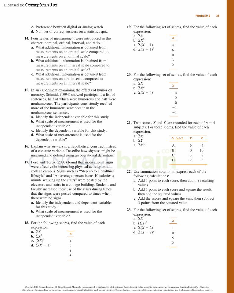
PROBLEMS 35

c. Preference between digital or analog watchd. Number of correct answers on a statistics quiz

14. Four scales of measurement were introduced in thischapter: nominal, ordinal, interval, and ratio.a. What additional information is obtained from

measurements on an ordinal scale compared tomeasurements on a nominal scale?

b. What additional information is obtained frommeasurements on an interval scale compared tomeasurements on an ordinal scale?

c. What additional information is obtained frommeasurements on a ratio scale compared tomeasurements on an interval scale?

15. In an experiment examining the effects of humor onmemory, Schmidt (1994) showed participants a list ofsentences, half of which were humorous and half werenonhumorous. The participants consistently recalledmore of the humorous sentences than thenonhumorous sentences.a. Identify the independent variable for this study.b. What scale of measurement is used for the

independent variable?c. Identify the dependent variable for this study.d. What scale of measurement is used for the

dependent variable?

16. Explain why shyness is a hypothetical construct insteadof a concrete variable. Describe how shyness might bemeasured and defined using an operational definition.

17. Ford and Torok (2008) found that motivational signswere effective in increasing physical activity on acollege campus. Signs such as “Step up to a healthierlifestyle” and “An average person burns 10 calories aminute walking up the stairs” were posted by theelevators and stairs in a college building. Students andfaculty increased their use of the stairs during timesthat the signs were posted compared to times whenthere were no signs.a. Identify the independent and dependent variables

for this study.b. What scale of measurement is used for the

independent variable?

18. For the following scores, find the value of eachexpression:a. �Xb. �X2

c. (�X)2

d. �(X � 1)

X

4215

19. For the following set of scores, find the value of eachexpression:a. �Xb. �X2

c. �(X � 1)d. �(X � 1)2

20. For the following set of scores, find the value of eachexpression:a. �Xb. �X2

c. �(X � 4)

21. Two scores, X and Y, are recorded for each of n � 4subjects. For these scores, find the value of eachexpression.a. �Xb. �Yc. �XY

22. Use summation notation to express each of thefollowing calculations:a. Add 1 point to each score, then add the resulting

values.b. Add 1 point to each score and square the result,

then add the squared values.c. Add the scores and square the sum, then subtract

3 points from the squared value.

23. For the following set of scores, find the value of eachexpression:a. �X2

b. (�X)2

c. �(X � 2)d. �(X � 2)2

X

1052

Subject X Y

A 6 4B 0 10C 3 8D 2 3

X

�4�2

0�1�1

X

46032




Licensed to:

Improve your statistical skills with

ample practice exercises and detailed

explanations on every question. Purchase

www.aplia.com/statistics




Licensed to:

REVIEW

P A R T I

133

By completing this part, you should understand and be able to perform basic descriptive statistical procedures.These include:

1. Familiarity with statistical terminology and notation(Chapter 1).

2. The ability to organize a set of scores in a frequencydistribution table or a frequency distribution graph(Chapter 2).

3. The ability to summarize and describe a distribution ofscores by computing a measure of central tendency(Chapter 3).

4. The ability to summarize and describe a distribution of scores by computing a measure of variability(Chapter 4).

The general goal of descriptive statistics is to simplify a setof data by organizing or summarizing a large set of scores.A frequency distribution table or graph organizes the entireset of scores so that it is possible to see the complete distri-bution all at once. Measures of central tendency describethe distribution by identifying its center. They also summa-rize the distribution by condensing all of the individualscores into one value that represents the entire group.Measures of variability describe whether the scores in a dis-tribution are widely scattered or closely clustered.Variability also provides an indication of how accurately ameasure of central tendency represents the entire group.

Of the basic skills presented in this part, the most com-monly used are calculating the mean and standard deviationfor a sample of numerical scores. The following exercisesshould provide an opportunity to use and reinforce thesestatistical skills.

REVIEW EXERCISES

1. a. What is the general goal for descriptive statistics?b. How is the goal served by putting scores in a fre-

quency distribution?c. How is the goal served by computing a measure of

central tendency?d. How is the goal served by computing a measure of

variability?

2. In a classic study examining the relationship betweenheredity and intelligence, Robert Tryon (1940) used aselective breeding program to develop separate strainsof “smart rats” and “dumb rats.” Tryon started with alarge sample of laboratory rats and tested each animalon a maze-learning problem. Based on their error scoresfor the maze, Tryon selected the brightest rats and thedullest rats from the sample. The brightest males weremated with the brightest females. Similarly, the dullestrats were interbred. This process of testing and selectivebreeding was continued for several generations untilTryon had established a line of maze-bright rats and aseparate line of maze-dull rats. The following data rep-resent results similar to those obtained by Tryon. Thedata consist of maze-learning error scores for the origi-nal sample of laboratory rats and the seventh generationof the maze-bright rats.

Errors Before Solving Maze

Original Rats Seventh Generation Maze-Bright Rats

10 14 7 5 8 717 13 12 8 8 611 9 20 6 10 413 6 15 6 9 84 18 10 5 7 9

13 21 6 10 8 617 11 14 9 7 8

a. Sketch a polygon showing the distribution of errorscores for the sample of original rats. On the samegraph, sketch a polygon for the sample of maze-bright rats. (Use two different colors or use adashed line for one group and a solid line for theother.) Based on the appearance of your graph, describe the differences between the two samples.

b. Calculate the mean error score for each sample.Does the mean difference support your descrip-tion from part a?

c. Calculate the variance and standard deviation foreach sample. Based on the measures of variability,is one group more diverse than the other? Is onegroup more homogeneous than the other?

30991_ch04_ptg01_hr_103-134.qxd 9/2/11 11:28 PM Page 133



statistics for the behavioral sciences, 9th ed. use to analyze and interpret the information that...

Documents