statistics of characteristic earthquakes …moho.ess.ucla.edu/~kagan/1993_bssa.pdf · statistics of...

Bulletin of the Seismological Society of America, Vol. 83, No. 1, pp. 7-24, February 1993

STATISTICS OF CHARACTERISTIC EARTHQUAKES

BY Y. Y. KAGAN

ABSTRACT

Statistical methods are used to test the characteristic earthquake hypothesis. Several distributions of earthquake size (seismic moment-frequency relations) are described. Based on the results of other researchers as well as my own tests, evidence of the characteristic earthquake hypothesis can be explained either by statistical bias or statistical artifact. Since other distributions of earthquake size provide a simpler explanation for available information, the hypothesis cannot be regarded as proven.

INTRODUCTION

Size distribution of earthquakes has important implications both for practical applications in engineering seismology (earthquake hazard analysis) and for construction of a consistent physical theory of earthquake occurrence. Since the 1940s, we have discovered (see more in Kagan, 1991) that magnitude distribution when observed over broad areas follows the Gutenberg-Richter (G-R) relation. This relation can be transformed into a power-law distribution for the scalar seismic moment. (In this note, as a measure of earthquake size, I consistently use the scalar seismic moment of an earthquake, which I denote by symbol M. Occasionally, for illustration purposes, I also use an empirical magnitude of earthquakes denoted by m.)

Considerations of finiteness of the total seismic moment or deformational energy available for an earthquake generation, and the finite size of tectonic plates, require that the power-law relation be modified at the high end of the moment scale. This upper limit is usually treated by the introduction of an additional parameter, maximum magnitude or maximum moment (McGarr, 1976; Anderson, 1979; Molnar, 1979; Anderson and Luco, 1983; Kagan, 1991). The behavior of the size distribution in the neighborhood of the maximum moment is not well known due to an insufficient number of great earthquakes in available catalogs. Although evidence exists that the moment-frequency relation bends down at the large size end of the distribution, at least, for the world wide data (see discussion in section on Earthquake Size Distribution), the data on the size distribution in particular regions are scarce. However, it is very important, especially for engineering purposes, to evaluate the maximum credi- ble size of an earthquake in a region and the probability of its occurrence. Thus, the problem can be formulated as follows: is it possible to estimate the maximum size earthquake in a region, and is its occurrence rate higher or lower than the extrapolation of the G-R relation for small and moderate shocks?

Recently a more complex model of earthquake size distribution has been proposed: the characteristic earthquake distribution (Singh et al., 1983; Wesnousky et al., 1983; Schwarz and Coppersmith, 1984; Davison and Scholz, 1985; see also Scholz, 1990). Generally, the characteristic distribution presup- poses the existence of two separate and independent earthquake populations: (1) that of regular earthquakes and (2) that of characteristic earthquakes. Regular earthquakes, which might include foreshocks and aftershocks of characteristic events, follow the G-R relation characterized by three parameters: a,

'7

8 Y . Y . KAGAN

fl, and Me, where (1) a = the number of ear thquakes in the unit of time with seismic moment higher than a cutoff level, (2) fi = the slope of the moment- frequency relation in the loglog plot, and (3) M a = the upper moment limit for regular earthquakes. The characteristic events correspond to the largest earthquakes in a region. In order to characterize these events occurrence we need at least two additional parameters: the size and the rate of occurrence of the characteristic earthquakes, Mma x and ama x.

From the point of view of general statistical and continuum-mechanical considerations, there should be no serious objection to the idea of "characteristic" earthquakes, if the hypothesis signifies tha t the distribution of ear thquakes in a region that has a particular geometry and stress pattern, may differ from the s tandard G-R relation. An ear thquake occurrence is dependent on stress distributions and geometry of faults, therefore the power-law moment-frequency law is only a first approximation. However, questions remain as to the degree of difference between the moment distribution for a large region and the distribution for a small area centered on an ear thquake fault segment, even to the form of such postulated difference. Proponents of the "characteristic earthquake" hypothesis assert tha t this difference is substantial (see Wesnousky et al., 1983, their Fig. 1) and has a particular form of sharp probability density peak at the high magnitude end of the size distribution; i.e., the frequency of these earthquakes is significantly higher than an extrapolation based on the G-R law would predict. This model is proposed on the basis of geologic evidence for similarity of large ear thquakes on fault segments, as well as on some considerations of the geometrical structure of ear thquake faults, their barriers, and the rupture process on these complex fault systems. The determination of characteristic ear thquakes for an extended fault system involves subdividing the system into individual faults and their segments. This procedure of segment selection is based on geological, seismic, and other information, and it is of a qualitative nature, since no general algorithm exists for this selection. Each of the segments is assumed to be ruptured completely by nearly identical (characteristic) earthquakes.

Recently the characteristic ear thquake hypothesis has been used to calculate the seismic risk (see, for example, Youngs and Coppersmith, 1985; Wesnousky, 1986; Nishenko, 1991) and to model ear thquake rupture propagation (Brown et al., 1991; Carlson, 1991). Because of the importance of this hypothesis it deserves rigorous testing. Kagan and Jackson (1991b) tested whether the seismic gap hypothesis predicts t ime of occurrence for large ear thquakes in the circum-Pacific seismic zones better than a random guess (the Poisson distribution) and found tha t it does not. The negative results of the gap hypothesis verification demonstrate tha t the plausible and even seemingly compelling physical and geological arguments do not guarantee tha t the hypothesis is correct. Thus, the arguments proposed for the justification of the characteristic hypothesis are not sufficient for its acceptance as a valid scientific model; the hypothesis needs to be tested and validated. This paper addresses only the subject of the size distribution of earthquakes; their temporal relations are discussed only if they are relevant for the testing of the characteristic earthquake hypothesis. Such testing encounters several difficulties:

1. The major justification for the characteristic ear thquake hypothesis comes from general geological, physical, and mechanical considerations, which are

STATISTICS OF CHARACTERISTIC EARTHQUAKES 9

of a qualitative nature and subject to various, sometimes contradictory interpretations.

2. Since the above considerations are non-unique, the quanti tat ive verification of the hypothesis is based almost exclusively upon the statistical analysis of ear thquake size distributions in various seismogenic regions (see references above).

3. Unfortunately, the seismic record in most seismic zones is too short to est imate the distribution of event sizes directly from the data. Many additional assumptions about large earthquakes, the stat ionarity of ear thquake occurrence and relation between various magnitude scales, for example, are needed before testing is possible. These assumptions make verification of results inconclusive.

4. Moreover, the characteristic hypothesis is not specified to the point where it can be subjected to a formal testing; some basic parameters of the model are known only in broad qualitative terms.

The above considerations make it almost impossible to verify or refute the characteristic hypothesis on the basis of current evidence. The best outcome we can hope to obtain is to show that the quanti tat ive proofs proposed to validate it are not sufficient; simpler models can explain available data as successfully as the characteristic hypothesis. In this paper, I do not challenge the physical, geological, and geometrical arguments tha t are used to support the characteristic hypothesis, although in the discussion section I provide some reasons that cast doubts on the possibility of objective segmentation of ear thquake faults, and therefore on the unique definition of characteristic earthquakes. However, the main point of this paper is to review the quanti tat ive statistical arguments used to verify the characteristic hypothesis. These arguments constitute a backbone for the validation of the hypothesis. In particular, the results of this paper indicate that earlier published validation at tempts contain some serious defects, at least from a statistical point of view.

Howell (1985) observes that certain statistical evidence used to prove the characteristic ear thquake hypothesis may be the result of statistical fluctuations and thus selective reporting of "successful" samples. Another possible biased selection involves, for example, taking a relatively small area around a large known ear thquake and comparing the seismicity of weak and strong ear thquakes in the area. Such a selection uses ear thquake catalog information to choose the sample that, in general, follows statistical laws that differ from a sample chosen by an unbiased procedure, jus t as the maximum member of a population has a different distribution than a randomly selected member. Thus, the catalog is used twice: first to select a sample and then to test it. As an example of such selection, suppose a fault system of length L is enclosed in a rectangle L x W. If we reduce the width W so that the largest ear thquake is kept inside the rectangle, the final sample (when W -~ 0) will contain a single earthquake.

Anderson and Luco (1983) show that many geologic and paleo-seismic studies compare ear thquake size distributions belonging to different distribution classes: those of ear thquake ruptures at a specific site and those events occurring in a specific area. It is obvious, for example, that a large ear thquake has a much higher chance to rupture the surface, thus its statistics follows a different distribution than the statistics of events tha t are registered by a seismographic

10 Y . Y . KAGAN

network (Anderson and Luco, 1983). Moreover, since these data are usually collected by different methods, their systematic errors may differ. For example, large surface ruptures are easier to discover by paleo-seismological surveys.

Comparison of seismicity levels obtained from local instrumental catalogs and from catalogs of strong ear thquakes of longer time duration is potentially an error-prone procedure. Local catalog data are usually collected over quiet peri- ods of ear thquake activity; even if a strong ear thquake occurs in an area covered by a local network, a threshold level of detection and reporting usually rises abrupt ly immediately following the main event, thus introducing a negative bias in the seismicity levels of small earthquakes. Hence, incomplete reporting of these events causes significant bias in seismicity levels. Moreover, there is substantial evidence that seismicity undergoes both short- and long-term variations (Kagan and Jackson, 1991a, and references therein). Whereas short- term changes of seismicity, due mostly to aftershock sequences, could reasonably be taken into account, no such models yet exist for the long-term variations. These variations may span decades, centuries, or even milleniums (Kagan and Jackson, 1991a).

Another source of bias is the saturat ion of all magnitude scales. This saturation is explained by the finite frequency of a seismographic network (Kagan, 1991). The saturat ion causes a loss of important information that cannot fully be restored by any transformation rule. For example, an evaluation of the recent seismicity levels by Singh e t a l . (1983) and Davison and Scholz (1985) is based on body-wave magnitude ( m b) data. m b saturates at magnitudes as low as 6.0; moreover, in order to compare m b with strong ear thquake data and fault slip data, m b is first converted into m s ; m s is, in turn, converted into the seismic moment. Clearly, significant systematic errors may accumulate during such conversions.

Since m b data are usually limited to ear thquakes of lower magnitude limits, their extrapolation to the domain of maximum events depends strongly upon accepted b values of the G-R law: even insignificant modification of the b value might bring these data into agreement with ear thquake data in the upper magnitude range. In the publications cited above, the s tandard errors in the b-value est imates have not been evaluated; these errors are significant if the total number of events in a sample (N) is small: the coefficient of variation for the b value is 1 /~N (Aki, 1965). For example, if we consider that the discrepan- cies in rates of occurrence of strong and weak ear thquakes reported in Singh e t

a l . (1983) are due to saturation, b-value uncertainties, and possible long-term fluctuations of seismicity, then only one region out of four (Oaxaca) exhibits a significant difference between extrapolated seismicity for m s events and registered "maximum" earthquakes. Such a discrepancy may readily be at t r ibuted to random fluctuations of the data (Howell, 1985).

Singh e t a l . (1983) often compare actually observed ear thquake numbers with expected numbers according to extrapolation of the G-R law. If the ratio of these numbers is high, it is considered as evidence in favor of the characteristic ear thquake hypothesis. However, if the expected number is small, the relatively high ratio values might be the result of random fluctuations. For example, for the Poisson variable with the expected value of 0.5, in 9% of cases two and more events are observed (Gnedenko, 1962, pp. 431-434). If the expected number is 1.0, there is still 1.9% probability that the actual number of events is equal to or exceeds 4. Similarly, one should not make significant conclusions when


observing two or three events in a certain magnitude interval versus zero or one event in another interval (Singh et al., 1983); such variations can be explained again by random fluctuations.

A single work among those cited escapes criticism: Davison and Scholz (1985) investigate a large portion of the circum-Pacific belt (more than 3000 km), hence there is little possibility for the selection bias or statistical fluctuations explain- ing their results. Except for use of the m b data, the s tudy analyzes a relatively homogeneous m s catalog to infer suitabili ty of the characteristic ear thquake hypothesis. Davison and Scholz (1985) first normalize m s data to the recurrence times of characteristic earthquakes; then they extrapolate the normalized seismicity levels to magnitudes of the maximum events.

For five out of nine zones where great ear thquakes occurred during this century, Davison and Scholz (1985) find that extrapolation of frequency-moment data is smaller by a factor of 10 than the moment of ear thquakes that actually originated on these segments. However, these tests are critically dependent on the est imate of the re turn t ime for the maximum magnitude events. Davison and Scholz (1985) evaluate the recurrence time by dividing the ear thquake moment by the moment accumulation rate. This procedure assumes that most elastic deformation is effected by characteristic events. However, we need to test whether another model, for example, a regular G-R relation, can explain these data with the same efficiency.

To accomplish this test, we need first to describe statistical distributions of ear thquake size. Although most of the distributions in this paper have been published earlier (see Anderson, 1979; Molnar, 1979; Anderson and Luco, 1983; Kagan, 1991), consistent use of the seismic moment allows us to simplify the formulas significantly. Thus this paper has two objectives: (1) to compile formulas for distributions of the seismic moment and related quantit ies and (2) to review available evidence and statistical tests for the characteristic ear thquake hypothesis.

EARTHQUAKE SIZE DISTRIBUTIONS

The distribution density ¢ of the seismic moment is usually assumed to follow the power-law or a Pareto distribution, which is an appropriate transformation of the G-R relation (see more in Kagan, 1991):

¢ ( M ) = f i M c ~ . M -1 ~ f o r M c < M < ~ . (1)

M c is a lower threshold seismic moment. This lower limit is introduced for two reasons: (1) since any seismographic network has a detection threshold and (2) since otherwise the distribution would diverge at M ~ 0 (there is an infinite number of events with M -~ 0). The distribution (1) requires only one degree of freedom for its characterization. In the traditional form of the G-R relation another parameter a or a (Kagan, 1991) is added; this parameter is the rate of occurrence of ear thquakes with M > M c. In later considerations, in addition to the density function, I often use the cumulative distribution function F ( M ) and the complementary function q)(M) = 1 - F ( M ) .

Statistical analysis of magnitude and seismic moment distributions yields the 1 value of fi in (1) between ~ and 1 for small and medium-size ear thquakes

(Kagan, 1991). Simple considerations of finiteness of seismic moment or deformational energy, available for an ear thquake generation, require tha t the

12 Y.Y. KAGAN

power-law relation be modified at the large size end of the moment scale. At the minimum, the distribution tail must have a decay stronger than M -1 -~ with fi > 1. This problem is generally solved by the introduction of an additional parameter, called a "maximum moment" (M~), to the distribution. This new parameterizat ion of the modified G-R relation has several forms (Anderson and Luco, 1983; Kagan, 1991). In their simplest modifications, they require at least three parameters to characterize an ear thquake occurrence.

I consider four possible distributions of ear thquake size that all satisfy the requirement of finiteness of the moment flux: (a) characteristic ear thquake distribution; (b) maximum moment distribution; (c) t runcated Pareto distribution; and (d) gamma distribution. Below I refer to cases (b), (c), and (d) as to a l t e r n a t i v e models.

In this paper the term "characteristic ear thquake distribution" refers to a distribution for which the major par t of total seismic moment flux is carried out by characteristic earthquakes, so that we essentially ignore t h e contribution of regular ear thquakes in the total budget of seismic moment rate. Thus, the seismic deformation is characterized by two parameters M~c and ax~ (moment and rate of characteristic earthquakes), which are either both evaluated inde- pendently using the available geological/seismological data or, if only one of them can be evaluated, the other can be computed from the relation

= a~cMxc, (2)

where M is the moment flux. Here I unders tand the "maximum moment distribution" as a t runcated

power-law distribution of the complementary cumulative function (Molnar, 1979)

q)(M) = for M c < M < Mxm , and (I)(M) = 0 for M ~ < M, (3)

where Mx~ is the maximum moment for this model. For the cumulative function, we obtain

M s _ Me t3 F ( M ) - M ~ for M e < M < Mxm ,

and F ( M ) = 1 forMxm < M . (4)

For the maximum moment distribution density,

Mc ]8 ~ ( M ) = f i M c ~ ' M - 1 - ~ + 6 ( M - Mxm ) •

~b(M) = 0 f o r M x m < M ,

f o r M c < = M ~ M x m ,

(5)

where 6 is the Dirac delta function. The two first distributions can be regarded as limiting cases of the general

characteristic hypothesis. In the former distribution (a), the regular earthquakes do not play a significant role in the total balance of fault slip rate and


therefore can be ignored. In the la t ter distribution (b), characteristic earthquakes are considered as an extrapolation of the regular events distribution, or as a density spike at the high moment end of the distribution. The size distributions referred to in most of the publications on characteristic earthquakes can easily be obtained as a mixture of (a) and (b).

Another model does not t runcate the complementary cumulative distribution but the density function: for the Pareto distribution t runcated on both ends (c), the distribution density is

fi M x~p • M c ~ = M-1-8 forM~ < M < M x p ,

¢ ( M ) Mx~p - M f = = (6)

where Mzp is the maximum moment for the Pareto model, which may differ fromMxm of (3). For cumulative function, we obtain

[_M__~_] ~ M~ - M f for Mc < M < Mxp, F ( M ) = Mx~p - M f = = (7)

and the complementary distribution function has a form

¢p( M) = [ _ ~ ] ~ M~p - M~ Mx~p:Mcc ~ f ° r M c < M < M x p " (s)

For the gamma distribution (d),

¢ ( M ) = C - 1 × ~ exp ~/xl f ° r M c < M < % (9a)

where Mxg is the maximum moment parameter for the gamma distribution. The parameter Mxg has a different meaning from the parameter Mxp or Mxm: whereas the lat ter two represent a "hard" limit, the former is a "soft" limit; hence in the gamma distribution some ear thquakes may have the moment M~g < M. The normalizing coefficient C is (Bateman and Erdelyi, 1953)

( ) n I Mc ~exp( Mc F(1 - fi) - ni(1---- f i + ~ , (9b) C = 1 - ~ [Mxg n~O ( - 1 ) ( M c / M x g )

where F is the gamma function. For M~ << M~g, C = 1. The cumulative function is

[ ] expl F ( M ) = C l × f i ~ [Mxg]JMo [ ~ dM

= exp 7( - f i , M / M x e) - 7( - f i , Mc/Mxg))

forM~ < M < % (10)

14 Y.Y. KAGAN

where ~ is the incomplete gamma function (Bateman and Erdelyi, 1953). The complementary distribution function has a form

¢p(M) = 1 - F ( M ) f o r M c < M < ~ . (11)

To illustrate the gamma distribution fit to actual data, Figure l a displays a cumulative histogram for the scalar seismic moment of ear thquakes in the Harvard catalog (Dziewonski et al., 1992, and references therein), for shallow earthquakes (depth interval 0 to 70 km). The available catalog covers the period from 1 Janua ry 1977 to 31 December 1991. To ensure the data uniformity events with M >__ 10177 Nm (m w >= 5.8) are used. The distribution of the worldwide data for the largest ear thquakes differs from the G-R law, but this difference has an opposite sign than the characteristic hypothesis predicts: the number of great events is smaller than the extrapolation of the G-R curve. Thus, our null hypothesis for the size distribution of the largest events should be the gamma or t runcated Pareto distribution (see below).

The maximum likelihood procedure (Kagan, 1991) allows us to retrieve the values of distribution parameters. The values of fi and Mxg are listed in Table 1 for the maximum of the likelihood function and for four extreme points of an approximate ellipse corresponding to the 95% confidence area (see Fig. 2 in Kagan, 1991). The five curves in Figure l a are calculated using the above values, they form a 95% envelope of possible approximations for the moment- frequency relation by the gamma distribution. The curves in Figure l a demonstrate that worldwide ear thquake size data are reasonably well-approximated by the gamma distribution.

For comparison, Figure lb displays the curves for the t runcated Pareto distribution (8). (We have not tried distributions (a) and (b) since they are clearly inappropriate for approximation of the worldwide data.) To obtain the values of parameters that are also listed in Table 1, I again apply the likelihood method. From (6) it is clear tha t in this case the function should reach the maximum at the M value of the largest ear thquake in the catalog ( M m a x = 3.57 • 1021 Nm), thus the maximum likelihood est imate and the lower bound of the 95% confidence area coincide. Even a visual inspection shows that the gamma distribution gives a bet ter approximation for the experimental curve. The disadvantages of the hard limit used in the t runcated Pareto distribution are more obvious if we compare the Harvard catalog with the history of the seismic moment release during the 20th century (McGarr, 1976; Kanamori, 1983). The largest ear thquake (Chilean of 1960) had a moment 2 • 1023 Nm, thus we would need to significantly modify the Mxp parameter of the Pareto distribution, whereas the gamma distribution approximates these data with only a slight change of parameters: since ear thquakes with M > Mxg are allowed in the gamma distribution, the Chilean ear thquake can be accommodated by using the "upper" curve of the 95% envelope (see Table 1).

Figure 2 displays complementary functions of distributions (3), (8), and (11) 2 (Davison and Scholz, 1985). The value of Mxm = 1023 is set, approxi- for t~ =

mately corresponding to the largest observed ear thquake in the Aleutian is- lands and Alaska (Kanamori, 1983). Other Mx's are adjusted so that the distributions would yield the same seismic moment release as (b) (see also below, equation 15). The characteristic model (a) would represent a step function in the plot at the abscissa value 1023 Nm. For the t runcated Pareto

10 4 , , , , , , , , , , , , , , , , , , , , , , , , , , , , , , , , , , , , , , , , , , , , , , , , , , , ,

Y.

E

10 3

10 2

101

l00

103

• . -.. \ ".. ,

l l l l , , i , i l l l l i H i i , l l l l , , ~ . i I . I H H 1 0 - 1 i i i i i i i i t i i i " . i i l i l t

10 17 1018 10 19 10 20 10 21 10 22 1023

10 4 , , , , , , , , , , , , , , , , , , , • , , , , , , , , , , , , , , , , , , , , , , , , , ~, , , , , , , ~

" ' ~ s i i i " . . i ; , .. i~ i ; ! i i ! ! ! ! ! ! i i i i i . "

' - , . . ~ % ,

Log Seismic Moment (Nm)

(a)

10 o

E 102 Z

7 E 10 I

~9

1 0 _ 1 , i J , , l i H

1017 , i , i l l , z t t i , , , L l l l _ t r i i t t t t ~ I ~ l l l l t i t i i L , ,

1018 1019 1020 1021 1022 1023

S T A T I S T I C S O F C H A R A C T E R I S T I C E A R T H Q U A K E S 1 5

Log Seismic Moment (Nm)

(b)

FIG. 1. L o g o f s c a l a r s e i s m i c m o m e n t v e r s u s c u m u l a t i v e f r e q u e n c y fo r t h e 1977 to 1991 H a r v a r d c a t a l o g . T h e c u r v e s s h o w t h e n u m b e r s o f s h a l l o w e a r t h q u a k e s w i t h t h e m o m e n t l a r g e r or e q u a l to M. T h e t o t a l n u m b e r o f e v e n t s w i t h M > 10177 is 2358 . D a s h e d a n d d o t t e d c u r v e s c o r r e s p o n d to t h e a p p r o x i m a t i o n b y t h e g a m m a ( l a ) a n d - P a r e t o ( l b ) d i s t r i b u t i o n s ( m a x i m u m l i k e l i h o o d s h o w n b y a d a s h e d l ine; 9 5 % e n v e l o p e s h o w n b y d o t t e d l ines) .

16 Y. Y. KAGAN

TABLE 1

PARAMETER VALUES (PARETO AND GAMMA DISTRIBUTIONS) FOR THE HARVARD CATALOG 1977-1991

L i k e l i h o o d

F u n c t i o n

_ + 9 5 % L i m i t s / 3 - v a l u e M x x 1 0 2 ] N m M x 1 0 2 1 N m / y r

Gamma distribution max 0.667 2.51 2.49 left 0.627 1.58 2.46 down 0.650 1.00 1.92 right 0.706 4.60 2.57 upper 0.683 22.0 4.65

Pareto distribution max, down 0.684 3.57 2.91 left 0.645 3.57 3.36 right 0.715 3.57 2.56 upper 0.687 11.0 4.08

10 o

10-1

, 10-2

o

1 0 -3 !

~ 1 0 4

e~

~- 1@5 o

10-6

ii

1 0 _ 7 T i I 1 . 1 . , i I I H , . , ~ i i i t l , i i i i i i i i t

1018 1019 1020 1021 1022 1 0 23 1 0 24

Seismic Moment (Nm)

FIG. 2. Complementary distribution functions for several models of earthquake size distribution: (1) Pareto distribution with unlimited maximum seismic moment (dotted line); (2) maximum moment model (solid line); (3) t runcated Pareto distribution (dashdot line); (4) gamma distribution

18 23 (dashed line). We take seismic moment cutoff at 10 Nm; M x _ = 10 ; other maximum moment is quantities are adjusted to yield the same moment rate, given num]aer of earthquakes with M > 10 :

Mxp = 3.38 x 10 -23 and Mxg = 4.74 x 1023 (see equation 15).

distribution, the return times for earthquakes with M ~ Mxp are approaching infinity since the probability of occurrence of such events obtained by integra- tion of (6) is close to zero. The gamma distribution displays similar behavior (Fig. 2).

Using this figure, one can calculate the number of expected earthquakes with the moment greater or equal to M, by multiplying the value of alp(M) by the

S T A T I S T I C S OF C H A R A C T E R I S T I C E A R T H Q U A K E S 17

total number of events with M >= M c. The difference between the alternative distributions is small for most of the moment range, only at M > 5 • 1021 the difference exceeds 10%. To distinguish between these models we need information on great earthquakes, which are extremely rare according to (c) and (d). Such events might correspond to simultaneous breaking of several segments of the subduction belt.

Using models (a) through (d) one can calculate the seismic moment release rate (moment flux), taking the seismic activity level a o for earthquakes with moment M o and greater. To avoid awkward algebra, M x >> M 0. In most cases, M 0 can be chosen to correspond to M e in (1). For the characteristic distribution the moment flux is given by (2). The total seismic moment rate according to the maximum moment distribution is (Molnar, 1979; Anderson and Luco, 1983)

1 /I//1- ~/I// f i - - " (12)

M = a o , , , x m ,,~o 1 - f i '

for the Pareto distribution we calculate (McGarr, 1976; Anderson, 1979; Ander- son and Luco, 1983)

/3 M = ~ n z l - ~ t ~ . ( 1 3 )

- 0 - , - x , - , - o 1 - 13 '

and for the gamma distribution

/3 : a°Mx~g-¢M°¢F(2 - / 3 ) 1 - - - - ~ " (14)

Table 1 displays the moment rate per year for the Harvard catalog. The estimates are relatively stable, even though the parameter values display significant variations. The rate value obtained by a direct summation of the moment is 2.33 • 1 0 21 N m / y r ; i.e,. this value is close to the values corresponding to the maximum of likelihood functions. Parenthetically I note tha t the direct summation of Kanamori (1983) data for 1921 to 1976 yields 8.53 • 1021 N m / y r , whereas McGarr (1976) found the M value of 3.4- 1022 N m / y r on the basis of plate motion calculations. Fur ther discussion of this problem is outside the scope of this article.

By equating expressions (12) to (14) for total moment rate, we can find the ratios between maximum moments in all of these distributions:

Mxg[r(2 -/3)] 1/(1-~) - - - Mxp = M x m / 3 - 1 / (1 -~ ) . (15)

2 1 For values of/3 equal to ~ or to ~ the gamma function is F(2 - 2) = 0.893 or F(2 - 1) = 0.886. Using formulas (5), (6), and (9), I calculate the distribution of 2 the total seismic moment tha t is released by an earthquake with the moment M. In this case, the distributions converge for M ~ 0, thus we do not need the truncation on the left-hand side of the distributions, and we can define the distributions on the interval 0 < M < ~. For the characteristic distribution (a), the distribution is a step function at Mxc; for other models, the total moment

18 Y . Y . KAGAN

release distributions can be calculated as

F(M) -- f jch(M)MdM. (16)

In particular, for the maximum moment distribution (b) the cumulative function is

F(M) = f l , for0<=M<__Mxm, and F = 1 forMxm < M ; (17)

for the Pareto distribution

F (3~) = , f o r 0 < M < M ~ m , and F = 1 forMxm < M ; (18)

and for the gamma distribution

1 F(]~/) - y(1 - fi, M/Mxg), for 0 < M < ~. (19)

F(1

Figure 3 displays these distributions for fi = 2 ~. The plots can be compared to similar results by Anderson and Luco (1983, their Table 1). According to all of the distributions, the major part of seismic moment release is carried out by great ear thquakes (i.e., events with ( M x / 1 0 ) < M < Mx): for case (b) it is

¢,

1 J E l l l , t l l i i i i l , l , i i i i i , l l ~ r i i i i ~ l l l

0.9

0.8

0.7

0.6

0.5

0.4

0.3

0 . 2

0.1

! /

[ /

i / };

0 . , , 1 1 1 , . ~ J i i 1 . , , , , i t , l l l l l i , , i , l , i , i , . , , , , , ~ i i , q l l

1019 1020 1 0 2 1 1 0 2 2 1 0 2 3 1 0 2 4 1 0 2 5

Seismic Moment (Nm)

FIG. 3. Distr ibution of total seismic moment released by ear thquakes with seismic moment M. The line types and values of parameters correspond to t ha t of Figure 2.


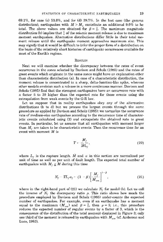
69.1%, for case (c) 53.6%, and for (d) 39.7%. In the last case (the gamma distribution), earthquakes with M > M x contribute an additional 9.6% to he total. The above values are obtained for fi = 2 ~. The maximum magnitude

1 distribution (b) implies tha t y of the seismic moment release is due to maximum moment earthquakes. Alternative distributions differ little in their total moment release until the earthquake moment approaches maximum size. This may signify tha t it would be difficult to infer the proper form of a distribution on the basis of the relatively short histories of earthquake occurrences available for most of the Earth 's regions.

RESULTS

Next we will examine whether the discrepancy between the rates of event occurrence in the zones selected by Davison and Scholz (1985) and the rates of great events which originate in the same zones might have an explanation other than characteristic distribution (a). In case of a characteristic distribution, the moment release is concentrated in a sharp, delta-function-like spike, whereas other models envision such a release in a more continuous manner. Davison and Scholz (1985) find tha t the strongest earthquakes have an occurrence rate with a factor 5 to 30 higher than the expected rate for those events using the extrapolation from weak events by the G-R law.

Let us suppose tha t in reality earthquakes obey any of the alternative distributions (b to d) but we process the largest events through the same procedure as applied by Davison and Scholz (1985): we normalize the occurrence rate of medium-size earthquakes according to the recurrence time of characteristic events calculated using (2) and extrapolate the obtained rate to great events. In particular, let us assume tha t all earthquakes with moment larger than Mf are taken to be characteristic events. Then the recurrence time for an event with moment M is

T= Mf A~IL f (20)

where Lf is the rupture length. M and a in this section are normalized per unit of time as well as per unit of fault length. The expected total number of earthquakes with Mf < M during this time

I- M r 11-~ Nr= TLfaf= ( 1 - fi)[~xm J , (21)

where in the r ight-hand part of (21) we calculate Nf for model (b). Let us call the inverse of Nf the discrepancy ratio p. This ratio shows how much the procedure employed by Davison and Scholz (1985) under-counts the expected number of earthquakes. For example, even if an earthquake has a moment equal to the maximum (Mxm) and fi = 2 y, then p = 3; i.e., this procedure reduces the expected number of regular events by a factor of 3, which is the consequence of the distribution of the total moment displayed in Figure 3; only one third of the moment is released by earthquakes with Mxm (cf. Anderson and Luco, 1983).

20 Y.Y. KAGAN

One needs to remember tha t the "true" value of M~ is unknown, so the difference obtained by using (2) is an average over possible values of M and Mx. Since we do not know the value of M~m, for model (b) I assume tha t any earthquake with Mf < M is a characteristic event. These earthquakes occur with probabilities (5), hence we calculate the average value of p as

, = fMx~p4~(M) dM = Mxm ] + - - (23)

JMr 1 - - f l Mxm ] "

For example, assuming again tha t fi = -~, and MW = 1021, which corresponds to earthquakes with m s = 8.0, we obtain ~ = 9.3. This means tha t the average discrepancy for model (b) is of one order of magnitude; i.e., it is about the same as was observed by Davison and Scholz (1985). Due to random fluctuations, this ratio may be larger or smaller for certain areas.

Similar expressions for other models can be obtained, for example, for the Pareto distribution (c)

~ = l f i 2 f i M f -1 Mxp - Mf M~p -- M--~" (24)

The values of ~ are only slightly different from tha t of (23): for the same example ~ = 9.5. Even if we taken Mf = 1022 (m s -~ 8.7), the ratio is still large --4.6.

Combined data from the Aleutian Arc (Fig. 11 in Davison and Scholz, 1985) follow one of the "noncharacteristic" alternative distributions. From a statistical point of view this is to be expected, since the data set is extensive and its selection is largely unbiased, except for the 1964 Alaskan earthquake, which was one of the two largest worldwide earthquakes in this century. Hence we should expect tha t the point corresponding to this event would be an outlier in the moment-frequency plot.

Davison and Scholz (1985) identify four out of nine zones where no strong earthquakes have occurred in this century, as potential seismic gaps. They normalize the seismicity levels measured in these zones to the re turn times of maximum moment earthquakes. These maximum events are assumed to rupture the whole extent of the appropriate segment. The arguments above are applicable to those segments of the Aleutian Arc: if the distribution of earthquake size follows model (c) or (d), we will obtain similar differences between the probabilities of the strongest events and extrapolation of seismicity, using the characteristic hypothesis (2). Parenthetically, I mention tha t during the 6 years tha t have elapsed since the publication of the Davison and Scholz' (1985) paper, strong earthquakes have not followed the seismic gap hypothesis: according to the Harvard catalog of seismic moment tensor solutions (Dziewonski et al., 1992), two earthquakes out of the six events with M > 1019"5 in the Aleutian Arc occurred in the previously identified zones (M = 1021 in 1957 zone, M = 10137 in 1938 zone), three events near, but outside the Yakataga gap, and only one (M = 1019's) occurred in the Kommandorski gap.

If we subscribe to the position tha t the size distribution of earthquakes in the Aleutian Arc follows the t runcated Pareto or gamma distribution, then we


calculate from Figure 11 in Davison and Scholz (1985) that about eight events with moment larger than 3.5 • 1021 occurred in the 85 years prior to 1985. The probability of eight ear thquakes falling into five fault zones out of a total of nine is 0.34; thus the observed ear thquake pat tern can easily be explained by a simpler assumption of the Pareto or gamma distribution.

DISCUSSION

The existence of several competing ear thquake size distributions suggests that we do not yet know the exact seismic moment-frequency relation. In general, by introducing delta-functions or sharp corners in the distributions, we impose ra ther strong constraints on the size of an earthquake. These constraints are not warranted by the available evidence, since they contradict the known behavior of dissipative physical systems. Therefore, we should introduce some degree of smoothness in the distributions which would require additional parameter(s), thus such distributions as "characteristic earthquake," "maximum moment," or the t runcated Pareto distributions will lose much appeal due to their simplicity. Only the gamma distribution satisfies both conditions: simplicity and satisfactory approximation of available data.

Although alternative distributions are similar at most of the moment range (see Fig. 2) where one has empirical evidence and all of them can be used for an approximation of moment-frequency histograms, we should be concerned with the simplicity and logical consistency of the models. For example, the characteristic ear thquake model (a) cannot by itself explain the size distribution of all ear thquakes making it necessary to invoke a general characteristic model, as discussed in the introduction. The lat ter model, in turn, requires five to six parameters for characterization, and the analysis above shows that there is no direct quanti tat ive evidence to just i fy its acceptance. Ear thquake occurrence models with three degrees of freedom approximate available data as satisfacto- rily as a general characteristic distribution. We may invoke the Ockham razor rule, thus choosing the simplest explanation and the most economical concep- tual formulation of a model.

I interpret the Ockham rule to select among models consistent with data and other available information, the model tha t has a minimum number of degrees of freedom; we should choose the model with maximum entropy, i.e., the model that, under known constraints, maximizes the uncertainty of our knowledge. In other words, unless there is compelling evidence to the contrary, we should accept the simplest distribution of ear thquake size.

In conclusion, let us examine whether the characteristic hypothesis can be effectively tested. Unless formulated as a formal quanti tat ive algorithm to specify segmentat ion of a fault zone and values of distribution parameters expected from ear thquakes occurring on these segments, it would be difficult to validate this hypothesis statistically. At present, fault segment selection is based on qualitative criteria and hence is largely subjective.

Thatcher (1990) demonstrates tha t even very large ear thquakes do not break the same segment of subduction belts; thus subdivision of a fault into segments does not assure that ear thquakes will obey these boundaries. The Working Group (1988, 1990) provided two segmentation variants of the San Francisco peninsula par t of the San Andreas fault, the Hayward, and the Rodgers Creek faults. Although the same scientists served on both panels (8 out of 12), the results of fault segmentation are significantly different (cf. Fig. 5 of the 1988

22 Y.Y. KAGAN

report and Figs. 5 and 6 of the 1990 report). As another example, Nishenko (1991) proposes a subdivision of the circum-Pacific ear thquake zone into segments that are significantly different from that of the earlier work by McCann et al. (1979).

I believe that this disagreement is not accidental: if, as accumulating evidence suggests (Kagan, 1992), the fault pat tern is scale-invariant (fractal), there are no separate scales for "individual" faults or their segments. Moreover, the fault geometry analysis (Kagan, 1992, p. 10) indicates that ear thquakes do not occur on a single (possibly wrinkled or even fractal) surface, but on a fractal s tructure of many closely correlated faults. This would indicate that we cannot meaning- fully define an individual fault surface. Thus, the objective selection of fault segments is as impossible as it is infeasible to devise a computer algorithm that would subdivide a mountain range into individual mountains or a cloudy sky into individual clouds. Suppose we try to subdivide fault pat terns as shown in Figures 10 to 12 of Tchalenko (1970) without considering the scale of the plot. In principle each segment can be subdivided further into subsegments and so on; each fault trace (surface) could again be subdivided into many quasi-parallel traces. Therefore any segmentation rule would be arbitrary, and the results obtained through such subdivision would be strongly dependent on the algo- r i thm used.

Although it is difficult to formalize the segmentation procedure, the geological insight of such studies may still yield important information on the size distribution of very large earthquakes. We cannot test this possibility statistically through a retrospective forecasting, since current segmentation models are descriptive and hence the number of degrees of freedom in the models is comparable to the number of data. However, it is possible to test the actual forecast of characteristic ear thquakes (such as made by Nishenko, 1991), where such considerations do not apply. However, in order for the prediction to be testable, it should be forecast for a large number of fault segments, so that after several years there will be a sufficient dataset to make statistically valid conclusions.

Moreover, a meaningful forecasting method must be testable against a random occurrence. Suppose an ear thquake satisfying characteristic event criteria occurs in a certain zone: it does not automatically validate the hypothesis; such an ear thquake could occur purely by chance. Thus we need to compare the forecast data set with that expected from the s tandard worldwide relation such as displayed in Figure 1. In other words, the characteristic ear thquake hypothesis, as any meaningful scientific model, must be falsifiable: accumulated evidence should either validate or reject the hypothesis.

Thus, to be verifiable, not only characteristic events have to be described completely in the forecast, but the distribution of regular ear thquakes also needs to be specified; i.e., all five or six parameters of the general characteristic distribution must be specified. At a preliminary stage, the general characteristic distribution might be defined as a worldwide generic model; thus, only one or two parameters need be adjusted for a particular fault segment. Only when it can be shown that the forecast distribution is a significantly superior approximation of the experimental data than relations (b) to (d) can we conclude that the hypothesis has been verified. Before such validation is accomplished, in practical evaluations of seismic risk a range of results should be presented to display possible alternatives. These calculations should be performed using


v a r i o u s m o d e l s of s ize d i s t r i b u t i o n w i t h i n d i c a t i o n of poss ib l e v a r i a t i o n s of

p a r a m e t e r e s t i m a t e s .

ACKNOWLEDGMENTS

I appreciate support from the National Science Foundation through Cooperative Agreement EAR-8920136 and USGS Cooperative Agreement 14-08-0001-A0899 to the Southern California Earthquake Center (SCEC). I am grateful for useful discussions held with D. Vere-Jones of Wellington University, D. D. Jackson of UCLA, and P. Bak of Brookhaven National Laboratory. I thank Associate Editor S. G. Wesnousky, reviewer P. A. Reasenberg (USGS), and an anonymous referee for their valuable remarks, which significantly improved this manuscript. Publication 5, SCEC. Publication 3808, Institute of Geophysics and Planetary Physics, University of California, Los Angeles.

REFERENCES

Aki, K. (1965). Maximum likelihood estimate of b in the formula log N = a - bM and its confidence limits, Bull. Earthquake Res. Inst. Tokyo Univ. 43, 237-239.

Anderson, J. G. (1979). Estimating the seismicity from geological structure for seismic risk studies, Bull. Seism. Soc. Am. 69, 135-158.

Anderson, J. G. and J. E. Luco (1983). Consequences of slip rate constraints on earthquake occurrence relation, Bull. Seism. Soc. Am. 73, 471-496.

Bateman, H. and A. Erdelyi (1953). Higher Transcendental Functions, McGraw-Hill, New York. Brown, S. R., C. H. Scholz, and J. B. Rundle (1991). A simplified spring-block model of earthquakes,

Geophys. Res. Lett. 18, 214-218. Carlson, J. M. (1991). Time intervals between characteristic earthquakes and correlations with

smaller events: an analysis based on a mechanical model of a fault, J. Geophys. Res. 96, 4255-4267.

Davison, F. C. and C. H. Scholz (1985). Frequency-moment distribution of earthquakes in the Aleutian Arc: a test of the characteristic earthquake model, Bull. Seism. Soc. Am. 75, 1349-1361.

Dziewonski, A. M., G. Ekstrom, M. P. Salganik, and G. Zwart (1992). Centroid-moment tensor solutions for January-March 1991, Phys. Earth Planet. Interiors 70, 7-15.

Gnedenko, B. V. (1962). The Theory of Probability, Chelsea, New York, 459 pp. Howell, B. F. (1985). On the effect of too small a data base on earthquake frequency diagrams, Bull.

Seism. Soc. Am. 75, 1205-1207. Kagan, Y. Y. (1991). Seismic moment distribution, Geophys. J. Int. 106, 123-134. Kagan, Y. Y. (1992). Seismicity: turbulence of solids, Nonlinear Sci. Today 2, 1-13. Kagan, Y. Y. and D. D. Jackson (1991a). Long-term earthquake clustering, Geophys. J. Int. 104,

117-133. Kagan, Y. Y. and D. D. Jackson (1991b). Seismic gap hypothesis: ten years after, J. Geoph. Res. 96,

21,419-21,431. Kanamori, H. (1983). Global seismicity, in Earthquakes: Observation, Theory and Interpretation,

Proc. Int. School Phys. "Enrico Fermi," Course LXXXV, H. Kanamori and E. Boschi (Editors), North Holland, Amsterdam, 596-608.

McCann, W. R., S. P. Nishenko, L. R. Sykes, and J. Krause (1979). Seismic gaps and plate tectonics: seismic potential for major boundaries, Pageoph 117, 1082-1147.

McGarr, A. (1976). Upper limit to earthquake size, Nature 262, 378-379. Molnar, P. (1979). Earthquake recurrence intervals and plate tectonics, Bull. Seism. Soc. Am. 69,

115-133. Nishenko, S. P. (1991). Circum-Pacific seismic potential: 1989-1999, Pageoph 135, 169-269. Scholz, C. H. (1990). The Mechanics of Earthquakes and Faulting, Cambridge University Press,

Cambridge. Schwarz, D. P. and K. J. Coppersmith (1984). Fault behaviour and characteristic earthquakes:

examples from Wasatch and San Andreas fault zones, J. Geophys. Res. 89, 5681-5698. Singh, S. K., M. Rodrigez, and L. Esteva (1983). Statistics of small earthquakes and frequency of

occurrence of large earthquakes along the Mexican subductien zone, Bull. Seism. Soc. Am. 73, 1779-1796.

Tchalenko, J. S. (1970). Similarities between shear zones of different magnitudes. Geol. Soc. Am. Bull. 81, 1625-1639.

24 Y, Y. KAGAN

Thatcher, W. (1990). Order and diversity in the modes of circum-Pacific earthquake recurrence, J. Geophys. Res. 95, 2609-2623.

Wesnousky, S. G. (1986). Earthquakes, Quaternary faults, and seismic hazard in California, J. Geophys. Res. 91, 12,587-12,631.

Wesnousky, S. G., C. H. Scholz, K. Shimazaki, and T. Matsuda (1983). Earthquake frequency distribution and the mechanics of faulting, J. Geophys. Res. 88, 9331-9340.

Working Group on California Earthquake Probabilities (1988). Probabilities of large earthquakes occurring in California on the San Andreas fault, U.S. Geol. Surv., Open-File rept. 88-398, 62 Pp.

Working Group on California Earthquake Probabilities (1990). Probabilities of large earthquakes in the San Francisco Bay Region, California, USGS Circular 1053, 51 pp.

Youngs, R. R. and K. J. Coppersmith (1985). Implications of fault slip rates and earthquake recurrence models to probabilistic seismic hazard estimates, Bull. Seism. Soc. Am. 75, 939-964.

Note Added in Proof--More complete discussion of the truncated Pareto distribution and evaluation of the maximum earthquake magnitude can be found in the paper by V. F. Pisarenko (1991) "Statistical evaluation of maximum possible earthquakes," Phys. Solid Earth 27, 757-763, (English translation).

INSTITUTE OF GEOPHYSICS AND PLANETARY PHYSICS UNIVERSITY OF CALIFORNIA LOS ANGELES, CALIFORNIA 90024-1567

Manuscript received 10 December 1991

statistics of characteristic earthquakes …moho.ess.ucla.edu/~kagan/1993_bssa.pdf · statistics of...

Documents