statistics of transition times, phase diffusion and

Statistics of transition times, phase diffusion andsynchronization in periodically drivenbistable systems

Peter Talkner1, Łukasz Machura1, Michael Schindler1,3,Peter Hänggi1 and Jerzy Łuczka2

1 Institut für Physik, Universität Augsburg, D-86135 Augsburg, Germany2 Institute of Physics, University of Silesia, 40-007 Katowice, PolandE-mail: [email protected]

New Journal of Physics 7 (2005) 14Received 13 September 2004Published 31 January 2005Online at http://www.njp.org/doi:10.1088/1367-2630/7/1/014

Abstract. The statistics of transitions between the metastable states of aperiodically driven bistable Brownian oscillator are investigated on the basis of atwo-state description by means of a master equation with time-dependent rates.The theoretical results are compared with extensive numerical simulations of theLangevin equation for a sinusoidal driving force.Very good agreement is achievedboth for the counting statistics of the number of transitions per period and theresidence time distribution of the process in either state. The counting statisticscorroborate in a consistent way the interpretation of stochastic resonance as asynchronization phenomenon for a properly defined generalized Rice phase.

Contents

1. Introduction 22. Rate description of a Fokker–Planck process 33. Statistics of transition times and measures of synchronization 54. Simulations 95. Discussion and conclusions 15Acknowledgments 15References 16

3 Author to whom any correspondence should be addressed.

New Journal of Physics 7 (2005) 14 PII: S1367-2630(05)86413-41367-2630/05/010014+16$30.00 © IOP Publishing Ltd and Deutsche Physikalische Gesellschaft

mailto:[email protected]

http://www.njp.org/

2 DEUTSCHE PHYSIKALISCHE GESELLSCHAFT

1. Introduction

Time-dependent systems that are in contact with an environment represent an important classof non-equilibrium systems. In these systems effects may be observed that cannot occur inthermal equilibrium, as for example noise-sustained signal amplification by means of stochasticresonance [1], or the rectification of noise and the appearance of directed transport in ratchet-like systems [2]. In the case of stochastic resonance the transitions between two metastablestates appear to be synchronized with an external, often periodic signal that acts as a forcingon the considered system [3, 4]. This force alone, however, may be much too small to drive thesystem from one state to the other. Responsible for the occurrence of transitions are randomforces imposed by the environment in the form of thermal noise. These kinds of processes canconveniently be modelled by means of Langevin equations which are the equations of motionfor the relevant degree (or degrees) of freedom of the considered system and which comprise theinfluence of the environment in the form of dissipative and random forces [5]. Unfortunately,neither the Langevin equations nor the equivalent Fokker–Planck equations for the time evolutionof the system’s probability density can be solved analytically for other than a few rather specialsituations [6]. Therefore, most of the prior investigations of stochastic resonance are based onthe numerical simulation of Langevin equations [1], or the numerical solution of Fokker–Planckequations either by means of continued fractions [7] or Galerkin-type approximation schemes[8, 9]. Analytical results have been obtained in limiting cases, such as weak driving forces [1],or weak noise [8].

Interestingly enough, the same qualitative features that had been known from numericalinvestigations also resulted from very simple discrete models [10, 11] that contain only twostates representing the metastable states of the continuous model. The dynamics of the discretestates is Markovian and therefore governed by a master equation. The external driving results ina time-dependent modulation of the transition rates of this master equation. In a recent work [12]it was shown that such master equations correctly describe the relevant aspects of the long-timedynamics of continuously driven systems with metastable states provided that the intra-welldynamics is fast compared to both the driving and the noise-activated transitions between themetastable states.

In the present work we will pursue ideas [4] suggesting that a periodically driven bistablesystem can be characterized in terms of a conveniently defined phase that may be locked withthe phase of the external force, yielding in this way a more precise notion of synchronizationfor such systems. Various possible definitions of phases for a bistable Brownian oscillator havebeen compared in [4] with the main result that the precise definition does not matter much inthe rate-limited regime where the master equation applies. Therefore, one will use the definitionfor which it is simplest to determine the corresponding phase. If we think of the system as ofa particle moving in a bistable potential under the influence of a stochastic and a driving forcethen the Rice phase provides a convenient definition under the condition that the particle has acontinuous velocity [4, 13]. This phase counts the number of crossings of the potential maximumseparating the two wells. The necessary continuity of the velocity is guaranteed if the hypotheticalparticle has a mass and obeys a Newtonian equation of motion. The continuity of the velocity islost if the particle is overdamped and described by an ‘Aristotelian equation of motion,’ i.e. by afirst-order differential equation for the position driven by a Gaussian white stochastic force. Thenthe trajectories are known to be nowhere differentiable and to possess further level crossings inthe close temporal neighbourhood of each single one.

New Journal of Physics 7 (2005) 14 (http://www.njp.org/)

http://www.njp.org/


We will allow for this jittering character of Brownian trajectories by setting two differentthresholds on both sides of the potential maximum and only count alternating crossings. Bydefinition, the generalized Rice phase increases by π upon each counted crossing of eitherthreshold. We will choose the threshold positions in such a way that an immediate recrossingof the barrier from either threshold is highly unlikely. Put differently, up to exceptional cases,the particle will move from the threshold to the adjacent well rather than immediately jumpback over the barrier to the original well. In the two-state description of the process, we canthen identify the phase by counting the number of transitions between the two states. With eachtransition the phase grows by π. In a previous work [14], one of us gave explicit expressionsfor various quantities characterizing the alternating point process, comprised of the entrancetimes into the states of a Markovian two-state process with periodic time-dependent rates. Thedefinition of the Rice phase in that work was based on the statistics of the entrance times intoone particular state. Some of the statistical details then depend on the choice of this state. Toavoid this ambiguity we here base our definition on the transitions between both states.

A further quantity that has been introduced in order to characterize stochastic resonance isthe distribution of residence times [15]. It is also based on the statistics of the transition timesand characterizes the duration between two neighbouring transitions.

The paper is organized as follows. In section 2 we introduce the model, formulate therespective equivalent Langevin and Fokker–Planck equations and give the formal solutions ofthe two-state Markov process with time-dependent rates that follow from the Fokker–Planckequation. In section 3 several statistical tools from the theory of point processes are introduced bymeans of which the switching behaviour resulting from the master equation can be characterized.Explicit expressions for various quantitative measures in terms of the transition rates and solutionsof the master equation are derived. These are the first two moments of the counting statistics ofthe transitions from which the growth rate of the phase characterizing frequency synchronization,its diffusion constant and the Fano factor [16] follow. Further, the probabilities for n transitionswithin one period of the external driving force and an explicit expression for the residencetime distribution in either state are determined. In section 4, these quantities are estimated fromstochastic simulations of the Langevin equations and compared with the results of the two-statetheory. The paper ends with a discussion.

2. Rate description of a Fokker–Planck process

We consider the archetypical model of an overdamped Brownian particle moving in a symmetricdouble well potential U(x) = x4/4 − x2/2 under the influence of a time-periodic drivingforce F(t) = A sin(t). Throughout the paper we use dimensionless units: mass-weightedpositions are given in units of the distance between the local maximum of U(x) and either ofthe two minima. The unit of time is chosen as the inverse of the so-called barrier frequencyω0 =

√−d2U(0)/dx2 = 1. The particle’s dynamics then can be described by the Langevin

equation

x(t) = −dU(x)

dx+ F(t) +

√2

βξ(t), (1)

where ξ(t) is the Gaussian white noise, with 〈ξ(t)〉 = 0 and 〈ξ(t)ξ(s)〉 = δ(t − s). In the unitschosen, the inverse noise strength β equals four times the barrier height of the static potentialdivided by the thermal energy of the environment of the Brownian particle. The equivalent


http://www.njp.org/


time-dependent Fokker–Planck equation describes the time-evolution of the probability densityρ(x, t) for finding the process at time t at the position x

∂

∂tρ(x, t) = ∂

∂x

∂V(x, t)

∂xρ(x, t) + β−1 ∂2

∂x2ρ(x, t), (2)

where the time-dependent potential V(x, t) contains the combined effects of U(x) and of theexternal time-dependent force F(t), i.e.,

V(x, t) = U(x) − xF(t). (3)

We shall restrict ourselves to forces with amplitudes A being small enough such that V(x, t)

has three distinct extrema x1(t), x2(t) and xb(t) for any time t, where x1(t) and x2(t) are thepositions of the left and the right minimum, respectively, and xb(t) that of the barrier top. Thebarrier heights as seen from the two minima are denoted by Vα(t) = V(xb(t), t) − V(xα(t), t) forα = 1, 2. We further assume that the particle only rarely crosses this barrier. This will be the caseif the minimal barrier height Vm = mintVα(t) is still large enough such that βVm > 4.5. Underthis condition the time-scales of the inter-well and the intra-well motion are widely separated andthe long-time dynamics is governed by a Markovian two-state process where the states α = 1, 2represent the metastable states of the continuous process located at the minima at x1(t) and x2(t)

[12]. The transition rates rα,α′(t), i.e. the transition probabilities from the state α′ to the state α

per unit time, are time-dependent due to the presence of the external driving. Explicit expressionfor the rates are known if the driving frequency is small compared to the relaxational frequenciesωα(t), α = 1, 2 and ωb(t) that are defined by

ωα(t) =√

∂2V(x, t)

∂x2

∣∣∣∣∣∣x=xα(t)

, ωb(t) =√

−∂2V(x, t)

∂x2

∣∣∣∣∣∣x=xb(t)

. (4)

In the limit of high barriers these rates take the form of Kramers’ rates for the instantaneouspotential [17], i.e.

r2,1(t) = ω1(t)ωb(t)

2πe−βV1(t), r1,2(t) = ω2(t)ωb(t)

2πe−βV2(t). (5)

A more detailed discussion of the validity of these rates, in particular, with respect to the necessarytime-scale separation is given in [12]. More precise rate expressions that contain finite-barriercorrections are known [17] but will not be used here.

In the semi-adiabatic regime, both the time-dependent rates and the driving force are muchslower than the relaxational frequencies but no relation between the driving frequency and therates is imposed [12, 18]. Then, the long-time dynamics of the continuous process x(t) canbe reduced to a Markovian two-state process z(t) governed by the master equation with theinstantaneous rates (5)

p1(t) = −r2,1(t)p1(t) + r1,2(t)p2(t), p2(t) = r2,1(t)p1(t) − r1,2(t)p2(t), (6)

where pα(t), α = 1, 2 denotes the probability that z(t) = α. These equations can be solved withappropriate initial conditions to yield the following expressions for the conditional probabilities


http://www.njp.org/


p(α, t | α′, s) to find the particle in the metastable state α at time t provided that it was at α′ atthe earlier time s t:

p(1, t | 1, s) = e−R(t)+R(s) +∫ t

s

dt′ e−R(t)+R(t′)r1,2(t′),

p(1, t | 2, s) =∫ t

s

dt′ e−R(t)+R(t′)r1,2(t′),

p(2, t | 1, s) =∫ t

s

dt′ e−R(t)+R(t′)r2,1(t′),

p(2, t | 2, s) = e−R(t)+R(s) +∫ t

s

dt′ e−R(t)+R(t′)r2,1(t′),

(7)

where

R(t) =∫ t

0dt′

(r2,1(t

′) + r1,2(t′)). (8)

If the conditions are shifted to the remote past, i.e. for s → −∞ they become effectless at finiteobservation times t. The asymptotic probabilities then read

pas1 (t) =

∫ t

−∞dt′e−R(t)+R(t′)r1,2(t

′), pas2 (t) =

∫ t

−∞dt′e−R(t)+R(t′)r2,1(t

′). (9)

We note that the asymptotic probabilities are periodic functions of time with the period T = 2π/

of the driving force, i.e.

pasα (t + T ) = pas

α (t). (10)

Together with the conditional probabilities in equation (7), the asymptotic probabilities pasα (t)

describe the switching behaviour of the process x(t) at long times.Finally, we introduce the conditional probabilities Pα(t | s) that the process stays

uninterruptedly in the state α during the time interval [s, t), provided that z(s) = α. They coincidewith the waiting time distribution in the two states which can be expressed in terms of thetransition rates

P1(t | s) = exp

−

∫ t

s

dt′r2,1(t′)

, (11)

P2(t | s) = exp

−

∫ t

s

dt′r1,2(t′)

. (12)

3. Statistics of transition times and measures of synchronization

The two-state process z(t) is completely determined by those times at which it switchesfrom state 2 into state 1, and vice versa from 1 to 2. These events constitute an alternating


http://www.njp.org/


point process . . . tn < t∗n < tn+1 < t∗n+1 < . . . consisting of the two-point processes tn (2 → 1)and t∗n (1 → 2), see [19]. This alternating point process can be characterized by a hierarchyof multi-time joint distribution functions. Of these, we will mainly consider the single- andtwo-time distribution functions. The single-time distribution function W(t) gives the averagednumber of transitions between the two states 1 and 2 in the time interval [t, t + dt), i.e.,W(t) dt = 〈#s | s = tn or s = t∗n, s ∈ [t, t + dt)〉. This density of transition times is given by thesum of the entrance time densities Wα(t) specifying the number of entrances into the individualstate α

W(t) = W1(t) + W2(t). (13)

The entrance time densities can be expressed in terms of the transition rates rα,α′(t) and thesingle-time probabilities pα(t), see [14]

W1(t) = r1,2(t)p2(t) and W2(t) = r2,1(t)p1(t). (14)

The density W(t) determines the average number of transitions N(t, s) between the twostates within the time interval (t, s)

〈N(t, s)〉 =∫ t

s

dt′W(t′). (15)

In the limiting case described by the asymptotic probability pasα (t), see equation (9), the entrance

time densities W(t) are also periodic functions of time. Then, the average 〈N(t, s)〉 becomesperiodic with respect to a joint shift of both times t and s by a period T

〈N(t + T, s + T )〉 = 〈N(t, s)〉 (16)

and, moreover, the number 〈N(s + nT, s)〉 is independent of the starting time s and growsproportionally to the number of periods n.

There are two two-time transition distribution functions f (2)(t, s) and Q(2)(t, s) that specifythe average product of numbers of transitions within the infinitesimal interval [s, s + ds) and thenumber of transitions in the later interval [t, t + dt). These two functions differ by the behaviourof the process between the two times s and t. For the distribution function f (2)(t, s), the processmay have any number of transitions within the time interval [s + ds, t). It is given by the sum ofthe two-time entrance distribution functions fα,α′(t, s)

f (2)(t, s) =∑α,α′

fα,α′(t, s) (17)

that determine the densities of pairs of entrances into the statesα andα′ at the prescribed respectivetimes t and s. For t > s they can be expressed by the transition rates and the conditional probabilityp(α, t | α′, s), see [14]

fα,α′(t, s) = rα,α(t)p(α, t | α′, s)rα′,α′(s)pα′(s), (18)


http://www.njp.org/


where the bar over a state, α, denotes the alternative of this state, i.e. 1 = 2 and 2 = 1. Notethat the conditional probability p(α, t | α′, s) allows for all possible realizations of the two-stateprocess starting with z(s) = α′ at time s up to the time t with any number of transitions in between.For t < s the function fα,α′(t, s) follows from the symmetry fα,α′(t, s) = fα′,α(s, t).

In the second two-time distribution function Q(2)(t, s) transitions at the times s and t aretaken into account only if no further transitions occur between the prescribed times. It is againgiven by a sum of respective two-time distribution functions for the individual transitions from1 to 2, and vice versa, and hence reads

Q(2)(t, s) =∑

α

Qα(t, s), (19)

where the two-time entrance distribution function

Qα(t, s) = rα,α(t)Pα(t | s) rα,α(s) pα(s) (20)

gives the density of an entrance into the state α at time s and an entrance into state α at time t

conditioned upon processes z(t′) = α, s < t′ < t that stay constant in the time between s and t.Therefore, these distribution functions depend on the waiting time distribution in the state α asgiven by equation (12), see also [14].

According to the theory of point processes, see [20], the second moment of the numberof transitions within the time interval [s, t) results from the two-time distribution functionf (2)(t, s) as

〈N2(t, s)〉 = 〈N(t, s)〉 + 2∫ t

s

dt′∫ t′

s

ds′ f (2)(t′, s′). (21)

Subtracting the squared average number 〈N(t, s)〉2 one obtains the second moment of the numberfluctuations 〈(δN(s + τ, s))2〉. It is given by an analogous expression as 〈N2(t, s)〉

〈δN2(t, s)〉 = 〈N(t, s)〉 + 2∫ t

s

dt′∫ t′

s

ds′g(t′, s′), (22)

where

g(t, s) = f (2)(t, s) − W(t)W(s). (23)

If the time difference t−s becomes of the order of the maximal inverse rate, maxt r1,2(t)−1, i.e. of

the order of the time scale on which the process becomes asymptotically periodic, the two-timedistribution function factorizes into the product W(t)W(s) and g(t, s) vanishes for large t − s.Consequently, the double integral on the right-hand side of equation (22) grows linearly with t inthe asymptotic limit (t − s) → ∞. This leads to a diffusion of the transition number fluctuations,i.e. an asymptotically linear growth that can be characterized by a diffusion constant:

D(s) = limτ→∞

〈δN2(s + τ, s)〉2τ

, (24)


http://www.njp.org/


which is a periodic function of the initial time s with the period T of the external driving force. Thistime-dependence reflects the non-stationarity of the underlying process. The diffusion constantD(s) is proportional to the variance of the transition number fluctuations during a period of theprocess z(t) in the asymptotic periodic limit

D(s) = 〈δN2(T + s, s)〉as

2T, (25)

where 〈〉as indicates the average in the asymptotic ensemble. In principle, one can shift the window[s, T + s) where the transition number fluctuations are determined in such a way that the diffusionconstant D(s) attains a minimum. In the following, we will not make use of this possibility.Superimposed on the linear growth of 〈δN2(t, s)〉 there is a periodic modulation in t withthe period T .

The comparison of the first moment of the number of entrances and the second moment ofits fluctuations yields the so-called Fano factor F(s) [16]; i.e.,

F(s) = limτ→∞

〈δN2(s + τ, s)〉〈N(s + τ, s)〉 = 〈δN2(s + T, s)〉as

〈N(s + T, s)〉as. (26)

It provides a quantitative measure of the relative number fluctuations and it assumes the valueF(s) = 1 in the case of a Poisson process. Here, it is a periodic function of s which attains minimaat the same time s as D(s).

As already mentioned in section 1, the number of transitions between the two states canyet be given another interpretation as a generalized Rice phase of the random process x(t). Ateach time instant the process has switched to another state, the phase grows by π. The simplestdefinition would be the linear relation (t, s) = πN(t, s), where the phase is set to zero at theinitial time t = s. With this definition, the phase changes stepwise. A linear interpolation wouldlead to a continuously varying phase, but will not be considered here. Independently from itsprecise definition, in the asymptotic periodic regime, both the average and the variance of thephase increase linearly in time, superimposed by a modulation with the period of the drivingforce.

A further coarse-graining of the considered periodically driven process can be obtainedby considering the number of transitions during an interval [s, t). By pα(n; t, s) we denote theprobability that the process assumes the value z(s) = α at time s and undergoes n transitionsup to the time instant t > s. Keeping in mind the significance of the waiting time distributionsPα(t | s), given by equation (7), as the probability of staying uninterruptedly in the state α and ofthe transition rates rα,β(t) as the probability per unit time of a transition from β to α one finds thefollowing explicit expressions for the first few values of n invoking the basic rules of probabilitytheory:

pα(0; t, s) = Pα(t | s)pα(s),

pα(1; t, s) =∫ t

s

dt1 Pα(t | t1)rα,α(t1)Pα(t1 | s)pα(s),

pα(2; t, s) =∫ t

s

dt2

∫ t2

s

dt1 Pα(t | t2)rα,α(t2)Pα(t2 | t1)rα,α(t1)Pα(t1 | s)pα(s),

(27)


http://www.njp.org/


where the states α and α are opposite to each other. The probabilities with values of n > 0 canbe determined recursively from the following set of differential equations:

∂

∂tpα(n + 1; t, s) = −rαn+1,αn

(t)pα(n + 1; t, s) + rαn,αn−1(t)pα(n; t, s),

pα(n + 1; s, s) = 0,

(28)

where

αn =α for n even,

α for n odd.(29)

The hierarchy starts at n = 0 with pα(0; t, s) as defined in equation (27). Accordingly, theprobability P(n; t, s) of n transitions within the time interval [s, t) consists in the sum of theindividual probabilities pα(n; t, s)

P(n; t, s) = p1(n; t, s) + p2(n; t, s). (30)

Finally, we would like to emphasize that, with the information at hand also the distributionsof residence times can be determined. The residence times, say of the state α, are defined as theduration of the subsequent episodes in which the process dwells in state α without interruption.For a non-stationary process, these times must not be confused with the life times of this state.Rather, the distribution of the residence times Rα(τ) is the life-time distribution in the state α

averaged over the starting time with the properly normalized entrance density of the consideredstate [21, 22], i.e.,

Rα(τ) =∫ T

0 dsPα(s + τ | s)rα,α(s)pasα (s)∫ T

0 ds rα,α(s)pasα (s)

. (31)

Here we assumed that the process has reached its asymptotic periodic behaviour and expressedthe entrance time distribution according to equation (14). The denominator guarantees for theproper normalization of the residence time distribution.

4. Simulations

We performed numerical simulations of the Langevin equations by means of an Euler algorithmwith a step size of 10−3 and with a random number generator described in [23]. The comparisonwith different random number generators [24] did not produce any sensible differences. Wealways started the simulations at the left minimum x = −1 at time t = 0 and determined thefirst switching time t1 as the first instant of time at which the value x = 1/2 was reached. Theswitching time t∗1 to the left well was defined as the first time larger than t1 at which the oppositethreshold at x = −1/2 was reached. For t2 we waited until the positive threshold at x = 1/2 wasagain crossed, and so on. In this way, a series of switching times t1, t

∗1 , t1, t

∗2 , t3, . . . was generated.

We stopped the simulations after the time at which either 104, or at least 103 periods of the drivingforce and at least 500 transitions to the right-hand side of the potential had occurred. The left


http://www.njp.org/


0

50

100

150

200

250

300

N(t

)

0 20 40 60 80 100t/ T

β =25

β =30

β =35

0

1

2

3

⟨N(t

, 0)⟩

0 0.25 0.5 0.75 1t/T

Figure 1. The number of transitions N(t) accumulated from 0 up to time t as afunction of t for simulations with the driving strength A = 0.1, driving period = 10−3, and inverse temperatures β = 25 (red), 30 (blue) and 35 (green)is depicted together with the average behaviour (black straight lines) resultingfrom the two-state theory, see equation (15). Note that the observed deviationsapparently are smallest for the middle inverse temperature β = 30. The meanvalue 〈N(t)〉obtained from the simulations as the average over all available periodsis compared with the theoretical prediction in equation (15).

and right thresholds were taken in such a way that any multiple counting due to the inherentirregularities of the Langevin trajectories was excluded. Because of the time-scale separationbetween the inter- and intra-well dynamics, the precise value of the thresholds at x = ±1/2 isimmaterial as long as they stay at a finite distance from the top of the barrier. Then a fast returnof a trajectory to the previously occupied metastable state after a crossing of the threshold cansafely be excluded.

In the simulations, the amplitude of the force was always A = 0.1. For the frequencywe considered the two values = 10−3 and = 10−4 and the inverse temperature β wasvaried from 20 to 55 in integer steps. Note again that the barrier height of the referencepotential U(x) is β/4 in units of the thermal energy. In figure 1, the numbers of transitionsN(t) ≡ N(t, 0) = ∑

((t − ti) + (t − t∗i )) up to a time t as a function of t are depicted fordifferent inverse temperatures together with averages estimated from the full trajectory andthose averages following from the two-state model, see equation (15). The average growthbehaviour is determined by the average number of transitions per period in the asymptoticstate, 〈N(T + s, s)〉as, which is independent of s. In figure 2 the estimated value of this number iscompared with the two-state model prediction as a function of β. The agreement between theoryand simulations is excellent even for the relatively high temperature values and correspondinglow transition barriers for the values of β < 25. The average number of transitions monotonicallydecreases with falling temperature. At the temperature where 〈N(T + s, s)〉as = 2 the system isoptimally synchronized with the driving force in the sense that the Rice phase increases onaverage by 2π per period of the driving force. This optimal temperature depends on the drivingfrequency and becomes lowered for slower driving. In the vicinity of the optimal temperature,the decrease of 〈N(T + s, s)〉as with inverse temperature is smallest. The emerging flat regionresembles the locking of a driven nonlinear oscillator and becomes more pronounced for smallerdriving frequencies.


http://www.njp.org/


0

1

2

3

4

5

6

⟨N(T

)⟩

20 30 40 50β

Ω =10−3

Ω =10−4

Figure 2. The average number of transitions 〈N(T )〉 ≡ 〈N(T, 0)〉 occurring inone period is shown as a function of the inverse temperature for the twodriving frequencies = 10−3 (red ×) and 10−4 (blue +) and the driving strengthA = 0.1. The symbols representing the results of the simulations nicely fall ontothe respective theoretical curves from equation (15) shown as black lines. Atthe temperatures (thin black vertical lines) where 〈N(T )〉 assume the value 2,indicated by the thin black horizontal line, the dynamics is optimally synchronizedwith the external driving force. For the smaller frequency, the average numberof transitions flattens around this optimal temperature value indicating a tighterlocking of the transitions with the external driving force.

−20

−10

0

10

20

30

δN

(t)

0 100 200 300 400 500t/ T

Figure 3. The fluctuations in the number of transitions δN(t) for A = 0.1, = 10−3 and β = 35 (jagged line) appear as diffusive. The smooth curvedepicts the square root behaviour of the diffusion law 〈δN2(t)〉 = 2D(0)t withthe diffusion constant D(0) = 〈δN2(T, 0)〉/(2T ) = 5.36 × 10−5 resulting fromthe two-state model, see equation (25).

The fluctuations of the number of transitions δN(t) ≡ N(t, 0) − 〈N(t, 0)〉 for times upto t = 500T in a single simulation together with the theoretical average following fromequation (22) are shown in figure 3. The average behaviour is characterized by the numberfluctuations per period δN2(T, 0). This quantity was estimated from the simulations as a function


http://www.njp.org/


0

0.25

0.5

0.75

1

1.25

1.5

⟨δN

2(T

)⟩

20 30 40 50β

Ω = 10−3

Ω = 10−4

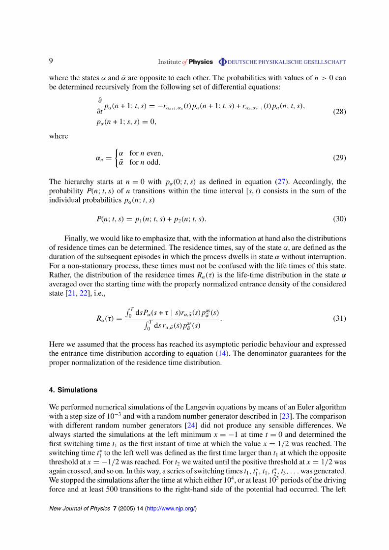
Figure 4. The variance in the number of transitions 〈δN2(T )〉 ≡ 〈δN2(T, 0)〉in one period is shown as a function of the inverse temperature. The symbolsare the same as in figure 2; the solid lines display equation (22). Note that〈δN2(T )〉 is proportional to the diffusion constant of the Rice phase. The verticalthin black lines indicate the optimal inverse temperatures as found from thesynchronization of the averaged phase (see figure 2). They coincide remarkablywell with the positions of the minima of 〈δN2(T )〉. So we find that at the optimaltemperature also the fluctuations of the number of transitions and consequentlyof the generalized Rice phase are suppressed.

of the inverse temperature. In figure 4 we compare the prediction of the two-state model, seeequation (22) with numerics. These number fluctuations exhibit a local minimum very close tothe optimal temperature where two transitions per period occur on average, see figures 2 and 4.This minimum is more pronounced for the lower driving frequency. The fluctuations of the Ricephase also assumes a minimum at this optimal temperature. This means that the phase diffusionis minimal at this temperature.

For the Fano factor F(0) we obtain an absolute minimum near the optimal temperature,see figure 5. For higher temperatures, the Fano factor may become larger than one, whereas itapproaches the Poissonian value F = 1 for low temperatures because then, transitions becomevery rare and independent from each other. Also here, theory and simulations agree indeed verywell.

Next, we consider the probabilities P(n) = P(n; T, 0) for finding N(T, 0) = n transitionsper period in the asymptotic, periodic limit. For this purpose we count the number k oftransitions within each period [nT, (n + 1)T ) and determine their relative frequency occurringin a simulation. A comparison with the prediction of the two-state model determined from thenumerical integration of equation (27) and from equation (29) is collected in figure 6 for differenttemperature values. The agreement between simulations and theory is within the expectedstatistical accuracy. For large temperatures there is a rather broad distribution of n-values arounda most probable value n∗. With decreasing temperature, the most probable value moves to smallernumbers whereby the width of the distribution shrinks. Once n∗ = 2 the probability P(2) furtherincreases at the cost of the other k values with decreasing temperature until k = 0 gains the fullweight in the limit of low temperatures.


http://www.njp.org/


0

0.25

0.5

0.75

1

1.25

1.5

Fano

-fac

tor

20 30 40 50β

Ω =10−3Ω =10−4

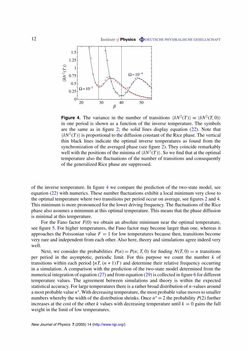
Figure 5. As a relative measure of the number and phase fluctuations, theFano factor F = F(0) from equation (26) is shown as a function of the inversetemperature. Symbols are the same as in figure 2. The minimum positions of theFano factor again nicely coincide with the optimal temperature values indicatedby the thin black lines. With decreasing frequency these minima move to lowertemperatures and become broader and deeper. For sufficiently low temperaturesthe transitions become very rare and almost Poissonian leading to the asymptoticlow temperature limit F = 1.

0

0.1

0.2

0.3

0.4

P(n

)

P(n

)

0 20 40 60 80n

β = 20, Theoryβ = 20, Simul.β = 30, Theoryβ = 30, Simul.

(a)

0

0.2

0.4

0.6

0.8

1

0 1 2 3 4 5 6n

β = 40, Theoryβ = 40, Simul.β = 55, Theoryβ = 55, Simul.

(b)

Figure 6. The probabilities P(n)=P(n; T, 0) are shown for the driving strengthA = 0.1 and the driving frequency = 10−4; for two temperatures that are higherthan the optimal one corresponding to β ≈ 40 in panel (a) and for the optimaland a lower temperature in panel (b). As one expects for a good synchronizationof the system with the driving force at the optimal temperature one finds twotransitions per period with about 90% of the total weight. For high temperaturesthe distribution becomes rather broad with a maximum at some large numberof transitions. On the contrary, for low temperatures the probability is largest atn = 0 and decreases with n. The agreement of the two-state theory resulting fromequation (30) with the simulations is remarkably good.

The degree of synchronization of the continuous bistable dynamics with the external drivingforce can be characterized by the value of the probability P(2). As a function of the inversetemperature β it has a maximum close to the corresponding optimal temperature, see figure 7.


http://www.njp.org/


0

0.2

0.4

0.6

0.8

1

P(2

)

20 30 40 50β

Ω = 10−4Ω = 10−3

Figure 7. The probability P(2) = P(n = 2; T, 0) for two transitions within oneperiod is shown as a function of the inverse temperature β. Results from thesimulations are depicted by red (×) and blue (+) crosses for two frequencies.They agree well with the respective theoretical predictions of the two-statetheory resulting from equation (30) (solid lines). The probabilities show thetypical stochastic resonance behaviour with a maximum very close to the optimaltemperature. As for the minimum of the Fano factor, this maximum is morepronounced at the lower driving frequency.

0

0.2

0.4

0.6

0.8

1

P(2

)

2 3 4 5 6−log10 Ω

Figure 8. The probability P(2) = P(n = 2; T, 0) (see equation (30)) for twotransitions within one period is shown as a function of the frequency at the inversetemperature β = 35. It also shows a resonance-like behaviour with a maximumat an optimal frequency.

For the longer driving period, the maximum is at a lower temperature and its value is higher.Figure 8 depicts P(2) as a function of the frequency at a fixed temperature. It has a maximum atsome optimal value of the frequency.

Finally, we come to the residence time distributions which can be estimated from histogramsof the simulated data. In figure 9 these histograms are compared with the results of the two-statemodel. Theory and simulations are in good agreement and show a transition from a multi-modaldistribution with peaks at odd multiples of half the period to a mono-modal distribution at zeroas one would expect. At stochastic resonance taking place at the inverse temperature β ≈ 40 thedistribution is also mono-modal with its maximum close to half the period.


http://www.njp.org/


References

[1] Gammaitoni L, Hänggi P, Jung P and Marchesoni F 1998 Rev. Mod. Phys. 70 223[2] Reimann P 2002 Phys. Rep. 361 57

Astumian R D and Hänggi P 2002 Phys. Today 55 (No. 11) 33Reimann P and Hänggi P 2002 Appl. Phys. A 75 169

[3] Rozenfeld R, Freund J A, Neiman A and Schimansky-Geier L 2001 Phys. Rev. E 64 051107Freund J A, Neiman A B and Schimansky-Geier L 2000 Europhys. Lett. 50 8Park K, Lai YC, Liu ZH and Nachman A 2004 Phys. Lett. A 326 391

[4] Callenbach L, Hänggi P, Linz S J, Freund J A and Schimansky-Geier L 2002 Phys. Rev. E 65 051110Freund J A, Schimansky-Geier L and Hänggi P 2003 Chaos 13 225

[5] Hänggi P and Thomas H 1982 Phys. Rep. 88 207[6] Jung P and Hänggi P 1990 Phys. Rev. A 41 2977

Jung P 1993 Phys. Rep. 234 175[7] Jung P and Hänggi P 1991 Phys. Rev. A 44 8032[8] Lehmann J, Reimann P and Hänggi P 2000 Phys. Rev. Lett. 84 1639

Lehmann J, Reimann P and Hänggi P 2000 Phys. Rev. E 62 6282Lehmann J, Reimann P and Hänggi P 2000 Phys. Status Solidi 237 53

[9] Schindler M, Talkner P and Hänggi P 2004 Phys. Rev. Lett. 93 048102[10] McNamara B and Wiesenfeld K 1989 Phys. Rev. A 39 4854[11] Shneidman V A, Jung P and Hänggi P 1994 Phys. Rev. Lett. 72 2682

Shneidman V A, Jung P and Hänggi P 1994 Europhys. Lett. 26 571Casado-Pascual J, Gomez-Ordonez J, Morillo M and Hänggi P 2003 Phys. Rev. Lett. 91 210601

[12] Talkner P and Łuczka J 2004 Phys. Rev. E 69 046109[13] Rice S O 1954 Mathematical analysis of random noise Selected Papers on Noise and Stochastic Processes ed

N Wax (New York: Dover) p 133[14] Talkner P 2003 Physica A 325 124[15] Gammaitoni L, Marchesoni F and Santucci S 1995 Phys. Rev. Lett. 74 1052[16] Fano U 1947 Phys. Rev. 72 26

Shuai J W and Jung P 2003 Fluct. Noise Lett. 2 L139[17] Hänggi P, Talkner P and Borkovec M 1990 Rev. Mod. Phys. 62 251[18] Talkner P 1999 New J. Phys. 1 4[19] Cox D R and Miller H D 1972 The Theory of Stochastic Processes (London: Chapman and Hall)[20] Stratonovich R L 1963 Topics in the Theory of Random Noise vol 1 (New York: Gordon and Breach)[21] Löfstedt R L and Coppersmith S N 1994 Phys. Rev. E 49 4821[22] Choi M H, Fox R F and Jung P 1998 Phys. Rev. E 57 6335[23] Matsumoto M and Nishimura T 1998 ACM Trans. Modeling Comput. Simulation 8 3[24] Lüscher M 1994 Comput. Phys. Commun. 79 100

L’Ecuyer P 1996 Math. Comput. 65 203


http://www.njp.org/

statistics of transition times, phase diffusion and

Documents