Statistics on Placenta ShapesAbhishek Bhattacharya

Department of Math, University of Arizonaabhishek@math.arizona.edu

Abstract

In this poster, I present some tools for the statistical analy-sis of placenta shapes using a random sample of placentaimages. This is part of a project carried out by me at LosAlamos National Labs over June-August 2007.

1. Introduction to Placenta shape

THe placenta is an organ developed within the uterus ofthe mother during gestation that is connected to the em-

bryo by the umbilical cord and that is discharged shortly af-ter birth. It serves as a structure through which nourishmentfor the fetus is received from, and wastes are eliminated into,the circulatory system of the mother. Figure 1 shows a pla-centa specimen.

Figure 1: Placenta 1835 image

The statistical analysis of placenta shapes based on a ran-dom sample of placentas is important in many areas. Bynoting key features of the shape, like the position of the Um-bilical Cord Insertion point (CdIns) relative to the outer andinner perimeters, the thickness of the inter perimeter region,shape of the perimeter boundaries (convexity, roundness etc)and others, one may be able to predict features of the newborn, like its gender, birth weight, presence of some dis-ease/abnormality etc.

2. Major Findings

IN my project, I compute the mean shape from a randomsample of placenta images. I find out that the mean is not

circular in shape, unlike what it seems to be (see Figure 6).

I perform a Principal Component Analysis on the tangentspace of the mean shape. I notice that perturbaion in shapealong different principal directions causes important changesin placenta shape. For example, the CdIns point moves moretowards the boundary, the mean loses its convexity etc (seeFigure 7).

I study the relation between Foetal Placental Ratio (FPR)and placenta shape by

• building a regression model explaining FPR as a functionof shape (see Table 2),

• estimating the posterior distribution of FPR given shape,using Kernel based methods.

The regression model explains about 7% of variation in FPR.The posterion distribution of FPR seems to depend a lot onhow close or far the shape is from the mean. For shapesclosest to the mean, the distribution is the most uniform,while for the most extreme shapes, it is very heterogeneous(see Table 3).

The analyses have been summarized in the subsequent sec-tions.

3. Measuring Placenta shape

TO analyze placenta shapes, we need a mathematical no-tion of shape. For that, I consider the Kendall’s planer

shape space Σk2 . I pick a set of k points on a 2D placenta

image, not all points being the same. We refer to such aset as a k-ad or a set of k landmarks. Then the shape ofa k-ad is its orbit or equivalence class under the euclideanmotions of translation, rotation and scaling. Σk

2 is the spaceof all such orbits or shapes. Thus corresponding to eachsample placenta, we get a point on Σk

2 which represents theplacenta shape. Σk

2 has the structure of the complex pro-jective space CP k−2: the space of all complex lines throughthe origin in Ck−1, which is a Riemannian manifold of dimen-sion 2k − 4. Figure 2 shows the chosen k-ad, k = 41 for aparticular placenta image.

Figure 2: All landmarks (blue) along with the selected 41landmarks (red) on Placenta 2946

The preshape of a k-ad is what remains after removing theeffects of translation and scaling. It lies on the unit sphereof dimension 2k − 3. Then the planer shape space consistsof all one dimensional orbits under rotation of the preshapes.Figure 3a shows 41 landmarks on placentas 1546 and 1528.Figure 3b shows their preshapes. Placenta 1528 preshapehas been rotated to bring it closest to the preshape of pla-centa 1546.

(a) (b)

Figure 3: (a) 41 landmarks on placentas 1546 (blue) and1528 (red), (b) Their preshapes

4. Mean on Manifolds

LEt (M,g) be a d dimensional connected complete Rie-mannian manifold, g being the Riemannian metric tensor

on M . Let ρ be a distance metrizing the topology of M . Fora given probability measure Q on M , we define the Frechetfunction of Q as

F (p) =

∫M

ρ2(p, x)Q(dx), p ∈ M. (1)

The set of all p for which F (p) is the minimum value of F onM is called the Frechet mean set of Q. If this set is a sin-gleton, say {µF}, then µF is called the Frechet mean of Q.If X1, X2, . . . , Xn are independent and identically distributed(iid) with common distribution Q, and Qn

.= 1

n

∑nj=1 δXj

is thecorresponding empirical distribution, then the Frechet meanset of Qn is called the sample Frechet mean set, denotedby CQn

. If this set is a singleton, say {µFn}, then µFn

is calledthe sample Frechet mean.

The natural choice for the distance on M is ρ = dg, thegeodesic distance under g. Then the Frechet mean (set) ofQ is called its intrinsic mean (set). If X1, X2, . . . , Xn are iidobservations from Q, then the sample Frechet mean (set) iscalled the sample intrinsic mean (set).

In case of the planer shape space Σk2 , the projection of a

preshape onto its shape is a Riemannian submersion fromthe unit sphere of dimension 2k − 3 onto Σk

2 . This makes Σk2

a complete Reimannian manifold of dimension 2k − 4. Froma result due to Kendall, W.S.(1990), if Q is a probability dis-tribution on Σk

2 with support in a geodesic ball of radius π4 ,

say B(p, π4), then it has an intrinsic mean, µI , in its support.

Also from a result due to Bhattacharya, A. and Bhattacharya,R.(2007), the sample mean from an iid sample has asymp-toticaly Normal distribution, if supp(Q) ⊂ B(µI , R), where Ris the unique solution of tan(x) = 2x, x ∈ (0, π

2).

Another notion of mean, which is much easier to computeand exists under much broader conditions is called the ex-trinsic mean on manifolds. To get that, we embed M iso-metrically into some higher dimensional euclidean space viasome map, Φ : M → Rk. We choose the distance on M as:ρ(x, y) = ‖Φ(x) − Φ(y)‖, where ‖.‖ denotes Euclidean norm(‖u‖2 =

∑ki=1 ui

2, u = (u1, u2, .., uk)′). Let Q be a probabil-ity measure on M with finite Frechet function. The Frechetmean (set) of Q with respect to the above distance, is calledthe extrinsic mean(set) of Q. If Xj (j = 1, . . . , n) are iidobservations from Q, then the sample Frechet mean(set) iscalled the extrinsic sample mean(set).

In case of M = Σk2 , we embed it into the space S(k, C) of all

k×k complex Hermitian matrices via the Veronese-Whitneyembedding Φ. S(k, C) is viewed as a (real) vector space ofdimension k2. This gives the extrinsic distance ρ on Σk

2by that induced from this embedding. Let Q be a proba-bility measure on Σk

2 , and let µ denote the mean vector ofQ

.= Q ◦ Φ−1, regarded as a probability measure on Ck2

(or,R2k2

). Then it can be shown that the extrinsic mean set of Qis the orbit under rotation of the space of unit eigenvectorsfor the largest eigen value of µ. It follows that the extrinsicmean µE, say, of Q is unique if and only if the eigenspacefor the largest eigenvalue of µ is (complex) one dimensional,and then µE is the shape of µ, µ( 6= 0) ∈ the eigenspaceof the largest eigenvalue of µ. Also it can be shown that inthat case, any measurable selection from the sample extrin-sic mean set, is a strongly consistent estimator of µE, andhas asymptotic Normal distribution with mean µE.

Using these results, we can construct one and two sampletests to draw inference on the population mean using thesample estimate.

5. Placenta Mean Shapes

GIven a sample of 1101 placenta configurations, I com-pute the extrinsic and intrinsic sample mean shapes.

These mean shapes can tell a lot about the shape distributionof the random placenta sample.

Figure 4a,b show the preshapes of the extrinsic samplemeans of 8 inner and outer landmarks respectively alongwith the corresponding sample landmarks. The samplepreshapes have been rotated and scaled so as to mini-mize their euclidean distances from the mean preshape.

−0.8 −0.6 −0.4 −0.2 0 0.2 0.4 0.6−0.8

−0.6

−0.4

−0.2

0

0.2

0.4

0.6Outer perimeter 8 landmarks for 1101 samples, along with mean shape

−0.8 −0.6 −0.4 −0.2 0 0.2 0.4 0.6−0.8

−0.6

−0.4

−0.2

0

0.2

0.4

0.6Inner perimeter 8 landmarks for 1101 sample, along with mean shape

(a) (b)

Figure 4: (a): 8 landmark outer perimeter mean shapealong with sample outer perimeters. (b): 8 landmark innerperimeter mean shape along with sample inner perimeters.

The figures suggest that both the outer and inner meanshapes are close to being circular, i.e. the 8-ad populationmean shapes should be regular octagons. To test that I per-form one sample tests, and get p-values of order smaller than10−16. The very small p-values force me to accept the alter-native hypothesis that the sample shapes come from a popu-lation whose mean shape is different from a regular octagon.Figure 5 shows the plot of the 2 means along with octagons.

−0.4 −0.3 −0.2 −0.1 0 0.1 0.2 0.3 0.4

−0.3

−0.2

−0.1

0

0.1

0.2

0.3

Circle vs Placenta outer perimeter sample mean

−0.4 −0.3 −0.2 −0.1 0 0.1 0.2 0.3 0.4

−0.3

−0.2

−0.1

0

0.1

0.2

0.3

Circle vs Placenta inner perimeter sample mean

(a) (b)

Figure 5: (a): 8 landmark outer perimeter mean shapealong with a regular octagon. (b): 8 landmark inner perimetermean shape along with a regular octagon. Red representsoctagon edges, blue are the mean shape landmarks

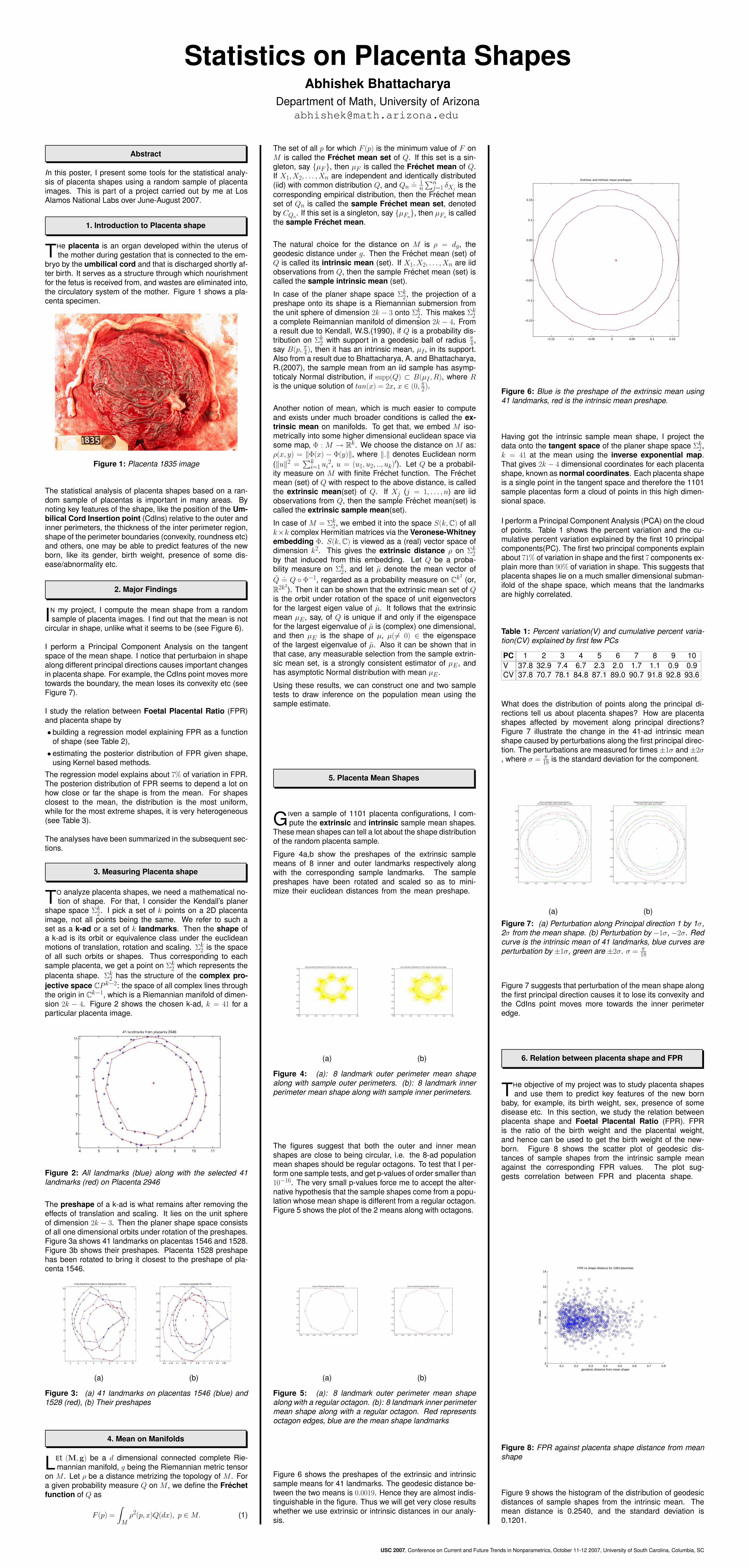
Figure 6 shows the preshapes of the extrinsic and intrinsicsample means for 41 landmarks. The geodesic distance be-tween the two means is 0.0019. Hence they are almost indis-tinguishable in the figure. Thus we will get very close resultswhether we use extrinsic or intrinsic distances in our analy-sis.

−0.15 −0.1 −0.05 0 0.05 0.1 0.15

−0.15

−0.1

−0.05

0

0.05

0.1

0.15

Extrinsic and Intrinsic mean preshapes

Figure 6: Blue is the preshape of the extrinsic mean using41 landmarks, red is the intrinsic mean preshape.

Having got the intrinsic sample mean shape, I project thedata onto the tangent space of the planer shape space Σk

2 ,k = 41 at the mean using the inverse exponential map.That gives 2k − 4 dimensional coordinates for each placentashape, known as normal coordinates. Each placenta shapeis a single point in the tangent space and therefore the 1101sample placentas form a cloud of points in this high dimen-sional space.

I perform a Principal Component Analysis (PCA) on the cloudof points. Table 1 shows the percent variation and the cu-mulative percent variation explained by the first 10 principalcomponents(PC). The first two principal components explainabout 71% of variation in shape and the first 7 components ex-plain more than 90% of variation in shape. This suggests thatplacenta shapes lie on a much smaller dimensional subman-ifold of the shape space, which means that the landmarksare highly correlated.

Table 1: Percent variation(V) and cumulative percent varia-tion(CV) explained by first few PCs

PC 1 2 3 4 5 6 7 8 9 10V 37.8 32.9 7.4 6.7 2.3 2.0 1.7 1.1 0.9 0.9CV 37.8 70.7 78.1 84.8 87.1 89.0 90.7 91.8 92.8 93.6

What does the distribution of points along the principal di-rections tell us about placenta shapes? How are placentashapes affected by movement along principal directions?Figure 7 illustrate the change in the 41-ad intrinsic meanshape caused by perturbations along the first principal direc-tion. The perturbations are measured for times ±1σ and ±2σ, where σ = π

18 is the standard deviation for the component.

−0.15 −0.1 −0.05 0 0.05 0.1 0.15

−0.2

−0.15

−0.1

−0.05

0

0.05

0.1

0.15

Positive purturbation along Principal direction 1red:mean, blue:1sigma, green:2sigma, sigma = pi/18

−0.2 −0.15 −0.1 −0.05 0 0.05 0.1 0.15

−0.15

−0.1

−0.05

0

0.05

0.1

0.15

0.2

Negative purturbation along Principal direction 1red:mean, blue:1sigma, green:2sigma.

(a) (b)

Figure 7: (a) Perturbation along Principal direction 1 by 1σ,2σ from the mean shape. (b) Perturbation by −1σ, −2σ. Redcurve is the intrinsic mean of 41 landmarks, blue curves areperturbation by ±1σ, green are ±2σ. σ = π

18

Figure 7 suggests that perturbation of the mean shape alongthe first principal direction causes it to lose its convexity andthe CdIns point moves more towards the inner perimeteredge.

6. Relation between placenta shape and FPR

THe objective of my project was to study placenta shapesand use them to predict key features of the new born

baby, for example, its birth weight, sex, presence of somedisease etc. In this section, we study the relation betweenplacenta shape and Foetal Placental Ratio (FPR). FPRis the ratio of the birth weight and the placental weight,and hence can be used to get the birth weight of the new-born. Figure 8 shows the scatter plot of geodesic dis-tances of sample shapes from the intrinsic sample meanagainst the corresponding FPR values. The plot sug-gests correlation between FPR and placenta shape.

0 0.1 0.2 0.3 0.4 0.5 0.6 0.7 0.82

4

6

8

10

12

14

geodesic distance from mean shape

FP

R v

alue

FPR vs shape distance for 1084 placentas

Figure 8: FPR against placenta shape distance from meanshape

Figure 9 shows the histogram of the distribution of geodesicdistances of sample shapes from the intrinsic mean. Themean distance is 0.2540, and the standard deviation is0.1201.

USC 2007, Conference on Current and Future Trends in Nonparametrics, October 11-12 2007, University of South Carolina, Columbia, SC

0 0.1 0.2 0.3 0.4 0.5 0.6 0.7 0.80

20

40

60

80

100

120

140

160

180Histogram of shape distances

Figure 9: Histogram of shape distance from mean shape

To see how the two are correlated, firstly I regress FPR, sayy, on the first few principal components of placenta shape,say x = (x1, x2, . . . , xt). I try a quadratic model as follows:

y = a0 +

t∑j=1

ajxj +

t∑j=1

bjx2j +

∑ ∑1≤i<j≤t

cijxixj + ε (2)

For the model (2), I estimate the coefficients, obtain 95% con-fidence intervals for the coefficients assuming a Normal dis-tribution and use the intervals to test which coefficients arenonzero at level 5%. I also compute the proportion of vari-ation in y explained by the model R2 and test whether themodel has any non zero coefficient other than a0, i.e. if thereis any interaction between y and x. Table 2 shows the re-sults of my analysis. Column 1 shows the shape componentsused in the model explaining FPR as a function of shape,column 2 lists the estimates of the coefficients in that modelthat are found to be significant at level 5%, column 3 is R2

and column 4 is the p-value for the F-test carried out to testfor interaction between y and x. If that p-value is less than5%, I accept the hypothesis that the model has some nonzero coefficient other than a0 and hence is a good model.

Table 2: Regression of FPR(y) on shape(x)

x Significant Coefficients R2 P-valuex1 a0 = 7.7, a1 = −0.64 0.0069 0.02(x1, x2) a0 = 7.75, a1 = −0.63 0.0089 0.0859(x1, x2, x3, x4) a0 = 7.7 0.0172 0.1768(x1, x2, x3, x4, ) a0 = 7.7, a5 = 2.6, 0.0338 0.1x5, x6) a6 = −2.5

(x1, x2, x3, x4, a0 = 7.7, a5 = 3.24, a6 = −3.35, 0.0668 0.004x5, x6, x7, x8) c28 = 25.7, c38 = 43.7, c47 = −25.9,

c48 = 33.5, c68 = −65.1(x5, x6) a0 = 7.7, a5 = 2.5 0.0119 0.02

Note that FPR seems to depend on the first principal com-ponent (p-value for F-test = 0.02), however adding the sec-ond component does not add new information instead justincreases the dimension thereby making the model ineffec-tive (p-value for F-test = 0.0859). The table suggests that Ishould use the model

y = a0 +

8∑j=1

ajxj +

8∑j=1

bjx2j +

∑ ∑1≤i<j≤8

cijxixj + ε (3)

This model explains about 6.7% of variation in FPR andthe p-value is 0.004 which is fairly small. It is interest-ing to note that the only non zero linear coefficients arethat of principal components 5 and 6 and there are nonon zero quadratic terms. This suggests that FPR de-pends on shape linearly through components 5 and 6. Ofcourse there are non zero interaction terms like the coeffi-cients of x2x8, x3x8, x4x7, x4x8 and x6x8. Figure 10 showsFPR as a quadratic function of principal components 5and 6. This model explains 1.19% of FPR variation.

−0.4

−0.2

0

0.2

0.4

−0.2

−0.1

0

0.1

0.22

4

6

8

10

12

14

PC − 5

Regression of FPR on shape coordinates 5, 6R2 = 0.012

PC − 6

FP

R

Figure 10: Scatter plot of FPR against x5, x6 along with bestquadratic model

Next I use nonparametric density estimation on manifolds,to estimate the posterior distribution of FPR (y) given theplacenta shape. To do that, I divide the FPR values into 5ordered classes, say, (−∞, a1], (a1, a2], (a2, a3], (a3, a4] and(a4,∞) and then estimate the probability that considering theplacenta shape alone, the placenta will fall into a particularFPR class.To get the partition points dividing the FPR classes,a1, . . . , ap, p = 4, I maximize the weighted sum of squareddistances between the means of the p + 1 groups, or equiva-lently, minimize the weighted sum of within group variations.The weights are proportional to the probability of the groups.Mathematically, I choose a = (a1, . . . , ap), p = 4 so as to max-imize

φ(a) =

p+1∑i=1

P (ai−1, ai] (E(Y |ai−1 < Y ≤ ai)− E(Y ))2 (4)

with respect to a. In (4), P denotes the FPR probabilitydistribution and Y has distribution P . There a0 = −∞ andap+1 = ∞. Given an iid sample Y1, . . . , Yn with common dis-tribution P , I get sample estimate for a, a = (a1, . . . , ap) byreplacing P in (4) by the sample empirical distribution, Pn.For this specific sample,

a1 = 5.985, a2 = 7.245, a3 = 8.354, a4 = 9.71.

Figure 11 shows the histogram of the FPR values along withthe 5 classes. Red lines denote class boundary. Note thatthere are other ways of classifying FPR values, for exam-ple that can be done based on some biological considera-tion, but for this case, I use purely statistical reasoning.

2 4 6 8 10 12 140

10

20

30

40

50

60

70

80

90

Histogram of FPR values along with the chosen 5 classesRed lines represent class boundaries

Figure 11: Histogram of FPR values classified into 5 classes

If the prior probabilities of the p + 1 classes are π =(π1, . . . , πp+1) (πj = P (aj−1, aj], j = 1, . . . , p + 1), thentheir posterior probabilities given a shape x are $(x) =($1(x), . . . , $p+1(x)) where

$j(x) =f (x|Y ∈ (aj−1, aj])πj∑p+1j=1 f (x|Y ∈ (aj−1, aj])πj

, j = 1, . . . , p + 1. (5)

Here f (x|Y ∈ (aj−1, aj]) represents the conditional shapedensity for the class Y −1(aj−1, aj]. We estimate that by theKernel density estimate,

fσj(x) =1

nj

∑j:Yj∈(aj−1,aj]

e−12

d2g(Xj,x)

σ2∫Σ41

2e−

12

d2g(y,x)

σ2 V (dy)

, j = 1, . . . , p + 1

(6)for appropriately chosen σ. Here X1, . . . , Xn is the iid shapesample and nj is the the number of shapes in the classCj = {Xi : Yi ∈ (aj−1, aj]}. Then we estimate the poste-rior probability, $j(x) by

$j(x) =fσj(x)πj∑p+1j=1 fσj(x)πj

, j = 1, . . . , p + 1. (7)

Here πj is the proportion of Yj ’s in (aj−1, aj]. For our sample,they are

π1 = 0.11, π2 = 0.30, π3 = 0.31, π4 = 0.21, π5 = 0.07.

Table 3 shows the posterior probabilities $j, j = 1, 2, . . . , 5for a few shapes when I take σ = 0.07.

Table 3: Posterior probabilities ($) for a few placentas

Placenta Id Geodesic Distance $1 $2 $3 $4 $5from mean shape

2946 0.0577 0.1015 0.2887 0.3239 0.2216 0.06422163 0.0596 0.0960 0.2983 0.3257 0.2166 0.06342919 0.0636 0.1061 0.2878 0.3202 0.2214 0.06452639 0.0637 0.0966 0.2974 0.3265 0.2139 0.06572830 0.0653 0.0869 0.3062 0.3125 0.2319 0.06253363 0.0678 0.0891 0.3020 0.3281 0.2189 0.06192561 0.0682 0.1059 0.2973 0.3259 0.2131 0.05783062 0.0746 0.0973 0.2989 0.3140 0.2116 0.07822645 0.0750 0.0966 0.3107 0.3203 0.2140 0.05842957 0.0750 0.0954 0.3036 0.3185 0.2088 0.07373303 0.2300 0.1469 0.2413 0.3114 0.1747 0.12572630 0.2306 0.1006 0.2788 0.3117 0.2288 0.08012620 0.2308 0.1268 0.4238 0.2330 0.1767 0.03972007 0.2309 0.0655 0.3128 0.2580 0.2772 0.08653396 0.2314 0.1476 0.2720 0.2931 0.1640 0.12332938 0.2318 0.4820 0.1625 0.1839 0.1035 0.06811730 0.2321 0.1166 0.3423 0.2932 0.1660 0.08182788 0.2321 0.0714 0.4759 0.1959 0.2054 0.05152648 0.2325 0.0302 0.1373 0.1312 0.6827 0.01862126 0.2326 0.1119 0.3083 0.2540 0.2491 0.07652732 0.5915 0.0001 0.9423 0.0462 0.0011 0.01031976 0.5929 0.0000 0.9993 0.0000 0.0006 0.00001762 0.6073 0.0000 1.0000 0.0000 0.0000 0.00001832 0.6105 0.0000 0.0155 0.0053 0.0019 0.97732776 0.6338 0.0148 0.9807 0.0004 0.0002 0.00401806 0.6410 0.0000 1.0000 0.0000 0.0000 0.00003244 0.6510 1.0000 0.0000 0.0000 0.0000 0.00002107 0.6525 0.0000 0.0014 0.0187 0.9798 0.00013061 0.6531 0.0000 0.0006 0.0035 0.0115 0.98441921 0.7419 0.0000 0.0000 0.0000 0.9999 0.0000

The first 10 placentas in the table are the ones with shapesclosest to the (intrinsic) mean shape. The next 10 are theones with shape distance in the middle, and the last 10 haveshapes furthest from the mean. Note how the FPR distri-bution changes for the 3 shape groups. The first group pla-centa shapes seem to have the most homogeneous condi-tional FPR distribution, while for the last 10, the distributionseems to be the least homogeneous. In the table, Placenta1806 with shape distance 0.64 belongs to class 2 , i.e. theone with FPR in (6.0, 7.2], with probability 1. That seems tobe consistent with Figure 8 because placenta 1806 has anFPR value of 7.17. However placenta 3244 with shape dis-tance 0.65 belongs to class 1, i.e. has FPR less than 6 withprobability 1 which does not seem to be consistent with Fig-ure 8, because this placenta has a FPR of 10.07 (class 5).This discrepency may be justified, if we note that our proba-bility estimates depend on the entire shape and not just onthe shape distance from the mean.

Future work

WE can get many interesting results by analyzing pla-centa shapes in more detail.

If I continue this project in future, I may carry out two sampletests to discriminate between placenta shapes of oppositesexes. Also I may carry out the regression of FPR on shapeseparately for the two sex and may get very different results.This regression can be done nonparametrically, rather thanassuming a quadratic model. In such a model, I estimate theposterior mean of FPR given placenta shape using kernelbased methods.Another important analysis will be to use placenta size andshape information to predict new born features. A measureof placenta size can be the placenta weight. Using size andshape information together, we may get much stronger mod-els explaining FPR.To get more information on shape, I may consider the shapeof 3-D configurations from the whole placentas. That requiresstatistical analysis tools on a different manifold, namely Σk

3 ,and some methodologies have been developed in recenttimes.Finally, to measure placenta shape more accurately, I mayalso include the position of the blood vessels, nerve endingsetc in the shape. These features can tell us a lot about thenew born.

USC 2007, Conference on Current and Future Trends in Nonparametrics, October 11-12 2007, University of South Carolina, Columbia, SC