statnamic lateral load testing and analysis of a drilled

Brigham Young University Brigham Young University

BYU ScholarsArchive BYU ScholarsArchive

Theses and Dissertations

2005-12-02

Statnamic Lateral Load Testing and Analysis of a Drilled Shaft in Statnamic Lateral Load Testing and Analysis of a Drilled Shaft in

Liquefied Sand Liquefied Sand

Seth I. Bowles Brigham Young University - Provo

Follow this and additional works at: https://scholarsarchive.byu.edu/etd

Part of the Civil and Environmental Engineering Commons

BYU ScholarsArchive Citation BYU ScholarsArchive Citation Bowles, Seth I., "Statnamic Lateral Load Testing and Analysis of a Drilled Shaft in Liquefied Sand" (2005). Theses and Dissertations. 723. https://scholarsarchive.byu.edu/etd/723

This Thesis is brought to you for free and open access by BYU ScholarsArchive. It has been accepted for inclusion in Theses and Dissertations by an authorized administrator of BYU ScholarsArchive. For more information, please contact [email protected], [email protected].

http://home.byu.edu/home/

http://home.byu.edu/home/

https://scholarsarchive.byu.edu/

https://scholarsarchive.byu.edu/etd

https://scholarsarchive.byu.edu/etd?utm_source=scholarsarchive.byu.edu%2Fetd%2F723&utm_medium=PDF&utm_campaign=PDFCoverPages

http://network.bepress.com/hgg/discipline/251?utm_source=scholarsarchive.byu.edu%2Fetd%2F723&utm_medium=PDF&utm_campaign=PDFCoverPages

https://scholarsarchive.byu.edu/etd/723?utm_source=scholarsarchive.byu.edu%2Fetd%2F723&utm_medium=PDF&utm_campaign=PDFCoverPages

mailto:[email protected],%[email protected]

STATMANIC LATERAL LOAD TESTING AND ANALYSIS

OF A DRILLED SHAFT IN LIQUEFIED SAND

by

Seth I. Bowles

A thesis submitted to the faculty of

Brigham Young University

in partial fulfillment of the requirements for the degree of

Master of Science

Department of Civil and Environmental Engineering

Brigham Young University

December 2005

BRIGHAM YOUNG UNIVERSITY

GRADUATE COMMITTEE APPROVAL

of a thesis submitted by

Seth I. Bowles

This thesis has been read by each member of the following graduate committee and by majority vote has been found to be satisfactory. Date Kyle M. Rollins, Chair

Date Travis M. Gerber

Date Steven E. Benzley

BRIGHAM YOUNG UNIVERSITY As chair of the candidate’s graduate committee, I have read the thesis of Seth I. Bowles in its final form and have found that (1) its format, citations, and bibliographical style are consistent and acceptable and fulfill university and department style requirements; (2) its illustrative materials including figures, tables, and charts are in place; and (3) the final manuscript is satisfactory to the graduate committee and is ready for submission to the university library. Date Kyle M. Rollins

Chair, Graduate Committee

Accepted for the Department

E. James Nelson Graduate Coordinator

Accepted for the College

Alan R. Parkinson Dean, Ira A. Fulton College of Engineering and Technology

ABSTRACT

STATMANIC LATERAL LOAD TESTING AND ANALYSIS

OF A DRILLED SHAFT IN LIQUEFIED SAND

Seth Isaac Bowles

Department of Civil and Environmental Engineering

Master of Science

Three progressively larger statnamic lateral load tests were performed on a 2.59 m

diameter drilled shaft foundation after the surrounding soil was liquefied using down-

hole explosive charges. An attempt to develop p-y curves from strain data along the pile

was made. Due to low quality and lack of strain data, p-y curves along the test shaft

could not be reliably determined. Therefore, the statnamic load tests were analyzed using

a ten degree-of-freedom model of the pile-soil system to determine the equivalent static

load-deflection curve for each test. The equivalent static load-deflection curves had

shapes very similar to that obtained from static load tests performed previously at the site.

The computed damping ratio was 30%, which is within the range of values derived from

the log decrement method.

The computer program LPILE was then used to compute the load-deflection

curves in comparison with the response from the field load tests. Analyses were

performed using a variety of p-y curve shapes proposed for liquefied sand. The best

agreement was obtained using the concave upward curve shapes proposed by Rollins et

al. (2005) with a p-multiplier of approximately 8 to account for the increased pile

diameter. P-y curves based on the undrained strength approach and the p-multiplier

approach with values of 0.1 to 0.3 did not match the measured load-deflection curve over

the full range of deflections. These approaches typically overestimated resistance at

small deflections and underestimated the resistance at large deflections indicating that the

p-y curve shapes were inappropriate. When the liquefied sand was assumed to have no

resistance, the computed deflection significantly overestimated the deflections from the

field tests.

ACKNOWLEDGMENTS

Dr. Rollins has been a wonderful professor to work with. He has been very

patient with me and the difficulties we have had with the analysis. He has always been

willing to help me when ever I needed it. He has had to spend many hours in my office

helping me try to troubleshoot the analysis. Dr. Rollins’ patience with me and explaining

difficult subjects has been invaluable.

I also need to thank Dr. Gerber for all of his help and the use of PY_BYU for

deriving the p-y curves from my strain data. Almost an entire summer was spent here in

room 192 of the Clyde Building helping me figure out how to use his program. He was

also very willing to answer any questions that I had and if he didn’t know the answer

right away he would find it.

My wonderful and supportive wife Aimee deserves an award. She has supported

me through the majority of my schooling here at BYU. She has put up with all the late

nights and boring topics I have come home talking about. Now she is also bearing the

tiring task of caring for of our new baby girl, Madison, who has her sleep schedule mixed

up. Without her love and support, I do not think I would have been able to make it

through the last bit of my schooling.

The funding for this research was provided by the National Science Foundation

(NSF) under Grant No. CMS-0085353. The support was very appreciated. The views

and recommendations expressed in this thesis are not necessarily the views of NSF.

TABLE OF CONTENTS LIST OF TABLES ......................................................................................................... xiii

LIST OF FIGURES .........................................................................................................xv

1 Introduction and Objectives .....................................................................................1

1.1 Introduction......................................................................................................1

1.2 Objective and Scope of Research ....................................................................2

1.3 Background Regarding P-Y Curves and Their Development..........................4

2 Background ................................................................................................................7

2.1 Introduction......................................................................................................7

2.2 P-Y Curve Information Prior to Full-Scale Testing.........................................8

2.3 TILT Project.....................................................................................................9

2.4 P-Y Curves Developed From TILT Testing ..................................................15

2.5 Estimating P-Multiplier Adjustments for Diameter.......................................21

2.6 Static Test on Drilled Shaft MP-1 at the Mt. Pleasant Site............................22

2.7 Brief History of the Statnamic Device (Bermingham 2000) .........................25

2.8 Statnamic Test on Drilled Shaft MP-3 at the Mt. Pleasant Site.....................26

2.9 Current Research Focus .................................................................................27

3 Site and Soil Description .........................................................................................29

3.1 Site Location and Bridge Description............................................................29

3.2 Geological Background .................................................................................32

3.3 Scope of Geotechnical Investigation .............................................................33

ixix

3.4 ..................................................33 Test Borings and Laboratory Investigations

3.5 In-Situ Testing ...............................................................................................52

3.6 Liquefaction Hazard Analysis........................................................................65

4 Test Set-Up and Pile Description............................................................................73

4.1 Introduction....................................................................................................73

4.2 Pile Description..............................................................................................73

4.3 Test Set-Up ....................................................................................................77

4.4 Above Ground Instrumentation .....................................................................79

4.5 Below Ground Instrumentation......................................................................81

4.6 Blast Layout ...................................................................................................84

5 Statnamic Lateral Load Test Results.....................................................................87

5.1 Introduction....................................................................................................87

5.2 Lateral Load Tests..........................................................................................88

5.3 Pile Motion from Acceleration Data..............................................................94

5.4 Piezometer Data ...........................................................................................114

5.5 Comparison of the Three Load Test Results................................................137

6 Analysis ...................................................................................................................149

6.1 Introduction..................................................................................................149

6.2 Calculating P-Y Curves from Strain Data ...................................................150

6.3 Empirical Evaluation ...................................................................................159

7 Conclusions.............................................................................................................183

7.1 Introduction..................................................................................................183

7.2 Blast Induced Liquefaction ..........................................................................183

7.3 Statnamic Versus Earthquake ......................................................................183

xx

7.4 Static Versus Statnamic Stiffness ................................................................184

7.5 Dynamic Versus Static Loads......................................................................184

7.6 Static Load Deflection Curves .....................................................................184

7.7 Concave Up P-Y Curves..............................................................................185

7.8 Lateral Resistance in Liquefied Sand ..........................................................185

7.9 Analysis Versus Existing Methods ..............................................................185

7.10 Recommendations........................................................................................186

References.......................................................................................................................189

Appendix A Additional Information from Testing ..............................................197

xixi

LIST OF TABLES Table 5-1 Comparison of rise time, lag time, peak acceleration, and peak velocity. ..... 139

Table 5-2 Ru values after detonation, before and after loading for load test 1............... 143



Table 6-1 Linear stiffness, natural period, and damping ratio used for each test. .......... 169

Table 6-2 Soil properties used in the analysis of Rollins et al., (2005) comparison. ..... 178

Table 6-3 Soil properties used in the analysis and comparison to the Matlock (1970)

and Wang and Reese (1998) model. ........................................................................180

Table 6-4 Soil properties used in the analysis and comparison to the Liu and Dobry

(1995) and Wilson (1998) p-multiplier models. ..................................................... 181

Table A-1 Settlement of Mt. Pleasant test site................................................................ 198

Table A-2 Compressive strengths of concrete used for the construction of MP-3......... 199

xiii

LIST OF FIGURES Figure 1-1 Derivation process used to develop p-y curves from strain

measurements (Hales, 2003)........................................................................................6

Figure 2-1 Pile head lateral load versus displacement curves for 324 mm steel

pipe piles before and after liquefaction based on Treasure Island liquefaction

testing program (Ashford and Rollins, 2000). ...........................................................11

Figure 2-2 Pile head load and excess pore pressure ratio as a function of time for

single pipe pile test at Treasure Island (written communication Kyle Rollins).........12

Figure 2-3 Measured load-displacement curves for a single pile in non-liquefied

and liquefied sand in comparison with curves computed using several values

of residual strength (written communication, Kyle Rollins). ....................................13

Figure 2-4 Expected shape of p-y curve for liquefied sand in contrast to “soft

clay” curve shape (written communication, Kyle Rollins)........................................14

Figure 2-5 Summary of calculated p-y curves for the east center pile in the 3x3

pile group during the first post-blast load series (Gerber, 2003). ..............................17

Figure 2-6 Summary of calculated p-y curves for the east center pile in the 3x3

pile group during the tenth post-blast load series (Gerber, 2003)..............................18

Figure 2-7 Post-blast p-y curves for the east center pile of the 3x3 pile group at

various depths during the first and tenth load series , where average Ru is

shown as a percent (Gerber, 2003). ...........................................................................19

xv

Figure 2-8 Post-blast p-y curves for the east center pile of the 3x3 pile group

during the first load series (Gerber, 2003). ................................................................20

Figure 2-9 Post-blast p-y curves for the east center pile of the 3x3 pile group

during the tenth load series (Gerber, 2003). ..............................................................20

Figure 2-10 Applied load versus pile head displacement curves for all three load

tests from testing on MP-1 (Hales, 2003). .................................................................23

Figure 2-11 Peak pore pressure ratio with depth immediately after the first blast

for MP-1, at the Mt. Pleasant test site........................................................................24

Figure 2-12 Peak pore pressure ratio with depth immediately after the second

blast for MP-1, at the Mt. Pleasant test site. ..............................................................24

Figure 3-1 Aerial photograph of Cooper River bridges and test site. (taken from a

presentation by the SCDOT and S&ME to the CE Club)..........................................30

Figure 3-2 Site map showing approximate locations of SPT and CPT borings (a)

relative to the existing bridge approach ramps and (b) relative to the test site

(Brown, 2000). ...........................................................................................................31

Figure 3-3 Artist's rendering of future Ravenel Bridge (Bridgepros, 2005).....................32

Figure 3-4 Boring log for test hole DS-1 (Hales 2003). ....................................................37

Figure 3-5 Boring log for test hole MPS-11 (Hales 2003). ...............................................42

Figure 3-6 Boring log for test hole LB-28 (Hales 2003). ..................................................44

Figure 3-7 Idealized soil profile for the Mt. Pleasant test site (Modified from

Camp et al., 2000a). ...................................................................................................49

Figure 3-8 Atterberg limits tests at various depths within the Cooper River Marl

relative to the plasticity chart (Camp et al., 2000b)...................................................50

xvi

Figure 3-9 Natural moisture content versus elevation in the Cooper River Marl

(Camp et al., 2000b)...................................................................................................50

Figure 3-10 Fines content versus elevation in the Cooper River Marl (Camp et al.,

2000b). .......................................................................................................................51

Figure 3-11 Undrained shear strength versus elevation from UU and CU triaxial

shear test on undisturbed samples of the Cooper River Marl (Camp et al.,

2000b). .......................................................................................................................51

Figure 3-12 Results of drained triaxial shear strength tests on Cooper River Marl

plotted in a p-q diagram (Camp et al., 2000b). ..........................................................52

Figure 3-13 Normalized SPT clean sand penetration resistance versus depth for

three test holes near the test site.................................................................................54

Figure 3-14 Interpreted relative density versus depth based on SPT penetration

resistance for three holes close to the test site. ..........................................................55

Figure 3-15 Results from CPT sounding LTB-1 including normalized cone

resistance, friction ratio, and pore pressure along with interpreted relative

density and soil profile...............................................................................................57

Figure 3-16 Results from CPT sounding MPS-7 including normalized cone

resistance, friction ratio, and pore pressure along with interpreted relative


Figure 3-17 Results from CPT sounding GT-1 including normalized cone

resistance friction ratio, and pore pressure along with interpreted relative


xvii

Figure 3-18 Interpreted Relative density and friction angle versus depth for sand

layers in the soil profile based on three CPT soundings............................................62

Figure 3-19 Interpreted Undrained shear strength versus depth for clay layers in

the soil profile based on three CPT soundings...........................................................63

Figure 3-20 Profiles of Vs and Vs1 versus depth based on down SCPT sounding

and a down-hole shear wave velocity test conducted by Redpath Geophysics. ........65

Figure 3-21 Photograph of a brick house wrecked by the Charleston earthquake of

August 31, 1886 (USGS, 2005). ...............................................................................68

Figure 3-22 Photograph of a sand boil due to liquefaction during the 1886

Charleston, South Carolina Earthquake (FHWA, 2005). ..........................................69

Figure 3-23 Profiles showing cone tip resistance, SBT index, and factor of safety

against liquefaction versus depth for GT-1 due to M7.3 earthquake

producing 0.77 g peak acceleration associated with a 2% probability of

exceedance in 50 years. (Hales, 2003)......................................................................70

Figure 3-24 Profiles showing cone tip resistance, SBT index, and factor of safety

against liquefaction versus depth for GT-1 due to M6.4 earthquake

producing 0.16 g peak acceleration associated with a 10% probability of

exceedance in 50 years. (Hales 2003).......................................................................71

Figure 4-1 Contractor used a track-mounted SoilMec for drilling (photograph

from a presentation by the SCDOT and S&ME to the CE Club). .............................74

Figure 4-2 Photograph of worker assembling reinforcement cage at the Mount

Pleasant site (photograph from a presentation by the SCDOT and S&ME to

the CE Club). .............................................................................................................75

xviii

Figure 4-3 Drilled shaft dimensions, strain gauges, and accelerometers...........................76

Figure 4-5 Drilled shaft and corresponding soil profile.....................................................77

Figure 4-6 Schematic of statnamic load test at the Mt. Pleasant site (drawing

modified from the Ravenel Bridge Project Load Test Plans). ...................................78

Figure 4-7 Schematic of the statnamic loading device with accelerometers and

LVDTs at the Mount Pleasant site (Figure provided by AFT Inc. load report

for MP-3). ..................................................................................................................80

Figure 4-8 Reinforcement cage after installation of strain gages and inclinometers

(photograph from a presentation by the SCDOT and S&ME to the CE Club)..........82

Figure 4-9 Plan view of the piezometers and charges (Brown, 2000)...............................83

Figure 4-10 Elevation view showing a profile of piezometers and down-hole

charges relative to the test shaft. ................................................................................84

Figure 5-1 Pile head deflection time history for the first lateral load test on test

pile MP-3. ..................................................................................................................89

Figure 5-2 Load time history for the first lateral load test on test pile MP-3. ...................89

Figure 5-3 Load versus deflection curve for load test 1 on test pile MP-3........................90

Figure 5-4 Pile head deflection time history for the second lateral load test on test

pile MP-3 ...................................................................................................................91

Figure 5-5 Load time history for the second lateral load test on test pile MP-3................91

Figure 5-6 Load versus Deflection for load test 2. ............................................................92

Figure 5-7 Pile head deflection time history for the third lateral load test on test

pile MP-3. ..................................................................................................................93

Figure 5-8 Load time history for the third lateral load test on test pile MP-3. ..................93

xix

Figure 5-9 Load versus Deflection curve for load test 3. ..................................................94

Figure 5-10 Acceleration, velocity, and deflection graphs from test 1

accelerometers............................................................................................................97

Figure 5-11 (Continued) Acceleration, velocity, and deflection graphs from test 1

accelerometers............................................................................................................98

Figure 5-12 (Continued) Acceleration, velocity, and deflection graphs from load

test 1 accelerometers. .................................................................................................99

Figure 5-13 (Continued) Acceleration, velocity, and deflection graphs from load

test 1 accelerometers. ...............................................................................................100

Figure 5-14 Acceleration versus depth plots plot at several times for load test 1. ..........100

Figure 5-15 Velocity versus depth plots derived from accelerations at several

times for load test 1..................................................................................................101

Figure 5-16 Deflection versus depth plots derived from accelerations at several

times for load test 1 along with measured deflections from LVDTs above

ground. .....................................................................................................................101

Figure 5-17 Acceleration, velocity, and deflection graphs from load test 2

accelerometers..........................................................................................................103

Figure 5-18 Acceleration versus Depth time step plot from load test 2. .........................106

Figure 5-19 Velocity versus Depth time step plot from load test 2. ................................107

Figure 5-20 Deflection versus Depth time step plot from load test 2..............................107

Figure 5-21 Acceleration, velocity, and deflection graphs from load test 3

accelerometers..........................................................................................................109

Figure 5-22 Acceleration versus Depth time step plot from load test 3. .........................112

xx

Figure 5-23 Velocity versus Depth time step plot from load test 3. ................................113

Figure 5-24 Deflection versus Depth time step plot from load test 3..............................113

Figure 5-25 Ru time histories from the first blast for (a) B5, (b) B6, and (c) B3. ...........118

Figure 5-26 Ru time histories from the first blast for (a) B7, (b) B2, and (c) B8. ...........119

Figure 5-27 Ru time histories from the first blast for (a) B1, (b) B11, and (c) B10. .......120

Figure 5-28 Ru time histories from the first blast for (a) B12, (b) B13, and (c)

B15...........................................................................................................................121

Figure 5-29 Peak Ru versus depth plots for the first load test immediately after the

charges were detonated. ...........................................................................................122

Figure 5-30 Peak Ru versus depth for the first load test just after the statnamic

device was fired. ......................................................................................................123

Figure 5-31 Ru time histories from the second blast for (a) B5, (b) B6, and (c) B3........125

Figure 5-32 Ru time histories from the second blast for (a) B7, (b) B2, and (c) B8........126

Figure 5-33 Ru time histories from the second blast for (a) B1, (b) B11, and (c)

B10...........................................................................................................................127

Figure 5-34 Ru time histories from the second blast for (a) B12, (b) B13, and (c)

B15...........................................................................................................................128

Figure 5-35 Peak Ru versus depth plots for the second load test immediately after

the charges were detonated. .....................................................................................129

Figure 5-36 Peak Ru versus depth plots for the second load test immediately after

the statnamic device was fired. ................................................................................130

Figure 5-37 Ru time histories from the third blast for (a) B5, (b) B6, and (c) B3. ..........132

Figure 5-38 Ru time histories from the third blast for (a) B7, (b) B2, and (c) B8. ..........133

xxi

Figure 5-39 Ru time histories from the third blast for (a) B1, (b) B11, and (c) B10. ......134

Figure 5-40 Ru time histories from the third blast for (a) B12, (b) B13, and (c)

B15...........................................................................................................................135

Figure 5-41 Peak Ru versus depth plots for the third load test immediately after

the charges were detonated. .....................................................................................136

Figure 5-42 Peak Ru versus depth plots for the third load test immediately after

the statnamic device was fired. ................................................................................137

Figure 5-43 Comparison of the three applied pile head load versus deflection

curves. ......................................................................................................................139

Figure 5-44 Maximum positive and negative acceleration, velocity, and deflection

for all three tests.......................................................................................................142

Figure 5-45 Comparison of the piezometer readings for the three tests. .........................143

Figure 5-46 Excess pore pressure ratio contours (in percent) for the soil profile

mass immediately after the detonation of the charges for test 1..............................145

Figure 5-47 Excess pore pressure ratio contours ( in percent) for the soil mass

immediately after the statnamic loading for test 1...................................................145

Figure 5-48 Excess pore pressure ratio contours (in percent) for the soil mass

immediately after the detonation of the charges for test 2......................................146




immediately after the detonation of the charges for test 3.......................................147

xxii



Figure 6-1 Time step curvatures calculated from strain gauges for test 1 of MP-3.........152



Figure 6-4 Model used to calculate the inertial force (relative size of the masses

provides an approximate indication of mass distribution).......................................162

Figure 6-5 Deflection profile for load test 3 used to find the active length.....................163

Figure 6-6 Comparison of load-deflection curves for test 1. ...........................................168

Figure 6-7 Comparison of load-deflection curves for test 2. ...........................................168

Figure 6-8 Comparison of load-deflection curves for test 3 ............................................169

Figure 6-9 Plots of the measured statnamic force time history, computed inertia,

damping and spring force time histories for test 1...................................................169





Figure 6-12 Comparison of the static equivalent load-deflection curves for all

three tests. ................................................................................................................171

Figure 6-13 Average pore water pressures for the first blast, first cycle and the

second blast, first cycle compared to the average pore pressures of all three

load tests of MP-3. ...................................................................................................173

xxiii

Figure 6-14 Comparison of the load deflection curve of the first blast of MP-1 and

the static equivalent load deflection curve of MP-3. ...............................................174

Figure 6-15 Comparison of the load deflection curve of the second blast of MP-1

and the static equivalent load deflection curve of MP-3..........................................174

Figure 6-16 Relationship between residual strength and corrected SPT resistance

(Seed and Harder, 1990). .........................................................................................179

Figure 6-17 Comparison of the use of soft clay p-y curve for liquefied sand versus

the calculated static equivalent for test 2 of MP-3...................................................180

Figure 6-18 Comparison of the method used by Liu and Dobry (1995) and Wilson

(1998) compared to the calculated equivalent static stiffness of MP-3. ..................182

Figure A-1 MP-3 drilled shaft alignment measured by Trevi Icos Corporation..............197

Figure A-2 Graph showing the recorded settlement for the Mt. Pleasant test site

while testing MP-3..................................................................................................198

xxiv

1 Introduction and Objectives

1.1 Introduction

The lateral load capacity of deep foundations is critically important in the design

of bridges, buildings and other structures in seismically active regions. Although fairly

reliable methods have been developed for predicting the lateral resistance of piles in non-

liquefied soils, there is little information to guide engineers in the design of piles that are

surrounded by liquefiable soils. Without an accurate assessment of the resistance-

displacement relationship for piles in liquefied soils, it becomes impossible to determine

whether additional piles may be necessary for a foundation in liquefied sand or whether

soil improvement must be undertaken to inhibit the development of liquefaction.

Improper assessments can lead to seismically unsafe structures or unnecessary expense.

These issues become even more important as the engineering profession attempts to

move to performance-based design codes where estimates of displacements are required.

While ongoing centrifuge studies using small-scale models can provide valuable insights,

full-scale tests are necessary to verify/calibrate these models and provide ground truth

information.

1

1.2 Objective and Scope of Research

The world’s first full-scale lateral pile load tests, utilizing controlled blasting to

achieve liquefaction within the surrounding soil, were performed during 1998 and 1999

at Treasure Island in San Francisco Bay. This thesis describes the second set of full-scale

laterally loaded tests involving blast-induced liquefaction which were conducted near

Charleston, South Carolina in 2000.

The testing in Charleston provides a valuable opportunity to expand and

supplement the data and results that were obtained from Treasure Island. For example,

the diameters of the pile foundations at the Treasure Island test site were typically about

one eighth the diameter of the shaft foundations used in Charleston. This difference

allows for an evaluation of the effect of a much wider and stiffer pile on the p-y cures. In

addition, the liquefied thickness at Treasure Island was on the order of 6 to 8 m while that

at the Charleston site was about 12 m. This deeper liquefied zone makes it possible to

evaluate the effect of greater initial effective stress (or greater depth) on the p-y curves.

Finally, in contrast to the Treasure Island tests, which were conducted statically using

only hydraulic actuators, the tests in Charleston were conducted both statically and

dynamically using a statnamic rocket sled to apply load in about 0.2 seconds. These test

results make it possible to evaluate the influence of rate of loading and damping on the

measured lateral resistance and p-y curves. The analysis of the static testing at

Charleston was the subject of a thesis by Hales (2003), while this thesis will focus on the

analysis of the dynamic testing.

2

The overall objective of this study is to better understand the resistance the large

diameter deep foundations provide in liquefied soil through full-scale testing.

Specifically, the objectives of this study are to:

1. Develop p-y curves for the liquefied soil to determine whether they correlate

with the concave-up shaped curves developed by Wilson (1998) through

centrifuge testing and those resulting from analysis of the Treasure Island Tests

(Ashford and Rollins, 2002; Rollins et al., 2005).

2. Evaluate the influence of increasing depth, initial effective stress and excess

pore pressure ratio on p-y curves in liquefied sand.

3. Quantify the effect of a stiffer, larger diameter pile on the generated p-y curves

when compared with those derived by Rollins et al., (2005) for smaller diameter

piles.

4. Determine the effect of dynamic loading on the lateral resistance of a pile in

liquefied sand relative to the static resistance.

The South Carolina Department of Transportation (SCDOT) provided funding for

the conventional axial and lateral load tests as well as the liquefaction load tests. The

tests were performed on the Mt. Pleasant side of the Cooper River near the location

where the Ravenel Bridge was proposed to be built. Modern Continental South, Inc.

served as the general contractor for the testing project and supervised the Mt. Pleasant

site testing. The test results were originally intended to aid in the design of the bridge,

but Dr. Rollins of Brigham Young University was able to procure a grant from the

National Science Foundation to allow for a more detailed analysis of the data. Therefore,

this study benefits from $250,000 already spent by the SCDOT for the foundation testing

3

and instrumentation. Although there were many tests performed at the Mt. Pleasant site,

this thesis will only focus on the analysis and interpretation of the data collected from the

statnamic lateral load test in liquefied soil performed on the foundation labeled MP-3.

1.3 Background Regarding P-Y Curves and Their Development

The lateral resistance of a deep foundation is a function of both the structural

stiffness of the foundation itself and the resistance of the surrounding soil. Therefore,

engineering analysis of soil-structure interaction problems such as this requires accurate

assessments of the non-linear behavior of both the surrounding soil and the foundation.

The lateral resistance which the soil provides is a non-linear function of the lateral

deflection of the foundation. A graphical representation of the relationship between

resistance and deflection is portrayed graphically as a p-y curve. The p-y curve is plotted

with the horizontal deflection (y) on the abscissa or the x-axis and the soil resistance

expressed as a force per length of foundation (p) on the ordinate or the y-axis.

Soil type plays a significant role in the variation of the stiffness and shape of p-y

curves. Other important factors include pile diameter, embedment depth, and various soil

properties such as strength and unit weight. In general, the lateral resistance (p) tends to

increase with increasing diameter of pile and with increasing depth below the ground

surface. A number of investigators have developed equations for p-y curves in stiff clay,

soft clay and non-liquefied sand; however, considerable uncertainty exists regarding

appropriate p-y curves for liquefied sand and how these curves might be affected by

initial vertical stress and pile diameter. Insight into factors to account for these effects

can be obtained from full-scale testing.

4

Because it is impossible to directly measure the deflection and soil pressure with

depth, an indirect method has been used along with basic beam theory. Strain gauges

along the length of the pile allow for the curvature of the pile to be evaluated. From this

curvature the pile deflection and soil pressure can be calculated. The first assumption

needed to derive the deflections is that the pile acts like an idealized Timoshenko beam.

This means that deflections are a result of bending only, and deflections due to shear are

neglected. These assumptions are only valid in long slender beams. Most piles fit the

criteria of being a slender beam. Deflection is calculated from double integration of the

curvatures with respect to the pile length. To be able to do this integration, a cantilever

support condition is often assumed, where the deflection and curvature at the bottom end

of the pile is assumed to be zero. Once again, this assumption is generally acceptable for

deep foundations.

Moment can be derived from curvature by multiplying the curvature by the

appropriate bending stiffness (or EI). From the moment, the pressure can be derived

through double differentiating moment with respect to distance along the pile. Since

pressure derived from moment is a material dependent calculation, the non-linear EI for a

concrete pile must be accurately estimated to reliably compute pressure. This

relationship will be discussed further in Chapter 6. Figure 1-1 gives a step by step

process used to develop p-y curves from strain data.

5

Figure 1-1 Derivation process used to develop p-y curves from strain measurements (Hales, 2003).

6

2 Background

2.1 Introduction

Centrifuge model testing has been the primary method for evaluating the lateral

resistance of piles in liquefied soils. Although model testing is important because it

facilitates parametric studies, it can’t represent a full-scale test completely. Cost is the

main reason why scale model testing is used and will continue to be used. Full-scale tests

have been performed which allow us to compare the model test results with actual

performance data representing a few parameter. Since full-scale testing provides the

actual response of a foundation we can substantiate the results of model testing and then

apply the combined results of both model and full-scale tests to foundation design with

confidence.

In Section 2.2, information regarding p-y curves for liquefied soils prior to full

scale testing will be presented. Since the Treasure Island Liquefaction Test (TILT)

program was the first full-scale test of its kind to be performed, a detailed review of this

test will be given. Section 2.3 will review the preliminary test results from the TILT

project. Section 3.2.4 will review the p-y curves developed by Gerber (2003) from the

TILT project data and subsequently reported by Rollins et al, (2005). Section 2.5 will

discuss p-y curves as a function of pile diameter based on the TILT test results. Section

2.6 will introduce the lateral load testing program conducted at the M. Pleasant site near

7

Charleston, South Carolina, with a focus on the analysis of liquefied soil response under

static loading. Section 2.7 will provide a brief history of statnamic testing. Section 2.8

will focus on the testing of liquefied soils at the Mt. Pleasant site using the statnamic

device and the subsequent analysis of the soil response made by Brown (2000) of ATF.

Finally Section 2.9 will address the particular focus of this thesis.

2.2 P-Y Curve Information Prior to Full-Scale Testing

Existing information regarding p-y curves for liquefied sand is still indefinite

even though research in this field has been going on for some time. In 1995, a greater

interest in this topic was initiated, and since then much more research has been conducted

to solidify the opinions and research results to converge on a design methodology.

Wang and Reese (1998) proposed that the resistance in liquefied sand can be

explained by the p-y curve for soft-clay (e.g. Matlock, 1970) if the ultimate strength is set

equal to the undrained residual shear strength of sand. Wang and Reese use the work of

Seed and Harder (1990) to suggest the undrained residual shear strength of sand can be

estimated using correlations with apparent relative density.

Through centrifuge model testing in medium dense sand with a relative density of

60%, Liu and Dobry (1995) found that the ultimate strength of fully liquefied sand was

one tenth its non-liquefied strength. So using this multiplier of 0.1 with p-y curves back

calculated from tests in non-liquefied sand, a reasonable match was made with measured

bending moments from a model pile. After more centrifuge tests in sand with a relative

density of about 40%, Abdoun (1997) agreed with the 0.1 multiplier from Liu and Dobry.

In other research efforts, Tokimatsu (1999) found that a p-multiplier ranging from 0.05 to

8

0.2 gave good representations of the observed field performance of piles subject to lateral

spreading.

In other centrifuge studies conducted at U.C. Davis Wilson (1998) derived p-y

curves for liquefied sand using a set of ground shaking time histories. Wilson compared

his p-y curves to API (1993) sand and found the p-multiplier to be 0.1 to 0.2 for loose

sand (~35% relative density) during peak loading cycles while the sand was liquefied.

He also found that for medium dense sand (~55% relative density) that the p-multiplier

was around 0.25 to 0.35. At different times in the loading time history p-multipliers of

more that 1 existed and later on in the loading time history p-multipliers ranged from 0.10

to 0.35 after the soil had lost significant amount of resistance due to cyclic loading.

Goh (2001) is another person that used centrifuge testing to produce p-y curves.

He used data from the results of Abdoun (1997) and analytical studies to try and develop

a dimensionless p-y curve for liquefied sand. His resulting p-y curve shape was different

from all the other researchers that used the p-multiplier approach.

From the review of past research on p-y curves for liquefied soil, there is a need

for further research like the TILT project and the current project in Charleston. Full-scale

testing will hopefully shed a little more light on the soil resistance in liquefied soil.

2.3 TILT Project

To improve our understanding of the lateral load behavior of deep foundations in

liquefied soil, a series of lateral load tests were recently conducted on full-scale piles, pile

groups, and drilled shaft foundations (Ashford and Rollins, 2000; Ashford and Rollins,

2002). The testing was conducted at the National Geotechnical Test Site on Treasure

9

Island in San Francisco Bay and is known as the Treasure Island Liquefaction Test, or

TILT, program. Tests were performed after a surface layer of soil was liquefied using

controlled blasting techniques. These tests were very successful and demonstrated that

controlled blasting can induce liquefaction in a well-defined volume of soil in the field

for full-scale experimentation. Excess pore pressure ratios (Ru) of 90 to 100% were

generated within a depth range of 1 to at least 6 m and over a 13 m x 19 m surface area.

Ru values greater than 80% were typically maintained for 6 minutes (Rollins et al. 2000).

The TILT project represents the first full-scale tests ever performed on deep foundations

in liquefied soils.

A typical plot of load versus displacement for a lateral load test on a single pile at

Treasure Island is shown in Figure 2-1. The test was performed using displacement-

control procedures and forces applied to the pile head were measured with load cells.

Initially, single cycles with maximum displacements of 75, 150, and 225 mm were

applied, and then nine additional cycles were applied with a maximum displacement of

225 mm. As cycling continued, the load-displacement curves rapidly degraded to an S-

shaped curve that was relatively consistent. A comparison with the load-displacement

curve prior to liquefaction indicates that the reduction in strength following liquefaction

is substantial. For the S-shape curve, very little resistance was developed initially, but

after a displacement of about 75 mm there was a rapid increase in resistance with

continued displacement. This increase in the pile-soil system stiffness appears to be tied

to the development of reduced pore water pressures due to dilation of the sand following

continued displacement. A time history of the measured excess pore pressure ratio (Ru)

is shown in Figure 2-2 along with a time history of measured load on the pile. At the

10

beginning of each cycle Ru is near 100%, indicating complete liquefaction. As

displacement increases in each cycle, Ru drops substantially and this drop in pore

pressure produces a corresponding increase in lateral resistance.

-100

-50

0

50

100

150

200

250

-50 0 50 100 150 200 250

Displacement (mm)

Load

(kN

)

Non-LiquefiedLiquefied

Figure 2-1 Pile head lateral load versus displacement curves for 324 mm steel pipe piles before and after liquefaction based on Treasure Island liquefaction testing program (Ashford and Rollins, 2000).

11

-40

-20

0

20

40

60

80

100

0 120 240 360 480 600

Time (sec)

Ru

(%)

-50

0

50

100

150

200

0 120 240 360 480 600

Time (sec)

Load

(kN

)

Figure 2-2 Pile head load and excess pore pressure ratio as a function of time for single pipe pile test at Treasure Island (written communication Kyle Rollins).

Preliminary lateral load analyses were performed to provide a rough assessment

of existing methods for developing p-y curves in liquefied sand. Figure 2-3 shows the

measured load-displacement relationships for one cycle before and after liquefaction.

Load-displacement curves computed using the computer program LPILE (2004) and are

12

also shown in Figure 2-3 for three different cases. IN two of the LPILE analyses, the

liquefied sand was assumed to have a “soft-clay” p-y curve with a residual undrained

strength equal to the lower-bound and average values obtained from correlation with the

(N1)60 value for the sand using the relationship of Seed and Harder (1990). At lower

displacement levels, the computed resistance was significantly higher than the measured

resistance, but at higher displacements, the measured resistance was within the range of

computed values.

-100

-50

0

50

100

150

200

-50 0 50 100 150 200 250 300 350

Displacement (mm)

Load

(kN

)

Non-LiquefiedLiquefiedLPILE-Avg ResidualLPILE-Low ResidualLPILE-No Residual

Figure 2-3 Measured load-displacement curves for a single pile in non-liquefied and liquefied sand in comparison with curves computed using several values of residual strength (written communication, Kyle Rollins).

In the third LPILE analysis, the liquefied sand was assumed to have no resistance

at all. In this case, the computed load-displacement curve was very close to the measured

curve at low displacements suggesting that there is little to no soil resistance acting.

13

However, at displacements greater than about 75 mm, the measured resistance rapidly

increased beyond the computed value. These preliminary results suggested that the p-y

curve for liquefied sand would have a shape that is concave upward as shown in Figure

2-4 which is in stark contrast with the “soft clay” curve shape that is typically assumed.

However a concave down p-y curve shape similar to the soft clay curve was reported by

Wilson (1998) in his interpretation of centrifuge tests.

Horizontal Displacement, y

Hor

izon

tal R

esis

tanc

e/Le

ngth

, P

Liquefied Sand Based on Soft Clay Curve

Liquefied SandSuggested by Treasure Island Testing

Figure 2-4 Expected shape of p-y curve for liquefied sand in contrast to “soft clay” curve shape (written communication, Kyle Rollins).

14

2.4 P-Y Curves Developed From TILT Testing

Results from the TILT project p-y curves are published in Gerber’s dissertation,

P-Y Curves for Liquefied Sand Subject to Cyclic Loading Based on Full-Scale Testing of

Deep Foundations (2003). A portion of the curves he developed will be subsequently

presented. The results from the TILT project confirm the assumption that the p-y curves

would present themselves as concave-up, reflective of the load-displacement curve for

the pile head.

Gerber analyzed a 3x3 group of 324 mm diameter steel pipe piles along with a

single 324mm diameter steel pipe pile. In Gerber’s dissertation, he presented p-y curves

for five of the nine piles tested and the single pipe pile. After review of the results, the

east pile in the center row appeared to be the most reliable and representative. Figure 2-5

shows the plots generated of the p-y relationship from the first load series of the tests for

the first 10 strain gage depths or stations, and Figure 2-6 shows the p-y relationship from

the tenth load series for the first 10 stations. Figure 2-7 shows comparisons of simplified,

lower bound p-y curves from the first and tenth load series for the first 7 stations. Figure

2-8 and Figure 2-9 show the same p-y curves as displayed in Figure 2-7, but with the

various curves for the same series on the same plot.

From the TILT test, Gerber’s analytical results, and study of p-y plots like the

ones shown, the following conclusions are reached:

1. P-y curves for liquefied soils are characterized by a concave-up shape where the

stiffness of the curve increases with displacement (as seen in Figure 2-7 through

Figure 2-9).

15

2. The concave-up shape seems to result primarily from dilation of the soil due to

shearing as the pile is displaced. Gapping effects, however, likely also

contribute to the observed shape of the p-y curves.

3. The stiffness of p-y curves for liquefied soils increase with increasing depth (as

seen in Figure 2-8 and Figure 2-9) and decreasing excess pore water pressure

(as seen in Figure 2-7). The p-y curves appear to transition from a concave-up

to a concave-down shape with decreasing excess pore water pressures.

4. As already mentioned in section 2.3, the concave-up shape of the p-y curves

derived for liquefied sand is starkly different from the shape given from a

residual undrained shear strength design approach. The same difference exists

with a p-multiplier design approach (Gerber 2003). Using LPILE, it was

confirmed that the derived p-y curves yield better matches with the measured

pile head deflections and moment curves over a large range of applied loads

than the p-y curves using these two design approaches.

16

Avg. Ru = 94% Avg. Ru = 76%

Avg. Ru = 85% Avg. Ru = 98%

Avg. Ru = 100% Avg. Ru = 100%

Avg. Ru = 98%

20 cm

100 kN/m

J

20 cm

100 kN/m

I

20 cm

100 kN/m

H

20 cm

100 kN/m

G

20 cm

100 kN/m

F

20 cm

100 kN/m

E

20 cm

100 kN/m

D

20 cm

100 kN/m

C

20 cm

100 kN/m

B

20 cm

100 kN/m

A

DepthBelowGroundSurface(meters)

0.00 A

0.76 B

1.52 C

2.29 D

3.05 E

3.81 F

4.57 G

5.33 H

6.10 I

6.86 J

7.62

8.38

9.14

10.67

LoadPoint

Figure 2-5 Summary of calculated p-y curves for the east center pile in the 3x3 pile group during the first post-blast load series (Gerber, 2003).

17

Avg. Ru = 63% Avg. Ru = 56%

Avg. Ru = 70% Avg. Ru = 77%

Avg. Ru = 65% Avg. Ru = 66%

Avg. Ru = 51%

20 cm

100 kN/m

J

20 cm

100 kN/m

I

20 cm

100 kN/m

H

20 cm

100 kN/m

G

20 cm

100 kN/m

F

20 cm

100 kN/m

E

20 cm

100 kN/m

D

20 cm

100 kN/m

C

20 cm

100 kN/m

B

20 cm

100 kN/m

A


0.00 A

0.76 B

1.52 C

2.29 D

3.05 E

3.81 F

4.57 G

5.33 H

6.10 I

6.86 J

7.62

8.38

9.14

10.67

LoadPoint

Figure 2-6 Summary of calculated p-y curves for the east center pile in the 3x3 pile group during the tenth post-blast load series (Gerber, 2003).

18

5 cm 10 cm 15 cm

25 kN/m

75 kN/m

51

98

G

5 cm 10 cm 15 cm

25 kN/m

75 kN/m

66

100

F5 cm 10 cm 15 cm

25 kN/m

75 kN/m

65

100

E

5 cm 10 cm 15 cm

25 kN/m

75 kN/m

77

98

D5 cm 10 cm 15 cm

25 kN/m

75 kN/m

70

85

C

5 cm 10 cm 15 cm

25 kN/m

75 kN/m

56

76

B5 cm 10 cm 15 cm

25 kN/m

75 kN/m

63 94

A


0.00 A

0.76 B

1.52 C

2.29 D

3.05 E

3.81 F

4.57 G

5.33

6.10

6.86

7.62

8.38

9.14

10.67

LoadPoint

Figure 2-7 Post-blast p-y curves for the east center pile of the 3x3 pile group at various depths during the first and tenth load series , where average Ru is shown as a percent (Gerber, 2003).

19

0 5 10 15Deflection (cm)

0

25

50

75So

il R

esis

tanc

e (k

N/m

)

A

DEFG

Curve Depth Avg. Ru A 0.00 m 94% D 2.29 m 98% E 3.05 m 100% F 3.81 m 100% G 4.57 m 98%(B & C omitted, Avg. Ru < 90%)

Figure 2-8 Post-blast p-y curves for the east center pile of the 3x3 pile group during the first load series (Gerber, 2003).

0 5 10 15Deflection (cm)

0

25

50

75

Soil

Res

ista

nce

(kN

/m)

A

BCDEF

G

Curve Depth Avg. Ru A 0.00 m 63% B 0.76 m 56% C 1.52 m 70% D 2.29 m 77% E 3.05 m 65% F 3.81 m 66% G 4.57 m 51%

Figure 2-9 Post-blast p-y curves for the east center pile of the 3x3 pile group during the tenth load series (Gerber, 2003).

20

2.5 Estimating P-Multiplier Adjustments for Diameter

As part of the TILT Project Weaver (2001) developed p-y curves for drilled

shafts. The subsurface and loading conditions for the shafts and piles analyzed by

Weaver and Gerber (200), respectively, are very similar. Because of these similarities

coupled with the apparent lack of group effects in the pile group when the soil was fully

liquefied, it is reasonable to assume the main difference between the p-y curves of

Weaver and Gerber was the diameter of the foundation.

Even though Weaver used different analysis procedures to derive his p-y curves

when six p-y curves from the 324 mm steel pipe pile, were scaled using a 5.56 multiplier

a good match was made with the 0.9 m drilled shaft. This suggests that a multiplier to

account for differing foundation diameter can be applied to a general p-y curve equation

for fully liquefied soils. Such an equation was provided by Rollins et al., (2005) as

being:

( )CByAp = ( 2-1)

where A = 3 x 10-7(z + 1)6.05, B = 2.80(z + 1)0.11, C = 2.85(z + 1)-0.41, p is the soil pressure

per length of pile (kN/m), y is the horizontal deflection (mm), and z is the depth (m).

When the p-y curves for the 0.6 m diameter drilled shaft (Weaver et al., 2005)

were calculated a p-multiplier was also necessary. A multiplier of about 3.5 gave a good

comparison. The error in this test could be greater due to the lower Ru values. Based on

the three different-diameter foundations in the TILT program, a equation to estimate the

p-multiplier needed for diameter adjustments is

6.5ln81.3 += dpd (2-2)

21

where pd is the p-multiplier for diameter, and d is the diameter of the pile or shaft (m)

Rollins et al., (2005).

2.6 Static Test on Drilled Shaft MP-1 at the Mt. Pleasant Site

The success of the TILT project has helped acquire additional funds to run several

full-scale liquefaction load tests at a site near Charleston, South Carolina known as the

Mt. Pleasant site. The soil profile has a liquefiable layer of silty sand that extends from

3.5 to 12 m below the ground surface. The sand is underlain by a stiff clay known as

Cooper Marl.

Hales (2003) analyzed the static load tests performed on the drilled shaft

designated MP-1 at the Mt. Pleasant test site. MP-1 was constructed to the same

dimensions as was MP-3 (Figure 4-43). Three load tests were performed; the first was

performed to evaluate the stiffness of the soil-pile system before liquefaction. The next

two were performed after the soil was liquefied using downhole charges. The first load

test in liquefied soil consisted of 10 different load cycles. After the fifth load cycle

another set of charges was detonated. During the test the pore pressures would dissipate

due to the time it took to load the test shaft, so the detonations were necessary to maintain

a liquefied state. The second load test in liquefied soil consisted of a series of 7 load

cycles. As with the first load test in liquefied soil, an intermediate blast was necessary to

maintain a liquefied state. The intermediate blast was detonated after the fourth load

cycle. Figure 2-11 and Figure 2-12 illustrate the peak pore pressures immediately after

the blasts.

22

MP-1 test shaft was equipped with inclinometers, strain gauges along the length

of the test shaft, and LVDTs at the pile head. Since the tests were static accelerometers

were not installed. Figure 2-10 illustrates the load deflection curves produced by the

three load tests performed on MP-1.

Hales (2003) computed p-y curves from strain gauge data along the length of the

shaft. These p-y curves were compared to those produced during the analysis of the data

from the TILT project mentioned in Sections 2.3 and 2.4. Hales found that a p-multiplier

of 8 to adjust for diameter effects produced a reasonable fit with the p-y curves produced

from the TILT project.

-3000

-2000

-1000

0

1000

2000

3000

4000

5000

-20 0 20 40 60 80 100 120 140

Deflection (mm)

Load

(kN

)

Pre-blastFirst BlastSecond Blast

Figure 2-10 Applied load versus pile head displacement curves for all three load tests from testing on MP-1 (Hales, 2003).

23

0

2

4

6

8

10

12

0% 20% 40% 60% 80% 100% 120%

RuD

epth

(m) Inner Ring

Middle Ring

Outer Ring

(a) Time = 50 seconds

Figure 2-11 Peak pore pressure ratio with depth immediately after the first blast for MP-1, at the Mt. Pleasant test site.

0

2

4

6

8

10

12

0% 20% 40% 60% 80% 100% 120%

Ru

Dep

th (m

) Inner Ring

Middle Ring

Outer Ring

(a) Time = 50 seconds

Figure 2-12 Peak pore pressure ratio with depth immediately after the second blast for MP-1, at the Mt. Pleasant test site.

24

2.7 Brief History of the Statnamic Device (Bermingham 2000)

The use of the statnamic device got its start in Hamilton in 1985. The first

proposal for the device was written in 1986. In 1987, through a joint effort by

Berminghammer and TNO, the idea and concept of the statnamic loading system was

refined. One main reason for the development of the statnamic load testing was the

limited use of the dynamic test. If the large weight used to load the pile failed to fully

mobilize the pile, a larger one was needed. The problem with that is that there is a point

where the pile receives too much damage to make the test worth while. Additionally,

after examining the data received from bolt-on strain gauges used on test shafts, a

problem with their accuracy was found. Due to these two difficulties with the dynamic

load test, coupled with the demand for a faster and less expensive way of testing in-situ

piles, the need for a device like the statnamic was sparked.

Statnamic loading systems were originally referred to as inertial load testing. A

desired load is chosen and the reaction of the pile is then monitored by the

instrumentation (i.e. strain gauges, accelerometers, and LVDTs). These load systems

were first developed to be able to fully mobilize a capacity of 600 tons. By April of

1988, the first testing model was built in Hamilton, Ontario, Canada to evaluate the

feasibility of accelerating a mass off the top of a pile. In May of 1988 the first tests with

the model were successfully performed. At the time, the loading direction of the

statnamic device was in a vertical plane. A second model was made and sent to TNO in

Holland to develop the testing instrumentation specifically for the statnamic testing.

With time, the development and use of the statnamic device grew in popularity, as

did the need for larger loads. Currently, the largest statnamic device weighs in at 60MN.

25

In 1995 a hydraulic catching system was developed that permits 10 different piles to be

tested with multiple load-cycles in each test. On a Federal Highways Administration

project the first lateral statnamic test was performed in 1994 in Newbern, North Carolina.

Up until this point the statnamic device had been used primarily for axial loads. In 1998

the statnamic system was used to apply an 800 ton lateral load over water on a 6-pile

group in Mississippi.

2.8 Statnamic Test on Drilled Shaft MP-3 at the Mt. Pleasant Site.

Dan Brown (2000), was responsible for the statnamic load test report for the Mt.

Pleasant site. In his analysis of MP-3, he used a single degree of freedom model to

represent the soil-pile system. The inertial force was calculated assuming that the pile

would act like a cylinder rotating about its base. By taking the mass moment of inertia

and multiplying it by the rotational acceleration in relation to the displacement, the force

due to inertia was calculated. The damping force was calculated by expressing the

damping constant as a damping ratio. An assumed mass was used with a logarithmically

decaying stiffness. As the stiffness was decreased to a constant value, the damping ratio

also decreased to a constant value (Brown, 2000). The result was a linear static

equivalent soil resistance. The damping ratios calculated for the three tests were 35%,

46%, and 46% respectively for the first, second, and third load test. A comparison of

these results with those from the analysis in this thesis will be made latter in Section

6.3.2.

26

2.9 Current Research Focus

The focus of this thesis is the analysis of the three tests performed on the 2.59 m

diameter drilled shaft designated MP-3 subject to statnamic lateral loading in blast

induced liquefied soil. The results from the statnamic tests will first be used to compare

and evaluate the results from the aforementioned conclusions from Gerber’s work on the

TILT project. Since the diameter of the drilled shaft used in the statnamic tests was about

eight times greater than those in the TILT project, the effects of stiffness and pile

diameter on the measured pile response can be evaluated. Then the analysis will be

compared to existing methods for calculating p-y curves.

27

3 Site and Soil Description

3.1 Site Location and Bridge Description

The Mt. Pleasant site, where construction and testing of foundation MP-3

occurred, is located near the banks of the Cooper River where a new bridge was

constructed. Figure 3-1 is an aerial photograph that shows the location of the test site and

the location of the new bridge. Figure 3-2 provides a drawing showing a closer view of

the test site. This site, in addition to two others, was set aside for the construction and

testing of prototype drilled shaft to provide site-specific data needed in the design of the

new Cooper River Bridge, recently named the Arthur Ravenel, Jr. Bridge. The new

bridge was dedicated and opened to traffic on July 16, 2005. The Ravenel Bridge has a

clear span of 471 m (1546 feet), making it the longest cable-stayed span in North and

South America. This modern-looking bridge has also been designed with a vertical

clearance of 56.7 m (186 feet) and a deck width of 39.3 m (129 feet). The two towers are

each 167.7 m (550 feet) tall, and the bridge will run a total length of 3.7 km (2.5 miles).

Figure 3-3 is an artist’s rendering of the new cable-supported Ravenel Bridge that is

replacing the two existing truss bridges.

29

Figure 3-1 Aerial photograph of Cooper River bridges and test site. (taken from a presentation by the SCDOT and S&ME to the CE Club).

30

LTB-1

Approximate location of

test site

0' 150’ 300’

(a)

(b)

Figure 3-2 Site map showing approximate locations of SPT and CPT borings (a) relative to the existing bridge approach ramps and (b) relative to the test site (Brown, 2000).

31

Figure 3-3 Artist's rendering of future Ravenel Bridge (Bridgepros, 2005).

3.2 Geological Background

The soils at the test site are generally composed of alluvial silty sands and sands

from the ground surface to a depth of about 12.5 m underlain by the Cooper Marl.

Groundwater is generally present at a depth ranging from near the ground surface to a

depth of 1.5 m, depending on tidal fluctuations. The sandy sediments of the coastal plain

are typically loose, uncemented Pleistocene-age materials which are reported to have

liquefied in the Charleston earthquake of 1886. (Elton and Hadj-Hamou, 1990). The

Cooper Marl is an Eocene to Oligocene-age marine deposit, described as a fossiliferous

micrite or a soft, very fine-grained impure carbonate deposit (Heron, 1968; Malde, 1959).

The formation typically consists of 25 to 75% carbonates, 10 to 45% very fine sand, 2 to

32

5% clay, and 5 to 20% phosphate (Heron, 1968). The calcium carbonate particles are

typically very fine (<0.002 mm) according to Heron (1968) and Malde (1959).

3.3 Scope of Geotechnical Investigation

Prior to designing the bridge, a comprehensive geotechnical investigation was

carried out to define the characteristics of the subsurface materials at the site.

Preliminary investigations were initially performed by Parson-Brinkerhoff and more

detailed investigations were performed by S&ME, Inc.

The geotechnical investigation consisted of conventional sampling and laboratory

testing as well as in-situ testing. Conventional sampling included undisturbed samples

obtained with a thin-walled “Shelby” tube sampler, as well as disturbed soil samples

obtained with a standard (50 mm OD) split-spoon sampler. Laboratory testing was

performed on many field samples to determine particle size distribution, Atterberg limits,

soil classification, shear strength and consolidation characteristics. In-situ tests included

standard penetration (SPT) testing, cone penetrometer (CPT) testing, and shear wave

velocity testing. The locations of the various test holes relative to the test pile groups are

shown in Figure 3-2.

3.4 Test Borings and Laboratory Investigations

Three test holes were drilled and sampled near the test site, namely DS-1, MPS-

11, and LB-28. Partial test-hole logs for these three borings are presented in Figure 3-4

through Figure 3-6. The test holes were advanced using rotary mud drilling.

33

Undisturbed samples of the Marl were obtained by pushing a 76.2 mm diameter, thin-

walled Shelby tube using the hydraulic rams on the drill rig. Disturbed samples of the

cohesionless soil were obtained using a standard 50.8 mm diameter split-spoon sampler

with both donut and safety hammers. The type of hammer and sampler used is indicated

on the test-hole logs. Each sample obtained in the field was classified in the laboratory

according to the Unified Soil Classification System (USCS).

Mechanical (sieve) analyses were performed on a number of the disturbed

samples; and for these cases, the percentage of fines (material less than #200 sieve) is

shown on the boring log. Atterberg limits, (plastic limit [PL], liquid limit [LL], and

plasticity limit, [PI]) and natural moisture contents were determined for many

undisturbed samples of the Cooper Marl. The results are also shown on the boring logs.

In addition, the fines content was obtained from hydrometer analyses of the Marl.

Because the behavior of the Marl was relatively unknown, both undrained and drained

shear strength parameters were determined. Undrained strength was obtained from UU

and CU triaxial shear tests while drained strength parameters were obtained from CU

triaxial tests with pore pressure measurements.

Based on the test hole logs, Camp et al., (2000a) developed an idealized soil

profile for the site. This profile, consisting of six layers with some minor modifications,

is shown in Figure 3-7. The first layer typically extends from the ground surface to a

depth of 1.5 m and consists of loose, poorly graded fine sand (SP) to silty sand (SM). In

some cases, sandy clay layers were interbedded in this material. The surface sand was

typically underlain by a sandy clay layer 1.0 to 1.5 m thick, which classified as CH

material. This clay layer was very soft and had an average natural moisture content of

34

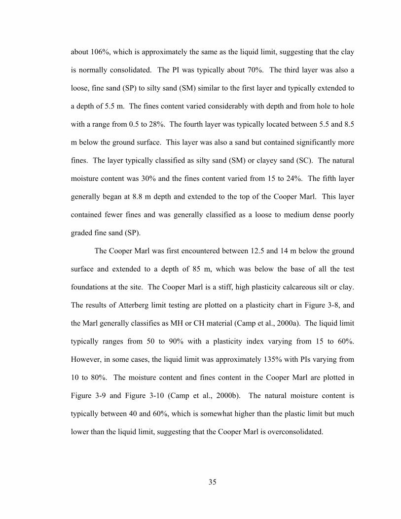
about 106%, which is approximately the same as the liquid limit, suggesting that the clay

is normally consolidated. The PI was typically about 70%. The third layer was also a

loose, fine sand (SP) to silty sand (SM) similar to the first layer and typically extended to

a depth of 5.5 m. The fines content varied considerably with depth and from hole to hole

with a range from 0.5 to 28%. The fourth layer was typically located between 5.5 and 8.5

m below the ground surface. This layer was also a sand but contained significantly more

fines. The layer typically classified as silty sand (SM) or clayey sand (SC). The natural

moisture content was 30% and the fines content varied from 15 to 24%. The fifth layer

generally began at 8.8 m depth and extended to the top of the Cooper Marl. This layer

contained fewer fines and was generally classified as a loose to medium dense poorly

graded fine sand (SP).

The Cooper Marl was first encountered between 12.5 and 14 m below the ground

surface and extended to a depth of 85 m, which was below the base of all the test

foundations at the site. The Cooper Marl is a stiff, high plasticity calcareous silt or clay.

The results of Atterberg limit testing are plotted on a plasticity chart in Figure 3-8, and

the Marl generally classifies as MH or CH material (Camp et al., 2000a). The liquid limit

typically ranges from 50 to 90% with a plasticity index varying from 15 to 60%.

However, in some cases, the liquid limit was approximately 135% with PIs varying from

10 to 80%. The moisture content and fines content in the Cooper Marl are plotted in

Figure 3-9 and Figure 3-10 (Camp et al., 2000b). The natural moisture content is

typically between 40 and 60%, which is somewhat higher than the plastic limit but much

lower than the liquid limit, suggesting that the Cooper Marl is overconsolidated.

35

The undrained shear strength is plotted as a function of elevation in Figure 3-11

(Camp et al., 2000b). The Marl is very stiff with undrained strengths typically ranging

from 100 to 200 kPa at the top of the layer and increasing with depth to a value between

200 and 300 kPa at a depth of about 45 m. Below this depth, the strength appears to

remain relatively constant. The results of the drained shear strength tests on the Cooper

Marl are plotted in the form of a p-q diagram in Figure 3-12 (Camp et al., 2000b). The

best-fit line through the data points indicates that the drained friction angle is

approximately 43° with relatively little variation about the line.

36

Figure 3-4 Boring log for test hole DS-1 (Hales 2003).

37

Figure 3-4 (Continued) Boring log for test hole DS-1.

38


39


40


41

Figure 3-5 Boring log for test hole MPS-11 (Hales 2003).

42

Figure 3-5 (Continued) Boring log for test hole MPS-11.

43

Figure 3-6 Boring log for test hole LB-28 (Hales 2003).

44

Figure 3-6 (Continued) Boring log for test hole LB-28.

45


46


47


48

0

5

10

15

20

Dep

th (m

)

Cooper Marl (CH)stiff to very stiffAvg. N=15, 40%<w<50%50%<LL<150%, 20%<PI<80%

Silty Sand (SM) and Clayey Sand (SC) Avg. N=7, w=30%

Sand (SP), fine, loose to medium dense, Avg. N=12

Sandy Clay (CH), soft, w=106, LL=104, PI-69

Sand (SP), loose, fine, Avg. N=6, 0.5 to 28% Fines

Sand (SP) to Silty Sand (SM), Loose, fine, Avg. N=5

Figure 3-7 Idealized soil profile for the Mt. Pleasant test site (Modified from Camp et al., 2000a).

49

Figure 3-8 Atterberg limits tests at various depths within the Cooper River Marl relative to the plasticity chart (Camp et al., 2000b).

Figure 3-9 Natural moisture content versus elevation in the Cooper River Marl (Camp et al., 2000b).

50

Figure 3-10 Fines content versus elevation in the Cooper River Marl (Camp et al., 2000b).

Figure 3-11 Undrained shear strength versus elevation from UU and CU triaxial shear test on undisturbed samples of the Cooper River Marl (Camp et al., 2000b).

51

Figure 3-12 Results of drained triaxial shear strength tests on Cooper River Marl plotted in a p-q diagram (Camp et al., 2000b).

3.5 In-Situ Testing

3.5.1 Standard Penetration (SPT) Testing

Standard penetration (SPT) testing was performed at many locations within the

sandy alluvial deposits above the Cooper Marl. Testing was performed by dropping a

622.75 N weight from a height of 0.762 m. The raw standard penetration value (N) is the

number of blows required to drive the split-spoon sampler through 0.3 m of penetration.

For test boring LB-28, the sampler was driven 0.6 m and the N value was taken from the

middle 0.3 of the interval. The (N1)60 value was determined using the equation

⎥⎦

⎤⎢⎣

⎡⎥⎦

⎤⎢⎣

⎡==

%60)(

5.0

'601applied

vo

acEn

EPqCNCN

σ (3-1)

52

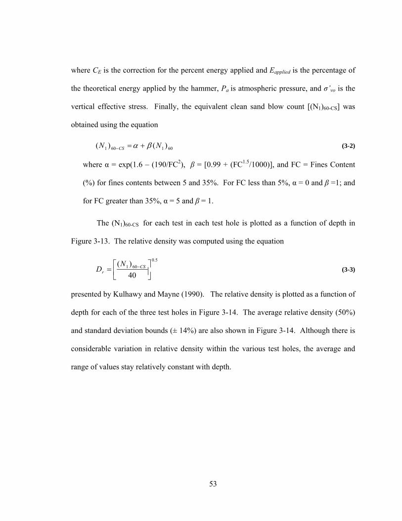
where CE is the correction for the percent energy applied and Eapplied is the percentage of

the theoretical energy applied by the hammer, Pa is atmospheric pressure, and σ’vo is the

vertical effective stress. Finally, the equivalent clean sand blow count [(N1)60-CS] was

obtained using the equation

601601 )()( NN CS βα +=− (3-2)

where α = exp(1.6 – (190/FC2), β = [0.99 + (FC1.5/1000)], and FC = Fines Content

(%) for fines contents between 5 and 35%. For FC less than 5%, α = 0 and β =1; and

for FC greater than 35%, α = 5 and β = 1.

The (N1)60-CS for each test in each test hole is plotted as a function of depth in

Figure 3-13. The relative density was computed using the equation

5.0601

40)(

⎥⎦

⎤⎢⎣

⎡= −CSr

ND (3-3)

presented by Kulhawy and Mayne (1990). The relative density is plotted as a function of

depth for each of the three test holes in Figure 3-14. The average relative density (50%)

and standard deviation bounds (± 14%) are also shown in Figure 3-14. Although there is

considerable variation in relative density within the various test holes, the average and

range of values stay relatively constant with depth.

53

0

2

4

6

8

10

12

14

16

18

0 10 20 30

(N1)60csDe

pth

(m)

LB-28DS-1MPS-11

Figure 3-13 Normalized SPT clean sand penetration resistance versus depth for three test holes near the test site.

54

Relative Density, Dr (%)

0

2

4

6

8

10

12

14

16

18

0 20 40 60 80 100D

epth

(m)

LB-28

DS-1

MPS-11

Mea

n

Mea

n - O

ne S

td. D

ev.

Mea

n +

One

Std

. Dev

.

Figure 3-14 Interpreted relative density versus depth based on SPT penetration resistance for three holes close to the test site.

55

3.5.2 Cone Penetration (CPT) Testing

Three cone penetration (CPT) soundings (MPS-7, LTB-1 and GT-1) were

performed at several locations near the test area, as shown in Figure 3-2. Two of the

soundings were performed by S&ME, while the third (GT-1) was performed by Georgia

Tech researchers. The CPT performed by S&ME used a track-mounted cone rig equipped

with an automated data acquisition system. The cone was a piezocone with a 10 cm2

surface area. The Georgia Tech cone rig used a small truck-mounted system with a

seismic piezocone with a 15 cm2 surface area. The porous filter for the both cones was

located in position 2, approximately 12 mm from the tip. The tests were conducted in

general accordance with ASTM D-3441. The soundings varied in depth from 13 to 30 m.

The normalized cone (tip) resistance (qc1), friction ratio (fr) and pore water

pressure (u) for each of the soundings are presented as a function of depth below the

ground surface in Figure 3-15 through Figure 3-17. The CPT results were used to

interpret the soil profile using the correlation with soil behavior type developed by

Robertson and Campanella (1988). The soil profile interpreted from the CPT soundings

is also shown for each sounding. Although the soil profile is generally similar for each

sounding and matches the idealized profile identified from the three test borings, there is

still considerable variation in the magnitude of tip resistance for the three soundings. The

presence of the clay layers in the profile is clearly indicated by a decrease in the tip

resistance, an increase in the friction ratio and an increase in the dynamic pore pressure

above the static pressure line (Uo). In addition to the clay layer between 1.5 and 3.5 m

and the Cooper Marl layer, the sand layer generally between 5.5 and 10 m appears to

56

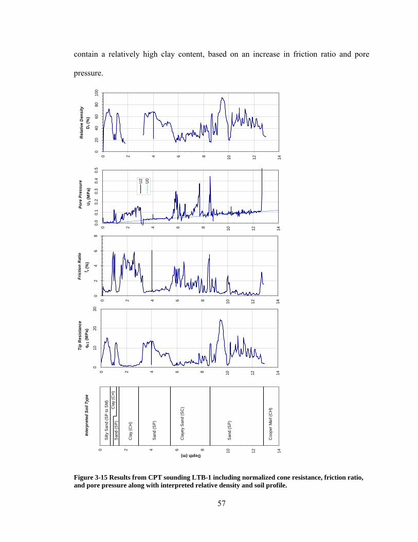
contain a relatively high clay content, based on an increase in friction ratio and pore

pressure. Fr

ictio

n R

atio

0 2 4 6 8 10 12 14

02

46

8

f r (%

)Ti

p R

esis

tanc

e

0 2 4 6 8 10 12 14

010

2030

q c1

(MPa

)Po

re P

ress

ure

0 2 4 6 8 10 12 14

0.0

0.1

0.2

0.3

0.4

0.5

U2 (

MPa

)

U2 U0

Rel

ativ

e D

ensi

ty

0 2 4 6 8 10 12 14

020

4060

8010

0

Dr (

%)

Inte

rpre

ted

Soil

Type

0 2 4 6 8 10 12 14

010

2030

Depth (m)

Coo

per M

arl (

CH)

Sand

(SP)

Cla

yey

Sand

(SC

)

Sand

(SP)

Cla

y (C

H)

Silty

San

d (S

P to

SM

)

Sand

(SP)

Cla

y (C

H)

Figure 3-15 Results from CPT sounding LTB-1 including normalized cone resistance, friction ratio, and pore pressure along with interpreted relative density and soil profile.

57

Fric

tion

Rat

io

0 5 10 15 20 25 30 35

02

46

8

f r (%

)

Tip

Res

ista

nce

0 5 10 15 20 25 30 35

010

2030

q c1

(MPa

)Po

re P

ress

ure

0 5 10 15 20 25 30 35

0.0

1.0

2.0

3.0

U (M

Pa)

U2

U0

Rel

ativ

e D

ensi

ty

0 5 10 15 20 25 30 35

020

4060

8010

0

Dr (

%)

Inte

rpre

ted

Soil

Type

0 5 10 15 20 25 30 35

010

2030

Depth (m)

Coo

per M

arl (

CH

)

Silt

y S

and

(SM

) and

C

laye

y S

and

(SC

)

San

d (S

P)

Cla

y (C

H)

San

d (S

P)

San

d (S

P) t

o S

ilty

San

d (S

M)

Figure 3-16 Results from CPT sounding MPS-7 including normalized cone resistance, friction ratio, and pore pressure along with interpreted relative density and soil profile.

58

Fric

tion

Rat

io

0 5 10 15 20 25 30 35

02

46

8

f r (%

)

Tip

Res

ista

nce

0 5 10 15 20 25 30 35

05

1015

20

q c1

(MPa

)Po

re P

ress

ure

0 5 10 15 20 25 30 35

0.0

1.0

2.0

3.0

4.0

U (k

Pa)

U2 U0

Rel

ativ

e D

ensi

ty

0 5 10 15 20 25 30 35

020

4060

8010

0

Dr (

%)

Inte

rpre

ted

Soil

Type

0 5 10 15 20 25 30 35

010

2030

Depth (m)

Coo

per M

arl (

CH)

Silty

San

d (S

M) a

nd

Cla

yey

Sand

(SC

)

San

d (S

P)

Cla

y (C

H)

San

d (S

P)

San

d (S

P) t

o Si

lty S

and

(SM

)

Figure 3-17 Results from CPT sounding GT-1 including normalized cone resistance friction ratio, and pore pressure along with interpreted relative density and soil profile.

59

Relative Density Based on CPT

The relative density (Dr) of the coarse-grained layers was estimated from the CPT

cone resistance using the equation

5.0

1

305

⎥⎥⎥⎥⎥

⎦

⎤

⎢⎢⎢⎢⎢

⎣

⎡⎟⎟⎠

⎞⎜⎜⎝

⎛

= a

c

r

pq

D (3-4)

developed by Kulhawy and Mayne (1990), where pa is atmospheric pressure, qc1 is the

cone resistance at a vertical effective stress of one atmosphere, and the sand is assumed to

be normally consolidated. The qc1 value is given by the equation

5.0

'1 ⎥⎦

⎤⎢⎣

⎡==

vo

acQcc

pqCqq

σ (3-5)

where σ’vo is the effective vertical stress and the adjustment factor CQ is less than or equal

to 1.7.

The friction angle in the granular layers was estimated using an equation

developed by Bolton (1986). The triaxial compression friction angle (φtc) is given by the

equation

rdcvtc I3+= φφ (3-6)

where φcv is the critical void ratio friction angle. Bolton (1986) recommends a value of

31 to 33 degrees for φcv in quartz sands with some silt and we have assumed a value of

31° in this study. Ird is given by the equation

60

1100ln10 −⎥⎥⎦

⎤

⎢⎢⎣

⎡

⎥⎥⎦

⎤

⎢⎢⎣

⎡⎟⎟⎠

⎞⎜⎜⎝

⎛−=

a

frrd p

pDI (3-7)

where pf is the mean effective stress at failure. Horizontal pressures at the failure state

were estimated using Rankine values for active and passive pressures.

The relative density and friction angle versus depth profiles computed using

Equation 3.4 and Equation 3.6, respectively, are shown for each test hole in Figure 3-18.

There is a substantial variation in relative density and friction angle in the surface sand

layer; however, in the sand layer immediately below the surface clay, there appears to be

reasonable agreement. In this fine sand layer, the relative density is approximately 50%

with a friction angle of 38°. In the underlying silty to clayey sand, the relative density

and friction angle drop significantly relative to the cleaner sand above, and the variability

also increases. In this clayey sand layer, the relative density appears to vary from 20 to

50% with an average of about 40%, while the friction angle generally varies from 31° to

35° with an average of about 33°. In the lowest fine sand layer, the interpreted values are

once again more consistent. The average relative density is about 50% with a friction

angle of 3l.5°.

61

Interpreted Soil Type

0

5

10

15

0 10 20 30

Dep

th (m

)

Cooper Marl (CH)

Silty Sand (SM) and Clayey Sand (SC)

Sand (SP)

Clay (CH)

Sand (SP)

Sand (SP) to Silty Sand (SM)

Relative Density

0

5

10

15

0 20 40 60 80 100

Dr (%)

MPS-7GT-1LTB-1

Friction Angleφ ( degrees)

0

5

10

15

30 32 34 36 38 40 42 44

MPS-7GT-1LTB-1

Figure 3-18 Interpreted Relative density and friction angle versus depth for sand layers in the soil profile based on three CPT soundings.

Undrained Shear Strength Interpretation Based on CPT

The undrained shear strength of the fine-grained layers in the profile was

estimated from the CPT cone tip resistance using the equation

⎟⎟⎠

⎞⎜⎜⎝

⎛ −=

k

ocu N

qS

σ (3-8)

where qc is cone tip resistance, σo is the total vertical stress, and Nk is the bearing capacity

factor for an electric piezocone. According to Robertson and Campanella (1988), the Nk

value typically ranges from 10 to 20 and was assumed to be equal to 15 for this study.

Although the undrained shear strength obtained from Figure 3-19 is only an estimate, the

62

Interpreted Soil Type

0

5

10

15

20

25

30

35

0 10 20 30D

epth

(m) Cooper Marl (CH)

Silty Sand (SM) and Clayey Sand (SC)

Sand (SP)

Clay (CH)

Sand (SP)

Sand (SP) to Silty Sand (SM)

Undrained StrengthSu (kPa)

0

5

10

15

20

25

30

35

0 100 200 300 400 500

MPS-7GT-1LTB-1

Figure 3-19 Interpreted Undrained shear strength versus depth for clay layers in the soil profile based on three CPT soundings.

approach does provide a continuous profile that shows the consistency of the strength

within layers in the profile. The undrained shear strength computed using Equation 3-8 is

shown as a function of depth in Figure 3-19. The undrained strength in the upper clay

layer ranges from 25 to 50 kPa and tends to increase with depth. The estimated

63

undrained strength in the Cooper Marl also tends to increase with depth with an average

strength of about 125 kPa at the top of the layer and about 275 kPa at the bottom. This

trend and the strength values shown in Figure 3-19 are generally in good agreement with

the measured undrained shear strength from laboratory tests shown in Figure 3-11.

Shear Wave Testing

The shear wave velocity (Vs) profile was measured during two seismic cone

penetrometer (SCPT) soundings (MPS-7 and GT-1), which were described previously,

and one conventional down-hole test performed in test hole DS-1 by Bruce Redpath of

Redpath Geophysics. The shear wave velocity was normalized for overburden pressure

(Vs1) using the equation

25.0

'11

⎟⎟⎠

⎞⎜⎜⎝

⎛=

oss VV

σ (3-9)

The shear wave velocity profiles obtained from the two SCPT tests and the downhole test

are provided in Figure 3-20. Figure 3-20 (a) presents the Vs results, while (b) presents

Vs1 to a depth of 30 m. The agreement between the three tests is relatively good. In

some cases where discrepancies occur, the source appears to be an over-estimate of

velocity at one depth followed by an underestimate at the subsequent depth, so that the

average is about the same as in the other tests. In many cases, the Vs1 value is greater

than 200 m/sec, indicating that the sand is not susceptible to liquefaction; however, the

SPT and CPT values indicate that liquefaction is likely to occur, as discussed

subsequently. The Vs value in the Marl is higher than in the overlying sands and

increases progressively from 335 m/sec at the top of the layer to 762 m/sec at the base.

However, when the correction is applied to get Vs1, the velocity in the Marl remains

64

nearly constant, suggesting that the material properties remain essentially constant with

depth.

Shear Wave VelocityV s (m/s)

0

5

10

15

20

25

30

35

0 200 400 600 800 1000

GT

LTB-1

Redpath

Shear Wave VelocityV s1 (m/s)

0

5

10

15

20

25

30

35

0 200 400 600

GT

LTB-1

Redpath

Figure 3-20 Profiles of Vs and Vs1 versus depth based on down SCPT sounding and a down-hole shear wave velocity test conducted by Redpath Geophysics.

3.6 Liquefaction Hazard Analysis

On August 31, 1886 a major earthquake struck Charleston, South Carolina.

Because no instrumental records are available, it is not possible define the magnitude and

peak acceleration precisely, however, Bollinger (1977) has assigned a magnitude of 7.3

65

and an intensity of X on the modified Mercalli scale to the event. The earthquake caused

an estimated $5 to $6 million damage to buildings, (see damage in Figure 3-21), as well

as liquefaction in the subsurface materials (Stover and Coffman, 1993). A photo of a

large sand boil produced by liquefaction during the 1886 earthquake is shown in Figure

3-22. For an excellent compilation of first-hand observations of the 1886 Charleston

earthquake, the reader is referred to Peters and Herrmann (1986). The new Ravenel

Bridge has been designed to withstand an earthquake magnitude similar to the earthquake

that struck the area in 1886, as well as smaller events which might occur more frequently.

Despite research by a number of investigators, the exact fault mechanism

responsible for the 1886 Charleston earthquake is still not known. Because there was no

surface manifestation of the fault, geophysical techniques have been employed to identify

potential faults; however, no consensus has developed within the scientific community

regarding the causative fault. Instead, a number of areal source zones have been

developed to quantify the earthquake hazard (Elton and Hadj-Hamou, 1990).

Based on these source zones, the U.S. Geological Survey has developed

probabilistic ground motion estimates for the Charleston area (Frankel et al., 2000).

Maps are available for acceleration levels corresponding to 2%, 5%, and 10%

probabilities of exceedance in 50 years. These acceleration levels correspond to return

periods of approximately 2500, 1000 and 500 years. For the design of bridges in South

Carolina, the South Carolina Department of Transportation requires a two level design

approach. For more frequent small to moderate earthquakes, bridges are designed so that

the bridge will remain essentially elastic and can remain in full service with little if any

damage. For this first-level event, known as the Functional Evaluation Earthquake

66

(FEE), the peak ground acceleration values are associated with a 10% probability of

exceedance in 50 years. The bridge is also designed for a major earthquake, known as

the Safety Evaluation Earthquake (SEE). This earthquake is used to ensure that the

structure does not collapse and that there is no loss of life. In addition, for critical

bridges, service should be maintained and damage should be easily detectable and

repairable. The acceleration level for the SEE event is associated with a 2% probability

of exceedance in 50 years.

According to the US Geological Survey, the peak ground acceleration at the

bridge site with a 2% probability of exceedance in 50 years is 0.77g and is associated

with a modal magnitude 7.3 earthquake. The peak ground acceleration at the bridge site

with a 10% probability of exceedance in 50 years is 0.16g and is associated with a modal

magnitude 6.4 earthquake.

A liquefaction analysis has been performed for the two earthquake levels

described previously. The analyses were performed in accordance the recent

recommendations of the MCEER workshop (Youd et al., 2001). The analyses were

performed using the CPT sounding identified as GT-1. The results of the analysis for the

M7.3 and 0.77g event are shown in Figure 3-23. For this relatively large event, the

analyses indicate that essentially all of the profile above the Cooper Marl would liquefy,

with the exception of the clay layer in the upper part of the soil profile. Despite the high

fines content in the clayey sand layer, liquefaction would also be expected in this layer.

The results of the analysis for the M6.4, 0.16g event are shown in Figure 3-24.

For this relatively small event, the analyses indicate that most of the sand above the

Cooper Marl would not liquefy. Additional analyses, not shown here, indicate that this

67

event represents the upper bound for which liquefaction does not occur. If the

acceleration or earthquake magnitude is any higher, then the entire sand layer above the

Cooper Marl liquefies.

In contrast, liquefaction analyses based on the shear wave velocity indicate that

liquefaction would unlikely occur in the zone from 5 to 13 m below the ground surface

because the shear wave velocity is greater than 215 m/sec.

Figure 3-21 Photograph of a brick house wrecked by the Charleston earthquake of August 31, 1886 (USGS, 2005).

68

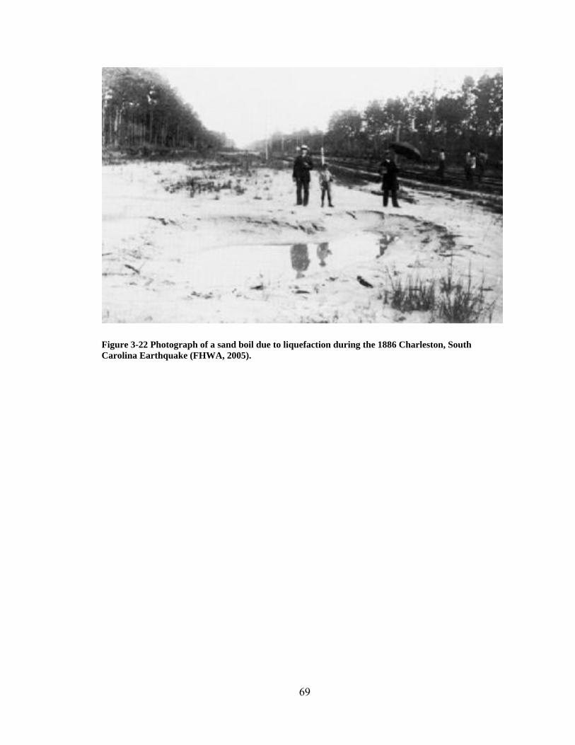
Figure 3-22 Photograph of a sand boil due to liquefaction during the 1886 Charleston, South Carolina Earthquake (FHWA, 2005).

69

0

2

4

6

8

10

12

14

16

18

20

22

24

26

28

30

0 1 2 3 4

SBT Index

0

2

4

6

8

10

12

14

16

18

20

22

24

26

28

30

0 10 20 30

Tip Resistance (MPa)R

elat

ive

Dep

th (m

)0 1

-0.16

-10.17

-20.18

-30.18

-40.19

-50.2

-60.2

-70.21

-80.22

-90.22

F.S. Against Liquefaction

2

Figure 3-23 Profiles showing cone tip resistance, SBT index, and factor of safety against liquefaction versus depth for GT-1 due to M7.3 earthquake producing 0.77 g peak acceleration associated with a 2% probability of exceedance in 50 years. (Hales, 2003)

70

0

2

4

6

8

10

12

14

16

18

20

22

24

26

28

30

0 1 2 3 4

SBT Index

0

2

4

6

8

10

12

14

16

18

20

22

24

26

28

30

0 10 20 30

Tip Resistance (MPa)

Rel

ativ

e D

epth

(m)

0 1 2-0.16

-10.17

-20.18

-30.18

-40.19

-50.2

-60.2

-70.21

-80.22

-90.22

F.S. Against Liquefaction

Figure 3-24 Profiles showing cone tip resistance, SBT index, and factor of safety against liquefaction versus depth for GT-1 due to M6.4 earthquake producing 0.16 g peak acceleration associated with a 10% probability of exceedance in 50 years. (Hales 2003)

71

4 Test Set-Up and Pile Description

4.1 Introduction

Three successively larger lateral statnamic load tests were performed on the pile

designated MP-3 on August 29, 2000, each about one hour apart. This testing was

performed as part of the design phase for the replacement bridge for the Cooper River

Bridge. Embedded or down-hole charges were used to induce high excess pore water

pressure, causing liquefaction of the soil directly surrounding the test site. The following

chapter provides an overview of the foundation construction, foundation properties,

statnamic load test configuration, and the test layout.

4.2 Pile Description

According to the testing report (Brown, 2000), the construction of the pile

numbered MP-3 was finished on July 29, 2000. The consulting engineer on the project

was S & ME, Inc. The test foundation was a reinforced concrete shaft with a permanent

steel liner, also known as cast-in-steel-shell (CISS) pile. The outside diameter of the steel

shell was 2.59 m with a wall thickness of 25.4 mm and extended to a depth of about

20.12 m below the ground surface. After the steel casing was installed using a vibratory

hammer, the inside was drilled out and advanced to a final depth of 31.7 m prior to

73

pouring the reinforced concrete core. Figure 4-1 shows the drilling process used to

construct MP-3.

Figure 4-1 Contractor used a track-mounted SoilMec for drilling (photograph from a presentation by the SCDOT and S&ME to the CE Club).

The average 30-day compressive strength of the concrete placed in the steel shell

of MP-3 was 42.7 MPa (6.2 ksi) based on six laboratory-cured samples. The vertical

reinforcement consisted of 36 #18 bars evenly spaced around a ring with a diameter of

2.14 m. Number 6 bar spiral reinforcement was used as the containment reinforcement

with a pitch of 89 mm. A 150 mm cover was maintained between the spiral

reinforcement and the inside of the steel casing. Figure 4-2 provides a photograph of the

reinforcement cage construction for MP-3.

74

Figure 4-2 Photograph of worker assembling reinforcement cage at the Mount Pleasant site (photograph from a presentation by the SCDOT and S&ME to the CE Club).

The steel casing was installed with a stick-up height of 2.13 m above the ground

surface and extended to 20.12 m below the ground surface. After the installation of the

steel shell, the verticality of the shaft was assessed by Trevi Icos Corporation. The test

shaft was actually tilted about 1.1 degrees from vertical to the North-East. A drawing of

the measured shaft alignment is presented in the Appendix. The concrete portion of the

test shaft was then installed with a stick-up height of 1.83 m above the ground surface

and extended to a depth of 31.7 m below ground. Figure 4-43 presents the pile

dimensions. Figure 4-5 shows the drilled shaft together with the idealized soil profile.

75

Figure 4-3 Drilled shaft dimensions, strain gauges, and accelerometers.

Figure 4-4 Drilled shaft dim

ensions, strain gauges, and accelerometers.

76

Figure 4-5 Drilled shaft and corresponding soil profile.

4.3 Test Set-Up

The lateral load was applied with a statnamic device on a sled. Figure 4-6

provides a schematic of the test set up. The sled has a series of donut shaped weights that

encase a core called the silencer cylinder. The vertical lines on the statnamic device

schematic are the separate weights that give the device its mass and in turn its force. The

statnamic sled, which weighs approximately 9.07 X 104 kg, was supported by a steel

trestle with a timber crane mat deck. The trestle was supported by driven H-piles. The

load was applied about 1.31 m above the ground surface through a hemispherical bearing

77

to allow rotation of the shaft, ensuring a free-head condition. A load cell at the point of

load application was used to directly measure applied force.

Figure 4-6 Schematic of statnamic load test at the Mt. Pleasant site (drawing modified from the Ravenel Bridge Project Load Test Plans).

78

4.4 Above Ground Instrumentation

Two 0.76 m linear variable differential transducers (LVDT) were installed to

directly measure the pile head deflection, one above the load point and the other below it.

The LVDTs were mounted on an independent reference beam supported by driven piles

within isolation casings. The top LVDT was mounted 1.65 m above the ground surface;

the lower LVDT was located 1.1 m above the ground surface.

Two accelerometers were mounted at the height of the load point on the opposite

side of the load application. One of these accelerometers failed to give reliable readings,

so the data was not used for analysis. Two more accelerometers were mounted above

ground. The first was mounted above the load point at a height of 1.89 m. The other was

mounted on the reference beam to detect any significant movement of the structure that

could affect the LVDT data. The location of the instrumentation is shown in Figure 4-7.

79

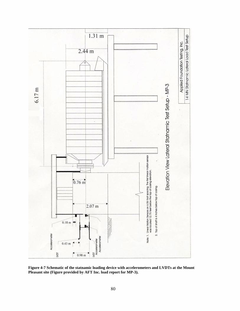
Figure 4-7 Schematic of the statnamic loading device with accelerometers and LVDTs at the Mount Pleasant site (Figure provided by AFT Inc. load report for MP-3).

80

4.5 Below Ground Instrumentation

A series of eight accelerometers or Down-hole Lateral Motion Sensors (DLMS)

were installed with individual guide mounts that were lowered into a grooved

inclinometer casing that was pre-cast into the test shaft. The accelerometers were

installed to measure lateral motion in the direction of the load test. The accelerometers

were placed at the following elevations (meters below the ground surface): 1.83, 3.83,

5.83, 7.83, 9.83, 11.52, 13.22, 14.91 as shown in Figure 4-43.

Strain gauges were also installed a ten depth stations to measure the bending in

the pile. Resistance-type strain gauges were mounted on a separate rebar consisting of a

4 foot long #4 bar tied to the rebar cage before installation. For the first 5 stations two

gauges placed in line with the direction of loading with a horizontal distance between

gauge pairs of 2.14 m. For stations 6-10, an additional two strain gauges were placed

perpendicular to the direction of load application and similarly spaced. The depths and

layout of the strain gauges are shown previously in Figure 4-43.

All of the data (load, deflection, acceleration, and strain) were collected using a

Megadac® data acquisition system at a sampling rate of 2000 samples per second for

each channel. A pre-trigger of 0.5 seconds before the loading was used to start recording

the data while a 5 second post-trigger was used to terminate data acquisition.

Piezometers were installed in the ground around the test shaft to quantify the pore

water pressure increase induced by the explosive charges, along with subsequent

dissipation of pore pressure. Plan and profile views of the piezometer layout relative to

the test shaft and the explosive charges are presented in Figure 4-9 and Figure 4-10,

respectively. The transducers were basically arranged to produce three vertical arrays of

81

sensors at radial distances of 1.83, 7.32, and 10.36 m from the center of the test shaft.

The vertical arrays were typically spaced at about 1.5 m depth intervals. The piezometer

number and depth below ground surface is indicated in this figure.

Figure 4-8 Reinforcement cage after installation of strain gages and inclinometers (photograph from a presentation by the SCDOT and S&ME to the CE Club).

The piezometers labeled with a “B” designation consisted of piezoresistive

transducers designed to withstand transient blast pressures of up to 41 MPa (6000 psi)

while still resolving the residual pore pressure to within ±0.0007 MPa (0.1 psi). The

transducers with an “A” designation consisted of electrical resistance transducers with a

resolution of 6.9 kPa (1 psi) when used in conjunction with the Megadac® data collection

system. The A-type transducers experienced an unusually high failure rate during field

testing and typically only provided marginally useful data; however the B-type sensors

generally performed well.

82

BYU Piezometer

AFT Piezometer

Blast Holes

Load Direction

Inner Ring1.83 m R

Middle Ring7.32 m R

Outer Ring10.36 m R

A5? m

B156.40m

A41.83m

B143.35m

A34.88m A2

10.67m

B137.93m

B126.40m

B103.35m B9

4.88m A110.06m

B111.89m

B210.67m

B36.40m

B43.20m

B51.83m

3.96 m R

4.57 m R

5.18 m R

B64.88m

B77.93m

B810.98m

B111.83m

MP-3

Figure 4-9 Plan view of the piezometers and charges (Brown, 2000).

83

Figure 4-10 Elevation view showing a profile of piezometers and down-hole charges relative to the test shaft.

4.6 Blast Layout

Liquefaction is manifest by an increase in pore water pressure. This increase in

pore water pressure was achieved by detonating explosive charges distributed around

MP-3 test shaft. A pilot liquefaction test was performed at a location separate from the

test site for MP-3. The pilot test was done to better define the charge weight, spacing,

and delay sequence so as to fully liquefy the soil around the test shaft. For each of the

84

load tests, eight charges spaced evenly around three different radii were detonated. The

first eight blast holes were spaced around a radius of 3.96 m. The second and third blast

rings radii were 4.57 m and 5.18 m. The charges were staggered to help avoid

sympathetic detonations. The first blast series set a 0.68 kg (1.5 lb) charge at 3.05, 6.1,

9.14, and 11.73 m below the ground surface. The second blast series used 0.91 kg (2 lb)

charges at 4.57, 7.62, and 10.67 m depths. The third and final blast series put 0.68 kg

(1.5 lb) charges at the same depths as in the first blast series. This layout can be seen in

Figure 4-9 and Figure 4-10. Even though the charges were staggered, some sympathetic

blasts still occurred during the second blast series at 9.14 and 11.73 m depths.

The binary explosives consisted of a mixture of ammonium nitrate and nitro-

methane, and the weights are given in equivalent weights of TNT. During each of the

three blast sequences, the charges were detonated two at a time with a delay of 250 msec

between detonations. The charges were detonated beginning around the bottom ring and

then moved upward around each subsequent ring to the top.

85

5 Statnamic Lateral Load Test Results

5.1 Introduction

To determine the effects of liquefaction on the lateral resistance of deep

foundations, dynamic lateral load tests were performed on August 29, 2000. Three lateral

load tests were performed with a statnamic load sled. With each test, the load was

progressively increased. Before each test, a set of down-hole explosives was detonated to

increase the pore water pressure in the soil to induce liquefaction. The planned order of

the load tests went as follows:

1. Detonate the embedded charges to liquefy the soil.

2. Wait about 45 seconds for dissipation of gasses from the explosions.

3. Fire the statnamic device.

After each detonation of the down-hole charges and loading, there was evidence of sand

boils and water pressure venting at the ground surface around the test site. Some settling

also occurred after each test. After the third test was completed, the maximum surface

elevation change was more then a quarter of a meter (see Appendix A). During the three

lateral load tests, the maximum deflection obtained was more than 98 mm, and the largest

load used was more than 6500 kN. Data was recorded for more then 8 seconds for all

three tests. Analysis of the data yielded no significant deflections after about 1.5 seconds

following the test firing; therefore the data was truncated at this point, and all the analysis

87

of the data was done in that amount of time. The results of the three tests are described in

the following sections of this chapter.

5.2 Lateral Load Tests

5.2.1 First Lateral Load Test

The first lateral load test, as was mentioned in chapter 4, had two LVDTs that

measured the pile head deflection, one above the load point and one below. Since the

actual deflection at the load point wasn’t measured, linear interpolation was used to

determine the deflection at the load point. There is some potential for error because of

this linear assumption, but since the distance between the two LVDTs is very small, the

error should be negligible. The time histories of the upper and lower LVDT deflections

are presented in Figure 5-1. As shown in Figure 5-2, a maximum load of 4500 kN was

achieved, and the maximum deflection attributed to that load was 59.6 mm for the first

test.

During the first lateral load test there seemed to be some high frequency

vibrations or “noise.” These vibrations can be seen in the load-time history just after 0.5

seconds in Figure 5-2. This noise is thought to be created by the initial reaction of the

donut weights around the silencer cylinder. No matter how much the weights are pushed

together, inevitably some slack persists. When the load is applied, this slack is

eliminated, which causes the weights to impact the system, initially inducing these high

frequency vibrations. Puffs of dust from in-between the load weights were also noticed

just after the load was applied, evidence of slack that needed to be removed. The load

88

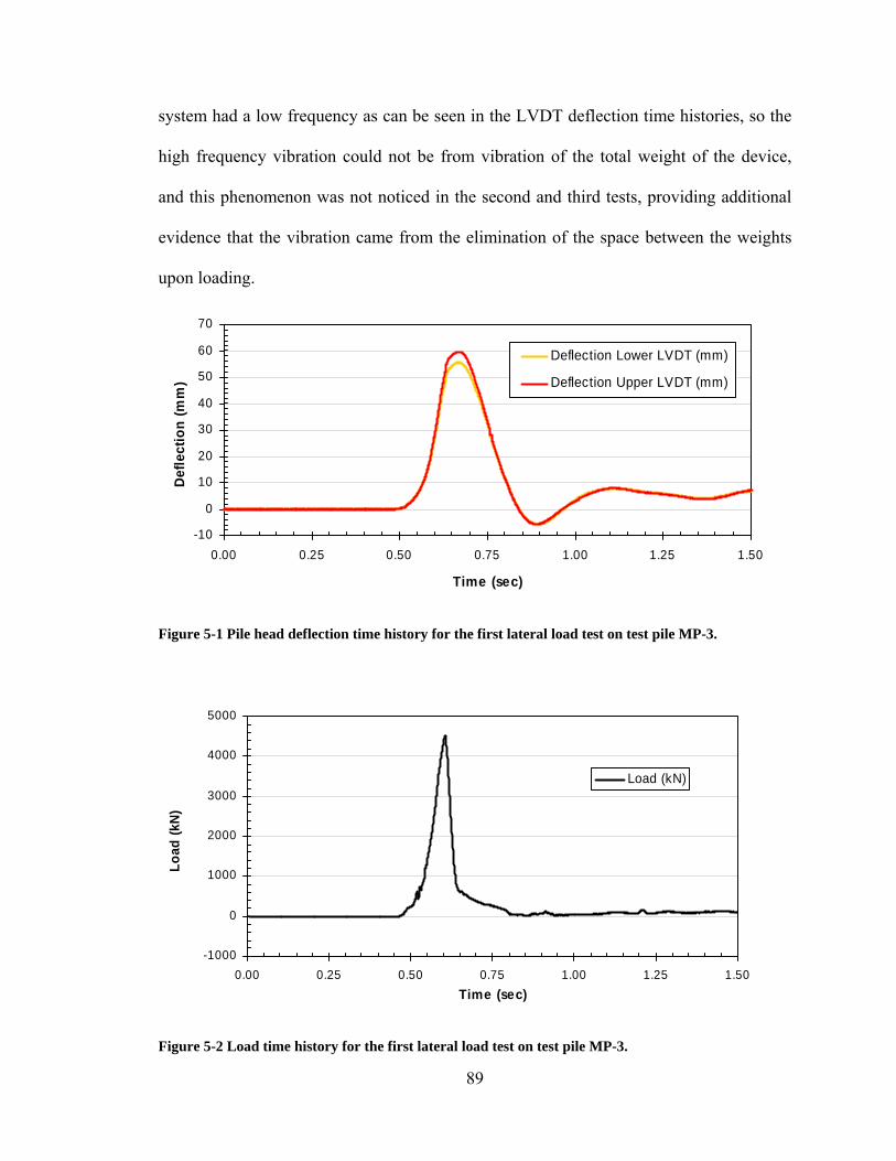
system had a low frequency as can be seen in the LVDT deflection time histories, so the

high frequency vibration could not be from vibration of the total weight of the device,

and this phenomenon was not noticed in the second and third tests, providing additional

evidence that the vibration came from the elimination of the space between the weights

upon loading.

-10

0

10

20

30

40

50

60

70

0.00 0.25 0.50 0.75 1.00 1.25 1.50

Time (sec)

Def

lect

ion

(mm

)

Deflection Lower LVDT (mm)

Deflection Upper LVDT (mm)

Figure 5-1 Pile head deflection time history for the first lateral load test on test pile MP-3.

-1000

0

1000

2000

3000

4000

5000

0.00 0.25 0.50 0.75 1.00 1.25 1.50Time (sec)

Load

(kN

)

Load (kN)

Figure 5-2 Load time history for the first lateral load test on test pile MP-3.

89

-500

0

500

1000

1500

2000

2500

3000

3500

4000

4500

5000

-10 0 10 20 30 40 50 60

Deflection (mm)

Load

(kN)

Figure 5-3 Load versus deflection curve for load test 1 on test pile MP-3.

5.2.2 Second Lateral Load Test

The second load test data was a little cleaner, since the statnamic device had

already been fired. In the second and third load tests the high frequency vibration is not

evident in either the load or acceleration time histories. The LVDT deflections were

zeroed using the average deflection obtained from the first thirty points of the first load

test’s LVDT data to maintain the residual deflections from that first test that were present

at the start of the second test. In contrast to the deflection, the load at the beginning of

each load test should be zero. Therefore, the load data were zeroed using the average of

the first thirty points of the load. The maximum load obtained in the second test was

almost 5500 kN and the maximum deflection caused by this load was 87.4 mm. The

deflection and load time histories for the second test are plotted in Figure 5-4 and Figure

5-5, respectively, while the load-deflection curve is plotted in Figure 5-6.

90

-20

0

20

40

60

80

100

0.00 0.25 0.50 0.75 1.00 1.25 1.50

Time (sec)

Def

lect

ion

(mm

)Deflection Lower LVDT (mm)


Figure 5-4 Pile head deflection time history for the second lateral load test on test pile MP-3

-1000

0

1000

2000

3000

4000

5000

6000

0.00 0.25 0.50 0.75 1.00 1.25 1.50Time (sec)

Load

(kN)

Load (kN)

Figure 5-5 Load time history for the second lateral load test on test pile MP-3.

91

-1000

0

1000

2000

3000

4000

5000

6000

-10 0 10 20 30 40 50 60 70 80 9

Deflection (mm)

Load

(kN)

0

Figure 5-6 Load versus Deflection for load test 2.

5.2.3 Third Lateral Load Test

The third load test data was zeroed in the same manner as was the second load

test. The maximum load that the statnamic device delivered was just over 6500 kN, and

the resulting peak deflection was 98.0 mm. The deflection and load time histories for the

third test are plotted in Figure 5-7 and Figure 5-8, respectively, while the load-deflection

curve is plotted in Figure 5-9.

92

-20

0

20

40

60

80

100

0.00 0.25 0.50 0.75 1.00 1.25 1.50

Time (sec)

Defle

ctio

n (m

m)

Deflection Lower LVDT (mm)


Figure 5-7 Pile head deflection time history for the third lateral load test on test pile MP-3.

-1000

0

1000

2000

3000

4000

5000

6000

7000

0.00 0.25 0.50 0.75 1.00 1.25 1.50

Time (sec)

Load

(kN)

Load (kN)

Figure 5-8 Load time history for the third lateral load test on test pile MP-3.

93

-1000

0

1000

2000

3000

4000

5000

6000

7000

-20 0 20 40 60 80 100

Deflection (mm)

Load

(kN

)

Figure 5-9 Load versus Deflection curve for load test 3.

5.3 Pile Motion from Acceleration Data

The eight DLMSs or the downhole accelerometers can be used to determine

acceleration, velocity and deflections along the length of the pile. To derive the velocity

and displacement from the acceleration, the acceleration needed to be zeroed to start with

no motion, as was true with the test. A baseline correction was also necessary to adjust

for the small drift in the accelerometer during the test. Although the drift in baseline

acceleration is very small, drift in the accelerometer during the test can still lead to

unrealistic displacements after double integration over the time history. Baseline

correction has been used widely in the arena of earthquake engineering to adjust the

accelerations obtained from their instruments. A program called Baseline (Gregor, 2001)

was used to baseline correct the accelerations. This program performed a least squares

inversion between an input deflection time history and an nth degree polynomial. The

94

accelerations could then be integrated with respect to time to derive the velocities, and

again to get the deflections. These deflections were then compared to the LVDT

deflections to ensure that the baseline correction was reasonable. The accelerometer

attached to the reference frame showed very small movements, so small that they were

considered insignificant for all three load tests.

All of the acceleration, velocity, and deflection graphs show that the peak velocity

occurs where the acceleration is zero, and the velocity is zero when the deflection is at its

maximum as expected by calculus. This correlation between acceleration, velocity, and

deflection is a good indication the accelerations were properly integrated.

On the acceleration graphs the maximum values always occur as negative. As the

pile is loaded, it has to push the soil out of the way. In the unloading portion of the

graphs the gap the pile produced allows it to travel more freely causing the accelerations

to be greater.

The peak accelerations for all three tests are greater than those seen during an

earthquake, but this isn’t a problem since the inertial force can easily be removed from

the measured force. Typical accelerations seen during an earthquake might range from

0.3 g to 1.3 g. The peak velocities however, are values similar to those seen during

earthquakes, considering an average velocity from an earthquake is about 1 m/s/g.

Therefore, the acceleration to which this loading corresponds to can be calculated based

on the measured velocity. Also since velocity is proportional to the damping force, the

damping for this test is likely to be similar to what is expected in an earthquake.

95

5.3.1 First Load Test Pile Motion from Acceleration Data

Figure 5-10 through Figure 5-13 show the measured acceleration, and derived

velocity and deflection time histories from each accelerometer location along the length

of the test pile for the first load test. Almost all the accelerometers worked during the

test; however, one accelerometer malfunctioned at the load point. Since two

accelerometers were placed at that location, an acceleration time history was still

recorded. They can be seen in Figure 5-10b.

Figure 5-14 through Figure 5-16 show acceleration, velocity, and deflection

versus depth profiles at several selected time steps to provide an idea of the pile motion

during each test. The deflections from the two LVDTs are plotted along with the

acceleration-derived deflections in Figure 5-16. In general, the computed deflections

agree reasonably well with the LVDT deflections, however. The main source of error is

most likely from baseline correction of the accelerations.

96

-40

-25

-10

5

20

35

50

65

0 0.25 0.5 0.75 1 1.25 1.5Time (sec)

Acc

eler

atio

n &

D

efle

ctio

n

-0.7

-0.4

-0.1

0.2

0.5

0.8

1.1

Vel

ocity

Acceleration (m/s^2)Deflection (mm)Velocity (m/s)

(a) 1.89 m (6.2 ft) above ground

-40

-25

-10

5

20

35

50

65

0 0.25 0.5 0.75 1 1.25 1.5Time (sec)

Acc

eler

atio

n &

D

efle

ctio

n

-0.7

-0.4

-0.1

0.2

0.5

0.8

1.1

Vel

ocity


(b) 1.31 m (4.3 ft) above ground

Figure 5-10 Acceleration, velocity, and deflection graphs from test 1 accelerometers.

97

-40

-25

-10

5

20

35

50

65

0 0.25 0.5 0.75 1 1.25 1.5

Time (sec)

Acce

lera

tion

& De

flect

ion

-0.7

-0.4

-0.1

0.2

0.5

0.8

1.1

Vel

ocity


(a) 1.83 m (6.0 ft) below ground

-40

-25

-10

5

20

35

50

65

0 0.25 0.5 0.75 1 1.25 1.5

Time (sec)

Acce

lera

tion

& De

flect

ion

-0.7

-0.4

-0.1

0.2

0.5

0.8

1.1

Velo

city


(b) 3.83 m (12.56 ft) below ground

-40

-25

-10

5

20

35

50

65

0 0.25 0.5 0.75 1 1.25 1.5

Time (sec)

Acce

lera

tion

& De

flect

ion

-0.7

-0.4

-0.1

0.2

0.5

0.8

1.1Ve

loci

ty


(c) 5.83 m (19.12 ft) below ground

Figure 5-11 (Continued) Acceleration, velocity, and deflection graphs from test 1 accelerometers.

98

-40

-25

-10

5

20

35

50

65

0 0.25 0.5 0.75 1 1.25 1.5

Time (sec)

Acc

eler

atio

n &

D

efle

ctio

n

-0.7

-0.4

-0.1

0.2

0.5

0.8

1.1

Velo

city



-40

-25

-10

5

20

35

50

65

0 0.25 0.5 0.75 1 1.25 1.5

Time (sec)

Acce

lera

tion

& De

flect

ion

-0.7

-0.4

-0.1

0.2

0.5

0.8

1.1

Velo

city



-40

-25

-10

5

20

35

50

65

0 0.25 0.5 0.75 1 1.25 1.5Time (sec)

Acc

eler

atio

n &

De

flect

ion

-0.7

-0.4

-0.1

0.2

0.5

0.8

1.1

Vel

ocity


(c) 11.52 m (37.8 f t) below ground

Figure 5-12 (Continued) Acceleration, velocity, and deflection graphs from load test 1 accelerometers.

99

-40

-25

-10

5

20

35

50

65

0 0.25 0.5 0.75 1 1.25 1.5

Time (sec)

Acce

lera

tion

& De

flect

ion

-0.7

-0.4

-0.1

0.2

0.5

0.8

1.1

Vel

ocity




-4

-2

0

2

4

6

8

10

12

14

16

-40 -30 -20 -10 0 10 20

Acceleration (m/s^2)

Dep

th B

elow

Gro

und

(m)

0.5 sec0.55 sec0.575 sec0.6 sec0.625 sec0.65 sec0.85 sec0.90 sec

Figure 5-14 Acceleration versus depth plots plot at several times for load test 1.

100

-4

-2

0

2

4

6

8

10

12

14

16

-0.4 -0.2 0 0.2 0.4 0.6 0.8 1

Velocity (m/s)

Dep

th B

elow

Gro

und

(m)


Figure 5-15 Velocity versus depth plots derived from accelerations at several times for load test 1.

-4

-2

0

2

4

6

8

10

12

14

16

-20 0 20 40 60 80

Deflection (mm)

Dep

th B

elow

Gro

und

(m)

0.5 sec0.55 sec0.575 sec0.6 sec0.625 sec0.65 secLVDTs0.85 sec0.9 sec

Figure 5-16 Deflection versus depth plots derived from accelerations at several times for load test 1 along with measured deflections from LVDTs above ground.

101

5.3.2 Second Load Test Pile Motion from Acceleration Data

The acceleration data recorded for this test can be found in Figure 5-17. Attempts

to baseline correct the acceleration data for the second test was much more difficult

because of some residual deflection present at the beginning of the load test. All the

corrected accelerations for the test start out at zero but catch up to the actual deflections

before they reach their peak.

102

-60

-40

-20

0

20

40

60

80

100

0 0.25 0.5 0.75 1 1.25 1.5Time (sec)

Acce

lera

tion

& De

flect

ion

-0.9

-0.6

-0.3

0

0.3

0.6

0.9

1.2

1.5

Vel

ocity



-60

-40

-20

0

20

40

60

80

100

0 0.25 0.5 0.75 1 1.25 1.5Time (sec)

Acce

lera

tion

& D

efle

ctio

n

-0.9

-0.6

-0.3

0

0.3

0.6

0.9

1.2

1.5

Velo

city



-60

-40

-20

0

20

40

60

80

100

0 0.25 0.5 0.75 1 1.25 1.5

Time (sec)

Acce

lera

tion

& De

flect

ion

-0.9

-0.6

-0.3

0

0.3

0.6

0.9

1.2

1.5

Velo

city



Figure 5-17 Acceleration, velocity, and deflection graphs from load test 2 accelerometers.

103

-60

-40

-20

0

20

40

60

80

100

0 0.25 0.5 0.75 1 1.25 1.5

Time (sec)

Acc

eler

atio

n &

De

flect

ion

-0.9

-0.6

-0.3

0

0.3

0.6

0.9

1.2

1.5

Velo

city



-60

-40

-20

0

20

40

60

80

100

0 0.25 0.5 0.75 1 1.25 1.5

Time (sec)

Acc

eler

atio

n &

D

efle

ctio

n

-0.9

-0.6

-0.3

0

0.3

0.6

0.9

1.2

1.5

Vel

ocity



-60

-40

-20

0

20

40

60

80

100

0 0.25 0.5 0.75 1 1.25 1.5

Time (sec)

Acce

lera

tion

&

Defle

ctio

n

-0.9

-0.6

-0.3

0

0.3

0.6

0.9

1.2

1.5V

eloc

ity




104

-60

-40

-20

0

20

40

60

80

100

0 0.25 0.5 0.75 1 1.25 1.5

Time (sec)

Acc

eler

atio

n &

Def

lect

ion

-0.9

-0.6

-0.3

0

0.3

0.6

0.9

1.2

1.5

Vel

ocity



-60

-40

-20

0

20

40

60

80

100

0 0.25 0.5 0.75 1 1.25 1.5Time (sec)

Acce

lera

tion

&

Def

lect

ion

-0.9

-0.6

-0.3

0

0.3

0.6

0.9

1.2

1.5

Vel

ocity



-60

-40

-20

0

20

40

60

80

100

0 0.25 0.5 0.75 1 1.25 1.5Time (sec)

Acc

eler

atio

n &

D

efle

ctio

n

-0.9

-0.6

-0.3

0

0.3

0.6

0.9

1.2

1.5

Velo

city




105

-60

-40

-20

0

20

40

60

80

100

0 0.25 0.5 0.75 1 1.25 1.5Time (sec)

Acc

eler

atio

n &

De

flect

ion

-0.9

-0.6

-0.3

0

0.3

0.6

0.9

1.2

1.5

Vel

ocity




-4

-2

0

2

4

6

8

10

12

14

16

-50 -40 -30 -20 -10 0 10 20 30


Dep

th B

elow

Gro

und

(m)


Figure 5-18 Acceleration versus Depth time step plot from load test 2.

106

-4

-2

0

2

4

6

8

10

12

14

16

-0.5 0 0.5 1 1.5

Velocity (m/s)

Dep

th B

elow

Gro

und

(m)


Figure 5-19 Velocity versus Depth time step plot from load test 2.

-4

-2

0

2

4

6

8

10

12

14

16

-20 0 20 40 60 80 100

Deflection (mm)

Dep

th B

elow

Gro

und

(m)


Figure 5-20 Deflection versus Depth time step plot from load test 2.

107

5.3.3 Third Load Test Pile Motion from Acceleration Data

The acceleration data recorded for this test can be found in Figure 5-21. As with

the second load test there is some residual deflection at the start of the third test due to the

previous loading. All the corrected accelerations for the test start out at zero but catch up

to what the actual deflections before they reach their peak.

108

-73

-53

-33

-13

7

27

47

67

87

0 0.25 0.5 0.75 1 1.25 1.5Time (sec)

Acc

eler

atio

n &

D

efle

ctio

n

-1.2

-0.8

-0.4

0

0.4

0.8

1.2

1.6

Vel

ocity



-73

-53

-33

-13

7

27

47

67

87

0 0.25 0.5 0.75 1 1.25 1.5Time (sec)

Acce

lera

tion

& D

efle

ctio

n

-1.2

-0.8

-0.4

0

0.4

0.8

1.2

1.6

Vel

ocity



-73

-53

-33

-13

7

27

47

67

87

0 0.25 0.5 0.75 1 1.25 1.5

Time (sec)

Acce

lera

tion

& D

efle

ctio

n

-1.2

-0.8

-0.4

0

0.4

0.8

1.2

1.6

Vel

ocity



Figure 5-21 Acceleration, velocity, and deflection graphs from load test 3 accelerometers.

109

-73

-53

-33

-13

7

27

47

67

87

0 0.25 0.5 0.75 1 1.25 1.5

Time (sec)

Acce

lera

tion

& De

flect

ion

-1.2

-0.8

-0.4

0

0.4

0.8

1.2

1.6

Vel

ocity



-73

-53

-33

-13

7

27

47

67

87

0 0.25 0.5 0.75 1 1.25 1.5

Time (sec)

Acce

lera

tion

&

Defle

ctio

n

-1.2

-0.8

-0.4

0

0.4

0.8

1.2

1.6

Vel

ocity



-73

-53

-33

-13

7

27

47

67

87

0 0.25 0.5 0.75 1 1.25 1.5Time (sec)

Acce

lera

tion

& De

flect

ion

-1.2

-0.8

-0.4

0

0.4

0.8

1.2

1.6V

eloc

ity



Figure 5-21 (Continue) Acceleration, velocity, and deflection graphs from load test 3 accelerometers.

110

-73

-53

-33

-13

7

27

47

67

87

0 0.25 0.5 0.75 1 1.25 1.5

Time (sec)

Acce

lera

tion

&

Defle

ctio

n

-1.2

-0.8

-0.4

0

0.4

0.8

1.2

1.6

Velo

city



-73

-53

-33

-13

7

27

47

67

87

0 0.25 0.5 0.75 1 1.25 1.5Time (sec)

Acc

eler

atio

n &

Defle

ctio

n

-1.2

-0.8

-0.4

0

0.4

0.8

1.2

1.6

Vel

ocity



-73

-53

-33

-13

7

27

47

67

87

0 0.25 0.5 0.75 1 1.25 1.5

Time (sec)

Acce

lera

tion

& D

efle

ctio

n

-1.2

-0.8

-0.4

0

0.4

0.8

1.2

1.6

Vel

ocity




111

-73

-53

-33

-13

7

27

47

67

87

0 0.25 0.5 0.75 1 1.25 1.5Time (sec)

Acce

lera

tion

& De

flect

ion

-1.2

-0.8

-0.4

0

0.4

0.8

1.2

1.6

Velo

city




-4

-2

0

2

4

6

8

10

12

14

16

-40 -30 -20 -10 0 10 20 30 40


Dep

th B

elow

Gro

und

(m)


Figure 5-22 Acceleration versus Depth time step plot from load test 3.

112

-4

-2

0

2

4

6

8

10

12

14

16

-0.5 0 0.5 1 1.5 2

Velocity (m/s)

Dep

th B

elow

Gro

und

(m)


Figure 5-23 Velocity versus Depth time step plot from load test 3.

-4

-2

0

2

4

6

8

10

12

14

16

-20 0 20 40 60 80 100 120

Deflection (mm)

Dep

th B

elow

Gro

und

(m)


Figure 5-24 Deflection versus Depth time step plot from load test 3.

113

5.4 Piezometer Data

The piezometers were placed to monitor the generation and dissipation of excess

pore water pressure from the detonation of the downhole charges, and to determine if

liquefaction was achieved. Most of the piezometers functioned as expected; however all

of the A or AFT piezometers failed, and the B or BYU piezometers labeled B9 and B14

either were defective or failed during the installation process. In many cases, the AFT

(A) transducers underwent a large, but undeterminable offset in pressure following the

test blast and showed only minor pressure dissipation with time. In fewer cases, the

piezometer indicated that dissipation was occurring and that the pore pressure would

finally stabilize at a new, but higher static pressure value. This data was not used in the

analysis.

To be able to compare the pore water pressures at different depths, a normalized

pore pressure ratio (Ru) was calculated for each piezometer. Ru values were calculated

using the equation

'o

ifu

uuR

σ−

= (5-1)

where uf is the piezometer reading of pore water pressure during testing, ui is the

measured pore water pressure prior to blasting, and σ’vo is the initial vertical effective

stress in the soil prior to blasting. The vertical effective stress was calculated using a

moist unit weight above the water table of 17.75 kN/m3 and a saturated unit weight of

19.97 kN/m3 below the water table. As mentioned in Chapter 3 the water table was at a

depth of 1.52 m during testing. As can be seen in Equation 5-1, when the pore water

pressure increases and equals the effective stress, Ru = 100% and the soil is fully

114

liquefied. At this point the soil will experience a rapid decrease in shear strength because

shear strength is a function of vertical effective stress which is now near zero. For Ru

values less than 40% the decrease in strength will be minimal, but when Ru reaches levels

of 60% or more, significant changes in the soil stiffness begin to occur (Seed et al.,

1976). At this point, the excess pore pressure becomes equal to the horizontal effective

stress and the stability of the soil structure is significantly reduced.

5.4.1 First Blast Piezometer Readings

Figure 5-25 through Figure 5-28 provide plots of the time histories of the excess

pore water pressures (Ru) at the location of the piezometers that fuctioned during the first

test. The radial distance from the center of the test shaft and the depth below ground

surface for the piezometers are indicated on each of the plots. The plots are organized

according to radial distance from the shaft then by depth below the ground surface. The

peak excess pore pressure produced by the blast at each depth is plotted as a function of

depth in Figure 5-26. An examination of the plots in Figure 5-26 indicates that the excess

pore water pressure ratios (Ru) for this test range from 70% to 100%. These results

suggest that the sand was essentially liquefied throughout a significant depth and that a

significant reduction in soil resistance should occur.

In the beginning of each graph in Figure 5-22 through Figure 5-25, the large

initial upward spike in Ru is where the down-hole charges are detonated. Shortly

afterwards (~60 sec.) another spike appears in the Ru values. This second spike occurs at

the time when the statnamic device is fired. As the load is applied, the loose sand has a

tendency to contract, but because the sand is fully saturated, the tendency for contraction

causes the pore water pressures to increase. Liquefaction can occur if the Ru value is

115

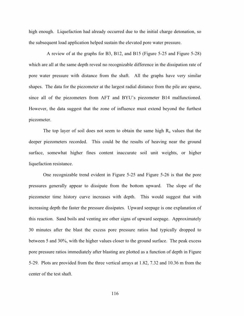
high enough. Liquefaction had already occurred due to the initial charge detonation, so

the subsequent load application helped sustain the elevated pore water pressure.

A review of at the graphs for B3, B12, and B15 (Figure 5-25 and Figure 5-28)

which are all at the same depth reveal no recognizable difference in the dissipation rate of

pore water pressure with distance from the shaft. All the graphs have very similar

shapes. The data for the piezometer at the largest radial distance from the pile are sparse,

since all of the piezometers from AFT and BYU’s piezometer B14 malfunctioned.

However, the data suggest that the zone of influence must extend beyond the furthest

piezometer.

The top layer of soil does not seem to obtain the same high Ru values that the

deeper piezometers recorded. This could be the results of heaving near the ground

surface, somewhat higher fines content inaccurate soil unit weights, or higher

liquefaction resistance.

One recognizable trend evident in Figure 5-25 and Figure 5-26 is that the pore

pressures generally appear to dissipate from the bottom upward. The slope of the

piezometer time history curve increases with depth. This would suggest that with

increasing depth the faster the pressure dissipates. Upward seepage is one explanation of

this reaction. Sand boils and venting are other signs of upward seepage. Approximately

30 minutes after the blast the excess pore pressure ratios had typically dropped to

between 5 and 30%, with the higher values closer to the ground surface. The peak excess

pore pressure ratios immediately after blasting are plotted as a function of depth in Figure

5-29. Plots are provided from the three vertical arrays at 1.82, 7.32 and 10.36 m from the

center of the test shaft.

116

The peak excess pore pressure ratios at this time are typically between 80 and

100% with the lowest values at the top of the profile. Similar plots are provided in Figure

5-30 to show the peak excess pore pressure ratio versus depth during the first statnamic

load test. Peak excess pore pressure ratios are typically between 70 and 100% which is

somewhat lower than that immediately after blasting as a result of pore pressure

dissipation. It took about 3 minutes to reduce the lowest piezometer reading to 10%.

117

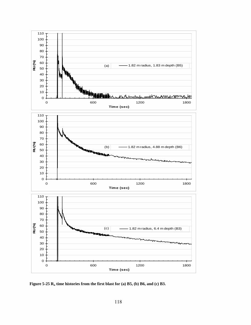
0

10

20

30

40

50

60

70

80

90

100

110

0 600 1200 1800Time (sec)

RU

(%)

1.82 m radius, 1.83 m depth (B5)(a)

0

10

20

30

40

50

60

70

80

90

100

110

0 600 1200 1800Time (sec)

RU

(%)

1.82 m radius, 4.88 m depth (B6)(b)

0

10

20

30

40

50

60

70

80

90

100

110

0 600 1200 1800Time (sec)

RU

(%)

1.82 m radius, 6.4 m depth (B3)(c)

Figure 5-25 Ru time histories from the first blast for (a) B5, (b) B6, and (c) B3.

118

0

10

20

30

40

50

60

70

80

90

100

110

0 600 1200 1800Time (sec)

RU

(%)


0

10

20

30

40

50

60

70

80

90

100

110

0 600 1200 1800Time (sec)

RU

(%)


0

10

20

30

40

50

60

70

80

90

100

110

0 600 1200 1800Time (sec)

RU

(%)



119

0

10

20

30

40

50

60

70

80

90

100

110

0 600 1200 1800Time (sec)

RU

(%)


0

10

20

30

40

50

60

70

80

90

100

110

0 600 1200 1800Time (sec)

RU

(%)


0

10

20

30

40

50

60

70

80

90

100

110

0 600 1200 1800Time (sec)

RU

(%)



120

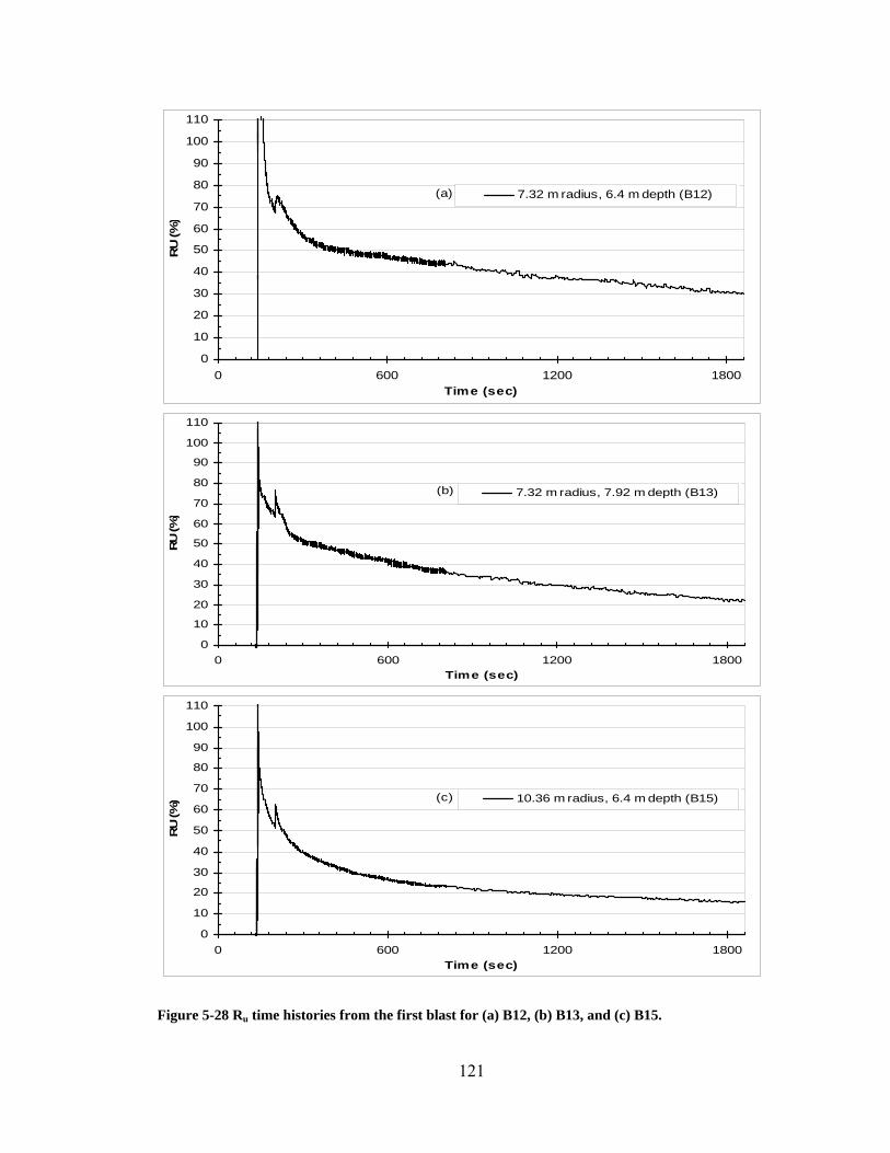
0

10

20

30

40

50

60

70

80

90

100

110

0 600 1200 1800Time (sec)

RU

(%)


0

10

20

30

40

50

60

70

80

90

100

110

0 600 1200 1800Time (sec)

RU

(%)


0

10

20

30

40

50

60

70

80

90

100

110

0 600 1200 1800Time (sec)

RU

(%) 10.36 m radius, 6.4 m depth (B15)(c)


121

0

2

4

6

8

10

12

14

0 20 40 60 80 100 120Ru (%)

Dep

th (m

)

Inner Ring(1.83 m)

Middle Ring(7.3 m)

Outer Ring(10.36 m)

Figure 5-29 Peak Ru versus depth plots for the first load test immediately after the charges were detonated.

122

0

2

4

6

8

10

12

0 20 40 60 80 100 12

Pore Pressure (%)

Dept

h (m

)

0

inner ringmiddle ringouter ring

Figure 5-30 Peak Ru versus depth for the first load test just after the statnamic device was fired.

5.4.2 Second Blast Piezometer Readings

Figure 5-31 through Figure 5-34 plot the time histories of the excess pore water

pressure ratios (Ru) at the locations of the piezometers that functioned during the second

blast test. The radial distance and the depths of the piezometers indicated on each of the

plots. Once again the plots are organized according to radial distance from the pile, then

by depth below the ground surface.

The peak excess pore pressure ratios immediately after blasting are plotted as a

function of depth in Figure 5-35. Plots are provided from the three vertical arrays at 1.82,

123

7.32 and 10.36 m from the center of the test shaft. The peak excess pore pressure ratios

at this time are typically between 80 and 100% with the lowest values at the top of the

profile. Similar plots are provided in Figure 5-36 to show the peak excess pore pressure

ratio versus depth during the second statnamic load test. Peak excess pore pressure ratios

are typically between 70 and 100% which is somewhat lower than that immediately after

blasting as a result of pore pressure dissipation.

In general the second blast achieved the same peak pore pressures as the first

blast. If there was a lower pore pressure it was only a few percent. The dissipation rates

seem to increase slightly with each consecutive test. The shortest amount of time it took

for the pressures to decrease to 10% was about 4.4 minutes for the second test. Again the

dissipation tended to start from the bottom layers and moved upwards.

124

0

10

20

30

40

50

60

70

80

90

100

110

10200 10800 11400 12000 12600 13200 13800 14400Time (sec)

RU (%

)


0

10

20

30

40

50

60

70

80

90

100

110

10200 10800 11400 12000 12600 13200 13800 14400Time (sec)

RU

(%)


0

10

20

30

40

50

60

70

80

90

100

110

10200 10800 11400 12000 12600 13200 13800 14400Time (sec)

RU

(%)


Figure 5-31 Ru time histories from the second blast for (a) B5, (b) B6, and (c) B3.

125

0

10

20

30

40

50

60

70

80

90

100

110

10200 10800 11400 12000 12600 13200 13800 14400Time (sec)

RU

(%)


0

10

20

30

40

50

60

70

80

90

100

110

10200 10800 11400 12000 12600 13200 13800 14400Time (sec)

RU

(%)


0

10

20

30

40

50

60

70

80

90

100

110

10200 10800 11400 12000 12600 13200 13800 14400Time (sec)

RU

(%)



126

0

10

20

30

40

50

60

70

80

90

100

110

10200 10800 11400 12000 12600 13200 13800 14400Time (sec)

RU

(%)


0

10

20

30

40

50

60

70

80

90

100

110

10200 10800 11400 12000 12600 13200 13800 14400Time (sec)

RU

(%)


0

10

20

30

40

50

60

70

80

90

100

110

10200 10800 11400 12000 12600 13200 13800 14400Time (sec)

RU

(%)



127

0

10

20

30

40

50

60

70

80

90

100

110

10200 10800 11400 12000 12600 13200 13800 14400Time (sec)

RU

(%)


0

10

20

30

40

50

60

70

80

90

100

110

10200 10800 11400 12000 12600 13200 13800 14400Time (sec)

RU

(%)


0

10

20

30

40

50

60

70

80

90

100

110

10200 10800 11400 12000 12600 13200 13800 14400Time (sec)

RU



128

0

2

4

6

8

10

12

14

0 20 40 60 80 100 120Ru (%)

Dep

th (m

)

Inner Ring(1.83 m)Middle Ring(7.3 m)Outer Ring(10.36 m)

Figure 5-35 Peak Ru versus depth plots for the second load test immediately after the charges were detonated.

129

0

2

4

6

8

10

12

0 20 40 60 80 100 120

Pore Pressure (%)D

epth

(m)


Figure 5-36 Peak Ru versus depth plots for the second load test immediately after the statnamic device was fired.

5.4.3 Third Blast Piezometer Readings

Figure 5-37 through Figure 5-40 plot the time histories of the excess pore water

pressures (Ru) at the location of the piezometers that functioned during the third test. The

radial distance from the center of the test shaft and the depth below ground surface of the

piezometers are indicated on each of the plots. The plots are organized according to

radial distance from the pile, then by depth below the ground surface.

The peak excess pore pressure ratios immediately after blasting are plotted as a

function of depth in Figure 5-41. Plots are provided from the three vertical arrays at 1.82,

130

7.32 and 10.36 m from the center of the test shaft. The peak excess pore pressure ratios

at this time are typically between 80 and 100% with the lowest values at the top of the

profile. Similar plots are provided in Figure 5-42 to show the peak excess pore pressure

ratio versus depth during the third statnamic load test. Peak excess pore pressure ratios

are typically between 70 and 100% which is somewhat lower than that immediately after

blasting as a result of pore pressure dissipation.

In general the third blast achieved the same peak pore pressures as the first and

second blasts. Some were slightly higher, and if there was a lower pore pressure it was

only a few percent. Again the dissipation rates increased slightly. The shortest amount

of time it took for the lowest piezometer pressure to decrease to 10% was about 9.7

minutes for the third test. Just like load test 1 and 2, the dissipation tended to start from

the bottom layers and moved upwards for load test 3.

131

0

10

20

30

40

50

60

70

80

90

100

110

14340 14940 15540 16140 16740 17340 17940 18540 19140Time (sec)

RU

(%)


0

10

20

30

40

50

60

70

80

90

100

110

14340 14940 15540 16140 16740 17340 17940 18540 19140Time (sec)

RU

(%)


0

10

20

30

40

50

60

70

80

90

100

110

14340 14940 15540 16140 16740 17340 17940 18540 19140Time (sec)

RU

(%)


Figure 5-37 Ru time histories from the third blast for (a) B5, (b) B6, and (c) B3.

132

0

10

20

30

40

50

60

70

80

90

100

110

14340 14940 15540 16140 16740 17340 17940 18540 19140Time (sec)

RU

(%)


0

10

20

30

40

50

60

70

80

90

100

110

14340 14940 15540 16140 16740 17340 17940 18540 19140Time (sec)

RU

(%)


0

10

20

30

40

50

60

70

80

90

100

110

14340 14940 15540 16140 16740 17340 17940 18540 19140Time (sec)

RU

(%)



133

0

10

20

30

40

50

60

70

80

90

100

110

14340 14940 15540 16140 16740 17340 17940 18540 19140Time (sec)

RU

(%)


0

10

20

30

40

50

60

70

80

90

100

110

14340 14940 15540 16140 16740 17340 17940 18540 19140Time (sec)

RU

(%)


0

10

20

30

40

50

60

70

80

90

100

110

14340 14940 15540 16140 16740 17340 17940 18540 19140Time (sec)

RU

(%)



134

0

10

20

30

40

50

60

70

80

90

100

110

14340 14940 15540 16140 16740 17340 17940 18540 19140Time (sec)

RU

(%)


0

10

20

30

40

50

60

70

80

90

100

110

14340 14940 15540 16140 16740 17340 17940 18540 19140Time (sec)

RU

(%)


0

10

20

30

40

50

60

70

80

90

100

110

14340 14940 15540 16140 16740 17340 17940 18540 19140Time (sec)

RU



135

0

2

4

6

8

10

12

14

0 20 40 60 80 100 120Ru (%)

Dep

th (m

)

Inner Ring(1.83 m)Middle Ring(7.3 m)Outer Ring(10.36 m)

Figure 5-41 Peak Ru versus depth plots for the third load test immediately after the charges were detonated.

136

0

2

4

6

8

10

12

0 20 40 60 80 100 12

Pore Pressure (%)

Dept

h (m

)

0


Figure 5-42 Peak Ru versus depth plots for the third load test immediately after the statnamic device was fired.

5.5 Comparison of the Three Load Test Results

To provide a better representation of what is happening during all three tests, a set

of graphs have been prepared to compare the three tests. In Figure 5-43, all three of the

total pile head load versus deflection graphs has been plotted together. As mentioned

previously, the load and, hence, deflection increase from one test to the next can readily

be seen in these graphs. As noted previously, there is some residual deflection (about

137

5 mm) at the start of the second test. Despite the larger deflection for the second test, the

residual deflection at the beginning of the third test is still about the same as at the start of

the second test. A review of the curves of Figure 5-43 indicates that the loading stiffness

of the test shaft increases with each test despite the fact that the soil is being reloaded and

might be expected to weaken. This could result from either densification after each blast

or due to increased damping resistance owing to the progressively increasing velocity

during loading.

The area within each loading loop for each test represents the amount of energy

lost in one loading and unloading cycle due to damping. Comparing the static load-

deflection graphs of MP-1 (see Figure 2-10) to those of MP-3, the area of the hysteretic

loop is much larger as would be expected for a dynamic test. In a static test, the

movement is supposed to be slow enough to avoid both inertial and damping forces.

For all three tests, the rise time, (or the time it takes to reach peak load) are all

almost exactly the same for all three test. From examining the load and deflection time

histories for the three tests, one would notice that the peak load is achieved before the

peak deflection. This results in a lag time. The lag times for all three tests were similar

also. This would suggest that the soil did not contribute a great deal in the lag time. The

enormity of the pile creates a large inertial force that slows the reaction time. If the soil

contributed to the lag time, one would expect the first test to have the largest lag time and

get progressively smaller for each test since the change in deflection decreases with each

test as shown in Figure 5-43. Table 5-1 compares the rise time, lag time, peak

accelerations, and peak velocities for all three tests.

138

-1000

0

1000

2000

3000

4000

5000

6000

7000

-20 0 20 40 60 80

Deflection (mm)

Load

(kN

)

100

Load Test 3Load Test 2Load Test 1

Figure 5-43 Comparison of the three applied pile head load versus deflection curves.

Table 5-1 Comparison of rise time, lag time, peak acceleration, and peak velocity.

Rise Time

(s)

Lag Time (s)

Peak Deflection

(mm)

Peak Load (kN)

Peak Acceleration

(g)

Peak Velocity

(m/s) Test 1 0.14 0.065 59.6 4506 -3.59 0.98 Test 2 0.13 0.071 87.4 5497 -4.21 1.30 Test 3 0.13 0.071 98 6578 -4.88 1.55

Figure 5-44 compares the maximum positive and negative baseline corrected

accelerations, velocities, and deflections as a function of depth for all three tests. As the

load increased, the peak accelerations, velocities and deflection all increased as expected.

Peak positive accelerations at the pile head range from 2.4 to 3.2 g, while peak negative

accelerations are between 3.6 and 5 g. The peak negative accelerations in lateral

statnamic tests are typically larger in magnitude than the peak positive values. During

loading, the positive acceleration is reduced because the soil in front of the pile restricts

motion. Negative acceleration is aided by the soil pressure in front of the pile, as well as

reduced pressure behind the pile due to gapping. Peak accelerations decrease fairly

139

linearly with depth and are only 0.4 to 0.8 g at a depth of 15 m below ground where the

last accelerometer was located. The acceleration levels produced by the statnamic tests

are substantially higher than might be expected for large magnitude earthquake events

(0.3 to 1.5 g).

The peak positive velocities range from about 0.9 to 1.5 m/sec at the pile head.

Peak velocities from strong ground motion in a large earthquake would typically be about

1 m/sec/g. Therefore, these peak velocities would correspond to a large magnitude

earthquake with peak acceleration values ranging from 0.9 to 1.5 g. Because the velocity

levels correspond to those produced by earthquakes and because damping is proportional

to velocity, the observed damping behavior is likely representative of that for a prototype

pile subjected to strong ground shaking. Despite the higher peak negative acceleration

levels, the peak positive velocities are all higher than the peak negative velocities as are

the deflections.

Although the peak positive pile head deflections are 60 to 95 mm, the peak

negative deflections are only 10 to 20 mm. These positive deflection levels are on the

order of what might be acceptable for a large pile foundation for a bridge. The

deflections decrease rapidly with depth below the load point. Based on a third-order

polynomial fit to the deflection versus depth curve, the “effective length” of the pile

which is moving during the lateral test has been estimate to be approximately 16.12 m. A

better explanation of the process used to develop the effective length is provided in

Section 6.3.1

Figure 5-45 provides plots of the excess pore pressure ratio time histories for one

piezometer during the three lateral load tests. The piezometer is located on the outer ring

140

at a depth of 6.4 m below the ground surface. If the graphs for all three tests are

compared and put on the same graph, there are very slight differences in the peak

piezometer reading for the three load tests. The similarity of the graphs shows that

repeated liquefaction can be obtained within a test environment. Table 5-2 through Table

5-4 present the Ru values immediately after the detonation of the charges, before the

statnamic device has been fired, and after the statnamic loading is over, for tests 1

through 3, respectively. Contour plots were made for all three tests to provide a visual

representation of Ru within the soil profile after the down-hole charges were detonated

and after the statnamic loading. These contour plots are presented in Figure 5-46 through

Figure 5-51.

141

-3.0

-1.0 1.0 3.0 5.0 7.0 9.0 11.0

13.0

15.0

17.0-8.

0-6.

0-4.

0-2.

00.0

2.04.0

Max.

Acce

lerati

on (g

's)

Depth Below Ground (m)

Test

3 Pos

.

Test

3 Neg

.

Test

2 Pos

.

Test

2 Neg

.

Test

1 Pos

.

Test

1 Neg

.

-3.0

-1.0 1.0 3.0 5.0 7.0 9.0 11.0

13.0

15.0

17.0-1.

00.0

1.02.0

Max.

Veloc

ities (

m/s)

Depth Below Ground (m)Te

st 3 P

os.

Test

3 Neg

.

Test

2 Pos

.

Test

2 Neg

.

Test

1 Pos

.

Test

1 Neg

.

-3.0

-1.0 1.0 3.0 5.0 7.0 9.0 11.0

13.0

15.0

17.0

-50

050

100

150

Max.

Defle

ction

(mm

)

Depth Below Ground (m)

Test

2 Pos

.

Test

3 Neg

.

Test

2 Pos

.

Test

2 Neg

.

Test

1 Pos

.

Test

1 Neg

.

Figure 5-44 Maximum positive and negative acceleration, velocity, and deflection for all three tests.

142

0

10

20

30

40

50

60

70

80

90

100

110

0 600Time (sec)

RU

(%)

10.36 m radius, 6.4 m depth (B15) Test 110.36 m radius, 6.4 m depth (B15) Test 210.36 m radius, 6.4 m depth (B15) Test 3

Figure 5-45 Comparison of the piezometer readings for the three tests.

Table 5-2 Ru values after detonation, before and after loading for load test 1.

BLAST 1

Depth Below

Ground (m) Piezometer

After Blast (%)

Before Statnamic (%)

After Statnamic (%)

1.8 B5 74.0 50.8 48.9 3.2 B4 79.7 80.7 79.7 4.9 B6 98.0 75.9 84.3 6.4 B3 97.3 77.4 86.7 7.9 B7 88.1 73.4 80.5 10.7 B2 80.5 65.8 74.1 11 B8 88.3 72.4 82.0

Inner Ring

11.9 B1 90.1 63.8 82.5 1.8 B11 76.5 43 59.1 3.4 B10 110.9 96.9 104.1 6.4 B12 191.6 68.0 69.7

Middle Ring

7.9 B13 86.4 66.2 74.3 Outer Ring 6.4 B15 88.9 54.2 62.1

143


BLAST 2

Depth Below


After Blast (%)


After Statnamic (%)

1.8 B5 81.7 75.9 87.5 3.2 B4 33.5 35.4 35.9 4.9 B6 100.4 83.7 87.6 6.4 B3 91.1 81.5 87.9 7.9 B7 81.0 71.2 80.5 10.7 B2 77.7 68.8 74.8 11 B8 85.7 79.0 84.5

Inner Ring

11.9 B1 88.0 74.7 85.6 1.8 B11 74.5 52.5 59.1 3.4 B10 109.8 93.5 97.3 6.4 B12 76.6 83.3 84.6

Middle Ring

7.9 B13 81.4 68.6 77.8 Outer Ring 6.4 B15 77.4 58.8 66.8


BLAST 3

Depth Below


After Blast (%)


After Statnamic (%)

1.8 B5 74.0 98.0 62.4 3.2 B4 47.7 48.4 46.5 4.9 B6 102.0 89.5 92.4 6.4 B3 89.8 82.8 87.9 7.9 B7 79.5 71.8 77.9 10.7 B2 73.9 67.6 69.5 11 B8 85.7 77.3 83.1

Inner Ring

11.9 B1 86.7 74.3 84.9 1.8 B11 78.4 64.1 74.5 3.4 B10 101.9 85.1 97.3 6.4 B12 161.8 120.2 121.3

Middle Ring

7.9 B13 72.2 60.4 67.2 Outer Ring 6.4 B15 73.3 55.4 63.7

144

Figure 5-46 Excess pore pressure ratio contours (in percent) for the soil profile mass immediately after the detonation of the charges for test 1.

Figure 5-47 Excess pore pressure ratio contours ( in percent) for the soil mass immediately after the statnamic loading for test 1.

145

Figure 5-48 Excess pore pressure ratio contours (in percent) for the soil mass immediately after the detonation of the charges for test 2.

Figure 5-49 Excess pore pressure ratio contours (in percent) for the soil mass immediately after the statnamic loading for test 2.

146

Figure 5-50 Excess pore pressure ratio contours (in percent) for the soil mass immediately after the detonation of the charges for test 3.

Figure 5-51 Excess pore pressure ratio contours (in percent) for the soil mass immediately after the statnamic loading for test 3.

147

6 Analysis

6.1 Introduction

There are several ways to evaluate lateral load-deflection relationships for deep

foundations. This chapter will discuss two of these methods. The first approach is the

derivation of p-y curves directly from strain data as described in Figure 1-1 and involves

the following steps:

1. Calculate curvature at each strain gauge depth using the strain data.

2. Derive deflection versus depth profile from curvatures through double

integration.

3. Develop moment versus depth plots.

4. Estimate soil pressure from moments through double differentiation.

5. Construct p-y curves for each station from the derived pressures and deflections.

The second approach to validating p-y curves is by direct empirical evaluation

based on a comparison of measured and computed response. In this approach, various

assumptions regarding p-y curve shapes are used in computing pile head load-deflection

relationships and then, computed response is compared with measured response. These

analyses have been performed using a soil-structure interaction program called LPILE 5

Plus, version 5m (2004). LPILE was produced by Ensoft Inc. which uses the finite

difference method. The assumed p-y curve which produces the best agreement with the

149

measured response is considered to be the best representation of the true lateral soil

resistance. Each of these approaches has been used during this study and the following

sections detail the results obtained from each procedure.

6.2 Calculating P-Y Curves from Strain Data

6.2.1 Calculating Curvature from Strain

During the construction of the pile, strain gauges were attached to the rebar cage,

as described in Chapter 4. For the first five stations below the ground surface, there were

only strain gauges in line with the direction of loading, but for the last five stations strain

gauges were installed perpendicular to the direction of loading. The strain gauges in the

direction of loading are used to calculate the curvature of the shaft with depth. The

curvature (κ) was computed using the equation

dct εε

κ−

= (6-1)

where, εt is the measured tensile strain, εc is the measured compressive strain, and d is the

distance between gauges which was 2.14 m in this case.

Analysis of the strain data reveals that most of the strain in the shaft seemed to

occur at or near the top of the Cooper Marl. At low deflection levels, all of the strain

gauges seemed to function as expected, and the strain profiles had reasonable shapes.

However, as deflections increased, the recorded strain appeared to be excessive because

the integrated curvature profile produced a deflection at the top of the shaft which was

greater than that which was actually measured. A definite reason for this occurrence

could not be determined; however, it is believed that cracking contributed to the

150

excessive curvature observed. The tensile strains did not maintain proportionality with

the compressive strains. The compression side of the shaft did not crack, since concrete

is very strong in compression. Being able to use strains from the compression side of the

shaft only might have solved the problem of excessive strain due to cracking.

Solving curvature from strain with one strain gauge can be done, but it is difficult.

In linearly elastic, homogeneous material it is much simpler, because the neutral axis

doesn’t shift from the center as long as the material is not loaded past its elastic limit. In

a non-homogeneous pile with nonlinear materials, the same is not true. As the pile is

loaded past the tensile strength of concrete, for example, the neutral axis shifts. It is

difficult to track where the neutral axis is within a pile at every moment in time, which is

why it is so difficult to solve for the curvature with one strain gauge. The equation for

curvature with one strain gauge changes to

ndεκ = (6-2)

where κ is the curvature, ε is the strain for the desired side, and dn is the distance from the

strain gauge to the neutral axis.

The computer programs LPILE and Xtract (the latter developed by Xtract, 2004)

were used to track where the neutral axis theoretically should be during the testing of

MP-3 by using various nonlinear models. Unfortunately, these attempts to compute

curvature vased only on the compression strain gauge proved inadequate with the

computed deflections still being excessive. If the non-linear model along with the strains

was correct, the neutral axis should have been outside the pile in some cases. In other

words, the pile was cracked all the way through and the whole pile was in tension. This

is unrealistic, given the loads used and the size of the pile. Nevertheless, the process of

151

solving for p-y curves from strains was continued to see what the result would be. The

following figures show the progression of curvature through time with respect to depth

using Equation 6-1. No adjustments were made for the changing stiffness of the shaft.

0

5

10

15

20

25

30

-200 0 200 400 600 800 1000

Curvature (1/m)

Dep

th (m

)

0.5 s0.55 s

0.575 s

0.6 s0.625 s

0.65 s

0.85 s0.89 s

Figure 6-1 Time step curvatures calculated from strain gauges for test 1 of MP-3.

152

0

5

10

15

20

25

30

-600 -400 -200 0 200 400 600 800 1000 1200

Curvature (1/m)

Dep

th (m

)

0.5 s

0.55 s

0.575 s

0.6 s

0.625 s

0.65 s

0.85 s

0.89 s


153

0

5

10

15

20

25

30

-600 -400 -200 0 200 400 600 800 1000 1200

Curvature (1/m)D

epth

(m)

0.5 s

0.55 s

0.575 s

0.6 s

0.625 s

0.65 s

0.85 s

0.89 s


6.2.2 Derivation of Deflection Profile from Curvature

The deflections with depth were derived to check if they matched the acceleration

derived deflections. If the deflections match those of the accelerations, we know the

strain data are reliable since the acceleration derived deflections have matched reasonably

well with the LVDT-based pile head deflections.

154

The first step in calculating the deflections with depth profile is to make a few

boundary condition assumptions. Assuming the pile could be modeled like a cantilever

beam, the point of fixity would then be at 30 m below the ground. This depth was chosen

because the strains at the deepest strain gauge are very small and this point is another

couple of meters below that. The slope and curvature at 30 m are also assumed to be

zero. A free-head condition was also assumed based on the fact that the hemispherical

bearing was used. In other words, the load applied at the top does not apply a moment.

After computing the deflections from strain, the computed deflection was

somewhat high when compared to the deflections from both the LVDT pile-head

deflection and the acceleration derived deflections. As indicated previously, one likely

explanation for the overestimation of the deflection would be excessive strain on the

tension side of the pile which could be explained by cracking within the concrete portion

of the pile.

6.2.3 Development of Moment versus Depth Plots

Solving for the moments in a prismatic beam with linearly elastic material that

follows Hooke’s law is quite simple if the curvatures are already calculated. The

equation for moment is:

EIM κ= (6-3)

where M is the bending moment of the beam or pile, EI is the flexural rigidity or

stiffness, and κ is the curvature. This equation shows the simplicity of calculating the

moment when the criteria are met as described previously. However, test shaft MP-3 is

not linearly elastic, and there are section property changes with depth. These

characteristics make the analysis more complicated.

155

As mentioned in Chapter 4, MP-3 is composed of two different cross-sections.

The first section is the portion of the pile where the steel casing covers the concrete and

the second is the remaining portion of the pile without the steel casing. An elevation

view of this can be seen in Figure 4-43.

The most difficult part of calculating moments is finding the flexural stiffness (EI)

of the pile. Three parts of the first cross-section contribute to the stiffness: steel casing,

steel reinforcement, and the concrete. The moment of inertia can be calculated based

purely on the geometry shown in Figure 4-43, resulting in the following:

• Icasing = 0.1684 m4

• Ireinforcement = 0.0532 m4

• Iconcrete(uncracked) = 1.990 m4

A yield strength of 414 MPa (60 ksi) and a typical modulus of elasticity of 200 GPa

(29,000 ksi) were assumed for the reinforcement. The steel casing was composed of 248

MPa (36 ksi) steel with the same modulus of elasticity as the reinforcement. The

modulus of elasticity for the concrete was calculated using a common empirical formula

for normal weight concrete based on the 28-day compressive strength.

'000,733,4 cconcrete fE = (6-4)

where Econcrete is the modulus of elasticity of concrete with units of Pa and fc’ is the

average 28-day compressive strength of the concrete with units of N/m2. Based on six

compression tests at the time of testing, the average concrete compression strength was

42.7 MPa, which leads to a Young’s Modulus for the concrete of 30.9 GPa according to

Equation 6-4.

156

Ideally, another strain gauge placed at the ground surface would have helped take

some of the uncertainty out of determining the flexural stiffness of the shaft. The

moments at this location could have been calculated, by multiplying the applied load by

the height of the shaft above the ground surface. Using this computed moment and the

measured strain, the stiffness of the shaft could have been determined. Unfortunately,

there was no strain gauge at the ground surface, so the stiffness of the shaft was based on

the empirical Equation 6-4 and the stiffness calculated by Hales (2003) for MP-1, which

was built to the same specifications as MP-3.

Cracking increases the complexity of calculating the flexural stiffness of the shaft.

As soon as the shaft is loaded past the tensile strength of concrete, the section cracks up

to the neutral axis, decreasing its stiffness. It is very difficult to determine this change in

stiffness, and the rate of loading only added to the difficulty. The curvature and the

amount of cracking appear to vary non-uniformly at each strain gauge. These variations

can be seen in the curvature time-step graphs in Figure 6-1 through Figure 6-3. Since the

cracking was not a sudden discrete break, it was difficult to model the change in stiffness.

An Excel® spreadsheet named PY_BY_U was used to calculate both the moment

(discussed in this section) and soil pressure (discussed in the next section). This

spreadsheet developed by Dr. Travis Gerber while working on his dissertation was

modified to compensate for the non-linear behavior of MP-3. A linear piece-wise

function was used to model the change in stiffness due to cracking. However, as was

with the determination of curvature, completely satisfactory bending moment profile

could not be obtained.

157

6.2.4 Estimating Soil Pressure from Moments

Despite having questionable bending moment and curvature profiles, additional

analyses were undertaken to calculate soil pressures and see what p-y curves resulted. To

estimate the soil pressures from moments the spreadsheet mentioned in the previous

section was employed.

While conceptually simple, obtaining soil pressures from double differentiation of

bending moments is not straight forward. The approach employed by the spreadsheet

involves differentiation of successive sets of fitted cubic polynomials. Additional details

regarding the process are described in Gerber (2003).

6.2.5 Constructing P-Y Curves

PY_BY_U produces an output file containing the soil pressures and deflections

for each strain gauge station. These values were plotted to produce p-y curves.

Unfortunately the p-y curves proved to be unrealistic. One significant factor contributing

to the unrealistic shapes was the extreme discontinuity in curvature and moment at the

Cooper Marl interface. The extreme discontinuity in moment coupled with the relative

large spacing between strain gauges prevented a good fit of cubic polynomials to the

moment data. In trying to fit the cubic polynomial, some of the pressures came out to be

negative, which is virtually impossible. Negative pressures imply that the soil behind the

shaft was pushing it forward.

Another big contributor to the difficulty of calculating the soil pressures was the

lack of reliable strain data. After filtering out the stain gauges that malfunctioned, only

two strain gauges where left. To compensate for the removed stain gauges, interpolated

gauges based on the strains measured by the two remaining gauges were placed in the

158

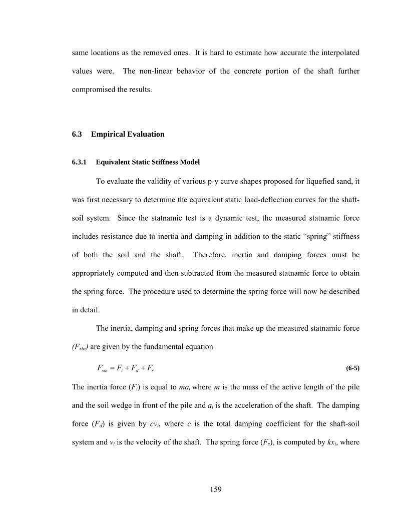
same locations as the removed ones. It is hard to estimate how accurate the interpolated

values were. The non-linear behavior of the concrete portion of the shaft further

compromised the results.

6.3 Empirical Evaluation

6.3.1 Equivalent Static Stiffness Model

To evaluate the validity of various p-y curve shapes proposed for liquefied sand, it

was first necessary to determine the equivalent static load-deflection curves for the shaft-

soil system. Since the statnamic test is a dynamic test, the measured statnamic force

includes resistance due to inertia and damping in addition to the static “spring” stiffness

of both the soil and the shaft. Therefore, inertia and damping forces must be

appropriately computed and then subtracted from the measured statnamic force to obtain

the spring force. The procedure used to determine the spring force will now be described

in detail.

The inertia, damping and spring forces that make up the measured statnamic force

(Fstn) are given by the fundamental equation

sdistn FFFF ++= (6-5)

The inertia force (Fi) is equal to mai where m is the mass of the active length of the pile

and the soil wedge in front of the pile and ai is the acceleration of the shaft. The damping

force (Fd) is given by cvi, where c is the total damping coefficient for the shaft-soil

system and vi is the velocity of the shaft. The spring force (Fs), is computed by kxi, where

159

k is the static stiffness constant of the shaft-soil system and xi is the deflection of the

shaft.

Previous studies for example, (Brown, 2000; and Rollins et al., 2005) have

analyzed lateral statnamic pile load tests by lumping the entire mass at the load point and

modeling the system using a single degree-of-freedom approach. However, the data from

the downhole accelerometers in this test make it possible to use a much more realistic

model of the shaft-soil system. In this study, the analysis was performed by treating the

shaft as a ten degree-of-freedom system with the location of each accelerometer as the

center of each lumped mass. This is still a simplification of a very complex system, but

should provide more accurate results than a single degree-of-freedom model.

Determination of Inertial Force

To calculate the total inertial force, the lumped masses were multiplied by the

measured acceleration data collected by the DMLSs and summed at each time step. The

mass of the system consisted of both the mass of the test shaft and the mass of the soils

moving during the test. The mass of the test shaft was relatively simple to calculate using

the shaft dimensions and the mass densities of the materials used in its construction.

Because only the upper section of the shaft was actually in motion during the statnamic

load test, only the mass of this “active” length was used in the calculations. Although a

number of theoretical expressions are available with which to compute the active length

for example (Gazetas and Dobry, 1984), in this case the active length of the pile was

found by fitting a cubic polynomial curve to the acceleration derived deflection profile

and using the y-intercept of the curve as the active length. Figure 6-5 shows the

polynomial curve through the measured deflection points along with the equation of the

160

curve for the third statnamic load test. Based on this approach, the active length was

found to be equal to 16.12 m below the ground surface for the third test. Similar analyses

suggest that this length is about the same for each test.

The mass of the soil moved during the test was estimated using the same cubic

polynomial curve developed to find the active length. The deflection versus depth profile

from the polynomial curve was integrated to find the minimum area of soil moved. This

area was then multiplied by the average width of the shear zone at each depth which was

assumed to shear at a 35o angle from the sides of the pile. From these dimensions the

minimum volume of soil moved during the test could be calculated. A typical density for

sand (19.64 kN/m3) was then used to calculate soil mass moving with the test shaft.

Using this approach the mass of the soil was found to be about 2% of the mass of the

shaft itself. A model of the lumped shaft and soil mass distribution along the length of

the shaft is presented in Figure 6-4, which shows the locations of the masses along with

the mass of the shaft at each level. A small beam was attached to the top of the test shaft

that was not taken into account in the mass calculations due to lack of information. If this

beam were included, this would increase the inertial force produced at the pile head by a

small amount.

161

Figure 6-4 Model used to calculate the inertial force (relative size of the masses provides an approximate indication of mass distribution).

162

y = -1E-05x3 + 0.0019x2 - 0.2742x + 16.117R2 = 0.9987

-3.0

-1.0

1.0

3.0

5.0

7.0

9.0

11.0

13.0

15.0

17.0

0 20 40 60 80 10Max. Deflection (mm)

Dep

th B

elow

Gro

und

(m)

0

Figure 6-5 Deflection profile for load test 3 used to find the active length.

Determination of Damping Force

Although the velocity of the pile was easily found by integrating acceleration, as

discussed in Section 5.3, the damping coefficient could only be constrained within a

range. Ultimately, the exact value had to be determined in a trial and error process. The

damping force can be expressed in terms of a dimensionless damping ratio (ζ) using the

equation

vcF cd ζ= (6-6)

where cc is the critical damping coefficient. The critical damping coefficient represents

the value for which the system will return to equilibrium after exactly one cycle.

163

The next step in the analysis is to calculate the natural frequency of the pile. This

can be done with the following equation

mc nc ω2= (6-7)

where wn is the natural frequency and m is the mass of the system. Because the damping

ratio in Equation 6-6 is dimensionless, it facilitates comparisons with other systems with

different mass and frequency values. Based on the measured deflection time history at the

load point, the damped natural period of vibration is between 0.40 to 0.45 seconds. The

undamped natural period will likely have a slightly higher range. Based on the measured

natural period, the natural frequency would be between 14 and 15.7 radians/s.

One challenging, but crucially important, part of the process is selecting an

appropriate damping ratio. An estimate of the damping ratio can be calculated by using

the log decrement method along with the measured deflection time history. The log

decrement is the rate at which the amplitude of a free vibration decreases with time in a

damped system (Rao, 2004). The log decrement (δ) is given by the equation

⎟⎟⎠

⎞⎜⎜⎝

⎛=

2

1

xxLNδ (6-8)

where x1 is the deflection at a particular time, and x2 is the deflection one cycle (or

period) away from x1. If the log decrement is calculated over multiple periods the

equation for the log decrement becomes

⎟⎟⎠

⎞⎜⎜⎝

⎛=

nxxLN

n11δ (6-9)

where n is the number of periods over which the log decrement is calculated as an

integer, x1 is a chosen deflection, and xn is the deflection of the nth cycle away from x1.

164

The log decrement can then be used to calculate the damping ratio (ζ) from the

measured response of the system using the equation

( ) 222 δπ

δζ+

= (6-10)

One criterion for the log decrement is that the system must be under free

vibration, in other words the load must be removed during vibration. For the statnamic

load test, the load in the system was not completely removed by the time the maximum

deflection occurred although it was relatively small. Therefore, there may be some error

in interpretation. For this reason the damping ratio was estimated using one and two

cycles to provide a range of possible values. The damping ratio computed using the log

decrement approach ranged from 30 to about 40%.

After estimating a damping ratio, the total damping force was computed for the

ten degree-of-freedom lumped mass system. At each mass in the system, the damping

force was computed using Equation 6-6, where the velocity was that derived from the

measured acceleration time history. The damping force was then weighted in proportion

to the fraction of the total mass of the shaft which the velocity represented. The total

damping force was then obtained by summing the damping force at each lumped mass for

each time step.

Determination of Spring Force

The final step in the analysis is to compute the spring force for the system. The

spring force can be determined using two different equations and, if appropriate

parameters are selected, the computed spring force should be the same. For example, the

spring stiffness can be computed from the mass and natural frequency using the equation

165

2nmwK = (6-11)

The spring stiffness is then multiplied by the deflection at any time to obtain the spring

force according to Equation 6-5.

The spring force can also be computed by rearranging Equation 6-5 to give the equation

distns FFFF −−= (6-12)

Therefore, after the damping force and the inertial force are calculated using the

procedures described previously, they can simply be subtracted from the statnamic force

applied to the test shaft as measured by the load cell to obtain the spring force (see

Equation 6-12).

The agreement between the spring force computed by Equation 6-11 and

Equation 6-12 is based on whether or not damping ratio, mass, and frequency of the shaft

were properly estimated. The various parameters can easily be iteratively adjusted within

acceptable ranges until the best agreement is obtained.

A plot of the static spring force-deflection curve obtained using Equation 6-11 is

presented along with the measured statnamic force-deflection curve for each statnamic

test firing in Figure 6-6 through Figure 6-8. The residual deflections at the beginning of

each test were added to the deflections calculated for a better comparison. In each test,

there is a substantial reduction in the stiffness of the force-deflection curve when

damping and inertia forces are subtracted and the force displacement loop becomes much

smaller. In addition, the spring force computed using the linear spring stiffness from

Equation 6-11 is shown in each figure (designated as “MP-3 Static Equivalent”) for

comparison purposes. In general, the linear spring force-deflection line from Equation

6-11 is in good agreement with loading portion of the force-deflection curve computed

166

using Equation 6-12 suggesting that the input parameters are reasonable. A summary of

the linear stiffness, natural period, and damping ratio assumed in calculating the curves in

Figure 6-6 through Figure 6-8 is provided in Table 6-1. A review of the data in Table 6-1

indicates that the values for natural period and damping ratio are well within the ranges

obtained from the measured deflection time histories discussed previously.

Figure 6-9 through Figure 6-11 provide plots of the measured statnamic force

time history along with the computed inertia, damping and spring force time histories for

each statnamic test firing. A review of the time histories suggest that the inertial force is

generally the major component of the increased dynamic lateral resistance observed

during a statnamic test. Although there are some time intervals where damping forces are

substantial, they generally accounted for 23% or less of the measured peak statnamic

force in these tests.

A summary plot showing the computed force-deflection loops for all three

statnamic tests is provided in Figure 6-12 for comparison purposes. This graph shows a

slight degradation of stiffness with subsequent loading. The decrease is greater between

the first and second load test than it is between the second and third load tests. There is

not a lot of evidence of gapping between the second and third test. The noise in the

accelerations from the first test makes seeing a gap between the first and second test more

difficult.

167

-2000

-1000

0

1000

2000

3000

4000

5000

6000

-15 0 15 30 45 60

Deflection (mm)

Load

(kN

)MP-3 Static EquivalentP-Multiplier-8BrownP-Multiplier-9No Resistance

Figure 6-6 Comparison of load-deflection curves for test 1.

-1000

0

1000

2000

3000

4000

5000

-15 0 15 30 45 60 75 90 105Deflection (mm)

Load

(kN)

MP-3 Static EquivalentP-Multiplier-8Brow nP-Multiplier-9No Resistance

Figure 6-7 Comparison of load-deflection curves for test 2.

168

-1000

0

1000

2000

3000

4000

5000

6000

-15 0 15 30 45 60 75 90 105

Deflection (mm)

Load

(kN)

MP-3 Static Equivalent

P-Multiplier-8Brow n

P-Multiplier-9No Resistance

Figure 6-8 Comparison of load-deflection curves for test 3

Table 6-1 Linear stiffness, natural period, and damping ratio used for each test.

Test 1 Test 2 Test 3 Linear Stiffness (kN/m) 58208 52544 52950

Natural Period (s) 0.42 0.44 0.44 Damping Ratio (%) 35 30 30

-3000

-2000

-1000

0

1000

2000

3000

4000

5000

0 0.2 0.4 0.6 0.8 1 1.2 1.4

Time (s)

Load

(kN)

Statnam ic LoadDam ping ForceInertial Force Spring Force

Figure 6-9 Plots of the measured statnamic force time history, computed inertia, damping and spring force time histories for test 1.

169

-5000

-3000

-1000

1000

3000

5000

0 0.2 0.4 0.6 0.8 1 1.2 1.4

Time (s)

Load

(kN)



-5000

-3000

-1000

1000

3000

5000

7000

0 0.2 0.4 0.6 0.8 1 1.2 1.4

Time (s)

Load

(kN

)



170

-2000

-1000

0

1000

2000

3000

4000

5000

-10 0 10 20 30 40 50 60 70 80 90 100

Time (s)

Load

(kN

)

Test 1Test 2Test 3

Figure 6-12 Comparison of the static equivalent load-deflection curves for all three tests.

6.3.2 Comparison with Other Studies

As noted previously, Brown (2000) used a single degree-of-freedom system to

model the soil-shaft interaction. The inertial force was calculated assuming the shaft

would act like a cylinder rotating around its base. By taking the mass moment of inertia

and multiplying it by the rotational acceleration at the pile head, the inertial force was

determined. The damping force was apparently calculated by increasing the damping

ratio until the force-deflection curve became a straight line, although little information is

provided on how this computation was actually performed. Damping ratios of 30%, 46%

and 46% were obtained for the three tests respectively. These values are similar to those

obtained in this study for the first test but are somewhat higher for the second and third

tests. An assumed stiffness which decayed logarithmically from a high initial value to a

constant lower value was used to simulate soil non-linearity. The resulting load-

171

deflection curves are relatively linear and are plotted for all three load tests along with the

load-deflection curves computed in this study in Figure 6-6 through Figure 6-8 The

stiffness used by Brown (2000) appears to be more of a secant stiffness drawn from the

origin to the peak deflection and is about 36% softer than the loading portion of the curve

for the first load test and 30% for the second and third load tests obtained in this study.

Comparison of MP-1 versus MP-3 Static Equivalent Stiffness

Figure 2-10 provides plots of the load-deflection curves for load tests performed

statically on shaft MP-1. The stiffest load-deflection curve is for conditions before blast

induced liquefaction. Two sets of curves are also provided in this figure for two tests

following blast induced liquefaction. The load-deflection curves soften considerably

after blasting and are quite similar for each test after accounting for the residual

deflections from the end of the first test. Despite the high speed pump unit, the hydraulic

actuators took over a minute to apply the load after the blast event. This allowed excess

pore water pressures to dissipate throughout the duration of the entire test. Inevitably, the

excess pore pressures for the static tests were smaller than those for shaft MP-3. A graph

of the peak pore pressures just after the first and second blasts during the testing on shaft

MP-1 are shown in Figure 2-11 and Figure 2-12. Comparing these figures with Figure

5-29, Figure 5-35, and Figure 5-41, slightly lower pore pressure ratios can be seen during

the tests performed on MP-1. Figure 6-13 compares the average excess pore pressure

ratio produced during testing for shafts MP-1 and MP-3.

A comparison between the static load-deflection curve for shaft MP-1 and the

equivalent static load-deflection curve from the second statnamic test on shaft MP-3 can

be seen in Figure 6-14 and Figure 6-15. The slopes of the load-deflection curves, after

172

both blasts, seem to be very close to the slope of the equivalent static stiffness calculated

for MP-3. This result tends to confirm the reliability of the procedure used to compute

the equivalent static load-deflection curve and the damping ratio which was selected. It

also indicates that the static load-deflection curve does have a loop rather than being a

single straight line. The second blast load-deflection curve for MP-1 start with residual

displacement, and that is why they do not match as well as the first load test. If the

residual deflection is removed, the slopes match as well as they do for the first blast.

0

2

4

6

8

10

12

14

30 50 70 90 110Excess Pore Pressure Ratio (%)

Dep

th (m

)

MP-1-First Blast & Cycle

MP-1-Second Blast- First Cycle

Avg. MP-3-Inner RingAvg. MP-3-Middle Ring

Avg. MP-3-Outer Ring

Figure 6-13 Average pore water pressures for the first blast, first cycle and the second blast, first cycle compared to the average pore pressures of all three load tests of MP-3.

173

-2000

-1000

0

1000

2000

3000

4000

5000

-20 0 20 40 60 80 100 120 140

Deflection (mm)

Load

(kN)


Spring Force

MP-1 First Blast

Figure 6-14 Comparison of the load deflection curve of the first blast of MP-1 and the static equivalent load deflection curve of MP-3.

-2000

-1000

0

1000

2000

3000

4000

5000

-20 0 20 40 60 80 100 120 140

Deflection (mm)

Load

(kN)


Spring Force

MP-1 Second Blast

Figure 6-15 Comparison of the load deflection curve of the second blast of MP-1 and the static equivalent load deflection curve of MP-3.

174

6.3.3 LPILE Derived P-Y Curves

As indicated previously in Chapter 2, several methods have been proposed for

defining p-y curves in liquefied sand. In this section, some of these approaches will be

used to model the liquefied sand, and the pile-head load-deflection curve will be

computed using the computer program LPILE Plus version 5.0.12. LPILE is a relatively

well-documented and useful program that calculates the lateral load response of deep

foundations based on user inputs of pile properties, soil layering and soil properties. The

load-displacement response of the shaft computed using LPILE will then be compared

with the equivalent static load-deflection curves developed in the previous section from

the Statnamic testing. The p-y curves for liquefied sand will include those proposed by

Rollins et al. (2005), Liu and Dobry (1995); Wilson (1998) and Wang and Reese (1998).

Additional, analyses will be performed assuming that the liquefied sand has no resistance

at all.

In all cases, the non-linear reinforced concrete model in LPILE was used to assess

the moment-curvature relationship for the test shaft. The material properties for the test

shaft were those defined in Chapter 4.

P-Y Curves for Liquefied Sand Proposed by Rollins et al. (2005)

Four soil layers were used to represent the subsurface materials in this model (see

Table 6-2). The first was a layer of sand that extended from the ground surface to a depth

of 1.5 m with the p-y curve defined using the API criteria (O’Neill and Murchison, 1983).

The water table at the Mt. Pleasant site fluctuated from the ground surface down to

approximately 1.5 m. In the analysis, the water table was assumed to be at around 1.5 m.

The unit weight of the first layer was taken as 19.5 kN/m3, φ (friction angle) as 38o, and k

175

(p-y modulus) as 58469 kN/m3 (215.4 pci) based on API sand criteria. The second layer

was also non-liquefiable and consisted of a soft clay that started at a depth of 1.5 m and

extended to 3.5 m. This layer was modeled using the soft clay curve developed by

Matlock (1970) with the buoyant unit weight as 10 kN/m3, c (undrained cohesion)

increasingly linearly from 25 kN/m2 at the top of the layer to 50 kN/m2 at the bottom of

the layer, and an ε50 (strain factor) of 0.02 which is typical for soft clay.

The third layer was liquefied sand which extended from a depth of 3.5 m to the

top of the Cooper Marl at 12.5 m. The p-y curve in this layer was modeled using the

concave upward shape proposed by Rollins et al., (2005) for layers where the relative

density was approximately 50%. However, based on the CPT profiles, there is a layer of

looser sand with a relative density of only 35 to 40% between 7 and 10.5 m below the

ground surface. Based on recommendations by Rollins et al., (2005) the p-y curve for

this layer has been assumed to be essentially flat. Therefore, a p-multiplier of 0.05 was

used for this layer to essentially eliminate any resistance. The buoyant unit weight for the

liquefied sand was set at 9.5 kN/m3.

Because the p-y curves for liquefied sand developed at Treasure Island were

based on a 0.324 m diameter pile, a p-multiplier is necessary to account for the much

larger test shaft diameter at this site. Based on analyses of the static blast liquefaction

tests, Hales (2003) recommended a p-multiplier of 8.0 to account for diameter effects.

Rollins et al., (2005) recommend a somewhat higher p-multiplier of 9.0. Therefore,

separate analyses were performed using both of these p-multiplier values.

The last layer, the Cooper Marl was modeled using a stiff clay with free water p-y

curve proposed by Reese et al., 1975. Based on available test data provided by Brown

176

and Camp (2002), the buoyant unit weight was taken as 10 kN/m3, c (undrained

cohesion) as 207 kPa (30 psi), k (p-y modulus) as 1.36E5 kN/m3 (500pci), and the ε50

(strain factor) as 0.005. According to Brown and Camp, these p-y curve parameters for

the Cooper Marl are only valid for displacements less than 0.04 m. With displacements

larger than 0.04 m the model over-predicts the stiffness of the clay because with larger

displacement the clay softens. The displacement limitation should not be an issue in this

study since the maximum displacements experienced within the Cooper Marl did not

exceed 0.025 m in any of the three tests.

Because the load tests were performed under free-head conditions, the pile head

boundary conditions were defined as a zero moment and a known lateral load or shear

force. For each load, the pile head deflection was computed using the soil model

presented in the previous paragraph. Since LPILE can only calculate static and pseudo-

cyclic load deflection curves, comparisons were made to the equivalent static load-

deflection curves developed from the tests on test shaft MP-3. The resulting comparisons

are presented in Figure 6-6 through Figure 6-8. In these figures the load-deflection curve

for both a p-multiplier of 8 and 9 are shown. The two computed curves have a slight

convex curve and the difference between the two curves is relatively small; however, the

curve with a p-multiplier of 9 restricts the deflection more than that for 8, as expected.

The linear approximation of the loading stiffness of the system is also shown in Figure

6-6 through Figure 6-8. This line should run as parallel as possible to the LPILE curves

if the p-multiplier is correct. Looking at the graph, both curves have a slope that is close

to that obtained from the measured data; however, a p-multiplier of 8 seems to match

better.

177

Since the structural stiffness of the 2.59 m diameter test shaft is expected to be

large and the resistance in the liquefied sand is relatively small, one may wonder if the

lateral resistance of the liquefied sand has any effect on the lateral response.

Consequently, an additional LPILE analysis was performed assuming that there was no

resistance in the liquefied sand. The computed load-deflection curve for this case is also

plotted in Figure 6-6 through Figure 6-8 for comparison purposes. The computed curve,

assuming no resistance in the liquefied sand, is considerably softer than that when some

degree of lateral resistance is assumed. In addition, the computed response is

considerably softer than the measured response, ruling out the possibility that the

liquefied sand provided only negligible lateral resistance.

Table 6-2 Soil properties used in the analysis of Rollins et al., (2005) comparison.

Depth Below Ground Soil Type γ φ k c ε50

kN/m3 Degrees kN/m3 kN/m2 0-1.5 m API Sand 19.5 38 58469 - -

1.5 m Soft Clay 10.0 - - 25.0 0.02 3.5 m Soft Clay 10.0 - - 50.0 0.02

3.5-12.5 m Liquefiable Sand 9.5 - - - - 12.5-31.7 m Cooper Marl 10.15 - 135723 207 0.005

Evaluation of Soft Clay P-Y Curves for Liquefied Sand Proposed by Wang and Reese (1998)

In this analysis the liquefied sand p-y curve was defined using the soft clay p-y

curve proposed by Matlock (1970) with the ultimate undrained shear strength defined by

the residual strength of the liquefied sand as proposed by Wang and Reese (1998). The

soil profile used in the analysis was the same profile defined in the previous section of

this chapter; however, in the liquefied layer the residual undrained strength was derived

from the SPT (N1)60-CS value using the mean for the relationship defined by Seed and

178

Harder (1990). A summary of the (N1)60-CS, undrained shear strength, and ε50 values used

in the liquefied sand layer are provided in Table 6-3.

To facilitate the comparisons, LPILE was used again with the same non-linear model for

the reinforced concrete test shaft. The computed load-deflection curve using the

undrained strength approach is compared to the equivalent static load-deflection curve for

the second load test of MP-3 in Figure 6-17. Initially, the curve computed by LPILE is

stiffer than the results from the field test; however, as deflection increases about 25 mm

the computed stiffness decreases and the lateral resistance is under-predicted relative to

the field test data. These results suggest that the p-y curve shape for soft clay is not

appropriate over the range of deflections imposed during this test and confirms similar

conclusions by Gerber (2003), Rollins et al. (2005), and Weaver et al. (2005).

Figure 6-16 Relationship between residual strength and corrected SPT resistance (Seed and Harder, 1990).

179

Table 6-3 Soil properties used in the analysis and comparison to the Matlock (1970) and Wang and Reese (1998) model.


(N1)60-

CS

kN/m3 Degrees kN/m3 kN/m2 - 0-1.5 m Soft Clay 19.5 28.7 0.01

1.5-3.5 m Soft Clay 10.00 - - 28.7 0.02 15 3.5-12.5 m Soft Clay 9.5 - - 28.7 0.01 12.5-31.6 m Cooper Marl 10.15 - 135723 207 0.005

-1000

0

1000

2000

3000

4000

5000

-15 5 25 45 65 85 105

Deflection (mm)

Load

(kN

)


Matlock 1970

Figure 6-17 Comparison of the use of soft clay p-y curve for liquefied sand versus the calculated static equivalent for test 2 of MP-3.

Evaluation of P-Y Curves in Liquefied Sand Proposed by Liu and Dobry (1995) and Wilson (1998)

Once again in this analysis the same soil profile and properties were used as

described in the analysis of Rollins et al. p-y curves, except for the liquefied layer. In the

liquefied layer, the standard p-y curves for API sand were reduced by a p-multiplier to

account for the loss of soil resistance due to liquefaction as suggested by Liu and Dobry

(1995) and Wilson (1998). The distribution of friction angle (φ), lateral stiffness

coefficient (k), and unit weight within this layer are summarized in Table 6-4.

180

P-multipliers of 0.1 and 0.3 were applied to the sand as suggested by Liu and

Dobry (1995) and Wilson (1998), respectively. Once again, the same non-linear model

was used for the reinforced concrete test shaft. Figure 6-18 shows the load-deflection

curves computed by LPILE with the two p-multipliers in comparison with the equivalent

static load-deflection curve for the second load test derived from the field test data.

Initially, the computed curves are somewhat stiffer than the curve from the field tests and

provide about the same degree of accuracy as that using the Rollins et al. approach up to

a deflection of about 50 mm; however, as the deflection increases the p-y curve softens

and under-predicts the lateral resistance that the liquefied soil provides. The p-multiplier

of 0.1 gives the best agreement with the curve from the field data at low displacement.

These results also suggest that the curve shape used in the API sand approach is not

appropriate for the entire range of deflections during this load test. Overall, the p-y curve

shapes proposed by Rollins et al. appear to provide a better match with the results from

the field tests.

Table 6-4 Soil properties used in the analysis and comparison to the Liu and Dobry (1995) and Wilson (1998) p-multiplier models.


kN/m3 Degrees kN/m3 kN/m2 - 0-1.5 m API Sand 19.50 38 58469 - - 1.5 m Soft Clay 10 - - 25.0 0.02 3.5 m Soft Clay 10 - - 50.0 0.02

3.5-12.5 m API Sand 9.5 35 21715 - -

12.5-31.7 m Cooper Marl 10.15 - 135723 207 0.005

181

-1000

0

1000

2000

3000

4000

5000

-15 5 25 45 65 85 105

Deflection (mm)

Load

(kN

)


API Sand P-Mult-0.1

API Sand P-Mult-0.3

Figure 6-18 Comparison of the method used by Liu and Dobry (1995) and Wilson (1998) compared to the calculated equivalent static stiffness of MP-3.

182

7 Conclusions

7.1 Introduction

In this chapter the conclusions regarding the objectives of the research as set forth

in Chapter 1 and the recommendations are provided for future researchers in the area of

full-scale testing in liquefied soil.

7.2 Blast Induced Liquefaction

Multiple decks (layers) of small explosive charges were capable of producing an

essentially liquefied volume of sand to a depth of 12 m and a radius of at least 10 m

surrounding the test shaft. However, the excess pore pressure ratios tended to be

somewhat lower near the ground surface. It is uncertain whether the lower pressures

were affected by problems with low confinement or the higher fines content of the soils

in this zone.

7.3 Statnamic Versus Earthquake

The statnamic load test was capable of producing large lateral displacements (>50

mm) and high velocities (0.5 to 1.0 m/sec) despite the large diameter (2.59 m) of the test

shaft. These displacements and velocities are comparable to values which would be

183

expected for a large magnitude earthquake (≈M6 to M7) with peak accelerations between

0.5 and 1.5 g.

7.4 Static Versus Statnamic Stiffness

The dynamic load-deflection curves from the statnamic lateral load tests were

significantly stiffer than the static load-deflection curves obtained using hydraulic

actuators as reported by Hales (2003).

7.5 Dynamic Versus Static Loads

Analyses of the statnamic load tests using a ten degree-of-freedom model of the

soil-shaft system indicate that the majority of the difference between the dynamic and

static load-deflection curves is a result of inertia forces while damping forces were

typically less than 23% of the total measured load in most cases. These analyses also

indicate that the damping ratio was approximately 30%. This result is generally

consistent with approximate log decrement measurements based on the vibration of the

test shaft, which suggests that the damping ratio was between 30% and 40%.

7.6 Static Load Deflection Curves

The equivalent static load-deflection curves interpreted from the statnamic testing

using the ten degree-of-freedom model of the soil-shaft system have slopes and shapes

which are comparable to the static load-deflection curves obtained from testing with

hydraulic actuators on a similar test shaft in liquefied sand at this site. This agreement

184

helps confirm the accuracy of the interpreted equivalent static load-deflection curves and

damping ratios for these large-displacements high-velocity conditions typical of

earthquake loadings.

7.7 Concave Up P-Y Curves

Lateral load analyses performed with the computer program LPILE indicate that a

reasonably good match can be obtained with the measured static load-deflection curve

using the concave upward p-y curves for liquefied sand and a p-multiplier between 8 and

9 to account for diameter effects as proposed by Hale (2003) and Rollins et al. (2005).

7.8 Lateral Resistance in Liquefied Sand

Similar LPILE analyses performed using no shear strength in the liquefied sand

significantly underestimated the load-deflection curve obtained from the field testing

suggesting that significant lateral resistance was developed in the liquefied sand at a

relative density of 50% for these field tests.

7.9 Analysis Versus Existing Methods

Additional LPILE analyses performed using the residual undrained shear strength

approach based on correlations with the SPT (N1)60-CS (Wang and Reese, 1998), as well

as, the 0.1 to 0.3 p-multiplier approach (Liu and Dobry, 1995 and Wilson, 1998) yielded

curve shapes which were generally too stiff at small deflections and too soft at large

deflections. This mis-match with the measured load-deflection curve shape is consistent

185

with observations made by Rollins et al. (2005) and Weaver et al. (2005) based on

analyses of similar blast liquefaction tests at Treasure Island.

7.10 Recommendations

7.10.1 Instrumentation

1. One of the most difficult steps in deriving p-y curves is trying to estimate the

stiffness of the pile (EI). A strain gauge at the ground surface or just above it

would have allowed for the calculation of the initial stiffness of the pile. The

first strain gauge was installed 3.66 m below the ground surface on MP-3. At

this depth the influence of the soil is too great to calculate a modulus of

elasticity with a simple moment calculation. Having the initial EI would have

removed much of the guess work.

2. Put as many stations along the length of the pile, within the active length, as

possible. Spacing the gauges at even intervals will aid in the analysis of the

data. This would increase the accuracy of the curvatures. The more gauges the

easier it is to disregard malfunctioning gauges without compromising the data.

Closely spaced gauges are helpful when resolving soil pressures in soils

exhibiting pronounced stiffness contrasts.

3. The piezometer data had large gaps at 10.36 m away from the center of the shaft

due to the malfunctioning of all the AFT piezometers. The only instrument that

survived the blasting was the piezometer labeled B15. The suggestion is to

evenly distribute different types of piezometers or, preferably, to use

186

piezometers with blast resistant specifications similar to those used by BYU.

The BYU piezometers seemed to perform well, with only 3 out of 15

piezometers failing to function during all three tests.

7.10.2 General Full-Scale Testing Suggestions

1. Since the Mt. Pleasant MP-3 test is the first of its kind, more tests of its kind

should be conducted to further evaluate the effects of the statnamic device and

the dynamic loads it delivers.

2. In static tests run with actuators, a small load is usually applied to “seat” the

load apparatus. This would be a good idea for statnamic loading also. A pre-

load would help eliminate much of the vibrations the donut weights generate.

This load would need to be just large enough to remove the slack in the

statnamic system, but not enough to significantly strain and/or crack the

foundation.

3. Minimize the number of variables in the test sites. The tests run at the Mt.

Pleasant site were compared to the tests run at the TILT project. There were

many differences in the testing conditions. These differences made the

comparison a little more difficult. It was hard to determine exactly which

variable had the biggest influence on the results. To list a few variables: the

depth of the liquefied zone, the size of the pile, the cross-section contained

concrete, and the fines content in the liquefiable soil. Isolating the variables

would help answer questions like, what influence higher fines content have on

the lateral resistance of liquefied soil.

187

References

Abdoun, T. (1997). Modeling of Seismically Induced Lateral Spreading of Multi-layered Soils and its Effects on Pile Foundations. Ph.D. Dissertation. Rensselaer Polytechnic Institute, Troy, New York. May.

American Petroleum Institute [API]. (1993). Recommended Practice for Planning,

Designing, and Constructing Fixed Offshore Platforms. API RP @A-WSD, 20th Edition.

Ashford, S.D. and Rollins, K.M. (1999). “Full-Scale Behavior of Laterally Loaded Deep

Foundations in Liquefied Sand: Preliminary Test Results”, Dept. of Structural Engineering, University of California, San Diego.

Ashford, S.A. and Rollins, K. M. (2000). Full-Scale Behavior of Laterally Loaded Deep

Foundations in Liquefied Sand: Test Results. Report Number SSRP 2000/09. Department of Structural Engineering, School of Engineering, University of California, San Diego. Preliminary Report. September.

Ashford, S.A. and Rollins, K.M. (2002). TILT: The Treasure Island Liquefaction Test.

Report Number SSRP 2001/17. Department of Structural Engineering, School of Engineering, University of California, San Diego. Final Report. January.

Bermingham, P.D. (2000). “STATNAMIC: The first ten years” Statnamic Loading Test

’98, Kusadabe, Duwabara & Matsumoto, eds. Balkema, Rotterdam, pp. 457-464. Bollinger, G. A. (1977). “Reinterpretation of the intensity data for the 1886 Charleston,

S.C., earthquake,” Studies Related to the Charleston, South Carolina, earthquake of 1886—A preliminary report, USGS Professional Paper 1028, D. Rankin, ed., U.S. Geological Survey, Washington, D.C., 37.

Bolton, M. D. (1986). “The Strength and Dilatancy of Sands.” Geotechnique. Vol. 36,

No. 1, pp. 65-78. Bridgepros (2005). http://bridgepros.com/projects/GraceMemorial/GraceMemorial.htm Brown, D.A., (2000). “Report of Statnamic Lateral Load Testing Mount Pleasant Site-

Test Shaft MP-3”, Ravenel Bridge Load Test Program. AFT Project No.: 100028.

189

Brown, D.A., Camp, W.M. (2002). “Lateral Load Testing Program for the Cooper River

Bridge, Charleston, SC” Deep Foundations 2002, Geotechnical Special Publication No. 116, ASCE, Vol. 1, pp. 95-109.

Camp, W.M., Brown, D.A., and Mayne P.W. (2000a). “Construction method effects on

axial drilled shaft performance.” Deep Foundations 2002, Geotechnical Special Publication No. 116, ASCE, Vol. 1, p. 193-208.

Camp, W.M., Mayne, P.W., and Brown, D.A. (2000b). “Drilled shaft axial design values:

Predicted versus measured response in a calcareous clay.” Deep Foundations 2002, Geotechnical Special Publication No. 116, ASCE, Vol. 2, p. 1518-1532.

Elton, D.J. and Hadj-Hamou, T. (1990). “Liquefaction potential map for Charleston,

South Carolina.” Journal of Geotechnical Engineering, ASCE, Vol. 116, No. 2, p. 244-265.

FHWA (2005). http://www.fhwa.dot/gov/bridge/seismic/lrfd.htm Frankel, A., Mueller, C., Harmsen, S., Wesson, R., Leyendecker, E., Klein, F., Barnhard,

T., Perkins, D., Dickman, N., Hanson, S., and Hopper, M. (2000). USGS National Seismic Hazard Maps, Earthquake Spectra, v. 16, pp. 1-19.

Gazetas, G. and Dobry, R. (1984). “Horizontal response of piles in layered soils.”

Journal of Geotechnical Engineering, ASCE. Vol. 110, No. 1, pp. 20-40. Gerber, T. M. (2003). P-y Curves for Liquefied Sand Subject to Cyclic Loading Based

on Testing of Full-Scale Deep Foundations. Ph.D. Dissertation. Department of Civil and Environmental Engineering, Brigham Young University.

Goh, S. H. (2001). Soil-Pile Interaction During Liquefaction-Induced Lateral Spread.

Ph.D. Dissertation. Rensselaer Polytechnic Institute, Troy, New York. Gregor, N. (2001). “User’s Manual for BASELINE,” Bechtel, www.bechtel.com. Hales, L. J. (2003). Cyclic Lateral Load Testing and Analysis of a CISS Pile in Liquefied

Sand. M.S. Thesis. Department of Civil and Environmental Engineering, Brigham Young University.

Heron, S. D., Jr. (1968). “Low power magnification photography of thin sections.”

Journal of Sedimentary Petrology, Vol. 38, No. 3, p. 945-948. Kulhawy, F. H., and Mayne, P. W. (1990). Manual on Estimating Soil Properties for

Foundation Design. Research Project 1493-6, EL-6800, Electric Power Research Institute. Palo Alto, California.

190

Liu, L. and Dobry, R. (1995). “Effect of Liquefaction on Lateral Response of Piles by Centrifuge Model Tests” National Center for Earthquake Engineering Research (NCEER) Bulletin. Vol. 9, No. 1, 7-11.

LPILE Plus – version 5.0m (2004). LPILE Plus – A program for analyzing stress and

deformation of a pile or drilled shaft under lateral loading. Includes options for soil movements and user-specified nonlinear EI. Ensoft, Inc.

Malde, H.E. (1959). “Geology of the Charleston Phosphate area, South Carolina.”, U. S.

Geological Survey Bulletin, 105 p. Matlock, H. and Ripperger, E. A. (1958). “Measurement of Soil Pressure on a Laterally

Loaded Pile,” Proceedings of the American Society for Testing Materials. Vol. 58, pp. 1245-1260.

Matlock, H. (1970). “Correlations for Design of Laterally-Loaded Piles in Soft Clay”

Procs., Second Annual Offshore Technology Conf., Paper No. OTC 1204, Vol. 1, 577-594.

O’Neill, M.W., and Murchison J.M., (1983). “An Evaluation of P-Y Relationships in

Sands”, a report to the American Petroleum Institute, PRAC 82-41-1, The University of Houston-University Park, Houston, Texas.

Peters, K. E. and Herrmann, R. B. (1986). “First-Hand Observations of the Charleston

Earthquake of August 31, 1886, and Other Earthquake Materials.” Bulletin 41, South Carolina Geological Survey.

Rao, S.S. (2004). Mechanical Vibrations, Fourth Edition. Pearson Prentice Hall. pp.

146-148 Reese, L.C., Cox, W.R., and Koop, F.D. (1975). “Field Testing and Analysis of Laterally

Loaded Piles in Stiff Clay”, Proceedings, Offshore Technology conference, Houston, Texas, Paper No. 2312, pp. 671-690.

Robertson, P.K. and Campanella, R.G. (1988). Guidelines for using the CPT, CPTU and

Marchetti DMT for geotechnical design, U.S. Department of Transportation, Federal Highway Administration, Office of Research and Special Studies, Report No. FHWA-PA-87-023+84-24.

Rollins, K. M., Peterson, K. T., and Weaver, T. J. (1998). “Lateral load behavior of full-

scale pile group in clay.”, Journal of Geotechnical and Geoenvironmental Engineering, ASCE, Vol. 124, No. 6, pp. 468-478.

191

Rollins, K.M., Ashford, S.A., Lane, J.D. and Hryciw (2000). “Controlled Blasting to Simulate Liquefaction for Full-Scale Lateral Load Testing, Paper 1949, 12th World Conf. on Earthquake Engineering., New Zealand Soc. for Earthquake Engineering. 8 p.

Rollins, K. M., Gerber, T.M., Lane, D., Ashford, S.A. (2005). “Lateral Resistance of a

Full-Scale Pile Group in Liquefied Soil”, Journal of Geotechnical and Geoenvironmental Engineering. American Society of Civil Engineers [ASCE]. Vol. 131, No. 1, January 1, 2005, pp. 115-125.

Seed, H. B., Martin, P. P. and Lysmer, J. (1976). “Pore-Water Pressure Changes During

Soil Liquefaction,” Journal of the Geotechnical Engineering Division, Proceeding of the American Society of Civil Engineers [ASCE]. Vol. 102, No. GT4, pp. 323-346.

Seed, R.B. and Harder, L.H. (1990). “SPT-Based Analysis of Cyclic Pore Pressure

Generation and Undrained Residual Strength”, Procs. Seed Memorial Symposium, BiTech, Vol. 2, pp. 351-376.

Stover, C.W. and Coffman, J.L. (1993). “Seismicity of the United States, 1568-1989.”

U.S. Geological Survey Professional Paper 1527, U.S. Gov. Printing Office, Washington, D.C.

Tokimatsu, K. (1999). “Performance of Pile Foundations in Laterally Spreading Soils”,

Procedings of the Second International Conference of Earthquake Geotechnical Engineering, Lisbon, Portugal, June 21-25. Sêco e Pinto, P.S., Ed. A. A. Balkema, Rotterdam. Vol. 3. pp. 957-964

USGS (2005). http://neic.usgs.gov/neis/eqlists/USA/1886_09_01_pics.html Wang, S.-T. and Reese, L. C. (1998). “Design of Pile Foundations is Liquefied Soils”

Geotechnical Earthquake Engineering and Soil Dynamic III, Geotechnical Special Pub. No. 75, ASCE, Dakoulas, P., Yegian, M., and Holtz, R., Eds., Vol. 2, pp.1331-1343.

Weaver, T.J., Ashford, S.A., Rollins, K.M., Bradford, S.C., Baez, J.I. (2000)

“Liquefaction Mitigation Using Stone Columns Around Deep Foundations: Full-scale Test Results,” Transportation Research Record

Weaver, T. L. (2001). Behavior of Liquefying Sand and CISS Piles during Full-Scale

Lateral Load Tests. Dissertation, Structural Engineering, University of California, San Diego.

192

Weaver, T.L., Ashford, S.A., and Rollins, K.M. (2005). “Response of a 0.6-m CISS pile in liquefied soil under lateral loading Journal of Geotechnical and Geoenvironmental Engineering. American Society of Civil Engineers [ASCE], Vol. 131, No. 1, pp. 94-102.

Wilson, D.W. (1998). “Soil-Pile-Structure Interaction in Liquefying Sand and Soft Clay”

Ph.D. Dissertation, Civil Engineering, University of California-Davis, Report UCD/CGM-98/04.

Xtract (2004). A deep foundation analysis tool. Imbsen Software Inc., www.imbsen.com. Youd, T. L., Idriss, I. M., Andrus, R. D., Arango, I., Castro, G., Christian, J. T., Dobry,

R., Finn, W. D. L., Harder, L. F., Jr., Hynes, M. E., Ishihara, K., Koester, J. P., Liao, S. S. C., Marcuson, W. F., III, Martin, G. R., Mitchell, J. K., Moriwaki, Y., Power, M. S., Robertson, P. K., Seed, R. B., and Stokoe, K. H., II. (2001). “Liquefaction Resistance of Soils: Summary Report from the 1996 NCEER and 1998 NCEER/NSF Workshops on Evaluation of Liquefaction Resistance of Soils.” Journal of Geotechnical and Geoenvironmental Engineering. American Society of Civil Engineers [ASCE]. Vol. 127, No. 10, pp. 817-833.

193

APPENDIX

195

Appendix A Additional Information from Testing

Figure A-1 MP-3 drilled shaft alignment measured by Trevi Icos Corporation.

197

Table A-1 Settlement of Mt. Pleasant test site.

Distance from

Ctr. Of Blast

Natural Grade

After 1st

Blast

After 2nd

Blast

After 3rd

Blast (m) (m) (m) (m) (m) 1.83 2.06 2.00 1.88 1.80 3.35 2.10 2.03 1.90 1.81 4.88 2.12 2.04 1.94 1.86 6.40 2.17 2.12 2.06 2.02 7.92 2.14 2.10 2.08 2.05 9.45 2.20 2.19 2.17 2.15

10.97 2.14 2.13 2.12 2.12 12.50 2.15 2.14 2.14 2.13 14.02 2.17 2.18 2.17 2.17 15.54 2.17 2.17 2.17 2.16

1.70

1.80

1.90

2.00

2.10

2.20

2.30

0.00 2.00 4.00 6.00 8.00 10.00 12.00 14.00 16.00

Distance from center of blast (m )

Gro

und

elev

atio

n (m

)

NaturalGrade

Af ter 1st Blast

Af ter 2nd Blast

Af ter 3rd Blast

Figure A-2 Graph showing the recorded settlement for the Mt. Pleasant test site while testing MP-3.

198

Table A-2 Compressive strengths of concrete used for the construction of MP-3.

Days σ (Pa) 3 2.11E+079 3.25E+07

11 3.79E+07Field Cured

25 4.22E+0730 4.46E+0730 4.29E+0730 4.25E+0730 4.36E+0730 4.03E+07

Lab Cured

30 4.22E+07

199

statnamic lateral load testing and analysis of a drilled

Documents