status of cabezon (scorpaenichthys marmoratus in ... · status of cabezon (scorpaenichthys...

Status of Cabezon (Scorpaenichthys marmoratus)

in California Waters as Assessed in 2005

by

Jason M. Cope

André E. Punt

School of Aquatic and Fishery Sciences Box 355020

University of Washington Seattle, Washington 98195-5020

August 2005

1

Table of Contents

EXECUTIVE SUMMARY ....................................................................................................................4 PURPOSE .............................................................................................................................................21 INTRODUCTION ................................................................................................................................23 STOCK STRUCTURE ........................................................................................................................23 LIFE HISTORY ...................................................................................................................................24

SPECIES ASSOCIATIONS ....................................................................................................................24 SPAWNING AND EARLY LIFE HISTORY ............................................................................................24 AGE AND SIZE RELATIONSHIPS.........................................................................................................25 NATURAL MORTALITY (M) ..............................................................................................................25

FISHERIES HISTORY .......................................................................................................................26 FISHERIES MANAGEMENT ................................................................................................................26

ASSESSMENT DATA SOURCES......................................................................................................27 REMOVALS ........................................................................................................................................27

Recreational Fishing History in California ..................................................................................27 Reconstructing Recreational Removals ........................................................................................28 Commercial Catches.....................................................................................................................31 Commercial Discards ...................................................................................................................32 Total Removals .............................................................................................................................32

SIZE COMPOSITIONS .........................................................................................................................32 INDICES OF ABUNDANCE...................................................................................................................33

CPFV CPUE indices.....................................................................................................................34 Adult Surveys ................................................................................................................................35 CalCOFI .......................................................................................................................................36 Power-plant Impingement.............................................................................................................36 Ichthyoplankton Indices ................................................................................................................36 RecFIN..........................................................................................................................................36 Southern California Sanitation Districts Fish Surveys .................................................................36

DATA INPUT FILES ............................................................................................................................37 ASSESSMENT......................................................................................................................................37

ASSESSMENT MODEL ........................................................................................................................37 The population dynamics model ...................................................................................................37 Parameter estimation....................................................................................................................38 Likelihood components .................................................................................................................39

PARAMETER (CONTROL) INPUT FILES.............................................................................................40 MODEL DIAGNOSTICS (BASE MODELS) .............................................................................................40

Abundance Surveys .......................................................................................................................40 Mean Weights ...............................................................................................................................41 Length-composition Data..............................................................................................................41

RESULTS ............................................................................................................................................41 Base-case results: NCS ................................................................................................................41 Base-case results: SCS.................................................................................................................42 Base-case results: One California stock ......................................................................................42

SENSITIVITY ANALYSES ....................................................................................................................43 PROJECTION AND DECISION ANALYSIS.............................................................................................45

RESPONSE TO STAR PANEL REVIEW.........................................................................................46 RESEARCH RECOMMENDATIONS ..............................................................................................47 REFERENCES .....................................................................................................................................49 ACKNOWLEDGEMENTS .................................................................................................................52 TABLES ................................................................................................................................................53

2

FIGURES ..............................................................................................................................................81 APPENDICES ....................................................................................................................................146

A. SUMMARY OF CALIFORNIA MANAGEMENT MEASURES AFFECTING CABEZON ............................146 B-1. SS2 .DAT FILE FOR THE NCS...................................................................................................147 B-2. SS2 .CTL FILE FOR THE NCS ...................................................................................................163 C-1. SS2 .DAT FILE FOR THE SCS ...................................................................................................168 C-2. SS2 .CTL FILE FOR THE SCS....................................................................................................179 D. COMPARING PAST AND PRESENT ASSESSMENT MODELS .............................................................185 E. NUMBERS (IN 1000S)-AT-AGE MATRIX FOR THE NCS. .................................................................187 F. NUMBERS (IN 1000S)-AT-AGE MATRIX FOR THE SCS ...................................................................189

3

Executive Summary Stock This is the second assessment of the population status of cabezon (Scorpaenichthys marmoratus [Ayres]) off the west coast of the United States. The first assessment was for a coastwide California cabezon stock in the year 2003 (Cope et al. 2004). Two substocks (the northern California substock (NCS) and the southern California substock (SCS)) are delineated for the purposes of this assessment at Point Conception, CA. This delineation is based on differences in how the fishery has operated spatially (the NCS has been the primary area from which removals have occurred), the ecology of nearshore groundfish species, and current management needs.

Catches Cabezon removals were assigned to six fleets (two commercial and four recreational; Figures E-1–E-3; Table E-1) for each substock because each of these fleets targets a different component of the population. Recreational removals were reconstructed for each of the four fleets back to 1916, when the commercial fishery began. The recreational fishery for cabezon did not begin in earnest until the late 1920s when the California CPFV fleet started. Historically, the CPFV fleet has been the primary source of removals of cabezon. The commercial catch of California was reconstructed back to 1916 for each substock and has become a major source of removals in the last 10 years because of the developing live-fish fishery. The sensitivity of the assessment results to the magnitude of historical recreational catch is explored as part of the assessment. Discard mortality is assumed to be negligible because cabezon can generally survive catch and release in the commercial nearshore fishery and cabezon have not been commonly recorded in the West Coast Observer Program.

4

1916 1925 1934 1943 1952 1961 1970 1979 1988 1997

NCS

Year

Rec

reat

iona

l Rem

oval

s (in

kg)

010

0000

2000

00 CPFVPBRShoreMan made

1916 1925 1934 1943 1952 1961 1970 1979 1988 1997

SCS

Year

Rec

reat

iona

l Rem

oval

s (in

kg)

010

0000

2000


Figure E-1. Recreational fishery cabezon removals (in kg) by fleet and substock.

5

1916 1925 1934 1943 1952 1961 1970 1979 1988 1997

NCS

Year

Com

mer

icia

l Rem

oval

s (in

kg)

050

000

1500

00Non-liveLive

1916 1925 1934 1943 1952 1961 1970 1979 1988 1997

SCS

Year

Com

mer

icia

l Rem

oval

s (in

kg)

050

0015

000 Non-live

Live

Figure E-2. Commercial fishery cabezon removals (in kg) by fleet and substock.

6

1916 1925 1934 1943 1952 1961 1970 1979 1988 1997

Total Removals in CAR

emov

als

(in k

g)

010

0000

2500

00 Rec. NCSRec. SCSComm. NCSComm. SCS

Figure E-3. Removals of cabezon (in kg) by sector and substock.

7

Table E-1. Removals (in kg) of cabezon by substock, sector, and fleet.

Year Non-live Live Man-Made Shore PBR CPFV Non-live Live Man-Made Shore PBR CPFV1916 32 0 330 707 0 0 0 0 0 23 20 01917 151 0 330 707 0 0 0 0 0 23 20 01918 76 0 330 707 0 0 0 0 0 23 20 01919 0 0 330 707 0 0 0 0 0 23 20 01920 0 0 330 707 0 0 0 0 0 23 20 01921 0 0 330 707 0 0 0 0 0 23 20 01922 0 0 330 707 0 0 0 0 0 23 20 01923 0 0 330 707 0 0 0 0 0 23 20 01924 0 0 330 707 0 0 0 0 0 23 20 01925 1520 0 330 707 0 0 0 0 0 23 20 01926 0 0 330 707 0 0 0 0 0 23 20 01927 341 0 330 707 0 0 0 0 0 23 20 01928 1192 0 330 707 0 0 0 0 39 23 20 161929 542 0 330 707 490 980 0 0 78 45 41 311930 474 0 494 1059 734 1467 0 0 117 68 61 471931 505 0 658 1411 977 1955 0 0 157 91 82 631932 2121 0 822 1761 1220 2440 1 0 196 114 102 781933 1901 0 986 2113 1464 2928 33 0 235 136 122 941934 2370 0 1150 2465 1708 3416 0 0 274 159 143 1101935 4712 0 1314 2817 1952 3903 67 0 314 182 163 1261936 8334 0 1847 3958 2742 5484 6 0 441 256 229 1761937 3713 0 1595 3420 2369 4738 1 0 292 169 152 1171938 2460 0 3050 6538 4529 9058 0 0 825 479 429 3301939 1823 0 1735 3719 2576 5153 1 0 309 179 161 1241940 1512 0 2534 5432 3763 7525 27 0 291 169 151 1161941 6018 0 1927 5165 0 5724 35 0 613 356 319 2451942 1040 0 1927 5165 0 5724 4 0 613 356 319 2451943 3411 0 1927 5165 0 5724 0 0 613 356 319 2451944 1754 0 1927 5165 0 5724 15 0 613 356 319 2451945 1952 0 1927 5165 0 5724 0 0 613 356 319 2451946 3542 0 1927 5165 0 5724 0 0 613 356 319 2451947 2047 0 7649 20498 11359 22718 6 0 1885 1094 980 7541948 3714 0 10246 27456 15215 30429 6 0 2122 1232 1104 8491949 7273 0 9376 25125 13923 27846 5 0 2763 1604 1437 11051950 9544 0 10769 28858 15991 31983 289 0 2153 1250 1120 8611951 10802 0 12757 34184 18943 37886 19 0 1976 1147 1028 7901952 15595 0 6649 17818 9874 19747 51 0 2659 1543 1383 10641953 6021 0 4679 12538 6948 13896 15 0 3954 2295 2057 15821954 2816 0 3483 9333 5172 10344 1 0 9036 5244 4700 36141955 3141 0 3096 8296 9194 9194 9 0 8713 5057 4532 34851956 5566 0 6780 18167 20135 20135 58 0 9882 5735 5140 80511957 5627 0 6064 16250 18010 18010 363 0 7220 4190 3755 58821958 8787 0 4178 11480 12408 12408 67 0 4868 2825 2532 39661959 4297 0 3325 14968 9875 9875 7 0 1246 723 648 10151960 1385 0 1559 11480 12235 4929 3 0 597 346 311 4861961 2236 0 1527 11480 9928 4000 10 0 706 410 367 5751962 1120 0 2393 18948 15553 6266 2 0 2171 1260 1129 17691963 1271 0 5290 41894 34387 13854 5 0 4368 2535 2272 35591964 2326 0 2978 16848 19361 7800 70 0 3475 2017 1807 28311965 3357 0 4005 22658 26037 10490 16 0 3602 2090 1874 72041966 5664 0 4942 27955 32124 12942 51 0 5507 3196 2864 110141967 6441 0 2580 14593 16769 6756 38 0 2849 1653 2422 56981968 9059 0 2219 12554 14426 5812 61 0 2029 1178 1725 40581969 11677 0 2347 13275 15255 6146 43 0 1939 1125 1648 38781970 4762 0 3752 21224 24389 9826 90 0 2473 1435 2102 49461971 2026 0 2231 12619 14501 5842 24 0 2558 1485 2174 102321972 2618 0 4935 27920 32084 12926 37 0 7459 4329 6340 298361973 2051 0 4784 27065 31101 12530 15 0 2986 1733 2538 119441974 6694 0 4231 23933 27502 11080 65 0 3044 1767 2587 121761975 3299 0 2517 14239 16362 6592 27 0 4521 2624 3843 180841976 8604 0 3745 17654 24345 9808 89 0 2995 1738 2546 119801977 5404 0 6761 17896 24677 9942 107 0 1936 1124 1646 77441978 12569 0 10956 29002 39992 16112 320 0 2858 1659 2429 114321979 22612 0 6221 16466 22706 9148 214 0 2138 1241 1817 85521980 23658 0 9349 34458 49007 11518 3572 0 3043 2287 24283 1568241981 28946 0 7519 12970 58326 10055 260 0 3465 309 9316 255111982 28787 0 3167 30039 28423 19196 153 0 2062 400 4123 484861983 10517 0 8314 36160 31329 11569 186 0 1740 1004 3382 127381984 8420 0 12692 11610 47345 3560 53 0 631 1434 10017 273561985 11656 0 4342 10195 24277 3015 115 0 456 813 5595 257831986 7176 0 4494 20272 55278 7848 185 0 1697 1026 3722 307591987 3722 0 4317 19475 58646 5645 290 0 3478 1014 3678 259831988 5288 0 4709 21245 36011 5862 493 0 1404 1084 3930 119851989 10888 0 4331 19537 50886 3450 458 0 2322 1465 5311 78351990 11171 0 3014 13596 26050 4834 606 0 4421 1749 6344 290471991 5794 0 3147 14196 27200 5047 1596 0 4120 1630 5912 270671992 16211 0 6667 30075 57623 10692 461 0 2385 944 3422 156661993 18723 390 1941 26469 46026 5027 387 4 1495 68 373 36151994 9095 25873 942 13569 28263 3682 704 5482 1194 382 717 105891995 11322 68877 573 20109 43483 3564 787 9655 839 673 1314 17511996 7898 94700 1879 29744 35850 5606 455 10470 2724 1336 265 86101997 21149 99163 1854 40373 11355 3225 630 11719 1620 949 630 29391998 13988 145361 557 43044 19310 3800 668 16570 3185 651 1819 47301999 8554 102158 439 4456 22333 7264 320 14006 1041 818 2189 115942000 5343 88835 317 9608 17559 5182 851 21441 1818 140 435 55062001 3210 55305 3674 3901 27559 12766 606 13510 1094 1014 2399 34652002 5035 38652 943 13256 14365 2942 357 6360 1823 173 3455 57232003 3666 30303 1874 11280 64019 9538 361 5407 1317 506 1859 63642004 3058 40219 1522 8845 13955 5310 167 4084 2266 391 3592 2296

RecreationalSCS

Commercial RecreationalNCS

Commercial

8

Data and assessment Three potential indices of abundance are formally considered for the NCS: 1) California CPFV Logbook, 2) Monterey nearshore reef adult survey, and 3) TENERA nearshore reef benthic adult survey. There are also three potential indices of abundance for the SCS: 1) California CPFV Logbook index, 2) CalCOFI larval index, and 3) Southern California Power Plant impingement (recruitment) index. Each index is developed by fitting generalized linear models to the proportion of non-zero records and the catch-rate (or whatever quantity is being measured) given that the catch was non-zero, and taking the product of the resultant year effects. Only the CPFV index is used in the base model for the NCS because of its area-wide coverage and the potential bias in SCUBA surveys for cryptic species like cabezon. The results for the NCS assessment are sensitive to the inclusion (or otherwise) of the TENERA survey (Fig. E-4). The TENERA index was not included because SCUBA surveys may not be appropriate for cryptic species and the trend contradicted the CPUE trend for Morro Bay (the spatially closest port). The base model for the SCS uses all three indices. Fishery mean weight and catch length composition data are also used to fit the model. The assessment is based on the program Stock Synthesis 2, developed specifically to use age-and length-structured data.

1920 1940 1960 1980 2000

050

010

0015

00

Year

Spa

wni

ng B

iom

ass

(mt)

1920 1940 1960 1980 2000

050

010

0015

00

Year

Spa

wni

ng B

iom

ass

(mt)

Base Case With TENERA

Figure E-4. Spawning biomass trajectories without and with the inclusion of the TENERA adult survey.

Unresolved problems and major uncertainties Several sources of uncertainty were recognized and explored using sensitivity analyses. Inclusion and exclusion of data sources generally made little difference to the outputs for the NCS or the SCS, except in one major case. The exclusion of the mean weight value for the recreational man-made fleet for 2000 led to a major reduction in the status of the SCS (to 5.8% of virgin biomass in 2005; Fig. E-5). The use of this one data point is perhaps the most important uncertainty of the SCS assessment. Other major uncertainties relate to the values assumed for natural mortality (M) for each sex, the extent of variation in recruitment ( Rσ ), the values for stock-recruitment parameters such as steepness (h), the number of years for which recruitment residuals are estimated, the size of the historical recreational catch, the effective sample size assigned to the catch length composition data, and the length–at-

9

age CVs. The catch by the PBR fleet in 1980 based on RecFIN is very large, but does not seem to influence the results for the SCS substantially.

Figure E-5. MPD time-trajectories of reproductive output (upper panel) and recruitment (lower panel) for the SCS, including and excluding the mean weight datum for 2000 for the man-made fleet.

1920 1940 1960 1980 2000

5015

025

0

Year

Spa

wni

ng B

iom

ass

(mt)

A ll datano 2000 F leet 3 data

1920 1940 1960 1980 2000

010

030

0

Year

Rec

ruits

(100

0s)

A ll datano 2000 F leet 3 data

Reference points Substock-specific reference points for each base case are provided in Table E-2. Figure E-6 includes reference points based on federal (the 40-10 control rule with a F45% FMSY proxy) and state (the 60-20 control rule with a F50% FMSY proxy) guidelines for each substock.

10

Table E-2. Reference points for each cabezon substock.

NCS SCSLow M Base Case High M Low SB2005 Base Case High SB2005

Unfished Spawning Stock Biomass (SB0) 1066 1110 1296 247 251 252Unfished Summary (2+) Age Biomass (B0) 1659 1858 2357 426 433 436

Unfished Recruitment (R0) 366 627 1135 139 141 142SPRmsy or Fmsy F MSY F MSY F MSY F MSY F MSY F MSY

Basis for Fmsy F 45% F 45% F 45% F 45% F 45% F 45%

Spawning Stock Biomass at MSY proxy (F 45% ) 409 426 498 95 96 97MSY (F 45% ) 87 119 173 26 26 26

Exploitation Rate corresponding to F 45% 0.11 0.13 0.15 0.13 0.13 0.13

Basis for Fmsy F 50% F 50% F 50% F 50% F 50% F 50%

Spawning Stock Biomass at MSY proxy (F 50% ) 469 489 570 108 110 111MSY (F 50% ) 83 112 164 24 25 25

Exploitation Rate corresponding to F 50% 0.10 0.11 0.13 0.11 0.11 0.11

Substock

0 1 2 3 4

01

23

4

F45%

SB SBMSY

FF M

SY

0 1 2 3 4

01

23

4F50%

SB SBMSY

FF M

SY

0 1 2 3 4 5 6 7

01

23

45

67

SB SBMSY

FF M

SY

0 1 2 3 4 5 6 7

01

23

45

67

SB SBMSY

FF M

SY

NCS

SCS

Figure E-6. Spawning biomass and exploitation rates relative to the target levels (at MSY) for each substock (NCS top row; SCS bottom row) for each FMSY proxy (columns). Solid triangles represent the start of the time period; solid squares represent the end of the time period.

11

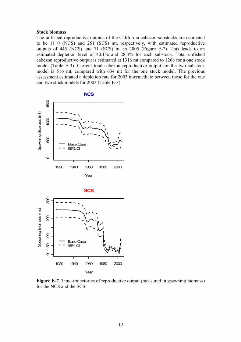
Stock biomass The unfished reproductive outputs of the California cabezon substocks are estimated to be 1110 (NCS) and 251 (SCS) mt, respectively, with estimated reproductive outputs of 445 (NCS) and 71 (SCS) mt in 2005 (Figure E-7). This leads to an estimated depletion level of 40.1% and 28.3% for each substock. Total unfished cabezon reproductive output is estimated at 1316 mt compared to 1268 for a one stock model (Table E-3). Current total cabezon reproductive output for the two substock model is 516 mt, compared with 634 mt for the one stock model. The previous assessment estimated a depletion rate for 2003 intermediate between those for the one and two stock models for 2003 (Table E-3).

1920 1940 1960 1980 2000

050

010

0015

00

NCS

Year

Spa

wni

ng B

iom

ass

(mt)

Base Case95% CI

1920 1940 1960 1980 2000

050

100

200

300

Year

Spa

wni

ng B

iom

ass

(mt)

Base Case95% CI

SCS

Figure E-7. Time-trajectories of reproductive output (measured in spawning biomass) for the NCS and the SCS.

12

Table E-3. Total cabezon reproductive output and depletion rates in California.

Model SB1916 SB1930 SB2003 SB2005 SB2003/SB1930 SB2005/SB1916

2005 Assessmenttwo substock model 1361 1353 542 516 40.0% 37.9%

one stock model 1268 1260 353 634 28.0% 50.0%2003 Assessment 902 313 34.7%

Total California Cabezon Spawning Biomass (mt)

Recruitment A Beverton-Holt equation with lognormal process error is used to characterize the spawner-recruitment relationship of cabezon. The steepness parameter is set to 0.7 for the base model. Recruitment residuals are estimated for 1980–2003 (NCS) and 1970–2003 (SCS). There are several major recruitment events for the NCS after 1980, but only two for the SCS: one in 2000 and another in 2003, both about twice the historical average (Figure E-8). Actual recruitment patterns are unclear because of a lack of age-composition data.

1920 1940 1960 1980 2000

050

010

0015

0020

00

NCS

Year

Rec

ruitm

ent (

1000

s)

1920 1940 1960 1980 2000

010

030

050

0

Year

Rec

ruitm

ent (

1000

s)

SCS

Figure E-8. Time-trajectories of recruitment (1000s) for the NCS and the SCS. Bold lines are point estimates; broken lines represent the approximate 95% confidence intervals.

13

Table E-4. Ten year summary of catches, biomass, recruitment and depletion levels for each of the cabezon substocks. Parenthetic values are asymptotic standard deviations.

NCSStatewide Total Exploitation Spawning Potential Summary Age Spawning Stock

Year OY (F50%) Catch Rate Ratio (SPR) (2+) Biomass Biomass Recruitment Depletion level1995 -- 125 13% 40% 779 382 (30) 437 (185) 34%1996 -- 170 17% 33% 917 362 (32) 687 (226) 33%1997 -- 206 20% 29% 909 380 (37) 876 (245) 34%1998 -- 250 25% 25% 895 393 (44) 206 (154) 35%1999 -- 127 14% 41% 876 356 (51) 1059 (274) 32%2000 72 119 12% 45% 849 393 (63) 171 (129) 35%2001 72 83 8% 56% 963 420 (74) 86 (56) 38%2002 81 74 8% 61% 959 466 (87) 118 (76) 42%2003 88 68 7% 63% 900 507 (101) 232 (165) 46%2004 69 73 9% 60% 815 496 (105) 554 (54) 45% (8%)2005 69 -- -- 731 445 (103) 541 (56) 40% (8%)

SCSStatewide Total Exploitation Spawning Potential Summary Age Spawning Stock

Year OY (F50%) Catch Rate Ratio (SPR) (2+) Biomass Biomass Recruitment Depletion level1995 -- 15 19% 29% 57 31 (4) 21 (17) 12%1996 -- 24 29% 17% 75 26 (4) 144 (37) 10%1997 -- 18 22% 23% 64 23 (4) 38 (25) 9%1998 -- 28 32% 16% 82 26 (4) 8 (7) 10%1999 -- 30 39% 14% 74 25 (4) 80 (29) 10%2000 72 30 39% 12% 52 23 (3) 398 (69) 9%2001 72 22 24% 12% 43 14 (3) 10 (7) 5%2002 81 18 15% 29% 116 12 (3) 38 (21) 5%2003 88 16 11% 47% 130 35 (7) 298 (93) 14%2004 69 13 7% 59% 135 60 (12) 105 (10) 24% (5%)2005 69 -- -- 191 71 (15) 111 (10) 28% (6%)

1920 1940 1960 1980 2000

0.0

0.5

1.0

1.5

NCS

Year

Spa

wni

ng d

eple

tion

Management targetMinimum stock size threshold

1920 1940 1960 1980 2000

0.0

0.5

1.0

1.5

Year

Management targetMinimum stock size threshold

SCS

Figure E-9. Time-trajectory (1916-2005) of spawning depletion for each substock in relation to management targets.

14

Exploitation status The current (2005) reproductive output of the cabezon resource off California is estimated to be about 40.1% and 28.3% of the unfished level based on the base models (Table E-4). The NCS, the major fished substock off California, seems healthy at this time, and is just above its target level (Fig. E-9). The status of the SCS is much more uncertain and sensitive to the exact specifications of the assessment, but its reproductive output is estimated to be more than 25% of the unfished level at present (Fig. E-9). Management performance No management regulations existed for cabezon before 1982 when a size limit (12-inches) was set for recreationally caught cabezon off California. This limit was raised to 14-inches in 2000, and extended to include commercially retained fish. It was increased further to 15-inches in 2001. Recreational bag limits have been 10fish/day in California since 2000. Cabezon are currently included in the California recreational regulatory complex Rockfish, Cabezon, and Greenlings (the RCG complex) and subject to seasonal closures for recreational fishers. Oregon imposed a 16-inch commercial size limit and a 15-inch recreational size limit for cabezon in 2001. Oregon has a 10fish/day bag limit for cabezon and greenling combined. California and Oregon are proposing slot limits for cabezon; cabezon must be between 15–22 inches in California and 15–19 inches in Oregon to be retained. There is no size limit in Washington and recreational fishers are limited to 15 bottom-type fishes daily. Historically, commercial landings of cabezon were monitored as part of a mixed group called “Other Fish”. This group of species includes sharks, skates, rays, grenadiers and other groundfish. This group has been defined historically as groundfish species that do not have directed or economically important fisheries. The coastwise ABC for this entire group of species was 14,700mt during 1999–2002 (5,200mt for the Eureka, Monterey and Conception INPFC areas and 9,500mt for the Columbia and Vancouver INPFC areas). In California, the cabezon fishery is independently monitored and regulated by analyzing two-month cumulative trip limits. In 2004, the season closed on 4 September when the annual commercial allocation of 75,600 pounds was reached before ends year. Regional Management The cabezon has thus far been managed on a coastwide basis in California. The results of this two substock assessment provide the scientific basis for cabezon to be managed regionally using the California Department of Fish and Game northern/central and southern California management areas. More work and sampling effort is needed to evaluate whether cabezon in these two areas differ biologically (growth, maturity, etc.), but the results of this assessment indicate that the biomass of cabezon in the southern management area may be smaller than that of conspecifics north of Point Conception. Regional management is an important consideration in relatively sedentary nearshore reef species such as cabezon and future assessments should continue to provide scientific analyses on increasingly finer spatial scales.

Forecasts Twelve-year yield forward projections are conducted for each substock under two alternative ABC control rules (based on FMSY proxies of F45% and F50%) and two OY

15

threshold control rules (40-10 or 60-20). The standard PFMC OY control rule for groundfish such as cabezon is based on F45% with a 40-10 adjustment for stocks below the target level of 40% of the unfished reproductive output. The California Nearshore Fishery Management Plan proposes the use of a FMSY proxy of F50% and a 60-20 adjustment for stocks below 60% of the unfished reproductive output. The relative proportion of the six fleets in future harvests is assumed to be the same as the last year (2004) in the model. Results of the projections are given in Table E-5. Table E-5. Summary of forecast outputs for the A) NCS and B) SCS. A) NCS

Year OY ABC SB2+ SB Depletion OY ABC SB2+ SB Depletion2005 59 107 727 440 40% 59 90 727 440 40%2006 59 90 684 393 35% 59 78 684 393 35%2007 84 81 655 360 32% 44 71 655 360 32%2008 76 78 655 327 29% 43 70 691 351 32%2009 77 81 684 321 29% 48 73 746 363 33%2010 84 86 721 335 30% 58 78 805 390 35%2011 91 92 755 354 32% 68 83 857 420 38%2012 97 96 782 370 33% 77 88 900 445 40%2013 102 100 803 383 34% 84 91 934 465 42%2014 105 103 821 392 35% 89 95 960 481 43%2015 108 105 834 400 36% 93 97 981 494 44%2016 110 107 845 406 37% 96 100 997 503 45%

B) SCS

Year OY ABC SB2+ SB Depletion OY ABC SB SB2+ Depletion2005 10 24 197 72 29% 10 21 197 72 29%2006 10 27 217 90 36% 10 23 217 90 36%2007 30 26 226 112 45% 22 23 226 112 45%2008 29 25 219 111 45% 22 23 227 116 46%2009 28 25 214 106 43% 21 23 228 115 46%2010 27 25 211 103 41% 21 23 230 115 46%2011 27 25 209 101 40% 22 23 232 116 46%2012 27 25 207 100 40% 22 23 234 117 47%2013 27 25 206 100 40% 22 24 235 118 47%2014 26 26 205 99 40% 23 24 237 118 47%2015 26 26 204 99 39% 23 24 237 119 48%2016 26 26 204 98 39% 23 24 238 120 48%

40-10/F45% 60-20/F50%

40-10/F45% 60-20/F50%

Decision table Projections based on alternative states of nature for each substock were explored to capture uncertainty in population conditions. For the NCS, the low and high M scenarios refer to different assumptions about sex-specific natural mortality and were selected to represent the 95% confidence intervals for terminal spawning biomass based on the Hessian approximation. The low scenario assumes M = 0.2yr-1 and 0.25 yr-1 for females and males respectively, while the high scenario assumes 0.3 yr-1 and 0.35 yr-1 respectively. For the SCS, the low and high scenarios are based on altering the CV on the mean weight avalue in the year 2000 for the man-made fleet. These states of nature attempt to capture the uncertainty in current depletion based on the uncertainty in the magnitude of the 2000 recruitment. Results from each of the states of nature are given in Table E-2.

16

Decision analysis population projections are provided in Table E6 for each state of nature and several state-dependent future catch series. The NCS will drop below the overfished threshhold if catch levels are based on the 40-10 rule and the high M scenario, but the true state of nature is either the base case or low M scenario. This also occurs if catches are based on the base case model but the low M state of nature is correct. All other scenarios lead to depletion levels above 25% in 2016. Under the 60-20 rule, only the high M catch with a low M true state of nature leads to a depletion level in 2016 below 25%. In the SCS, all combinations of catch and true state of nature under either control rule lead to a depletion level in 2016 larger than 25%. Table E-6. Decision analysis of different states of nature under different catch histories and fishery control rules for each cabezon substock. NCS 40-10/F45%

Year OY Spawning Biomass Depletion Spawning Biomass Depletion Spawning Biomass Depletion2005 59 323 30% 440 40% 637 49%2006 59 286 27% 393 35% 567 44%2007 40 256 24% 360 32% 523 40%2008 40 249 23% 353 32% 515 40%2009 43 255 24% 366 33% 536 41%

Catch based on 2010 49 273 26% 396 36% 583 45%Low M model 2011 55 293 28% 431 39% 637 49%

2012 60 312 29% 464 42% 687 53%2013 65 328 31% 493 44% 731 56%2014 68 342 32% 518 47% 769 59%2015 72 354 33% 540 49% 802 62%2016 74 364 34% 559 50% 829 64%2005 59 323 30% 440 40% 637 49%2006 59 286 27% 393 35% 567 44%2007 84 256 24% 360 32% 523 40%2008 76 222 21% 327 29% 490 38%2009 77 207 19% 321 29% 493 38%

Catch based on 2010 84 206 19% 335 30% 526 41%Base Case 2011 91 208 20% 354 32% 567 44%

2012 97 207 19% 370 33% 603 47%2013 102 202 19% 383 34% 634 49%2014 105 194 18% 392 35% 660 51%2015 108 184 17% 400 36% 683 53%2016 110 173 16% 406 37% 702 54%2005 59 323 30% 440 40% 637 49%2006 59 286 27% 393 35% 567 44%2007 157 256 24% 360 32% 523 40%2008 136 176 17% 283 25% 447 35%2009 134 129 12% 246 22% 422 33%

Catch based on 2010 142 101 9% 235 21% 433 33%High M Catch 2011 151 75 7% 229 21% 452 35%

2012 157 42 4% 218 20% 466 36%2013 161 5 1% 202 18% 475 37%2014 164 8 1% 184 17% 481 37%2015 166 0 0% 164 15% 486 37%2016 168 0 0% 144 13% 490 38%

State of NatureLow M (F= 0.2/M=0.25)

p = 0.18High M (F=0.3/M=0.35)

p = 0.24Base Case M (F=0.25/M=0.3)

p = 0.58

17

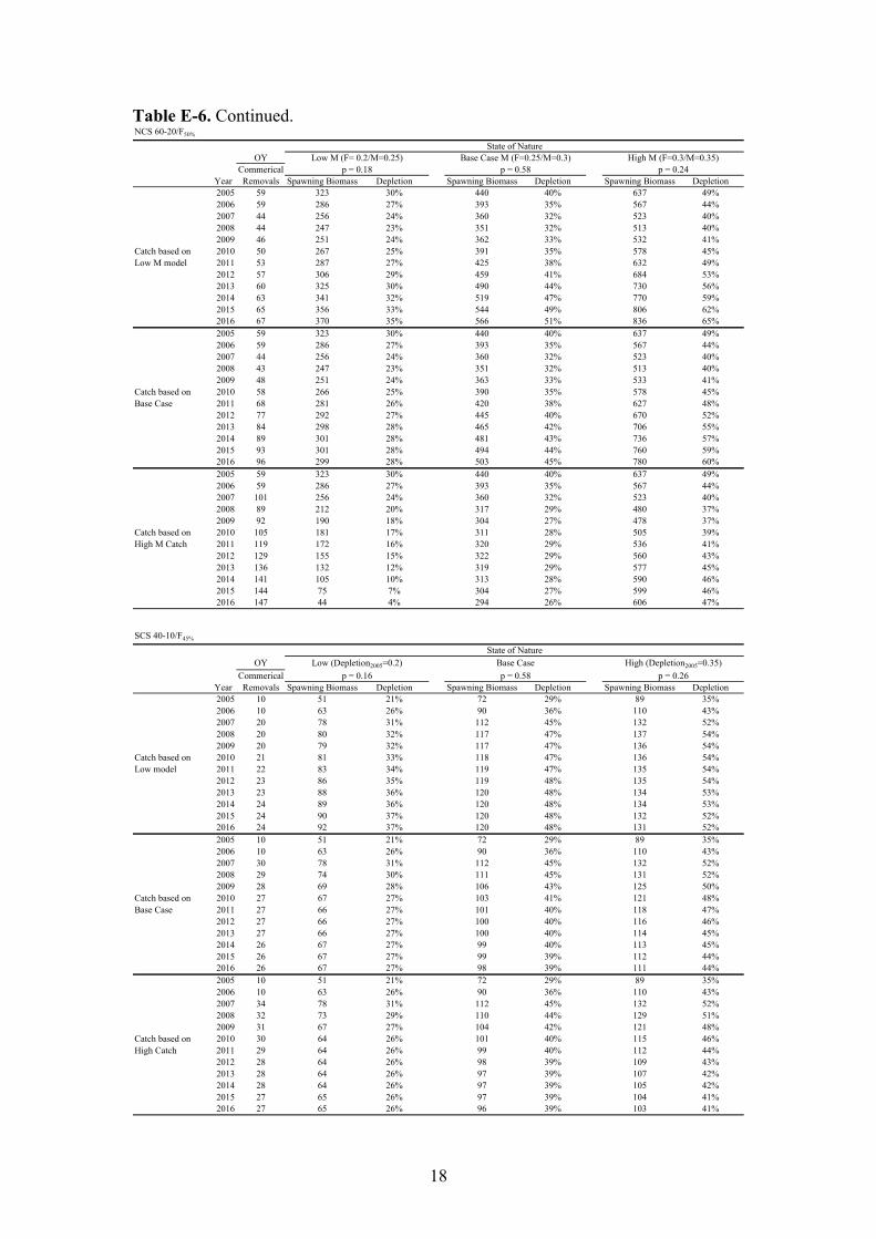
Table E-6. Continued. NCS 60-20/F50%

OYCommerical

Year Removals Spawning Biomass Depletion Spawning Biomass Depletion Spawning Biomass Depletion2005 59 323 30% 440 40% 637 49%2006 59 286 27% 393 35% 567 44%2007 44 256 24% 360 32% 523 40%2008 44 247 23% 351 32% 513 40%2009 46 251 24% 362 33% 532 41%


2012 57 306 29% 459 41% 684 53%2013 60 325 30% 490 44% 730 56%2014 63 341 32% 519 47% 770 59%2015 65 356 33% 544 49% 806 62%2016 67 370 35% 566 51% 836 65%2005 59 323 30% 440 40% 637 49%2006 59 286 27% 393 35% 567 44%2007 44 256 24% 360 32% 523 40%2008 43 247 23% 351 32% 513 40%2009 48 251 24% 363 33% 533 41%


2012 77 292 27% 445 40% 670 52%2013 84 298 28% 465 42% 706 55%2014 89 301 28% 481 43% 736 57%2015 93 301 28% 494 44% 760 59%2016 96 299 28% 503 45% 780 60%2005 59 323 30% 440 40% 637 49%2006 59 286 27% 393 35% 567 44%2007 101 256 24% 360 32% 523 40%2008 89 212 20% 317 29% 480 37%2009 92 190 18% 304 27% 478 37%


2012 129 155 15% 322 29% 560 43%2013 136 132 12% 319 29% 577 45%2014 141 105 10% 313 28% 590 46%2015 144 75 7% 304 27% 599 46%2016 147 44 4% 294 26% 606 47%

p = 0.18 p = 0.58 p = 0.24

State of NatureLow M (F= 0.2/M=0.25) Base Case M (F=0.25/M=0.3) High M (F=0.3/M=0.35)

SCS 40-10/F45%

OYCommerical


Catch based on 2010 21 81 33% 118 47% 136 54%Low model 2011 22 83 34% 119 47% 135 54%

2012 23 86 35% 119 48% 135 54%2013 23 88 36% 120 48% 134 53%2014 24 89 36% 120 48% 134 53%2015 24 90 37% 120 48% 132 52%2016 24 92 37% 120 48% 131 52%2005 10 51 21% 72 29% 89 35%2006 10 63 26% 90 36% 110 43%2007 30 78 31% 112 45% 132 52%2008 29 74 30% 111 45% 131 52%2009 28 69 28% 106 43% 125 50%


2012 27 66 27% 100 40% 116 46%2013 27 66 27% 100 40% 114 45%2014 26 67 27% 99 40% 113 45%2015 26 67 27% 99 39% 112 44%2016 26 67 27% 98 39% 111 44%2005 10 51 21% 72 29% 89 35%2006 10 63 26% 90 36% 110 43%2007 34 78 31% 112 45% 132 52%2008 32 73 29% 110 44% 129 51%2009 31 67 27% 104 42% 121 48%

Catch based on 2010 30 64 26% 101 40% 115 46%High Catch 2011 29 64 26% 99 40% 112 44%

2012 28 64 26% 98 39% 109 43%2013 28 64 26% 97 39% 107 42%2014 28 64 26% 97 39% 105 42%2015 27 65 26% 97 39% 104 41%2016 27 65 26% 96 39% 103 41%

Low (Depletion2005=0.2) Base Case High (Depletion2005=0.35)p = 0.16 p = 0.58 p = 0.26

State of Nature

18

Table E-6. Continued. SCS 60-20/F50%

OYCommerical



2012 18 103 42% 136 55% 152 60%2013 19 106 43% 138 55% 153 60%2014 20 109 44% 139 56% 152 60%2015 21 112 45% 140 56% 152 60%2016 21 113 46% 140 56% 151 60%2005 10 51 21% 72 29% 89 35%2006 10 63 26% 90 36% 110 43%2007 22 78 31% 112 45% 132 52%2008 22 79 32% 116 46% 136 54%2009 21 77 31% 115 46% 134 53%


2012 22 83 34% 117 47% 132 52%2013 22 85 35% 118 47% 132 52%2014 23 87 35% 118 47% 132 52%2015 23 89 36% 119 48% 132 52%2016 23 91 37% 120 48% 131 52%2005 10 51 21% 72 29% 89 35%2006 10 63 26% 90 36% 110 43%2007 27 78 31% 112 45% 132 52%2008 26 76 31% 116 46% 133 53%2009 25 72 29% 115 46% 128 51%


2012 24 74 30% 117 47% 123 49%2013 24 75 31% 118 47% 123 49%2014 23 77 31% 118 47% 123 49%2015 23 79 32% 119 48% 123 49%2016 23 80 33% 120 48% 122 49%

State of Nature

p = 0.16 p = 0.58 p = 0.26Low (Depletion2005=0.2) Base Case (F=0.25/M=0.3) High (Depletion2005=0.2)

19

Research Recommendations 1. Accurate accounting of removals, especially from the recreational and live-fish fisheries: Fisheries primarily exploited by recreational and live-fish commercial fisheries are traditionally hard to monitor. More effort to monitor these fishery sectors may be necessary to accurately monitor fishing mortality. 2. A fishery-independent survey of cabezon population abundance: The current fishery-independent survey being developed in the Morro Bay area will become an important input into future assessments of cabezon. Expansion of this survey will increase its usefulness as an index of abundance for central and northern California. 3. A study of the stock structure of cabezon: This assessment assumes two substocks of cabezon along the California coast. Current work on cabezon stock structure should be included in the next assessment. 4. Age validation/ age determination: Catch age-composition data were not available for this assessment. Accurate ageing is crucial to understand the population dynamics of a species, especially those for which there is limited survey information. Information on the age-structure of the catches for each fishery sector would substantially improve some aspects of the assessment. 5. A better understanding of the relationship between CPUE and population size: Changes in recreational CPUE indices are assumed to reflect changes in population size in a linearly proportional manner. The results of the assessment would be severely in error if this assumption were substantially violated. Therefore, if future assessments depend on CPUE data, it is vital that the relationship between CPUE and population size be quantified. 6. Alternative assessment procedures: The need for greater spatial resolution in the management of nearshore fisheries also increases the amount of data required to perform traditional stock assessments. Alternative assessment procedures that are less data-hungry, but still provide relevant management outputs should be developed to address this need. In addition, the nest-guarding behavior of males gives new values to males in the cabezon population. Another metric other than spawning biomass may be needed to help account for the male portion of the population in reference points. 7. Effect of climate on cabezon: Several of the data sources in this assessment (e.g. the power-plant impingement and CalCOFI indices, and some length-composition data) indicate that there was potentially good recruitment after 1999 (and before 1977 for the impingement data) whereas these same sources indicate that recruitment was very poor prior to 1999 in the SCS. Cabezon may be influenced by climatic/oceanic regimes. A better understanding of the relationship between cabezon population dynamics and climate would reduce the uncertainty of future assessments. 8. Sex-specific data: Given the strong correlation of color to gender in cabezon (O’Connell 1953; Lauth 1987; Grebel 2003), collection of sex-specific information (at least recording fish color) would greatly enhance future assessments.

Purpose

This is the second assessment of the population status of cabezon (Scorpaenichthys marmoratus [Ayres]) along the California coast (Figure 1). Although commercial removals of cabezon have increased off Oregon in recent years because of the live-fish fishery (ODF&W 2002), and substantial recreational catches of cabezon occur in both Oregon and Washington waters (Cope et al. 2004), the available data sources remain insufficient to form the basis for a reliable assessment of cabezon in those areas. The current assessment is intended to provide information that will be of use by managers at both the state and federal levels. This document follows, to the extent possible given the available information, the Terms of Reference for stock assessments established by the PFMC Scientific and Statistical Committee. Two objectives are addressed in this document. First, the life history of cabezon is described and all the available data sources that were considered for use in the assessment are explained. This document only provides detailed information for those data sources that were considered for use in the population modeling. Many other sources of information were considered, but ultimately rejected, and are not included in this document for brevity. Second, the document describes the results of the use of a new stock assessment technique (Stock Synthesis 2 [SS2], Methot 2005), and summarizes how the results from SS2 relate to those based on the assessment technique used for the 2003 assessment (the OC model). Unlike the 2003 assessment, increased attention is given to the spatial structure of the data for cabezon off California, with the consequence that the analyses of this document are based on two putative populations (“substocks”) separated at Point Conception, CA.

This assessment differs from those performed for most other west coast groundfish species because there is no fishery-independent index of abundance that covers the range of the stock. It consequently relies on indices of abundance based on recreational CPUE and spatially-restricted fishery-independent data, and information about larval and recruit abundance. Although no state- or federally-funded biomass indices are currently available for this species, these alternative data sources are considered to be adequate for estimating the values of the parameters of a population dynamics model. Much uncertainty remains in regard to the assumption that changes in recreational CPUE are linearly proportional to changes in population size. There is no information on the age-structure of the catches. Therefore, although the model is age-structured, it is fit to mean weights and length-composition data by converting the model-predicted catch age-compositions to catch size-compositions using growth curves and weight-length relationships.

21

Acronyms used in this document: ABC – Allowable Biological Catch AIC – Akaike Information Criterion CalCOFI - California Cooperative Oceanic Fisheries Investigation CalCOM - California Commercial Cooperative Groundfish Program CDF&G – California Department of Fish and Game CPFV – Commercial Passenger Fishing Vessel CPUE – Catch per unit of effort CRFS – California Recreational Fisheries Survey CV – Coefficient of variation EEZ – Economic Exclusive Zone FMP – Groundfish Fishery Management Plan GLM – Generalized Linear Model IRI – Index of Relative Importance MODE – Fishing Method (shore, private boat, charter boat) MPD – Maximum of the posterior density function MRFSS - Marine Recreational Fisheries Statistics Survey NCS – Northern California Substock NFMP – Nearshore Fishery Management Plan NWFSC – Northwest Fisheries Science Center OC – Original Cabezon model used in the 2004 assessment PBR – Private Boat and Rental PFEL – Pacific Fisheries Environmental Laboratory PFMC – Pacific Fishery Management Council PSFMC – Pacific States Marine Fisheries Commission RecFIN – Recreational Fisheries Information Network SCS – Southern California Substock SS2 – Stock Synthesis 2 SWFSC – Southwest Fishery Science Center WAVE – Bi-Monthly period of catches OY- Optimum Yield

22

Introduction The cabezon (Scorpaenichthys marmoratus) is the largest member of the family Cottidae (commonly referred to as sculpins) found in the waters along the Northeast Pacific. Cabezon are desired by both commercial and recreational fishers because of their great size, physical attractiveness, and tasty flesh. Current knowledge of cabezon life history is sparse, and is usually based on information collected from a limited extent of the range of the species. The population status of cabezon in California waters was assessed in 2003, and the spawning output was estimated to be less than 40% of the unfished spawning output, but there was considerable uncertainty (Cope et al. 2004). Cabezon are currently managed as part of a nearshore complex of fishes that include several species of rockfishes and greenlings.

This is the second quantitative assessment of the population status of cabezon. In an attempt to enhance the spatial resolution of the assessment, it is based on two putative populations (“substocks”) of cabezon in California, delineated at Point Conception, CA (Figure 1). Available data for the Oregon and Washington remain insufficient to form the basis for a reliable stock assessment for cabezon in these areas. Stock Structure There is little direct information on the stock structure of cabezon off the U.S. west coast. The genetic structure of cabezon is being investigated at California Polytechnic State University at San Luis Obispo, but no results are presently available (Dr. Royden Nakamura, pers. comm.).

The need for more spatial resolution in the assessment of cabezon was identified by the STAR panel that reviewed the past assessment. Distinct fishing histories, the distribution of fishing effort north and south of Point Conception, and the ecology of nearshore fishes, also indicate the need for a more spatially-resolved cabezon assessment. Specifically, the live-fish fishery for cabezon is active primarily north from the Morro Bay while, historically, the recreational take of cabezon has been greatest in central California, with the removals off southern Californian being fairly low. Cabezon are a cooler-water species, and are more abundant in the central and northern Californian nearshore areas. Typical of nearshore reef fishes, cabezon subpopulations are often spatially discrete, and therefore susceptible to serial depletion, which suggests the need to examine population trends at small spatial scales. The extent to which assessments can be conducted at small spatial scales is, however, limited. Nevertheless, it is possible to treat the cabezon resource off California as two populations (or “substocks”; the Northern California Substock (NCS) and the Southern California Substock (SCS)) with a division at Point Conception (Figure 1). This assessment accordingly reflects California-specific management needs by separating the central and northern management areas from the southern management area (Figure 1). One could also argue for an additional division north of Punta Gorda (the CDF&G Northern California Region) because of its unique fishing history, but there are currently insufficient data to support such a division. This assessment also explores the implications of assessing the entire cabezon resource off California as a single homogeneous resource to determine some of the impacts of allowing for spatial resolution.

23

Life History Distribution Cabezon is distributed along the entire west coast of the continental United States. It ranges from central Baja California north to Sitka, Alaska (Quast 1968; Miller and Lea 1972; Love et al. 1996). Cabezon are primarily a nearshore species found intertidally and among jetty rocks, out to depths of greater than 100 m (Miller and Lea 1972; Love et al. 1996). The majority of the commercial and recreational catch is taken inside of 15–20fm (and approximately 99% within 30fm; Feder et al. 1974) and along the central California coast up through Oregon. Species Associations Cabezon is a member of a nearshore assemblage of fishes that includes several Sebastes species (e.g. S. atrovirens, S. auriculatus, S. carnarus, S. caurinus, S. chrysomelas, S. dallii, S. maliger, S. melanops, S. mystinus, S. nebulosus, S. rastrelliger, S. serranoides, and S. serriceps), kelp (Hexagrammos decagrammus) and rock greenling (H. lagocephlaus), monkeyface prickleback (Cebidichthys violaceus)), California scorpionfish (Scorpaena guttata), and California sheephead (Semicossyphus pulcher). These 19 fishes are included in California’s Nearshore Fishery Management Plan (CDF&G 2002), an FMP required by mandate of the 1999 Marine Life Management Act. At present, only cabezon, California sheephead (Alonzo et al. 2004), and black rockfish (Ralston and Dick 2003) have been assessed, although gopher rockfish, kelp greenling, and California scorpionfish are scheduled to be assessed during 2005. Spawning and Early Life History Cabezon are known to spawn in recesses of natural and manmade objects, and males are reported to show nest-guarding behavior (Garrison and Miller 1982). Spawning is protracted, and there appears to be a seasonal progression of spawning that begins off California in winter and proceeds northward to Washington by spring. Spawning off California peaks in January and February (O’Connell 1953) while spawning in Puget Sound (Washington State) occurs for up to 10 months (November-August), peaking in March–April (Lauth 1987). Laid eggs are sticky and adhere to the surface where deposited. After hatching, the young of the year spend 3–4 months as pelagic larvae and juveniles. Settlement takes place after the young fish have attained 3–5 cm in length (O’Connell; 1953; Lauth 1987). It is apparent that females lay multiple batches in different nests, but whether these eggs are temporally distinct enough to qualify for separate spawning events is not understood (O’Connell 1953; Lauth 1987). The number of eggs spawned appears to increase with fish size (weight or length) (O’Connell 1953; Lauth 1988). However, the actual relationship between age / size and number of eggs spawned is uncertain because of the possibility of multiple spawnings. Therefore, rather than attempting to determine this relationship, the reproductive output has, for the purposes of this assessment, been defined to be proportional to the product of maturity-at-age and body weight at the start of the year. Maturity ogives (Figure 2; Table 1) were estimated using the California Department of Fish and Game (CDF&G) visual inspection codes and the data used by Grebel (2003). Females with gonads with early yolk stage eggs were assumed to be mature, although it is possible that some of these fish were maturing, but not yet mature. This

24

will lead to a more optimistic interpretation of the rate at which cabezon mature (younger and at smaller size).

Age and Size relationships Cabezon are among the largest of the cottids, attaining a length of nearly 1m and a weight in excess of 11 kg (Feder et al. 1974). Female cabezon are larger than males of the same age (Figure 3A). O’Connell (1953) provided the first estimates of cabezon age and growth using whole otoliths from specimens from central and southern California. Lauth (1987) provided another estimate of cabezon growth from the Puget Sound (WA) using several ageing structures (whole otoliths, sectioned fin rays). Finally, Grebel (2003) conducted a comprehensive study (almost 700 individuals collected over 6 years) on age and growth of cabezon from California using several age structures (sectioned otoliths, pectoral fin rays, dorsal fin rays, dorsal spines, and vertebrae). Her results using a thin-section of the saggital otolith form the basis for a growth curve for cabezon in this assessment. Ages from Grebel (2003) were all standardized to a 1 January birthdate to avoid bias caused by rapid growth during the first years of life, and von Bertalanffy growth curves were fitted to the resulting age-length data (Table 1). Partial “validation” of this growth curve was achieved by estimating the values for and k from tag-recapture data (K. Karpov, CDF&G, pers. comm.) and setting so as to minimize the sums of squares of size-at-age for the combined sexes and the tag-recapture estimates. The ageing- and tagging-based growth curves do not appear to be in conflict (Figure 3B). Because Grebel (2003) found no biologically significant differences between the age-at-length relationships among regions (northern, central, and southern) in California, her sex-specific results are used for both substocks in this assessment. The growth curves obtained by Grebel (2003) differed statistically from that of O’Connell’s (1953), who had much larger individuals in his samples. Whether these differences in estimated age-length relationships derive from an ageing disparity between whole and sectioned otoliths, or they represent real differences caused by changes in the population structure (possibly due to fishing) is purely speculative at present, and is therefore not considered further in this assessment.

L∞

0t

Weight-length relationships for cabezon are provided in O’Connell (1953; central California), Lauth (1987; Puget Sound, WA), and Lea et al. (1999; central California) for both sexes combined. Lea et al. (1999) also provide relationships for females and males separately, but for central California only. Raw length-weight data used in Grebel (2003) provide substock- and sex-specific length-weight information with larger sample sizes than the earlier studies, and these data are used for the present assessment (length in cm and weight in kg; Table 1). Sampling effort covered the years 1993–2002 for the NCS, and 2002 for the SCS. Natural Mortality (M) Little is known about the natural mortality rate of cabezon, so empirical methods using life history traits (growth rate (k), age-at-maturity (aM), maximum age (ω)) were used to estimate natural mortality. The previous assessment used the method of Hoenig (1983) to estimate a common M for both sexes. The STAR panel that reviewed the 2003 assessment suggested that this assessment address sex-specific natural mortality rates because of differential growth between the sexes. Five methods for estimating M (Hoenig 1983; Chen and Watanabe 1989; Jensen 1996) were therefore applied to data for each sex, and the results averaged to obtain sex-specific

25

natural mortality rates (Table 2). The mean of these approaches imply a natural mortality rate of approximately 0.25 yr-1 for females and 0.3 yr-1 for males, but these methods may produce highly uncertain values of M (Pascual and Iribarne 1993). Therefore, sensitivity to the assumed values of M is explored when applying the assessment model. Fisheries History

Historically, the recreational sector has been the main source of cabezon removals. Cabezon have been a very minor component of the catch in commercial fisheries for more than a century (Jordan and Everman 1898). The earliest modern commercial fishery information (O’Connell 1953) indicates that a small amount of cabezon was being sold in fish markets in the San Francisco area by the 1930s with incidental take recorded back to 1916. However, it was not until the 1990s that a truly directed commercial fishery for cabezon was established in the waters of California and Oregon. The most significant change in the fishery for cabezon has been the development of the live-fish/premium commercial fishery that, in addition to cabezon, targets several other nearshore fishes (CDF&G 2002). This fishery started in southern California in the late 1980s and spread northward during the late 1990s to Oregon (Starr et al. 2002). Fishermen routinely obtain much higher prices for fish brought back to markets alive. Cabezon are not subject to barotrauma because they lack a swim bladder and are usually found in shallow nearshore waters accessible to many fishers. These traits make cabezon an ideal target for both the live-fish and recreational fisheries. Gears that take cabezon include hook and line and pot/trap type gears, as they are successful at bringing up fish with relatively little damage. Cabezon continues to be an important component of the live-fish fishery, even with increased restrictions on the live-fish catch, especially as the allowable catches of other marketable groundfish species have been reduced. Fisheries Management The Pacific Fishery Management Council (PFMC) and NOAA Fisheries have management responsibility for the groundfish species included in the Groundfish Fishery Management Plan (FMP) out to the boundary of the 200-mile Exclusive Economic Zone (EEZ). Many nearshore species, such as cabezon, that fall primarily within the 3-mile limit of states’ waters are also included in state-specific Nearshore Fishery Management Plans (NFMP). NFMPs are currently being developed and implemented in California and Oregon in response to the increased commercial take of the live-fish fishery (CDF&G 2002) No management regulations existed for cabezon before 1982 when a size limit (12-inches) was set for recreationally caught cabezon off California (see Appendix A for a complete list of California regulations). This limit was raised to 14-inches in 2000, and extended to include commercially retained fish. It was increased further to 15-inches in 2001. Recreational bag limits have been 10fish/day in California since 2000. Cabezon are currently included in the California recreational regulatory complex Rockfish, Cabezon, and Greenlings (the RCG complex) and subject to seasonal closures for recreational fishers. Oregon imposed a 16-inch commercial size limit and a 15-inch recreational size limit for cabezon in 2001. Oregon has a 10fish/day bag

26

limit for cabezon and greenling combined. California and Oregon are proposing slot limits for cabezon; cabezon must be between 15–22 inches in California and 15–19 inches in Oregon to be retained. There is no size limit in Washington and recreational fishers are limited to 15 bottom-type fishes daily. Historically, commercial landings of cabezon were monitored as part of a mixed group called “Other Fish”. This group of species includes sharks, skates, rays, grenadiers and other groundfish. This group has been defined historically as groundfish species that do not have directed or economically important fisheries. The coastwise ABC for this entire group of species was 14,700mt during 1999–2002 (5,200mt for the Eureka, Monterey and Conception INPFC areas and 9,500mt for the Columbia and Vancouver INPFC areas). In California, the cabezon fishery is independently monitored and regulated by analyzing two-month cumulative trip limits. In 2004, the season closed on 4 September when the annual commercial allocation of 75,600 pounds was reached before ends year.

Assessment Data Sources

Data for species managed by NOAA Fisheries and the Pacific Fishery Management Council are collected by both federal (and/or quasi-federal) and state agencies. This can complicate analysis because several agencies may collect the same types of data. Where this occurs, the analyses below are based on those data that are most likely to be informative regarding changes in population size.

Removals Whenever possible, removals are characterized as landed catch plus fish released and presumed dead. Historical catches (prior to 1980) are reconstructed from historical documents, and reported and inferred relationships among fishing sectors. This is a change from the approach of inferring historical catches from state reports or backward projections of more recent catches as was done for the 2003 assessment. Recreational Fishing History in California Recreational fishing in California became popular in the late 1890s, but was limited to mostly big game fishes (tuna, marlin, and swordfish) and wealthy participants (Holder 1914). There remained in California limited recreational fishing opportunities to most people before 1920. Private boat access to nearshore fishes increased after 1920 (Croaker 1939), but it was not until Commercial Passenger Fishing Vessels (CPFVs) began operating in earnest off southern California in 1928 that the general public gained extensive accessibility to many nearshore fishes (Scofield 1928; Young 1969). Both barges – large, flat, open-spaced ships – and more traditional CPFV boats comprised the fleet. There were 15 barges and 20–30 boats off southern California in 1928 (Scofield 1928). The period 1929–39 saw a rapid increase in the popularity of CPFVs (Fig. 4; Croaker 1939), which also spread northward to central and northern California. By 1932, sportfishing in Monterey was very popular, with cabezon a major target species (Classic 1932). Pier and shore fishing modes also provided major recreational fishing outlets during this time of increased CPFV activity (Scofield 1928; Croaker 1938; Baxter & Young 1953; Young 1969). In all modes, most fishing occurred during the summer and autumn months, with some fishing extending into spring (Fry 1932; Baxter & Young 1953). CPFV captains have been required to submit logbooks detailing catches since 1936 (Croaker 1939; Baxter & Young 1953;

27

Young 1969), although compliance rates were and are not 100%. In 1937, the sportfishing catch exceeded the commercial catch for many species (Conner 1937).

The popularity of CPFV fishing continued to increase until the war years of 1942–46 when CPFV activity was considerably reduced (Fig. 4; Calhoun 1950). The CPFV fleet underwent a period of rapid re-establishment, reinvention, and growth after 1946 (Young 1969). Fleets, boat size, and passenger interest all increased throughout California. This expansion continued into the 1970s with the fleet peaking in 1973 (Baxter & Young 1953; Young 1969; Hill & Schneider 1999). A concomitant increase in private boat, shorefishing, and pier/jetty modes also occurred during this time, particularly in central California (especially in Monterey and Morro Bay), where cabezon are well represented, during the 1950s (Baxter & Young 1953). Reconstructing Recreational Removals This assessment uses a reconstructed catch history back to 1916 for both cabezon substocks. This initial year was selected because of the availability of commercial catches back to 1916 (see Reconstructing Commercial Removals below). Four recreational fishing modes are distinguished: 1) Man-made (piers/jetties), 2) Shore (beach/bank), 3) Private Boat and Rental (PBR), and 4) CPFV. These modes were distinguished for analysis and modeling purposes because of differences in selectivities and the length-frequency of the catch: the man-made and shore modes generally catch smaller individuals than the PBR and CPFV modes. Most cabezon are taken from jetties in the man-made mode (Pinkas et al. 1967). There was almost certainly very little recreational catch before 1916 so the fishing mortalities before 1916 for the four recreational modes are set to zero when conducting the assessment.

Information on the activities of recreational fishermen is collected by both state (CDF&G) and federal (MRFSS) programs. Since 1980 (excluding the years 1990–92), the MRFSS program (available via the RecFIN database: http://www.psmfc.org/recfin/) provides effort information from a random-digit dialing protocol and catch/trip information from intercept interviews. These data can be used to calculate total catches by mode. In 2004, the CDF&G, in cooperation with the PSFMC, started the California Recreational Fisheries Survey (CRFS) program to replace the MRFSS sampling program in California for all modes. This program aims to increase sampling effort for better catch and effort estimation, to increase spatial resolution of catches, and to identify targeted species. Before the CRFS was implemented, CDF&G only collected logbook catches from the CPFV fishery. Very few estimates of the removals by the man-made, shore, and PBR modes are available for the years before 1980. The CPFV fleet therefore provides the longest time-series of measured catches (1936-present) and is used to reconstruct the removals by the other three modes for the years prior to 1980.

Total recreational removals for each cabezon substock for each recreational mode were reconstructed in three steps: 1) the historical CPFV removals (in numbers) were reconstructed, 2) the CPFV removals were used to estimate the removals (in numbers) by the other three modes, and 3) the average weights per mode were used to estimate total removals in kg.

1. Historical CPFV removals The historical CPFV catch (1916–2004) was reconstructed as follows:

28

http://www.psmfc.org/recfin/

• Year 2004: CRFS database, extracted 17 February, 2005. • Years 1957–78; 1980–2003: Hill and Schneider (1999) performed a data

recovery exercise to extract catch, effort, block (CDF&G designated 10 x 10 nautical mile statistical areas), and month information from the California CPFV logbooks. This information provides area-specific catches (in numbers) for each cabezon substock for 1957–2003, excluding 1979 (the data for this year are lost). This data set was obtained on 24 January, 2005.

• Year 1979: Oliphant et al. (1990) report the total catch of cabezon by the CPFV fleet for 1979. This total is allocated to substock using the geometric mean of the ratio CatchNCS:CatchSCS for 1976–78 and 1980–82.

• Years 1936–40; 1947–56: Hill and Schneider (1999) provide CPFV catches for the SCS only. The total California CPFV catches for these years are found in Best (1963). The difference between total California catches and the catches from the SCS give the catches from the NCS.

• Years 1941–46: O’Connell (1953) provides the catch by the CPFV fleet in 1946 for each substock. No data are available for 1941–45; the catches during these years have been assumed equal to that for 1946.

• Years 1928(SCS)/1929(NCS)–1935: No data on catches are available for these years. Scofield (1928) identified the major start of the CPFV fleet in southern California to be 1928, which then moved into central and northern California in 1929 (Young 1929). These start years reflect the beginning of the CPFV time-series for the SCS and NCS, respectively. A linear increase in catch from the start year through 1935 is assumed because the CPFV fleet is known to have increased rapidly during these years (Fry 1932; Young 1969),

• Years 1916–27(SCS)/–1928(NCS): The catches by the CPFV fleet were assumed to be zero for these years.

Heimann & Miller (1970) reported that cabezon are rarely discarded in the CPFV fishery because of their large size and trophy status. Furthermore, discarded cabezon have a higher probability of survival because they are not affected by barotraumas. Even though a size limit has been imposed in recent years (see Appendix A), the analyses of this document assume that there is no discard mortality by the recreational sector. The reconstructed raw CPFV catches are shown in Fig. 5.

It was recognized early in the CPFV reporting process (Croaker 1938; Baxter & Young 1953) that logbook records may be inaccurate for two main reasons: 1) mis-reporting of catches (either over- or under-reporting; Karpov et al. 1995), and 2) less than 100% reporting compliance rates (Hill & Barnes 1998). Baxter & Young (1953) investigated these inaccuracies in CPFV catch and concluded that cabezon catch rates reported by the CPFV fleet are accurate and reliable. Reported CPFV removals are therefore not adjusted for mis-reporting. Since 1936, compliance rates have always been less than 100% though, and necessitate the adjustment of raw CPFV removals. Compliance rates (as reported from several sources) are provided in Table 3 and were assumed to be the same for the NCS and the SCS fleets. The reported compliance rates were then used to interpolate compliance rates for the years for which rates were not available, and CPFV removals in numbers were expanded to correct for lack of reporting compliance (Fig. 6). There are no compliance rates for the period 1962–1980. Values used for these years were semi-arbitrarily set to account for the expanding fleet during the 1960s and 1970s.

29

2. Estimating removals for the man-made, shore, and PBR modes via CPFV ratios Removals (in numbers) for the other three recreational modes (man-made, shore, and PBR) were determined in two ways: 1) based on surveys of the modes, and 2) based on an estimate of the ratio of the catch by the mode to the catch by the CPFV mode multiplied by the catch by the CPFV mode. Surveys are available for only a small numbers of years:

a) the RecFIN database contains estimates of removals for the years 1980–89 and 1993–2004 (2004 via CRFS). This data was extracted 17 February, 2005.

b) Miller & Gotshall (1965) provide estimates of NCS removals for the period 1957–61.

The ratios of the CPFV catches to the catches by the other modes from RecFin were used to estimate removals when data were missing for the years 1980–2004 (Tables 4 & 5). The work of Miller & Gotshall (1965) and Pinkas et al. (1968) provide ratios for the years of their study (Tables 4 & 5). These ratios were used to make inferences about the ratios for the years for which no data are available. The PBR fishery was assumed to start in the same year as the CPFV fishery. The man-made and shore modes began before the CPFV fishery, so the estimated catch in these modes for the years before the CPFV fishery began were projected back to 1916. 3. Calculating removals in kg The average annual weight of the removals (in kg) for each mode are given in Tables 4 and 5 for the NCS and SCS respectively, with shaded values indicating reported weights. The reported weights for 1980–2004 are taken from RecFIN. The reported weights for the NCS for the years before 1980 are: 1) 1947–51: Baxter & Young (1953) and 2) 1957–61: Miller and Gotshall (1965), while the reported values for the SCS for 1964–66 taken from Pinkas et al. (1968). The weights for all remaining years are assumed values, based on these sources, averaged RecFIN weights, or a mid-point of the two (Table 4 & 5). The weights for the PBR mode for the years prior to 1980 are set to those for the CPFV mode because these fisheries catch similar sized fish. The removals in the NCS by mode are heaver on average than those in the SCS. Removals (in kg) were calculated by multiplying numbers by average weights. The total removals (in kg) by the recreational sector by mode are shown in Figure 7 and by sub-stock in Figure 8A. Figure 8B compares the total recreational removals (in kg) between the current and the 2003 assessment. Despite the complete reconstruction of the removals by the recreational sector, the two series of catches are not notably different. Removals in weight were converted to metric tons before being included in the assessment model.

Sensitivities to assumed pre-1980 removals The removals are considered known without error in the assessment, but the above reconstruction is subject to considerable uncertainty. Two types of sensitivity tests are considered to examine the implications of this uncertainty: 1) using numbers instead of biomass for the recreational removals, and 2) doubling and halving the pre-1980 removals.

Recreational catch in 1980 The 2003 assessment and subsequent STAR panel identified the extraordinarily high recreational removal for 1980 as an area for further investigation. Figure 7 reveals that the high 1980 removal is attributed primarily to the catch by the PBR mode from the SCS. Further investigation reveals that RecFIN waves (i.e. bi-monthly totals) 1, 2, 3,

30

and 5 have notably higher removals (in kg) in 1980 than during 1982–89 (Figure 9, upper panel), but that average wave weights are not markedly different among years (Figure 9, lower panel).

Commercial Catches Several sources of California commercial landings are available to reconstruct commercial cabezon landings by substock back to 1916 (the first year of required reporting in the commercial fishery):

• Years 1978–2004: The CalCOM database provides annual landings (in pounds) by gear. Data was extracted on 19 April, 2005.

• Years 1930–77: The Pacific Fisheries Environmental Laboratory (PFEL) live access server (http://las.pfeg.noaa.gov:8080/las_fish1/servlets/dataset) and the California Explores the Ocean (http://ceo.ucsd.edu/fishcatchtables/fish-catch-download.html) website provide electronic summaries of CDF&G fish ticket receipts originally reported in the Fish Bulletin series (available electronically at: http://ceo.ucsd.edu/fishbull/). These sources were compared with landings in the Fish Bulletin publications and found not to be different for these years. All landings are reported in pounds. Data was obtained on 8 March, 2005.

• Years 1916–29: The publication California Fish and Game (vols 1–16) are the original source of landing reports before the Fish Bulletin series and are used for this time period. During 1916–29, cabezon was included in the category “sculpin” which included the California scorpionfish. Given the limited northern range of the scorpionfish (Love et al. 1987), 100% of the “sculpin” catch from Monterey north was assumed to be cabezon. Fish Bulletins 74 (CDF&G 1949) and 149 (Heimann and Carlisle 1970) provide summarized commercial cabezon landings for 1916–47 and 1916–69 respectively and were used to cross-compare cabezon catches from the California Fish and Game volumes. Both sources provided the same estimates of total cabezon landings.

• Years 1916–77 adjusted: The spatial resolution of landings from the CalCOM database is sufficient to separate landings into substocks. All other sources used the port complex “Santa Barbara” which included Morro Bay of the NCS and Santa Barbara of the SCS. Landings in the “Santa Barbara” port complex are therefore allocated to substock using the geometric mean of the ratio of the Morro Bay to Santa Barbara landings for the years 1978–82 from CalCOM (Figure 10).

Finally, total cabezon landings in pounds were converted into metric tons. Two fleets are distinguished for assessment purposes: 1) non-live, and 2) live. Cabezon commercial landings for each substock are given in Table 6. California landings of cabezon were low until the early- to mid-1990s when the live-fish/premium finfish fishery began targeting cabezon (Fig. 11). Commercial cabezon landings reached a peak of over 150mt in 1998 and averaged more than 80mt since the mid-1990’s, most of which came from the NCS (Fig. 12A). There is no discernable difference between the commercial landings in the present assessment and those used in the 2003 assessment (Fig. 12B).

31

http://las.pfeg.noaa.gov:8080/las_fish1/servlets/dataset

http://ceo.ucsd.edu/fishcatchtables/fish-catch-download.html

http://ceo.ucsd.edu/fishcatchtables/fish-catch-download.html

http://ceo.ucsd.edu/fishbull/

Cabezon are caught commercially using a variety of gears-types, but have been taken almost exclusively by hook-and-line and pots recently (Fig. 13). All catches are assumed to be taken using a single gear-type for the purposes of this assessment.

There have also been spatial and temporal patterns in cabezon commercial landings. Historically, much of the landings were reported in the late winter/early spring months, but much of the catch has been taken in the summer and fall months since the start of the live-fish fishery (Fig. 14). Currently, no commercial fishing for cabezon is allowed in March and April. All catch is assumed to be taken in the middle of the year for the purposes of the assessment. Figure 15 shows the port complexes affiliated with commercial cabezon landings. The “Santa Barbara” complex contains both Morro Bay and Santa Barbara, with Morro Bay contributing the most to the recent live-fish fishery catch. All NCS ports report higher commercial landings than either of the SCS ports.

Commercial Discards Discard mortality is assumed to be negligible for the purposes of this assessment because of the shallow habitat of this fish, its physiology, and its hardiness. The lack of any appreciable cabezon discard in the West Coast Groundfish Observer Program (WCGOP 2005) supports this assumption. Further information regarding discards in the nearshore life-fish fishery is being collected by the West Coast Groundfish Observer Program, but this information was not available for this assessment (J. Cusick, pers. comm.)

Total Removals Given the nearshore depth-distribution and latitudinal range of cabezon, it is not surprising that the bulk of the historical removals are by the recreational sector north of Point Conception (Fig. 16). Recently though, the landings by the live-fish fishery have surpassed those by the recreational fishery as the main source of cabezon removal. Total removals (kg) used in the current assessment are not noticeably different from those used in the 2003 assessment, particularly for recent years (Fig. 16).

Size Compositions Cabezon otoliths and other ageing structures have not been collected routinely during port sampling. Therefore, the only information on the biological structure of the catch is from length and weight measurements. Sex is not recorded when sampling for length or weight, so all of the catch length-compositions considered in this assessment are sex-aggregated. Catch length-compositions (Table 7A) were developed for each substock, fishery sector, and fleet (Table 8; Figs. 17–19). The catch length-compositions for each state and year for the recreational fisheries were obtained from the RecFIN website (extracted on 17 February, 2005). RecFIN expands the sampled length proportions by port, fishing fleet (mode), and wave (bi-monthly period) to estimate the proportions-at-length for the entire year. It was noticed that not all lengths retrieved from RecFIN were true lengths; many were weighed fish converted to lengths (Fig. 20). Instead of using these data as lengths (as was done during the 2003 assessment), these weighed fish were used to calculate mean body weights (in kg) for each year (Table 9). This reduced the number of length measurements substantially, especially during 1980–89 (Tables 7B & C; Fig. 20).

32

The commercial length-compositions for California were extracted on 19 April, 2005 from the CALCOM database. Commercial length samples are expanded using the standard routine at the port-gear-month level and then aggregated for the state. No body weights are available for either commercial fleet.

The sample sizes for each year and fleet used in the assessment were ultimately determined by an iterative re-weighting method that compared the inputted sample sizes to the model-calculated fleet-specific effective sample sizes. The model-calculated annual effective sample sizes replaced the initial sample sizes and the model was re-run until the inputted sample sizes matched the effective sample sizes. The initial sample sizes for the commercial fishery were based on the number of clusters from which the raw length samples were obtained. The initial recreational sample sizes were based on the number of unique sampling opportunities (as identified by the ID_CODE field in the RecFIN output). Sensitivity of the model results to the use of the initial sample sizes was investigated.

Several additional sources of length-composition and mean weight data were investigated for the SCS:

• CDF&G southern California commercial fishery sampling program (1993–present)

• Los Angeles County Sanitation Department trawl survey (1972–present) • City of Los Angeles Sanitation Department trawl and rig surveys (1987–

present) • Orange County Sanitation Department trawl survey (1970–present) • San Diego County Sanitation Department trawl survey (1991–present) • Southern California Coastal Water Research Program (1994,1998)

Cabezon did not occur in any of these databases frequently enough to provide additional information for the assessment of the SCS and will not be discussed further.

Indices of Abundance There is no standardized survey designed to provide biomass indices for cabezon along the U.S. west coast. All surveys presently used to provide biomass indices for groundfish populations are conducted at depths that are largely outside the depth preference of cabezon. Cabezon are caught so infrequently in the standardized trawl surveys that those data sources are not considered further in this assessment. A nearshore trap survey, designed to monitor cabezon abundance in the Morro Bay area, is in its first year of implementation and will be valuable for future cabezon assessments (and possibly those for other nearshore fishes). Therefore, in common with the assessments of yelloweye rockfish (Methot et al. 2002), cowcod (Butler et al. 1999), and bocaccio (McCall 2003), this assessment is based on recreational CPUE data, larval abundance indices from standardized egg/larvae surveys (as a possible index of reproductive output), impingement rates of young-of-the-year cabezon (considered as a possible index of recruitment), and the results of fishery-independent surveys of adult cabezon.

Three potential indices of abundance (in addition to several indices based on data from the CPFV fleet) are developed for each substock by fitting generalized linear models (GLMs) to the proportion of zero and non-zero records, and then to the non-

33

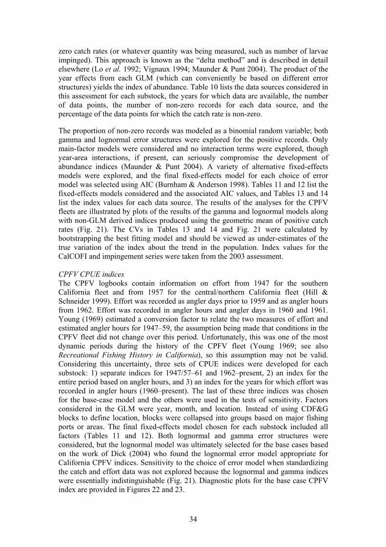
zero catch rates (or whatever quantity was being measured, such as number of larvae impinged). This approach is known as the “delta method” and is described in detail elsewhere (Lo et al. 1992; Vignaux 1994; Maunder & Punt 2004). The product of the year effects from each GLM (which can conveniently be based on different error structures) yields the index of abundance. Table 10 lists the data sources considered in this assessment for each substock, the years for which data are available, the number of data points, the number of non-zero records for each data source, and the percentage of the data points for which the catch rate is non-zero.

The proportion of non-zero records was modeled as a binomial random variable; both gamma and lognormal error structures were explored for the positive records. Only main-factor models were considered and no interaction terms were explored, though year-area interactions, if present, can seriously compromise the development of abundance indices (Maunder & Punt 2004). A variety of alternative fixed-effects models were explored, and the final fixed-effects model for each choice of error model was selected using AIC (Burnham & Anderson 1998). Tables 11 and 12 list the fixed-effects models considered and the associated AIC values, and Tables 13 and 14 list the index values for each data source. The results of the analyses for the CPFV fleets are illustrated by plots of the results of the gamma and lognormal models along with non-GLM derived indices produced using the geometric mean of positive catch rates (Fig. 21). The CVs in Tables 13 and 14 and Fig. 21 were calculated by bootstrapping the best fitting model and should be viewed as under-estimates of the true variation of the index about the trend in the population. Index values for the CalCOFI and impingement series were taken from the 2003 assessment. CPFV CPUE indices The CPFV logbooks contain information on effort from 1947 for the southern California fleet and from 1957 for the central/northern California fleet (Hill & Schneider 1999). Effort was recorded as angler days prior to 1959 and as angler hours from 1962. Effort was recorded in angler hours and angler days in 1960 and 1961. Young (1969) estimated a conversion factor to relate the two measures of effort and estimated angler hours for 1947–59, the assumption being made that conditions in the CPFV fleet did not change over this period. Unfortunately, this was one of the most dynamic periods during the history of the CPFV fleet (Young 1969; see also Recreational Fishing History in California), so this assumption may not be valid. Considering this uncertainty, three sets of CPUE indices were developed for each substock: 1) separate indices for 1947/57–61 and 1962–present, 2) an index for the entire period based on angler hours, and 3) an index for the years for which effort was recorded in angler hours (1960–present). The last of these three indices was chosen for the base-case model and the others were used in the tests of sensitivity. Factors considered in the GLM were year, month, and location. Instead of using CDF&G blocks to define location, blocks were collapsed into groups based on major fishing ports or areas. The final fixed-effects model chosen for each substock included all factors (Tables 11 and 12). Both lognormal and gamma error structures were considered, but the lognormal model was ultimately selected for the base cases based on the work of Dick (2004) who found the lognormal error model appropriate for California CPFV indices. Sensitivity to the choice of error model when standardizing the catch and effort data was not explored because the lognormal and gamma indices were essentially indistinguishable (Fig. 21). Diagnostic plots for the base case CPFV index are provided in Figures 22 and 23.

34

The spatial nature of catch rates along the California coast was explored in two ways. First, the percent index of relative importance (%IRI; Pinkas et al. 1971; Cortez 1999) – using numbers of cabezon, weight of cabezon catch, and frequency of cabezon occurrence – was used to summarize the contribution of each location (Fig. 24) and blocks within location (Fig. 25) to the CPFV fishery. For the NCS, Halfmoon Bay and Morro Bay comprised over two-thirds of the total IRI (Fig. 24). In both of these complexes, multiple blocks contributed to the total location IRI (Fig. 25). In the south, most of the IRI is contributed by the northern-most locations (Fig. 24) and no one block dominated the catch. Second, CPUE indices were developed for each location to compare trends on smaller spatial scales (Figs. 26 and 27). Trends varied among locations within substocks indicating potentially different patterns in abundance through time. In general, the most distinctive declines were found in the southern locations of the NCS and in more recent years throughout the SCS. An index from the central California CPFV observer program (1987–98), operated by CDF&G, was also considered during the 2003 assessment. The CPFV logbook and CPFV observer series exhibit similar trends (Cope et al. 2004). The index developed from the observer data was not used in this assessment because the observer program information is not independent from the information contained in the CPFV logbooks and the indices based on the logbook data represent the longer time series. Adult Surveys Two fishery-independent surveys were investigated for potential use in the NCS assessment (Table 10). The first is a visual count of adult fish among nearshore rocky reefs in the Monterey area during 1993–98 (the “Monterey adult survey”). Transects were either randomly assigned or repeated on permanent transects. Lengths of transects varied from a few minutes to over an hour. All cabezon were counted and assigned to different life history categories (YOY, juvenile, subadult, and adult). Adults were used to develop an abundance index using year, month, location (reef) and depth as factors (Table 11).

The second fishery-independent survey was a nearshore benthic survey of adult fishes, conducted from 1977–2002 by TENERA Environmental (an environmental consulting firm in San Luis Obispo, CA) at one site just south of Point Buchon (Figure 1). Transects were 50m in length in depths from 3–10 m along high to moderate relief rocky reefs and kelp forests. Abundance indices were developed using the factors year and month (Table 11).

These two indices were not included in the NCS base case model for two reasons: 1) SCUBA surveys may not provide reliable abundance indices for cryptic species such as cabezon; and 2) the spatial coverage of these surveys, which is limited, is such that abundance indices based on them may not be representative of coastwide trends. To explore the second issue, the standardized abundance estimate from the TENERA survey was compared to its nearest fishing location, Morro Bay (Fig. 26). The trends are quite different, supporting the conclusion that the TENERA data is not appropriate to include in the current assessment base case model. Despite not including either of these adult surveys in the base case, sensitivity of the results of the assessment to their inclusion is examined.

35

CalCOFI The Southwest Fishery Science Center (SWFSC) has conducted larval tows off California since 1950. Tows are generally made at stations from the Mexican border to roughly 36°N, so these data relate primarily to southern California. Surface (manta) and subsurface (oblique) tows are taken, but the subsurface tows catch few cabezon (Table 10) and are therefore not considered further in this assessment. Surface tows made south of 31°N during June-September and west of 122°W are also excluded from the analyses due to few positive tows. Additionally, data for the years 1977, 1979, 1982 and 1983 are excluded because of changes in survey methodology. The factors considered in the analyses were: day and night (day: between 6AM and 6PM), latitude (north and south of 34°N), longitude (east and west of 121°W), and month. The resultant index is shown in Figure 28. Power-plant Impingement An index of recruitment was created using impingement data obtained from the Edison power plants in California (Figure 29). These data (catch in numbers per standardized flow volume) come from only the extreme southern California Bight (33-34°N) and are consequently used only for the assessment of the SCS. The factors considered when developing this index were: station (some stations had multiple intake areas), and season (Dec-Feb, Mar-May, Jun-Aug, and Sept-Nov). This index is considered to pertain to recruitment rather than to reproductive output because the lengths of the fish impinged were primarily those of fish aged 0 and 1 years (Figure 30).

Ichthyoplankton Indices Cabezon larvae are initially neustonic and available (and readily identifiable) to planktonic sampling gears. The SWFSC has conducted ichthyoplankton surveys off the west coast and developed databases with information on the abundance of cabezon larvae. Generally the size of fish collected during these studies is <15mm (pre-settlement) and therefore not thought to correlate well with recruitment to age-1. However, the abundance of this size group may relate (in a linearly proportional way) to the amount of reproductive output the year before the year of sampling. The possibility of developing an index using the Santa Cruz mid-water juvenile rockfish survey was investigated. However, cabezon are only a very small component of the catch in this survey (Steve Ralston, SWFSC, pers. comm.) so no attempt was made to develop an index of pre-settlement cabezon using these data. RecFIN The 2003 assessment considered a recreational CPUE index based on data for the shore and PBR fleets combined. An index of abundance based on CPUE data would be required separately for each fleet for this assessment because it considers each of these modes separately. The catch and effort data for the PBR fleet was explored and it was found that there are few records with cabezon (Table 10). An abundance index based on RecFIN is therefore not considered further in this assessment.

Southern California Sanitation Districts Fish Surveys The sanitation districts of Los Angeles, Orange, and San Diego Counties and the City of Los Angeles conduct fish surveys every year to monitor the effects of sewage outfall on nearshore communities. As was the case with the size composition data,

36

none of these data sources provided sufficient information to develop indices of abundance for cabezon. Data Input Files The SS2 input files for each substock are provided in Appendices B-1 (NCS) and C-1 (SCS). Assessment Assessment Model This is the second assessment of the cabezon resource off the California coast. It differs in several key ways from the past assessment (Cope et al. 2004). The past assessment was based on an age- and sex-structured population dynamics model developed specifically for cabezon in AD Model Builder (Otter Research Ltd.). In contrast, the present assessment is based on Stock Synthesis 2 (SS2; Methot 2005), a flexible length- and age-based population dynamics modeling environment. The two models differ in terms of how the recruitment bias-correction is modeled, whether the impact of selectivity on weight-at-age is accounted for, and whether additional survey index variability is estimated. A formal comparison of the two models is provided in Appendix D.

Another major difference from the past assessment is that California is divided into two regions for the purposes of this assessment. The ecology of nearshore reef fishes leads to the expectation of low rates of movement among reefs. This, combined with the different fishing histories of central/northern California and southern California, imply different time-trajectories of population size in these two broad regions. Although even finer scale assessments would be desirable (e.g. by conducting assessments separately for northern and central California), the two-substock approach is the only one that can be supported by the currently available data. Results from a one-stock model with twelve fleets representing the area-specific fleet designations of the two-substock model are also presented for comparison. This model includes all of the indices used in the assessments of the NCS and the SCS.

The population dynamics model The base case assessment for each substock is based on the following assumptions:

1. There are two fishery sectors (commercial and recreational). The commercial sector consists of two fleets and the recreational sector consists of four fleets.

• Fleet 1: Commercial non-live-fish fishery • Fleet 2: Commercial live-fish fishery • Fleet 3: Recreational mode: Man-made • Fleet 4: Recreational mode: Shore • Fleet 5: Recreational mode: Private boat and rentals (PBR) • Fleet 6: Recreational mode: Commercial Passenger Fishing Vessel

(CPFV). Fleet distinctions imply different length-specific selectivity patterns.

2. Selectivity is assumed to be dome-shaped for the commercial live-fish fishery and the man-made and shore fleets in the recreational fishery because each of these fleets tends not to land the larger sized fishes. Selectivity is assumed to be asymptotic and related to length by a logistic function for the remaining

37

fleets. All selectivities are assumed to be constant over time. The sensitivity of the results of the assessment to alternative specifications related to selectivity is examined in the tests of sensitivity. The selectivity patterns for the commercial fleets in the assessment of the SCS are set to those for the commercial fleets in the NCS owing to a lack of size composition data for the commercial fleets in the SCS.

3. There is one fishing season each year and the removals are taken instantaneously in the middle of the year after half of the natural mortality.

4. The estimates of removals-in-mass are known with negligible error. 5. Recruitment is related to reproductive output by means of a Beverton-Holt

stock-recruitment relationship with log-normally distributed process error. 6. Length-at-age is normally distributed about its expected value. 7. There is no connection between the two substocks of cabezon, either through

recruitment or migration.

Parameter estimation The population dynamics model includes many parameters. The values for some of these parameters are based on auxiliary information, while others are estimated by fitting the model to the data (Table 15). The base-case value for steepness (h) is assumed to be 0.7 based on a recommendation from the past assessment. The implications of this choice of steepness is evaluated using a likelihood profile. Recruitment variation, , is set equal to 1.0 as was case for the past assessment. The base-case values for the instantaneous rate of natural mortality are set to 0.25yr-1 for females and 0.3yr-1 for males (Table 2). Given the considerable uncertainty associated with the (assumed) base-case values for and M, sensitivity tests examine the consequences of changing the values for these parameters.

Rσ

Rσ

Growth is not estimated within the model. Rather, the values for the parameters related to growth and fecundity are taken from Table 1. The values that determine the variability in length-at-age are computed by assuming that the coefficient of variation of the length at age 1 is 0.14 and that at age 17 is 0.09. There is an indication that the CV of length-at-age decreases linearly with age for many marine fishes (Erzini 1994). The only data on length-at-age for cabezon (Grebel 2003; Fig. 3A) indicates that the coefficient of variation for age-0 females is 0.11 and that for age-0 males is 0.14, while the coefficient of variation of length-at-age for age-10 is 0.01 for females and 0.09 for males. These values were based on small sample sizes (2 to 13 animals), therefore the upper limit for the CVs (0.14 and 0.09) are assumed for the base-case analyses and the value for age 10 is increased slightly and assumed to apply to age 17.

No attempt is made to estimate recruitment deviations for the first year of the assessment period (1916), nor those for some of the subsequent years, because the data are completely uninformative regarding the values for some of the early (and most recent) recruitment deviations. Running the NCS model while estimating all recruitments produces a recruitment event in 1960 almost three times larger than any another recruitment event, while doing the same in SCS, produces a relatively poor recruitment history (Fig. 31). The past assessment considered the availability of length-composition and impingement data to determine the years for which recruitment deviations should be estimated. For this assessment, the base-case models for each substock were run estimating recruitment deviations for all years to determine the first year for which recruitment deviations could be estimated with

38

reasonable precision. The asymptotic standard deviations for the recruitment deviations are shown in Fig. 32. A decrease in these standard deviations may indicate when estimation of recruitment deviations should begin because the data provide some information about the recruitment deviations. There is a dramatic drop in the asymptotic standard deviation of the recruitment deviations for the SCS in 1970, but only a slow and steady decline in these asymptotic standard deviations for the NCS after 1960. Considering all of these factors, 1970 was chosen as the first year for which a recruitment deviation is estimated for the SCS and 1980 for the NCS (the latter based mostly on available length data). The base case models end recruitment estimation in 2003 because there is no information available to estimate a 2004 value, though the choice of the last year for which a recruitment deviation is estimated may impact the results of the assessment (Fig. 33). Therefore, sensitivity of the assessment results to the years for which recruitment deviations are estimated is considered in the tests of sensitivity.

Selectivity as a function of length was estimated for all fleets for which mean weight or length-composition data were available. Dome-shaped selectivity was modeled using an eight-parameter double-logistic curve for the commercial live-fish and recreational man-made and shore fleets. All parameters were estimated except for the minimum size selectivity (parameter 2) and the width of the dome (parameter 8) for the live-fish and shore fleets. For the man-made fleet, the initial slope (parameter 4) and the selectivity at the maximum size (parameter 5) were also pre-specified (Table 15). Length selectivities for the non-live commercial and recreational PBR and CPFV fleets were described using a logistic equation with both parameters estimated. There are no length-frequency data for the commercial fleets for the SCS, so the selectivity patterns for these fleets were set to those estimated for the NCS. The selectivity pattern for the CPFV fleet used when calculating the model-estimates for the indices of abundance derived using the catch and effort data for the CPFV fleet were set to those for the CPFV fleet. Age selectivities with full selectivity at age 0 and age 0 to 1 only were assumed when fitting to the CalCOFI larval tows and power plant impingement data, respectively. Sensitivity to alternative formulations of the CalCOFI larval survey selectivity was explored by parameterizing to fully select age 5 and older individuals and matching the selectivity to the maturity function.

Likelihood components The following five components comprised the objective function that was minimized to estimate the free parameters of the model:

1. Abundance Index (assumed to be log-normally distributed). 2. Mean Weight (assumed to be normally distributed). 3. Length Composition (assumed to multinomially distributed). 4. Recruitment Deviations. 5. Parameter Priors (penalties on deviations from the prior distribution;

generally very small for these model parameterizations)

Coefficients of variation about the abundance indices derived from bootstrapping or jackknifing techniques may greatly underestimate the true uncertainty regarding the relationship between these indices and biomass. A catchability scaling parameter was estimated during the 2003 assessment to inflate the coefficients of variation for the indices. That option is not currently available in SS2, so the pre-specified coefficients of variation for the abundance indices were adjusted iteratively until the model-

39

calculated R.M.S.E. matched the pre-specified coefficient of variation for each index. The sensitivity of the results to setting the coefficients of variation to those obtained from the bootstrap procedure (Tables 13 and 14) is explored in the tests of sensitivity.

The mean weight data (Table 9) were assumed to be normally distributed with coefficients of variation based on the raw data when these data were included in the objective function. The coefficients of variation for the estimates of mean weight for the CPFV fleet for 1947–51 for the NCS were set to 0.5 (larger than observed for RecFIN – average CV = 0.41) to avoid over-weighting these early data.

The catch length-composition data were pooled into 44 length-classes, each of width 2cm (first length-class 0–7.9cm). Although the length compositions can be based on hundreds or thousands of measurements, fits to length-frequency data usually exhibit substantial overdispersion relative to a multinomial distribution where the sample sizes are set to the number of animals measured. Therefore, for the purposes of the present analyses, the sample sizes are compared to the “effective” number of animals measured each year using the approach developed by McAllister and Ianelli (1997). Sample sizes are then iteratively changed to the effective sample sizes until the mean inputted sample sizes are similar to the mean effective sample sizes. Alternatively, one could set an upper limit to the effective sample size (say 200) to avoid large differences in sample sizes across fleets. For instance, the fleet with the largest average sample size would receive a maximum value 200 for all sampled years. The average sample sizes for all other fleets could then be re-scaled in relation to 200 based on their relationship to the fleet with the highest average sample size. Finally, the iterative procedure would be followed to obtain the final effective sample sizes internally consistent with the model, with the maximum value possible being 200. Model sensitivity to the method used to assign effective sample sizes and to assuming the original sample sizes (Table 8) was explored in the tests of sensitivity.

Recruitment deviation and parameter priors were calculated assuming lognormal and normal error structures, respectively. The variances for all of the estimated parameters were set very high to minimize the influence of the prior on the results.

Parameter (Control) Input Files The SS2 files for the assessments of each substock are provided in Appendices B-2 (NCS) and C-2 (SCS).

Model diagnostics (base models) Abundance Surveys Figures 34 and 35 show the fits to the base-case indices of abundance for the NCS and SCS respectively. As expected from the 2003 assessment, the model tracks the changes in the CPFV indices qualitatively, but there are considerable differences between the model-estimates and the data for some years. These differences are consistent with the very wide confidence intervals assumed for the data. The fit of the CPFV index for the SCS (Fig. 35) is particularly poor in the most recent years. This is because the length and weight data drive population dynamics rather than the abundance index information, with the result that the model predictions are substantially in excess of the observations. The NCS model also tends to overestimate the index values in more recent (post-1990) years (Fig. 34). The CalCOFI and Impingement indices are imprecise, and the fits to these data series are also not very good, particularly that to the CalCOFI index in recent years (Fig. 35).

40

Mean Weights Figures 36 and 37 show the fits to the mean weight data by substock. The confidence intervals for the mean weights are wide (as expected given the CVs in Table 8), which implies that the model is not constrained to a substantial extent by these data, particularly for the NCS. The fit of the model to the data for the PBR mode (fleet 5) for the NCS is very poor with the model consistently over-estimating the mean weight of the catch. Given that the model is able to mimic the length-frequency data for this fleet, this suggests a conflict between the length and weight data, undersampling of the weight data, or error in the length-weight relationship (or both). There are no very poor fits to the mean weight data for the SCS (Figure 36), although there remain runs of residuals for some fleets. The 95% confidence intervals for some of the mean weights are quite narrow for the SCS and the model consequently attempts to mimic these mean weights quite closely. One reason for the increasing trend in abundance evident for the SCS is the low mean weight for the man-made fleet (fleet 3) in 2000. This weight is interpreted as a recruitment event, which translates into large increases in biomass during the final years of the assessment period. Sensitivity to the inclusion in the assessment of this data point is explored below. Length-composition Data The base-case fits to the length-composition data for the NCS are given in Figures 38–43 and the corresponding Pearson residuals are summarized in Figures 44 and 45. Note that fits for the shore and man-made fleets are not shown because the lengths for these fleets are derived from weights (Table 7). When interpreting these figures, it should be noted that the observed and model-predicted lengths are “plussed” at low and high sizes. This has little impact on the results at high size, but can give a misleading impression at low size (e.g. the fit to the data for 1999 and 2000 for the non-live-fish fleet (Figure 38)). The fits to the length frequency data for the commercial fleets (Figures 38 and 39) are better than those to the data for the recreational fleets (Figures 40–43) and consequently have the higher effective sample sizes. Of the recreational fleets, the fits to the observer data for the CPFV fleet (Figure 42) are better than those to the data for the remaining fleets. This result is hardly surprising given the actual sample sizes for the various recreational fleets (Table 8). The fits to the length-composition data for the SCS (Figures 46 and 47) and the corresponding Pearson residuals (Figure 48) are only shown for two of the six fleets as there are either no length data or the length data are all computed from measured weights for the remaining fleets. As before, the fits to the CPFV observer data are better than the fits to the recreational PBR data.

Results Base-case results: NCS Figure 49 shows the MPD estimates of the time-trajectories of reproductive output (in absolute terms) and recruitment, along with their asymptotic 95% confidence intervals. There is considerable inter-annual variation in recruitment. The estimates of recruitment are most precise before 1980 and recently, because no recruitment deviations are estimated for these years and the estimates of recruitment consequently reflect expectations based on the stock-recruitment relationship (Figure 49B). In contrast, the estimates of reproductive output are most precise during the late 1980s and early 1990s (Figure 49A). The NCS is estimated to have been at 40.1% of its virgin level at the start of 2005 (445 mt). Major recruitment events are seen in the

41

1990s. Figure 50A shows the estimated spawner-recruit relationship. Appendix E lists the MPD estimates of the numbers-at-age matrix for each gender.

Figures 51 and 52 show the length- and age-specific selectivity ogives for each fleet. The live-fish fishery (fleet 2) is dome-shaped with respect to length. Selectivity for the man-made and shore fleets (fleets 3 and 4) also decline with size. Males are less selected than females for a given age because females are larger at age. Selectivity based on age and length suggests that immature fish are not completely excluded from the current and historical catch, especially in the man-made and shore fisheries.

Harvest rates for each fleet are given in Figure 53. The onset of the live-fish fishery in the late 1990s is dramatic and the peak harvest rate by this fleet is greater than that for any other fleet. The PBR harvest rates during the 1980s also represent a major period of removals from NCS. Base-case results: SCS Figure 54 shows the MPD estimates of the time-trajectories of reproductive output (in absolute terms) and recruitment, along with their asymptotic standard errors. The time-trajectory of reproductive output drops dramatically after 1980, stays low until the early 2000s, and then increases substantially. The increase in reproductive output occurs because of the 2000 year-class, the largest in the time-series. The size of this year-class is inferred primarily from the mean weight data for 2000 for the man-made recreational fleet (fleet 3). The major recruitment events are consistently lagged 1 year compared to the NCS. The reproductive output is estimated very precisely during the 1990s. The SCS is estimated to have been at 28.3% of its virgin level at the start of 2005 (71 mt). The biomass of cabezon off southern California is smaller than that off central / northern California and the resource is estimated to be more depleted off southern California than off central/northern California. Figure 50B shows the estimated spawner-recruit relationship. Appendix F lists the MPD estimates of the numbers-at-age matrix.

Figures 55 and 56 show the length- and age-specific selectivity ogives for each fleet. The selectivity patterns for the non-live-fish and live-fish fleets are set to those for the NCS. The selectivity patterns for the man-made and shore fleets decline more rapidly with length for the SCS than is the case for the NCS. Males are less selected than females for a given age because females are larger at age and fish are generally caught smaller in the SCS relative to the NCS. Selectivity based on age and length suggests that immature fish are not completely excluded from the current and historical catch, especially in the man-made recreational fishery.

Harvest rates for each fleet are given in Figure 57. There are two significant periods of removals: 1) the 1980s when harvest rates increased dramatically because of the increase in recreational fishing, particularly by the PBR mode; and 2) the late 1980s when the live-fish fishery took large catches. The first of these periods of harvest, along with the lack of strong recruitment events, led to the large reduction in reproductive output during the early 80s (Fig. 54). Base-case results: One California stock Figures 58 and 59 show MPD estimates of the time-trajectories of reproductive output (in absolute terms) and recruitment, along with their asymptotic standard errors when the data for the NCS and SCS are combined, and cabezon off California are

42

consequently treated as a single homogenous population. Results are shown when all of the data are used and when the 2000 mean weight datum for the man-made fleet off southern California is ignored. The time-trajectory of reproductive output for the combined assessment is qualitatively similar to that for the SCS, although, as expected, biomass levels are higher. There is a large increase in reproductive output at the end of the time-series, which can be attributed to the 2000 mean weight datum for man-made fleet off southern California. The depletion of the combined resource is 50% at the start of 2005 (634 mt compared to an unfished spawning biomass of 1,268 mt).

Table 16 compares the estimates of the total California cabezon reproductive output from the two substock model, the one stock model, and the 2003 assessment model. Total reproductive output in 2003 is greater for both of the current models compared to the 2003 assessment. However, both 2003 depletion estimates from this assessment are within the uncertainty ranges presented in the 2003 assessment (Cope et al. 2004). The estimate of 2003 depletion from the one stock model is larger than that from the two substock model (Table 16). When the one stock model uses all of the length data reported in RecFIN (meaning all weights converted to lengths and true measured lengths), as was the case for the 2003 assessment, the estimate of the 2003 depletion is very similar to that obtained during the 2003 assessment (Table 16, “one stock/all lengths”).

Sensitivity analyses The sensitivity tests related to data set choices differed among substocks. The selectivity pattern for a fleet is fixed to that for the base-case analysis if removal of a data source causes selectivity for that fleet to be inestimable.

NCS Trial 1: Ignore the length composition data for the commercial non-

live-fish fleet (fleet 1). Trial 2: Ignore the length composition data for the commercial live-fish

fleet (fleet 2). Trial 3: Ignore the mean weight data for the recreational man-made

fleet (fleet 3). Trial 4: Ignore the length composition and mean weight data for the

recreational shore fleet (fleet 4). Trial 5: Ignore the length composition and mean weight data for the

recreational PBR fleet (fleet 5). Trial 6: Ignore the length composition and mean weight data for the

recreational CPFV fleet (fleet 6). Trial 7: Base the analysis on the CPFV index for 1957–2003 (Table

13). Trial 8: Base the analysis on the CPFV indices for 1957–61 and 1962–

2003 (Table 13). Trial 9: Do not include the CPFV index Trial 10: Add the Monterey adult survey and the TENERA adult survey. Trial 11: Add the TENERA adult survey. Trial 12: Add the Monterey adult survey. Trial 13: Nonlinear relationship between CPUE and abundance (β = 0.5).

43

SCS Trial 1: Ignore the mean weight data for the recreational man-made

fleet (fleet 3). Trial 2: Ignore the mean weight data for the recreational shore fleet

(fleet 4). Trial 3: Ignore the all mean weight data for the recreational shore fleet

except the data point for 2000. Trial 4: Ignore the length composition and mean weight data for the

recreational PBR fleet (fleet 5). Trial 5: Ignore the length composition and mean weight data for the

recreational CPFV fleet (fleet 6). Trial 6: Base the analysis on the CPFV index for 1947–2003 (Table

13). Trial 7: Base the analysis on the CPFV indices for 1947–61 and 1962–

2003 (Table 13). Trial 8: Ignore all CPFV indices. Trial 9: Ignore the CalCOFI index. Trial 10: Ignore the Impingement index. Trial 11: Use the CPFV index only. Trial 12: Nonlinear relationship between CPUE and abundance (β = 0.5)

The results of these sensitivity analyses are provided in Table 17. Table 18 examines the sensitivity of the results to changing the values for M and Rσ , and Table 19 explores the sensitivity of the results to: a) the years for which recruitment residuals are estimated, b) the specifications for length-/age-specific selectivity, c) the specifications of the CalCOFI selectivity, d) the length data included in the analyses, e) the coefficients of variation assumed for the abundance indices, f) the effective sample sizes assumed for the length-composition data, g) the historical catches, and h) the coefficients of variation assumed for length-at-age.

Overall, the results in Tables 17 indicate that the NCS model is not greatly sensitive to adding or removing data sources. Ignoring the length-composition data for the live-fish commercial fleet (trial 2), ignoring the size information for the recreational man-made and shore fleets (trials 3 and 4), including the longest CPFV time-series (trial 7), and excluding all CPFV indices (trial 9) all lead to less optimistic estimates of depletion. Ignoring the size information for the CPFV fleet (trial 6) leads to more optimistic estimates of depletion. The results are most sensitive to including the TENERA adult survey (trials 10 and 11). The inclusion of this index leads to markedly lower estimates of current depletion, though the fits to the TENERA index are not good (Fig. 60). The potential to miss cryptic species using SCUBA surveys, and the inconsistency between the CPFV index for Morro Bay and the TENERA index (Fig. 26) suggests that the limited spatial coverage of the TENERA survey is such that this index does not provide an index of abundance for the entire NCS. This finding should not, however, rule out future use of other spatially-limited fishery-independent surveys.

The SCS model is also generally insensitive to the data sources included in the assessment (Table 17), except for one important case; the exclusion of the man-made mean weight data (trial 1). Exclusion of these data leads to the conclusion that stock is much more depleted than is suggested by the base-case analysis. Figure 61 compares

44

the estimated time-trajectory of reproductive output (upper panel) and recruitment (lower panel) with and without the mean weight data for the man-made fleet for 2000. The estimates of recruitment are similar up to 2000, when the analysis that ignored the 2002 mean weight datum suggests complete recruitment failure. Figure 62 compares the fits to the length-composition data for PBR fleet when the mean weight datum in year 2000 for this fleet is (base case) or is not included in the analysis. The fit to the length-composition data for 2002 is slightly better when this data point is ignored, but the fit to the length-composition data for 2003 data is better when this data point is not ignored. There is also a noticeable cohort in the data for years 2002-2004 of correct length to support a recruitment event in year 2000. These results, along with evidence for strong year-classes in 1999 or 2000 for several others species off the California coast, suggests that there may have been a strong year-class in 2000 and consequently that the 2000 mean weight datum for the man-made fleet should not be ignored.

The results in Table 18 indicate that the assessments for both substocks are more sensitive to the values assumed for M than to that assumed for Rσ , and more sensitive to the value for female M than to that for male M. Decreasing female M from its base-case value leads to a more depleted resource and vice versa. Both substocks are estimated to be more depleted as is increased. The fit of the model to the data, as quantified by the value for the negative-log-likelihood, improves as M is increased.

Rσ

The factors considered in Table 19 generally had less impact on the outcomes from the assessment than those examined in Tables 17 and 18. The factors that changed the depletion for the NCS the most were starting recruitment estimation before 1970 or in 1990, the use of RecFIN weights as lengths (“all lengths”), and the values assumed for variation in length-at-age. Specifically, the results for NCS are sensitive to the assumption that length-at-age CVs change linearly and decrease with age, although this assumption seems biologically realistic The results for the SCS were most sensitive to the years for which recruitment residuals are estimated (mainly pre-1970 and 2004), making the selectivity patterns for all fleets logistic, halving catches, and the assumed level of variation in length-at-age. These sensitivities lead to less optimistic appraisals of stock status, including that the stock may be depleted to below 25% of its unfished level at present. The estimates of absolute spawning biomass are more sensitive than those of depletion. Figure 63 shows substock-specific likelihood profiles for steepness and Figure 64 provides the subsequent estimates of unfished spawning and current biomass and current depletion. The data argue for a steepness of 1 for the SCS, but this may be more indicative of the data being uninformative. Local minima are also apparent within these profiles, though they seem not to affect the results greatly. Projection and decision analysis Twelve-year yield forward projections are conducted for each substock under two alternative ABC control rules (based on FMSY proxies of F45% and F50%) and two OY threshold control rules (40-10 or 60-20). The standard PFMC OY control rule for groundfish such as cabezon is based on F45% with a 40-10 adjustment for stocks below the target level of 40% of the unfished reproductive output. The California Nearshore Fishery Management Plan proposes the use of a FMSY proxy of F50% and a 60-20 adjustment for stocks below 60% of the unfished reproductive output. The relative

45

proportion of the six fleets in future harvests is assumed to be the same as the last year (2004) in the model. The results in Table 20 suggest that a reduction in population size will occur for the NCS under the two control rules based only on the FMSY proxies. In contrast, the projections for the remaining control rules suggest that some increase in reproductive output will occur. The extent of this increase is greatest for the most conservative OY control rule (F50% with a 60-20 adjustment) and least for the least conservative control rule (F45% with a 40-10 adjustment). The projections for the SCS model beyond 2006–07 should be interpreted with considerable caution because they are influenced by the (strong, but uncertain) 2000 year-class. Projections based on alternative states of nature for each substock were explored to capture uncertainty in population conditions. For the NCS, the low and high M scenarios refer to different assumptions about sex-specific natural mortality and were selected to represent the 95% confidence intervals for terminal spawning biomass based on the Hessian approximation. The low scenario assumes M = 0.2yr-1 and 0.25 yr-1 for females and males respectively, while the high scenario assumes 0.3 yr-1 and 0.35 yr-1 respectively. For the SCS, the low and high depletion rates refer to depletion rates in 2005 of roughly 20% and 35%, respectively.This range of depletion for the SCS was determined by the STAR panel to adequately cover uncertainty in its value and was determined by modifying the year 2000 man-made fleet mean weight CV value (e.g. an increase in the CV lead to a less depleted resource in 2000). These states of nature attempt to capture the uncertainty in current depletion based on the uncertainty in the magnitude of the 2000 recruitment. Probabilities for each state of nature were calculated, as directed by the STAR panel, assuming a normal probability density function (pdf) parameterized by the expected base case depletion rate and its asymptotic standard deviation.These respective substock pdfs were used to estimate the cumulative densities at the low and high depletion rates of 0.3 and 0.49 for the NCS and 0.2 and 0.35 for the SCS. Each cumulative density, representing the mid-point of the total density of each state of nature, was then doubled to determine the associated probability for each state of nature. Results from each of the states of nature are given in Figure 65. Decision analysis population projections are provided in Table 21 for each state of nature and several state-dependent future catch series. The NCS will drop below the overfished level if catch levels are based on the 40-10 rule and the high M scenario, but the true state of nature is either the base case or low M scenario. This also occurs if catches are based on the base case model but the low M state of nature is correct. All other scenarios lead to depletion levels above 25% in 2016. Under the 60-20 rule, only the high M catch with a low M true state of nature leads to a depletion level in 2016 below 25%. In the SCS, all combinations of catch and true state of nature under either control rule lead to a depletion level in 2016 larger than 25%. Response To STAR Panel Review The STAR panel, during its review of the assessment, made several recommendations for further model exploration. The following is a list of these recommendations and the subsequent STAT team responses:

46

1. SCS Fleet 3 year 2000 mean weight datum: The STAR panel recommended further exploration of the effects of the mean weight datum for the SCS for 2000. This request was met and lead to examination of model fits with and without the mean weight datum for 2000, specifically to the length-composition data for the PBR fleet (the only fleet with length fits post-1999). Fits with and without the mean weight datum for the PBR fleet in 2000 are included in Figure 62 and lead to greater confidence in the existence of a large 2000 year-class in the SCS. 2. TENERA adult survey: The NCS model was sensitive to the exclusion of the TENERA adult survey so the STAR panel requested to see the model fits when this survey was included. This request was met and model fits with and without the TENERA adult survey are shown in Figure 60. The STAR panel also suggested comparing the trend in abundance indicated by the TENERA survey to the CPFV CPUE trend for Morro Bay. This request was met (Figure 26). 3. Effective sample sizes: The STAR panel expressed concerns over the method used to determine the effective samples sizes for the length-composition data. Specifically, there were orders of magnitude differences in effective samples sizes among years within some fleets. An alternate method of calculating effective samples sizes was defined. This request was met by an additional sensitivity run for each substock (Table 19) that found no notable differences in model outputs between the two methods for calculating effective sample sizes. 4. Local minima in the steepness profiles: The STAR panel felt that the likelihood profiles for steepness needed additional work to address the lack of smoothness and suggested finer increments when calculating these profiles. This request was met, but the profiles remained clunky (Figs. 62 and 63), suggesting local minima. 5. One sex model: The STAR panel suggested the exploratory development of a one-sex model because the nest-guarding behavior of males should increase their contribution to future reproductive output and thus their value in the population dynamics. This request was met and a one-sex model was produced, but it ultimately just combined the male and female spawning biomasses. It did highlight, however, the issue of what population metric, instead of spawning biomass, should be used when males contribute more than just sperm to reproductive output. 6. Location-specific CPUE analysis: In addition to the IRI spatial catch analysis, the STAR panel suggested the STAT team produce CPUE trends for each location within a substock and compare trends among areas. This analysis was completed and its results are presented in Figs 26 and 27. Research Recommendations 1. Accurate accounting of removals, especially from the recreational and live-fish fisheries: Fisheries primarily exploited by recreational and live-fish commercial fisheries are traditionally hard to monitor. More effort to monitor these fishery sectors may be necessary to accurately monitor fishing mortality.

47

2. A fishery-independent survey of cabezon population abundance: The current fishery-independent survey being developed in the Morro Bay area will become an important input into future assessments of cabezon. Expansion of this survey will increase its usefulness as an index of abundance for central and northern California. 3. A study of the stock structure of cabezon: This assessment assumes two substocks of cabezon along the California coast. Current work on cabezon stock structure should be included in the next assessment. 4. Age validation/ age determination: Catch age-composition data were not available for this assessment. Accurate ageing is crucial to understand the population dynamics of a species, especially those for which there is limited survey information. Information on the age-structure of the catches for each fishery sector would substantially improve some aspects of the assessment. 5. A better understanding of the relationship between CPUE and population size: Changes in recreational CPUE indices are assumed to reflect changes in population size in a linearly proportional manner. The results of the assessment would be severely in error if this assumption were substantially violated. Therefore, if future assessments depend on CPUE data, it is vital that the relationship between CPUE and population size be quantified. 6. Alternative assessment procedures: The need for greater spatial resolution in the management of nearshore fisheries also increases the amount of data required to perform traditional stock assessments. Alternative assessment procedures that are less data-hungry, but still provide relevant management outputs should be developed to address this need. In addition, the nest-guarding behavior of males gives new value to males in the cabezon population. A metric other than spawning biomass may be needed to account for the male portion of the population in reference points. 7. Effect of climate on cabezon: Several of the data sources in this assessment (e.g. the power-plant impingement and CalCOFI indices, and some length-composition data) indicate that there was potentially good recruitment after 1999 (and before 1977 for the impingement data) whereas these same sources indicate that recruitment was very poor prior to 1999 in the SCS. Cabezon may be influenced by climatic/oceanic regimes. A better understanding of the relationship between cabezon population dynamics and climate would reduce the uncertainty of future assessments. 8. Sex-specific data: Given the strong correlation of color to gender in cabezon (O’Connell 1953; Lauth 1987; Grebel 2003), collection of sex-specific information (at least recording fish color) would greatly enhance future assessments.

48

References Alonzo, S.H., M. Key, T. Ish, and A.D. McCall. 2004. Status of the California

Sheephead (Semicossyphus pulcher) stock (2004). 146 p. Baxter, J.L. and P.H. Young. 1953. An evaluation of the marine sportfishing record

system in California. Calif. Fish and Game 39(3): 343-353. Best, E.A. 1963. The California marine fish catch for 1961/Catch localities for Dover

sole, Microstomus pacificus (Lockington), landed in California, 1950 through 1959. Fish Bull. 121. 56 p.

Burnham, K.P., and D.R. Anderson. 1998. Model selection and inference:. a practical information-theoretic approach. Springer-Verlag, New York,. NY. 353p.

Butler, J.L., L.D. Jacobson, J.T. Barnes, H.G. Moser, and R. Collins. 1999. Stock assessment of cowcod. In Pacific Fishery Management Council. Appendix: status of the Pacific coast groundfish fishery through 1998 and recommended biological catches for 1999: stock assessment and fishery evaluation. Pacific Fishery Management Council, Portland, Oregon.

CDF&G Bureau of Marine Fisheries Staff. 1949. Commercial fish catch of California for the year 1947 with an historical review 1916-1947. Fish Bull. 74. 272 p.

Calhoun, A.J. 1950. California angling catch records from postal card surveys: 1936-1948; with an evaluation of postal card response. Calif. Fish and Game 36(3): 177-234.

California Department of Fish and Game. 2002. Nearshore Fishery Management Plan. California Fish and Game Commission. 20 Lower Ragsdale Drive, Suite 100. Monterey, CA 93940.

Chen, S. and S. Watanabe. 1989. Age dependence of natural mortality coefficient in fish population dynamics. Nippon Suisan Gakkaishi 55: 205-208.

Classic, R.F. 1932. Fishing conditions, Monterey County. Calif. Fish and Game 18(3): 260-261.

Connor, G. 1937. Fish and game statistics. Calif. Fish and Game 23(2): 113-118. Cope, J.M., K.R. Piner, C.V. Minte-Vera, and A.E. Punt. 2004. Status and future

prospects for the cabezon (Scorpaenichthys marmoratus) as assessed in 2003. In Status of the Pacific coast Groundfish fishery through 2004. Stock assessment and fishery evaluation: stock assessments and rebuilding plans. Vol. I. Pacific Fishery Management Council, Portland, Oregon. Pacific Fishery Management Council, Portland, Oregon.

Cortes, E. 1999. Standardized diet compositions and trophic levels of sharks. ICES J. Mar. Sci. 56: 707-717.

Croaker, R.S. 1938. Let’s go fishing. Calif. Fish and Game 24(3): 280-287. Croaker, R.S. 1939. Three years of fisheries statistics on marine sport fishing in

California. Trans. Am. Fish. Soc. 69: 117-118. Dick, E.J. 2004. Beyond ‘lognormal versus gamma’: discriminating among error

distributions for generalized linear models. Fish. Res. 70: 351-366. Erzini, K. 1994. An empirical study of variability in length-at-age of marine fishes. J.

App. Ich. 10: 17-41. Feder, H.M., C.H. Turner, and C. Limbaugh. 1974. Observations on fishes associated

with kelp beds in southern California. Calif. Dept. Fish Game, Fish Bull. 160. 144 p.

Fry, D.H. 1932. Barge fishing, a southern California sport. Calif. Fish and Game 18(3); 244-249.

Garrison, K.J., and B.S. Miller. 1982. Review of the early life history of Puget Sound fishes. Contract 80-ABA-3360. NMFS, Seattle, WA, 729 p.

49

Grebel, J. 2003. Age, growth, and maturity of cabezon, Scorpaenichthys marmoratus, in California. Masters Thesis, Moss Landing Marine Laboratories/San Jose State University. 56 p.

Hill, K.H. and J.T. Barnes. 1998. Historical catch data from California’s commercial passenger fishing vessel fleet: Status and comparison of two sources. California Department of Fish and Game Marine Region Technical Report No. 60. 44 p.

Hill, K.H. and N. Schneider.1999. Historical logbook databases from California’s commercial passenger fishing vessel (partyboat) fishery, 1936-1997. SIO Reference Series No. 99-19.

Heimann, R.F. and J.G. Carlisle, Jr. 1970. The California marine fish catch for 1968 and historical review 1916-1968. Fish Bull. 149. 70 p.

Hoenig, J.M. 1983. Empirical use of longevity data to estimate mortality rates. Fish. Bull. 82: 898-902.

Holder, C.F. 1914. Attempts to protect the sea fisheries of southern California. Calif. Fish and Game 1(1): 9-19.

Jensen, A.L. 1996. Beverton and Holt life history invariants result from optimal trade-off of reproduction and survival. Can. J. Fish. Aquat. Sci. 53: 820-822.

Jordan, D.S. and B.W. Everman. 1898. The fishes of north and middle America. Part II. Bull. U.S. Nat. Mus. 47:1241-2183.

Karpov, K. A., D. P. Albin and W. H. V. Buskirk. 1995. The marine recreational fishery in northern and central California. Fish Bulletin 179.

Lauth, R.R. 1987. Spawning ecology and nesting behavior of the Cabezon, Scorpaenichthys mamoratus in Puget Sound, Washington. Masters Thesis. University of Washington. 104 p.

Lauth, R.R. 1988. Seasonal spawning cycle, spawning frequency and batch fecundity of the cabezon, Scorpaenichthys marmoratus, in Puget Sound, Washington. Fish Bull. 87: 145-154.

Lea, R. N., R. D. McAllister, and D. A. Ventresca. 1999. Biological aspects of nearshore rockfishes of the genus Sebastes from Central California. Fish Bull. 177.

Lo, N.C., L.D. Jacobson, J.L. Squire. 1992. Indices of relative abundance for fish spotter data based on delta-lognormal models. Can. J. Fish. Aquat. Sci. 49: 2515-2526.

Love, M.S., Axell, B., Morris, P., Collins, R., and Brooks, A. 1987. Life history and fishery of the California scorpionfish, Scorpaena guttata, within the Southern California Bight. Fish. Bull. 85: 90-116.

Love, M.S, L. Thorsteinson, C.W. Mecklenburg and T.A. Mecklenburg. 1996. A checklist of marine and estuarine fishes of the Northeast Pacific, from Alaska to Baja California. National Biological Service. Located at website http://id-www.ucsb.edu/lovelab/list.html.

Maunder, M.N. and A.E. Punt. 2004. Standardizing catch and effort data: a review of recent approaches. Fish. Res. 70: 141-159.

McAllister, M.K. and J.N. Ianelli 1997. Bayesian stock assessment using catch-age data and the sampling-importance resampling algorithm. Can. J. Fish. Aquatic Sci. 54: 284-300.

McCall, A. 2003. Status of bocaccio off California in 2003. In Status of the Pacific coast Groundfish fishery through 2003. Stock assessment and fishery evaluation. Vol. I. Pacific Fishery Management Council, Portland, Oregon. Pacific Fishery Management Council, Portland, Oregon.

50

Methot, R. 2005. User Manual for the Assessment Program Stock Synthesis 2 (SS2). Model Version 1.19. April. 47 p.

Methot, R., F. Wallace, and K. Piner. 2002 Stock status of the yelloweye rockfish resource in 2002. Appendix in Pacific Fishery Management Council. Status of the Pacific coast groundfish fishery through 2002 and recommended acceptable biological catches for 2003: stock assessment and fishery evaluation. Pacific Fishery Management Council, Portland, Oregon.

Miller, D.J. and D. Gotshall. 1965. Ocean sportfish catch and effort from Oregon to Point Arguello, California. Fish Bull. 130. 135 p.

Miller, D.J., and R.J. Lea. 1972. Guide to the coastal marine fishes of California. Dept Fish Game Fish Bull. 157, 249 p.

O’Connell, C.P. 1953. The life history of the cabezon Scorpaenichthys marmoratus. Fish Bull. 93. 76 p.

Oliphant, M.S., P.A. Gregory, B.J. Ingle, and R. Madrid. 1990. California marine fish landings for 1977-1986. Fish Bull. 173. 52 p.

Oregon Department of Fish and Wildlife. 2002. Interim Management Plan for Oregon’s Nearshore Commerical Fisherird. Oregon Department of Fish and Wildlife. 2040 SE Marine Science Drive. Newport, OR, 97365.

Pascual, M.A. and O.O. Iribarne. 1993. How good are empirical predictions of natural mortality? Fish. Res. 16: 17-24.

Pinkas, L., M.S. Oliphant, and C.W. Haugen. 1968. Southern California marine sportfishing survey: Private boats, 1964; Shoreline, 1965-1966. Fish Bull. 143. 42 p.

Pinkas, L., S. Oliphant, I.L.K. Inverson. 1971. Food habits of albacore, bluefin tuna and bonito in California waters. Fish Bull. 152: 1-105.

Pinkas, L., J.C. Thomas, J.A. Hanson. 1967. Marine sportfishing survey of southern California peirs and jetties, 1963. Calif. Fish and Game 53(2): 88-104.

Quast, J.C. 1968. New records of thirteen cottid and blennoid fishes for southeast Alaska. Pac. Sci. 22:482-487.

Ralston, S. and E.J. Dick. 2003. Status of black rockfish (Sebastes melanops) off Oregon and Northern California. In Status of the Pacific coast Groundfish fishery through 2003. Stock assessment and fishery evaluation. Vol. I. Pacific Fishery Management Council, Portland, Oregon. Pacific Fishery Management Council, Portland, Oregon. 75 p.

Scofield, N.B. 1928. Commerical Fishery Notes: Record catch recorded. Calif. Fish and Game 14(3): 249.

Starr, R.M., J.M. Cope and L.A. Kerr. 2002. Trends in Fisheries and Fishery Resources Associated with the Monterey Bay National Marine Sanctuary From 1981-2000. La Jolla, California, California Sea Grant College Program.

Vignaux, M. 1994. Catch per unit effort (CPUE) analysis of west coast South Island and Cook Strait spawning of hoki fisheries, 1987-1993. NZ Fisheries Association Research Document No. 94/11.

West Coast Groundfish Observer Program. 2005. West coast Groundfish observer program data report and summary analysis of non-sablefish endorsed limited entry fixed-gear permits. Northwest Fisheries Science Center. February. 11 p.

Young, P.H. 1969. The California Partyboat Fishery 1947-1967. Fish Bull. 145. 91 p.

51

Acknowledgements The STAT team would like to thank the following individuals for providing data or discussions useful to this assessment: Richard Charter SWFSC/CalCOFI), Meisha Key (CDF&G), Alec McCall (SWFSC), Don Pearson (SWFSC), Kevin Piner (SWFSC), Paulo Serpa (CDF&G), Deb Wilson-Vandenberg (CDF&G), and Dave VenTresca (CDF&G). Rick Methot (NWFSC) was especially helpful in answering any questions regarding SS2 and in exploring the OC/SS2 comparison. Ian Stewart (NWFSC) also provided advice using SS2 and in obtaining PacFIN data. The STAR panel (Steve Ralston (chair), John DeVore, Vivian Haist, Bob Mohn, Rod Moore, Paul Spencer, and Theresa Tsou) painstakingly evaluated the present work and provided invaluable recommendations on making the analysis more transparent. The data used in this assessment were collected by a great number of people that, although unknown and unnamed, have our appreciation.

52

Table 1. Biological parameters for cabezon. Values in parenthesis are the estimated standard errors. A. Age and growth (VBGF) parameters. Length in cm.

Parameter L∞ (cm) 95% C.I. k (yr-1) 95% C.I. t0 (yr) 95% C.I.

NCS Female 62.12 (3.53) 55.18 - 69.07 0.18 (0.03) 0.12 - 0.24 -1.06 (0.39) -1.82 - -0.29 Male 46.85 (2.50) 41.93 - 51.77 0.28 (0.07) 0.14 - 0.43 -1.19 (0.74) -2.53 - 0.26

Combined 56.78 (2.57) 51.73 - 61.83 0.20 (0.03) 0.14 - 0.26 -1.23 (0.38) -1.98 - -0.49

B. Relationship between maturity and age / length (combined sex and area) a b

age (years) -1.575 4.097 length (cm) -0.743 25.702

C. Weight (kg)-length (cm) relationship

a b R2 Sample Size NCS

Female 0.00000920 3.187 0.99 322 Male 0.00001163 3.118 0.96 227

SCS Female 0.00001236 3.113 0.95 55 Male 0.00001989 2.997 0.91 7

53

54

Table 2. Natural mortality calculations used to obtain sex-specific estimates of M used in the 2005 assessment. Method Equation Input values (per sex) Estimated M

Female Male Hoenig (1983) ln(Z) = 1.46 - 1.01ln(ω) ω = 17 (both sexes) -0.25 -0.25Chen and Watanabe (1989) k = 0.18 (F);0.28 (M) -0.20

a

-0.16 t0 = -1.06 (F); -1.18 (M)

Jensen (1996) M= 1.65/aM M = 7 (both sexes) -0.24 -0.24Jensen (1996) M= 1.5k k = 0.18 (F);0.28 (M) -0.27 -0.42Jensen (1996) M= 1.6k k = 0.18 (F);0.28 (M) -0.29 -0.45

Average M estimate -0.25 -0.30

0

0

0

0

0

( )

20 1 2

( )0

( )1

( )22

0

,1( )

,( ) ( )

1

0.51ln(1 )

M

M

M

Mk t t

MM M

k t t

k t t

k t t

ktM

k t teM t k t t

a a t t a t t

wherea e

a ke

a k e

t e tk

− −

− −

− −

− −

≤ −= ≥

+ − + −

= −

=

=−

=− − +

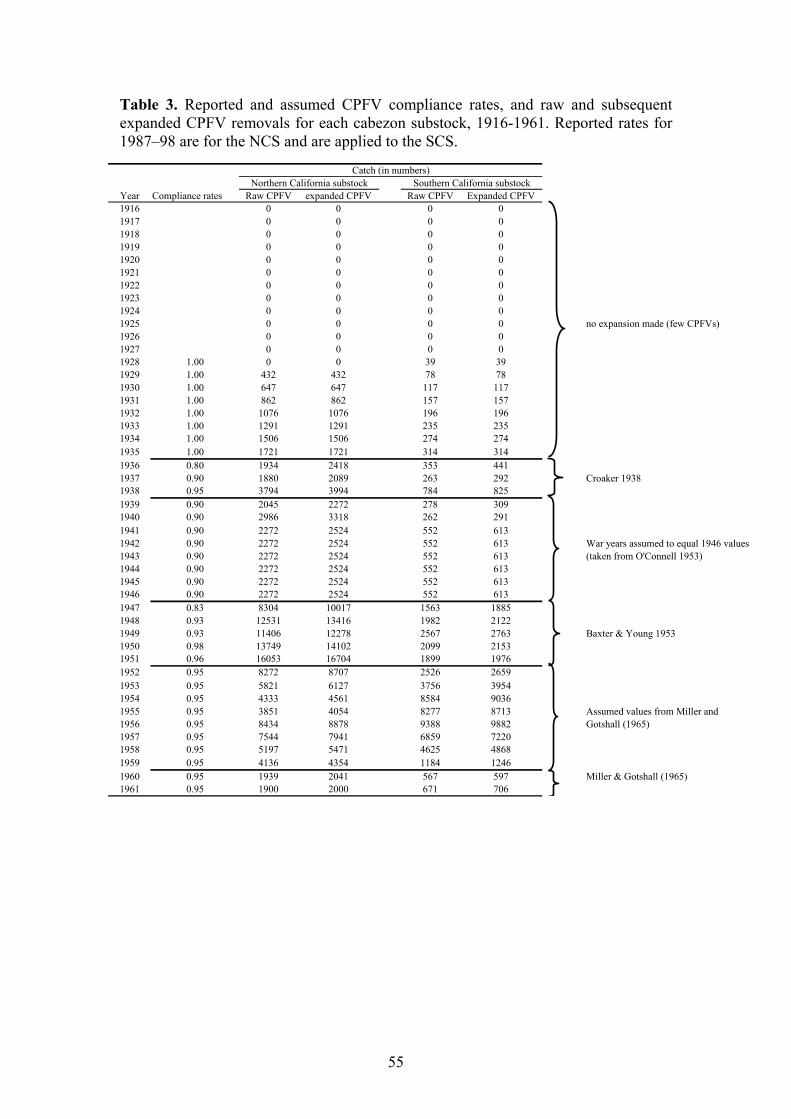
55

Year Compliance rates Raw CPFV expanded CPFV Raw CPFV Expanded CPFV1916 0 0 0 01917 0 0 0 01918 0 0 0 01919 0 0 0 01920 0 0 0 01921 0 0 0 01922 0 0 0 01923 0 0 0 01924 0 0 0 01925 0 0 0 0 no expansion made (few CPFVs)1926 0 0 0 01927 0 0 0 01928 1.00 0 0 39 391929 1.00 432 432 78 781930 1.00 647 647 117 1171931 1.00 862 862 157 1571932 1.00 1076 1076 196 1961933 1.00 1291 1291 235 2351934 1.00 1506 1506 274 2741935 1.00 1721 1721 314 3141936 0.80 1934 2418 353 4411937 0.90 1880 2089 263 292 Croaker 19381938 0.95 3794 3994 784 8251939 0.90 2045 2272 278 3091940 0.90 2986 3318 262 2911941 0.90 2272 2524 552 6131942 0.90 2272 2524 552 6131943 0.90 2272 2524 552 6131944 0.90 2272 2524 552 6131945 0.90 2272 2524 552 6131946 0.90 2272 2524 552 6131947 0.83 8304 10017 1563 18851948 0.93 12531 13416 1982 21221949 0.93 11406 12278 2567 2763 Baxter & Young 19531950 0.98 13749 14102 2099 21531951 0.96 16053 16704 1899 19761952 0.95 8272 8707 2526 26591953 0.95 5821 6127 3756 39541954 0.95 4333 4561 8584 90361955 0.95 3851 4054 8277 87131956 0.95 8434 8878 9388 98821957 0.951958 0.951959 0.951960 0.95 Miller & Gotshall (1965)1961 0.95

Northern California substock Southern California substockCatch (in numbers)

War years assumed to equal 1946 values (taken from O'Connell 1953)

Assumed values from Miller and Gotshall (1965)

Table 3. Reported and assumed CPFV compliance rates, and raw and subsequent expanded CPFV removals for each cabezon substock, 1916-1961. Reported rates for 1987–98 are for the NCS and are applied to the SCS.

7544 7941 6859 72205197 5471 4625 48684136 4354 1184 12461939 2041 567 5971900 2000 671 706

Table 3 (continued). Reported and assumed CPFV compliance rates, and raw and subsequent expanded CPFV removals for each cabezon substock, 1962-2004. Reported rates for 1987–98 are for the NCS and are applied to the SCS.

Year Compliance rates Raw CPFV expanded CPFV Raw CPFV Expanded CPFV1962 0.85 2663 3133 1845 21711963 0.85 5888 6927 3713 43681964 0.85 3315 3900 2954 34751965 0.85 4458 5245 3062 36021966 0.85 5500 6471 4681 55071967 0.85 2871 3378 2422 28491968 0.85 2470 2906 1725 20291969 0.85 2612 3073 1648 19391970 0.80 3930 4913 1978 24731971 0.80 2337 2921 2046 25581972 0.80 5170 6463 5967 74591973 0.80 5012 6265 2389 29861974 0.80 4432 5540 2435 30441975 0.80 2637 3296 3617 45211976 0.80 3923 4904 2396 29951977 0.80 3977 4971 1549 19361978 0.80 6445 8056 2286 28581979 0.80 3659 4574 1710 21381980 0.65 4132 6357 1986 30551981 0.65 3533 5435 2255 34691982 0.65 3670 5646 1476 22711983 0.65 2360 3631 1367 2103 Karpov et al. 19951984 0.65 1322 2034 415 6381985 0.65 1165 1792 578 8891986 0.65 2546 3917 1813 27891987 0.71 2676 3763 1960 27561988 0.76 3124 4105 2241 29451989 0.80 3020 3775 3184 39801990 0.91 2382 2627 4310 47541991 0.63 1731 2743 2795 44301992 0.62 3597 5811 1587 25641993 0.68 1851 2732 955 14101994 0.62 1241 2001 644 10381995 0.56 1075 1937 1013 18251996 0.54 1601 2981 2063 38411997 0.65 1715 2628 1683 25791998 0.48 1840 3837 849 17701999 0.65 2271 3494 773 11892000 0.65 1712 2634 1651 25402001 0.65 4680 7200 1305 20082002 0.65 1177 1811 817 1257 Average from 1980-1998 values2003 0.65 3228 4966 435 6692004 0.65 1930 2969 747 1149

D. Wilson-Vandenberg (CDF&G; pers. comm.)

Assumed values discounted for increasing in CPFV fleet through 60s & 70s

Catch (in numbers)Northern California substock Southern California substock

56

57

Year Removals (#s) Avg. Wt (kg) Removals (kg) CPFV ratio #s Expanded Avg. Wt (kg) Removals (kg) CPFV ratio #s Expanded Avg. Wt (kg) Removals (kg)1916 0 0 485 0.68 330 1728 0.41 7071917 0 0 485 0.68 330 1728 0.41 7071918 0 0 485 0.68 330 1728 0.41 7071919 0 0 485 0.68 330 1728 0.41 7071920 0 0 485 0.68 330 1728 0.41 7071921 0 0 485 0.68 330 1728 0.41 7071922 0 0 485 0.68 330 1728 0.41 7071923 0 0 485 0.68 330 1728 0.41 7071924 0 0 485 0.68 330 1728 0.41 7071925 0 0 485 0.68 330 1728 0.41 7071926 0 0 485 0.68 330 1728 0.41 7071927 0 0 485 0.68 330 1728 0.41 7071928 0 0 485 0.68 330 1728 0.41 7071929 432 2.27 980 1.12 485 0.68 330 4.00 1728 0.41 7071930 647 2.27 1467 1.12 727 0.68 494 4.00 2588 0.41 10591931 862 2.27 1955 1.12 968 0.68 658 4.00 3448 0.41 14111932 1076 2.27 2440 1.12 1208 0.68 822 4.00 4304 0.41 17611933 1291 2.27 2928 1.12 1450 0.68 986 4.00 5164 0.41 21131934 1506 2.27 3416 1.12 1691 0.68 1150 4.00 6024 0.41 24651935 1721 2.27 3903 1.12 1933 0.68 1314 4.00 6884 0.41 28171936 2418 2.27 5484 1.12 2715 0.68 1847 4.00 9672 0.41 39581937 2089 2.27 4738 1.12 2346 0.68 1595 4.00 8356 0.41 34201938 3994 2.27 9058 1.12 4485 0.68 3050 4.00 15976 0.41 65381939 2272 2.27 5153 1.12 2551 0.68 1735 4.00 9088 0.41 37191940 3318 2.27 7525 1.12 3726 0.68 2534 4.00 13272 0.41 54321941 2524 2.27 5724 1.12 2834 0.68 1927 5.00 12620 0.41 51651942 2524 2.27 5724 1.12 2834 0.68 1927 5.00 12620 0.41 51651943 2524 2.27 5724 1.12 2834 0.68 1927 5.00 12620 0.41 51651944 2524 2.27 5724 1.12 2834 0.68 1927 5.00 12620 0.41 51651945 2524 2.27 5724 1.12 2834 0.68 1927 5.00 12620 0.41 51651946 2524 2.27 5724 1.12 2834 0.68 1927 5.00 12620 0.41 51651947 10017 2.27 22718 1.12 11249 0.68 7649 5.00 50085 0.41 204981948 13417 2.27 30429 1.12 15067 0.68 10246 5.00 67085 0.41 274561949 12278 2.27 27846 1.12 13788 0.68 9376 5.00 61390 0.41 251251950 14102 2.27 31983 1.12 15837 0.68 10769 5.00 70510 0.41 288581951 16705 2.27 37886 1.12 18760 0.68 12757 5.00 83525 0.41 341841952 8707 2.27 19747 1.12 9778 0.68 6649 5.00 43535 0.41 178181953 6127 2.27 13896 1.12 6881 0.68 4679 5.00 30635 0.41 125381954 4561 2.27 10344 1.12 5122 0.68 3483 5.00 22805 0.41 93331955 4054 2.27 9194 1.12 4553 0.68 3096 5.00 20270 0.41 82961956 8878 2.27 20135 1.12 9970 0.68 6780 5.00 44390 0.41 181671957 7941 2.27 18010 1.12 8918 0.68 6064 5.00 39705 0.41 162501958 5471 2.27 12408 1.12 6144 0.68 4178 5.13 28051 0.41 114801959 4354 2.27 9875 1.12 4890 0.68 3325 8.40 36574 0.41 149681960 2041 2.42 4929 1.12 2292 0.68 1559 13.74 28051 0.41 114801961 2000 2.00 4000 1.12 2246 0.68 1527 8.40 28051 0.41 11480

CPFV Man-Made Shore-basedCPFV ratio #s Expanded Avg. Wt (kg) Removals (kg)

0 00 00 00 00 00 00 00 00 00 00 00 00 0

0.50 216 2.27 4900.50 324 2.27 7340.50 431 2.27 9770.50 538 2.27 12200.50 646 2.27 14640.50 753 2.27 17080.50 861 2.27 19520.50 1209 2.27 27420.50 1045 2.27 23690.50 1997 2.27 45290.50 1136 2.27 25760.50 1659 2.27 37630.00 0 2.27 00.00 0 2.27 00.00 0 2.27 00.00 0 2.27 00.00 0 2.27 00.00 0 2.27 00.50 5009 2.27 113590.50 6709 2.27 152150.50 6139 2.27 139230.50 7051 2.27 159910.50 8353 2.27 189430.50 4354 2.27 98740.50 3064 2.27 69480.50 2281 2.27 51721.00 4054 2.27 91941.00 8878 2.27 201351.00 7941 2.27 180101.00 5471 2.27 124081.00 4354 2.27 98752.48 5066 2.42 122352.48 4964 2.00 9928

PBR

Table 4. Numbers removed, averaged weights, removals in weight, CPFV ratios, and expanded removals (numbers) by year for each mode in the recreational fleet for the NCS. Shaded values indicate reported values; non-shaded are assumed.

Table 4 (continued).

Year Removals (#s) Avg. Wt (kg) Removals (kg) CPFV ratio #s Expanded Avg. Wt (kg) Removals (kg) CPFV ratio #s Expanded Avg. Wt (kg) Removals (kg) CPFV ratio #s Expanded Avg. Wt (kg) Remo1962 3133 2.00 6266 1.12 3518 0.68 2393 8.40 26317 0.72 18948 2.48 7776 2.00 11963 6927 2.00 13854 1.12 7779 0.68 5290 8.40 58187 0.72 41894 2.48 17194 2.00 31964 3900 2.00 7800 1.12 4380 0.68 2978 6.00 23400 0.72 16848 2.48 9680 2.00 11965 5245 2.00 10490 1.12 5890 0.68 4005 6.00 31470 0.72 22658 2.48 13019 2.00 21966 6471 2.00 12942 1.12 7267 0.68 4942 6.00 38826 0.72 27955 2.48 16062 2.00 31967 3378 2.00 6756 1.12 3794 0.68 2580 6.00 20268 0.72 14593 2.48 8385 2.00 11968 2906 2.00 5812 1.12 3263 0.68 2219 6.00 17436 0.72 12554 2.48 7213 2.00 11969 3073 2.00 6146 1.12 3451 0.68 2347 6.00 18438 0.72 13275 2.48 7628 2.00 11970 4913 2.00 9826 1.12 5517 0.68 3752 6.00 29478 0.72 21224 2.48 12195 2.00 21971 2921 2.00 5842 1.12 3280 0.68 2231 6.00 17526 0.72 12619 2.48 7250 2.00 11972 6463 2.00 12926 1.12 7258 0.68 4935 6.00 38778 0.72 27920 2.48 16042 2.00 31973 6265 2.00 12530 1.12 7036 0.68 4784 6.00 37590 0.72 27065 2.48 15550 2.00 31974 5540 2.00 11080 1.12 6221 0.68 4231 6.00 33240 0.72 23933 2.48 13751 2.00 21975 3296 2.00 6592 1.12 3701 0.68 2517 6.00 19776 0.72 14239 2.48 8181 2.00 11976 4904 2.00 9808 1.12 5507 0.68 3745 5.00 24520 0.72 17654 2.48 12172 2.00 21977 4971 2.00 9942 2.00 9942 0.68 6761 5.00 24855 0.72 17896 2.48 12339 2.00 21978 8056 2.00 16112 2.00 16112 0.68 10956 5.00 40280 0.72 29002 2.48 19996 2.00 31979 4574 2.00 9148 2.00 9148 0.68 6221 5.00 22870 0.72 16466 2.48 11353 2.00 21980 6357 1.81 11518 2.07 13157 0.71 9349 4.97 31598 1.09 34458 4.04 25695 1.91 41981 5435 1.85 10055 1.91 10365 0.73 7519 3.11 16893 0.77 12970 5.45 29635 1.97 51982 5646 3.40 19196 0.83 4710 0.67 3167 4.88 27576 1.09 30039 2.89 16309 1.74 21983 3631 3.19 11569 2.96 10762 0.77 8314 10.36 37627 0.96 36160 5.03 18254 1.72 31984 2034 1.75 3560 4.71 9582 1.32 12692 5.24 10655 1.09 11610 14.62 29747 1.59 41985 1792 1.68 3015 4.72 8466 0.51 4342 8.63 15465 0.66 10195 7.85 14066 1.73 21986 3917 2.00 7848 1.69 6608 0.68 4494 5.02 19682 1.03 20272 9.72 38089 1.45 51987 3763 1.50 5645 1.69 6349 0.68 4317 5.02 18908 1.03 19475 9.79 36834 1.59 51988 4105 1.43 5862 1.69 6926 0.68 4709 5.02 20627 1.03 21245 6.39 26251 1.37 31989 3775 0.91 3450 1.69 6369 0.68 4331 5.02 18968 1.03 19537 8.36 31567 1.61 51990 2627 1.84 4834 1.69 4432 0.68 3014 5.02 13200 1.03 13596 6.20 16281 1.60 21991 2743 1.84 5047 1.69 4628 0.68 3147 5.02 13783 1.03 14196 6.20 17000 1.60 21992 5811 1.84 10692 1.69 9804 0.68 6667 5.02 29199 1.03 30075 6.20 36014 1.60 51993 2732 1.84 5027 1.35 3685 0.53 1941 8.89 24290 1.09 26469 12.83 35061 1.31 461994 2001 1.84 3682 0.64 1284 0.73 942 6.32 12648 1.07 13569 10.58 21164 1.34 21995 1937 1.84 3564 1.31 2541 0.23 573 9.99 19345 1.04 20109 15.28 29591 1.47 41996 2981 1.88 5606 1.21 3606 0.52 1879 10.28 30639 0.97 29744 7.96 23730 1.51 31997 2628 1.23 3225 1.06 2777 0.67 1854 13.23 34765 1.16 40373 3.58 9399 1.21 11998 3837 0.99 3800 0.25 961 0.58 557 10.64 40841 1.05 43044 3.54 13577 1.42 11999 3494 2.08 7264 0.58 2035 0.22 439 1.71 5975 0.75 4456 4.25 14867 1.50 222000 2634 1.97 5182 0.23 593 0.54 317 3.90 10272 0.94 9608 3.49 9180 1.91 12001 7200 1.77 12766 0.73 5274 0.70 3674 0.45 3246 1.20 3901 2.11 15186 1.81 22002 1811 1.62 2942 0.75 1351 0.70 943 5.48 9923 1.34 13256 4.95 8956 1.60 12003 4966 1.92 9538 0.27 1349 1.39 1874 1.75 8712 1.29 11280 7.17 35607 1.80 642004 2969 1.79 5310 0.49 1453 1.05 1522 1.57 4672 1.89 8845 2.37 7028 1.99 13

CPFV Man-Made Shore-based PBRvals (kg)5553438793616037212467694426525543894501208411017502636243454677999227069007832684231329734542775278864660110886605072007623

02682633483585013559310

333755975594365

019955

58

Table 5. Numbers removed, averaged weights, removals in weight, CPFV ratios, and expanded removals (numbers) by year for each mode in the recreational fleet for the SCS. Shaded values indicate reported values; non-shaded are assumed.

Year Removals (#s) Avg. Wt (kg) Removals (kg) CPFV ratio #s Expanded Avg. Wt (kg) Removals (kg) CPFV ratio #s Expanded Avg. Wt (kg) Removals (kg) CPFV ratio #s Expanded Avg. Wt (kg) Removals (kg)1916 0 0 1.16 45 0.50 23 0.61 24 0.85 20 0.00 0 01917 0 0 1.16 45 0.50 23 0.61 24 0.85 20 0.00 0 01918 0 0 1.16 45 0.50 23 0.61 24 0.85 20 0.00 0 01919 0 0 1.16 45 0.50 23 0.61 24 0.85 20 0.00 0 01920 0 0 1.16 45 0.50 23 0.61 24 0.85 20 0.00 0 01921 0 0 1.16 45 0.50 23 0.61 24 0.85 20 0.00 0 01922 0 0 1.16 45 0.50 23 0.61 24 0.85 20 0.00 0 01923 0 0 1.16 45 0.50 23 0.61 24 0.85 20 0.00 0 01924 0 0 1.16 45 0.50 23 0.61 24 0.85 20 0.00 0 01925 0 0 1.16 45 0.50 23 0.61 24 0.85 20 0.00 0 01926 0 0 1.16 45 0.50 23 0.61 24 0.85 20 0.00 0 01927 0 0 1.16 45 0.50 23 0.61 24 0.85 20 0.00 0 01928 39 1.00 39 1.16 45 0.50 23 0.61 24 0.85 20 0.40 16 1.00 161929 78 1.00 78 1.16 91 0.50 45 0.61 48 0.85 41 0.40 31 1.00 311930 117 1.00 117 1.16 136 0.50 68 0.61 72 0.85 61 0.40 47 1.00 471931 157 1.00 157 1.16 182 0.50 91 0.61 96 0.85 82 0.40 63 1.00 631932 196 1.00 196 1.16 228 0.50 114 0.61 120 0.85 102 0.40 78 1.00 781933 235 1.00 235 1.16 273 0.50 136 0.61 144 0.85 122 0.40 94 1.00 941934 274 1.00 274 1.16 318 0.50 159 0.61 168 0.85 143 0.40 110 1.00 1101935 314 1.00 314 1.16 364 0.50 182 0.61 192 0.85 163 0.40 126 1.00 1261936 441 1.00 441 1.16 512 0.50 256 0.61 270 0.85 229 0.40 176 1.00 1761937 292 1.00 292 1.16 339 0.50 169 0.61 179 0.85 152 0.40 117 1.00 1171938 825 1.00 825 1.16 958 0.50 479 0.61 505 0.85 429 0.40 330 1.00 3301939 309 1.00 309 1.16 359 0.50 179 0.61 189 0.85 161 0.40 124 1.00 1241940 291 1.00 291 1.16 338 0.50 169 0.61 178 0.85 151 0.40 116 1.00 1161941 613 1.00 613 1.16 712 0.50 356 0.61 375 0.85 319 0.40 245 1.00 2451942 613 1.00 613 1.16 712 0.50 356 0.61 375 0.85 319 0.40 245 1.00 2451943 613 1.00 613 1.16 712 0.50 356 0.61 375 0.85 319 0.40 245 1.00 2451944 613 1.00 613 1.16 712 0.50 356 0.61 375 0.85 319 0.40 245 1.00 2451945 613 1.00 613 1.16 712 0.50 356 0.61 375 0.85 319 0.40 245 1.00 2451946 613 1.00 613 1.16 712 0.50 356 0.61 375 0.85 319 0.40 245 1.00 2451947 1885 1.00 1885 1.16 2188 0.50 1094 0.61 1153 0.85 980 0.40 754 1.00 7541948 2122 1.00 2122 1.16 2463 0.50 1232 0.61 1298 0.85 1104 0.40 849 1.00 8491949 2763 1.00 2763 1.16 3207 0.50 1604 0.61 1691 0.85 1437 0.40 1105 1.00 11051950 2153 1.00 2153 1.16 2499 0.50 1250 0.61 1317 0.85 1120 0.40 861 1.00 8611951 1976 1.00 1976 1.16 2294 0.50 1147 0.61 1209 0.85 1028 0.40 790 1.00 7901952 2659 1.00 2659 1.16 3086 0.50 1543 0.61 1627 0.85 1383 0.40 1064 1.00 10641953 3954 1.00 3954 1.16 4589 0.50 2295 0.61 2420 0.85 2057 0.40 1582 1.00 15821954 9036 1.00 9036 1.16 10488 0.50 5244 0.61 5529 0.85 4700 0.40 3614 1.00 36141955 8713 1.00 8713 1.16 10113 0.50 5057 0.61 5332 0.85 4532 0.40 3485 1.00 34851956 9882 1.00 9882 1.16 11470 0.50 5735 0.61 6047 0.85 5140 0.81 8051 1.00 80511957 7220 1.00 7220 1.16 8380 0.50 4190 0.61 4418 0.85 3755 0.81 5882 1.00 58821958 4868 1.00 4868 1.16 5650 0.50 2825 0.61 2979 0.85 2532 0.81 3966 1.00 39661959 1246 1.00 1246 1.16 1446 0.50 723 0.61 762 0.85 648 0.81 1015 1.00 1015

CPFV Man-Made Shore-based PBR

59

Table 5 (continued).

Year Removals (#s) Avg. Wt (kg) Removals (kg) CPFV ratio #s Expanded Avg. Wt (kg) Removals (kg) CPFV ratio #s Expanded Avg. Wt (kg) Removals (kg) CPFV ratio #s Expanded Avg. Wt (kg) Removals (kg)1960 597 1.00 597 1.16 693 0.50 346 0.61 365 0.85 311 0.81 486 1.00 4861961 706 1.00 706 1.16 819 0.50 410 0.61 432 0.85 367 0.81 575 1.00 5751962 2171 1.00 2171 1.16 2520 0.50 1260 0.61 1328 0.85 1129 0.81 1769 1.00 17691963 4368 1.00 4368 1.16 5070 0.50 2535 0.61 2673 0.85 2272 0.81 3559 1.00 35591964 3475 1.00 3475 1.16 4033 0.50 2017 0.61 2126 0.85 1807 0.81 2831 1.00 28311965 3602 1.00 3602 1.16 4181 0.50 2090 0.61 2204 0.85 1874 2.00 7204 1.00 72041966 5507 1.00 5507 1.16 6392 0.50 3196 0.61 3370 0.85 2864 2.00 11014 1.00 110141967 2849 1.00 2849 1.16 3307 0.50 1653 1.00 2849 0.85 2422 2.00 5698 1.00 56981968 2029 1.00 2029 1.16 2355 0.50 1178 1.00 2029 0.85 1725 2.00 4058 1.00 40581969 1939 1.00 1939 1.16 2251 0.50 1125 1.00 1939 0.85 1648 2.00 3878 1.00 38781970 2473 1.00 2473 1.16 2870 0.50 1435 1.00 2473 0.85 2102 2.00 4946 1.00 49461971 2558 1.00 2558 1.16 2969 0.50 1485 1.00 2558 0.85 2174 4.00 10232 1.00 102321972 7459 1.00 7459 1.16 8658 0.50 4329 1.00 7459 0.85 6340 4.00 29836 1.00 298361973 2986 1.00 2986 1.16 3466 0.50 1733 1.00 2986 0.85 2538 4.00 11944 1.00 119441974 3044 1.00 3044 1.16 3533 0.50 1767 1.00 3044 0.85 2587 4.00 12176 1.00 121761975 4521 1.00 4521 1.16 5248 0.50 2624 1.00 4521 0.85 3843 4.00 18084 1.00 180841976 2995 1.00 2995 1.16 3476 0.50 1738 1.00 2995 0.85 2546 4.00 11980 1.00 119801977 1936 1.00 1936 1.16 2247 0.50 1124 1.00 1936 0.85 1646 4.00 7744 1.00 77441978 2858 1.00 2858 1.16 3317 0.50 1659 1.00 2858 0.85 2429 4.00 11432 1.00 114321979 2138 1.00 2138 1.16 2482 0.50 1241 1.00 2138 0.85 1817 4.00 8552 1.00 85521980 3055 1.00 3043 2.07 6326 0.36 2287 5.76 17609 1.38 24283 36.53 111585 1.41 1568241981 3469 1.00 3465 0.21 744 0.41 309 3.75 13023 0.72 9316 5.58 19359 1.32 255111982 2271 0.91 2062 0.35 790 0.51 400 1.93 4376 0.94 4123 22.64 51406 0.94 484861983 2103 0.83 1740 0.65 1373 0.73 1004 2.92 6141 0.55 3382 7.24 15220 0.84 127381984 638 0.99 631 5.31 3389 0.42 1434 16.84 10746 0.93 10017 40.28 25698 1.06 273561985 889 0.51 456 6.34 5634 0.14 813 9.25 8219 0.68 5595 23.03 20469 1.26 257831986 2789 0.61 1697 0.80 2231 0.46 1026 1.57 4379 0.85 3722 13.04 36371 0.85 307591987 2756 1.26 3478 0.80 2205 0.46 1014 1.57 4327 0.85 3678 10.63 29305 0.89 259831988 2945 0.48 1404 0.80 2356 0.46 1084 1.57 4624 0.85 3930 5.03 14799 0.81 119851989 3980 0.58 2322 0.80 3184 0.46 1465 1.57 6249 0.85 5311 2.75 10960 0.71 78351990 4754 0.93 4421 0.80 3803 0.46 1749 1.57 7464 0.85 6344 6.50 30901 0.94 290471991 4430 0.93 4120 0.80 3544 0.46 1630 1.57 6955 0.85 5912 6.50 28795 0.94 270671992 2564 0.93 2385 0.80 2051 0.46 944 1.57 4025 0.85 3422 6.50 16666 0.94 156661993 1410 1.06 1495 0.19 262 0.26 68 0.24 343 1.09 373 4.34 6120 0.59 36151994 1038 1.15 1194 0.80 830 0.46 382 0.81 843 0.85 717 9.07 9414 1.12 105891995 1825 0.46 839 0.53 972 0.69 673 1.49 2723 0.48 1314 1.58 2892 0.61 17511996 3841 0.71 2724 0.64 2453 0.54 1336 0.13 504 0.53 265 2.52 9681 0.89 86101997 2579 0.63 1620 0.80 2063 0.46 949 0.67 1725 0.37 630 1.15 2978 0.99 29391998 1770 1.80 3185 0.80 1416 0.46 651 1.22 2168 0.84 1819 3.65 6468 0.73 47301999 1189 0.88 1041 2.13 2534 0.32 818 2.82 3351 0.65 2189 9.38 11147 1.04 115942000 2540 0.72 1818 0.97 2476 0.06 140 0.23 578 0.75 435 1.77 4508 1.22 55062001 2008 0.54 1094 0.59 1192 0.85 1014 1.19 2395 1.00 2399 2.82 5653 0.61 34652002 1257 1.45 1823 0.18 229 0.76 173 1.72 2161 1.60 3455 6.20 7793 0.73 57232003 669 1.97 1317 0.88 586 0.87 506 2.64 1769 1.05 1859 9.28 6211 1.02 63642004 1149 1.97 2266 0.64 737 0.53 391 2.14 2460 1.46 3592 1.22 1397 1.64 2296

CPFV Man-Made Shore-based PBR

60

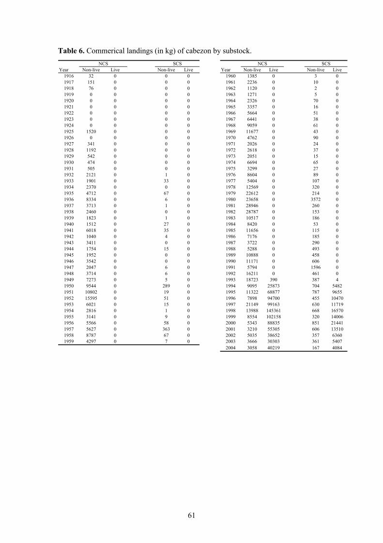
Table 6. Commerical landings (in kg) of cabezon by substock.

61

Year Non-live Live3 010 02 05 070 016 051 038 061 043 090 024 037 015 065 027 089 0

107 0320 0214 0

3572 0260 0153 0186 053 0

115 0185 0290 0493 0458 0606 0

1596 0461 0387 4704 5482787 9655455 10470630 11719668 16570320 14006851 21441606 13510357 6360361 5407167 4084

SCSNon-live Live Non-live Live Year Non-live Live

1916 32 0 0 0 1960 1385 01917 151 0 0 0 1961 2236 01918 76 0 0 0 1962 1120 01919 0 0 0 0 1963 1271 01920 0 0 0 0 1964 2326 01921 0 0 0 0 1965 3357 01922 0 0 0 0 1966 5664 01923 0 0 0 0 1967 6441 01924 0 0 0 0 1968 9059 01925 1520 0 0 0 1969 11677 01926 0 0 0 0 1970 4762 01927 341 0 0 0 1971 2026 01928 1192 0 0 0 1972 2618 01929 542 0 0 0 1973 2051 01930 474 0 0 0 1974 6694 01931 505 0 0 0 1975 3299 01932 2121 0 1 0 1976 8604 01933 1901 0 33 0 1977 5404 01934 2370 0 0 0 1978 12569 01935 4712 0 67 0 1979 22612 01936 8334 0 6 0 1980 23658 01937 3713 0 1 0 1981 28946 01938 2460 0 0 0 1982 28787 01939 1823 0 1 0 1983 10517 01940 1512 0 27 0 1984 8420 01941 6018 0 35 0 1985 11656 01942 1040 0 4 0 1986 7176 01943 3411 0 0 0 1987 3722 01944 1754 0 15 0 1988 5288 01945 1952 0 0 0 1989 10888 01946 3542 0 0 0 1990 11171 01947 2047 0 6 0 1991 5794 01948 3714 0 6 0 1992 16211 01949 7273 0 5 0 1993 18723 3901950 9544 0 289 0 1994 9095 258731951 10802 0 19 0 1995 11322 688771952 15595 0 51 0 1996 7898 947001953 6021 0 15 0 1997 21149 991631954 2816 0 1 0 1998 13988 1453611955 3141 0 9 0 1999 8554 1021581956 5566 0 58 0 2000 5343 888351957 5627 0 363 0 2001 3210 553051958 8787 0 67 0 2002 5035 386521959 4297 0 7 0 2003 3666 30303

2004 3058 40219

NCS SCS NCS

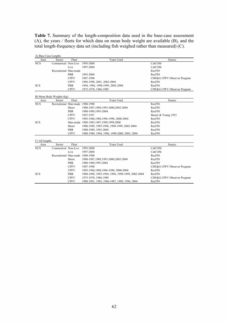
Table 7. Summary of the length-composition data used in the base-case assessment (A), the years / fleets for which data on mean body weight are available (B), and the total length-frequency data set (including fish weighed rather than measured) (C). A) Base Case Lengths

Area Sector Fleet Years Used SourceNCS Commerical Non-Live 1995-2000 CalCOM

Live 1997-2004 CalCOMRecreational Man-made RecFIN

PBR 1993-2004 RecFINCPFV 1987-1998 CDF&G CPFV Observer ProgramCPFV 1996-1998, 2001, 2003-2004 RecFIN

SCS PBR 1994, 1996, 1998-1999, 2002-2004 RecFINCPFV 1975-1978, 1986-1989 CDF&G CPFV Observer Program

B) Mean Body Weights (kg)Area Sector Fleet Years Used Source

NCS Recreational Man made 1980-1988 RecFINShore 1980-1987,1989,1993-2000,2002-2004 RecFINPBR 1980-1989,1993-2004 RecFINCPFV 1947-1951 Baxter & Young 1953CPFV 1985-1986,1988,1996-1998, 2000-2004 RecFIN

SCS Man-made 1980-1985,1987,1989,1999,2000 RecFINShore 1980-1989, 1995-1996, 1998-1999, 2002-2004 RecFINPBR 1980-1989, 1993-2004 RecFINCPFV 1980-1989, 1994, 1996, 1998-2000, 2003, 2004 RecFIN

C) All lengthsArea Sector Fleet Years Used Source

NCS Commerical Non-Live 1995-2000 CalCOMLive 1997-2004 CalCOM

Recreational Man made 1980-1988 RecFINShore 1980-1987,1989,1993-2000,2002-2004 RecFINPBR 1980-1989,1993-2004 RecFINCPFV 1987-1998 CDF&G CPFV Observer ProgramCPFV 1985-1986,1988,1996-1998, 2000-2004 RecFIN

SCS PBR 1980-1989, 1993-1994, 1996, 1998-1999, 2002-2004 RecFINCPFV 1975-1978, 1986-1989 CDF&G CPFV Observer ProgramCPFV 1980-1981, 1983, 1986-1987, 1989, 1996, 2004 RecFIN

62

63

Table 8. Catch length-compositions by substock, fishery sector, and fleet. N = original length-composition sample sizes before iterative re-weighting. Neff = base-case sample sizes after iterative re-weighting. Only measured lengths are included in this table. A) NCS

Sec 8 50 52 54 56 58 60 62 64 66 68 70 72+Commercial

01127 0.02995 0.02006 0.00962 0.00055 0.00605 0.00082 0 0 0.00082 0 0 003584 0.02059 0.01337 0.00856 0.00562 0.00508 0 0.00053 0 0 0 0 003156 0.03191 0.01786 0.01544 0.02549 0.02445 0.02445 0 0.01335 0 0 0 004456 0 0.00637 0 0 0 0 0 0.00000 0 0 0 0

0 0.03336 0 0.02294 0 0 0 0 0 0 0 0 009247 0.02146 0.05462 0.05462 0 0.02146 0 0 0 0.02731 0 0 004348 0.04348 0.02174 0.01449 0.00725 0.01449 0 0.00725 0 0 0 0 001994 0.01169 0.0054 0.00773 0.00661 0.00253 0.00108 0 0 0 0 0 003948 0.0262 0.01865 0.01649 0.00644 0.00752 0.00291 0.00096 0.00008 0 0 0 003747 0.02311 0.02402 0.00972 0.00544 0.00382 0.00171 0.00181 0.00031 0 0 0 004096 0.0208 0.0205 0.00702 0.00606 0.00394 0.00118 0 0.0003 0 0 0 006239 0.05915 0.04763 0.0268 0.02137 0.01515 0.0085 0 0.00269 0 0 0 000179 0.0764 0.06016 0.18049 0 0.06016 0.06016 0 0 0 0 0 000082 0.07678 0.00082 0.07615 0.00073 0.00036 0.00064 0 0 0 0 0 0

Recreational02941 0.02941 0 0.02941 0.05882 0 0 0 0 0 0 0 0

0 0 0 0 0.04762 0 0 0 0 0 0 0 00 0 0 0 0 0 0 0.05882 0 0 0 0 00 0.02703 0.02703 0 0 0 0 0 0 0 0 0 00 0 0 0 0 0 0 0 0 0 0 0 00 0.05263 0.02632 0 0 0 0 0 0 0 0 0 0

0 0 0 0 0 0 0 0 0 0 00 0 0 0 0 0 0 0 0 0 00 0 0 0 0 0 0 0 0 0 0

12500 0.12500 0 0 0 0 0 0 0 0 0 0 00.2 0 0 0 0 0 0 0 0 0 0 0 00 0.14286 0.07143 0 0.07143 0 0 0 0 0 0 0 0

01613 0.03226 0.03226 0.01613 0.03226 0 0 0.01613 0 0 0 0 00 0 0.01724 0.01724 0.03448 0.01724 0.01724 0.01724 0 0 0 0 0

02000 0.02000 0.04000 0.02000 0.04000 0.04000 0.02000 0 0 0 0 0 0.0678 0.0339 0.05085 0.0339 0.0339 0.0339 0 0 0 0.01695 0 0 0

0 0 0 0 0 0 0 0 0 0 0 0 009677 0 0 0 0.06452 0 0 0 0 0 0 0 006667 0 0.03333 0.03333 0 0 0 0 0 0 0 0 018182 0.09091 0 0.04545 0.04545 0 0 0.04545 0 0 0 0 008333 0.08333 0.04167 0.04167 0 0.04167 0 0 0 0 0 0 0

0 0.16667 0 0.05556 0 0.05556 0 0.05556 0 0.05556 0 0 014583 0.10417 0.0625 0.08333 0 0.04167 0 0.02083 0 0 0 0 01378 0.12598 0.06299 0.05118 0.05118 0.02362 0.01969 0 0.00787 0.00394 0.00394 0 0

CPFV (O 15625 0.09375 0.09375 0.0625 0.0625 0.15625 0 0.03125 0 0 0 0 005000 0.06250 0.12500 0.02500 0.02500 0.05000 0 0.01250 0.02500 0.01250 0 0 009459 0.10811 0.05405 0.05405 0.05405 0.01351 0.01351 0 0.01351 0 0 0 009091 0.09091 0 0 0.09091 0 0.09091 0 0 0 0 0 005556 0 0.05556 0.05556 0.16667 0.05556 0 0 0 0 0 0 006667 0.06667 0 0.03333 0 0 0.03333 0 0 0 0 0 009375 0.0625 0.0625 0 0.03125 0 0 0 0 0 0 0 002439 0 0.04878 0.04878 0 0 0.02439 0 0.02439 0 0 0 005405 0.08108 0 0.02703 0 0.02703 0 0 0 0 0 0 006542 0.05607 0.02804 0 0.00935 0 0.00935 0.00935 0 0 0 0 001695 0 0.03390 0 0.01695 0 0.01695 0 0 0 0 0 004878 0.02439 0 0 0 0 0 0 0 0 0 0 0

CPFV (RecF 12500 0 0 0.06250 0.12500 0 0.06250 0 0 0 0 0.06250 004000 0 0.08000 0 0 0 0 0 0 0 0 0 0

1998 17 17 0 0 0 0 0 0 0 0 0 0 0.03846 0 0.03846 0.03846 0.07692 0.19231 0.26923 0.15385 0.03846 0.11538 0 0 0 0.03846 0 0 0 0 0 0 0 0 0 02001 20 17 0 0 0 0 0 0 0 0 0 0 0 0 0 0 0.02632 0.02632 0.07895 0.10526 0.13158 0.02632 0.21053 0.18421 0.10526 0.02632 0.05263 0.02632 0 0 0 0 0 0 0 02003 26 37 0 0 0 0 0 0 0 0 0 0 0 0 0 0 0 0.01786 0.10714 0.07143 0.10714 0.14286 0.17857 0.05357 0.08929 0.08929 0.03571 0.03571 0.01786 0.01786 0.01786 0 0 0 0 0.017862004 16 36 0 0 0 0 0 0 0 0 0 0 0.04167 0.04167 0 0 0 0 0.04167 0.16667 0.125 0.08333 0.16667 0.16667 0.04167 0.08333 0 0 0 0 0 0 0.04167 0 0 0

tor Year N Neff 6 8 10 12 14 16 18 20 22 24 26 28 30 32 34 36 38 40 42 44 46 4

Non-live 1995 206 95 0 0 0 0 0 0 0 0 0 0 0.07007 0.05798 0.10387 0.11267 0.09068 0.12036 0.08079 0.08272 0.04534 0.13877 0.01759 0.1996 1696 1916 0 0 0 0 0 0 0 0.00053 0.00053 0.00749 0.023 0.06499 0.13613 0.15967 0.13533 0.11821 0.08264 0.05456 0.04547 0.04012 0.04172 0.1997 396 85 0 0 0 0 0 0 0 0 0 0.00069 0.00399 0.01474 0.07804 0.12244 0.10302 0.12244 0.0914 0.08498 0.10545 0.02601 0.06226 0.1998 46 39 0 0 0 0 0 0 0 0 0 0 0.00686 0.00686 0.06293 0.09941 0.18438 0.14716 0.13418 0.21425 0.0524 0.01616 0.02449 0.1999 51 4 0 0 0 0 0 0 0 0 0 0 0 0 0 0 0.05588 0.22602 0.19016 0.17181 0.17264 0.09591 0.031282000 112 4 0 0 0 0 0 0 0 0 0 0 0 0 0 0 0 0.13188 0.20211 0.09871 0.09871 0.12017 0.07647 0.

Live 1997 514 75 0 0 0 0 0 0 0 0 0 0 0 0 0 0.00725 0.1087 0.12319 0.18841 0.12319 0.15942 0.06522 0.07246 0.1998 1338 27 0 0 0 0 0 0 0 0 0 0 0.00386 0.0198 0.06022 0.08788 0.1658 0.18844 0.15045 0.10312 0.09671 0.03758 0.03118 0.1999 1450 123 0 0 0 0 0 0 0 0 0 0.00067 0 0.00091 0.00037 0.00395 0.0364 0.2263 0.21196 0.15428 0.11703 0.08334 0.04606 0.2000 2810 298 0 0 0 0 0 0 0 0 0 0 0.00024 0.00063 0.0013 0.00192 0.08805 0.20847 0.18594 0.15682 0.09852 0.08993 0.06075 0.2001 2101 83 0 0 0 0 0 0 0 0 0 0 0 0 0 0.0003 0.02161 0.09625 0.23274 0.20812 0.15121 0.1169 0.07212 0.2002 1288 41 0 0 0 0 0 0 0 0 0 0 0 0 0 0 0 0.08137 0.21831 0.1316 0.11103 0.10026 0.11376 0.2003 762 15 0 0 0 0 0 0 0 0 0 0 0 0 0 0 0 0.03104 0.15447 0.16724 0.0727 0.07891 0.05646 0.2004 1036 9 0 0 0 0 0 0 0 0 0 0 0 0 0 0 0 0.00682 0.02163 0.25906 0.31331 0.23871 0.00418 0.

Shore 1993 27 43 0 0 0 0 0.02941 0 0 0 0.02941 0 0 0.02941 0.02941 0.08824 0.14706 0.14706 0.14706 0.08824 0.02941 0.05882 0.02941 0.1994 15 11 0 0 0 0 0 0.09524 0.04762 0 0 0 0 0.04762 0.04762 0.04762 0.09524 0.2381 0.04762 0 0.19048 0.09524 01995 13 8 0 0 0 0 0 0 0.05882 0 0 0 0.05882 0 0 0.11765 0.17647 0.17647 0.05882 0.05882 0.17647 0.05882 01996 26 15 0 0 0 0 0 0 0 0 0 0.02703 0 0.02703 0.10811 0.10811 0.13514 0.18919 0.13514 0.10811 0 0.05405 0.054051997 20 32 0 0 0 0 0 0 0 0 0.06897 0 0.03448 0.03448 0.03448 0.13793 0.13793 0.13793 0.17241 0.03448 0.10345 0.10345 01998 20 12 0 0 0 0 0 0 0 0 0 0.02632 0.02632 0 0.02632 0.10526 0.13158 0.15789 0.21053 0.05263 0.13158 0.02632 0.026321999 16 13 0 0 0 0 0 0 0 0 0 0.03448 0 0.10345 0.10345 0.31034 0.17241 0.06897 0.06897 0.10345 0.03448 0 0 0 02000 5 12 0 0 0 0 0 0 0 0 0 0 0 0 0 0 0.625 0 0.25 0.125 0 0 0 0 02001 7 6 0 0 0 0 0 0 0 0 0 0.28571 0 0 0 0.14286 0 0 0 0.14286 0.42857 0 0 0 02002 5 8 0 0 0 0 0 0 0 0.12500 0 0.12500 0 0 0 0.12500 0 0 0 0.12500 0.12500 0 0.12500 0.2003 2 5 0 0 0 0 0 0 0 0 0 0 0 0 0.2 0.2 0 0 0 0.4 0 0 02004 10 11 0 0 0 0 0 0 0 0 0 0 0 0 0.14286 0 0.07143 0 0.07143 0.21429 0 0.14286 0.07143

PBR 1993 46 32 0 0 0 0 0 0 0 0.03226 0 0 0 0 0.01613 0.04839 0.08065 0.08065 0.24194 0.12903 0.16129 0.04839 0.01613 0.1994 44 47 0 0 0 0 0 0 0 0 0 0.01724 0.03448 0.05172 0 0.06897 0.05172 0.10345 0.15517 0.15517 0.10345 0.05172 0.086211995 32 24 0 0 0 0 0 0 0 0 0 0 0 0.02000 0.06000 0.10000 0.14000 0.10000 0.12000 0.08000 0.10000 0.04000 0.04000 0.1996 38 131 0 0 0 0 0 0 0 0 0.01695 0 0 0.01695 0.01695 0.08475 0.08475 0.0678 0.10169 0.0678 0.13559 0.0678 0.0678 01997 7 5 0 0 0 0 0 0 0 0 0 0 0 0 0 0 0 0 0.25000 0.25000 0.37500 0 0.125001998 24 32 0 0 0 0 0 0 0.03226 0 0 0.03226 0 0 0.06452 0.03226 0.06452 0.03226 0.19355 0.16129 0.16129 0.03226 0.03226 0.1999 28 32 0 0 0 0 0 0 0 0 0 0 0 0 0 0.13333 0.06667 0.03333 0.2 0.2 0.06667 0.13333 0.03333 0.2000 18 16 0 0 0 0 0 0 0 0 0 0 0 0 0 0 0.04545 0 0.09091 0.09091 0.04545 0.22727 0.09091 0.2001 17 16 0 0 0 0 0 0 0 0 0 0 0.04167 0 0 0 0.08333 0 0.04167 0.04167 0.08333 0.125 0.29167 0.2002 12 20 0 0 0 0 0 0 0 0 0 0 0 0 0.05556 0 0 0.05556 0.16667 0.05556 0.11111 0.05556 0.111112003 37 49 0.02083 0 0 0 0 0 0 0 0 0 0 0 0 0 0 0 0.125 0.125 0.10417 0.0625 0.10417 0.2004 153 113 0 0 0 0 0 0 0 0 0 0 0 0 0.00394 0.00394 0.01181 0.01969 0.04331 0.08268 0.09055 0.09843 0.15748 0.

bserver) 1987 32 17 0 0 0 0 0 0 0 0 0 0 0 0 0 0 0 0.03125 0 0.09375 0.0625 0.09375 0.0625 0.1988 80 45 0 0 0 0 0 0 0 0 0 0 0.01250 0.02500 0.02500 0 0.01250 0.03750 0.05000 0.07500 0.07500 0.10000 0.20000 0.1989 74 82 0 0 0 0 0 0 0 0 0 0 0 0.01351 0.01351 0.02703 0.04054 0.10811 0.02703 0.10811 0.10811 0.04054 0.10811 0.1990 11 17 0 0 0 0 0 0 0 0 0 0 0 0 0 0.09091 0 0 0 0.27273 0.09091 0.09091 0.09091 0.1991 18 19 0 0 0 0 0 0 0 0 0 0 0 0 0 0 0 0.05556 0.11111 0.16667 0.11111 0.05556 0.11111 0.1992 30 22 0 0 0 0 0 0 0 0 0 0 0 0 0 0.03333 0.1 0.2 0.03333 0.16667 0.13333 0.06667 0.06667 0.1993 32 67 0 0 0 0 0 0 0 0 0 0 0 0 0 0.0625 0.09375 0.0625 0.125 0.1875 0.09375 0.09375 0.03125 0.1994 41 28 0 0 0 0 0 0 0 0 0 0 0 0 0.04878 0 0.14634 0.17073 0.04878 0.09756 0.12195 0.09756 0.09756 0.1995 37 31 0 0 0 0 0 0 0 0 0 0 0 0.02703 0.02703 0.02703 0.02703 0.16216 0.08108 0.18919 0.08108 0.16216 0.02703 0.1996 107 102 0 0 0 0 0 0 0 0 0.00935 0 0 0.00935 0.05607 0.13084 0.09346 0.1028 0.1215 0.09346 0.07477 0.06542 0.06542 0.1997 59 21 0 0 0 0 0 0 0 0 0 0.01695 0 0 0 0.01695 0.08475 0.27119 0.10169 0.15254 0.10169 0.01695 0.15254 0.1998 41 35 0 0 0 0 0 0 0 0 0 0 0.02439 0 0.02439 0.02439 0.07317 0.17073 0.14634 0.19512 0.04878 0.12195 0.09756 0.

IN) 1996 13 20 0 0 0 0 0 0 0 0 0 0 0 0 0.06250 0 0.06250 0 0.06250 0.06250 0.12500 0.06250 0.12500 0.1997 15 18 0 0 0 0 0 0 0 0 0 0.04000 0 0 0 0 0.04000 0.16000 0.08000 0.20000 0.08000 0.04000 0.24000 0.

Length bin

Table 8 continued. B) SCS

Sector Year N Neff 6 8 10 12 14 16 18 20 22 24 26 28 30 32 34 36 38 40 42 44 46 48 50 52 54 56 58 60 62 64 66 68+Length bin

RecreationalPBR 1994 7 17 0 0 0 0 0 0 0 0 0 0 0 0 0.06667 0.13333 0.2 0.06667 0.06667 0.06667 0 0.06667 0 0.06667 0 0 0.06667 0.06667 0 0.13333 0 0 0 0

1996 10 42 0 0 0 0 0 0 0 0 0 0.03448 0.03448 0.13793 0.2069 0.2069 0.13793 0.03448 0.13793 0 0.03448 0 0 0 0 0 0 0 0 0 0.03448 0 0 01998 7 12 0 0 0 0 0 0 0 0 0 0 0.09524 0.04762 0 0.28571 0.28571 0.14286 0 0.09524 0.04762 0 0 0 0 0 0 0 0 0 0 0 0 01999 16 40 0 0 0 0 0 0 0.02500 0 0.02500 0.02500 0 0.07500 0.02500 0.12500 0.25000 0.17500 0.12500 0.05000 0.05000 0.02500 0 0 0 0.02500 0 0 0 0 0 0 0 02002 11 17 0 0 0 0 0 0 0 0 0 0 0 0 0.27273 0.22727 0.22727 0.04545 0.04545 0 0.04545 0.09091 0 0 0 0.04545 0 0 0 0 0 0 0 02003 12 45 0 0 0 0 0 0 0 0 0 0 0 0.03448 0.03448 0.17241 0.2069 0.17241 0.10345 0.13793 0 0.03448 0.03448 0 0.03448 0.03448 0 0 0 0 0 0 0 02004 41 42 0 0 0 0 0 0 0 0 0 0.00862 0 0.01724 0.06034 0.07759 0.11207 0.08621 0.10345 0.16379 0.08621 0.07759 0.06034 0.0431 0.03448 0.02586 0.02586 0 0.00862 0 0 0 0 0.00862

CPFV 1975 76 66 0 0 0 0 0 0 0.01316 0 0.01316 0.02632 0.09211 0.07895 0.14474 0.17105 0.07895 0.11842 0.03947 0.07895 0.03947 0.02632 0.02632 0.02632 0 0.01316 0 0 0.01316 0 0 0 0 01976 95 83 0 0 0 0.01053 0 0 0 0.01053 0.01053 0.05263 0.06316 0.10526 0.18947 0.09474 0.06316 0.08421 0.05263 0.08421 0.03158 0.04211 0.02105 0.02105 0.04211 0 0.01053 0.01053 0 0 0 0 0 01977 76 83 0 0 0 0 0.01316 0 0 0 0 0.06579 0.11842 0.13158 0.14474 0.06579 0.09211 0.09211 0.05263 0.03947 0.05263 0.01316 0.03947 0.03947 0 0.01316 0.01316 0 0 0 0.01316 0 0 01978 101 142 0 0 0 0.00990 0 0 0.0198 0.0099 0 0.0495 0.0495 0.06931 0.11881 0.07921 0.10891 0.07921 0.0495 0.08911 0.07921 0.02970 0.02970 0.03960 0 0.03960 0.03960 0 0.00990 0 0 0 0 01986 82 124 0 0 0 0 0 0 0.0122 0.0122 0.07317 0.18293 0.15854 0.19512 0.17073 0.04878 0.03659 0.03659 0.03659 0 0.02439 0.0122 0 0 0 0 0 0 0 0 0 0 0 01987 100 68 0 0 0 0 0 0 0 0 0.02000 0.01000 0.13000 0.12000 0.25000 0.13000 0.12000 0.09000 0.09000 0.03000 0.01000 0 0 0 0 0 0 0 0 0 0 0 0 01988 65 63 0 0 0 0 0 0 0 0 0.01538 0.06154 0.04615 0.07692 0.12308 0.15385 0.12308 0.09231 0.10769 0.15385 0.01538 0.01538 0 0 0.01538 0 0 0 0 0 0 0 0 01989 93 81 0 0 0 0 0 0.01075 0 0.02151 0.06452 0.16129 0.16129 0.08602 0.09677 0.08602 0.06452 0.08602 0.03226 0.01075 0.03226 0.01075 0.01075 0.04301 0.02151 0 0 0 0 0 0 0 0 0

64

Table 9. Annual mean body weights of cabezon by substock and fleet. A)NCS

Fleet Year Mean weight (kg) CV Fleet Year Mean weight (kg) CVMan made 1980 0.77 1.23 PBR 1980 1.56 0.45

0.70 1981 2.02 0.830.75 1982 1.57 0.400.72 1983 1.62 0.440.76 1984 1.40 0.400.86 1985 1.56 0.390.74 1986 1.37 0.430.76 1987 1.38 0.440.86 1988 1.44 0.460.64 1989 1.33 0.540.98 1993 1.29 0.391.00 1994 1.43 0.520.52 1995 1.28 0.531.11 1996 1.27 0.511.29 1997 0.80 0.460.91 1998 1.23 0.400.87 1999 1.48 0.380.88 2000 1.46 0.360.83 2001 1.57 0.330.82 2002 1.33 0.460.20 2003 1.61 0.290.20 2004 1.83 0.440.20 CPFV 1947 2.27 0.500.73 1948 2.27 0.500.47 1949 2.27 0.500.69 1950 2.27 0.500.49 1951 2.27 0.500.58 1960 2.42 0.500.56 1980 1.64 0.320.51 1981 1.67 0.290.79 1983 2.33 0.450.68 1985 1.54 0.411.04 1986 1.79 0.800.62 1988 1.64 0.630.90 1989 1.07 0.290.51 1994 1.22 0.340.39 1995 2.44 0.420.45 1996 1.28 0.480.42 1997 1.13 0.500.54 1998 1.32 0.300.70 1999 1.59 0.290.01 2000 1.59 0.440.44 2001 1.58 0.330.36 2002 1.63 0.440.36 2003 1.55 0.30

2004 1.56 0.40

1981 0.691982 0.711983 0.721984 1.041985 0.551986 0.861987 0.751988 1.131989 0.621993 0.441994 0.801995 0.201996 0.331997 0.681999 0.262001 0.502002 0.632003 0.982004 0.93

Shore 1958 0.411960 0.411961 0.411980 1.071981 0.781982 1.031983 0.931984 0.971985 0.701986 0.981987 0.601988 0.721989 0.891993 0.921994 0.881995 0.871996 0.911997 1.161998 1.151999 0.952000 0.952001 0.882002 1.162003 1.272004 1.60

65

Table 9 (continued). B)SCS

Fleet Year Mean weight (kg) CV Fleet Year Mean weight (kg) CVMan made 1980 0.49 0.52 PBR 1980 1.29 0.49

1981 0.42 0.65 1981 1.26 0.511982 0.49 0.29 1982 1.06 0.571983 0.58 0.66 1983 0.82 0.531984 0.45 0.56 1984 1.04 0.431985 0.26 0.50 1985 1.14 0.721987 0.81 0.54 1986 0.84 0.661989 0.84 0.82 1987 1.07 0.651999 0.31 0.70 1988 0.78 0.372000 0.05 0.39 1989 1.10 0.56

Shore 1980 1.13 0.54 1993 0.47 0.231981 0.78 0.51 1994 1.20 0.691982 0.81 0.52 1995 0.67 0.281983 0.74 0.56 1996 0.68 0.351984 0.89 0.22 1997 1.42 0.521985 0.80 0.49 1998 0.76 0.111986 0.89 0.76 1999 0.68 0.461987 1.06 0.55 2000 1.66 0.521988 1.13 0.53 2001 0.68 0.161989 1.36 0.53 2002 0.79 0.631995 0.36 0.55 2003 0.98 0.421996 0.56 0.25 2004 1.20 0.571998 0.78 0.52 CPFV 1980 0.97 0.591999 0.76 0.32 1981 1.02 0.502002 1.59 0.53 1982 0.75 0.802003 0.69 0.15 1983 0.79 0.632004 0.67 0.05 1984 1.04 0.46

1985 0.56 0.501986 0.59 0.341987 1.16 0.431988 0.51 0.561989 0.69 0.651994 0.94 0.221996 0.65 0.151998 1.01 0.671999 0.46 0.272000 0.71 0.212003 2.17 0.382004 1.62 0.45

66

Table 10. Summary statistics for the data sources that could form the basis for abundance indices.

Area Data Source Years # Observations # Positives % Positive NCS CPFV Logbook CPUE 1957-2003 23993 6440 26.84% CPFV Observer CPUE 1988-1997 4546 236 5.19% RecFIN PBR* 1980-1989;1993-2004 113980 2100 1.84% Monterey Adult Survey* 1993-1998 103 77 74.76% TENERA Adult Survey* 1977-2002 85 79 92.94% CalCOFI oblique (C1) tow* 1951-1975 3257 82 2.52% CalCOFI oblique (CB) tow* 1978-2004 1171 18 1.54% SCS CPFV Logbook CPUE 1947-2003 32388 10305 31.82% RecFIN PBR* 1980-1989;1993-2004 97183 777 0.80% CalCOFI oblique (C1) tow* 1951-1975 25252 112 0.44% CalCOFI oblique (CB) tow* 1977-2004 8115 30 0.37% CalCOFI manta tow 1978,1980,1981,1984-2002 2380 344 14.45% Power Plant 1972-2002 6834 962 14.08% *Not used in the base case assessment

67

Table 11. AIC values for the different models considered when developing potential indices of abundance for the NCS. Binomial Lognormal Gamma

Model AIC AIC AIC NCS CPFV 1957-1961

Yr 2510 3088 -2342 Yr+Loc 2306 2932 -2480 Yr+Mo 2513 2993 -2527

Yr+Mo+Loc 2303 2829 -2664 1962-2003

Yr 27512 27709 -46429 Yr+Loc 26913 27068 -47314 Yr+Mo 27027 27483 -46864

Yr+Mo+Loc 26392 26786 -47708 1960-2003

Yr 28583 28954 -48693 Yr+Loc 27973 28285 -49595 Yr+Mo 28098 28700 -49189

Yr+Mo+Loc 27449 27971 -50055 1957-2003

Yr 30022 30832 -51545 Yr+Loc 29373 30126 -52449 Yr+Mo 29556 30528 -52121

Yr+Mo+Loc 28859 29758 -53005 MONTEREY

Yr 118 172 -35 Yr + Loc 120 190 -22 Yr + Mo 122 174 -33 Yr+Dep 123 171 -42

Yr+Loc+Dep 134 185 -32 Yr+Mo+Dep 129 176 -34 Yr+Mo+Loc 124 188 -23

Yr+Mo+Loc+Dep 141 187 -29 TENERA

Yr 68 200 227 Yr + Mo 76 181 214

Yr- Year; Mo- Month; Loc- Location; Dep- Depth

68

69

Table 12. AIC values for the different models considered when developing potential indices of abundance for the SCS. Binomial Lognormal Gamma

Model AIC AIC AIC SCS CPFV 1947-1961

Yr 8248 10047 -14458 Yr+Loc 7869 9607 -14904 Yr+Mo 7777 9826 -14768

Yr+Mo+Loc 7315 9363 -15373 1962-2003

Yr 36978 37553 -94978 Yr+Loc 34992 34739 -98741 Yr+Mo 36089 37169 -95471

Yr+Mo+Loc 33944 34064 -99558

1960-2003 Yr 38174 38582 -97845

Yr+Loc 36111 35800 -101619Yr+Mo 37269 38183 -98336

Yr+Mo+Loc 35033 35101 -102442

1947-2003 Yr 45226 47653 -119326

Yr+Loc 43243 44680 -123315Yr+Mo 43994 47079 -120049

Yr+Mo+Loc 41766 43800 -124455 CalCOFI

Yr 1929.86 1078.24 Yr+Day/Night 1838.51 1069.41

Yr+Day/Night+Lat 1769.81 1057.76 Yr+Lat 1868.8 1071.46

Yr+Long 1931.07 1080.08 Yr+Mo 1905.78 1077.1

Impingement

Yr 5494.07 2904.42 Yr+Mo 5607.46 3016.11

Yr+Season 4993.35 2682.41 Yr+Season+Station 4881.64 2620.23

Yr+Station 5380.96 2841.29

Yr- Year; Mo- Month; Loc- Location; Lat- Latitude; Long- Longitude

Table 13. Fishery-dependent and -independent abundance indices considered in the 2005 cabezon stock assessment for the NCS. The CVs are derived from a bootstrap procedure.

Year Index CV Index CV Index CV Index CV Index CV Index CV1957 0.06 0.26 0.0332 0.091958 0.04 0.22 0.0209 0.051959 0.03 0.20 0.0156 0.051960 0.02 0.22 0.01 0.08 0.0095 0.081961 0.02 0.25 0.01 0.07 0.0088 0.071962 0.01 0.11 0.01 0.11 0.0093 0.111963 0.02 0.14 0.02 0.13 0.0150 0.131964 0.02 0.15 0.02 0.15 0.0167 0.151965 0.02 0.08 0.02 0.08 0.0196 0.081966 0.02 0.10 0.02 0.11 0.0169 0.111967 0.01 0.09 0.01 0.09 0.0104 0.101968 0.01 0.09 0.01 0.10 0.0069 0.101969 0.01 0.14 0.01 0.15 0.0058 0.161970 0.01 0.17 0.01 0.18 0.0086 0.191971 0.01 0.09 0.01 0.09 0.0069 0.091972 0.01 0.10 0.01 0.10 0.0115 0.111973 0.01 0.12 0.01 0.11 0.0105 0.121974 0.01 0.08 0.01 0.09 0.0098 0.101975 0.01 0.07 0.01 0.07 0.0058 0.071976 0.01 0.19 0.01 0.19 0.0073 0.211977 0.01 0.12 0.01 0.12 0.0065 0.12 1.47 0.491978 0.01 0.11 0.01 0.11 0.0129 0.10 2.28 0.681979 1.73 0.231980 0.01 0.09 0.01 0.09 0.0098 0.10 1.52 0.401981 0.01 0.08 0.01 0.09 0.0063 0.09 1.09 0.481982 0.01 0.11 0.01 0.10 0.0052 0.11 1.54 0.471983 0.01 0.23 0.01 0.20 0.0054 0.23 1.42 0.521984 0.00 0.12 0.00 0.12 0.0028 0.13 0.77 0.581985 0.00 0.15 0.00 0.15 0.0020 0.14 1.55 0.381986 0.00 0.27 0.00 0.26 0.0041 0.27 4.48 0.621987 0.01 0.11 0.01 0.11 0.0057 0.11 2.28 0.761988 0.01 0.09 0.01 0.10 0.0071 0.10 1.85 0.371989 0.01 0.17 0.01 0.18 0.0055 0.19 2.16 0.461990 0.00 0.11 0.00 0.11 0.0043 0.12 2.52 0.381991 0.00 0.16 0.00 0.17 0.0033 0.18 3.49 0.281992 0.00 0.20 0.00 0.21 0.0044 0.21 1.70 0.381993 0.00 0.16 0.00 0.17 0.0032 0.18 0.11 0.38 0.92 0.541994 0.00 0.18 0.00 0.18 0.0021 0.18 0.25 0.32 0.83 0.521995 0.00 0.17 0.00 0.17 0.0021 0.16 0.21 0.43 1.42 0.461996 0.00 0.13 0.00 0.14 0.0034 0.15 0.08 1.01 0.84 0.581997 0.00 0.10 0.00 0.10 0.0042 0.11 0.25 0.29 1.83 0.341998 0.00 0.13 0.00 0.14 0.0035 0.15 0.15 0.50 1.02 0.551999 0.00 0.15 0.00 0.14 0.0043 0.152000 0.00 0.15 0.00 0.14 0.0033 0.14 0.78 0.282001 0.01 0.18 0.01 0.19 0.0060 0.19 0.88 0.362002 0.00 0.27 0.00 0.28 0.0023 0.29 0.57 0.472003 0.01 0.07 0.01 0.08 0.0091 0.08

Fishery IndependentNorthern California CPFV Monterey TENERAFishery Dependent

70

Table 14. Fishery dependent and independent abundance indices considered in the 2005 cabezon stock assessment for the SCS. The CVs are derived from a bootstrap procedure.

Year Index CV Index CV Index CV Index CV Index CV Index CV1947 0.000436 1.62 0.000817 1.771948 0.000968 0.34 0.001498 0.381949 0.000930 0.27 0.001438 0.211950 0.001173 0.25 0.001696 0.281951 0.001194 0.25 0.001601 0.251952 0.001560 0.26 0.001936 0.251953 0.002569 0.18 0.003053 0.141954 0.006878 0.16 0.006356 0.111955 0.008510 0.14 0.006688 0.111956 0.010580 0.24 0.009009 0.251957 0.005703 0.14 0.004561 0.101958 0.003395 0.11 0.003050 0.071959 0.000751 0.24 0.000888 0.191960 0.000220 0.35 0.0004 0.26 0.000394 0.241961 0.000487 0.42 0.0008 0.76 0.000733 0.601962 0.001614 0.14 0.0016 0.14 0.001627 0.141963 0.002329 0.23 0.0024 0.25 0.002318 0.231964 0.002292 0.09 0.0023 0.09 0.002320 0.091965 0.001840 0.08 0.0019 0.07 0.001865 0.081966 0.002447 0.39 0.0025 0.40 0.002492 0.381967 0.001742 0.11 0.0018 0.11 0.001781 0.111968 0.001051 0.28 0.0011 0.28 0.001075 0.291969 0.001110 0.24 0.0011 0.26 0.001128 0.271970 0.001092 0.17 0.0011 0.17 0.001114 0.171971 0.001328 0.20 0.0013 0.19 0.001371 0.201972 0.002351 0.40 0.0024 0.45 0.002436 0.44 13.57 0.221973 0.001159 0.18 0.0012 0.18 0.001207 0.16 17.22 0.201974 0.001586 0.12 0.0016 0.12 0.001634 0.12 6.52 0.181975 0.002205 0.12 0.0022 0.12 0.002288 0.10 9.38 0.151976 0.001708 0.11 0.0017 0.11 0.001760 0.10 7.12 0.161977 0.001127 0.08 0.0011 0.08 0.001156 0.08 4.39 0.231978 0.001440 0.10 0.0015 0.11 0.001476 0.10 63.18 0.70 3.31 0.211979 1.48 0.221980 0.001220 0.14 0.0012 0.13 0.001257 0.13 100.16 0.48 1.70 0.201981 0.001214 0.10 0.0012 0.10 0.001256 0.10 43.57 0.30 2.76 0.241982 0.000844 0.11 0.0009 0.11 0.000865 0.11 2.30 0.261983 0.000783 0.12 0.0008 0.11 0.000813 0.12 2.36 0.241984 0.000228 0.19 0.0002 0.19 0.000235 0.17 39.44 0.28 2.46 0.221985 0.000461 0.72 0.0005 0.70 0.000473 0.90 74.52 0.31 2.36 0.211986 0.001314 0.10 0.0013 0.10 0.001355 0.10 29.46 0.34 1.58 0.241987 0.001658 0.09 0.0017 0.09 0.001708 0.09 32.96 0.46 2.65 0.201988 0.001426 0.11 0.0014 0.11 0.001463 0.11 31.43 0.30 1.04 0.341989 0.002456 0.10 0.0025 0.09 0.002551 0.09 87.16 0.21 2.59 0.241990 0.002987 0.09 0.003 0.09 0.003098 0.09 44.32 0.50 1.73 0.261991 0.002035 0.09 0.0021 0.09 0.002113 0.08 85.75 0.32 2.39 0.231992 0.001186 0.07 0.0012 0.07 0.001217 0.07 16.66 0.67 1.51 0.241993 0.000726 0.12 0.0007 0.13 0.000739 0.13 16.82 0.50 0.56 0.341994 0.000445 1.21 0.0005 1.23 0.000458 1.26 16.66 0.58 0.80 0.361995 0.000626 0.16 0.0006 0.16 0.000649 0.15 30.34 0.38 0.84 0.441996 0.001143 0.20 0.0012 0.18 0.001195 0.19 33.24 0.35 0.76 0.431997 0.000828 0.15 0.0008 0.15 0.000859 0.14 46.69 0.37 1.32 0.391998 0.000338 0.16 0.0003 0.15 0.000351 0.14 3.16 0.29 0.77 0.411999 0.000338 0.18 0.0003 0.19 0.000351 0.19 52.95 0.29 5.87 0.222000 0.000636 0.69 0.0006 0.68 0.000652 0.77 40.23 0.36 4.26 0.322001 0.000826 0.14 0.0008 0.13 0.000852 0.13 29.37 0.37 6.02 0.492002 0.000434 0.26 0.0004 0.28 0.000443 0.29 112.91 0.34 8.27 0.292003 0.000375 0.18 0.0004 0.17 0.000407 0.18

Fishery Dependent Fishery IndependentSouthern California CPFV CalCOFI Impingement

71

Table 15. Input variables and parameters of the population dynamics model. The base-case values are given for those parameters that are pre-specified. An X indicates the parameter is estimated. Prior distributions for the parameters are listed in the SS2 control files (Appendices B-2 and C-2).

ParameterAge at minimum length (Lmin) 0 0Age at maximum length (Lmax) 17 17Natural Mortality (M ) 0.25(F)/0.3(M) 0.25(F)/0.3(M)Minimum Length (Lmin) 10.79(F)/16.93(M) 10.79(F)/16.93(M)Maximum Length (Lmax) 59.71(F)/46.56(M) 59.71(F)/46.56(M)Growth rate (k) 0.18(F)/0.28(M) 0.18(F)/0.28(M)Length at age 0 CV 0.14 0.14Length at age 17 CV 0.09 0.09lnRO X Xsteepness (h ) 0.7 0.7

1 1Recruitment (years) (1980-2003) (1970-2003)Selectivities

Commercial non-liveparameter 1 X NSC valueparameter 2 X NSC value

Commericial liveparameter 1 X NSC valueparameter 2 0 NSC valueparameter 3 X NSC valueparameter 4 X NSC valueparameter 5 X NSC valueparameter 6 X NSC valueparameter 7 X NSC valueparameter 8 1 NSC value

Recreational Man-madeparameter 1 X NSC valueparameter 2 0 NSC valueparameter 3 X NSC valueparameter 4 0.5 Xparameter 5 -0.5 NSC valueparameter 6 X Xparameter 7 X Xparameter 8 4 NSC value

Recreational Shoreparameter 1 X NSC valueparameter 2 0 NSC valueparameter 3 X NSC valueparameter 4 X Xparameter 5 X NSC valueparameter 6 X Xparameter 7 X Xparameter 8 4 NSC value

Recreational PBRparameter 1 X Xparameter 2 X X

Recreational CPFVparameter 1 X Xparameter 2 X X

CPFV surveyCalCOFI survey

parameter 1 0parameter 2 0

Impingement survey

mirrors Recreational CPFV mirrors Recreational CPFV

NCS SCSCabezon substock

Estimated in Base Case

Pre-specified in Base Case

Pre-specified in Base Case

Estimated in Base Case

parameter 1 0parameter 2 1

Rσ

72

Table 16. Comparison of total cabezon reproductive output (measured in spawning biomass (mt)) and depletion rates in California among the two current assessment models and previous assessment.

Model SB1916 SB1930 SB2003 SB2005 SB2003/SB1930 SB2005/SB1916

2005 Assessmenttwo substock model 1361 1353 542 516 40.0% 37.9%

one stock model 1268 1260 353 634 28.0% 50.0%one stock/all lengths 1245 1207 428 318 35.5% 25.5%

2003 Assessment 902 313 34.7%

Total California Cabezon Spawning Biomass (mt)

73

74

Table 17. Values for the likelihood components and summary statistics related to the current status of the resource for the sensitivity tests that involve changing the data sources included in the assessment (- data source is ignored) NCS

ikelihood Components Base Case 1 2 3 4 5 6 7 8dance Index

CPFV (1960-2003) 24.49 24.21 25.4 25.27 27.11 23.8 21.00 - -CPFV (1957-2003) - - - - - - - 28.98 -

V (1957-1961;1962-2003) - - - - - - - - 2.76/21.93Monterey adult survey - - - - - - - - -TENERA adult survey - - - - - - - - -

RecFIN PBR - - - - - - - - - Body Weight 21.75 21.74 20.29 17.57 17.54 13.76 13.44 21.70 21.12h Comps.

Commerical (non-live) 51.63 - 49.09 52.55 54.21 50.12 50.19 51.82 50.20

TrialL 9 10 11 12 13

Abun- 22.80 23.17 20.65 23.29- - - - -

CPF - - - - -- 2.40 - 2.11 -- 19.69 19.57 - -- - - - -

Mean 21.44 18.74 19.27 21.63 19.89Lengt

51.28 53.5 53.68 52.71 51.78Commerical (live) 51.98 46.7 - 48.55 43.61 52.85 50.11 54.37 52.32 51.69 50.86 49.76 50.29 51.18Rec: Shore-based 88.38 80.74 77.64 80.08 - 85.73 77.66 77.34 77.56 91.84 77.55 78.88 78.69 90.15

Rec: PBR 112.52 109.05 110.68 110 105.04 - 115.56 112.56 111.08 111.46 113.26 112.45 111.81 110.90Rec: CPFV 146 141.98 143.3 142.25 138.03 147.05 - 143.47 143.96 144.06 144.65 143.94 142.48 146.36

Recruitment penalty 6.91 6.25 7.59 6.74 6.71 5.29 11.12 6.47 7.04 7.76 8.96 8.85 7.19 8.25Parameter priors 6.05 5.12 4.99 4.47 2.98 2.53 4.12 3.31 3.33 1.98 2.16 2.02 1.99 3.37TOTAL LIKELIHOOD 509.7 435.78 380.72 487.57 395.25 381.24 343.2 500.04 490.69 481.50 514.56 511.58 489.55 505.191916 reproductive output 1110 (87) 1196 (118) 1104 (95) 1096 (89) 1133 (96) 1268 (105) 900 (106) 1091 (82) 1108 (88) 1057 (98) 917 (68) 921 (68) 1092 (87) 1063 (82)2005 reproductive output 445 (103) 390 (67) 404 (73) 372 (56) 414 (71) 534 (54) 324 (54) 396 (44) 443.72 (103) 398 (65) 276 (23) 264 (32) 448 (51) 447 (88)%Depletion 40.1 (7)% 41.4 (8)% 36.4 (8)% 38.1 (7)% 36.56 (7)% 42.1 (8)% 47.42 (11)% 36.3 (7)% 40.1 (7)% 37.6 (10)% 30.1 (6)% 28.7 (6)% 41.0 (8)% 42.0 (6)%

SCS

Likelihood Components Base Case 1 2 3 4 5 6 7 8 9 10 11 12Abundance Index

CPFV (1960-2003) 49.24 40.65 49.39 46.41 30.94 53.29 - - - 46.71 43.97 41.55 45.23CPFV (1947-2003) - - - - - - 82.45 - - - - -

CPFV (1947-1961;1962-2003) - - - - - - - 13.07/41.92 - - - -CalCOFI larval tows 10.03 9.20 10.17 9.93 9.90 6.01 8.57 14.08 9.03 - 12.16 - 15.30

Impingement 14.01 15.28 14.19 13.95 14.11 11.79 12.56 13.02 9.26 16.64 - - 20.59RecFIN PBR

Mean Body Weight 62.27 36.12 62.25 53.13 38.38 51.58 67.69 57.30 42.97 57.07 59.90 55.50 76.69Length Comps.

Rec: PBR 70.64 63.68 70.71 66.77 - 73.66 72.89 69.48 68.16 68.82 70.12 69.30 73.05Rec: CPFV 86.99 85.28 86.87 85.96 87.20 - 87.29 91.09 95.78 84.95 87.18 85.21 87.79

Recruitment penalty 26.69 20.79 26.34 22.04 21.29 16.04 24.23 22.25 20.53 27.99 25.00 28.02 34.77Parameter priors 4.45 4.25 4.23 4.29 4.20 5.85 4.31 4.73 4.32 4.64 5.22 5.13 4.53TOTAL LIKELIHOOD 324.41 275.26 324.15 302.48 206.34 218.22 359.99 326.88 250.05 306.82 303.58 284.71 357.431916 reproductive output 251 (21) 230 (21) 250 (21) 248 (23) 264 (22) 318 (30) 261 (19) 314 (25) 381 (30) 230 (23) 237 (22) 210 (18) 216 (14)2005 reproductive output 71 (15) 13 (7) 74 (16) 84 (18) 69 (15) 76 (17) 62 (13) 90 (19) 154 (42) 66 (15) 60 (14) 56 (14) 63 (12)%Depletion 28.3 (6)% 5.8 (3)% 29.7 (6)% 34.1 (7)% 26.2 (6)% 23.9 (5)% 23.4 (5)% 28.5 (6)% 40.5 (11)% 28.7 (7)% 25.3 (6)% 26.5 (6)% 29.0 (5)%

Trial

75

RTable 18. Results of the sensitivity tests in which the (pre-specified) values for M and σ are varied. The results in bold typeface pertain to the base case analyses. NCS

Fe

SCS

Fe

Negative Logmale Male σ R SB1916 SB2005 Depletion Likelihood0.2 0.25 0.5 1006 359 35.69% 519.04

1 1065 326 30.61% 508.941.5 1059 295 27.86% 510.93

0.25 0.25 0.5 892 499 55.94% 523.551 1065 473 44.41% 510.41

1.5 1151 402 34.93% 509.070.25 0.3 0.5 954 373 39.10% 520.12

1 1110 445 40.10% 509.701.5 1164 383 32.90% 508.15

0.3 0.35 0.5 1003 686 68.39% 526.691 1265 619 48.93% 507.67

1.5 1479 520 35.16% 505.170.2 0.35 0.5 1118 344 30.77% 518.51

1 1135 304 26.78% 509.031.5 1141 282 24.72% 513.53

Negative Logmale Male σ R SB1916 SB2005 Depletion Likelihood0.2 0.25 0.5 327 59 18.00% 371.13

1 261 67 25.50% 355.131.5 242 71 29.29% 363.16

0.25 0.25 0.5 237 55 23.31% 335.961 220 63 28.65% 329.70

1.5 209 65 30.94% 340.860.25 0.3 0.5 263 56 21.47% 326.14

1 251 71 28.27% 324.421.5 239 68 28.56% 334.38

0.3 0.35 0.5 213 59 27.69% 307.261 238 68 28.72% 302.32

1.5 235 66 27.99% 315.820.2 0.35 0.5 379 62 16.40% 358.63

1 306 69 22.67% 348.421.5 290 76 26.20% 352.15

M

M

Table 19. Results of the sensitivity tests in which changes are made to: a) the years for which recruitment residuals are estimated, b) the specifications for length/age-specific selectivity, c) the length data included in the analyses, d) the historical catches, e) the coefficients of variation assumed for the abundance indices and the effective sample sizes assumed for the length-composition data, and f) the coefficients of variation assumed for length-at-age.

Negative Log NegatSB1916 SB2005 Depletion Likelihood SB1916 SB2005 Depletion Lik

Base Case 1110 445 40.09% 510.00 Base Case 251 71 28.27% 3Recruitment Year Recruitment Year

start:1916 1693 512 30.27% 500.29 start:1916 432 76 17.55% 28start:1947 1608 512 31.82% 499.97 start:1960 401 79 19.68% 30start:1970 1354 519 38.31% 502.26 start:1980 259 69 26.74% 32start:1990 753 223 29.53% 527.14 end: 2002 243 69 28.59% 37end: 2002 1130 468 41.43% 507.56 end: 2004 246 73 29.65% 32end: 2004 1107 428 38.67% 506.01

Logositic SelectivityLogisitic Selectivity all fleets 231 50 21.61% 3

all fleets 1014 454 44.74% 532.36 fleet 3 & 4 236 73 31.04% 35fleet 3 & 4 1014 453 44.73% 531.88

CalCOFI selectivityAll lengths 962 324 33.64% 708.75 selectivity= female maturity 231 68 29.32% 3

Original CV/Neff 1014 453 44.73% 531.88 All lengths 283 59 20.97% 32Max Neff = 200 1292 534 41.33% 627.82

Original CV/Neff 236 73 31.04% 3Catch history Max Neff = 200 257 72 28.02% 3

Halved 747 351 47.05% 512.29Double 1858 720 38.73% 503.84 Catch history

Numbers 1709 744 43.53% 507.01 Halved 136 29 21.50% 3Double 431 105 24.48% 33

Length at age CV (both sexes) Numbers 266 84 31.56% 310.05 1456 618 42.47% 537.95 1980 catch 226 66 29.12% 31

0.2 664 157 23.70% 534.090.2/0.05 1213 542 44.67% 524.47 Length at age CV (both sexes)0.05/0.2 781 197 25.16% 521.70 0.05 317 86 27.19% 36

0.09/0.014 960 306 31.94% 507.29 0.2 189 26 13.98% 30.2/0.05 248 70 28.08% 30.05/0.2 254 58 23.03% 31

0.09/0.014 257 62 24.09% 31

NCS SCSive Log

elihood24.42

9.221.466.120.321.85

51.898.53

12.63

2.73

58.5349.78

25.984.817.079.05

4.8126.3530.739.376.57

76

Table 20. Projections (2006–16) of harvest levels, age 2+ biomass, spawning biomass and depletion for each substock under two different control rules/FMSY proxies. A) NCS

Year OY ABC SB2+ SB Depletion OY ABC SB2+ SB Depletion2005 59 107 727 440 40% 59 90 727 440 40%

tion

40-10/F45% 60-20/F50%

2006 59 90 684 393 35% 59 78 684 393 35%2007 84 81 655 360 32% 44 71 655 360 32%2008 76 78 655 327 29% 43 70 691 351 32%2009 77 81 684 321 29% 48 73 746 363 33%2010 84 86 721 335 30% 58 78 805 390 35%2011 91 92 755 354 32% 68 83 857 420 38%2012 97 96 782 370 33% 77 88 900 445 40%2013 102 100 803 383 34% 84 91 934 465 42%2014 105 103 821 392 35% 89 95 960 481 43%2015 108 105 834 400 36% 93 97 981 494 44%2016 110 107 845 406 37% 96 100 997 503 45%

B) SCS

Year OY ABC SB2+ SB Depletion OY ABC SB SB2+ Deple2005 10 24 197 72 29% 10 21 197 72 29%2006 10 27 217 90 36% 10 23 217 90 36%2007 30 26 226 112 45% 22 23 226 112 45%2008 29 25 219 111 45% 22 23 227 116 46%2009 28 25 214 106 43% 21 23 228 115 46%2010 27 25 211 103 41% 21 23 230 115 46%2011 27 25 209 101 40% 22 23 232 116 46%2012 27 25 207 100 40% 22 23 234 117 47%2013 27 25 206 100 40% 22 24 235 118 47%2014 26 26 205 99 40% 23 24 237 118 47%2015 26 26 204 99 39% 23 24 237 119 48%2016 26 26 204 98 39% 23 24 238 120 48%

40-10/F45% 60-20/F50%

77

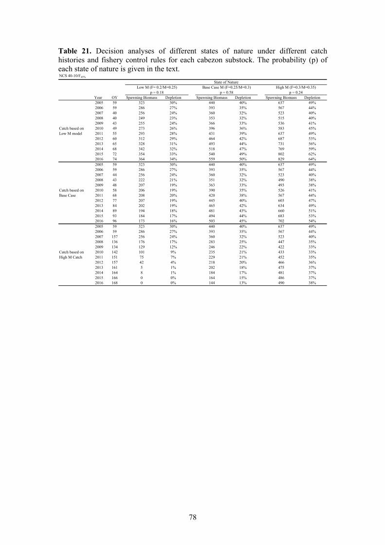
Table 21. Decision analyses of different states of nature under different catch histories and fishery control rules for each cabezon substock. The probability (p) of each state of nature is given in the text. NCS 40-10/F45%

Year OY Spawning Biomass Depletion Spawning Biomass Depletion Spawning Biomass Depletion2005 59 323 30% 440 40% 637 49%2006 59 286 27% 393 35% 567 44%2007 40 256 24% 360 32% 523 40%2008 40 249 23% 353 32% 515 40%2009 43 255 24% 366 33% 536 41%


2012 60 312 29% 464 42% 687 53%2013 65 328 31% 493 44% 731 56%2014 68 342 32% 518 47% 769 59%2015 72 354 33% 540 49% 802 62%2016 74 364 34% 559 50% 829 64%2005 59 323 30% 440 40% 637 49%2006 59 286 27% 393 35% 567 44%2007 44 256 24% 360 32% 523 40%2008 43 222 21% 351 32% 490 38%2009 48 207 19% 363 33% 493 38%


2012 77 207 19% 445 40% 603 47%2013 84 202 19% 465 42% 634 49%2014 89 194 18% 481 43% 660 51%2015 93 184 17% 494 44% 683 53%2016 96 173 16% 503 45% 702 54%2005 59 323 30% 440 40% 637 49%2006 59 286 27% 393 35% 567 44%2007 157 256 24% 360 32% 523 40%2008 136 176 17% 283 25% 447 35%2009 134 129 12% 246 22% 422 33%


2012 157 42 4% 218 20% 466 36%2013 161 5 1% 202 18% 475 37%2014 164 8 1% 184 17% 481 37%2015 166 0 0% 164 15% 486 37%2016 168 0 0% 144 13% 490 38%

State of NatureLow M (F= 0.2/M=0.25)

p = 0.18High M (F=0.3/M=0.35)

p = 0.24Base Case M (F=0.25/M=0.3)

p = 0.58

78

Table 21 continued. NCS 60-20/F50%

OYState of Nature

Low M (F= 0.2/M=0.25) Base Case M (F=0.25/M=0.3) High M (F=0.3/M=0.35)Commerical



2012 57 306 29% 459 41% 684 53%2013 60 325 30% 490 44% 730 56%2014 63 341 32% 519 47% 770 59%2015 65 356 33% 544 49% 806 62%2016 67 370 35% 566 51% 836 65%2005 59 323 30% 440 40% 637 49%2006 59 286 27% 393 35% 567 44%2007 44 256 24% 360 32% 523 40%2008 43 247 23% 351 32% 513 40%2009 48 251 24% 363 33% 533 41%


2012 77 292 27% 445 40% 670 52%2013 84 298 28% 465 42% 706 55%2014 89 301 28% 481 43% 736 57%2015 93 301 28% 494 44% 760 59%2016 96 299 28% 503 45% 780 60%2005 59 323 30% 440 40% 637 49%2006 59 286 27% 393 35% 567 44%2007 101 256 24% 360 32% 523 40%2008 89 212 20% 317 29% 480 37%2009 92 190 18% 304 27% 478 37%


2012 129 155 15% 322 29% 560 43%2013 136 132 12% 319 29% 577 45%2014 141 105 10% 313 28% 590 46%2015 144 75 7% 304 27% 599 46%2016 147 44 4% 294 26% 606 47%

p = 0.18 p = 0.58 p = 0.24

SCS 40-10/F45%

State of NatureOY

CommericalYear Removals Spawning Biomass Depletion Spawning Biomass Depletion Spawning Biomass Depletion2005 10 51 21% 72 29% 89 35%2006 10 63 26% 90 36% 110 43%2007 20 78 31% 112 45% 132 52%2008 20 80 32% 117 47% 137 54%2009 20 79 32% 117 47% 136 54%


2012 23 86 35% 119 48% 135 54%2013 23 88 36% 120 48% 134 53%2014 24 89 36% 120 48% 134 53%2015 24 90 37% 120 48% 132 52%2016 24 92 37% 120 48% 131 52%2005 10 51 21% 72 29% 89 35%2006 10 63 26% 90 36% 110 43%2007 30 78 31% 112 45% 132 52%2008 29 74 30% 111 45% 131 52%2009 28 69 28% 106 43% 125 50%


2012 27 66 27% 100 40% 116 46%2013 27 66 27% 100 40% 114 45%2014 26 67 27% 99 40% 113 45%2015 26 67 27% 99 39% 112 44%2016 26 67 27% 98 39% 111 44%2005 10 51 21% 72 29% 89 35%2006 10 63 26% 90 36% 110 43%2007 34 78 31% 112 45% 132 52%2008 32 73 29% 110 44% 129 51%2009 31 67 27% 104 42% 121 48%


2012 28 64 26% 98 39% 109 43%2013 28 64 26% 97 39% 107 42%2014 28 64 26% 97 39% 105 42%2015 27 65 26% 97 39% 104 41%2016 27 65 26% 96 39% 103 41%

Low (Depletion2005=0.2) Base Case High (Depletion2005=0.35)p = 0.16 p = 0.58 p = 0.26

79

Table 21 continued. SCS 60-20/F50%

OYCommerical



2012 18 103 42% 136 55% 152 60%2013 19 106 43% 138 55% 153 60%2014 20 109 44% 139 56% 152 60%2015 21 112 45% 140 56% 152 60%2016 21 113 46% 140 56% 151 60%2005 10 51 21% 72 29% 89 35%2006 10 63 26% 90 36% 110 43%2007 22 78 31% 112 45% 132 52%2008 22 79 32% 116 46% 136 54%2009 21 77 31% 115 46% 134 53%


2012 22 83 34% 117 47% 132 52%2013 22 85 35% 118 47% 132 52%2014 23 87 35% 118 47% 132 52%2015 23 89 36% 119 48% 132 52%2016 23 91 37% 120 48% 131 52%2005 10 51 21% 72 29% 89 35%2006 10 63 26% 90 36% 110 43%2007 27 78 31% 112 45% 132 52%2008 26 76 31% 116 46% 133 53%2009 25 72 29% 115 46% 128 51%


2012 24 74 30% 117 47% 123 49%2013 24 75 31% 118 47% 123 49%2014 23 77 31% 118 47% 123 49%2015 23 79 32% 119 48% 123 49%2016 23 80 33% 120 48% 122 49%

State of Nature

p = 0.16 p = 0.58 p = 0.26Low (Depletion2005=0.2) Base Case (F=0.25/M=0.3) High (Depletion2005=0.2)

80

120o

42o

40o

38o

A

36o

34o

32o

Figure 1. Map of the assesConception) and California Fislandmarks, cities, and islanhttp://www.dfg.ca.gov/mrd/fishisurveys used as indices of abund

CALIFORNI

sment areas (divided between NCS and SCS at Pt. h and Game regions (solid lines). Major fishing ports, ds are also distinguished. Map obtained from

ng_map.html. Red stars indicate where the adult fish ance were conducted.

81

http://www.dfg.ca.gov/mrd/fishing_map.html

0 2 4 6 8 10 12 14

prop

ortio

n m

atur

e

0.0

0.2

0.4

0.6

0.8

1.0

1.2

250 300 350 400 450 500 550 600

prop

ortio

n m

atur

e

0.0

0.2

0.4

0.6

0.8

1.0

1.2

ageAge (year)

leLength (mm) ngth mm Figure 2. Maturity of female cabezon versus age and length.

82

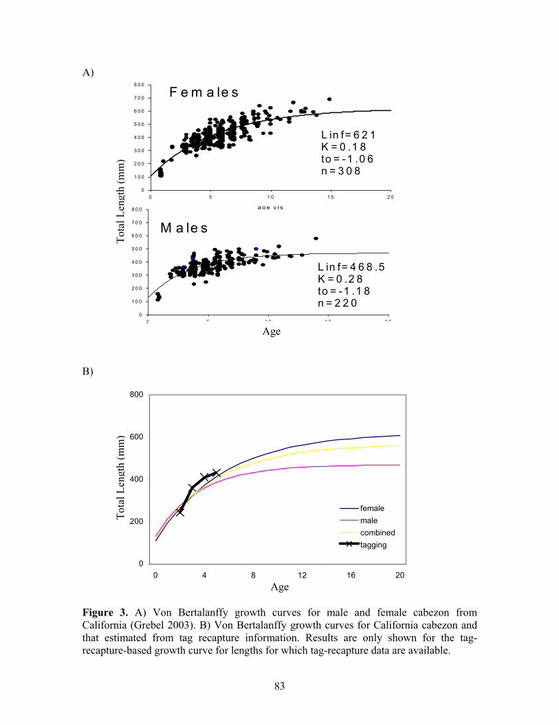
A) B)

Figure 3Californiathat estimrecapture-

0

200

400

600

800

0 4 8

F e m a le s

a g e y rs

0 5 1 0 1 5 2 00

1 0 0

2 0 0

3 0 0

4 0 0

5 0 0

6 0 0

7 0 0

8 0 0

M a le s

0 5 1 00

1 0 0

2 0 0

3 0 0

4 0 0

5 0 0

6 0 0

7 0 0

8 0 0

L in f= 6 2 1K = 0 .1 8to = -1 .0 6n = 3 0 8

Tota

l Len

gth

(mm

)

Ag

Tota

l Len

gth

(mm

)

A

. A) Von Bertalanffy growth (Grebel 2003). B) Von Bertalanated from tag recapture informbased growth curve for lengths fo

12 16 20

femalemalecombinedtagging

1 5 2 0

L in f= 4 6 8 .5K = 0 .2 8to = -1 .1 8n = 2 2 0

e

ge

curves for male and female cabezon from ffy growth curves for California cabezon and ation. Results are only shown for the tag-r which tag-recapture data are available.

83

LicensesPermits

1936 1938 1941 1943 1945 1947 1949

Year

Num

ber o

f CP

FV v

esse

ls

020

040

060

080

010

00

Figure 4. Registered Commercial Passenger Fishing Vessels (CPFVs) in California 1936–49 (source: Fishery Bulletins 57, 59, 63, 67, 74, 80).

84

1916 1925 1934 1943 1952 1961 1970 1979 1988 1997

Year

CP

FV R

emov

als

(in n

umbe

rs)

050

0010

000

1957-1978;1980-200319791936-1940;1947-19561941-19461929-1935

1916 1925 1934 1943 1952 1961 1970 1979 1988 1997

Year

CP

FV R

emov

als

(in n

umbe

rs)

020

0060

00

1957-1978;1980-200319791936-1940;1947-19561941-19461928-1935

A) NCS

B) SCS

Figure 5. Raw recreational removals by the CPFV mode: 1916–2004. Each color represents a different data source used when quantifying removals (see text for details).

85

1916 1925 1934 1943 1952 1961 1970 1979 1988 1997

Year

CP

FV R

emov

als

(in n

umbe

rs)

050

0015

000

1980-2003;1957-197819791947-1956;1936-19401941-19461929-1935

1916 1925 1934 1943 1952 1961 1970 1979 1988 1997

Year

CP

FV R

emov

als

(in n

umbe

rs)

020

0060

00 1980-2003;1957-197819791947-1956;1936-19401941-19461928-1935

A) NCS

B) SCS

Figure 6. Expanded recreational removals by the CPFV mode: 1916–2004. Each color represents a different data source used when quantifying removals (see text for details).

86

1916 1925 1934 1943 1952 1961 1970 1979 1988 1997

NCS

Year

Rec

reat

iona

l Rem

oval

s (in

kg)

010

0000

2000


1916 1925 1934 1943 1952 1961 1970 1979 1988 1997

SCS

Rec

reat

iona

l Rem

oval

s (in

kg)

Year

010

0000

2000


Figure 7. Removals (in kg) of cabezon by the recreational fishery by substock. .

87

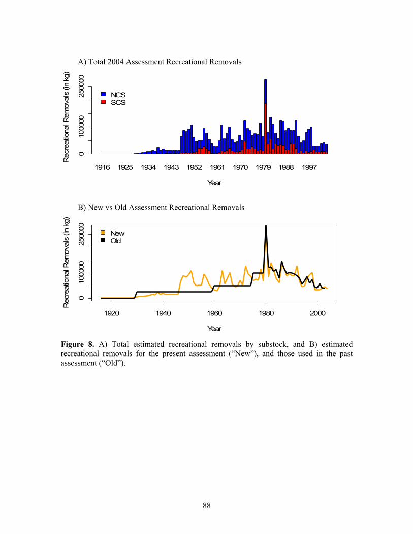
1916 1925 1934 1943 1952 1961 1970 1979 1988 1997

Year

Rec

reat

iona

l Rem

oval

s (in

kg)

010

0000

2500

00

NCSSCS

1920 1940 1960 1980 2000

010

0000

2500

00

Year

Rec

reat

iona

l Rem

oval

s (in

kg)

NewOld

A) Total 2004 Assessment Recreational Removals

B) New vs Old Assessment Recreational Removals

Figure 8. A) Total estimated recreational removals by substock, and B) estimated recreational removals for the present assessment (“New”), and those used in the past assessment (“Old”).

88

1 2 3 4 5 6

early Removals in kg by Wave

Rec

reat

iona

l Rem

oval

s (in

kg)

020

000

4000

0

1 2 3 4 5 6

RecFIN Wave

Ave

rage

wei

ght (

in k

g)

0.0

0.5

1.0

1.5

2.0

1 9 8 01 9 8 11 9 8 21 9 8 31 9 8 41 9 8 51 9 8 61 9 8 71 9 8 81 9 8 9

YA) Yearly Removals (in kg) by Wave

B) Yearly Average Weight (in kg) by Wave

Figure 9. Annual recreational removals (kg) by wave (upper panel), and annual average weights (kg) of removed fish by wave (1980–89) (lower panel).

89

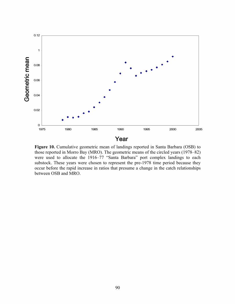
0

0.02

0.04

0.06

0.08

1

0.12

1975 1980 1985 1990 1995 2000 2005

Year

0.0.0.

Geo

met

ric m

ean

0

0.02

0.04

0.06

0.08

1

0.12

1975 1980 1985 1990 1995 2000 2005

Year

Geo

met

ric m

ean

0

0.02

0.04

0.06

0.08

1

0.12

1975 1980 1985 1990 1995 2000 2005

Year

Geo

met

ric m

ean

Figure 10. Cumulative geometric mean of landings reported in Santa Barbara (OSB) to those reported in Morro Bay (MRO). The geometric means of the circled years (1978–82) were used to allocate the 1916–77 “Santa Barbara” port complex landings to each substock. These years were chosen to represent the pre-1978 time period because they occur before the rapid increase in ratios that presume a change in the catch relationships between OSB and MRO.

90

1916 1925 1934 1943 1952 1961 1970 1979 1988 1997

Year

Com

mer

icia

l Rem

oval

s (in

kg)

050

000

1500

00Non-liveLive

mov

als

(in k

g)

1500

0 Non-liveLive

A) NCS

A) SCS

1916 1925 1934 1943 1952 1961 1970 1979 1988 1997

Year

Com

mer

icia

l Re

050

00

Figure 11. Commercial landings of cabezon by fleet and substock.

91

1916 1925 1934 1943 1952 1961 1970 1979 1988 1997

Year

Com

mer

icia

l Rem

oval

s (in

kg)

050

000

1500

00

NCS Non-liveNCS LiveSCS Non-liveSCS Live

1920 1940 1960 1980 2000

050

000

1500

00

Year

Com

mer

icia

l Rem

oval

s (in

kg)

NewOld

A) Total California Commercial Removals

B) New vs. Old Assessment Commercial Removals

Figure 12. A) Commercial landings by fleet and substock, and B) commercial landings used in the present (“New”) and past (“Old”) assessments.

92

1978 1983 1988 1993 1998 2003

Year

Non

-live

Com

mer

icia

l Rem

oval

s (in

kg)

040

000

8000

012

0000

1978 1983 1988 1993 1998 2003

Year

Live

Com

mer

icia

l Rem

oval

s (in

kg)

040

000

8000

012

0000

1978 1983 1988 1993 1998 2003

Year

Non

-Liv

e C

omm

eric

ial R

emov

als

(in k

g)

050

0015

000

2500

0

1978 1983 1988 1993 1998 2003

Year

Live

Com

mer

icia

l Rem

oval

s (in

kg)

010

000

2000

030

000

4000

0

FishHookSetTrawotherunk

pot and line

netl

nown

A) NCS

B) SCS

Figure 13. Commercial cabezon landings by fleet, substock and gear type.

93

1916 1924 1932 1940 1948 1956 1964 1972 1980 1988 1996

Year

Cat

ch (i

n kg

)

050

000

1000

0015

0000

JFMAMJJASOND

Figure 14. Commercial cabezon landings by three-month period: JFM: January, February, March; AMJ: April, May, June; JAS: July, August, September; OND: October, November, December.

94

1916 1928 1940 1952 1964 1976 1988 2000

Eureka

Year

Cat

ch (i

n kg

)

010

000

2500

0 JFMAMJJASOND

1916 1928 1940 1952 1964 1976 1988 2000

San Francisco

Year

Cat

ch (i

n kg

)

050

0015

000 JFM

AMJJASOND

1916 1928 1940 1952 1964 1976 1988 2000

Monterey

Year

Cat

ch (i

n kg

)

050

0015

000 JFM

AMJJASOND

1916 1928 1940 1952 1964 1976 1988 2000

Santa Barbara

Year

Cat

ch (i

n kg

)

040

000

8000

0

JFMAMJJASOND

1916 1928 1940 1952 1964 1976 1988 2000

Los Angeles

Year

Cat

ch (i

n kg

)

010

0020

0030

00

JFMAMJJASOND

1916 1928 1940 1952 1964 1976 1988 2000

San Diego

Year

Cat

ch (i

n kg

)

020

060

010

00

JFMAMJJASOND

Figure 15. Commercial cabezon landings by three-month period and port complex. The Santa Barbara complex includes Morro Bay (NCS) and Santa Barbara (SCS).

95

1916 1925 1934 1943 1952 1961 1970 1979 1988 1997

Year

Rem

oval

s (in

kg)

010

0000

2500

00 Rec. NCSRec. SCSComm. NCSComm. SCS

1920 1940 1960 1980 2000

010

0000

2500

00

Year

Rem

oval

s (in

kg)

NewOld

A) Total California Removals

B) New vs. Old Assessment Removals

Figure 16. Total cabezon removals A) by fishery sector and substock, and B) used in the present (“New”) and past (“Old”) assessment.

96

A) Non-Live

6 20 36 52 68

1995

Length (cm)

Proportion

0.00

0.02

0.04

0.06

0.08

0.10

0.12

6 20 36 52 68

1996

Length (cm)Proportion

0.00

0.05

0.10

0.15

6 20 36 52 68

1997

Length (cm)

Proportion

0.00

0.02

0.04

0.06

0.08

0.10

0.12

6 20

Lengt

Proportion

36 52 68

1998

h (cm)

0.00

0.05

0.10

0.15

0.20

6 20 36 52 68

1999

Length (cm)

Proportion

0.00

0.05

0.10

0.15

0.20

6 20 36 52 68

2000

Length (cm)

Proportion

0.00

0.05

0.10

0.15

0.20

1997

Proportion

0.00

0.05

0.10

0.15

1998

Proportion

0.00

0.05

0.10

0.15

1999

Proportion

0.00

0.05

0.10

0.15

0.20

Proportion

0.00

0.05

0.10

0.15

0.20

B) Live

6 20 36 52 68

2000

Length (cm)

6 20 36 52 68

Length (cm)

6 20 36 52 68

Length (cm)

6 20 36 52 68

Length (cm)

6 20 36 52 68

2001

Length (cm)

Proportion

0.00

0.05

0.10

0.15

0.20

6 20 36 52 68

2002

Length (cm)

Proportion

0.00

0.05

0.10

0.15

0.20

6 20 36 52 68

2003

Length (cm)

Proportion

0.00

0.05

0.10

0.15

6 20 36 52 68

2004

Length (cm)

Proportion

0.00

0.05

0.10

0.15

0.20

0.25

0.30

Figure 17. Commercial length compositions by fleet for the NCS.

97

A) Shore

6 20 36 52 68

1993

Length (cm)

Proportion

0.00

0.04

0.08

0.12

6 20 36 52 68

1994

Length (cm)

Proportion

0.00

0.10

0.20

6 20 36 52 68

1995

Length (cm)

Proportion

0.00

0.05

0.10

0.15

6 20 36 52 68

1996

Length (cm)

Proportion

0.00

0.05

0.10

0.15

6 20 36 52 68

1997

Length (cm)

Proportion

0.00

0.05

0.10

0.15

6 20 36 52 68

1998

Length (cm)

Proportion

0.00

0.10

0.20

6 20 36 52 68

1999

Length (cm)

Proportion

0.00

0.10

0.20

0.30

6 20 36 52 68

2000

Length (cm)

Proportion

0.0

0.2

0.4

0.6

6 20 36 52 68

2001

Length (cm)

Proportion

0.0

0.1

0.2

0.3

0.4

6 20 36 52 68

2002

Length (cm)

Proportion

0.00

0.04

0.08

0.12

6 20 36 52 68

2003

Length (cm)Proportion

0.0

0.1

0.2

0.3

0.4

6 20 36 52 68

2004

Length (cm)

Proportion

0.00

0.10

0.20

B) PBR

6 20 36 52 68

1993

Length (cm)

Proportion

0.00

0.10

0.20

6 20 36 52 68

1994

Length (cm)

Proportion

0.00

0.05

0.10

0.15

6 20 36 52 68

1995

Length (cm)

Proportion

0.00

0.04

0.08

0.12

6 20 36 52 68

1996

Length (cm)

Proportion

0.00

0.04

0.08

0.12

6 20 36 52 68

1997

Length (cm)

Proportion

0.00

0.10

0.20

0.30

6 20 36 52 68

1998

Length (cm)

Proportion

0.00

0.05

0.10

0.15

6 20 36 52 68

1999

Length (cm)

Proportion

0.00

0.05

0.10

0.15

0.20

6 20 36 52 68

2000

Length (cm)

Proportion

0.00

0.10

0.20

6 20 36 52 68

2001

Length (cm)

Proportion

0.00

0.10

0.20

6 20 36 52 68

2002

Length (cm)

Proportion

0.00

0.05

0.10

0.15

6 20 36 52 68

2003

Length (cm)

Proportion

0.00

0.04

0.08

0.12

6 20 36 52 68

2004

Length (cm)

Proportion

0.00

0.05

0.10

0.15

Figure 18. Recreational length compositions by fleet for the NCS.

98

C) CPFV Observer

6 20 36 52 68

1987

Length (cm)

Prop

ortio

n

0.00

0.05

0.10

0.15

6 20 36 52 68

1988

Length (cm)

Prop

ortio

n

0.00

0.05

0.10

0.15

0.20

6 20 36 52 68

1989

Length (cm)

Prop

ortio

n

0.00

0.04

0.08

6 20 36 52 68

1990

Length (cm)

Prop

ortio

n

0.00

0.10

0.20

6 20 36 52 68

1991

Length (cm)

Prop

ortio

n

0.00

0.05

0.10

0.15

6 20 36 52 68

1992

Length (cm)

Prop

ortio

n

0.00

0.05

0.10

0.15

0.20

6 20 36 52 68

1993

Length (cm)

Prop

ortio

n

0.00

0.05

0.10

0.15

6 20 36 52 68

1994

Length (cm)

Prop

ortio

n

0.00

0.05

0.10

0.15

6 20 36 52 68

Length (cm)

1995

Prop

ortio

n

0.00

0.05

0.10

0.15

6 20 36 52 68

Length (cm)

1996

Prop

ortio

n

0.00

0.04

0.08

0.12

6 20 36 52 68

Length (cm)

1997

Prop

ortio

n

0.00

0.10

0.20

6 20 36 52 68

Length (cm)

1998

Prop

ortio

n

0.00

6 20 36 52 68

1996

Length (cm)

Proportion

0.00

0.02

0.04

0.06

0.08

0.10

0.12

6 20 36 52 68

1997

Length (cm)

Proportion

0.00

0.05

0.10

0.15

0.20

6 20 36 52 68

1998

Length (cm)

Proportion

0.00

0.05

0.10

0.15

0.20

0.25

6 20 36 52 68

2001

Length (cm)

Proportion

0.00

0.05

0.10

0.15

0.20

6 20 36 52 68

2003

Length (cm)

Proportion

0.00

0.05

0.10

0.15

6 20 36 52 68

2004

Length (cm)

Proportion

0.00

0.05

0.10

0.15

0.05

0.10

0.15

D) CPFV RecFIN

Figure 18 continued.

99

A) PBR

6 20 36 52 68

1994

Length (cm)

Prop

ortio

n

0.00

0.05

0.10

0.15

0.20

6 20 36 52 68

1996

Length (cm)

Prop

ortio

n

0.00

0.05

0.10

0.15

0.20

6 20 36 52 68

1998

Length (cm)

Prop

ortio

n

0.00

0.05

0.10

0.15

0.20

0.25

6 20 36 52 6

1999

Length (cm)

Prop

ortio

n

8

0.00

0.05

0.10

0.15

0.20

0.25

6 20 36 52 68

2002

Length (cm)

Prop

ortio

n

0.00

0.05

0.10

0.15

0.20

0.25

6 20 36 52 68

2003

Length (cm)

Prop

ortio

n

0.00

0.05

0.10

0.15

0.20

6 20 36 52 68

2004

Length (cm)

Prop

ortio

n

0.00

0.05

0.10

0.15

B) CPFV Observer

6 20 36 52 68

Length (cm)

Prop

ortion

1975

0.00

0.05

0.10

0.15

6 20 36 52 68

Length (cm)

Prop

ortion

1976

0.00

0.05

0.10

0.15

6 20 36 52 68

Length (cm)

Prop

ortion

1977

0.00

0.02

0.04

0.06

0.08

0.10

0.12

0.14

6 20 36 52 6

Length (cm)

Prop

ortion

8

1978

0.00

0.02

0.04

0.06

0.08

0.10

1986

Prop

ortion

0.00

0.05

0.10

0.15

1987

Prop

ortion

0.00

0.05

0.10

0.15

0.20

0.25

1988

Prop

ortion

0.00

0.02

0.04

0.06

0.08

0.10

0.12

0.14

1989

Prop

ortion

0.00

0.05

0.10

0.15

6 20 36 52 68

Length (cm)

6 20 36 52 68

Length (cm)

6 20 36 52 68

Length (cm)

6 20 36 52 68

Length (cm) Figure 19. Recreational length compositions by fleet for the SCS.

100

1980 1984 1988 1995 1999 2003

Man-made

Year

Num

bers

of l

engt

hs

02

46

810

1214

1980 1984 1988 1995 1999 2003

Shore

Year

Num

bers

of l

engt

hs

05

1015

20

1980 1984 1988 1995 1999 2003

Year

Num

PBR

bers

of l

engt

hs

050

100

150

1980 1984 1988 1995 1999 2003

Year

Num

CPFVbe

rs o

f len

gths

05

All lengthsMeasured lengths

1015

Figure 20. Numbers of cabezon length measurements provided by RecFIN per fleet. “All lengths” represents all lengths provided by RecFIN. “Measured lengths” are fish that were actually measured. The difference between the two is the number of fish that were weighed and subsequently converted to lengths.

101

1957 1958 1959 1960 1961

01

23

45

NCS: 1957-1961

Year

Sta

ndar

dize

d C

PU

E

1970 1980 1990 2000

01

23

45

NCS: 1962-03

Year

Sta

ndar

dize

d C

PU

E

1960 1970 1980 1990 2000

01

23

45

NCS: 1960-2003

Year

Sta

ndar

dize

d C

PU

E

1960 1970 1980 1990 2000

01

23

45

NCS: 1957-2003

Year

Sta

ndar

dize

d C

PU

E

1948 1952 1956 1960

02

46

810

SCS: 1957-1961

Sta

ndar

dize

d C

PU

E

Year

1970 1980 1990 2000

02

46

810

SCS: 1962-03

Sta

ndar

dize

d C

PU

E

Geometric meanDelta LognormalDelta Gamma

Geometric meanDelta LognormalDelta Gamma

Year

68

10

SCS: 1957-2003

1960 1970 1980 1990 2000

02

46

810

SCS: 1960-2003

Year

Sta

ndar

dize

d C

PU

E

1950 1960 1970 1980 1990 2000

02

4

Year

Sta

ndar

dize

d C

PU

E

Figure 21. Geometric mean and GLM-based recreational CPUE abundance indices for the CPFV fleet for each time block.

102

Figure 22. Diagnostic plots for the NCS CPFV CPUE index.

-4 -2 0 2 4

-3-2

0 2000 4000 6000

-3-2

-10

12

3

predicted

stan

dard

ized

resi

dual

s

-10

12

34

Std

. dev

ianc

e re

sid.

0.0

0.5

1.0

1.5

Std

. dev

ianc

e re

sid.

-7 -6 -5 -4 -3

-6-4

-20

24

6

Res

idua

lsResiduals vs Fitted

7827

11341 4871

-7 -6 -5 -4 -3

Predicted values

Scale-Location plot

7827

11341 4871

Theoretical Quantiles

Normal Q-Q plot

7827

113414871

103

104

-9 -8 -7 -6 -5 -4

-4-2

02

46

Res

idua

lsResiduals vs Fitted

224442724116120

-4 -2 0 2 4

-20

24

6

Theoretical Quantiles

Std

. dev

ianc

e re

sid.

Normal Q-Q plot

224442724116120

-9 -8 -7 -6 -5 -4

0.0

0.5

1.0

1.5

2.0

Predicted values

Std

. dev

ianc

e re

sid.

Scale-Location plot

224442724116120

0 2000 4000 6000 8000 10000

-20

24

predicted

stan

dard

ized

resi

dual

s

Figure 23. Diagnostic plots for the SCS CPFV CPUE index.

N

0.0 0.1 0.2 0.3 0.4 0.5

0.0 0.1 0.2

Crescent CityEureka

Cape MendocinoFort Bragg

Bodega BaySan Francisco Bay

Halfmoon BaySanta Cruz

MontereyBig Sur

Morro Bay

Santa BarbaraVentura/Oxnard

Santa MonicaChannel Islands

Long BeachHuntington/Newport Beach

Dana PointCatalina IslandSanta Barbara Island

OceansideSan Nicolas Island

San Clemente IslandSan Diego

Cortez Island

N

0.0 0.1 0.2 0.3 0.4 0.5

0.0 0.1 0.2

Crescent CityEureka




MontereyBig Sur

Morro Bay

Crescent CityEureka




MontereyBig Sur

Morro Bay







Cortez Island







Cortez Island

HH

SS HH

Figure 24. Percent Index of Relative ImportanceCPFV fleet.

105

OOUTUTSCS

OORTRTNCS

0.3 0.4 0.50.3 0.4 0.5

%IRI%IRI

(%IRI) by location and substock for the

A) NCS

IRI

%

%

IRI

%

IRI

B) SCS

107 108 109

Crescent City

0.0

0.2

0.4

0.6

0.8

1.0

132 133

Eureka

0.0

0.2

0.4

0.6

0.8

1.0

222 227 229 231

Cape Mendocino

0.0

0.2

0.4

0.6

0.8

1.0

242 246 256 268

Fort Bragg

0.0

0.2

0.4

0.6

0.8

1.0

400 423 438 445

Bodega Bay

0.0

0.2

0.4

0.6

0.8

1.0

301 488 489

SF Bay

0.0

0.2

0.4

0.6

0.8

1.0

446 456 466 479

Halfmoon Bay

0.0

0.2

0.4

0.6

0.8

1.0

499 502 509

Santa Cruz

Blocks

0.0

0.2

0.4

0.6

0.8

1.0

516 518 527

Monterey

Blocks

0.0

0.2

0.4

0.6

0.8

1.0

532 547 560

Big Sur

Blocks

0.0

0.2

0.4

0.6

0.8

1.0

599 608 622 638

Morro Bay

Blocks

0.0

0.2

0.4

0.6

0.8

1.0

Santa Barbara

0.0

0.2

0.4

0.6

0.8

1.0

Ventura/Oxnard

0.0

0.2

0.4

0.6

0.8

1.0

Sanata Monica

0.0

0.2

0.4

0.6

0.8

1.0

Channel Is.

0.0

0.2

0.4

0.6

0.8

1.0

Long Beach

0.0

0.2

0.4

0.6

0.8

1.0

IR

I

%

651 655 662 665 668 664 679 700 684 708 691 718 720

737 740

Huntington/Newport

0.0

0.2

0.4

0.6

0.8

1.0

756 758

Dana Point

0.0

0.2

0.4

0.6

0.8

1.0

760 806

Catalina I.

0.0

0.2

0.4

0.6

0.8

1.0

799 822

Oceanside

Blocks

0.0

0.2

0.4

0.6

0.8

1.0

813 814

San Nicolas I.

Blocks

0.0

0.2

0.4

0.6

0.8

1.0

829 867

San Clemente I.

Blocks

0.0

0.2

0.4

0.6

0.8

1.0

860 877

San Diego

Blocks

0.0

0.2

0.4

0.6

0.8

1.0

889 897

Cortez Bank

Blocks

0.0

0.2

0.4

0.6

0.8

1.0

%

IRI

IR

I

%

Figure 25. Percent Index of Relative Importance (%IRI) by location and CDF&G block for each substock for the CPFV fleet.

106

1960 1970 1980 1990 2000

-22

6

Crescent City

Year

CPU

E

1960 1970 1980 1990 2000

-22

6

Eureka

Year

CPU

E

1960 1970 1980 1990 2

-22

6

Cape Mendocino

Year

CPU

E

1960 1970 1980 1990 2000

-22

6

Fort Bragg

Year

CPU

E

1960 1970 1980 1990 2000-2

26

Bodega Bay

Year

CPU

E

1960 1970 1980 1990 2

-22

6

Halfmoon Bay

Year

CPU

E

26

Santa Cruz

CPU

E

26

Monterey

CPU

E

26

Big Sur

CPU

E

000

000

-2 -2 -2

1960 1970 1980 1990 2000

Year

1960 1970 1980 1990 2000

Year

1960 1970 1980 1990 2

Year

1960 1970 1980 1990 2000

-22

6

Morro Bay

Year

CPU

E

1960 1970 1980 1990 2000

-22

6

TENERA

Year

CPU

E

-4 -2 0 2 4

-40

4

Morro Bay

TEN

ERA

000

Figure 26. Port-specific trends in abundance based on standardized (Z-score) year effects from the delta GLM model for the NCS CPFV fleet and TENERA adult survey. The horizontal line references the points to mean zero.The lower right panel compares the TENERA adult survey index with the abundance index for the port closest to it, Morro Bay.

107

1960 1980 2000

-22

6

Santa Barbara

Year

CPU

E

1960 1980 2000

-22

6

Ventura/Oxnard

Year

CPU

E

1960 1980 2000

-22

6

Santa Monica

Year

CPU

E

1960 1980 2000

-22

6

Channel Is.

Year

CPU

E

1960 1980 2000

-22

6

Long Beach

Year

CPU

E

1960 1980 2000

-22

6

Huntington/Newport

Year

CPU

E

1960 1980 2000

-22

6

Dana Pt.

Year

CPU

E

1960 1980 2000

-22

6

Catalina

Year

CPU

E

1960 1980 2000

-22

6

Santa Barbara I.

Year

CPU

E

1960 1980 2000

-22

6

Oceanside

Year

CPU

E

1960 1980 2000

-22

6

San Nicolas I.

Year

CPU

E

1960 1980 2000

-22

6

San Clemente I.

Year

CPU

E

1960 1980 2000

-22

6

San Diego

Year

CPU

E

1960 1980 2000

-22

6

Cortez Bank

Year

CPU

E

Figure 27. Port-specific trends in abundance based on standardized (Z-score) year effects from the delta GLM model for the SCS CPFV fleet. The horizontal line references the points to mean zero.

108

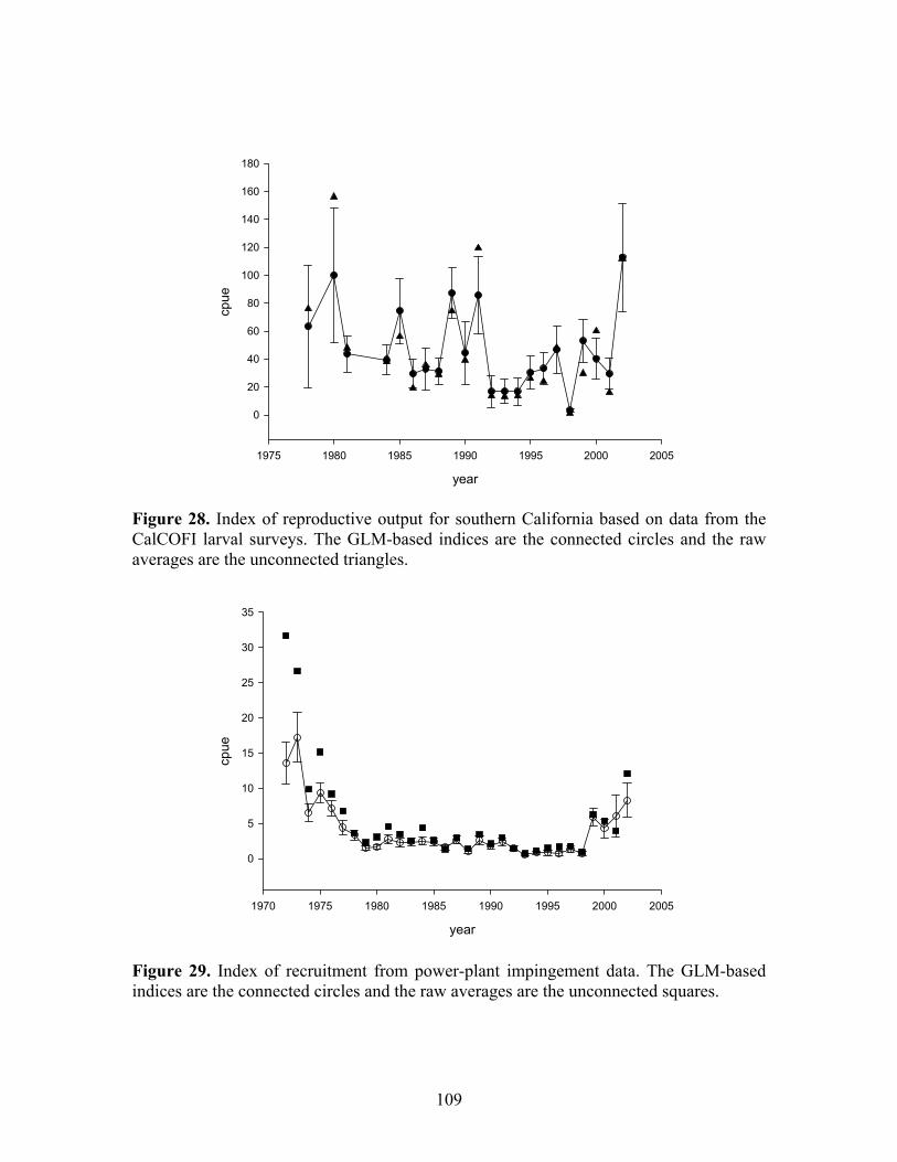
Cal_COFI larval survey

year

1975 1980 1985 1990 1995 2000 2005

cpue

0

20

40

60

80

100

120

140

160

180

Power-Plant CPUE

e

0

5

10

15

20

25

30

35

Figure 28. Index of reproductive output for southern California based on data from the CalCOFI larval surveys. The GLM-based indices are the connected circles and the raw averages are the unconnected triangles.

1970 1975 1

cpu

Figure 29. Index of recruitment indices are the connected circles a

year

980 1985 1990 1995 2000 2005

from power-plant impingement data. The GLM-based nd the raw averages are the unconnected squares.

109

length cm

0 10 20 30 40 50 60 70

prop

ortio

n

0.00

0.05

0.10

0.15

0.20

0.25

Figure 30. The raw length frequency of cabezon sampled in the power plants used to create the impingement time series.

110

1920 1940 1960 1980 2000

050

010

0020

00

Year

Age

0 R

ecru

its (1

000s

)

est. 1916est. 1980

1920 1940 1960 1980 2000

010

020

030

040

0

Year

Age

0 R

ecru

its (1

000s

)

est. 1916est. 1970

Figure 31. Comparison of recruitment trajectories when recruitment estimation begins at the start of the model (1916) or in the year used for the base case for each cabezon substock.

111

1920 1940 1960 1980 2000

0.0

0.5

1.0

1.5

2.0

Year

Std

. Dev

. of R

ecru

itmen

t Dev

s.

1920 1940 1960 1980 2000

0.0

0.5

1.0

1.5

2.0

Year

Std

. Dev

. of R

ecru

itmen

t Dev

s.A) NCS

B) SCS

Figure 32. Asymptotic standard errors for the annual recruitment deviationss for the A) NCS and B) SCS.

112

1920 1940 1960 1980 2000

040

080

012

00

Year

Age

0 R

ecru

its (1

000s

)est. 2004est. 2003est. 2002

1920 1940 1960 1980 2000

010

020

030

040

0

Year

Age

0 R

ecru

its (1

000s

)

est. 2004est. 2003est. 2002

1920 1940 1960 1980 2000

040

080

012

00

Year

Spa

wni

ng B

iom

ass

(in m

t)

est. 2004est. 2003est. 2002

1920 1940 1960 1980 2000

050

150

250

YearS

paw

ning

Bio

mas

s (in

mt)

est. 2004est. 2003est. 2002

1920 1940 1960 1980 2000

040

080

012

00

Year

Age

0 R

ecru

its (1

000s

)est. 2004est. 2003est. 2002

1920 1940 1960 1980 2000

010

020

030

040

0

Year

Age

0 R

ecru

its (1

000s

)

est. 2004est. 2003est. 2002

1920 1940 1960 1980 2000

040

080

012

00

Year

Spa

wni

ng B

iom

ass

(in m

t)

est. 2004est. 2003est. 2002

1920 1940 1960 1980 2000

050

150

250

YearS

paw

ning

Bio

mas

s (in

mt)

est. 2004est. 2003est. 2002

Figure 33. An example of the sensitivity of the time-trajectories of recruitment and spawning biomass to the last year for which recruitment deviations are estimated.

113

114

1960 1970 1980 1990 2000

0.00

0.01

0.02

0.03

0.04

Year

Inde

x va

lue

0.000 0.010 0.020 0.030

0.00

00.

010

0.02

00.

030

Observed

Mod

el p

redi

cted

Figure 34. Fits to CPFV CPUE data for the NCS. The left panel shows the fit of the model (solid red line) to the observed CPUE data (solid black dots). The vertical lines in the left panel are the 95% confidence intervals for the data (based on the assumed coefficients of variation). The panel on the right compares the observed and model-predicted abundance indices, with the solid line indicating the 1:1 relationship.

1960 1970 1980 1990 2000

0.00

00.

002

0.00

40.

006

0.00

8

CPFV

Year

Inde

x va

lue

1980 1990 20000

200

400

600

800

CalCOFI manta tows

Year

Inde

x va

lue

1970 1980 1990 2000

010

2030

4050

6070

Impingement

Year

Inde

x va

lue

0.000 0.002 0.004

0.00

00.

001

0.00

20.

003

0.00

40.

005

Observed

Mod

el p

redi

cted

0 20 40 60 80 100

020

4060

8010

012

0

Observed

Mod

el p

redi

cted

0 5 10 15

05

1015

Observed

Mod

el p

redi

cted

Figure 35. Fits to the abundance indices for the SCS. The upper panels show the fit of the model (solid red lines) to the observed indices (solid black dots). The vertical lines in the upper panels are the 95% confidence intervals for the data (based on the assumed coefficients of variation). The lower panels compare the observed and model-predicted abundance indices, with the solid lines indicating the 1:1 relationships.

115

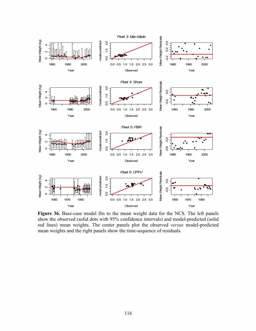
1980 1990 2000

02

4

Year

Mea

n W

eigh

t (kg

)

0.0 0.5 1.0 1.5 2.0 2.5 3.0

0.0

1.5

3.0

Fleet 3: Man Made

Observed

mod

el p

redi

cted

1980 1990 2000

-0.2

0.2

0.5

Year

Mea

n W

eigh

t Res

idua

ls

1960 1980 2000

02

4

Year

Mea

n W

eigh

t (kg

)

0.0 0.5 1.0 1.5 2.0 2.5 3.00.

01.

53.

0

Fleet 4: Shore

Observed

mod

el p

redi

cted

1960 1980 2000

-0.4

0.2

Year

Mea

n W

eigh

t Res

idua

ls

1980 1990 2000

02

4

Year

Mea

n W

eigh

t (kg

)

0.0 0.5 1.0 1.5 2.0 2.5 3.0

0.0

1.5

3.0

Fleet 5: PBR

Observed

mod

el p

redi

cted

1980 1990 2000

-0.8

-0.2

YearM

ean

Wei

ght R

esid

uals

1950 1970 1990

02

4

Year

Mea

n W

eigh

t (kg

)

0.0 0.5 1.0 1.5 2.0 2.5 3.0

0.0

1.5

3.0

Fleet 6: CPFV

Observed

mod

el p

redi

cted

1950 1970 1990

-0.5

0.5

Year

Mea

n W

eigh

t Res

idua

ls

Figure 36. Base-case model fits to the mean weight data for the NCS. The left panels show the observed (solid dots with 95% confidence intervals) and model-predicted (solid red lines) mean weights. The center panels plot the observed versus model-predicted mean weights and the right panels show the time-sequence of residuals.

116

1980 1985 1990 1995 2000

01

23

Year

Mea

n W

eigh

t (kg

)

0.0 0.5 1.0 1.5 2.0 2.5 3.0

0.0

1.5

3.0

Feet 3: Man Made

Observed

mod

el p

redi

cted

1980 1985 1990 1995 2000

-0.1

0.2

Year

Mea

n W

eigh

t Res

idua

ls

1980 1990 2000

0.0

1.5

3.0

Year

Mea

n W

eigh

t (kg

)

0.0 0.5 1.0 1.5 2.0 2.5 3.00.

01.

53.

0

Fleet 4: Shore

Observed

mod

el p

redi

cted

1980 1990 2000

-0.4

0.2

0.8

Year

Mea

n W

eigh

t Res

idua

ls

1980 1990 2000

0.0

1.5

3.0

Year

Mea

n W

eigh

t (kg

)

0.0 0.5 1.0 1.5 2.0 2.5 3.0

0.0

1.5

3.0

Fleet 5: PBR

Observed

mod

el p

redi

cted

1980 1990 2000

-0.6

0.0

0.6

YearM

ean

Wei

ght R

esid

uals

1980 1990 2000

01

23

Year

Mea

n W

eigh

t (kg

)

0.0 0.5 1.0 1.5 2.0 2.5 3.0

0.0

1.5

3.0

Fleet 6: CPFV

Observed

mod

el p

redi

cted

1980 1990 2000

0.0

1.0

Year

Mea

n W

eigh

t Res

idua

ls

Figure 37. Base-case model fits to the mean weight data for the SCS. The left panels show the observed (solid dots with 95% confidence intervals) and model-predicted (solid red lines) mean weights. The center panels plot the observed versus model-predicted mean weights and the right panels show the time-sequence of residuals.

117

30 40 50 60

0.00

0.04

0.08

1995

Length (cm)

Prop

ortio

ns a

t Len

gth

20 30 40 50 60

0.0

0.2

0.4

1996

Length (cm)

Prop

ortio

ns a

t Len

gth

30 40 50 60

0.0

0.2

0.4

1997

Length (cm)

Prop

ortio

ns a

t Len

gth

25 30 35 40 45 50

0.0

0.2

0.4

1998

Length (cm)

Prop

ortio

ns a

t Len

gth

35 40 45 50

0.0

0.2

0.4

1999

Length (cm)

Prop

ortio

ns a

t Len

gth

35 40 45 50 55 60 65

0.0

0.2

0.4

2000

Length (cm)

Prop

ortio

ns a

t Len

gth

1995 1997 1999

Year

Effe

ctiv

e sa

mpl

e si

ze

050

010

0015

00

0 500 1000 1500

050

010

00

Input Sample Size

Effe

ctiv

e Sa

mpl

e Si

ze

Figure 38. Observed (solid circles) and model-predicted (solid lines) length-composition data for the commercial non-live-fish fleet (fleet 1) in the NCS. The annual effective sample sizes are summarized by the histogram and a comparison of inputted to effective sample sizes is given in the lower center panel (the solid red line in this panel is the 1:1 line).

118

35 40 45 50 55 60

0.00

0.10

0.20

1997

Length (cm)

Prop

ortio

ns a

t Len

gth

25 30 35 40 45 50 55 60

0.0

0.2

0.4

1998

Length (cm)

Prop

ortio

ns a

t Len

gth

30 40 50 60

0.0

0.2

0.4

1999

Length (cm)

Prop

ortio

ns a

t Len

gth

30 40 50 60

0.0

0.2

0.4

2000

Length (cm)

Prop

ortio

ns a

t Len

gth

35 40 45 50 55 60 65

0.0

0.2

0.4

2001

Length (cm)

Prop

ortio

ns a

t Len

gth

35 40 45 50 55 60 65

0.0

0.2

0.4

2002

Length (cm)

Prop

ortio

ns a

t Len

gth

1997 1999 2001 2003

Year

Effe

ctiv

e sa

mpl

e si

ze

010

020

030

0

0 100 200 300

010

020

030

0

Input Sample Size

Effe

ctiv

e Sa

mpl

e Si

ze

Figure 39. Observed (solid circles) and model-predicted (solid lines) length-composition data for the commercial live-fish fleet (fleet 2) in the NCS. The annual effective sample sizes are summarized by the histogram and a comparison of inputted to effective sample sizes is given in the lower center panel (the solid red line in this panel is the 1:1 line).

119

20 30 40 50

0.00

0.10

1993

Length (cm)

Prop

ortio

ns a

t Len

gth

20 30 40 50

0.0

0.2

0.4

1994

Length (cm)

Prop

ortio

ns a

t Len

gth

20 30 40 50 60

0.0

0.2

0.4

1995

Length (cm)

Prop

ortio

ns a

t Len

gth

25 35 45

0.0

0.2

0.4

1996

Length (cm)

Prop

ortio

ns a

t Len

gth

25 30 35 40

0.0

0.2

0.4

1997

Length (cm)

Prop

ortio

ns a

t Len

gth

25 35 45

0.0

0.2

0.4

1998

Length (cm)

Prop

ortio

ns a

t Len

gth

25 30 35 40

0.0

0.2

0.4

1999

Length (cm)

Prop

ortio

ns a

t Len

gth

34 36 38 40

0.0

0.2

0.4

2000

Length (cm)

Prop

ortio

ns a

t Len

gth

25 30 35 40

0.0

0.2

0.4

2001

Length (cm)

Prop

ortio

ns a

t Len

gth

20 30 40 50

0.0

0.2

0.4

2002

Length (cm)

Prop

ortio

ns a

t Len

gth

30 35 40 45

0.0

0.2

0.4

2003

Length (cm)

Prop

ortio

ns a

t Len

gth

30 40 50

0.0

0.2

0.4

2004

Length (cm)

Prop

ortio

ns a

t Len

gth

1993 1998 2003

Year

Effe

ctiv

e sa

mpl

e si

ze

020

40

0 20 40

020

40

Input Sample Size

Effe

ctiv

e Sa

mpl

e Si

ze

Figure 40. Observed (solid circles) and model-predicted (solid lines) length-composition data for the recreational shore mode (fleet 4) in the NCS. The annual effective sample sizes are summarized by the histogram and a comparison of inputted to effective sample sizes is given in the lower center panel (the solid red line in this panel is the 1:1 line).

120

20 30 40 50 60

0.00

0.06

1993

Length (cm)

Prop

ortio

ns a

t Len

gth

30 40 50 60

0.0

0.2

0.4

1994

Length (cm)

Prop

ortio

ns a

t Len

gth

30 40 50 60

0.0

0.2

0.4

1995

Length (cm)

Prop

ortio

ns a

t Len

gth

30 40 50 60

0.0

0.2

0.4

1996

Length (cm)

Prop

ortio

ns a

t Len

gth

38 40 42 44 46

0.0

0.2

0.4

1997

Length (cm)

Prop

ortio

ns a

t Len

gth

20 30 40 50

0.0

0.2

0.4

1998

Length (cm)

Prop

ortio

ns a

t Len

gth

35 40 45 50

0.0

0.2

0.4

1999

Length (cm)

Prop

ortio

ns a

t Len

gth

35 45 55

0.0

0.2

0.4

2000

Length (cm)

Prop

ortio

ns a

t Len

gth

25 35 45 55

0.0

0.2

0.4

2001

Length (cm)

Prop

ortio

ns a

t Len

gth

30 40 50 60

0.0

0.2

0.4

2002

Length (cm)

Prop

ortio

ns a

t Len

gth

10 30 50

0.0

0.2

0.4

2003

Length (cm)

Prop

ortio

ns a

t Len

gth

30 40 50 60

0.0

0.2

0.4

2004

Length (cm)

Prop

ortio

ns a

t Len

gth

1993 1998 2003

Year

Effe

ctiv

e sa

mpl

e si

ze

040

100

0 40 80 120

040

100

Input Sample Size

Effe

ctiv

e Sa

mpl

e Si

ze

Figure 41. Observed (solid circles) and model-predicted (solid lines) length-composition data for the recreational PBR mode (fleet 5) in the NCS. The annual effective sample sizes are summarized by the histogram and a comparison of inputted to effective sample sizes is given in the lower center panel (the solid red line in this panel is the 1:1 line).

121

35 45 55

0.02

0.08

1987

Length (cm)

Prop

ortio

ns a

t Len

gth

30 40 50 60

0.0

0.2

0.4

1988

Length (cm)

Prop

ortio

ns a

t Len

gth

30 40 50 60

0.0

0.2

0.4

1989

Length (cm)

Prop

ortio

ns a

t Len

gth

35 45 55

0.0

0.2

0.4

1990

Length (cm)

Prop

ortio

ns a

t Len

gth

40 45 50 55

0.0

0.2

0.4

1991

Length (cm)

Prop

ortio

ns a

t Len

gth

35 45 55

0.0

0.2

0.4

1992

Length (cm)

Prop

ortio

ns a

t Len

gth

35 45 55

0.0

0.2

0.4

1993

Length (cm)

Prop

ortio

ns a

t Len

gth

30 40 50 60

0.0

0.2

0.4

1994

Length (cm)

Prop

ortio

ns a

t Len

gth

30 40 50

0.0

0.2

0.4

1995

Length (cm)

Prop

ortio

ns a

t Len

gth

30 40 50 60

0.0

0.2

0.4

1996

Length (cm)

Prop

ortio

ns a

t Len

gth

25 35 45 55

0.0

0.2

0.4

1997

Length (cm)

Prop

ortio

ns a

t Len

gth

30 40 50

0.0

0.2

0.4

1998

Length (cm)

Prop

ortio

ns a

t Len

gth

1987 1992 1997

Year

Effe

ctiv

e sa

mpl

e si

ze

040

80

0 20 60 100

040

80

Input Sample Size

Effe

ctiv

e Sa

mpl

e Si

ze

Figure 42. Observed (solid circles) and model-predicted (solid lines) length-composition data for the recreational CPFV mode (fleet 6) in the NCS from CDF&G observer data. The annual effective sample sizes are summarized by the histogram and a comparison of inputted to effective sample sizes is given in the lower center panel (the solid red line in this panel is the 1:1 line).

122

30 40 50 60 70

0.00

0.04

0.08

1996

Length (cm)

Prop

ortio

ns a

t Len

gth

25 30 35 40 45 50

0.0

0.2

0.4

1997

Length (cm)

Prop

ortio

ns a

t Len

gth

25 30 35 40 45 50

0.0

0.2

0.4

1998

Length (cm)

Prop

ortio

ns a

t Len

gth

35 40 45 50 55

0.0

0.2

0.4

2001

Length (cm)

Prop

ortio

ns a

t Len

gth

35 40 45 50 55 60 65 70

0.0

0.2

0.4

2003

Length (cm)

Prop

ortio

ns a

t Len

gth

30 40 50 60

0.0

0.2

0.4

2004

Length (cm)

Prop

ortio

ns a

t Len

gth

1996 1998 2003

Year

Effe

ctiv

e sa

mpl

e si

ze

05

1525

35

0 5 10 15 20 25 30 35

05

1525

35

Input Sample Size

Effe

ctiv

e Sa

mpl

e Si

ze

Figure 43. Observed (solid circles) and model-predicted (solid lines) length-composition data for the recreational CPFV mode (fleet 6) in the NCS from RecFIN. The annual effective sample sizes are summarized by the histogram and a comparison of inputted to effective sample sizes is given in the lower center panel (the solid red line in this panel is the 1:1 line).

123

Ye

ar

Figucomreprand

A) NCS Fleet 1: Commercial non-live
20 22 24 26 28 30 32 34 36 38 40 42 44 46 48 50 52 54 56 58 60 62 64 66
199519961997199819992000
B) NCS Fleet 2: Commercial live-fish
24 26 28 30 32 34 36 38 40 42 44 46 48 50 52 54 56 58 60 62 6419971998199920002001200220032004

Length Bin

14 16 18 20 22 24 26 28 30 32 34 36 38 40 42 44 46 48 50 52 54 56 58 60 62199319941995199619971998199920002001200220032004

C) NCS Fleet 4: Recreational Shore

re 44. Pearson residual plots of fits to the length-composition data for the mercial fleets (A and B) and the recreational shore fleet in the NCS. Solid symbols esent negative values; open symbols positive values; squares represent residuals <-2 >2.

124

6 8 10 12 14 16 18 20 22 24 26 28 30 32 34 36 38 40 42 44 46 48 50 52 54 56 58 60 62 64 66 68199319941995199619971998199920002001200220032004

Year

22 24 26 28 30 32 34 36 38 40 42 44 46 48 50 52 54 56 58 60 62 64 66198719881989199019911992199319941995199619971998

Length Bin

24 26 28 30 32 34 36 38 40 42 44 46 48 50 52 54 56 58 60 62 64 66 68 70 72199619971998200120032004

A) NCS Fleet 5: Recreational PBR

B) NCS Fleet 6: Recreational CPFV (Observer)

C) NCS Fleet 6: Recreational CPFV (RecFIN)

Figure 45. Pearson residual plots of fits to length composition data for the recreational fleets in the NCS. Solid symbols represent negative values; open symbols positive values; squares represent residuals <-2 and >2.

125

30 35 40 45 50 55 60

0.00

0.04

0.08

0.12

1994

Length (cm)

Prop

ortio

ns a

t Len

gth

30 40 50 60

0.0

0.2

0.4

1996

Length (cm)

Prop

ortio

ns a

t Len

gth

30 35 40

0.0

0.2

0.4

1998

Length (cm)

Prop

ortio

ns a

t Len

gth

20 25 30 35 40 45 50

0.0

0.2

0.4

1999

Length (cm)

Prop

ortio

ns a

t Len

gth

30 35 40 45 50

0.0

0.2

0.4

2002

Length (cm)

Prop

ortio

ns a

t Len

gth

30 35 40 45 50

0.0

0.2

0.4

2003

Length (cm)

Prop

ortio

ns a

t Len

gth

30 40 50 60

0.0

0.2

0.4

2004

Length (cm)

Prop

ortio

ns a

t Len

gth

1994 1998 2002 2004

Year

Effe

ctiv

e sa

mpl

e si

ze

010

2030

4050

0 10 20 30 40 50

010

2030

4050

Input Sample Size

Effe

ctiv

e Sa

mpl

e Si

ze

Figure 46. Observed (solid circles) and model-predicted (solid lines) length-composition data for the recreational PBR mode (fleet 5) in the SCS. The annual effective sample sizes are summarized by the histogram and a comparison of inputted to effective sample sizes is given in the lower center panel (the solid red line in this panel is the 1:1 line).

126

20 30 40 50

0.02

0.06

0.10

1975

Length (cm)

Prop

ortio

ns a

t Len

gth

20 30 40 50

0.0

0.2

0.4

1976

Length (cm)Pr

opor

tions

at L

engt

h

20 40 60

0.0

0.2

0.4

1977

Length (cm)

Prop

ortio

ns a

t Len

gth

20 40

0.0

0.2

0.4

1978

Length (cm)

Prop

ortio

ns a

t Len

gth

20 30 40

0.0

0.2

0.4

1986

Length (cm)

Prop

ortio

ns a

t Len

gth

25 30 35 40

0.0

0.2

0.4

1987

Length (cm)

Prop

ortio

ns a

t Len

gth

25 35 450.

00.

20.

4

1988

Length (cm)

Prop

ortio

ns a

t Len

gth

15 25 35 45

0.0

0.2

0.4

1989

Length (cm)

Prop

ortio

ns a

t Len

gth

1975 1978 1988

Year

Effe

ctiv

e sa

mpl

e si

ze

040

8012

0

0 50 100

050

100

Input Sample Size

Effe

ctiv

e Sa

mpl

e Si

ze

Figure 47. Observed (solid circles) and model-predicted (solid lines) length-composition data for the recreational CPFV mode (fleet 6) in the SCS from CDF&G observer data. The annual effective sample sizes are summarized by the histogram and a comparison of inputted to effective sample sizes is given in the lower center panel (the solid red line in this panel is the 1:1 line).

127

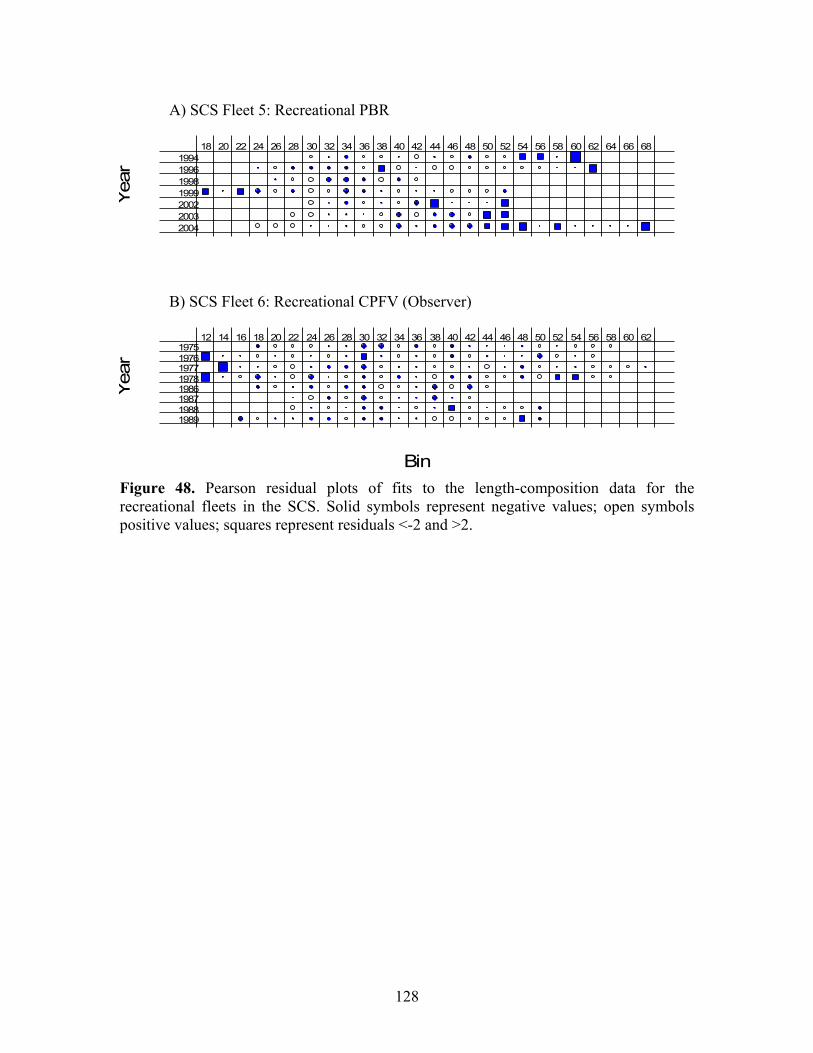
Yea

r18 20 22 24 26 28 30 32 34 36 38 40 42 44 46 48 50 52 54 56 58 60 62 64 66 68

1994199619981999200220032004

Bin

Yea

r

12 14 16 18 20 22 24 26 28 30 32 34 36 38 40 42 44 46 48 50 52 54 56 58 60 6219751976197719781986198719881989

A) SCS Fleet 5: Recreational PBR

B) SCS Fleet 6: Recreational CPFV (Observer)

Figure 48. Pearson residual plots of fits to the length-composition data for the recreational fleets in the SCS. Solid symbols represent negative values; open symbols positive values; squares represent residuals <-2 and >2.

128

A) Reproductive Output

1920 1940 1960 1980 2000

050

010

0015

00

Year

Spa

wning

Biomass (m

t)

B) Recruitment

1920 1940 1960 1980 2000

050

010

0015

0020

00

Year

Rec

ruits (1

000s

)

Figure 49. MPD time-trajectories of A) reproductive output (measured in spawning biomass) and B) recruitment for the NCS. The vertical bars represent asymptotic 95% confidence intervals.

129

A) NCS

0 200 400 600 800 1000

050

010

0015

00

Spawning Biomass (mt)

Rec

ruits

(100

0s)

Expected Mean RecruitsBias-adjusted Expected Recruits

50 100 150 200 250

010

030

050

0

Spawning Biomass (mt)

Rec

ruits

(100

0s)

Expected Mean RecruitsBias-adjusted Expected Recruits

B) SCS

Figure 50. Relationship between spawners and recruits for A) the NCS and B) the SCS.

130

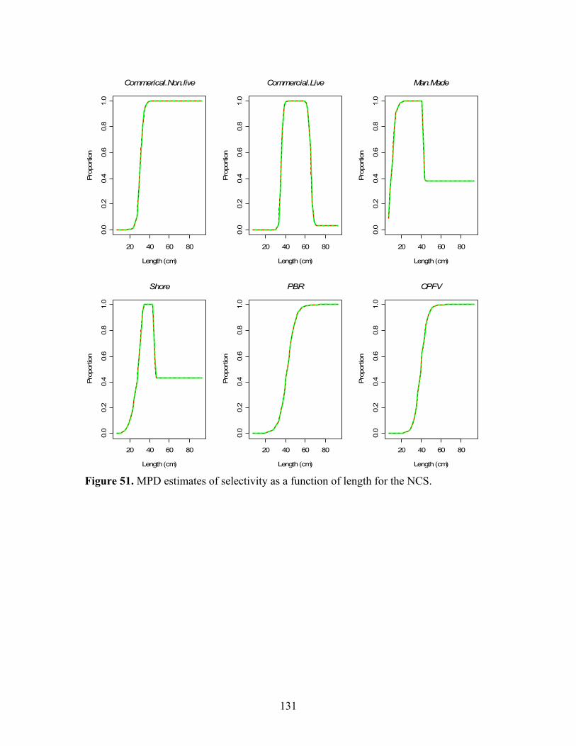
20 40 60 80

0.0

0.2

0.4

0.6

0.8

1.0

Commerical.Non.live

Length (cm)

Prop

ortio

n

20 40 60 800.

00.

20.

40.

60.

81.

0

Commercial.Live

Length (cm)

Prop

ortio

n

20 40 60 80

0.0

0.2

0.4

0.6

0.8

1.0

Shore

Length (cm)

Prop

ortio

n

20 40 60 80

0.0

0.2

0.4

0.6

0.8

1.0

PBR

Length (cm)

Prop

ortio

n

20 40 60 80

0.0

0.2

0.4

0.6

0.8

1.0

Man.Made

Length (cm)

Prop

ortio

n

20 40 60 80

0.0

0.2

0.4

0.6

0.8

1.0

CPFV

Length (cm)

Prop

ortio

n

Figure 51. MPD estimates of selectivity as a function of length for the NCS.

131

0 5 10 15 20 25 30 35

0.0

0.2

0.4

0.6

0.8

1.0

Commerical.Non.live

Age (yr)

Prop

ortio

n

0 5 10 15 20 25 30 350.

00.

20.

40.

60.

81.

0

Commercial.Live

Age (yr)

Prop

ortio

n

0 5 10 15 20 25 30 35

0.0

0.2

0.4

0.6

0.8

1.0

Man.Made

Age (yr)

Prop

ortio

n

0 5 10 15 20 25 30 35

0.0

0.2

0.4

0.6

0.8

1.0

Shore

Age (yr)

Prop

ortio

n

0 5 10 15 20 25 30 35

0.0

0.2

0.4

0.6

0.8

1.0

PBR

Age (yr)

Prop

ortio

n

0 5 10 15 20 25 30 35

0.0

0.2

0.4

0.6

0.8

1.0

CPFV

Age (yr)

Prop

ortio

n

Figure 52. MPD estimates of selectivity as a function of age for the NCS (females: solid lines; males: dashed lines).

132

1920 1940 1960 1980 2000

0.00

00.

005

0.01

00.

015

0.02

00.

025

Commerical: Non-live

Year

Har

vest

rate

1920 1940 1960 1980 20000.

000.

050.

100.

150.

20

Commerical: Live

Year

Har

vest

rate

1920 1940 1960 1980 2000

0.00

00.

005

0.01

00.

015

Recreational: Man-made

Year

Har

vest

rate

1920 1940 1960 1980 2000

0.00

0.01

0.02

0.03

0.04

0.05

Recreational: Shore

Year

Har

vest

rate

1920 1940 1960 1980 2000

0.00

0.05

0.10

0.15

Recreational: PBR

Year

Har

vest

rate

1920 1940 1960 1980 2000

0.00

0.01

0.02

0.03

Recreational: CPFV

Year

Har

vest

rate

Figure 53. MPD estimates of harvest rate by fleet for the NCS.

133

A) Reproductive Output

1920 1940 1960 1980 2000

050

100

150

200

250

300

Year

Spa

wning

Biomas

s (m

t)

020

040

060

080

0

Year

Recruits (1

000s)

B) Recruitment

1920 1940 1960 1980 2000

Figure 54. MPD time-trajectories of A) reproductive output (measured in spawning biomass (mt)) and B) recruitment (1000s) for the SCS. The vertical bars represent asymptotic 95% confidence intervals.

134

20 40 60 80

0.0

0.2

0.4

0.6

0.8

1.0

Commerical.Non.live

Length (cm)

Prop

ortio

n

20 40 60 80

0.0

0.2

0.4

0.6

0.8

1.0

Commercial.Live

Length (cm)

Prop

ortio

n

20 40 60 80

0.0

0.2

0.4

0.6

0.8

1.0

Man.Made

Length (cm)

Prop

ortio

n

20 40 60 80

0.0

0.2

0.4

0.6

0.8

1.0

Shore

Length (cm)

Prop

ortio

n

20 40 60 80

0.0

0.2

0.4

0.6

0.8

1.0

PBR

Length (cm)

Prop

ortio

n

20 40 60 80

0.0

0.2

0.4

0.6

0.8

1.0

CPFV

Length (cm)

Prop

ortio

n

Figure 55. MPD estimates of selectivity as a function of length for the SCS.

135

0 5 10 15 20 25 30 35

0.0

0.2

0.4

0.6

0.8

1.0

Commerical.Non.live

Age (yr)

Prop

ortio

n

0 5 10 15 20 25 30 350.

00.

20.

40.

60.

81.

0

Commercial.Live

Age (yr)

Prop

ortio

n

0 5 10 15 20 25 30 35

0.0

0.2

0.4

0.6

0.8

1.0

Man.Made

Age (yr)

Prop

ortio

n

0 5 10 15 20 25 30 35

0.0

0.2

0.4

0.6

0.8

1.0

Shore

Age (yr)

Prop

ortio

n

0 5 10 15 20 25 30 35

0.0

0.2

0.4

0.6

0.8

1.0

PBR

Age (yr)

Prop

ortio

n

0 5 10 15 20 25 30 35

0.0

0.2

0.4

0.6

0.8

1.0

CPFV

Age (yr)

Prop

ortio

n

Figure 56. MPD estimates of selectivity as a function of age for the SCS (females: solid lines; males: dashed lines).

136

1920 1940 1960 1980 2000

0.00

00.

005

0.01

00.

015

Commerical: Non-live

Year

Har

vest

rate

1920 1940 1960 1980 20000.

00.

10.

20.

30.

40.

5

Commerical: Live

Year

Har

vest

rate

1920 1940 1960 1980 2000

0.00

00.

005

0.01

00.

015

0.02

0

Recreational: Man-made

Year

Har

vest

rate

1920 1940 1960 1980 2000

0.00

0.05

0.10

0.15

Recreational: Shore

Year

Har

vest

rate

1920 1940 1960 1980 2000

0.0

0.1

0.2

0.3

0.4

0.5

Recreational: PBR

Year

Har

vest

rate

1920 1940 1960 1980 2000

0.00

0.01

0.02

0.03

0.04

Recreational: CPFV

Year

Har

vest

rate

Figure 57. MPD estimates of harvest rate by fleet for the SCS.

137

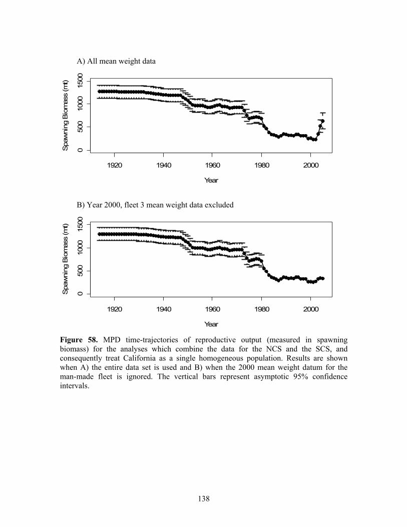
1920 1940 1960 1980 2000

050

010

0015

00

Year

Spa

wni

ng B

iom

ass

(mt)

1920 1940 1960 1980 2000

050

010

0015

00

Year

Spa

wni

ng B

iom

ass

(mt)

A) All mean weight data

B) Year 2000, fleet 3 mean weight data excluded

Figure 58. MPD time-trajectories of reproductive output (measured in spawning biomass) for the analyses which combine the data for the NCS and the SCS, and consequently treat California as a single homogeneous population. Results are shown when A) the entire data set is used and B) when the 2000 mean weight datum for the man-made fleet is ignored. The vertical bars represent asymptotic 95% confidence intervals.

138

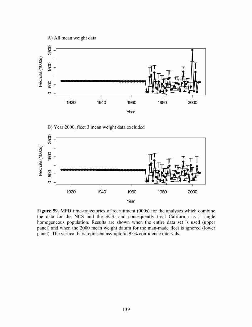
A) All mean weight data

1920 1940 1960 1980 2000

050

015

0025

00

Year

Rec

ruits

(100

0s)

1920 1940 1960 1980 2000

050

015

0025

00

Year

Rec

ruits

(100

0s)

B) Year 2000, fleet 3 mean weight data excluded

Figure 59. MPD time-trajectories of recruitment (000s) for the analyses which combine the data for the NCS and the SCS, and consequently treat California as a single homogeneous population. Results are shown when the entire data set is used (upper panel) and when the 2000 mean weight datum for the man-made fleet is ignored (lower panel). The vertical bars represent asymptotic 95% confidence intervals.

139

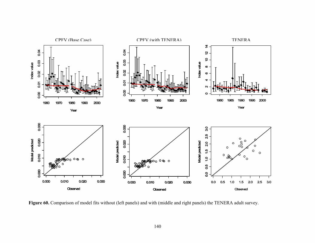
140

1960 1970 1980 1990 2000

0.00

0.01

0.02

0.03

0.04

Year

Inde

x va

lue

02

46

810

1214

Inde

x va

lue

0.000 0.010 0.020 0.030

0.00

00.

010

0.02

00.

030

Observed

Mod

el p

redi

cted

0.0

0.5

1.0

1.5

2.0

2.5

3.0

Mod

el p

redi

cted

1960 1970 1980 1990 2000

0.00

0.01

0.02

0.03

0.04

Year

Inde

x va

lue

0.000 0.010 0.020 0.030

0.00

00.

010

0.02

00.

030

Observed

Mod

el p

redi

cted

1960 1970 1980 1990 2000

0.00

0.01

0.02

0.03

0.04

Year

Inde

x va

lue

02

46

810

1214

Inde

x va

lue

0.000 0.010 0.020 0.030

0.00

00.

010

0.02

00.

030

Observed

Mod

el p

redi

cted

0.0

0.5

1.0

1.5

2.0

2.5

3.0

Mod

el p

redi

cted

1960 1970 1980 1990 2000

0.00

0.01

0.02

0.03

0.04

Year

Inde

x va

lue

0.000 0.010 0.020 0.030

0.00

00.

010

0.02

00.

030

Observed

Mod

el p

redi

cted

Figure 60. Comparison of model fits without (left panels) and with (middle and right panels) th

CPFV (with TENERA)CPFV (Base Case)

0.0 0.5 1.0 1.5 2.0 2.5 3.0

Observed

0.0 0.5 1.0 1.5 2.0 2.5 3.0

Observed

TENERA

1980 1985 1990 1995 2000

Year

1980 1985 1990 1995 2000

Year

e TENERA adult survey.

141

1920 1940 1960 1980 2000

5015

025

0

Year

All datano 2000 Fleet 3 data

1920 1940 1960 1980 2000

010

030

0

Year

All datano 2000 Fleet 3 data

Spa

wni

ng B

iom

ass

(mt)

Rec

ruits

(100

0s)

Figure 61. MPD time-trajectories of reproductive output (upper panel) and recruitment (lower panel) for the SCS. Results are shown when the entire data set is used (“all data”) and when the 2000 mean weight datum for the man-made fleet is ignored (“no 2000 fleet 3 data”). Fleet 3 is the man-made fleet for the SCS.

142

A) Base Case

20 30 40 50

0.0

0.2

0.4

1999

Length (cm)

Prop

ortio

ns a

t Len

gth

30 35 40 45 50

0.0

0.2

0.4

2002

Length (cm)

Prop

ortio

ns a

t Len

gth

30 40 50

0.0

0.2

0.4

2003

Length (cm)

Prop

ortio

ns a

t Len

gth

30 40 50 60

0.0

0.2

0.4

2004

Length (cm)

Prop

ortio

ns a

t Len

gth

20 30 40 50

0.0

0.2

0.4

1999

Length (cm)

Prop

ortio

ns a

t Len

gth

30 35 40 45 50

0.0

0.2

0.4

2002

Length (cm)

Prop

ortio

ns a

t Len

gth

30 40 50

0.0

0.2

0.4

2003

Length (cm)

Prop

ortio

ns a

t Len

gth

30 40 50 60

0.0

0.2

0.4

2004

Length (cm)

Prop

ortio

ns a

t Len

gth

Figure 62. Comparison of fits to the recreational PBR length data when the year 2000 mean weight datum A) is included; B) is not included. A noticeable cohort (following the length modes) is apparent in years 2002-2004.

B) Less 2000 mean weight data for fleet 3 (man-made)

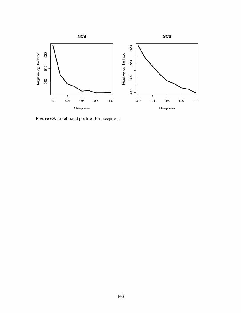
143

0.2 0.4 0.6 0.8 1.0

510

515

520

NCSN

egat

ive

log

likel

ihoo

d

Steepness Figure 63. Likelihood profiles for steepness.

0.2 0.4 0.6 0.8 1.0

300

340

380

420

SCS

g lik

elih

ood

Steepness

Neg

ativ

e lo

0.3 0.5 0.7 0.9

1100

1200

1300

1400

1500

Steepness

Spaw

ning

Bio

mas

s in

191

6

0.3 0.5 0.7 0.938

040

042

044

046

0

NCS

Spaw

ning

Bio

mas

s in

200

5

Steepness

0.3 0.5 0.7 0.9

0.25

0.30

0.35

0.40

0.45

Steepness

Dep

letio

n

0.2 0.4 0.6 0.8 1.0

250

300

350

Steepness

Spaw

ning

Bio

mas

s in

191

6

0.2 0.4 0.6 0.8 1.0

7072

7476

78

SCS

Steepness

Spaw

ning

Bio

mas

s in

200

5

0.2 0.4 0.6 0.8 1.0

0.22

0.24

0.26

0.28

0.30

0.32

Steepness

Dep

letio

n

Figure 64. Beginning (1916) and ending (2005) spawning biomass and depletion for each steepness value in the likelihood profile. Base case value: steepness = 0.7. Note the limited range of the y-axes make the local minimums (kinks) distinct.

144

1920 1940 1960 1980 2000

050

010

0015

00

NCS

Year

SCS

Base Case95% CIHigh MLow M

1920 1940 1960 1980 2000

050

100

200

300

Year

Spa

wni

ng B

iom

ass

(mt)

Base Case95% CILow depletionHigh depletion

1920 1940 1960 1980 2000

050

010

0015

0020

00

Year

Base Case95% CIHigh MLow M

1920 1940 1960 1980 2000

010

030

050

0

Year

Rec

ruitm

ent (

1000

s)

Base Case95% CILow depletionHigh depletion

t)

s (m

omas

i

ning

B

paw

S

)

000s

(1

men

t

crui

t

Re

Figure 65. Spawning biomass (upper panels) and recruitement trajectories (lower panels) for the NCS (left panels) and SCS (right panels) under different states of nature. For the NSC, low and high M states refer to natural mortality values of 0.2/0.25 and 0.3/0.35 for females and males respectively. For the SCS, low depletion and high depletion states refer to depletions of 20% and 35% at the start of year 2000 respectivley.

145

Appendix A. Summary of California Management Measures Affecting Cabezon Year Description Effective Date 1982 Recreational and commercial size limit 12" total length 1/1/1982 1999 Recreational and commercial size limit 14" total length 1/1/1999 Pre-2000 Recreational Bag Limit of 10 fish w/in 20 fish aggregate 3/1/1984 2000 FGC fixes cabezon OY at 67,132 pounds (37.6%)

recreational; 111,596 pounds (62.4%) commercial; Total = 178,728 pounds

10/2000

2000 FGC changes cabezon OY to 63,608 pounds (40.3%) recreational; 94,398 pounds (59.7%) commercial; Total = 158,006 pounds

12/2000

2001 Weekday closures - Commercial take prohibited Thursday through Sunday

01/2001

2001 Central and Southern Management Areas; recreational bag limit 10 fish; Recreational Fishery open year round; no depth restrictions, except no take in Cowcod Closure area in southern management area

1/1/2001

2001 Size limit increased to 15" total length (recreational and commercial)

Mar-01

2001 FGC fixes cabezon OY at 63,608 pounds recreational; 94,398 pounds commercial; Total OY = 178,728 pounds in emergency regulations

Sep-01

2002 Finfish traps required to have rigid 5” rings in entrance 1/8/2002

2002 FGC fixes cabezon OY at 84,330 pounds (47.2%) recreational; 94,398 (52.8%) pounds commercial; Total OY = 178,728 pounds reaffirming emergency action

2/4/2002

2003 Northern Rockfish and Lingcod Management Area; recreational bag limit remains at 10 fish; Open year round; No depth Restriction

1/3/2003

2003 FGC fixes cabezon OY at 118,300 pounds (61%) recreational; 75,600 pounds (39%) commercial; Total OY = 193,900 pounds

1/1/2004

2004 FGC fixes cabezon OY at 92,793 pounds (61%) recreational; 59,326 pounds (39%) commercial; Total OY = 152119 pounds

1/1/2004

2004 Recreational rockfish, cabezon, and greenling (RCG) complex; 10 fish bag-limit regulation established; cabezon sub-limit 3 fish/bag limit

5/1/2004

146

Appendix B-1. SS2 .DAT File for the NCS

#_Number_of_datafiles: 1 #_start_nudata: 1 1916 #_styr 2004 #_endyr 1 #N_seasons_per_year 12 #vector_with_N_months_in_each_season 1 #spawning_season_-_spawning_will_occur_at_beginning_of_this_season 6 #N_fishing_fleets 1 #N_surveys;_data_type_numbers_below_must_be_sequential_with_the_N_fisheries fleet1%fleet2%fleet3%fleet4%fleet5%fleet6%survey1 0.5 0.5 0.5 0.5 0.5 0.5 0.5 #_surveytiming_in_season 2 #number_of_genders(1 / 2) 35 #accumulator_age;_model_always_starts_with_age_0 #Catch (mt) #Fleet 1 #Fleet 2 #Fleet 3 #Fleet 4 #Fleet 5 #Fleet 6 #Comm NCAL #NCAL_live #N_Man-made #N_Shore #N_PBR #N_CPFV #Year 0 0 0 0 0 0 # initial_equilibrium 0.031751462 0 0.329896077 0.707217857 0 0 #1916 1 0.151499831 0 0.329896077 0.707217857 0 0 #1917 1 0.075749916 0 0.329896077 0.707217857 0 0 #1918 1 0 0 0.329896077 0.707217857 0 0 # 1919 1 0 0 0.329896077 0.707217857 0 0 # 1920 1 0 0 0.329896077 0.707217857 0 0 # 1921 1 0 0 0.329896077 0.707217857 0 0 # 1922 1 0 0 0.329896077 0.707217857 0 0 # 1923 1 0 0 0.329896077 0.707217857 0 0 # 1924 1 1.520441422 0 0.329896077 0.707217857 0 0 #1925 1 0 0 0.329896077 0.707217857 0 0 # 1926 1 0.341101417 0 0.329896077 0.707217857 0 0 #1927 1 1.19204059 0 0.329896077 0.707217857 0 0 #1928 1 0.542496402 0 0.329896077 0.707217857 0.489879695 0.979759389 #1929 0.474457556 0 0.494080468 1.059189707 0.733685561 1.467371122 #1930 0.505301833 0 0.658264858 1.411161557 0.977491428 1.954982855 #1931 2.12099764 0 0.8216856 1.761496329 1.220163313 2.440326626 #1932 1.901458962 0 0.985869991 2.113468179 1.46396918 2.927938359 #1933 2.369566226 0 1.150054381 2.46544003 1.707775046 3.415550092 #1934 4.712370506 0 1.314238772 2.81741188 1.951580913 3.903161825 #1935 8.334305099 0 1.846501656 3.958455506 2.741965512 5.483931025 #1936 3.713106648 0 1.595261356 3.419856721 2.368885838 4.737771675 #1937 2.460284688 0 3.05001142 6.538491021 4.529119213 9.058238426 #1938 1.823441085 0 1.735009 3.719442063 2.576404319 5.152808639 #1939 1.511823168 0 2.533785151 5.431826041 3.762548209 7.525096419 #1940 6.018262766 0 1.927448379 5.164982267 0 5.724334949 #1941 1.039633574 0 1.927448379 5.164982267 0 5.724334949 #1942 3.410560577 0 1.927448379 5.164982267 0 5.724334949 #1943 1.754041462 0 1.927448379 5.164982267 0 5.724334949 #1944 1.951807709 0 1.927448379 5.164982267 0 5.724334949 #1945 3.542102347 0 1.927448379 5.164982267 0 5.724334949 #1946 2.046608502 0 7.649465297 20.49826758 11.35908542 22.71817083 #1947 3.714467425 0 10.24586961 27.45585066 15.21462005 30.4292401 #1948 7.273352687 0 9.376074166 25.12506033 13.92301595 27.8460319 #1949 9.544035789 0 10.76896872 28.85759902 15.99139688 31.98279376 #1950

147

10.80230086 0 12.75674531 34.18424277 18.94314884 37.88629767 #1951 15.59541079 0 6.649085988 17.81755174 9.873570602 19.7471412 #1952 6.02098432 0 4.678873303 12.53797399 6.947900205 13.89580041 #1953 2.816354651 0 3.483000022 9.333393074 5.172086312 10.34417262 #1954 3.141126745 0 3.09583032 8.295894655 9.194316119 9.194316119 #1955 5.565577641 0 6.779669852 18.16747724 20.13496263 20.13496263 #1956 5.626812602 0 6.064131369 16.2500492 18.00988266 18.00988266 #1957 8.787443817 0 4.17792 11.48042136 12.40801763 12.40801763 #1958 1 4.29687995 0 3.324924818 14.9684624 9.874704583 9.874704583 #1959 1.385270914 0 1.558606237 11.48042136 12.23468439 4.929133605 #1960 2.236210087 0 1.527296655 11.48042136 9.928466438 4 #1961 1.119919413 0 2.39251021 18.948384 15.55294268 6.266 #1962 1.27051206 0 5.289791965 41.894496 34.38724351 13.854 #1963 2.325567772 0 2.978228477 16.848 19.36050955 7.8 #19641 3.357490277 0 4.005335478 22.6584 26.03740323 10.49 #19651 5.664007172 0 4.941568328 27.95472 32.12355316 12.942 #1966 6.441464391 0 2.57960405 14.59296 16.76917981 6.756 #1967 9.05914561 0 2.21916204 12.55392 14.42606173 5.812 #1968 11.67682683 0 2.346691311 13.27536 15.25508868 6.146 #1969 4.76226566 0 3.751804233 21.22416 24.3892778 9.826 #1970 2.025743255 0 2.230616765 12.61872 14.50052523 5.842 #1971 2.61768122 0 4.935459141 27.92016 32.08383929 12.926 #1972 2.051144425 0 4.784256772 27.0648 31.10092112 12.53 #1973 6.694115307 0 4.230611735 23.9328 27.50185203 11.08 #1974 3.298523276 0 2.516984888 14.23872 16.36211269 6.592 #1975 8.604192524 0 3.744931398 17.6544 24.34459971 9.808 #1976 5.404098778 0 6.76056 17.8956 24.67720333 9.942 #1977 12.5694965 0 10.95616 29.0016 39.99186281 16.112 #1978 22.61203023 0 6.22064 16.4664 22.70640274 9.148 #1979 23.65846769 0 9.348727496 34.45772272 49.00671912 11.51783816 #1980 28.94644684 0 7.519062375 12.96975469 58.32562896 10.05475 #1981 28.78678235 0 3.167188615 30.03900967 28.42322284 19.1964 #1982 10.51744489 0 8.313580502 36.15990696 31.32871481 11.56890092 #1983 8.420034046 0 12.69212756 11.60985863 47.34526823 3.5595 #1984 11.65641518 0 4.341572875 10.19462608 24.27737884 3.0146744 #1985 7.176283933 0 4.493712327 20.27239613 55.2777959 7.848399482 #1986 3.721724901 0 4.317038419 19.4753706 58.64640511 5.6445 #1987 5.288432739 0 4.709392163 21.24538834 36.01139926 5.862389974 #1988 10.88757621 0 4.330805217 19.53747648 50.88564434 3.45017015 #1989 11.17061781 0 3.013781538 13.59601344 26.04981119 4.83368 #1990 5.794188165 0 3.146860586 14.19637033 27.20008835 5.04712 #1991 16.21093556 0 6.666571951 30.07477506 57.62293599 10.69224 #1992 18.72292977 0.390089386 1.940912305 26.4690734 46.0260903 5.02688 #1993 9.095432995 25.87290535 0.941871535 13.5690343 28.26348945 3.68184 #1994 11.32166405 68.87708505 0.572569873 20.10921565 43.48294435 3.56408 #19951 7.89840289 94.70009524 1.878782791 29.74437812 35.85003788 5.6062323 #1996 21.14919503 99.16344357 1.853932593 40.37323392 11.35458572 3.2253321 #1997 13.98833324 145.3609131 0.556707423 43.04413659 19.310319 3.7999302 #1998 8.553843777 102.1576064 0.439056108 4.456023757 22.33252289 7.2641450 #1999 5.343317409 88.83469309 0.317432275 9.607951898 17.55877454 5.1816955 #2000 3.209619184 55.30514955 3.674133608 3.901197937 27.5594693 12.766374 #2001 5.034874638 38.65196149 0.943410768 13.25642934 14.36498529 2.9424817 #2002 3.66638664 30.30314144 1.874122636 11.27955443 64.01934328 9.537619 #2003 3.058119352 40.21866933 1.522376578 8.845096081 13.95493414 5.310409 #2004 #Abundance_Indices

148

43 #_N_observations #Year Season Type Value CV 1960 1 7 0.009820805 0.263234495 #NCA 1961 1 7 0.009032642 0.230330184 1962 1 7 0.009706386 0.361947431 1963 1 7 0.015471678 0.427756055 1964 1 7 0.017254287 0.493564679 1965 1 7 0.020285735 0.263234495 1966 1 7 0.017531746 0.361947431 1967 1 7 0.010845353 0.296138807 1968 1 7 0.007198182 0.329043119 1969 1 7 0.006055343 0.493564679 1970 1 7 0.00885327 0.592277615 1971 1 7 0.007170684 0.296138807 1972 1 7 0.011867154 0.329043119 1973 1 7 0.010938157 0.361947431 1974 1 7 0.01022829 0.296138807 1975 1 7 0.005989792 0.230330184 1976 1 7 0.007570519 0.625181927 1977 1 7 0.006733635 0.394851743 1978 1 7 0.013358657 0.361947431 1980 1 7 0.010162064 0.296138807 1981 1 7 0.006622695 0.296138807 1982 1 7 0.00536096 0.329043119 1983 1 7 0.005602485 0.658086239 1984 1 7 0.002865117 0.394851743 1985 1 7 0.002083621 0.493564679 1986 1 7 0.004183166 0.85551211 1987 1 7 0.005830044 0.361947431 1988 1 7 0.007301597 0.329043119 1989 1 7 0.005668581 0.592277615 1990 1 7 0.004448853 0.361947431 1991 1 7 0.00342189 0.559373303 1992 1 7 0.004534689 0.690990551 1993 1 7 0.003310258 0.559373303 1994 1 7 0.002212236 0.592277615 1995 1 7 0.002194948 0.559373303 1996 1 7 0.003470371 0.460660367 1997 1 7 0.004307096 0.329043119 1998 1 7 0.00358199 0.460660367 1999 1 7 0.004436086 0.460660367 2000 1 7 0.003328478 0.460660367 2001 1 7 0.00618101 0.625181927 2002 1 7 0.002319527 0.921320734 2003 1 7 0.009272311 0.263234495 #_Discard_Biomass 1 #_(1=biomass;_2=fraction) 0 #_N_observations #Year Season Type Value CV #_Mean_BodyWt 87 # Year Seas Type Partition Value CV 1980 1 3 2 0.771000727 1.231745476

149

1981 1 3 2 0.692048349 0.695174527 1982 1 3 2 0.709591991 0.745625242 1983 1 3 2 0.723568813 0.720831724 1984 1 3 2 1.040724967 0.761640555 1985 1 3 2 0.55289197 0.862025681 1986 1 3 2 0.858910045 0.742702955 1987 1 3 2 0.745115104 0.755085341 1988 1 3 2 1.12509373 0.856051788 1989 1 3 2 0.620900879 0.638174215 1993 1 3 2 0.442474976 0.980457698 1994 1 3 2 0.796495296 1.002666645 1995 1 3 2 0.204127272 0.515485448 1996 1 3 2 0.328879094 1.108242877 1997 1 3 2 0.684565464 1.292301261 1999 1 3 2 0.256929283 0.910473203 2001 1 3 2 0.502470821 0.866268073 2002 1 3 2 0.629893288 0.881498492 2003 1 3 2 0.979647375 0.830381248 2004 1 3 2 0.9335964 0.820661766 #1958 1 4 2 0.409269593 0.4 #1960 1 4 2 0.409269593 0.4 #1961 1 4 2 0.409269593 0.4 1980 1 4 2 1.072243537 0.733553352 1981 1 4 2 0.784292155 0.465149369 1982 1 4 2 1.026090013 0.688127327 1983 1 4 2 0.932228904 0.487914648 1984 1 4 2 0.965009272 0.579691203 1985 1 4 2 0.697274231 0.564415948 1986 1 4 2 0.984303992 0.510081224 1987 1 4 2 0.598035704 0.78662892 1988 1 4 2 0.719441691 0.684974943 1989 1 4 2 0.894365194 1.035706453 1993 1 4 2 0.918257238 0.62376452 1994 1 4 2 0.879155569 0.897535182 1995 1 4 2 0.868433525 0.505457933 1996 1 4 2 0.914216235 0.391978536 1997 1 4 2 1.158888006 0.448876121 1998 1 4 2 1.152203812 0.416023135 1999 1 4 2 0.945571684 0.543993355 2000 1 4 2 0.950219531 0.69721983 2001 1 4 2 0.880272212 0.010286167 2002 1 4 2 1.163330424 0.436460939 2003 1 4 2 1.274184981 0.355108032 2004 1 4 2 1.600616499 0.356725394 1980 1 5 2 1.563535742 0.453047459 1981 1 5 2 2.021080143 0.825346518 1982 1 5 2 1.569353711 0.40325483 1983 1 5 2 1.624775025 0.444615957 1984 1 5 2 1.402077638 0.400188283 1985 1 5 2 1.563644823 0.385746612 1986 1 5 2 1.368634448 0.429016869 1987 1 5 2 1.38339557 0.437022281 1988 1 5 2 1.438416929 0.458692051 1989 1 5 2 1.326550721 0.541913875 1993 1 5 2 1.293792074 0.393233477 1994 1 5 2 1.432145831 0.51622684

150

1995 1 5 2 1.275656844 0.532885972 1996 1 5 2 1.268414709 0.506097026 1997 1 5 2 0.797124126 0.457241472 1998 1 5 2 1.2319693 0.404810621 1999 1 5 2 1.483148295 0.38433551 2000 1 5 2 1.457350868 0.361141709 2001 1 5 2 1.569765793 0.334540822 2002 1 5 2 1.330579056 0.46248491 2003 1 5 2 1.606485337 0.291289558 2004 1 5 2 1.831998572 0.441353905 1947 1 6 2 2.267961549 0.5 1948 1 6 2 2.267961549 0.5 1949 1 6 2 2.267961549 0.5 1950 1 6 2 2.267961549 0.5 1951 1 6 2 2.267961549 0.5 #1960 1 6 2 2.415058111 0.5 1980 1 6 2 1.636278998 0.316600019 1981 1 6 2 1.668520493 0.293888142 1983 1 6 2 2.330229466 0.450310026 1985 1 6 2 1.537378076 0.409512107 1986 1 6 2 1.786012254 0.800116307 1988 1 6 2 1.640035311 0.626964254 1989 1 6 2 1.06781061 0.292881644 1994 1 6 2 1.221613026 0.337743412 1995 1 6 2 2.444107572 0.418985085 1996 1 6 2 1.283684283 0.477886763 1997 1 6 2 1.131992316 0.496963678 1998 1 6 2 1.315338896 0.297766273 1999 1 6 2 1.592032716 0.287283245 2000 1 6 2 1.593232273 0.439072715 2001 1 6 2 1.583673006 0.325171303 2002 1 6 2 1.634294865 0.443055144 2003 1 6 2 1.550760006 0.303641097 2004 1 6 2 1.560650564 0.40487784 0.0001 #min_proportion_for_compressing_tails_of_observed_composition 0.0001 #_constant added to expected frequencies 44 #_N_length_bins #_lower_edge_of_length_bins 6 8 10 12 14 16 18 20 22 24 26 28 30 32 34 36 38 40 42 44 46 48 50 52 54 56 58 60 62 64 66 68 70 72 74 76 78 80 82 84 86 88 90 92 56 #N_observations #Year Seas Fleet sexes Mkt Nsamp begin data: females then males 1995 1 1 0 0 95.082 0 0 0 0 0 0 0 0 0 0 0.070074196 0.057982962 0.103874691 0.112668315 0.090684254 0.120362737 0.080791426 0.082715032 0.045342127 0.138774389 0.017587249 0.011266832 0.029953284 0.020060456 0.009618027 0.000549602 0.006045617 0.000824402 0 0 0.000824402 0 0 0 0 0 0 0 0 0 0 0 0 0 0 0 0 0 0 0 0 0 0 0 0 0 0 0 0 0 0 0 0 0 0 0 0 0 0 0 0 0

151

0 0 0 0 0 0 0 0 0 0 0 0 0 0 0 0 1996 1 1 0 0 1865.47 0 0 0 0 0 0 0 0.000534902 0.000534902 0.007488633 0.023000802 0.064990639 0.136132656 0.159668361 0.135330302 0.118213426 0.082642418 0.054560043 0.045466702 0.040117679 0.041722386 0.035838459 0.020593742 0.01337256 0.008558438 0.005616475 0.005081573 0 0.000534902 0 0 0 0 0 0 0 0 0 0 0 0 0 0 0 0 0 0 0 0 0 0 0 0 0 0 0 0 0 0 0 0 0 0 0 0 0 0 0 0 0 0 0 0 0 0 0 0 0 0 0 0 0 0 0 0 0 0 0 1997 1 1 0 0 82.6977 0 0 0 0 0 0 0 0 0 0.000693722 0.0039889 0.014741589 0.078043704 0.122441901 0.10301769 0.122441901 0.091397849 0.084980923 0.105445716 0.026014568 0.062261533 0.031564343 0.031911204 0.017863337 0.01543531 0.025494277 0.024453694 0.024453694 0 0.013354145 0 0 0 0 0 0 0 0 0 0 0 0 0 0 0 0 0 0 0 0 0 0 0 0 0 0 0 0 0 0 0 0 0 0 0 0 0 0 0 0 0 0 0 0 0 0 0 0 0 0 0 0 0 0 0 0 0 0 1998 1 1 0 0 37.6852 0 0 0 0 0 0 0 0 0 0 0.006856024 0.006856024 0.062928501 0.099412341 0.184378061 0.147159647 0.134182174 0.214250735 0.052399608 0.016160627 0.024485798 0.044564153 0 0.006366308 0 0 0 0 0 0.00E+00 0 0 0 0 0 0 0 0 0 0 0 0 0 0 0 0 0 0 0 0 0 0 0 0 0 0 0 0 0 0 0 0 0 0 0 0 0 0 0 0 0 0 0 0 0 0 0 0 0 0 0 0 0 0 0 0 0 0 1999 1 1 0 0 3.94262 0 0 0 0 0 0 0 0 0 0 0 0 0 0 0.0558799 0.226021685 0.190158465 0.171809842 0.17264387 0.095913261 0.031276063 0 0.033361134 0 0.02293578 0 0 0 0 0 0 0 0 0 0 0 0 0 0 0 0 0 0 0 0 0 0 0 0 0 0 0 0 0 0 0 0 0 0 0 0 0 0 0 0 0 0 0 0 0 0 0 0 0 0 0 0 0 0 0 0 0 0 0 0 0 0 0 2000 1 1 0 0 4.20405 0 0 0 0 0 0 0 0 0 0 0 0 0 0 0 0.131876707 0.202106906 0.098712446 0.098712446 0.120171674 0.076472883 0.092469762 0.021459227 0.054623488 0.054623488 0 0.021459227 0 0 0 0.027311744 0 0 0 0 0 0 0 0 0 0 0 0 0 0 0 0 0 0 0 0 0 0 0 0 0 0 0 0 0 0 0 0 0 0 0 0 0 0 0 0 0 0 0 0 0 0 0 0 0 0 0 0 0 0 0 0 0 1997 1 2 0 0 73.6537 0 0 0 0 0 0 0 0 0 0 0 0 0 0.007246377 0.108695652

152

0.123188406 0.188405797 0.123188406 0.15942029 0.065217391 0.072463768 0.043478261 0.043478261 0.02173913 0.014492754 0.007246377 0.014492754 0 0.007246377 0 0 0 0 0 0 0 0 0 0 0 0 0 0 0 0 0 0 0 0 0 0 0 0 0 0 0 0 0 0 0 0 0 0 0 0 0 0 0 0 0 0 0 0 0 0 0 0 0 0 0 0 0 0 0 0 0 0 0 1998 1 2 0 0 29.6436 0 0 0 0 0 0 0 0 0 0 0.003858031 0.019800776 0.060220945 0.08787557 0.165798069 0.188435633 0.150446997 0.103121277 0.096710137 0.037583381 0.031180347 0.019938563 0.011687564 0.005398001 0.007732272 0.006605662 0.002528793 0.001077979 0 0 0 0 0 0 0 0 0 0 0 0 0 0 0 0 0 0 0 0 0 0 0 0 0 0 0 0 0 0 0 0 0 0 0 0 0 0 0 0 0 0 0 0 0 0 0 0 0 0 0 0 0 0 0 0 0 0 0 0 1999 1 2 0 0 144.192 0 0 0 0 0 0 0 0 0 0.000674678 0 0.000913627 0.000365451 0.00394968 0.036404526 0.226298405 0.211961487 0.154276478 0.117028604 0.083336847 0.046060862 0.039482747 0.026200014 0.018652049 0.016487455 0.006437557 0.007519854 0.002909551 0.000955795 8.43E-05 0 0 0 0 0 0 0 0 0 0 0 0 0 0 0 0 0 0 0 0 0 0 0 0 0 0 0 0 0 0 0 0 0 0 0 0 0 0 0 0 0 0 0 0 0 0 0 0 0 0 0 0 0 0 0 0 0 0 2000 1 2 0 0 336.985 0 0 0 0 0 0 0 0 0 0 0.000239927 0.000629808 0.001304602 0.001919415 0.088053144 0.208466418 0.185943287 0.156822169 0.098519951 0.089927572 0.060746472 0.037473571 0.023107952 0.024022673 0.009717036 0.00544334 0.003823834 0.001709479 0.001814447 0.000314904 0 0 0 0 0 0 0 0 0 0 0 0 0 0 0 0 0 0 0 0 0 0 0 0 0 0 0 0 0 0 0 0 0 0 0 0 0 0 0 0 0 0 0 0 0 0 0 0 0 0 0 0 0 0 0 0 0 0 2001 1 2 0 0 76.7624 0 0 0 0 0 0 0 0 0 0 0 0 0 0.000295385 0.021612308 0.096246154 0.232738462 0.208123077 0.151212308 0.116898462 0.072123077 0.04096 0.0208 0.020504615 0.007015385 0.006055385 0.003938462 0.001181538 0 0.000295385 0 0 0 0 0 0 0 0 0 0 0 0 0 0 0 0 0 0 0 0 0 0 0 0 0 0 0 0 0 0 0 0 0 0 0 0 0 0 0 0 0 0 0 0 0 0 0 0 0 0 0 0 0 0 0 0 0 0 2002 1 2 0 0 37.962 0 0 0 0 0 0 0 0 0 0 0 0 0 0 0 0.081366486 0.218309563 0.131599983 0.111026968 0.100256637 0.113761622 0.062392192 0.059152678 0.047625058 0.026799613 0.021372376 0.015145778 0.008498464 0 0.002692583 0 0 0 0

153

0 0 0 0 0 0 0 0 0 0 0 0 0 0 0 0 0 0 0 0 0 0 0 0 0 0 0 0 0 0 0 0 0 0 0 0 0 0 0 0 0 0 0 0 0 0 0 0 0 0 0 0 0 0 2003 1 2 0 0 15.2993 0 0 0 0 0 0 0 0 0 0 0 0 0 0 0 0.031037364 0.154470574 0.167243643 0.072699057 0.07890653 0.056464128 0.001790617 0.076399666 0.060164737 0.18049421 0 0.060164737 0.060164737 0 0 0 0 0 0 0 0 0 0 0 0 0 0 0 0 0 0 0 0 0 0 0 0 0 0 0 0 0 0 0 0 0 0 0 0 0 0 0 0 0 0 0 0 0 0 0 0 0 0 0 0 0 0 0 0 0 0 0 0 2004 1 2 0 0 8.961 0 0 0 0 0 0 0 0 0 0 0 0 0 0 0 0.006815084 0.021626533 0.259064062 0.313312131 0.238709677 0.004179918 0.00081781 0.07678328 0.00081781 0.076147206 0.000726942 0.000363471 0.000636075 0 0 0 0 0 0 0 0 0 0 0 0 0 0 0 0 0 0 0 0 0 0 0 0 0 0 0 0 0 0 0 0 0 0 0 0 0 0 0 0 0 0 0 0 0 0 0 0 0 0 0 0 0 0 0 0 0 0 0 0 1993 1 4 0 0 57.6343 0 0 0 0 0.029411765 0 0 0 0.029411765 0 0 0.029411765 0.029411765 0.088235294 0.147058824 0.147058824 0.147058824 0.088235294 0.029411765 0.058823529 0.029411765 0.029411765 0.029411765 0 0.029411765 0.058823529 0 0 0 0 0 0 0 0 0 0 0 0 0 0 0 0 0 0 0 0 0 0 0 0 0 0 0 0 0 0 0 0 0 0 0 0 0 0 0 0 0 0 0 0 0 0 0 0 0 0 0 0 0 0 0 0 0 0 0 0 0 0 1994 1 4 0 0 13.8969 0 0 0 0 0 0.095238095 0.047619048 0 0 0 0 0.047619048 0.047619048 0.047619048 0.095238095 0.238095238 0.047619048 0 0.19047619 0.095238095 0 0 0 0 0 0.047619048 0 0 0 0 0 0 0 0 0 0 0 0 0 0 0 0 0 0 0 0 0 0 0 0 0 0 0 0 0 0 0 0 0 0 0 0 0 0 0 0 0 0 0 0 0 0 0 0 0 0 0 0 0 0 0 0 0 0 0 0 0 0 1995 1 4 0 0 11.3008 0 0 0 0 0 0 0.058823529 0 0 0 0.058823529 0 0 0.117647059 0.176470588 0.176470588 0.058823529 0.058823529 0.176470588 0.058823529 0 0 0 0 0 0 0 0 0.058823529 0 0 0 0 0 0 0 0 0 0 0 0 0 0 0 0 0 0 0 0 0 0 0 0 0 0 0 0 0 0 0 0 0 0 0 0 0 0 0 0 0 0 0 0 0 0 0 0 0 0 0 0 0 0 0 0 0 0 0

154

1996 1 4 0 0 20.2249 0 0 0 0 0 0 0 0 0 0.027027027 0 0.027027027 0.108108108 0.108108108 0.135135135 0.189189189 0.135135135 0.108108108 0 0.054054054 0.054054054 0 0.027027027 0.027027027 0 0 0 0 0 0 0 0 0 0 0 0 0 0 0 0 0 0 0 0 0 0 0 0 0 0 0 0 0 0 0 0 0 0 0 0 0 0 0 0 0 0 0 0 0 0 0 0 0 0 0 0 0 0 0 0 0 0 0 0 0 0 0 0 1997 1 4 0 0 41.1836 0 0 0 0 0 0 0 0 0.068965517 0 0.034482759 0.034482759 0.034482759 0.137931034 0.137931034 0.137931034 0.172413793 0.034482759 0.103448276 0.103448276 0 0 0 0 0 0 0 0 0 0 0 0 0 0 0 0 0 0 0 0 0 0 0 0 0 0 0 0 0 0 0 0 0 0 0 0 0 0 0 0 0 0 0 0 0 0 0 0 0 0 0 0 0 0 0 0 0 0 0 0 0 0 0 0 0 0 0 0 1998 1 4 0 0 17.3372 0 0 0 0 0 0 0 0 0 0.026315789 0.026315789 0 0.026315789 0.105263158 0.131578947 0.157894737 0.210526316 0.052631579 0.131578947 0.026315789 0.026315789 0 0.052631579 0.026315789 0 0 0 0 0 0 0 0 0 0 0 0 0 0 0 0 0 0 0 0 0 0 0 0 0 0 0 0 0 0 0 0 0 0 0 0 0 0 0 0 0 0 0 0 0 0 0 0 0 0 0 0 0 0 0 0 0 0 0 0 0 0 0 0 1999 1 4 0 0 17.3993 0 0 0 0 0 0 0 0 0 0.034482759 0 0.103448276 0.103448276 0.310344828 0.172413793 0.068965517 0.068965517 0.103448276 0.034482759 0 0 0 0 0 0 0 0 0 0 0 0 0 0 0 0 0 0 0 0 0 0 0 0 0 0 0 0 0 0 0 0 0 0 0 0 0 0 0 0 0 0 0 0 0 0 0 0 0 0 0 0 0 0 0 0 0 0 0 0 0 0 0 0 0 0 0 0 0 2000 1 4 0 0 14.4385 0 0 0 0 0 0 0 0 0 0 0 0 0 0 0.625 0 0.25 0.125 0 0 0 0 0 0 0 0 0 0 0 0 0 0 0 0 0 0 0 0 0 0 0 0 0 0 0 0 0 0 0 0 0 0 0 0 0 0 0 0 0 0 0 0 0 0 0 0 0 0 0 0 0 0 0 0 0 0 0 0 0 0 0 0 0 0 0 0 0 0 2001 1 4 0 0 4.38686 0 0 0 0 0 0 0 0 0 0.285714286 0 0 0 0.142857143 0 0 0 0.142857143 0.428571429 0 0 0 0 0 0 0 0 0 0 0 0 0 0 0 0 0 0 0 0 0 0 0 0 0 0 0 0 0 0 0 0 0 0 0 0 0 0 0 0 0 0 0 0 0 0 0 0 0

155

0 0 0 0 0 0 0 0 0 0 0 0 0 0 0 0 0 0 0 0 2002 1 4 0 0 6.74202 0 0 0 0 0 0 0 0.125 0 0.125 0 0 0 0.125 0 0 0 0.125 0.125 0 0.125 0.125 0.125 0 0 0 0 0 0 0 0 0 0 0 0 0 0 0 0 0 0 0 0 0 0 0 0 0 0 0 0 0 0 0 0 0 0 0 0 0 0 0 0 0 0 0 0 0 0 0 0 0 0 0 0 0 0 0 0 0 0 0 0 0 0 0 0 0 2003 1 4 0 0 4.7017 0 0 0 0 0 0 0 0 0 0 0 0 0.2 0.2 0 0 0 0.4 0 0 0 0.2 0 0 0 0 0 0 0 0 0 0 0 0 0 0 0 0 0 0 0 0 0 0 0 0 0 0 0 0 0 0 0 0 0 0 0 0 0 0 0 0 0 0 0 0 0 0 0 0 0 0 0 0 0 0 0 0 0 0 0 0 0 0 0 0 0 0 2004 1 4 0 0 11.8276 0 0 0 0 0 0 0 0 0 0 0 0 0.142857143 0 0.071428571 0 0.071428571 0.214285714 0 0.142857143 0.071428571 0 0.142857143 0.071428571 0 0.071428571 0 0 0 0 0 0 0 0 0 0 0 0 0 0 0 0 0 0 0 0 0 0 0 0 0 0 0 0 0 0 0 0 0 0 0 0 0 0 0 0 0 0 0 0 0 0 0 0 0 0 0 0 0 0 0 0 0 0 0 0 0 0 1993 1 5 0 0 32.882 0 0 0 0 0 0 0 0.032258065 0 0 0 0 0.016129032 0.048387097 0.080645161 0.080645161 0.241935484 0.129032258 0.161290323 0.048387097 0.016129032 0.016129032 0.032258065 0.032258065 0.016129032 0.032258065 0 0 0.016129032 0 0 0 0 0 0 0 0 0 0 0 0 0 0 0 0 0 0 0 0 0 0 0 0 0 0 0 0 0 0 0 0 0 0 0 0 0 0 0 0 0 0 0 0 0 0 0 0 0 0 0 0 0 0 0 0 0 0 0 1994 1 5 0 0 45.3439 0 0 0 0 0 0 0 0 0 0.017241379 0.034482759 0.051724138 0 0.068965517 0.051724138 0.103448276 0.155172414 0.155172414 0.103448276 0.051724138 0.086206897 0 0 0.017241379 0.017241379 0.034482759 0.017241379 0.017241379 0.017241379 0 0 0 0 0 0 0 0 0 0 0 0 0 0 0 0 0 0 0 0 0 0 0 0 0 0 0 0 0 0 0 0 0 0 0 0 0 0 0 0 0 0 0 0 0 0 0 0 0 0 0 0 0 0 0 0 0 0 0 1995 1 5 0 0 24.4959 0 0 0 0 0 0 0 0 0 0 0 0.02 0.06 0.1 0.14 0.1 0.12 0.08 0.1 0.04 0.04 0.02 0.02 0.04 0.02 0.04 0.04 0.02 0 0 0 0 0 0 0 0 0 0 0

156

0 0 0 0 0 0 0 0 0 0 0 0 0 0 0 0 0 0 0 0 0 0 0 0 0 0 0 0 0 0 0 0 0 0 0 0 0 0 0 0 0 0 0 0 0 0 0 0 0 1996 1 5 0 0 132.302 0 0 0 0 0 0 0 0 0.016949153 0 0 0.016949153 0.016949153 0.084745763 0.084745763 0.06779661 0.101694915 0.06779661 0.13559322 0.06779661 0.06779661 0.06779661 0.033898305 0.050847458 0.033898305 0.033898305 0.033898305 0 0 0 0.016949153 0 0 0 0 0 0 0 0 0 0 0 0 0 0 0 0 0 0 0 0 0 0 0 0 0 0 0 0 0 0 0 0 0 0 0 0 0 0 0 0 0 0 0 0 0 0 0 0 0 0 0 0 0 0 0 0 0 1997 1 5 0 0 4.70691 0 0 0 0 0 0 0 0 0 0 0 0 0 0 0 0 0.25 0.25 0.375 0 0.125 0 0 0 0 0 0 0 0 0 0 0 0 0 0 0 0 0 0 0 0 0 0 0 0 0 0 0 0 0 0 0 0 0 0 0 0 0 0 0 0 0 0 0 0 0 0 0 0 0 0 0 0 0 0 0 0 0 0 0 0 0 0 0 0 0 0 0 1998 1 5 0 0 32.9798 0 0 0 0 0 0 0.032258065 0 0 0.032258065 0 0 0.064516129 0.032258065 0.064516129 0.032258065 0.193548387 0.161290323 0.161290323 0.032258065 0.032258065 0.096774194 0 0 0 0.064516129 0 0 0 0 0 0 0 0 0 0 0 0 0 0 0 0 0 0 0 0 0 0 0 0 0 0 0 0 0 0 0 0 0 0 0 0 0 0 0 0 0 0 0 0 0 0 0 0 0 0 0 0 0 0 0 0 0 0 0 0 0 0 1999 1 5 0 0 33.1079 0 0 0 0 0 0 0 0 0 0 0 0 0 0.133333333 0.066666667 0.033333333 0.2 0.2 0.066666667 0.133333333 0.033333333 0.066666667 0 0.033333333 0.033333333 0 0 0 0 0 0 0 0 0 0 0 0 0 0 0 0 0 0 0 0 0 0 0 0 0 0 0 0 0 0 0 0 0 0 0 0 0 0 0 0 0 0 0 0 0 0 0 0 0 0 0 0 0 0 0 0 0 0 0 0 0 0 0 2000 1 5 0 0 15.012 0 0 0 0 0 0 0 0 0 0 0 0 0 0 0.045454545 0 0.090909091 0.090909091 0.045454545 0.227272727 0.090909091 0.181818182 0.090909091 0 0.045454545 0.045454545 0 0 0.045454545 0 0 0 0 0 0 0 0 0 0 0 0 0 0 0 0 0 0 0 0 0 0 0 0 0 0 0 0 0 0 0 0 0 0 0 0 0 0 0 0 0 0 0 0 0 0 0 0 0 0 0 0 0 0 0 0 0 0 0

157

2001 1 5 0 0 15.496 0 0 0 0 0 0 0 0 0 0 0.041666667 0 0 0 0.083333333 0 0.041666667 0.041666667 0.083333333 0.125 0.291666667 0.083333333 0.083333333 0.041666667 0.041666667 0 0.041666667 0 0 0 0 0 0 0 0 0 0 0 0 0 0 0 0 0 0 0 0 0 0 0 0 0 0 0 0 0 0 0 0 0 0 0 0 0 0 0 0 0 0 0 0 0 0 0 0 0 0 0 0 0 0 0 0 0 0 0 0 0 2002 1 5 0 0 20.297 0 0 0 0 0 0 0 0 0 0 0 0 0.055555556 0 0 0.055555556 0.166666667 0.055555556 0.111111111 0.055555556 0.111111111 0 0.166666667 0 0.055555556 0 0.055555556 0 0.055555556 0 0.055555556 0 0 0 0 0 0 0 0 0 0 0 0 0 0 0 0 0 0 0 0 0 0 0 0 0 0 0 0 0 0 0 0 0 0 0 0 0 0 0 0 0 0 0 0 0 0 0 0 0 0 0 0 0 0 0 0 0 2003 1 5 0 0 48.2587 0.020833333 0 0 0 0 0 0 0 0 0 0 0 0 0 0 0 0.125 0.125 0.104166667 0.0625 0.104166667 0.145833333 0.104166667 0.0625 0.083333333 0 0.041666667 0 0.020833333 0 0 0 0 0 0 0 0 0 0 0 0 0 0 0 0 0 0 0 0 0 0 0 0 0 0 0 0 0 0 0 0 0 0 0 0 0 0 0 0 0 0 0 0 0 0 0 0 0 0 0 0 0 0 0 0 0 0 0 2004 1 5 0 0 110.866 0 0 0 0 0 0 0 0 0 0 0 0 0.003937008 0.003937008 0.011811024 0.019685039 0.043307087 0.082677165 0.090551181 0.098425197 0.157480315 0.137795276 0.125984252 0.062992126 0.051181102 0.051181102 0.023622047 0.019685039 0 0.007874016 0.003937008 0.003937008 0 0 0 0 0 0 0 0 0 0 0 0 0 0 0 0 0 0 0 0 0 0 0 0 0 0 0 0 0 0 0 0 0 0 0 0 0 0 0 0 0 0 0 0 0 0 0 0 0 0 0 0 0 0 0 0 1987 1 6 0 0 22.1004 0 0 0 0 0 0 0 0 0 0 0 0 0 0 0 0.03125 0 0.09375 0.0625 0.09375 0.0625 0.15625 0.09375 0.09375 0.0625 0.0625 0.15625 0 0.03125 0 0 0 0 0 0 0 0 0 0 0 0 0 0 0 0 0 0 0 0 0 0 0 0 0 0 0 0 0 0 0 0 0 0 0 0 0 0 0 0 0 0 0 0 0 0 0 0 0 0 0 0 0 0 0 0 0 0 0 1988 1 6 0 0 45.7256 0 0 0 0 0 0 0 0 0 0 0.0125 0.025 0.025 0 0.0125 0.0375 0.05 0.075 0.075 0.1 0.2 0.05 0.0625 0.125 0.025 0.025 0.05 0 0.0125 0.025 0.0125 0 0 0 0 0 0 0 0 0 0 0 0 0 0 0 0 0 0 0 0 0 0 0 0 0 0 0 0 0 0

158

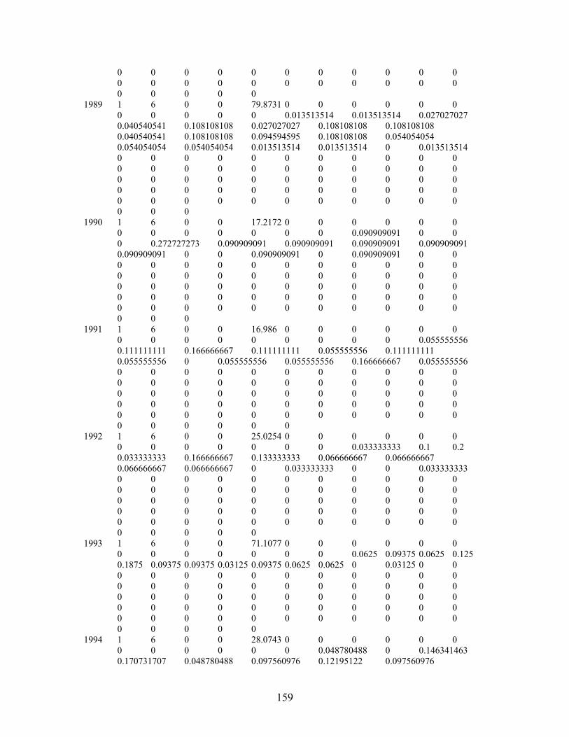
0 0 0 0 0 0 0 0 0 0 0 0 0 0 0 0 0 0 0 0 0 0 0 0 0 0 0 1989 1 6 0 0 79.8731 0 0 0 0 0 0 0 0 0 0 0 0.013513514 0.013513514 0.027027027 0.040540541 0.108108108 0.027027027 0.108108108 0.108108108 0.040540541 0.108108108 0.094594595 0.108108108 0.054054054 0.054054054 0.054054054 0.013513514 0.013513514 0 0.013513514 0 0 0 0 0 0 0 0 0 0 0 0 0 0 0 0 0 0 0 0 0 0 0 0 0 0 0 0 0 0 0 0 0 0 0 0 0 0 0 0 0 0 0 0 0 0 0 0 0 0 0 0 0 0 0 0 0 0 1990 1 6 0 0 17.2172 0 0 0 0 0 0 0 0 0 0 0 0 0 0.090909091 0 0 0 0.272727273 0.090909091 0.090909091 0.090909091 0.090909091 0.090909091 0 0 0.090909091 0 0.090909091 0 0 0 0 0 0 0 0 0 0 0 0 0 0 0 0 0 0 0 0 0 0 0 0 0 0 0 0 0 0 0 0 0 0 0 0 0 0 0 0 0 0 0 0 0 0 0 0 0 0 0 0 0 0 0 0 0 0 0 0 1991 1 6 0 0 16.986 0 0 0 0 0 0 0 0 0 0 0 0 0 0 0 0.055555556 0.111111111 0.166666667 0.111111111 0.055555556 0.111111111 0.055555556 0 0.055555556 0.055555556 0.166666667 0.055555556 0 0 0 0 0 0 0 0 0 0 0 0 0 0 0 0 0 0 0 0 0 0 0 0 0 0 0 0 0 0 0 0 0 0 0 0 0 0 0 0 0 0 0 0 0 0 0 0 0 0 0 0 0 0 0 0 0 0 0 0 0 1992 1 6 0 0 25.0254 0 0 0 0 0 0 0 0 0 0 0 0 0 0.033333333 0.1 0.2 0.033333333 0.166666667 0.133333333 0.066666667 0.066666667 0.066666667 0.066666667 0 0.033333333 0 0 0.033333333 0 0 0 0 0 0 0 0 0 0 0 0 0 0 0 0 0 0 0 0 0 0 0 0 0 0 0 0 0 0 0 0 0 0 0 0 0 0 0 0 0 0 0 0 0 0 0 0 0 0 0 0 0 0 0 0 0 0 0 0 1993 1 6 0 0 71.1077 0 0 0 0 0 0 0 0 0 0 0 0 0 0.0625 0.09375 0.0625 0.125 0.1875 0.09375 0.09375 0.03125 0.09375 0.0625 0.0625 0 0.03125 0 0 0 0 0 0 0 0 0 0 0 0 0 0 0 0 0 0 0 0 0 0 0 0 0 0 0 0 0 0 0 0 0 0 0 0 0 0 0 0 0 0 0 0 0 0 0 0 0 0 0 0 0 0 0 0 0 0 0 0 0 0 1994 1 6 0 0 28.0743 0 0 0 0 0 0 0 0 0 0 0 0 0.048780488 0 0.146341463 0.170731707 0.048780488 0.097560976 0.12195122 0.097560976

159

0.097560976 0.024390244 0 0.048780488 0.048780488 0 0 0.024390244 0 0.024390244 0 0 0 0 0 0 0 0 0 0 0 0 0 0 0 0 0 0 0 0 0 0 0 0 0 0 0 0 0 0 0 0 0 0 0 0 0 0 0 0 0 0 0 0 0 0 0 0 0 0 0 0 0 0 0 0 0 0 1995 1 6 0 0 32.8691 0 0 0 0 0 0 0 0 0 0 0 0.027027027 0.027027027 0.027027027 0.027027027 0.162162162 0.081081081 0.189189189 0.081081081 0.162162162 0.027027027 0.054054054 0.081081081 0 0.027027027 0 0.027027027 0 0 0 0 0 0 0 0 0 0 0 0 0 0 0 0 0 0 0 0 0 0 0 0 0 0 0 0 0 0 0 0 0 0 0 0 0 0 0 0 0 0 0 0 0 0 0 0 0 0 0 0 0 0 0 0 0 0 0 0 0 1996 1 6 0 0 99.7415 0 0 0 0 0 0 0 0 0.009345794 0 0 0.009345794 0.056074766 0.130841121 0.093457944 0.102803738 0.121495327 0.093457944 0.074766355 0.065420561 0.065420561 0.065420561 0.056074766 0.028037383 0 0.009345794 0 0.009345794 0.009345794 0 0 0 0 0 0 0 0 0 0 0 0 0 0 0 0 0 0 0 0 0 0 0 0 0 0 0 0 0 0 0 0 0 0 0 0 0 0 0 0 0 0 0 0 0 0 0 0 0 0 0 0 0 0 0 0 0 0 0 1996 1 6 0 0 20.0009 0 0 0 0 0 0 0 0 0 0 0 0 0.0625 0 0.0625 0 0.0625 0.0625 0.125 0.0625 0.125 0.125 0 0 0.0625 0.125 0 0.0625 0 0 0 0 0.0625 0 0 0 0 0 0 0 0 0 0 0 0 0 0 0 0 0 0 0 0 0 0 0 0 0 0 0 0 0 0 0 0 0 0 0 0 0 0 0 0 0 0 0 0 0 0 0 0 0 0 0 0 0 0 0 1997 1 6 0 0 21.2162 0 0 0 0 0 0 0 0 0 0.016949153 0 0 0 0.016949153 0.084745763 0.271186441 0.101694915 0.152542373 0.101694915 0.016949153 0.152542373 0.016949153 0 0.033898305 0 0.016949153 0 0.016949153 0 0 0 0 0 0 0 0 0 0 0 0 0 0 0 0 0 0 0 0 0 0 0 0 0 0 0 0 0 0 0 0 0 0 0 0 0 0 0 0 0 0 0 0 0 0 0 0 0 0 0 0 0 0 0 0 0 0 0 0 1997 1 6 0 0 17.9703 0 0 0 0 0 0 0 0 0 0.04 0 0 0 0 0.04 0.16 0.08 0.2 0.08 0.04 0.24 0.04 0 0.08 0 0 0 0 0 0 0 0 0 0 0 0 0 0 0 0 0 0 0 0 0 0 0 0 0 0 0 0 0 0 0 0 0 0 0 0 0 0 0 0 0 0 0 0 0 0 0 0 0 0 0 0 0 0 0 0 0 0 0 0 0 0 0 0

160

1998 1 6 0 0 38.7177 0 0 0 0 0 0 0 0 0 0 0.024390244 0 0.024390244 0.024390244 0.073170732 0.170731707 0.146341463 0.195121951 0.048780488 0.12195122 0.097560976 0.048780488 0.024390244 0 0 0 0 0 0 0 0 0 0 0 0 0 0 0 0 0 0 0 0 0 0 0 0 0 0 0 0 0 0 0 0 0 0 0 0 0 0 0 0 0 0 0 0 0 0 0 0 0 0 0 0 0 0 0 0 0 0 0 0 0 0 0 0 0 1998 1 6 0 0 18.5415 0 0 0 0 0 0 0 0 0 0 0.038461538 0 0.038461538 0.038461538 0.076923077 0.192307692 0.269230769 0.153846154 0.038461538 0.115384615 0 0 0 0.038461538 0 0 0 0 0 0 0 0 0 0 0 0 0 0 0 0 0 0 0 0 0 0 0 0 0 0 0 0 0 0 0 0 0 0 0 0 0 0 0 0 0 0 0 0 0 0 0 0 0 0 0 0 0 0 0 0 0 0 0 0 0 0 0 0 2001 1 6 0 0 16.1135 0 0 0 0 0 0 0 0 0 0 0 0 0 0 0.026315789 0.026315789 0.078947368 0.105263158 0.131578947 0.026315789 0.210526316 0.184210526 0.105263158 0.026315789 0.052631579 0.026315789 0 0 0 0 0 0 0 0 0 0 0 0 0 0 0 0 0 0 0 0 0 0 0 0 0 0 0 0 0 0 0 0 0 0 0 0 0 0 0 0 0 0 0 0 0 0 0 0 0 0 0 0 0 0 0 0 0 0 0 0 0 0 2003 1 6 0 0 35.2786 0 0 0 0 0 0 0 0 0 0 0 0 0 0 0 0.017857143 0.107142857 0.071428571 0.107142857 0.142857143 0.178571429 0.053571429 0.089285714 0.089285714 0.035714286 0.035714286 0.017857143 0.017857143 0.017857143 0 0 0 0 0.017857143 0 0 0 0 0 0 0 0 0 0 0 0 0 0 0 0 0 0 0 0 0 0 0 0 0 0 0 0 0 0 0 0 0 0 0 0 0 0 0 0 0 0 0 0 0 0 0 0 0 0 0 0 0 0 2004 1 6 0 0 35.7447 0 0 0 0 0 0 0 0 0 0 0.041666667 0.041666667 0 0 0 0 0.041666667 0.166666667 0.125 0.083333333 0.166666667 0.166666667 0.041666667 0.083333333 0 0 0 0 0 0 0.041666667 0 0 0 0 0 0 0 0 0 0 0 0 0 0 0 0 0 0 0 0 0 0 0 0 0 0 0 0 0 0 0 0 0 0 0 0 0 0 0 0 0 0 0 0 0 0 0 0 0 0 0 0 0 0 0 0 0 1 #_N_age'_bins #_lower_age_of_age'_bins 1

161

0 #_number_of_ageerr_types #_vector_with_stddev_of ageing_precision_for_each_AGE_and_type 0 #_N_age_observations #Year Season Fleet Gender Mkt ageerr Lbin_lo Lbin_hi Nsamp 0 #_N_size-at-age_observations;_values_on_row1;_N_on_row2 #Year Season Fleet Gender Mkt ageerr Nsamp #_environmental_data 1 # N_variables 0 # N_observations #_Year Variable Value

999 #end of file

162

Appendix B-2. SS2 .CTL File for the NCS # stage-2a - new Format 2 #_N_growthmorphs #_assign_sex_to each_morph_(1=female;_2=male) 1 2 1 #_N_Areas_(populations) #_each_fleet/survey_operates_in_just_one_area #_but_different_fleets/surveys_can be assigned_to_share_same_selex(FUTURE_coding) 1 1 1 1 1 1 1 #area_for_each_fleet/survey 0 #do_migration_(0/1) 0 #_N_Block_Designs #0 #_N_Blocks_per_Design(Block_1_always_starts_in_styr) #1975 1985 1986 1990 1995 2001 #_Block_Design_1 #_Block_Design_2 #1987 1990 #1995 2001 #Natural_mortality_and_growth_parameters_for_each_morph 0 #_Last_age_for_natmort_young 0 #_First_age_for_natmort_old 0 #_age_for_growth_Lmin 17 #_age_for_growth_Lmax -4 #_MGparm_dev_phase # LO HI INIT PRIOR PR_type SD PHASE env-variable use_dev dev_minyr dev_maxyr dev_stddev 0.02 0.5 0.25 0.26 0 0.8 -3 0 0 0 0 0.5 0 0 #M1_natM_young 0 0.5 0 0 0 0.8 -3 0 0 0 0 0.5 0 0 #M1_natM_old_as_exponential_offset(rel_young) 1 40 10.79 19.26 0 10 -2 0 0 0 0 0.5 0 0 #M1_Lmin 40 90 59.71 62.13 0 10 -2 0 0 0 0 0.5 0 0 #M1_Lmax 0.05 0.25 0.18 0.185 0 0.8 -3 0 0 0 0 0.5 0 0 #M1_VBK 0.14 0.14 0.14 0.139 0 0.8 -3 0 0 0 0 0.5 0 0 #M1_CV-young -3 3 -0.4418 -0.049 0 0.8 -3 0 0 0 0 0.5 0 0 #M1_CV-old_as_exponential_offset(rel_young) -3 3 0.1823 -0.1 0 0.8 -3 0 0 0 0 0.5 0 0 #M2_natM_young_as_exponential_offset(rel_morph_1) -3 3 0 0 0 0.8 -3 0 0 0 0 0.5 0 0 #M2_natM_old_as_exponential_offset(rel_young) -3 3 0.2076 0.4 0 0.8 -3 0 0 0 0 0.5 0 0 #M2_Lmin_as_exponential_offset ln(16.93/10.79) -3 3 -0.2488 -0.2 0 0.8 -2 0 0 0 0 0.5 0 0 #M2_Lmax_as_exponential_offset ln(46.75/58.65)=ln(M/F) -3 3 0.442 0.4 0 0.8 -3 0 0 0 0 0.5 0 0 #M2_VBK_as_exponential_offset ln(0.28/0.18) -3 3 0 0 0 0.8 -3 0 0 0 0 0.5 0 0 #M2_CV-young_as_exponential_offset(rel_CV-young_for_morph_1) -3 3 -0.4418 -0.049 0 0.8 -3 0 0 0 0 0.5 0 0 #M2_CV-old_as_exponential_offset(rel_CV-young) ln(0.09/0.14)

163

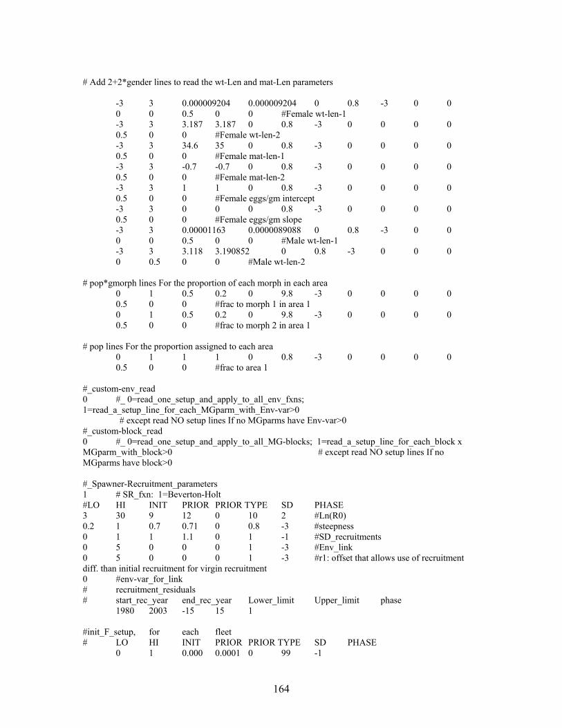
# Add 2+2*gender lines to read the wt-Len and mat-Len parameters -3 3 0.000009204 0.000009204 0 0.8 -3 0 0 0 0 0.5 0 0 #Female wt-len-1 -3 3 3.187 3.187 0 0.8 -3 0 0 0 0 0.5 0 0 #Female wt-len-2 -3 3 34.6 35 0 0.8 -3 0 0 0 0 0.5 0 0 #Female mat-len-1 -3 3 -0.7 -0.7 0 0.8 -3 0 0 0 0 0.5 0 0 #Female mat-len-2 -3 3 1 1 0 0.8 -3 0 0 0 0 0.5 0 0 #Female eggs/gm intercept -3 3 0 0 0 0.8 -3 0 0 0 0 0.5 0 0 #Female eggs/gm slope -3 3 0.00001163 0.0000089088 0 0.8 -3 0 0 0 0 0.5 0 0 #Male wt-len-1 -3 3 3.118 3.190852 0 0.8 -3 0 0 0 0 0.5 0 0 #Male wt-len-2 # pop*gmorph lines For the proportion of each morph in each area 0 1 0.5 0.2 0 9.8 -3 0 0 0 0 0.5 0 0 #frac to morph 1 in area 1 0 1 0.5 0.2 0 9.8 -3 0 0 0 0 0.5 0 0 #frac to morph 2 in area 1 # pop lines For the proportion assigned to each area 0 1 1 1 0 0.8 -3 0 0 0 0 0.5 0 0 #frac to area 1 #_custom-env_read 0 #_ 0=read_one_setup_and_apply_to_all_env_fxns; 1=read_a_setup_line_for_each_MGparm_with_Env-var>0 # except read NO setup lines If no MGparms have Env-var>0 #_custom-block_read 0 #_ 0=read_one_setup_and_apply_to_all_MG-blocks; 1=read_a_setup_line_for_each_block x MGparm_with_block>0 # except read NO setup lines If no MGparms have block>0 #_Spawner-Recruitment_parameters 1 # SR_fxn: 1=Beverton-Holt #LO HI INIT PRIOR PRIOR TYPE SD PHASE 3 30 9 12 0 10 2 #Ln(R0) 0.2 1 0.7 0.71 0 0.8 -3 #steepness 0 1 1 1.1 0 1 -1 #SD_recruitments 0 5 0 0 0 1 -3 #Env_link 0 5 0 0 0 1 -3 #r1: offset that allows use of recruitment diff. than initial recruitment for virgin recruitment 0 #env-var_for_link # recruitment_residuals # start_rec_year end_rec_year Lower_limit Upper_limit phase 1980 2003 -15 15 1 #init_F_setup, for each fleet # LO HI INIT PRIOR PRIOR TYPE SD PHASE 0 1 0.000 0.0001 0 99 -1

164

0 1 0 0.1 0 99 -2 0 1 0 0.1 0 99 -2 0 1 0 0.1 0 99 -2 0 1 0.000 0.0001 0 99 -1 0 1 0.000 0.0001 0 99 -1 #_Qsetup #_add_parm_row_for_each_positive_entry_below(row_then_column) #-Float(0/1) #Do-power(0/1) #Do-env(0/1) #Do-dev(0/1-not implemented) #Env-Var #Biomass(1)/Numbers(2) for each fleet and survey 0 0 0 0 0 1 0 0 0 0 0 1 0 0 0 0 0 1 0 0 0 0 0 1 0 0 0 0 0 1 0 0 0 0 0 1 0 0 0 0 0 2 #LO HI INIT PRIOR PRIOR TYPE SD PHASE #-30 30 0 0.1 20 2 #-30 30 0 0.1 20 2 #-30 30 0 0.1 20 2 #-30 30 0 0.1 20 2 #-30 30 -3 -2 10 1 #log(Q) (if float =1) #-30 30 0.01 -1 1 4 #Q-power #-30 30 0.01 -1 1 4 #Q-env #_SELEX_&_RETENTION_PARAMETERS #Selex_type Do_retention(0/1) Do_male Mirrored_selex_number 1 0 0 0 #_fleet_1 2 0 0 0 #_fleet_2 2 0 0 0 #_fleet_3 2 0 0 0 #_fleet_4 1 0 0 0 #_fleet_5 1 0 0 0 #_fleet_6 5 0 0 6 #_survey_1 #_Age selex 10 0 0 0 #_fleet_1 10 0 0 0 #_fleet_2 10 0 0 0 #_fleet_3 10 0 0 0 #_fleet_4 10 0 0 0 #_fleet_5 10 0 0 0 #_fleet_6 10 0 0 0 #_survey_1 # LO HI INIT PRIOR PR_type SD PHASE env-variable use_dev dev_minyr dev_maxyr dev_stddev Block_Pattern 19 70 45 45 0 10 2 0 0 0 0 0.5 0 0 #infl_for_logistic FLT 1 0.001 30 5 5 0 5 3 0 0 0 0 0.5 0 0 #95%width_for_logistic

165

10 60 40 50 0 10 3 0 0 0 0 0.5 0 0 #peak FLEET 2 LIVE FISH 0.0001 0.1 0.000 0 0 99 -2 0 0 0 0 0.5 0 0 #init -10 5 0.0 0.0 0 3 2 0 0 0 0 0.5 0 0 #infl 0.001 5 0.3 0.3 0 99 3 0 0 0 0 0.5 0 0 #slope -10 10 -5 9 0 99 3 0 0 0 0 0.5 0 0 #final -10 5 0.0 0.0 0 3 4 0 0 0 0 0.5 0 0 #infl2 0.001 50 0.5 .3 0 99 5 0 0 0 0 0.5 0 0 #slope2 0.1 10 1 4 0 99 -5 0 0 0 0 0.5 0 0 #width of top 10 70 30 50 0 10 3 0 0 0 0 0.5 0 0 #peak FLEET 3 Man Made 0.0001 0.1 0.00 0 0 99 -2 0 0 0 0 0.5 0 0 #init -10 5 0.5 0.0 0 3 3 0 0 0 0 0.5 0 0 #infl 0.001 10 0.5 0.3 0 99 -3 0 0 0 0 0.5 0 0 #slope -5 20 -0.5 9 0 99 -3 0 0 0 0 0.5 0 0 #final -10 10 1 0.0 0 3 4 0 0 0 0 0.5 0 0 #infl2 0.001 50 -1 0.3 0 99 5 0 0 0 0 0.5 0 0 #slope2 0.1 50 4 20 0 99 -5 0 0 0 0 0.5 0 0 #width of top 10 70 35 50 0 10 3 0 0 0 0 0.5 0 0 #peak FLEET 4 Shore 0.0001 0.1 0.000 0 0 99 -2 0 0 0 0 0.5 0 0 #init -10 20 0.5 0.0 0 3 3 0 0 0 0 0.5 0 0 #infl 0.001 10 0.5 0.3 0 99 3 0 0 0 0 0.5 0 0 #slope -5 10 0 9 0 99 3 0 0 0 0 0.5 0 0 #final -10 10 1 0.0 0 3 4 0 0 0 0 0.5 0 0 #infl2 0.001 50 -1 0.3 0 99 5 0 0 0 0 0.5 0 0 #slope2 0.1 50 4 20 0 99 -5 0 0 0 0 0.5 0 0 #width of top 19 70 45 45 0 10 2 0 0 0 0 0.5 0 0 #infl_for_logistic FLT 5 PBR 0.001 30 5 5 0 5 3 0 0 0 0 0.5 0 0 #95%width_for_logistic

166

19 70 45 45 0 10 2 0 0 0 0 0.5 0 0 #infl_for_logistic FLT 6 CPFV 0.001 30 5 5 0 5 3 0 0 0 0 0.5 0 0 #95%width_for_logistic 1 44 1 1 0 10 -3 0 0 0 0 0.5 0 0 #min Len bin - fixed SURVEY 1 0.001 100 44 50 0 5 -4 0 0 0 0 0.5 0 0 #max Len bin fixed #_custom-env_read 0 #_custom-block_read 0 -4 #_phase_for_selex_parm_devs 1#Max_lambda_phases:_ 0 #sd_offset #_survey_lambdas 0 0 0 0 0 0 1 #_discard_lambdas 0 0 0 0 0 0 0 #_meanwtlambda(one_for_all_sources) 1 #_lenfreq_lambdas 1 1 0 1 1 1 0 #_age_freq_lambdas 0 0 0 0 0 0 0 #_size@age_lambdas 0 0 0 0 0 0 0 #_initial_equil_catch 0 #_recruitment_lambda 1 #_parm_prior_lambda 1 #_parm_dev_timeseries_lambda 1 # crashpen lambda 100 #max F 0.9 999 #_end-of-file #Q_setup:_add_parm_row_for_each_positive_entry_below(row_then_column)

167

Appendix C-1. SS2 .DAT File for the SCS

#_Number_of_datafiles: 1 #_start_nudata: 1 1916 #_styr 2004 #_endyr 1 #N_seasons_per_year 12 #vector_with_N_months_in_each_season 1 #spawning_season_-_spawning_will_occur_at_beginning_of_this_season 6 #N_fishing_fleets 3 #N_surveys;_data_type_numbers_below_must_be_sequential_with_the_N_fisheries fleet1%fleet2%fleet3%fleet4%fleet5%fleet6%survey1%survey2%survey3 0.5 0.5 0.5 0.5 0.5 0.5 0.5 0.5 0.5#_surveytiming_in_season 2 #number_of_genders(1 / 2) 35 #accumulator_age;_model_always_starts_with_age_0 #Catch (mt) #Fleet 1 #Fleet 2 #Fleet 3 #Fleet 4 #Fleet 5 #Fleet 6 #Comm SoCAL #SoCAL_live #S_Man-made #S_Shore #S_PBR #S_CPFV # Year Season 0 0 0 0 0 0 # initial_equilibrium 0 0 0.022633929 0.020285223 0 0 # 1916 1 0 0 0.022633929 0.020285223 0 0 # 1917 1 0 0 0.022633929 0.020285223 0 0 # 1918 1 0 0 0.022633929 0.020285223 0 0 # 1919 1 0 0 0.022633929 0.020285223 0 0 # 1920 1 0 0 0.022633929 0.020285223 0 0 # 1921 1 0 0 0.022633929 0.020285223 0 0 # 1922 1 0 0 0.022633929 0.020285223 0 0 # 1923 1 0 0 0.022633929 0.020285223 0 0 # 1924 1 0 0 0.022633929 0.020285223 0 0 # 1925 1 0 0 0.022633929 0.020285223 0 0 # 1926 1 0 0 0.022633929 0.020285223 0 0 # 1927 1 0 0 0.022633929 0.020285223 0.0156 0.039 # 1928 1 0 0 0.045267857 0.040570447 0.0312 0.078 # 1929 1 0 0 0.067901786 0.06085567 0.0468 0.117 # 1930 1 0.000453592 0 0.091116071 0.081661028 0.0628 0.157 # 1931 1 0.000907185 0 0.11375 0.101946251 0.0784 0.196 # 1932 1 0.033112239 0 0.136383929 0.122231474 0.094 0.235 # 1933 1 0.000453592 0 0.159017857 0.142516698 0.1096 0.274 # 1934 1 0.067131662 0 0.182232143 0.163322055 0.1256 0.314 # 1935 1 0.006350292 0 0.2559375 0.229379065 0.1764 0.441 # 1936 1 0.001360777 0 0.169464286 0.151879109 0.1168 0.292 # 1937 1 0.000453592 0 0.478794643 0.429110495 0.33 0.825 # 1938 1 0.001360777 0 0.179330357 0.160721385 0.1236 0.309 # 1939 1 0.026761946 0 0.168883929 0.151358975 0.1164 0.291 # 1940 1 0.0353802 0 0.355758929 0.318842101 0.2452 0.613 # 1941 1 0.003628738 0 0.355758929 0.318842101 0.2452 0.613 # 1942 1 0 0 0.355758929 0.318842101 0.2452 0.613 # 1943 1 0.014968546 0 0.355758929 0.318842101 0.2452 0.613 # 1944 1 0 0 0.355758929 0.318842101 0.2452 0.613 # 1945 1 0 0 0.355758929 0.318842101 0.2452 0.613 # 1946 1 0.006350292 0 1.093973214 0.980452465 0.754 1.885 # 1947 1 0.0058967 0 1.231517857 1.103724207 0.8488 2.122 # 1948 1 0.004989515 0 1.603526786 1.437130058 1.1052 2.763 # 1949 1

168

0.289391894 0 1.249508929 1.119848359 0.8612 2.153 # 1950 1 0.019050877 0 1.146785714 1.027784653 0.7904 1.976 # 1951 1 0.050802339 0 1.543169643 1.383036129 1.0636 2.659 # 1952 1 0.014514954 0 2.294732143 2.056609573 1.5816 3.954 # 1953 1 0.001360777 0 5.244107143 4.699930223 3.6144 9.036 # 1954 1 0.008618254 0 5.056651786 4.531926962 3.4852 8.713 # 1955 1 0.057606223 0 5.735089286 5.139963531 8.050630791 9.882 #1956 1 0.36332744 0 4.190178571 3.755367 5.88196259 7.22 #1957 1 0.06667807 0 2.825178571 2.532011988 3.965844029 4.868 #1958 1 0.006803885 0 0.723125 0.648086881 1.015086619 1.246 #1959 1 0.002721554 0 0.346473214 0.310519958 0.486361727 0.597 #1960 1 0.009979031 0 0.409732143 0.367214557 0.575161439 0.706 #1961 1 0.002267962 0 1.259955357 1.12921077 1.768662158 2.171 #1962 1 0.004535923 0 2.535 2.271945021 3.558505899 4.368 # 1963 1 0.069853216 0 2.016741071 1.807465419 2.831 3.475 # 1964 1 0.016329323 0 2.090446429 1.873522428 7.204 3.602 # 1965 1 0.050802339 0 3.196026786 2.864377572 11.014 5.507 # 1966 1 0.037648162 0 1.6534375 2.42165 5.698 2.849 # 1967 1 0.06078137 0 1.177544643 1.72465 4.058 2.029 # 1968 1 0.042637677 0 1.1253125 1.64815 3.878 1.939 # 1969 1 0.09026487 0 1.435223214 2.10205 4.946 2.473 # 1970 1 0.0235868 0 1.484553571 2.1743 10.232 2.558 # 1971 1 0.037194569 0 4.328883929 6.34015 29.836 7.459 # 1972 1 0.014514954 0 1.732946429 2.5381 11.944 2.986 # 1973 1 0.0648637 0 1.766607143 2.5874 12.176 3.044 # 1974 1 0.027215539 0 2.623794643 3.84285 18.084 4.521 # 1975 1 0.089357685 0 1.738169643 2.54575 11.98 2.995 # 1976 1 0.107047785 0 1.123571429 1.6456 7.744 1.936 # 1977 1 0.319782578 0 1.658660714 2.4293 11.432 2.858 # 1978 1 0.21409557 0 1.240803571 1.8173 8.552 2.138 # 1979 1 3.572039439 0 2.287276949 24.28264818 156.824185 3.043394524 #1980 1 0.259908393 0 0.308513612 9.316412523 25.51136875 3.465066157 #1981 1 0.152860608 0 0.399851606 4.122956505 48.48580236 2.061955856 #1982 1 0.185972847 0 1.004152196 3.381780524 12.73756525 1.739988905 #1983 1 0.0530703 0 1.433987883 10.01679734 27.35597033 0.631265372 #1984 1 0.114758854 0 0.813499478 5.594826462 25.78336369 0.456260341 #1985 1 0.18461207 0 1.026352 3.7219205 30.75871882 1.697173958 #1986 1 0.290299078 0 1.014208 3.677882 25.98283703 3.477591651 #1987 1 0.493054841 0 1.08376 3.9301025 11.98452193 1.40365712 #1988 1 0.458128233 0 1.46464 5.31131 7.834712066 2.321754077 #1989 1 0.605999326 0 1.749472 6.344213 29.04694 4.42122 #1990 1 1.596191338 0 1.63024 5.911835 27.0673 4.1199 #1991 1 0.461303379 0 0.943552 3.421658 15.66604 2.38452 #1992 1 0.387367833 0.004082331 0.068191985 0.372852753 3.615335 1.49455#1993 1 0.703521672 5.482116656 0.381984 0.716557479 10.58852564 1.193553213#1994 1 0.78743625 9.655165905 0.672649083 1.313871787 1.751247422 0.838858431 0.454953087 10.47027129 1.336033481 0.264610598 8.609793004 2.723841859 0.630493311 11.71946451 0.949072 0.629774821 2.939099936 1.620110787 0.66768788 16.57018067 0.65136 1.818910405 4.72988573 3.185354609 0.320236171 14.00647693 0.818339996 2.189281708 11.59394183 1.040713461 0.850939173 21.44130848 0.140301836 0.435422308 5.506288144 1.818307695 0.605545734 13.51024695 1.013583537 2.399197116 3.464955588 1.093646118 0.35743074 6.359817775 0.173477764 3.454976208 5.723285614 1.823330904 0.360605886 5.406820332 0.506464518 1.859074105 6.364332926 1.317286472 0.167375562 4.083691565 0.390548387 3.592009512 2.295529853 2.265961028

169

#Abundance_Indices 96 #_N_observations #Year Season Type Value CV 1960 1 7 0.0004068 0.73521986 #soCAL 1961 1 7 0.000752368 2.149104207 1962 1 7 0.001638443 0.395887617 1963 1 7 0.002358607 0.706942173 1964 1 7 0.002327071 0.254499182 1965 1 7 0.001863092 0.197943809 1966 1 7 0.002484396 1.131107477 1967 1 7 0.00176781 0.311054556 1968 1 7 0.001068786 0.791775234 1969 1 7 0.001125285 0.73521986 1970 1 7 0.001109469 0.480720678 1971 1 7 0.001348063 0.537276052 1972 1 7 0.002392308 1.272495912 1973 1 7 0.001179491 0.508998365 1974 1 7 0.001610348 0.339332243 1975 1 7 0.002238103 0.339332243 1976 1 7 0.001736429 0.311054556 1977 1 7 0.001145585 0.226221495 1978 1 7 0.001462472 0.311054556 1980 1 7 0.001237435 0.36760993 1981 1 7 0.001234042 0.282776869 1982 1 7 0.000856295 0.311054556 1983 1 7 0.000796743 0.311054556 1984 1 7 0.000232116 0.537276052 1985 1 7 0.000468776 1.979438085 1986 1 7 0.001336265 0.282776869 1987 1 7 0.00168358 0.254499182 1988 1 7 0.001447898 0.311054556 1989 1 7 0.002488253 0.254499182 1990 1 7 0.00303796 0.254499182 1991 1 7 0.002070488 0.254499182 1992 1 7 0.001206023 0.197943809 1993 1 7 0.000736278 0.36760993 1994 1 7 0.000450407 3.478155493 1995 1 7 0.000632539 0.452442991 1996 1 7 0.001158318 0.508998365 1997 1 7 0.000840106 0.424165304 1998 1 7 0.000342289 0.424165304 1999 1 7 0.000341477 0.537276052 2000 1 7 0.000642221 1.922882711 2001 1 7 0.00083581 0.36760993 2002 1 7 0.000440773 0.791775234 2003 1 7 0.000381094 0.480720678 1978 1 8 63.18 2.035633936 #CalCOFI:manta 1980 1 8 100.16 1.395863271 1981 1 8 43.57 0.872414544 1984 1 8 39.44 0.814253575 1985 1 8 74.52 0.901495029 1986 1 8 29.46 0.988736483 1987 1 8 32.96 1.337702301 1988 1 8 31.43 0.872414544 1989 1 8 87.16 0.610690181

170

1990 1 8 44.32 1.45402424 1991 1 8 85.75 0.930575514 1992 1 8 16.66 1.948392482 1993 1 8 16.82 1.45402424 1994 1 8 16.66 1.686668119 1995 1 8 30.34 1.105058423 1996 1 8 33.24 1.017816968 1997 1 8 46.69 1.075977938 1998 1 8 3.16 0.843334059 1999 1 8 52.95 0.843334059 2000 1 8 40.23 1.046897453 2001 1 8 29.37 1.075977938 2002 1 8 112.91 0.988736483 1972 1 9 13.57 0.78128954 #Impingement 1973 1 9 17.22 0.710263218 1974 1 9 6.52 0.639236896 1975 1 9 9.38 0.532697413 1976 1 9 7.12 0.568210574 1977 1 9 4.39 0.816802701 1978 1 9 3.31 0.745776379 1979 1 9 1.48 0.78128954 1980 1 9 1.7 0.710263218 1981 1 9 2.76 0.852315861 1982 1 9 2.3 0.923342183 1983 1 9 2.36 0.852315861 1984 1 9 2.46 0.78128954 1985 1 9 2.36 0.745776379 1986 1 9 1.58 0.852315861 1987 1 9 2.65 0.710263218 1988 1 9 1.04 1.20744747 1989 1 9 2.59 0.852315861 1990 1 9 1.73 0.923342183 1991 1 9 2.39 0.816802701 1992 1 9 1.51 0.852315861 1993 1 9 0.56 1.20744747 1994 1 9 0.8 1.278473792 1995 1 9 0.84 1.562579079 1996 1 9 0.76 1.527065918 1997 1 9 1.32 1.385013275 1998 1 9 0.77 1.456039597 1999 1 9 5.87 0.78128954 2000 1 9 4.26 1.136421149 2001 1 9 6.02 1.740144884 2002 1 9 8.27 1.029881666 #_Discard_Biomass 1 #_(1=biomass;_2=fraction) 0 #_N_observations #Year Season Type Value CV #_Mean_BodyWt 66 #16 #Year Seas Type Mkt Value CV 1980 1 3 0 0.492279553 0.516130363 1981 1 3 0 0.419000775 0.645246975

171

1982 1 3 0 0.493063014 0.285650358 1983 1 3 0 0.582606394 0.66005437 1984 1 3 0 0.447899911 0.562729878 1985 1 3 0 0.262511582 0.49685921 1987 1 3 0 0.813149287 0.542383153 1989 1 3 0 0.844692038 0.820356296 1999 1 3 0 0.31451741 0.701299103 2000 1 3 0 0.049254253 0.386734508 1980 1 4 0 1.133678516 0.537232412 1981 1 4 0 0.77994266 0.505115433 1982 1 4 0 0.805991794 0.517202794 1983 1 4 0 0.738672454 0.561826014 1984 1 4 0 0.886476707 0.224471437 1985 1 4 0 0.797895245 0.493145332 1986 1 4 0 0.88600727 0.756979078 1987 1 4 0 1.060353528 0.54552634 1988 1 4 0 1.126576808 0.534704585 1989 1 4 0 1.364180271 0.531733214 1995 1 4 0 0.362203113 0.547912403 1996 1 4 0 0.556445073 0.254711646 1998 1 4 0 0.783191181 0.517260685 1999 1 4 0 0.755204318 0.317734566 2002 1 4 0 1.592516625 0.532034869 2003 1 4 0 0.692474995 0.145785004 2004 1 4 0 0.674016928 0.045379857 1980 1 5 0 1.291815069 0.492771083 1981 1 5 0 1.256246743 0.507110937 1982 1 5 0 1.058760669 0.567428189 1983 1 5 0 0.820683443 0.526648444 1984 1 5 0 1.038178219 0.431150315 1985 1 5 0 1.138877816 0.716713535 1986 1 5 0 0.84469507 0.655202169 1987 1 5 0 1.067968135 0.646030012 1988 1 5 0 0.777949064 0.36920555 1989 1 5 0 1.101149157 0.555970093 1993 1 5 0 0.471922251 0.230985364 1994 1 5 0 1.197234596 0.688265236 1995 1 5 0 0.666247912 0.281595989 1996 1 5 0 0.682121989 0.348046861 1997 1 5 0 1.416831368 0.517812268 1998 1 5 0 0.756209444 0.108261896 1999 1 5 0 0.678771359 0.455564135 2000 1 5 0 1.661831759 0.51780411 2001 1 5 0 0.677864698 0.164581821 2002 1 5 0 0.790203587 0.629333135 2003 1 5 0 0.975778341 0.419300425 2004 1 5 0 1.201594209 0.570482102 1980 1 6 0 0.96903267 0.586526236 1981 1 6 0 1.024516638 0.495414495 1982 1 6 0 0.751158095 0.802613803 1983 1 6 0 0.789939908 0.630483077 1984 1 6 0 1.039984011 0.464684213 1985 1 6 0 0.557513617 0.496718316 1986 1 6 0 0.594435488 0.342576808 1987 1 6 0 1.160390128 0.426335328 1988 1 6 0 0.510470251 0.560136709

172

1989 1 6 0 0.694230707 0.649223058 1994 1 6 0 0.94064579 0.221898574 1996 1 6 0 0.653026338 0.150768289 1998 1 6 0 1.012405152 0.667733344 1999 1 6 0 0.462834641 0.271836437 2000 1 6 0 0.706180788 0.211111379 2003 1 6 0 2.174173135 0.378784743 2004 1 6 0 1.615799715 0.445630383 0.0001 #min_proportion_for_compressing_tails_of_observed_composition 0.0001 #_constant added to expected frequencies 44 #_N_length_bins #_lower_edge_of_length_bins 6 8 10 12 14 16 18 20 22 24 26 28 30 32 34 36 38 40 42 44 46 48 50 52 54 56 58 60 62 64 66 68 70 72 74 76 78 80 82 84 86 88 90 92 15 #N_observations #Year Seas Fleet sexes Mkt Nsamp begin data: females then males 1994 1 5 0 0 16.9004 0 0 0 0 0 0 0 0 0 0 0 0 0.066666667 0.133333333 0.2 0.066666667 0.066666667 0.066666667 0 0.066666667 0 0.066666667 0 0 0.066666667 0.066666667 0 0.133333333 0 0 0 0 0 0 0 0 0 0 0 0 0 0 0 0 0 0 0 0 0 0 0 0 0 0 0 0 0 0 0 0 0 0 0 0 0 0 0 0 0 0 0 0 0 0 0 0 0 0 0 0 0 0 0 0 0 0 0 0 1996 1 5 0 0 42.3879 0 0 0 0 0 0 0 0 0 0.034482759 0.034482759 0.137931034 0.206896552 0.206896552 0.137931034 0.034482759 0.137931034 0 0.034482759 0 0 0 0 0 0 0 0 0 0.034482759 0 0 0 0 0 0 0 0 0 0 0 0 0 0 0 0 0 0 0 0 0 0 0 0 0 0 0 0 0 0 0 0 0 0 0 0 0 0 0 0 0 0 0 0 0 0 0 0 0 0 0 0 0 0 0 0 0 0 0 1998 1 5 0 0 11.7108 0 0 0 0 0 0 0 0 0 0 0.095238095 0.047619048 0 0.285714286 0.285714286 0.142857143 0 0.095238095 0.047619048 0 0 0 0 0 0 0 0 0 0 0 0 0 0 0 0 0 0 0 0 0 0 0 0 0 0 0 0 0 0 0 0 0 0 0 0 0 0 0 0 0 0 0 0 0 0 0 0 0 0 0 0 0 0 0 0 0 0 0 0 0 0 0 0 0 0 0 0 0 1999 1 5 0 0 40.3432 0 0 0 0 0 0 0.025 0 0.025 0.025 0 0.075 0.025 0.125 0.25 0.175 0.125 0.05 0.05 0.025 0 0 0 0.025 0 0 0 0 0 0 0 0 0 0 0 0 0 0 0

173

0 0 0 0 0 0 0 0 0 0 0 0 0 0 0 0 0 0 0 0 0 0 0 0 0 0 0 0 0 0 0 0 0 0 0 0 0 0 0 0 0 0 0 0 0 0 0 0 0 2002 1 5 0 0 16.904 0 0 0 0 0 0 0 0 0 0 0 0 0.272727273 0.227272727 0.227272727 0.045454545 0.045454545 0 0.045454545 0.090909091 0 0 0 0.045454545 0 0 0 0 0 0 0 0 0 0 0 0 0 0 0 0 0 0 0 0 0 0 0 0 0 0 0 0 0 0 0 0 0 0 0 0 0 0 0 0 0 0 0 0 0 0 0 0 0 0 0 0 0 0 0 0 0 0 0 0 0 0 0 0 2003 1 5 0 0 44.6519 0 0 0 0 0 0 0 0 0 0 0 0.034482759 0.034482759 0.172413793 0.206896552 0.172413793 0.103448276 0.137931034 0 0.034482759 0.034482759 0 0.034482759 0.034482759 0 0 0 0 0 0 0 0 0 0 0 0 0 0 0 0 0 0 0 0 0 0 0 0 0 0 0 0 0 0 0 0 0 0 0 0 0 0 0 0 0 0 0 0 0 0 0 0 0 0 0 0 0 0 0 0 0 0 0 0 0 0 0 0 2004 1 5 0 0 42.2045 0 0 0 0 0 0 0 0 0 0.00862069 0 0.017241379 0.060344828 0.077586207 0.112068966 0.086206897 0.103448276 0.163793103 0.086206897 0.077586207 0.060344828 0.043103448 0.034482759 0.025862069 0.025862069 0 0.00862069 0 0 0 0 0.00862069 0 0 0 0 0 0 0 0 0 0 0 0 0 0 0 0 0 0 0 0 0 0 0 0 0 0 0 0 0 0 0 0 0 0 0 0 0 0 0 0 0 0 0 0 0 0 0 0 0 0 0 0 0 0 0 0 1975 1 6 0 0 65.9217 0 0 0 0 0 0 0.013157895 0 0.013157895 0.026315789 0.092105263 0.078947368 0.144736842 0.171052632 0.078947368 0.118421053 0.039473684 0.078947368 0.039473684 0.026315789 0.026315789 0.026315789 0 0.013157895 0 0 0.013157895 0 0 0 0 0 0 0 0 0 0 0 0 0 0 0 0 0 0 0 0 0 0 0 0 0 0 0 0 0 0 0 0 0 0 0 0 0 0 0 0 0 0 0 0 0 0 0 0 0 0 0 0 0 0 0 0 0 0 0 0 0 1976 1 6 0 0 82.878 0 0 0 0.010526316 0 0 0 0.010526316 0.010526316 0.052631579 0.063157895 0.105263158 0.189473684 0.094736842 0.063157895 0.084210526 0.052631579 0.084210526 0.031578947 0.042105263 0.021052632 0.021052632 0.042105263 0 0.010526316 0.010526316 0 0 0 0 0 0 0 0 0 0 0 0 0 0 0 0 0 0 0 0 0 0 0 0 0 0 0 0 0 0 0 0 0 0 0 0 0 0 0 0 0 0 0 0 0 0

174

0 0 0 0 0 0 0 0 0 0 0 0 0 0 0 0 1977 1 6 0 0 82.9085 0 0 0 0 0.013157895 0 0 0 0 0.065789474 0.118421053 0.131578947 0.144736842 0.065789474 0.092105263 0.092105263 0.052631579 0.039473684 0.052631579 0.013157895 0.039473684 0.039473684 0 0.013157895 0.013157895 0 0 0 0.013157895 0 0 0 0 0 0 0 0 0 0 0 0 0 0 0 0 0 0 0 0 0 0 0 0 0 0 0 0 0 0 0 0 0 0 0 0 0 0 0 0 0 0 0 0 0 0 0 0 0 0 0 0 0 0 0 0 0 0 0 1978 1 6 0 0 141.586 0 0 0 0.00990099 0 0 0.01980198 0.00990099 0 0.04950495 0.04950495 0.069306931 0.118811881 0.079207921 0.108910891 0.079207921 0.04950495 0.089108911 0.079207921 0.02970297 0.02970297 0.03960396 0 0.03960396 0.03960396 0 0.00990099 0 0 0 0 0 0 0 0 0 0 0 0 0 0 0 0 0 0 0 0 0 0 0 0 0 0 0 0 0 0 0 0 0 0 0 0 0 0 0 0 0 0 0 0 0 0 0 0 0 0 0 0 0 0 0 0 0 0 0 0 0 1986 1 6 0 0 123.608 0 0 0 0 0 0 0.012195122 0.012195122 0.073170732 0.182926829 0.158536585 0.195121951 0.170731707 0.048780488 0.036585366 0.036585366 0.036585366 0 0.024390244 0.012195122 0 0 0 0 0 0 0 0 0 0 0 0 0 0 0 0 0 0 0 0 0 0 0 0 0 0 0 0 0 0 0 0 0 0 0 0 0 0 0 0 0 0 0 0 0 0 0 0 0 0 0 0 0 0 0 0 0 0 0 0 0 0 0 0 0 0 0 0 1987 1 6 0 0 68.4037 0 0 0 0 0 0 0 0 0.02 0.01 0.13 0.12 0.25 0.13 0.12 0.09 0.09 0.03 0.01 0 0 0 0 0 0 0 0 0 0 0 0 0 0 0 0 0 0 0 0 0 0 0 0 0 0 0 0 0 0 0 0 0 0 0 0 0 0 0 0 0 0 0 0 0 0 0 0 0 0 0 0 0 0 0 0 0 0 0 0 0 0 0 0 0 0 0 0 0 1988 1 6 0 0 62.8068 0 0 0 0 0 0 0 0 0.015384615 0.061538462 0.046153846 0.076923077 0.123076923 0.153846154 0.123076923 0.092307692 0.107692308 0.153846154 0.015384615 0.015384615 0 0 0.015384615 0 0 0 0 0 0 0 0 0 0 0 0 0 0 0 0 0 0 0 0 0 0 0 0 0 0 0 0 0 0 0 0 0 0 0 0 0 0 0 0 0 0 0 0 0 0 0 0 0 0 0 0 0 0 0 0 0 0 0 0 0 0 0 0 0 1989 1 6 0 0 81.3786 0 0 0 0 0 0.010752688 0 0.021505376 0.064516129 0.161290323 0.161290323 0.086021505 0.096774194 0.086021505 0.064516129 0.086021505

175

0.032258065 0.010752688 0.032258065 0.010752688 0.010752688 0.043010753 0.021505376 0 0 0 0 0 0 0 0 0 0 0 0 0 0 0 0 0 0 0 0 0 0 0 0 0 0 0 0 0 0 0 0 0 0 0 0 0 0 0 0 0 0 0 0 0 0 0 0 0 0 0 0 0 0 0 0 0 0 0 0 0 0 0 0 0 #1975 1 9 0 0 24.3005 0.04 0 0.02 0 0 0.08 0.12 0.26 0.16 0.2 0.06 0.04 0.02 0 0 0 0 0 0 0 0 0 0 0 0 0 0 0 0 0 0 0 0 0 0 0 0 0 0 0 0 0 0 0 0 0 0 0 0 0 0 0 0 0 0 0 0 0 0 0 0 0 0 0 0 0 0 0 0 0 0 0 0 0 0 0 0 0 0 0 0 0 0 0 0 0 0 0 #1976 1 9 0 0 12.993 0 0 0 0.036036036 0.072072072 0.063063063 0.135135135 0.153153153 0.216216216 0.09009009 0.09009009 0.099099099 0.027027027 0.009009009 0.009009009 0 0 0 0 0 0 0 0 0 0 0 0 0 0 0 0 0 0 0 0 0 0 0 0 0 0 0 0 0 0 0 0 0 0 0 0 0 0 0 0 0 0 0 0 0 0 0 0 0 0 0 0 0 0 0 0 0 0 0 0 0 0 0 0 0 0 0 0 0 0 0 0 0 #1977 1 9 0 0 41.3601 0.016949153 0 0.050847458 0.016949153 0.016949153 0.033898305 0.06779661 0.084745763 0.13559322 0.101694915 0.152542373 0.152542373 0.101694915 0.033898305 0.016949153 0 0 0.016949153 0 0 0 0 0 0 0 0 0 0 0 0 0 0 0 0 0 0 0 0 0 0 0 0 0 0 0 0 0 0 0 0 0 0 0 0 0 0 0 0 0 0 0 0 0 0 0 0 0 0 0 0 0 0 0 0 0 0 0 0 0 0 0 0 0 0 0 0 0 0 #1978 1 9 0 0 0.576864 0 0 0 0 0 0 0 0.142857143 0.238095238 0.285714286 0.095238095 0.142857143 0.095238095 0 0 0 0 0 0 0 0 0 0 0 0 0 0 0 0 0 0 0 0 0 0 0 0 0 0 0 0 0 0 0 0 0 0 0 0 0 0 0 0 0 0 0 0 0 0 0 0 0 0 0 0 0 0 0 0 0 0 0 0 0 0 0 0 0 0 0 0 0 0 0 0 0 0 0 #1992 1 9 0 0 36.2166 0.041666667 0 0.020833333 0 0.020833333 0.083333333 0.104166667 0.0625 0.145833333 0.208333333 0.083333333 0.041666667 0.041666667 0.020833333 0.020833333 0.020833333 0 0 0.0625 0.020833333 0 0 0 0 0 0 0 0 0 0 0 0 0 0 0 0 0 0 0 0 0 0 0 0 0 0 0 0 0 0 0 0 0 0 0 0 0 0 0 0 0 0 0 0 0 0 0 0

176

0 0 0 0 0 0 0 0 0 0 0 0 0 0 0 0 0 0 0 0 #1993 1 9 0 0 10.6635 0.125 0 0.03125 0.0625 0.03125 0 0.03125 0.125 0.125 0.15625 0 0 0.15625 0.0625 0 0 0.03125 0 0.03125 0 0.03125 0 0 0 0 0 0 0 0 0 0 0 0 0 0 0 0 0 0 0 0 0 0 0 0 0 0 0 0 0 0 0 0 0 0 0 0 0 0 0 0 0 0 0 0 0 0 0 0 0 0 0 0 0 0 0 0 0 0 0 0 0 0 0 0 0 0 0 #1994 1 9 0 0 8.63632 0.096774194 0.032258065 0.129032258 0.064516129 0 0.032258065 0.096774194 0.064516129 0.129032258 0.064516129 0.032258065 0.096774194 0.032258065 0.032258065 0 0.032258065 0 0.032258065 0 0 0.032258065 0 0 0 0 0 0 0 0 0 0 0 0 0 0 0 0 0 0 0 0 0 0 0 0 0 0 0 0 0 0 0 0 0 0 0 0 0 0 0 0 0 0 0 0 0 0 0 0 0 0 0 0 0 0 0 0 0 0 0 0 0 0 0 0 0 0 0 #1995 1 9 0 0 4.65097 0.117647059 0.235294118 0.235294118 0 0 0.058823529 0.117647059 0 0 0.058823529 0.117647059 0 0.058823529 0 0 0 0 0 0 0 0 0 0 0 0 0 0 0 0 0 0 0 0 0 0 0 0 0 0 0 0 0 0 0 0 0 0 0 0 0 0 0 0 0 0 0 0 0 0 0 0 0 0 0 0 0 0 0 0 0 0 0 0 0 0 0 0 0 0 0 0 0 0 0 0 0 0 0 #1996 1 9 0 0 6.84423 0.136363636 0.045454545 0 0 0 0 0.045454545 0.181818182 0.181818182 0.136363636 0.181818182 0.045454545 0.045454545 0 0 0 0 0 0 0 0 0 0 0 0 0 0 0 0 0 0 0 0 0 0 0 0 0 0 0 0 0 0 0 0 0 0 0 0 0 0 0 0 0 0 0 0 0 0 0 0 0 0 0 0 0 0 0 0 0 0 0 0 0 0 0 0 0 0 0 0 0 0 0 0 0 0 0 #1997 1 9 0 0 23.9716 0.08 0.04 0 0 0.04 0 0.04 0.08 0.16 0.2 0.04 0.12 0.04 0 0 0.04 0.04 0.04 0 0 0.04 0 0 0 0 0 0 0 0 0 0 0 0 0 0 0 0 0 0 0 0 0 0 0 0 0 0 0 0 0 0 0 0 0 0 0 0 0 0 0 0 0 0 0 0 0 0 0 0 0 0 0 0 0 0 0 0 0 0 0 0 0 0 0 0 0 0 0 #1998 1 9 0 0 3.1703 0.44 0.16 0.04 0 0 0 0.04 0 0.04 0.12 0.04 0.04 0.04 0 0 0 0.04 0 0 0 0 0 0 0 0 0 0 0 0 0 0 0 0 0 0 0 0 0 0 0 0 0 0 0 0 0 0 0 0 0 0 0 0 0 0 0 0 0 0 0 0

177

0 0 0 0 0 0 0 0 0 0 0 0 0 0 0 0 0 0 0 0 0 0 0 0 0 0 0 #1999 1 9 0 0 1.59954 0.615635179 0.218241042 0.068403909 0.03257329 0.013029316 0.022801303 0.006514658 0.009771987 0.003257329 0.003257329 0 0 0.003257329 0 0.003257329 0 0 0 0 0 0 0 0 0 0 0 0 0 0 0 0 0 0 0 0 0 0 0 0 0 0 0 0 0 0 0 0 0 0 0 0 0 0 0 0 0 0 0 0 0 0 0 0 0 0 0 0 0 0 0 0 0 0 0 0 0 0 0 0 0 0 0 0 0 0 0 0 0 #2000 1 9 0 0 2.90412 0.375 0.291666667 0.041666667 0.016666667 0.025 0.075 0.05 0.033333333 0.033333333 0.016666667 0.008333333 0.008333333 0.025 0 0 0 0 0 0 0 0 0 0 0 0 0 0 0 0 0 0 0 0 0 0 0 0 0 0 0 0 0 0 0 0 0 0 0 0 0 0 0 0 0 0 0 0 0 0 0 0 0 0 0 0 0 0 0 0 0 0 0 0 0 0 0 0 0 0 0 0 0 0 0 0 0 0 0 #2001 1 9 0 0 0.536391 0.25 0.472222222 0.111111111 0.083333333 0 0 0 0.027777778 0.055555556 0 0 0 0 0 0 0 0 0 0 0 0 0 0 0 0 0 0 0 0 0 0 0 0 0 0 0 0 0 0 0 0 0 0 0 0 0 0 0 0 0 0 0 0 0 0 0 0 0 0 0 0 0 0 0 0 0 0 0 0 0 0 0 0 0 0 0 0 0 0 0 0 0 0 0 0 0 0 0 #2002 1 9 0 0 1.65306 0.564935065 0.279220779 0.084415584 0.025974026 0.019480519 0.006493506 0 0 0 0.019480519 0 0 0 0 0 0 0 0 0 0 0 0 0 0 0 0 0 0 0 0 0 0 0 0 0 0 0 0 0 0 0 0 0 0 0 0 0 0 0 0 0 0 0 0 0 0 0 0 0 0 0 0 0 0 0 0 0 0 0 0 0 0 0 0 0 0 0 0 0 0 0 0 0 0 0 0 0 0 1 #_N_age'_bins 1 #_lower_age_of_age'_bins 0 #_number_of_ageerr_types #_vector_with_stddev_of ageing_precision_for_each_AGE_and_type 0 #_N_age_observations #Year Season Fleet Gender Mkt ageerr Lbin_lo Lbin_hi Nsamp 0 #_N_size-at-age_observations;_values_on_row1;_N_on_row2 #Year Season Fleet Gender Mkt ageerr Nsamp #_environmental_data 1 # N_variables 0 # N_observations 999 #end of file

178

Appendix C-2. SS2 .CTL File for the SCS # stage-2a - new Format 2 #_N_growthmorphs #_assign_sex_to each_morph_(1=female;_2=male) 1 2 1 #_N_Areas_(populations) #_each_fleet/survey_operates_in_just_one_area #_but_different_fleets/surveys_can be assigned_to_share_same_selex(FUTURE_coding) 1 1 1 1 1 1 1 1 1 #area_for_each_fleet/survey 0 #do_migration_(0/1) 0 #_N_Block_Designs #0 #_N_Blocks_per_Design(Block_1_always_starts_in_styr) #1975 1985 1986 1990 1995 2001 #_Block_Design_1 #_Block_Design_2 #1987 1990 #1995 2001 #Natural_mortality_and_growth_parameters_for_each_morph 0 #_Last_age_for_natmort_young 0 #_First_age_for_natmort_old 0 #_age_for_growth_Lmin 17 #_age_for_growth_Lmax -4 #_MGparm_dev_phase # LO HI INIT PRIOR PR_type SD PHASE env-variable use_dev dev_minyr dev_maxyr dev_stddev 0.02 0.5 0.25 0.26 0 0.8 -3 0 0 0 0 0.5 0 0 #M1_natM_young 0 0.5 0 0 0 0.8 -3 0 0 0 0 0.5 0 0 #M1_natM_old_as_exponential_offset(rel_young) 1 40 10.79 19.26 0 10 -2 0 0 0 0 0.5 0 0 #M1_Lmin 40 90 59.71 62.13 0 10 -2 0 0 0 0 0.5 0 0 #M1_Lmax 0.05 0.25 0.18 0.185 0 0.8 -3 0 0 0 0 0.5 0 0 #M1_VBK 0.14 0.14 0.14 0.139 0 0.8 -3 0 0 0 0 0.5 0 0 #M1_CV-young -3 3 -0.4418 -0.049 0 0.8 -3 0 0 0 0 0.5 0 0 #M1_CV-old_as_exponential_offset(rel_young) -3 3 0.1823 -0.1 0 0.8 -3 0 0 0 0 0.5 0 0 #M2_natM_young_as_exponential_offset(rel_morph_1) -3 3 0 0 0 0.8 -3 0 0 0 0 0.5 0 0 #M2_natM_old_as_exponential_offset(rel_young) -3 3 0.2076 0.4 0 0.8 -3 0 0 0 0 0.5 0 0 #M2_Lmin_as_exponential_offset ln(13.28/10.79) -3 3 -0.2488 -0.2 0 0.8 -2 0 0 0 0 0.5 0 0 #M2_Lmax_as_exponential_offset ln(46.72/60.72)=ln(M/F) -3 3 0.442 0.4 0 0.8 -3 0 0 0 0 0.5 0 0 #M2_VBK_as_exponential_offset ln(0.28/0.18) -3 3 0 0 0 0.8 -3 0 0 0 0 0.5 0 0 #M2_CV-young_as_exponential_offset(rel_CV-young_for_morph_1) -3 3 -0.4418 -0.049 0 0.8 -3 0 0 0 0 0.5 0 0 #M2_CV-old_as_exponential_offset(rel_CV-young) ln(0.09/0.14)

179

# Add 2+2*gender lines to read the wt-Len and mat-Len parameters -3 3 0.00001236 0.0000089088 0 0.8 -3 0 0 0 0 0.5 0 0 #Female wt-len-1 -3 3 3.113 3.190852 0 0.8 -3 0 0 0 0 0.5 0 0 #Female wt-len-2 -3 3 34.6 35 0 0.8 -3 0 0 0 0 0.5 0 0 #Female mat-len-1 -3 3 -0.7 -0.7 0 0.8 -3 0 0 0 0 0.5 0 0 #Female mat-len-2 -3 3 1 1 0 0.8 -3 0 0 0 0 0.5 0 0 #Female eggs/gm intercept -3 3 0 0 0 0.8 -3 0 0 0 0 0.5 0 0 #Female eggs/gm slope -3 3 0.00001989 0.0000089088 0 0.8 -3 0 0 0 0 0.5 0 0 #Male wt-len-1 -3 3 2.997 3.190852 0 0.8 -3 0 0 0 0 0.5 0 0 #Male wt-len-2 # pop*gmorph lines For the proportion of each morph in each area 0 1 0.5 0.2 0 9.8 -3 0 0 0 0 0.5 0 0 #frac to morph 1 in area 1 0 1 0.5 0.2 0 9.8 -3 0 0 0 0 0.5 0 0 #frac to morph 2 in area 1 # pop lines For the proportion assigned to each area 0 1 1 1 0 0.8 -3 0 0 0 0 0.5 0 0 #frac to area 1 #_custom-env_read 0 #_ 0=read_one_setup_and_apply_to_all_env_fxns; 1=read_a_setup_line_for_each_MGparm_with_Env-var>0 # except read NO setup lines If no MGparms have Env-var>0 #_custom-block_read 0 #_ 0=read_one_setup_and_apply_to_all_MG-blocks; 1=read_a_setup_line_for_each_block x MGparm_with_block>0 # except read NO setup lines If no MGparms have block>0 #_Spawner-Recruitment_parameters 1 # SR_fxn: 1=Beverton-Holt #LO HI INIT PRIOR PRIOR TYPE SD PHASE 3 30 6 12 0 10 2 #Ln(R0) 0.2 1 0.7 0.71 0 0.8 -3 #steepness 0 1 1 1.1 0 1 -1 #SD_recruitments 0 5 0 0 0 1 -3 #Env_link 0 5 0 0 0 1 -3 #r1: offset that allows use of recruitment diff. than initial recruitment for virgin recruitment 0 #env-var_for_link # recruitment_residuals

180

# start_rec_year end_rec_year Lower_limit Upper_limit phase 1970 2003 -15 15 1 #init_F_setup, for each fleet # LO HI INIT PRIOR PRIOR TYPE SD PHASE 0 1 0.000 0.0001 0 99 -1 0 1 0 0.1 0 99 -2 0 1 0 0.1 0 99 -2 0 1 0 0.1 0 99 -2 0 1 0.000 0.0001 0 99 -1 0 1 0.000 0.0001 0 99 -1 #_Qsetup #_add_parm_row_for_each_positive_entry_below(row_then_column) #-Float(0/1) #Do-power(0/1) #Do-env(0/1) #Do-dev(0/1-not implemented) #Env-Var for each fleet and survey 0 0 0 0 0 1 0 0 0 0 0 1 0 0 0 0 0 1 0 0 0 0 0 1 0 0 0 0 0 1 0 0 0 0 0 1 0 0 0 0 0 2 0 0 0 0 0 2 0 0 0 0 0 2 #LO HI INIT PRIOR PRIOR TYPE SD PHASE #-30 30 0 0.1 20 2 #-30 30 0 0.1 20 2 #-30 30 0 0.1 20 2 #-30 30 0 0.1 20 2 #-30 30 -3 -2 10 1 #log(Q) (if float = 1) #-30 30 0.01 -1 1 4 #Q-power #-30 30 0.01 -1 1 4 #Q-env #_SELEX_&_RETENTION_PARAMETERS #Selex_type Do_retention(0/1) Do_male(0/1) Mirrored_selex_number 1 0 0 0 #_fleet_1 2 0 0 0 #_fleet_2 2 0 0 0 #_fleet_3 2 0 0 0 #_fleet_4 1 0 0 0 #_fleet_5 1 0 0 0 #_fleet_6 5 0 0 6 #_survey_1 0 0 0 0 #_survey_2 0 0 0 0 #_survey_3 #_Age selex 10 0 0 0 #_fleet_1 10 0 0 0 #_fleet_2 10 0 0 0 #_fleet_3 10 0 0 0 #_fleet_4 10 0 0 0 #_fleet_5

181

10 0 0 0 #_fleet_6 10 0 0 0 #_survey_1 11 0 0 0 #_survey_2 11 0 0 0 #_survey_3 #LO HI INIT PRIOR PR_type SD PHASE env-variable use_dev dev_minyr dev_maxyr dev_stddev Block_Pattern 19 70 31 45 0 10 -2 0 0 0 0 0.5 0 0 #infl_for_logistic FLT 1 0.001 30 5 5 0 5 -3 0 0 0 0 0.5 0 0 #95%width_for_logistic 30 70 50 50 0 10 -3 0 0 0 0 0.5 0 0 #peak FLEET 2 LIVE FISH 0.0001 0.1 0.000 0 0 99 -2 0 0 0 0 0.5 0 0 #init -10 5 0.7 0.0 0 3 -2 0 0 0 0 0.5 0 0 #infl 0.001 5 1.1 0.3 0 99 -3 0 0 0 0 0.5 0 0 #slope -10 10 -3.4 9 0 99 -3 0 0 0 0 0.5 0 0 #final -10 5 -0.6 0.0 0 3 -4 0 0 0 0 0.5 0 0 #infl2 0.001 20 1 .3 0 99 -5 0 0 0 0 0.5 0 0 #slope2 0.1 10 1 4 0 99 -5 0 0 0 0 0.5 0 0 #width of top 30 70 36 50 0 10 -3 0 0 0 0 0.5 0 0 #peak FLEET 3 Man Made 0.0001 0.1 0.00 0 0 99 -2 0 0 0 0 0.5 0 0 #init -10 5 -1.74 0.5 0 3 -2 0 0 0 0 0.5 0 0 #infl 0.001 20 0.5 0.3 0 99 2 0 0 0 0 0.5 0 0 #slope -5 20 -0.5 9 0 99 -3 0 0 0 0 0.5 0 0 #final -10 5 -3 0.0 0 3 3 0 0 0 0 0.5 0 0 #infl2 0.001 50 17 0.3 0 99 4 0 0 0 0 0.5 0 0 #slope2 0.1 10 4 4 0 99 -5 0 0 0 0 0.5 0 0 #width of top 40 70 33 50 0 10 -3 0 0 0 0 0.5 0 0 #peak FLEET 4 Shore 0.0001 0.1 0.00 0 0 99 -2 0 0 0 0 0.5 0 0 #init -10 5 1.5 0.5 0 3 -2 0 0 0 0 0.5 0 0 #infl 0.001 20 0.001 0.3 0 99 2 0 0 0 0 0.5 0 0 #slope -5 -2.3 -0.28 9 0 99 -3 0 0 0 0 0.5 0 0 #final

182

-10 5 -1.9 0.0 0 3 3 0 0 0 0 0.5 0 0 #infl2 0.001 50 6.4 0.3 0 99 4 0 0 0 0 0.5 0 0 #slope2 0.1 10 4 4 0 99 -5 0 0 0 0 0.5 0 0 #width of top 19 70 35 45 0 10 3 0 0 0 0 0.5 0 0 #infl_for_logistic FLT 5 0.001 30 2.5 5 0 5 4 0 0 0 0 0.5 0 0 #95%width_for_logistic 19 70 30 45 0 10 3 0 0 0 0 0.5 0 0 #infl_for_logistic FLT 6 0.001 30 2.5 5 0 5 4 0 0 0 0 0.5 0 0 #95%width_for_logistic 1 44 1 1 0 10 -3 0 0 0 0 0.5 0 0 #min Len bin - fixed SURVEY 1 0.001 100 44 45 0 5 -4 0 0 0 0 0.5 0 0 #max Len bin fixed 0 20 0 1 0 99 -4 0 0 0 0 0.5 0 0 #minage SURVEY 2 0 20 0 1 0 99 -4 0 0 0 0 0.5 0 0 #maxage 0 20 0 2 0 99 -4 0 0 0 0 0.5 0 0 #minage SURVEY 3 0 20 1 2 0 99 -4 0 0 0 0 0.5 0 0 #maxage #_custom-env_read 0 #_custom-block_read 0 -4 #_phase_for_selex_parm_devs 1 #_max_lambda_phases:_read_this_Number_of_values_for_each_componentxtype_below 0 #sd_offset #_survey_lambdas 0 0 0 0 0 0 1 1 1 #_discard_lambdas 0 0 0 0 0 0 0 0 0 #_meanwtlambda(one_for_all_sources) 1 #_lenfreq_lambdas 0 0 0 0 1 1 0 0 1 #_age_freq_lambdas 0 0 0 0 0 0 0 0 0 #_size@age_lambdas 0 0 0 0 0 0 0 0 0 #_initial_equil_catch 0 #_recruitment_lambda 1 #_parm_prior_lambda 1

183

#_parm_dev_timeseries_lambda 1 # crashpen lambda 100 #max F 0.9 999 #_end-of-file #Q_setup:_add_parm_row_for_each_positive_entry_below(row_then_column)

184

Appendix D. Comparing Assessment Models The 2005 cabezon assessment makes the transition from a population dynamics model written specifically for cabezon (original cabezon model (OC)) to the Stock Synthesis 2 (Methot 2005) package. Both assessment models are implemented in ADMB, but differ slightly in terms of model structure. There are three major differences between the two models:

1. Recruitment bias correction: The OC model applies the log bias-correction of recruitment deviations in the recruitment penalty function. SS2 applies the bias-correction factor when predicting recruitment.

2. Fleet weight-at-age: Weight-at-age information is used in the calculation of age-specific catch. The OC model assumes the same weight-at-age relationship for all fleets. SS2 calculates fleet-specific weight-at-age after accounting for the impact of selectvity on weight-at-age.

3. Estimation of additional survey variability: SS2 currently has no way of estimating additional variance about the survey indices and uses only the inputted CVs. The OC model estimates an extra variance component (the “catchability scaling parameter”) internally when fitting to the survey indices.

Several model runs based the OC assessment model were explored to examine the effects of these differences on estimates of reproductive output. Model runs are designated as follows:

• SS2: SS2 model • Old SS2: SS2 v.1.09 (catch-at-age removed at the start of the year) • OC: Original cabezon model • SS2B: SS2 bias-correction • OCB: OC bias-correction • NOEX: Catchability scaling parameter not estimated • FL1: SS2 Commerical fleet 1 weights-at-ages used for all OC fleets. This fleet

was chosen because the weights-at-age for it from SS2 differed substantially from those calculated within the OC model so it was hypothesized to be influential. Other fleet weights-at-age were also examined and gave similar results.

A model with the designation OC_FL1_OCB_NOEX is the OC model using the fleet 1 SS2 weight-at-age values, the OC bias-correction method, and no estimation of the catchability scaling parameter. Results of the comparisons are given in Figure 1 Appendix D. When recruitment deviations are not estimated, SS2 and OC give similar trends if the OC weights-at-age are replaced by the SS2 fleet 1 weights-at-age. When recruitments are estimated, this correction is not sufficient (and, in fact, not needed). Instead, it is necessary to apply the SS2 bias-correction approach for the OC model to produce similar results to SS2. Therefore, the first two differences between the OC and SS2 models are important when comparing assessment outputs. The third difference is important to consider when comparing SS2 model outputs to OC model outputs that estimated the catchability scaling parameter.

185

Figure 1 Appendix D. Model runs comparing the OC model to SS2. Descriptions of the model runs are found in the main Appendix D text.

1940 1960 1980 2000

050

0000

1000

000

1500

000

No Recruitment Estimation

Year

Spa

wni

ng B

iom

ass

SS2OC_OCB_NOEXOC_FL1_NOEX

1940 1960 1980 2000

040

0000

8000

0012

0000

0

Recruitment Estimated

Year

Spa

wni

ng B

iom

ass

SS2OC_OCB_NOEXOC_FL1_OCB_NOEXOC_FL1_SS2B_NOEXOld SS2

186

Appendix E. Numbers (in 1000s)-at-age matrix for the NCS.

4 5 6 7 8 9 10 11 12 13 14 15 16190 148 115 90 70 55 42 33 26 20 16 12 9190 148 115 90 70 54 42 33 26 20 16 12 9190 148 115 90 70 54 42 33 26 20 16 12 9190 148 115 90 70 54 42 33 26 20 16 12 9190 148 115 90 70 54 42 33 26 20 16 12 9190 148 115 90 70 54 42 33 26 20 16 12 9190 148 115 90 70 54 42 33 26 20 16 12 9190 148 115 90 70 54 42 33 26 20 16 12 9190 148 115 90 70 54 42 33 26 20 16 12 9190 148 115 90 70 54 42 33 26 20 16 12 9190 148 115 90 70 54 42 33 26 20 16 12 9190 148 115 90 70 54 42 33 26 20 16 12 9190 148 115 90 70 54 42 33 26 20 16 12 9190 148 115 90 70 54 42 33 26 20 16 12 9190 148 115 89 70 54 42 33 26 20 15 12 9190 148 115 89 70 54 42 33 25 20 15 12 9190 148 115 89 69 54 42 33 25 20 15 12 9190 148 115 89 69 54 42 33 25 20 15 12 9190 147 114 89 69 54 42 32 25 20 15 12 9190 147 114 89 69 53 41 32 25 19 15 12 9189 147 114 88 68 53 41 32 25 19 15 12 9189 147 113 88 68 53 41 32 25 19 15 12 9189 147 113 88 68 52 41 31 24 19 15 11 9189 146 113 87 67 52 40 31 24 19 15 11 9189 146 113 87 67 52 40 31 24 19 14 11 9188 146 113 87 67 52 40 31 24 18 14 11 9188 146 113 87 67 52 40 31 24 18 14 11 9188 146 113 87 67 52 40 31 24 18 14 11 9188 146 113 87 67 52 40 31 24 18 14 11 8188 146 113 87 67 52 40 31 24 18 14 11 8188 146 113 87 67 52 40 31 24 18 14 11 8188 146 113 87 67 52 40 31 24 18 14 11 8187 144 110 85 65 50 39 30 23 18 14 11 8185 141 107 81 62 48 37 29 22 17 13 10 8184 140 106 79 60 46 35 27 21 16 12 10 7183 139 104 77 58 44 33 26 20 15 12 9 7181 137 102 75 56 42 31 24 18 14 11 8 6181 137 102 75 55 41 31 23 18 14 10 8 6181 139 104 77 57 42 31 23 17 13 10 8 6182 140 106 80 59 43 32 24 18 13 10 8 6182 140 107 81 61 45 33 24 18 13 10 8 6181 139 105 80 60 45 33 24 18 13 10 7 6181 138 105 79 59 45 33 24 18 13 10 7 5182 139 105 79 59 45 33 25 18 13 10 7 5182 139 106 80 60 45 34 25 19 14 10 7 5182 140 107 81 61 45 34 26 19 14 10 8 6183 141 107 82 62 46 35 26 19 15 11 8 6183 140 107 81 62 46 35 26 20 15 11 8 6182 138 104 78 59 45 34 25 19 14 11 8 6183 139 105 78 59 44 34 25 19 14 11 8 6182 139 105 78 58 44 33 25 19 14 10 8 6181 138 104 77 57 42 32 24 18 14 10 8 6182 139 105 78 58 43 32 24 18 14 10 8 6182 139 106 79 59 44 32 24 18 14 10 8 6182 139 106 80 60 44 33 24 18 13 10 8 6181 139 105 79 59 44 33 24 18 13 10 7 6182 140 106 80 60 45 33 25 18 14 10 8 6181 138 104 78 59 44 33 24 18 13 10 7 5181 137 103 77 58 43 32 24 18 13 10 7 5181 138 103 77 57 42 32 24 18 13 10 7 5181 139 105 78 58 43 32 24 18 13 10 7 5181 138 105 78 58 43 32 24 18 13 10 7 5180 138 104 78 58 43 32 23 17 13 10 7 5178 135 101 75 56 42 31 23 17 12 9 7 5179 135 101 75 55 41 30 22 16 12 9 7 5177 133 98 72 53 39 29 22 16 12 9 6 568 134 99 72 53 39 29 21 16 12 9 6 5

100 51 97 71 51 37 27 20 15 11 8 6 4165 74 36 69 50 36 26 19 14 11 8 6 479 124 55 27 51 37 27 20 14 11 8 6 450 60 93 41 20 38 28 20 15 11 8 6 454 38 44 67 29 14 27 19 14 10 7 5 4

148 40 27 31 46 20 10 18 13 9 7 5 470 110 29 19 22 32 14 7 12 9 6 5 355 52 79 20 13 15 22 9 4 8 6 4 3

137 42 38 56 14 9 10 15 6 3 6 4 3328 103 31 27 40 10 6 7 10 4 2 4 345 239 71 20 17 25 6 4 4 6 3 1 258 33 171 50 14 12 17 4 3 3 4 2 1

220 44 24 122 35 10 8 12 3 2 2 3 1364 165 31 16 77 22 6 5 7 2 1 1 2131 270 112 19 9 45 13 3 3 4 1 1 1204 96 178 67 11 5 24 7 2 2 2 1 0261 149 61 100 35 5 3 12 3 1 1 1 062 199 106 40 63 22 3 2 7 2 1 0 1

320 47 142 71 26 40 14 2 1 5 1 0 051 245 35 101 49 18 28 9 1 1 3 1 026 39 181 25 72 35 13 20 7 1 0 2 135 20 29 132 18 51 25 9 14 5 1 0 2

A) Females

AgeYear 0 1 2 3 17 18 19 20+

1916 314 244 7 6 4 3 3 101917 314 244 7 6 4 3 3 101918 314 244 7 6 4 3 3 101919 314 244 7 6 4 3 3 101920 314 244 7 6 4 3 3 101921 314 244 7 6 4 3 3 101922 314 244 7 6 4 3 3 101923 314 244 7 6 4 3 3 101924 314 244 7 6 4 3 3 101925 314 244 7 6 4 3 3 101926 314 244 7 6 4 3 3 101927 314 244 7 6 4 3 3 101928 314 244 7 6 4 3 3 101929 314 244 7 6 4 3 3 91930 314 244 7 6 4 3 3 91931 313 244 7 6 4 3 3 91932 313 244 7 6 4 3 3 91933 313 244 7 6 4 3 3 91934 313 244 7 6 4 3 3 91935 313 244 7 6 4 3 3 91936 313 244 7 6 4 3 3 91937 312 243 7 5 4 3 3 91938 312 243 7 5 4 3 3 91939 312 243 7 5 4 3 3 91940 312 243 7 5 4 3 2 91941 312 242 7 5 4 3 2 91942 311 242 7 5 4 3 2 91943 311 242 7 5 4 3 2 81944 311 242 7 5 4 3 2 81945 311 242 7 5 4 3 2 81946 311 242 7 5 4 3 2 81947 311 242 7 5 4 3 2 81948 310 241 6 5 4 3 2 81949 309 240 6 5 4 3 2 71950 307 238 6 4 3 3 2 71951 305 237 5 4 3 2 2 71952 303 235 5 4 3 2 2 61953 302 235 5 4 3 2 2 61954 302 234 5 4 3 2 2 61955 303 235 5 4 3 2 2 61956 304 235 5 3 3 2 2 51957 303 235 4 3 3 2 2 51958 303 235 4 3 2 2 1 51959 303 235 4 3 2 2 1 51960 303 235 4 3 2 2 1 51961 304 236 4 3 2 2 1 51962 305 236 4 3 2 2 1 51963 305 237 4 3 2 2 1 41964 303 236 4 3 2 2 1 41965 303 236 4 3 2 2 1 41966 303 235 4 3 2 2 1 41967 302 235 4 3 2 2 1 41968 302 234 4 3 2 2 1 41969 303 235 4 3 2 2 1 41970 303 235 4 3 2 2 1 41971 303 235 4 3 2 2 1 41972 303 235 4 3 2 2 1 41973 302 235 4 3 2 2 1 41974 302 234 4 3 2 2 1 41975 301 234 4 3 2 2 1 41976 302 234 4 3 2 2 1 41977 301 234 4 3 2 2 1 41978 301 233 4 3 2 2 1 41979 300 232 4 3 2 2 1 31980 114 232 4 3 2 2 1 31981 169 88 4 3 2 1 1 31982 279 130 3 3 2 1 1 31983 135 217 3 2 2 1 1 31984 85 104 3 2 2 1 1 31985 91 65 3 2 2 1 1 31986 250 70 3 2 2 1 1 31987 119 193 3 2 2 1 1 21988 94 92 3 2 1 1 1 21989 231 73 2 2 1 1 1 21990 551 178 2 2 1 1 1 21991 76 426 2 2 1 1 1 21992 97 59 2 1 1 1 1 21993 367 75 2 1 1 1 0 11994 606 285 2 1 1 1 0 11995 219 471 1 1 1 1 0 11996 344 170 1 0 1 0 0 11997 438 267 1 0 0 0 0 11998 103 340 0 1 0 0 0 11999 530 80 0 0 0 0 0 02000 85 412 0 0 0 0 0 02001 43 66 0 0 0 0 0 02002 59 34 0 0 0 0 0 02003 116 46 0 0 0 0 0 02004 277 90 0 0 0 0 0 0

187

B) Males Age

Year 0 1 2 3 4 5 6 7 8 9 10 11 12 13 14 15 16 17 18 19 20+1916 314 232 172 128 95 70 52 38 28 21 16 12 9 6 5 3 3 2 1 1 31917 314 232 172 127 94 70 52 38 28 21 16 12 9 6 5 3 3 2 1 1 31918 314 232 172 127 94 70 52 38 28 21 16 12 9 6 5 3 3 2 1 1 31919 314 232 172 127 94 70 52 38 28 21 16 12 9 6 5 3 3 2 1 1 31920 314 232 172 127 94 70 52 38 28 21 16 12 9 6 5 3 3 2 1 1 31921 314 232 172 127 94 70 52 38 28 21 16 12 9 6 5 3 3 2 1 1 31922 314 232 172 127 94 70 52 38 28 21 16 12 9 6 5 3 3 2 1 1 31923 314 232 172 127 94 70 52 38 28 21 16 12 9 6 5 3 3 2 1 1 31924 314 232 172 127 94 70 52 38 28 21 16 12 9 6 5 3 3 2 1 1 31925 314 232 172 127 94 70 52 38 28 21 16 12 9 6 5 3 3 2 1 1 31926 314 232 172 127 94 70 52 38 28 21 16 11 9 6 5 3 3 2 1 1 31927 314 232 172 127 94 70 52 38 28 21 16 11 9 6 5 3 3 2 1 1 31928 314 232 172 127 94 70 52 38 28 21 16 11 9 6 5 3 3 2 1 1 31929 314 232 172 127 94 70 52 38 28 21 15 11 8 6 5 3 3 2 1 1 31930 314 232 172 127 94 70 52 38 28 21 15 11 8 6 5 3 3 2 1 1 31931 313 232 172 127 94 70 52 38 28 21 15 11 8 6 5 3 3 2 1 1 31932 313 232 172 127 94 70 51 38 28 21 15 11 8 6 5 3 3 2 1 1 31933 313 232 172 127 94 69 51 38 28 21 15 11 8 6 5 3 3 2 1 1 31934 313 232 172 127 94 69 51 38 28 21 15 11 8 6 5 3 3 2 1 1 31935 313 232 171 127 94 69 51 38 28 21 15 11 8 6 5 3 3 2 1 1 31936 313 232 171 126 93 69 51 37 28 20 15 11 8 6 5 3 2 2 1 1 31937 312 231 171 126 93 68 50 37 27 20 15 11 8 6 4 3 2 2 1 1 31938 312 231 171 126 93 68 50 37 27 20 15 11 8 6 4 3 2 2 1 1 31939 312 231 170 126 92 68 50 37 27 20 15 11 8 6 4 3 2 2 1 1 31940 312 231 170 126 92 68 50 37 27 20 15 11 8 6 4 3 2 2 1 1 31941 312 230 170 125 92 68 50 36 27 20 14 11 8 6 4 3 2 2 1 1 31942 311 230 170 125 92 68 50 36 27 20 14 11 8 6 4 3 2 2 1 1 31943 311 230 170 125 92 68 50 36 27 20 14 11 8 6 4 3 2 2 1 1 31944 311 230 170 125 92 68 50 36 27 20 14 11 8 6 4 3 2 2 1 1 31945 311 230 170 125 92 68 50 36 27 20 14 11 8 6 4 3 2 2 1 1 31946 311 230 170 125 92 68 50 36 27 20 14 11 8 6 4 3 2 2 1 1 31947 311 230 170 125 92 68 50 36 27 20 14 11 8 6 4 3 2 2 1 1 31948 310 229 168 123 90 66 48 35 26 19 14 10 8 6 4 3 2 2 1 1 21949 309 228 167 121 88 64 46 34 25 18 13 10 7 5 4 3 2 2 1 1 21950 307 226 166 120 86 62 45 33 24 17 13 9 7 5 4 3 2 1 1 1 21951 305 225 164 119 85 60 43 31 23 16 12 9 6 5 3 3 2 1 1 1 21952 303 223 163 117 83 58 41 29 21 15 11 8 6 4 3 2 2 1 1 1 21953 302 223 163 117 83 59 41 29 21 15 11 8 6 4 3 2 2 1 1 1 21954 302 223 164 119 85 60 42 30 21 15 11 8 6 4 3 2 2 1 1 1 21955 303 223 164 120 87 62 43 30 21 15 11 8 6 4 3 2 2 1 1 1 21956 304 224 164 120 87 63 45 31 22 15 11 8 6 4 3 2 2 1 1 1 21957 303 223 164 119 86 62 45 32 22 16 11 8 5 4 3 2 2 1 1 1 21958 303 223 163 119 85 61 44 32 22 16 11 8 5 4 3 2 1 1 1 1 21959 303 223 164 119 86 61 44 32 23 16 11 8 5 4 3 2 1 1 1 1 21960 303 223 164 119 86 62 44 32 23 16 11 8 6 4 3 2 1 1 1 1 21961 304 224 165 120 87 63 45 32 23 16 12 8 6 4 3 2 1 1 1 1 11962 305 225 165 121 88 63 46 33 23 17 12 9 6 4 3 2 1 1 1 1 11963 305 225 165 120 87 63 46 33 23 17 12 9 6 4 3 2 1 1 1 1 11964 303 224 164 118 85 61 44 32 23 16 12 8 6 4 3 2 1 1 1 1 11965 303 224 165 119 85 61 44 31 23 16 12 8 6 4 3 2 2 1 1 1 11966 303 224 164 119 85 61 43 31 22 16 11 8 6 4 3 2 2 1 1 1 11967 302 223 163 118 85 60 43 30 22 15 11 8 6 4 3 2 1 1 1 1 11968 302 223 164 119 85 61 43 30 22 15 11 8 6 4 3 2 1 1 1 1 11969 303 223 164 120 86 61 44 31 22 15 11 8 6 4 3 2 1 1 1 1 11970 303 223 164 119 86 62 44 31 22 16 11 8 6 4 3 2 1 1 1 1 11971 303 223 164 119 86 62 44 31 22 16 11 8 6 4 3 2 1 1 1 1 11972 303 223 164 120 86 62 44 32 23 16 11 8 6 4 3 2 1 1 1 1 11973 302 223 163 118 85 61 44 31 22 16 11 8 6 4 3 2 1 1 1 1 11974 302 223 163 118 84 60 43 31 22 16 11 8 6 4 3 2 1 1 1 1 11975 301 222 163 118 84 60 42 30 21 15 11 8 5 4 3 2 1 1 1 1 11976 302 222 163 119 85 61 43 30 22 15 11 8 6 4 3 2 1 1 1 1 11977 301 222 163 118 85 61 43 30 22 15 11 8 5 4 3 2 1 1 1 0 11978 301 222 163 118 85 61 43 30 21 15 11 8 5 4 3 2 1 1 1 0 11979 300 220 161 116 83 59 42 30 21 15 10 7 5 4 3 2 1 1 1 0 11980 114 220 161 116 82 58 41 29 21 14 10 7 5 4 3 2 1 1 1 0 11981 169 83 159 114 80 56 39 28 20 14 10 7 5 3 2 2 1 1 1 0 11982 279 124 61 114 81 56 39 28 19 14 10 7 5 3 2 2 1 1 1 0 11983 135 206 90 43 79 55 38 26 19 13 9 7 5 3 2 2 1 1 1 0 11984 85 99 148 63 30 54 37 26 18 12 9 6 4 3 2 2 1 1 1 0 11985 91 62 71 106 45 21 38 26 18 13 9 6 4 3 2 2 1 1 1 0 11986 250 67 45 52 76 32 15 27 19 13 9 6 4 3 2 2 1 1 1 0 11987 119 183 49 32 36 52 22 10 18 12 9 6 4 3 2 1 1 1 1 0 11988 94 87 133 34 22 24 35 14 7 12 8 6 4 3 2 1 1 1 0 0 11989 231 69 63 94 24 15 17 23 10 4 8 5 4 3 2 1 1 1 0 0 11990 551 169 50 44 64 16 10 11 15 6 3 5 3 2 2 1 1 1 0 0 11991 76 405 123 35 31 44 11 7 7 10 4 2 3 2 2 1 1 1 0 0 11992 97 56 295 88 25 21 30 7 5 5 7 3 1 2 2 1 1 1 0 0 11993 367 71 40 203 58 16 13 18 4 3 3 4 2 1 1 1 1 0 0 0 11994 606 270 52 28 139 39 11 9 12 3 2 2 3 1 0 1 1 0 0 0 01995 219 448 198 37 20 95 26 7 6 8 2 1 1 2 1 0 1 0 0 0 01996 344 162 327 140 25 13 59 16 4 3 5 1 1 1 1 0 0 0 0 0 01997 438 253 118 229 92 15 7 33 9 2 2 3 1 0 0 1 0 0 0 0 01998 103 323 183 81 146 54 9 4 18 5 1 1 1 0 0 0 0 0 0 0 01999 530 76 234 126 50 82 28 4 2 9 2 1 0 1 0 0 0 0 0 0 02000 85 392 56 169 86 32 50 17 3 1 5 1 0 0 0 0 0 0 0 0 02001 43 63 289 41 116 56 20 31 11 2 1 3 1 0 0 0 0 0 0 0 02002 59 32 46 210 29 79 38 14 21 7 1 0 2 1 0 0 0 0 0 0 02003 116 44 23 34 148 20 54 26 9 14 5 1 0 1 0 0 0 0 0 0 02004 277 86 32 17 24 103 14 37 17 6 10 3 0 0 1 0 0 0 0 0 0

188

Appendix F. Numbers (in 1000s)-at-age matrix for the SCS.

AgeYear 0 1 2 3 4 5 6 7 8 9 10 11 12 13 14 15 16 17 18 19 20+

1916 70 55 43 33 26 20 16 12 10 7 6 5 4 3 2 2 1 1 1 1 21917 70 55 43 33 26 20 16 12 10 7 6 5 4 3 2 2 1 1 1 1 21918 70 55 43 33 26 20 16 12 10 7 6 5 4 3 2 2 1 1 1 1 21919 70 55 43 33 26 20 16 12 10 7 6 5 4 3 2 2 1 1 1 1 21920 70 55 43 33 26 20 16 12 10 7 6 5 4 3 2 2 1 1 1 1 21921 70 55 43 33 26 20 16 12 10 7 6 5 4 3 2 2 1 1 1 1 21922 70 55 43 33 26 20 16 12 10 7 6 5 4 3 2 2 1 1 1 1 21923 70 55 43 33 26 20 16 12 10 7 6 5 4 3 2 2 1 1 1 1 21924 70 55 43 33 26 20 16 12 10 7 6 5 4 3 2 2 1 1 1 1 21925 70 55 43 33 26 20 16 12 10 7 6 5 4 3 2 2 1 1 1 1 21926 70 55 43 33 26 20 16 12 10 7 6 4 4 3 2 2 1 1 1 1 21927 70 55 43 33 26 20 16 12 10 7 6 4 4 3 2 2 1 1 1 1 21928 70 55 43 33 26 20 16 12 10 7 6 4 4 3 2 2 1 1 1 1 21929 70 55 43 33 26 20 16 12 10 7 6 4 4 3 2 2 1 1 1 1 21930 70 55 43 33 26 20 16 12 10 7 6 4 4 3 2 2 1 1 1 1 21931 70 55 43 33 26 20 16 12 10 7 6 4 4 3 2 2 1 1 1 1 21932 70 55 43 33 26 20 16 12 10 7 6 4 3 3 2 2 1 1 1 1 21933 70 55 43 33 26 20 16 12 10 7 6 4 3 3 2 2 1 1 1 1 21934 70 55 43 33 26 20 16 12 9 7 6 4 3 3 2 2 1 1 1 1 21935 70 55 43 33 26 20 16 12 9 7 6 4 3 3 2 2 1 1 1 1 21936 70 55 43 33 26 20 16 12 9 7 6 4 3 3 2 2 1 1 1 1 21937 70 55 43 33 26 20 16 12 9 7 6 4 3 3 2 2 1 1 1 1 21938 70 55 43 33 26 20 16 12 9 7 6 4 3 3 2 2 1 1 1 1 21939 70 55 43 33 26 20 16 12 9 7 6 4 3 3 2 2 1 1 1 1 21940 70 55 43 33 26 20 16 12 9 7 6 4 3 3 2 2 1 1 1 1 21941 70 55 43 33 26 20 16 12 9 7 6 4 3 3 2 2 1 1 1 1 21942 70 55 43 33 26 20 15 12 9 7 6 4 3 3 2 2 1 1 1 1 21943 70 55 43 33 26 20 15 12 9 7 6 4 3 3 2 2 1 1 1 1 21944 70 55 43 33 26 20 15 12 9 7 6 4 3 3 2 2 1 1 1 1 21945 70 55 42 33 26 20 15 12 9 7 6 4 3 3 2 2 1 1 1 1 21946 70 55 42 33 26 20 15 12 9 7 6 4 3 3 2 2 1 1 1 1 21947 70 55 42 33 26 20 15 12 9 7 6 4 3 3 2 2 1 1 1 1 21948 70 55 42 33 25 20 15 12 9 7 6 4 3 3 2 2 1 1 1 1 21949 70 54 42 33 25 19 15 12 9 7 6 4 3 3 2 2 1 1 1 1 21950 70 54 42 32 25 19 15 12 9 7 5 4 3 3 2 2 1 1 1 1 21951 70 54 42 32 25 19 15 11 9 7 5 4 3 3 2 2 1 1 1 1 21952 70 54 42 32 25 19 15 11 9 7 5 4 3 3 2 2 1 1 1 1 21953 70 54 42 32 25 19 15 11 9 7 5 4 3 2 2 1 1 1 1 1 21954 70 54 42 32 24 19 14 11 9 7 5 4 3 2 2 1 1 1 1 1 21955 69 53 41 31 23 18 14 11 8 6 5 4 3 2 2 1 1 1 1 1 21956 69 53 40 30 22 17 13 10 8 6 5 4 3 2 2 1 1 1 1 0 21957 68 52 40 29 21 16 12 9 7 6 4 3 3 2 2 1 1 1 1 0 21958 68 52 40 29 21 15 12 9 7 5 4 3 2 2 2 1 1 1 1 0 21959 68 52 40 30 22 16 11 9 7 5 4 3 2 2 1 1 1 1 1 0 11960 68 53 40 31 23 17 12 9 7 5 4 3 2 2 1 1 1 1 1 0 11961 68 53 41 31 24 18 13 9 7 5 4 3 2 2 1 1 1 1 1 0 11962 68 53 41 32 24 18 14 10 7 5 4 3 2 2 1 1 1 1 1 0 11963 69 53 41 31 24 19 14 10 8 6 4 3 2 2 1 1 1 1 1 0 11964 68 53 41 31 23 18 14 11 8 6 4 3 2 2 1 1 1 1 1 0 11965 68 53 41 31 23 18 14 11 8 6 4 3 2 2 1 1 1 1 0 0 11966 68 53 41 31 23 17 13 10 8 6 4 3 2 2 1 1 1 1 0 0 11967 68 53 40 30 22 17 13 10 7 6 4 3 2 2 1 1 1 1 0 0 11968 68 53 40 30 22 17 12 9 7 6 4 3 2 2 1 1 1 1 0 0 11969 68 53 41 31 23 17 13 9 7 6 4 3 3 2 1 1 1 1 0 0 11970 5 53 41 31 23 17 13 10 7 5 4 3 3 2 1 1 1 1 0 0 11971 6 4 41 31 23 17 13 10 7 5 4 3 2 2 1 1 1 1 0 0 11972 185 4 3 30 23 17 13 10 7 5 4 3 2 2 1 1 1 1 0 0 11973 11 141 3 2 20 15 11 9 6 5 4 3 2 2 1 1 1 1 0 0 11974 92 8 107 2 2 14 11 8 6 5 3 3 2 1 1 1 1 1 0 0 11975 62 71 6 79 2 1 10 8 6 4 3 2 2 1 1 1 1 0 0 0 11976 73 48 54 5 55 1 1 7 5 4 3 2 2 1 1 1 1 0 0 0 11977 14 57 37 40 3 40 1 1 5 4 3 2 2 1 1 1 1 0 0 0 11978 183 11 43 28 29 2 29 1 0 4 3 2 2 1 1 1 1 0 0 0 11979 6 141 8 32 20 21 2 21 0 0 3 2 2 1 1 1 1 0 0 0 11980 71 5 109 6 24 15 16 1 16 0 0 2 2 1 1 1 1 0 0 0 11981 25 54 3 52 2 6 4 4 0 4 0 0 1 0 0 0 0 0 0 0 01982 41 19 40 2 30 1 4 2 2 0 2 0 0 0 0 0 0 0 0 0 01983 5 32 14 23 1 13 0 2 1 1 0 1 0 0 0 0 0 0 0 0 01984 106 4 24 9 15 1 8 0 1 1 1 0 1 0 0 0 0 0 0 0 01985 121 81 3 13 4 6 0 4 0 0 0 0 0 0 0 0 0 0 0 0 01986 9 93 59 2 6 2 2 0 1 0 0 0 0 0 0 0 0 0 0 0 01987 28 7 68 33 1 2 1 1 0 1 0 0 0 0 0 0 0 0 0 0 01988 93 22 5 41 17 0 1 0 0 0 0 0 0 0 0 0 0 0 0 0 01989 35 72 16 4 26 11 0 1 0 0 0 0 0 0 0 0 0 0 0 0 01990 10 27 54 11 2 17 7 0 0 0 0 0 0 0 0 0 0 0 0 0 01991 54 7 20 32 6 1 8 4 0 0 0 0 0 0 0 0 0 0 0 0 01992 4 41 5 12 16 3 1 4 2 0 0 0 0 0 0 0 0 0 0 0 01993 6 3 30 3 6 9 1 0 2 1 0 0 0 0 0 0 0 0 0 0 01994 76 5 3 22 2 5 6 1 0 2 1 0 0 0 0 0 0 0 0 0 01995 10 59 3 2 14 1 3 3 1 0 1 0 0 0 0 0 0 0 0 0 01996 72 8 45 2 1 8 1 1 2 0 0 1 0 0 0 0 0 0 0 0 01997 19 55 6 30 1 1 4 0 1 1 0 0 0 0 0 0 0 0 0 0 01998 4 14 42 4 19 1 0 2 0 0 0 0 0 0 0 0 0 0 0 0 01999 40 3 11 29 2 9 0 0 1 0 0 0 0 0 0 0 0 0 0 0 02000 199 31 2 7 15 1 4 0 0 0 0 0 0 0 0 0 0 0 0 0 02001 5 155 23 2 4 5 0 1 0 0 0 0 0 0 0 0 0 0 0 0 02002 19 4 117 16 1 1 2 0 0 0 0 0 0 0 0 0 0 0 0 0 02003 149 15 3 84 10 0 1 1 0 0 0 0 0 0 0 0 0 0 0 0 02004 53 116 11 2 59 7 0 0 1 0 0 0 0 0 0 0 0 0 0 0 0

A) Females

189

B) Males Age

Year 0 1 2 3 4 5 6 7 8 9 10 11 12 13 14 15 16 17 18 19 20+1916 70 52 39 29 21 16 12 9 6 5 4 3 2 1 1 1 1 0 0 0 11917 70 52 39 29 21 16 12 9 6 5 4 3 2 1 1 1 1 0 0 0 11918 70 52 39 29 21 16 12 9 6 5 4 3 2 1 1 1 1 0 0 0 11919 70 52 39 29 21 16 12 9 6 5 4 3 2 1 1 1 1 0 0 0 11920 70 52 39 29 21 16 12 9 6 5 4 3 2 1 1 1 1 0 0 0 11921 70 52 39 29 21 16 12 9 6 5 4 3 2 1 1 1 1 0 0 0 11922 70 52 39 29 21 16 12 9 6 5 4 3 2 1 1 1 1 0 0 0 11923 70 52 39 29 21 16 12 9 6 5 4 3 2 1 1 1 1 0 0 0 11924 70 52 39 29 21 16 12 9 6 5 4 3 2 1 1 1 1 0 0 0 11925 70 52 39 29 21 16 12 9 6 5 4 3 2 1 1 1 1 0 0 0 11926 70 52 39 29 21 16 12 9 6 5 4 3 2 1 1 1 1 0 0 0 11927 70 52 39 29 21 16 12 9 6 5 4 3 2 1 1 1 1 0 0 0 11928 70 52 39 29 21 16 12 9 6 5 4 3 2 1 1 1 1 0 0 0 11929 70 52 39 29 21 16 12 9 6 5 4 3 2 1 1 1 1 0 0 0 11930 70 52 39 29 21 16 12 9 6 5 3 3 2 1 1 1 1 0 0 0 11931 70 52 39 29 21 16 12 9 6 5 3 3 2 1 1 1 1 0 0 0 11932 70 52 39 29 21 16 12 9 6 5 3 3 2 1 1 1 1 0 0 0 11933 70 52 39 29 21 16 12 9 6 5 3 3 2 1 1 1 1 0 0 0 11934 70 52 39 29 21 16 12 9 6 5 3 3 2 1 1 1 1 0 0 0 11935 70 52 39 29 21 16 12 9 6 5 3 3 2 1 1 1 1 0 0 0 11936 70 52 39 29 21 16 12 9 6 5 3 3 2 1 1 1 1 0 0 0 11937 70 52 38 28 21 16 11 8 6 5 3 3 2 1 1 1 1 0 0 0 11938 70 52 39 28 21 16 11 8 6 5 3 3 2 1 1 1 1 0 0 0 11939 70 52 39 28 21 16 11 8 6 5 3 3 2 1 1 1 1 0 0 0 11940 70 52 38 28 21 16 11 8 6 5 3 3 2 1 1 1 1 0 0 0 11941 70 52 38 28 21 15 11 8 6 5 3 3 2 1 1 1 1 0 0 0 11942 70 52 38 28 21 15 11 8 6 5 3 3 2 1 1 1 1 0 0 0 11943 70 52 38 28 21 15 11 8 6 5 3 3 2 1 1 1 1 0 0 0 11944 70 52 38 28 21 15 11 8 6 5 3 3 2 1 1 1 1 0 0 0 11945 70 52 38 28 21 15 11 8 6 5 3 3 2 1 1 1 1 0 0 0 11946 70 52 38 28 21 15 11 8 6 5 3 2 2 1 1 1 1 0 0 0 11947 70 52 38 28 21 15 11 8 6 5 3 2 2 1 1 1 1 0 0 0 11948 70 52 38 28 20 15 11 8 6 4 3 2 2 1 1 1 1 0 0 0 11949 70 52 38 28 20 15 11 8 6 4 3 2 2 1 1 1 1 0 0 0 11950 70 52 38 28 20 15 11 8 6 4 3 2 2 1 1 1 1 0 0 0 11951 70 51 38 28 20 15 11 8 6 4 3 2 2 1 1 1 1 0 0 0 11952 70 51 37 27 20 14 11 8 6 4 3 2 2 1 1 1 1 0 0 0 11953 69 50 36 26 19 14 10 7 5 4 3 2 2 1 1 1 0 0 0 0 11954 69 50 36 25 18 13 10 7 5 4 3 2 2 1 1 1 0 0 0 0 11955 68 50 35 25 17 12 9 6 5 4 3 2 1 1 1 1 0 0 0 0 01956 68 50 35 25 17 12 8 6 4 3 2 2 1 1 1 1 0 0 0 0 01957 68 50 36 25 17 12 8 6 4 3 2 2 1 1 1 1 0 0 0 0 01958 68 50 36 26 18 13 9 6 4 3 2 2 1 1 1 1 0 0 0 0 01959 68 50 37 27 19 14 9 6 4 3 2 2 1 1 1 1 0 0 0 0 01960 68 50 37 27 20 14 10 7 5 3 2 2 1 1 1 1 0 0 0 0 01961 69 50 37 27 20 14 10 7 5 3 2 2 1 1 1 1 0 0 0 0 01962 68 50 37 26 19 14 10 7 5 4 2 2 1 1 1 0 0 0 0 0 01963 68 50 37 26 19 14 10 7 5 4 3 2 1 1 1 0 0 0 0 0 01964 68 50 36 26 19 13 10 7 5 4 3 2 1 1 1 0 0 0 0 0 01965 68 50 36 26 18 13 9 7 5 4 3 2 1 1 1 0 0 0 0 0 01966 68 50 36 26 18 13 9 7 5 4 3 2 1 1 1 0 0 0 0 0 01967 68 50 37 26 19 13 9 7 5 3 3 2 1 1 1 0 0 0 0 0 01968 5 50 37 26 19 13 9 7 5 3 2 2 1 1 1 0 0 0 0 0 01969 6 4 37 26 19 14 10 7 5 3 2 2 1 1 1 0 0 0 0 0 01970 185 4 3 26 19 13 9 7 5 3 2 2 1 1 1 0 0 0 0 0 01971 11 133 3 2 16 11 8 6 4 3 2 1 1 1 1 0 0 0 0 0 01972 92 8 96 2 1 11 8 6 4 3 2 1 1 1 1 0 0 0 0 0 01973 62 67 6 67 1 1 8 5 4 3 2 1 1 1 1 0 0 0 0 0 01974 73 45 48 4 44 1 1 5 4 3 2 1 1 1 0 0 0 0 0 0 01975 14 54 33 33 3 30 1 0 3 2 2 1 1 1 0 0 0 0 0 0 01976 183 10 39 23 24 2 21 0 0 2 2 1 1 1 0 0 0 0 0 0 01977 6 134 8 27 16 16 1 15 0 0 2 1 1 1 0 0 0 0 0 0 01978 71 4 98 5 19 11 11 1 10 0 0 1 1 1 0 0 0 0 0 0 01979 25 51 3 41 2 5 3 3 0 3 0 0 0 0 0 0 0 0 0 0 01980 41 18 35 2 23 1 3 1 2 0 1 0 0 0 0 0 0 0 0 0 01981 5 30 12 19 1 9 0 1 1 1 0 1 0 0 0 0 0 0 0 0 01982 106 4 21 8 11 0 5 0 1 0 0 0 0 0 0 0 0 0 0 0 01983 121 76 2 11 3 4 0 2 0 0 0 0 0 0 0 0 0 0 0 0 01984 9 88 50 1 4 1 2 0 1 0 0 0 0 0 0 0 0 0 0 0 01985 28 7 58 25 0 2 0 1 0 0 0 0 0 0 0 0 0 0 0 0 01986 93 21 5 33 13 0 1 0 0 0 0 0 0 0 0 0 0 0 0 0 01987 35 68 14 3 20 8 0 0 0 0 0 0 0 0 0 0 0 0 0 0 01988 10 26 47 9 2 12 5 0 0 0 0 0 0 0 0 0 0 0 0 0 01989 54 7 17 26 5 1 6 2 0 0 0 0 0 0 0 0 0 0 0 0 01990 4 39 5 9 12 2 0 3 1 0 0 0 0 0 0 0 0 0 0 0 01991 6 3 26 3 5 6 1 0 1 1 0 0 0 0 0 0 0 0 0 0 01992 76 4 2 18 2 3 4 1 0 1 0 0 0 0 0 0 0 0 0 0 01993 10 56 3 1 11 1 2 2 0 0 0 0 0 0 0 0 0 0 0 0 01994 72 8 40 2 1 6 1 1 1 0 0 0 0 0 0 0 0 0 0 0 01995 19 52 5 25 1 0 3 0 0 1 0 0 0 0 0 0 0 0 0 0 01996 4 14 37 4 15 1 0 1 0 0 0 0 0 0 0 0 0 0 0 0 01997 40 3 10 24 2 7 0 0 1 0 0 0 0 0 0 0 0 0 0 0 01998 199 29 2 6 12 1 3 0 0 0 0 0 0 0 0 0 0 0 0 0 01999 5 147 21 1 3 5 0 1 0 0 0 0 0 0 0 0 0 0 0 0 02000 19 4 104 13 1 1 1 0 0 0 0 0 0 0 0 0 0 0 0 0 02001 149 14 3 70 8 0 1 1 0 0 0 0 0 0 0 0 0 0 0 0 02002 53 110 10 2 47 5 0 0 1 0 0 0 0 0 0 0 0 0 0 0 02003 116 44 23 34 148 20 54 26 9 14 5 1 0 1 0 0 0 0 0 0 02004 277 86 32 17 24 103 14 37 17 6 10 3 0 0 1 0 0 0 0 0 0

190

status of cabezon (scorpaenichthys marmoratus in ... · status of cabezon (scorpaenichthys...

Documents