Status of KS e analysis

C. Gatti T. Spadaro

Selection on dataSelection on MC

Efficiencies from data, KL e, KS , , bhabha

Efficiencies from MC, KL e, KS , , bhabha

Efficiencies from MC, KS , single-particle method for 2001

Efficiencies from MC, KS , single-particle method for 2002

Dedicated MC for the signal, on a period-by-period basisEfficiencies from MC, KS e, single-particle method

HONEST time scale: weeksHONEST time scale: weeks

Present status of analysis: Present status of analysis:

×

×

×

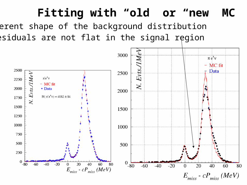
Fitting with “old” or “new” MCDifferent shape of the background distributionFit residuals are not flat in the signal region

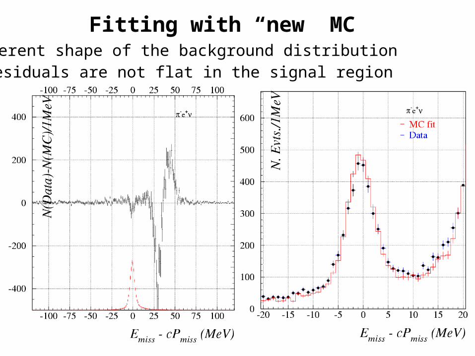
Fitting with “new” MCDifferent shape of the background distributionFit residuals are not flat in the signal region

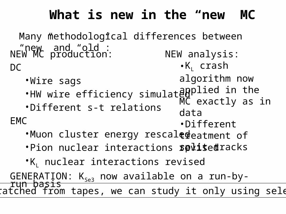
What is new in the “new” MC

Many methodological differences between “new” and “old”:

NEW analysis:•KL crash algorithm now applied in the MC exactly as in data•Different treatment of split tracks

NEW MC production:

DC•Wire sags•HW wire efficiency simulated•Different s-t relations

EMC•Muon cluster energy rescaled•Pion nuclear interactions revised•KL nuclear interactions revised

GENERATION: KSe3 now available on a run-by-run basis

OLD MC scratched from tapes, we can study it only using selected evts

Comparing “old” vs “new” MC

Background composition:• “” KS with before the DC• “” KS with bad reconstruction, tracking and/or TCL’s• “” KS with an hard , tails of TCL resolution• KS • KS

• Not KSKL events: , KK with a fake KL crash

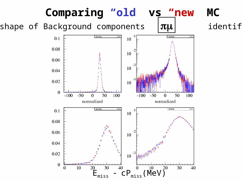
Comparing “old” vs “new” MCChecking shape of Background components identified as e

Emiss cPmiss(MeV)

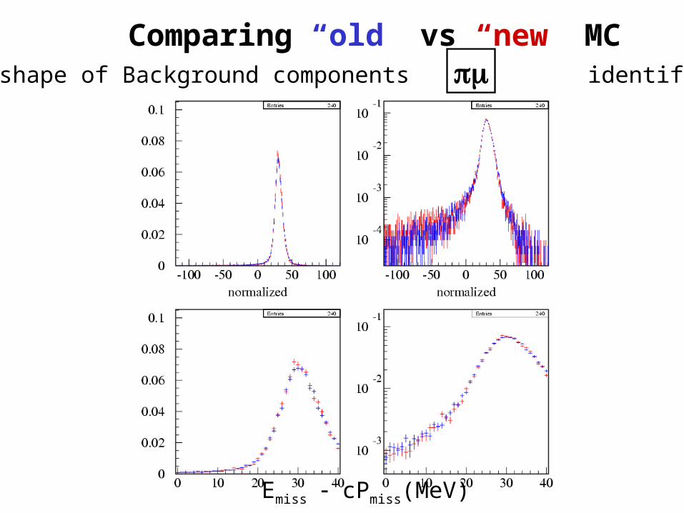
Comparing “old” vs “new” MCChecking shape of Background components identified as e

Emiss cPmiss(MeV)

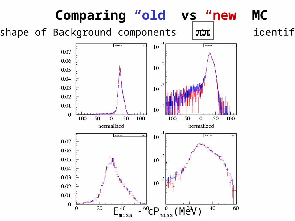
Comparing “old” vs “new” MCChecking shape of Background components identified as e

Emiss cPmiss(MeV)

Comparing “old” vs “new” MCChecking shape of Background components identified as e

Emiss cPmiss(MeV)

Comparing “old” vs “new” MCChecking shape of Background components identified as e

Emiss cPmiss(MeV)

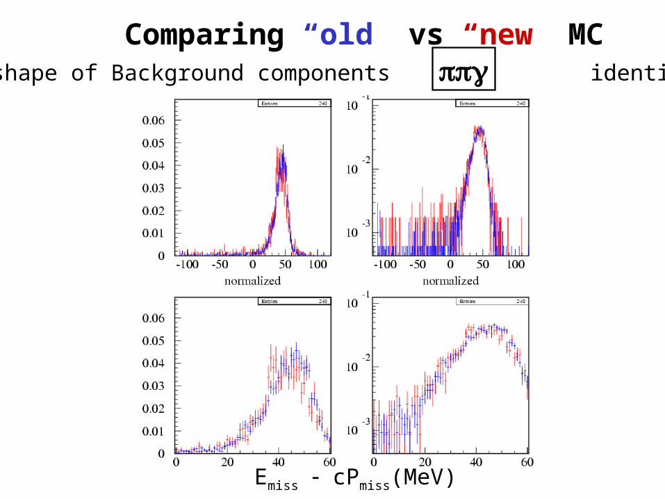
Comparing “old” vs “new” MCChecking shape of Background components identified as e

Emiss cPmiss(MeV)

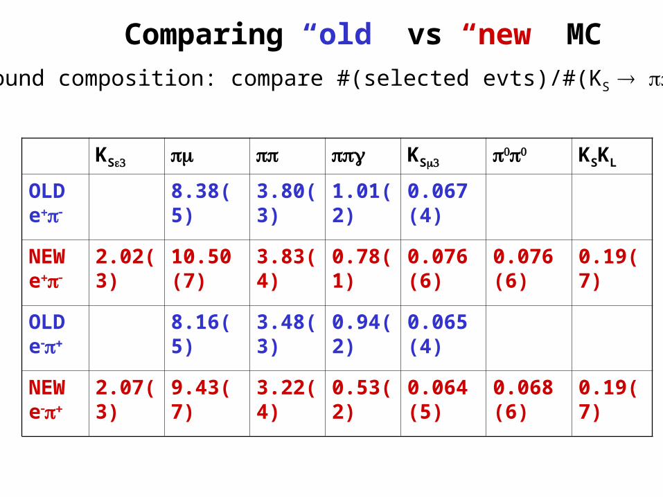
Comparing “old” vs “new” MC

Background composition: compare #(selected evts)/#(KS 104

KS KS KSKL

OLD e

8.38(5) 3.80(3) 1.01(2) 0.067(4)

NEW e

2.02(3) 10.50(7) 3.83(4) 0.78(1) 0.076(6) 0.076(6) 0.19(7)

OLD e

8.16(5) 3.48(3) 0.94(2) 0.065(4)

NEW e

2.07(3) 9.43(7) 3.22(4) 0.53(2) 0.064(5) 0.068(6) 0.19(7)

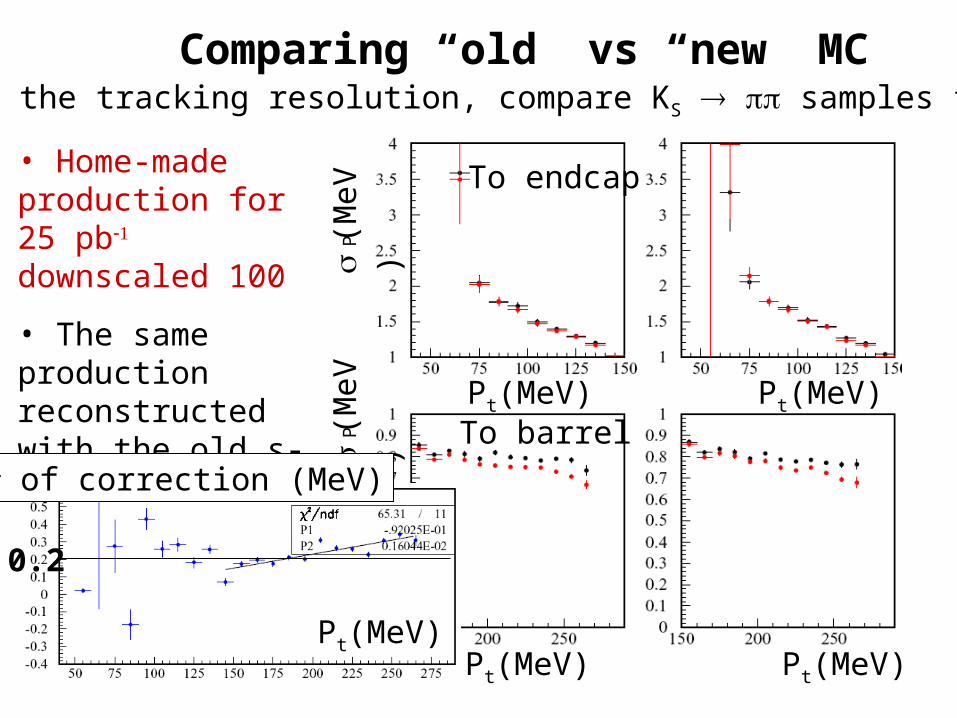
Comparing “old” vs “new” MCCore of the tracking resolution, compare KS samples from:

• Home-made production for 25 pb downscaled 100

• The same production reconstructed with the old s-t rel.

Pt(MeV)

Pt(MeV) Pt(MeV)

Pt(MeV)

P(M

eV)

P(M

eV)

Pt(MeV)

of correction (MeV)

0.2

To endcap

To barrel

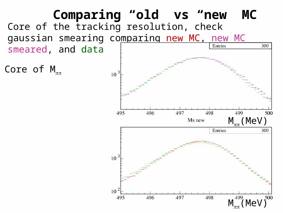
Comparing “old” vs “new” MCCore of the tracking resolution, check gaussian smearing comparing new MC, new MC smeared, and data

M(MeV)

M(MeV)

Core of M

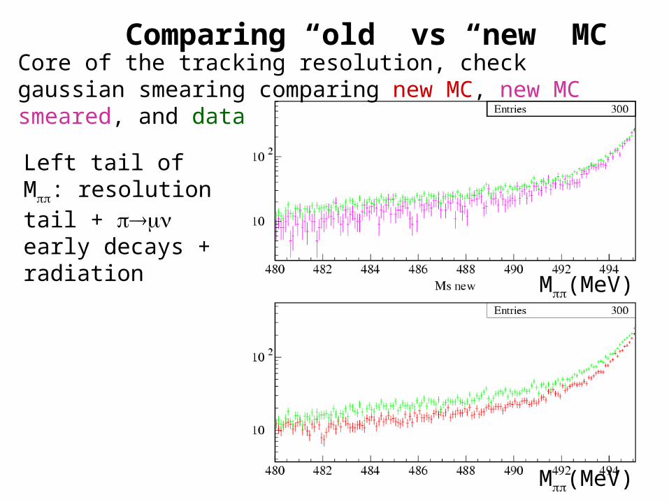
Comparing “old” vs “new” MCCore of the tracking resolution, check gaussian smearing comparing new MC, new MC smeared, and data

M(MeV)

M(MeV)

Left tail of M: resolution tail + early decays + radiation

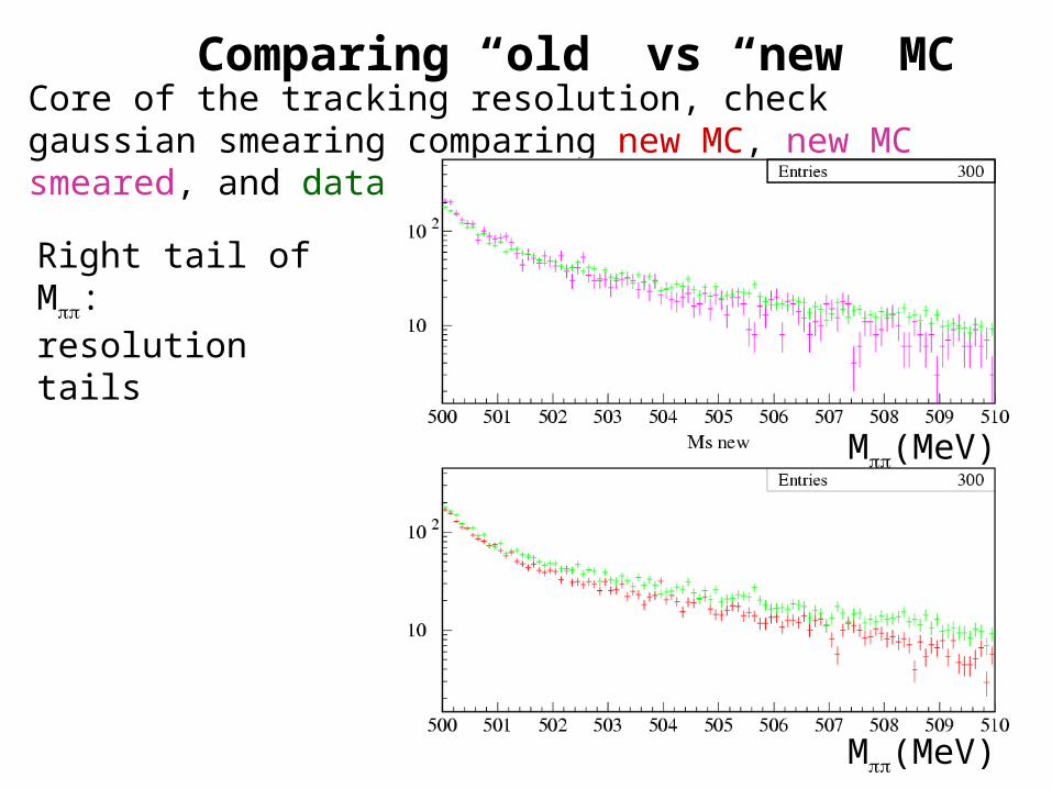
Comparing “old” vs “new” MCCore of the tracking resolution, check gaussian smearing comparing new MC, new MC smeared, and data

M(MeV)

M(MeV)

Right tail of M: resolution tails

Comparing data vs “new” MCKLe3 sample used to check the distribution for the signal:

• KS tight selection, 490<M<500 MeV, 100<p*<120 MeV• KS auto-triggering• Separation between KS and KL hemispheres• Estimate KL momentum from KS (different than the KL crash estimate)• Correct position of the KL vertex sampling from the KS lifetime, moves KL cluster positions accordingly • Apply the same cuts used for the KS analysis

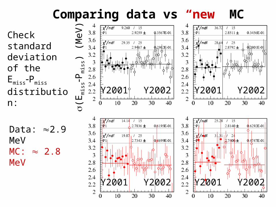
Comparing data vs “new” MC

Data: 2.9 MeVMC: 2.8 MeV

(E

mis

sPm

iss)

(M

eV)Check standard

deviation of the EmissPmiss distribution:

Y2001 Y2002

Y2001 Y2002 Y2001 Y2002

Y2001 Y2002

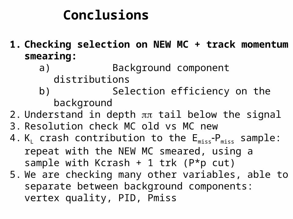
Conclusions

1. Checking selection on NEW MC + track momentum smearing:a) Background component distributionsb) Selection efficiency on the background

2. Understand in depth tail below the signal3. Resolution check MC old vs MC new4. KL crash contribution to the EmissPmiss sample: repeat with the NEW

MC smeared, using a sample with Kcrash + 1 trk (P*p cut)5. We are checking many other variables, able to separate between

background components: vertex quality, PID, Pmiss