steady laminar axisymmetrical nozzle flow at …annemie.vanhirtum/_publi/grandchamp... · vins...

X. Grandchamp

Y. Fujiso

B. Wu

A. Van Hirtum1

e-mail: annemie.vanhirtum@gipsa-lab.

grenoble-inp.fr

GIPSA-lab,

UMR CNRS 5216,

Grenoble University,

Grenoble, 38000 France

Steady Laminar AxisymmetricalNozzle Flow at ModerateReynolds Numbers: Modelingand ExperimentFlow through an axisymmetrical parameterized contraction nozzle of limited size witharea contraction ratio 21.8 and total length 6 cm is studied for moderate Reynolds num-bers 300<Re< 20,200. The transverse flow profiles at the nozzle exit are characterizedby hot film anemometry for two different spatial step sizes. The flow at the exit is laminarand uniform in its core. Boundary layer characteristics at the nozzle exit are estimatedfrom the transverse velocity profiles. Flow throughout the nozzle is modeled by imple-menting Thwaites laminar axisymmetrical boundary layer solutions in an iterative algo-rithm for which both universal functions, describing the shape factor and skin frictionparameters respectively, are altered by adding a constant. The value of the constants isdetermined by fitting the modified universal functions to tabulated values reported in Ble-vins (Blevins, R., 1992, Applied Fluid Dynamics Handbook. Krieger, Malabar, FL.). Themodel is validated on the measured data. Adding nonzero constants to the universal func-tions improves the prediction of boundary layer characteristics so that the range of Reyn-olds numbers for which the discrepancy with experimental findings is less than 4% isextended from Re> 3000 to Re> 1000. Therefore, the studied contraction nozzle is ofuse for applications requiring a small nozzle with known low turbulence flow at the exitsuch as moderate Reynolds number free jet studies or bio fluid mechanics (respiration,speech production,…) and the flow at the exit of the nozzle can be accurately describedby a simple boundary layer algorithm for Re> 1000. [DOI: 10.1115/1.4005690]

1 Introduction

Studies dealing with wind tunnel design are multiple and requireto study the influence of the upstream geometry on the flow charac-teristics at the inlet of a wind tunnel working section [1–9]. Besidescharacterization of the exit profile of the nozzle, corresponding tothe inlet portion to the working section, attention is given to avoidadverse pressure gradients along the nozzle walls in order to favorlow turbulence inflow to the working section. Despite the amountof available literature most of the cited studies focus on wind tunnelapplications in aeronautics so that even low-speed wind tunnelssuch as proposed in Ref. [4] are characterized by a typical exit di-ameter of 3 m and Reynolds number of 1.3� 107. Consequently,the nozzle design and associated flow conditions at the nozzle exitreported in literature need to be validated for axisymmetrical inletnozzles for which the exit diameter is of order of centimeters andfor which the working range is limited to moderate Reynolds num-bers of order 103. More recently, studies dealing with moderateReynolds number free axisymmetrical jet development issuingfrom a contraction nozzle suggest that the velocity profile at theexit exhibits the sought features of uniform core and low turbulencelevel [10,11]. Nevertheless a thorough validation is necessary sincethe mentioned studies (1) provide a poor description of the contrac-tion nozzle such as [10] where a contraction nozzle with exit diam-eter 4cm is mounted into a wall which is likely to alter results forReynolds numbers 850�Re� 6750 and/or (2) are limited to asmall range of Reynolds numbers such as in Ref. [11] where a sin-gle Reynolds number Re¼ 16,000 is experimentally assessed for anozzle with exit diameter 14 mm and/or (3) uses commerciallyavailable nozzles such as in Ref. [12] for which the design is fixed

and the smallest diameter is about 5 cm and for which flow featuresare not maintained for Reynolds numbers lower than Re� 6500.

Therefore, the current study aims to provide an axisymmetriccontraction nozzle geometry based on the elegant parameterizedgeometries developed for wind tunnels [3,4] and to quantify flowfeatures at the nozzle exit with respect to turbulence intensity anduniformity in the center. Those features are required as inlet condi-tions for experimental studies of free jets [10–12], aeroacoustics orbio fluid mechanics (respiration, speech production, whizzle,…).The mentioned examples of bio fluid mechanics are demandingsince airflow is characterized by Reynolds numbers Re< 20,200,Mach number <0.2 and characteristic dimensions which aresmaller than the smallest commercially available nozzle. Conse-quently, experimental validation of physical modeling of flow de-velopment and aeroacoustic noise production in relation to thevocal tract requires a tailored nozzle with known inlet conditionsfor low to moderate Reynolds numbers. Obviously, known inflowconditions can be simply obtained by inserting a pipe in the experi-mental setup in order to ensure fully developed Poiseuille flow.Nevertheless, for the aimed range of Reynolds numbers therequired pipe length results in a long experimental setup (orders ofmeters [13–15] compared to order of centimeters for the length ofan adult vocal tract [16–18]). In addition, pipe flow results in turbu-lence levels of 5% which is high compared to the level expected atthe exit of a contraction nozzle [10,11,19,20]. Consequently, pipeflow is not suitable in case a short nozzle with low turbulenceinflow is aimed. Instead, a short contraction nozzle is sought basedon the parameterized geometries and design criteria proposed inRefs. [3,4].

In order to quantify flow properties at the nozzle exit experimen-tally, the transverse velocity profile at the exit of the axisymmetri-cal contraction nozzle is measured by hot-film anemometry fromwhich the flow at the nozzle exit is characterized and boundarylayer characteristics are derived [19–22]. In addition, the influence

1Corresponding author.Contributed by Fluids Engineering Division for the JOURNAL OF FLUIDS ENGINEERING.

Manuscript received February 2, 2011; final manuscript received November 15, 2011;published online February 23, 2012. Assoc. Editor: Mark F. Tachie.

Journal of Fluids Engineering JANUARY 2012, Vol. 134 / 011203-1Copyright VC 2012 by ASME

Downloaded 01 Mar 2012 to 195.83.80.172. Redistribution subject to ASME license or copyright; see http://www.asme.org/terms/Terms_Use.cfm

of the transverse spatial step on the estimated boundary layer char-acteristics is assessed.

Besides an experimental validation it is sought to model the flowproperties at the nozzle exit and to validate the outcome on themeasured quantities. In addition, flow modeling can be used toassess the variation of geometrical nozzle parameters on the flowproperties at the nozzle exit and to describe the flow throughout thenozzle. Since a flow with uniform center and low turbulence inten-sity is aimed, it is appropriate to apply laminar boundary layertheory. A simple and accurate model [19,20,22] is provided byThwaites laminar axisymmetrical boundary layer solution [23–25].The accuracy of the model is further increased by implementationin an iterative algorithm. Thwaites method exploits a functionalrelationship between Thwaites parameter and the boundary layershape factor and skin friction parameter which varies as function offlow and geometrical conditions and is expressed either by tabu-lated values, e.g., [1] or by universal functions, e.g., [22]. Conse-quently, validation of the model results should take into accountdifferent functional relationships. In order to do so, it is proposed toalter the universal functions describing the shape factor and skinfriction parameter by adding a constant to each function. The valueof the constants is determined by fitting the modified universalfunctions to the tabulated values [1].

In the following, the nozzle geometry is motivated. Next,Thwaites laminar boundary layer solution is outlined, the modi-fied universal functions are introduced and the iterative algorithmis detailed. In the following section, the experimental setup isdescribed and the measured flow profiles at the nozzle exit arecharacterized. Next, the flow throughout the nozzle is modeledand experimental and modeled flow results are compared. Finally,main findings are summarized in the conclusion.

2 Nozzle Geometry

An axisymmetrical contraction nozzle is needed to provide airinflow with reduced turbulence level and uniformity [3,4,9].Moreover a small nozzle is preferred in order to facilitate the usein an experimental setup. The axisymmetrical contraction nozzlegeometry proposed in Ref. [3] is applied. The nozzle radius R(x)along the contraction is fully defined by two matched cubics as:

RðxÞ ¼ D1

2� D2

2

� �1� ðx=LÞ3

ðxm=LÞ2

!þ D2

2; x � xm (1)

RðxÞ ¼ D1

2� D2

2

� �1� x=Lð Þ3

ð1� xm=LÞ2þ D2

2; x > xm (2)

with x the main streamwise direction, matching point of the cubicsxm, inlet diameter D1, outlet diameter D2 and total nozzle lengthL. Consequently, the nozzle geometry is fully determined by fourgeometrical parameters (D1, D2, L, xm) compared to six parame-ters required for the contour nozzle proposed in Ref. [4]. The geo-metrical parameter set (D1, D2, L, xm) is equivalent to (D1,2, CR,L, xm) with CR denoting the area contraction ratio defined asCR¼ (D2/D1)2.

The exit diameter D2 is determined based on the aimed flowconditions of moderate Reynolds numbers 300<Re< 20,200 andlow Mach number <0.2. Consequently, characteristic lengths aresmaller than 20mm so that the outlet diameter D2 yields 20 to 25mm, 20�D2� 25 mm. From studies of the contraction ratio inrelation to the Reynolds number [3,4], it is known that large con-traction ratios are more tolerant to irregularities occurring for lowvelocities due to, e.g., flow separation. Therefore the inlet diame-ter D1 is set to D1¼ 100 mm resulting in a large area contractionratio 15�CR� 22. The total nozzle length is set to 0.6 times theinlet diameter D1 or L¼ 60 mm3. Due to the high contraction ratioCR a short outlet length is needed to avoid boundary layer thick-ening at the exit. Therefore, the matching point is chosen asxm¼ 52 mm, corresponding to xm¼ 0.86L, so that the outlet length

is less than 5 mm. The resulting nozzle geometry is illustrated inFig. 1 for geometrical parameters D1¼ 100 mm, D2¼ 25 mm,L¼ 60 mm, and xm¼ 52 mm.

3 Laminar Boundary Layer Flow Modeling

At moderate Reynolds numbers the region in which viscousforces are important is confined to a thin laminar boundary layer ad-jacent to the wall. The resulting boundary layer theory in presenceof a pressure gradient is described by the Von Karman momentumintegral equation for steady flows [19,20]. The development of thelaminar boundary layer on the walls of the contraction defined in theprevious section is estimated by Thwaites method to solve the mo-mentum integral equation for laminar, incompressible and axisym-metrical boundary layers [23–25]. Outside the boundary layer, theflow is described as an inviscid irrotational ideal fluid flow in achannel. In the following U(x) denotes the fluid flow velocity out-side the boundary layer and u(x, y) indicates the velocity in theboundary layer.

The flow in the contraction is modeled by calculation of thelaminar boundary-layer momentum thickness,

d2ðxÞ ¼ð1

0

uðx; yÞUðxÞ 1� uðx; yÞ

UðxÞ

� �dy (3)

as a function of downstream distance x with Thwaites equationusing quasi-similarity assumptions [19,24]:

d22ðxÞR2ðxÞU6ðxÞ � d2

2ð0ÞR2ð0ÞU6ð0Þ ¼ 0:45�

ðx

0

R2ðxÞU5ðxÞdx

(4)

where U(0), d2(0) and R(0) are the flow velocity, momentumthickness and radius at the nozzle inlet x¼ 0 and � the kinematicviscosity. The second term at the left hand side of Eq. (4) takesinto account initial conditions at x¼ 0.

Next, a dimensionless Thwaites parameter k is defined as

k ¼ � d22

�

@UðxÞ@x

(5)

from which a skin friction parameter S(k),

SðkÞ ¼ d2

UðxÞ@U

@y(6)

Fig. 1 Illustration of parameterized axisymmetrical nozzlegeometry, D(x) 5 2R(x), obtained from matching at x 5 xm anupstream cubic (1) (dashed line) and a downstream cubic(2) (thin full line) with parameters D1 5 100 mm, D2 5 25 mm,L 5 60 mm, and xm 5 52mm. The longitudinal x-axis corre-sponds to the main streamwise direction and the y-axis to thetransverse direction.

011203-2 / Vol. 134, JANUARY 2012 Transactions of the ASME


and boundary layer shape parameter H(k),

HðkÞ ¼ d1ðxÞd2ðxÞ

(7)

can be estimated and for which d1 denotes the displacementthickness,

d1ðxÞ ¼ð1

0

1� uðx; yÞUðxÞ

� �dy (8)

Note that since the wall shear stress is defined as s ¼ q�@U@y , with q

denoting the fluid density, also the following holds:

SðkÞ ¼ sd2

q�U(9)

Consequently, the wall shear stress can be derived from the skinfriction parameter S(k) which becomes zero at flow separation anddepends only on the dimensionless Thwaites parameter k.

The skin friction parameter S(k) and shape parameter H(k)reported in literature are derived from experimental data and pre-sented as tabulated values [1] or as universal Thwaites functions[22,26]. It is observed that a discrepancy exists between the tabu-lated and functional values [1,22,26]. Non zero constantscH¼ 0.35 and cS¼�0.02 need to be added to the universalThwaites functions [22,26] in order to accurately fit the tabulatedvalues reported in Ref. [1]. The accuracy of the fit is confirmed bythe coefficient of determination which yields 0.97. The resultingmodified universal Thwaites functions are

SðkÞ ¼ 1:8k2 þ 1:57kþ 0:22þ cS; 0 � k � 0:1 (10)

HðkÞ ¼ 5:24k2 � 3:75kþ 2:61þ cH (11)

SðkÞ ¼ 0:018k0:107þ k

þ 1:402kþ 0:22þ cS; �0:1 � k � 0 (12)

HðkÞ ¼ 0:0731

0:14þ kþ 2:088þ cH (13)

where the constants cH,S are introduced to account for differentflow and geometrical conditions. Moreover from the cited studiesit is seen that the constants can vary in the range 0� cH� 0.35and �0.02� cS� 0. Resulting values for H(k) and S(k) obtainedfrom the modified universal Thwaites functions for zero and non-zero constants cH,S are illustrated in Fig. 2.

Using nonzero constants (cH¼ 0.35 and cS¼�0.02) instead ofzero constants (cH,S¼ 0) is therefore seen to alter H and S signifi-cantly since H increases between 10 and 25% and S decreasesbetween 5% and 10%. Therefore, the constants directly influencethe underlying physics since accounting for the set of non zeroconstants in the modeling facilitates flow separation.

Therefore, the influence of two sets of constants cH,S, zero(cH,S¼ 0) and non zero (cH¼ 0.35 and cS¼�0.02), on the model-ing outcome is assessed for flow through the nozzle outlined in Sec.2. In addition, the model outcome will be compared to experimentaldata.

The equations outlined in this section are implemented in an iter-ative algorithm detailed in the flow chart given in appendix 6 whichis applied at each spatial position until the solution converges for kand U. Briefly, the velocity is initialised using the given volumeflow rate Q and geometrical radius R(x) from which a first estima-tion of the momentum thickness d2 is obtained so that the Thwaitesparameter k and the displacement thickness d1 can be estimated byusing the expression for H(k) given in Eq. (7). The velocity is thanre-estimated while accounting for the displacement thickness fromwhich the values of k and U are updated by relaxation and the shearstress s is estimated with the expression of S(k) in Eq. (6). In orderto increase the accuracy of the model approach, the procedure isrepeated until the retrieved values for U and k converges to within0.01%.

4 Experimental Setup and Flow Characterization

In order to validate the model outcome and to characterize thevelocity profile at the nozzle outlet, hot film anemometry meas-urements are performed at the exit. In the following the experi-mental setup and procedure are described and the measuredvelocity profiles are characterized.

4.1 Experimental Setup. The experimental setup is illus-trated in Fig. 3(a). It consists in an oil injected rotary screw com-pressor Copco GA7 with an integrated oil/water separator. Inaddition, liquid and solid particles as well as oil odors and vaporsare filtered (Copco & Beko DD17, PD17, QD17) out so that dryair with no oil particulates is delivered. In addition, the compres-sor is equipped with an air receiver of 300 l.

To avoid any resulting vibrations and flow disturbances, thecompressor [a] is isolated in a separated room. Downstream, apressure regulator [b] (Norgren type 11-818-987) and a manualvalve [c] are placed in order to reduce air pressure and preventpressure fluctuations during experiments. The pressure regulatoris connected with a thermal mass flow meter (TSI 4040) [d] via a

Fig. 2 Illustration of (a) H(k) for cH 5 0 (c 5 0) and cH 5 0.35 (c=0) and (b) S(k) for cS 5 0 (c 5 0) and cS 5 20.02 (c=0)

Journal of Fluids Engineering JANUARY 2012, Vol. 134 / 011203-3


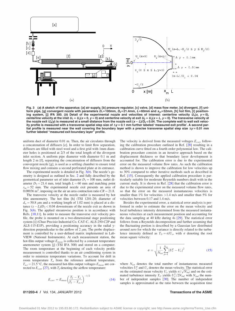
uniform duct of diameter 0.01 m. Then, the air circulates througha concatenation of diffusers [e]. In order to limit flow separation,diffusers are filled with steel wool and a first grid with 1mm diam-eter holes is positioned at 2/3 of the total length of the divergentinlet section. A uniform pipe diameter with diameter 0.1 m andlength 2 m [f], separating the concatenation of diffusers from theconvergent nozzle [g], is used as a settling chamber to ensure totalflow mixing and contains a second perforated plate at its entrance.

The experimental nozzle is detailed in Fig. 3(b). The nozzle’s ge-ometry is designed as outlined in Sec. 2 and fully described by thegeometrical parameter set of inlet diameter D1¼ 100 mm, outlet di-ameter D2¼ 21.4 mm, total length L¼ 60 mm and matching pointxm¼ 52 mm. The experimental nozzle exit presents an area of0.00036 m2, imposing on the air an area contraction ratio CR¼ 21.8.

The transverse velocity at the nozzle outlet is measured by hotfilm anemometry. The hot film [h] (TSI 1201-20; diameter ofdw¼ 50.8 lm and a working length of 1.02 mm) is placed at a dis-tance (x� L)/D2< 0.04 downstream of the nozzle exit as shown inFig. 3(b). The applied streamwise position is in accordance withRefs. [10,11]. In order to measure the transverse exit velocity pro-file, the probe is mounted on a two-dimensional stage positioningsystem [i] (Chuo Precisio Industrial Co. CAT-C, ALS-250-C2P andALS-115-E1P), providing a positioning accuracy in the radial y-direction perpendicular to the airflow of 2 lm. The probe displace-ment is controlled by a user-defined matrix implemented in Lab-VIEW (National Instruments). At each measurement station, thehot-film output voltage Emeas is collected by a constant temperatureanemometer system [j] (TSI IFA 300) and stored on a computer.The room temperature at the beginning of each velocity profilemeasurement is controlled thanks to an air conditioning system inorder to minimize temperature variations. To account for drift inroom temperature Ta from the reference ambient temperature,Ta,r¼ 21.5 �C, the measured hot-film output voltages Emeas are cor-rected to Ecorr [27], with Tf denoting the airflow temperature:

Ecorr ¼ EmeasTf � Ta

Tf � Ta; r

� ��1=2

(14)

The velocity is derived from the measured voltages Ecorr follow-ing the calibration procedure outlined in Ref. [28] resulting in acalibration curve fitted on a fourth order polynomial law. The cali-bration procedure consists in an iterative approach based on thedisplacement thickness so that boundary layer development isaccounted for. The calibration error is due to the experimentalerror on the measured volume flow rates. As such the calibrationmethod is shown to improve the calibration for low velocities upto 30% compared to other iterative methods such as described inRef. [15]. Consequently the applied calibration procedure is par-ticularly suitable for moderate Reynolds numbers dealt with in thecurrent study. It is shown in Ref. [28] that the calibration error isdue to the experimental error on the measured volume flow rates,so that the error on the measured instantaneous velocities issmaller than 1% for velocities >1.4 m/s and smaller than 5% forvelocities between 0.17 and 1.4 m/s.

Besides the experimental error, a statistical error analysis is per-formed in order to estimate the error on the mean velocity andlocal turbulence intensity determined from the measured instanta-neous velocities at each measurement position and accounting forthe data sampling at 40 kHz during 4s [29]. The statistical errorfollows from a Reynolds decomposition and further assuming thatthe fluctuating portion is described by a Gaussian law distributedaround zero for which the variance is directly related to the turbu-lence intensity defined as TU¼r/Ue, with r denoting the rootmean square velocity:

r ¼

ffiffiffiffiffiffiffiffiffiffiffiffiffiffiffiffiffiffiffiffiffiffiffiffiffiffiffiffiffiffiffiffiffiffiffiffiffi1

Ntot

XNtot

p¼1

Upe � Ueð Þ2

vuut (15)

where Ntot denotes the total number of instantaneous measuredvelocities Up

e and Ue denotes the mean velocity. The statistical erroron the estimated mean velocity Ue yields r=

ffiffiffiffiffiffiffiffiNind

pand on the esti-

mated turbulence intensity TU yields U2e=2Nind with Nind the num-

ber of independent samples [30]. The number of independentsamples is approximated as the ratio between the acquisition time

Fig. 3 (a) A sketch of the apparatus: [a] air supply, [b] pressure regulator, [c] valve, [d] mass flow meter, [e] divergent, [f] uni-form pipe, [g] convergent nozzle with parameters D15100mm, D2521.4mm, L560mm and xm552mm, [h] hot film, [i] position-ing system, [j] IFA 300. (b) Detail of the experimental nozzle and velocities of interest: centerline velocity Uc(x, y 5 0),centerline velocity at the inlet U1 5 Uc(x 5 0, y 5 0) and centerline velocity at exit U2 5 Uc(x 5 L, y 5 0). The transverse velocity atthe nozzle exit Ue(y) is measured at a small distance from the nozzle exit (x 2 L)/D2 < 0.04. The complete wall to wall exit veloc-ity profile is measured with a transverse spatial step size of Dy 5 0.1 mm further labeled ‘measured exit profile’. A second par-tial profile is measured near the wall covering the boundary layer with a precise transverse spatial step size Dy 5 0.01 mmfurther labeled “measured exit boundary layer” profile.



of 4s and the integral time � D2=Ue, i.e., Nind � 8Q=pD32. The

resulting statistical errors for an assumed turbulence level of 2% issmaller than the experimental measurement error. It is shown in thefollowing section, Fig. 5, describing the measured velocity profiles,that 2% overestimates the measured turbulence level along thecenterline at the exit. Therefore, the measurement error on the vol-ume flow velocity is the main error source in the performedmeasurements.

All used instruments, their corresponding uncertainties and theerror estimations on the measured velocity and statistical quanti-ties are summarized in Table 1.

4.2 Measured Velocity Profiles at the Nozzle Exit. Trans-verse flow characteristics at the nozzle exit are measured by plac-ing the probe at the horizontal centerline of the jet at a distance(x�L)/D2< 0.04 and displacing the probe in the transverse direc-tion as schematically illustrated in Fig. 3(b). The streamwise posi-tioning (x� L)/D2< 0.04 in order to measure the transverse flowat the nozzle exit is commonly used in literature, e.g. (x� L)/D2< 0.04 in [10] or (x� L)/D2¼ 0.05 in Ref. [11]. Volume flowrates are varied in the range 5<Q< 305l/min, which corresponds

to Reynolds numbers 300<Re< 20,200 with Re the Reynoldsnumber based on the bulk velocity at the nozzle exit, i.e.,Re¼ 4Q/�p D2.

For each Reynolds number two transverse profiles are measuredwith different spatial step sizes. The spatial step sizes are chosenrelative to the hot film diameter, dw¼ 50.8 lm � 0.05 mm, since itis expected that the accuracy of the step size relative to the sensordiameter will affect the accuracy of the numerical integrationrequired in order to determine the boundary layer characteristics atthe nozzle exit such as d1 and d2 defined in Eq. (8) and Eq. (3).Firstly, the transverse exit profile is measured from wall to wall,�0.5� y/D2< 0.5, with a transverse spatial step equal toDy¼ 0.1mm, i.e., Dy> dw since Dy � 2dw, further labeled“measured exit” profile. Secondly, a boundary layer profile is meas-ured with a spatial step Dy¼ 0.01 mm, i.e., Dy< dw since Dy � dw/5, further labeled “measured exit boundary layer” profile. Finally, itis remarked that the spatial step size used to measure the transverseexit profile is not mentioned in the cited studies [10,11].

Measured velocity profiles obtained with spatial steps Dy¼ 0.1mm and Dy¼ 0.01 mm are illustrated in Fig. 4(b) for �0.5�R/D2��0.3.

Table 1 Relevant measurement range and corresponding uncertainties of instruments. Upper limits of uncertainties for measuredinstantaneous velocities and estimated statistical errors for the first and second velocity moments [28–30] for sampling at 40kHzduring 4s. Statistical errors are estimated assuming 2% turbulence level, i.e., TU 5 2%.

Instruments

Quantity Symbol Instrument Relevant measurement range Uncertainty

Flow rate Q TSI model 4040 5–305 l/min 62%Fluid temperature Tf TSI model 4040 20–25 �C 61 �CRoom temperature Ta OTAX 421001 22–25 �C 60.2 �CNozzle exit diameter D2 Manufacturing precision 21.4 mm 60.02 mmFluid pressure Pf TSI model 4040 97–115 kPa 61 kPaData acquisition Emeas PCI-MIO-16XE-10 (National Instruments)

and IFA300 (TSI)610V 672.3lV

Transverse positioning Dy CHUO Precisio 0.1 mm and 0.01 mm 60.002 mm

Velocities

Velocity Symbol Error Relevant range Uncertainty

Instantaneous velocity Up measurement error on Q > 1.4m/s < 1%Mean velocity Ue > 0.17m/s and< 1.4m/s < 5%Root mean square velocity r < 0.17m/s > 5%

Fig. 4 (a) Comparison of measured exit velocity profiles Ue(y) obtained with spatial step Dy 5 0.1 mm (symbols) and meas-ured exit boundary layer profiles Dy 5 0.01 mm (dots) for different Reynolds numbers Re in the range 20.5 £ R/D2 £ 20.3. (b)Measured normalized transverse exit velocity profiles Ue(y)/U2 for Dy 5 0.1mm and comparison with parabolic, 1/7 power law,uniform profile with vanishing momentum thickness d2 5 0 and top hat profile with momentum thickness d2 5 0.004D2.



The measured velocity profiles match well for all assessedReynolds numbers illustrating that no error is due to the position-ing of the hot film at (x� L)/D2< 0.04.

Normalized mean exit velocity profiles Ue(y)/U2 with U2 theexit centerline velocity, are illustrated in Fig. 4(b). The measuredexit profiles are compared to a parabolic velocity profile describ-ing fully developed pipe flow in Eq. (16), a 1/7 power law profiledescribing turbulent flow in Eq. (17), a theoretical uniform profilecorresponding to a top hat velocity profile in Eq. (18) with vanish-ing momentum thickness d2¼ 0 [31] and a top hat profile account-ing for boundary layer development with momentum thicknessd2¼ 0.004D2:

Ue ¼ U2 1� 2jyjD2

� �2 !

(16)

Ue ¼ U2 1� 2jyjD2

� �1=7

(17)

Ue ¼1

2U2 1� tanh

D2

8d2

2jyjD2

� D2

2 yj j

� �2 ! !

(18)

For all assessed Reynolds numbers the variation in mean velocityis lower than 0.5% in the center portion of the jet jyj=D2 < 0:25.The top hat profile describes well the uniform flow in the constantvelocity center region as well as the boundary layer region in casea non vanishing momentum thickness is accounted for d2 6¼ 0.Nevertheless, it is seen that the boundary layer thickness increasesrapidly for Re< 3000. For Reynolds numbers Re> 3000 the con-stant velocity region is extended to jyj=D2 < 0:4 in accordancewith observations described by Ref. [10,11]. A small overshoot inthe outer part of the core of the mean exit velocity profiles isobserved. The overshoot is of the order of magnitude reported inRef. [11] and smaller than the overshoot observed in Ref. [10].The contraction nozzle studied by Ref. [10] has no outlet length,i.e., nozzle outlet for which the nozzle is parallel with the center-line, which causes the vena contracta effect to be more pro-nounced in the exit profile. The overshoot might also be effecteddue to differences in contraction ratio. The contraction ratios inthe current study and in Ref. [11] are of the same order of magni-tude whereas information on the contraction ratio of the nozzleused in Ref. [10] is missing.

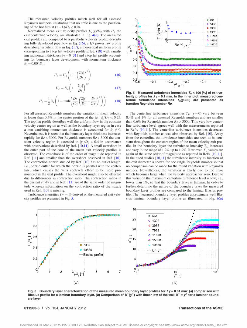
Turbulence intensities TU ¼ rU2

derived on the measured exit velo-city profiles are presented in Fig. 5.

The centerline turbulence intensities TU (y¼ 0) vary between0.4% and 1% for all assessed Reynolds numbers and are smallerthan 0.6% for Reynolds number Re> 3000. This very low center-line turbulence level agrees well with the measurements reportedin Refs. [10,11]. The centerline turbulence intensities decreaseswith Reynolds number as was also observed by Ref. [10]. Awayfrom the centerline the turbulence intensities are seen to be con-stant throughout the constant region of the mean velocity exit pro-file. In the boundary layer the turbulence intensity TU increasesand vary in the range of 1.2% up to 1.9%. Retrieved TU values areagain of the same order of magnitude as reported in Refs. [10,11].In the cited studies [10,11] the turbulence intensity as function ofthe exit diameter is shown for one single Reynolds number so thatno comparison can be made for the found variation with Reynoldsnumber. Nevertheless, the variation is likely due to the errorwhich becomes large when the velocity approaches zero. Despitethis variation the maximum centerline turbulence level is low, i.e.,lower than 1%, so that the boundary layer is laminar. In order tofurther determine the nature of the boundary layer the measuredboundary layer profiles are compared to the laminar Blasius pro-file. The measured boundary layer profiles approximate well Bla-sius laminar boundary layer profile as illustrated in Fig. 6(a)

Fig. 5 Measured turbulence intensities TU 3 100 [%] of exit ve-locity profiles for Dy 5 0.1 mm. In the inner plot, measured cen-terline turbulence intensities TU(y 5 0) are presented asfunction Reynolds number Re.

Fig. 6 Boundary layer characterization of the measured mean boundary layer profiles for Dy 5 0.01 mm: (a) comparison withBlasius profile for a laminar boundary layer. (b) Comparison of U1(y1) with linear law of the wall U1 5 y1 for a laminar bound-ary layer.



confirming the laminar nature of the boundary layer [19,20]. Inaddition, in Fig. 6(b) the measured boundary layer profiles areseen to be in very good agreement with a linear law of the walldefined as Uþ¼ yþ with Uþ denoting the velocity normalized bythe friction velocity Us ¼

ffiffiffiffiffiffiffiffis=q

pand yþ indicating the Reynolds

number based on the friction velocity Us and distance from thewall, i.e., yþD/2 [20,22,32].

So from the measured velocity profiles, it is observed that theflow at the nozzle exit is laminar and the boundary layer is seen tobe confined to the vicinity of the wall for all assessed Reynoldsnumbers Re so that the mean velocity profile has a satisfactorysharp top-hat shape.

5 Nozzle Flow: Modeling and Experiment

In the current section flow through an axisymmetrical nozzle isdiscussed for Reynolds numbers in the range 300<Re< 20,200.The flow through the nozzle is modeled following the laminarboundary layer method outlined in Sec. 3. The model outcome isdiscussed in Sec. 5.1. Next, the influence of geometrical andmodel parameters on the modeled centerline velocity at the nozzleexit is assessed in Sec. 5.2. In addition, modeled and measuredcenterline velocities at the exit of the nozzle are compared.Finally, the experimental validation of boundary layer characteris-tics at the nozzle exit is presented in Sec. 5.3.

5.1 Modeled Streamwise Nozzle Flow. The flow through anaxisymmetrical nozzle is modeled following the laminar boundarylayer method outlined in Sec. 3. The constants cH,S introduced inthe modified universal Thwaites functions defined in Eq. (13) areset to zero so that cH¼ 0 and cS¼ 0. The nozzle geometryA(x)¼ pR(x)2 is obtained as outlined in Sec. 2 and consequentlyfully defined by the parameter set (D1, D2, L, xm) composed out ofinlet diameter D1, outlet diameter D2, total nozzle length L andstreamwise position of matching point xm. In the current sectionthe parameter set is fixed to the values corresponding to the exper-imental nozzle: D1¼ 100 mm, D2¼ 21.4 mm, L¼ 60 mm, andxm¼ 52 mm. The influence of non zero constants on the modeloutcome and of varying geometrical nozzle parameters on themodeled flow outcome at the nozzle exit is discussed in Sec. 5.2.The modeled streamwise flow quantities for Reynolds numbers inthe range 300<Re< 20,200 are illustrated in Fig. 7.

The modeled mean streamwise centerline velocities normalizedby the inlet velocity, Uc/U1, are illustrated in Fig. 7(a). The cen-terline velocity increases in the streamwise direction until a maxi-mum is reached at the nozzle exit. As a benchmark the modeledcenterline velocity is compared to the bulk velocity, defined as theratio of volume flow rate Q and area A(x), corresponding to anideal fluid for which boundary layer development is neglectedwhich results in U(x)/U1¼Ax¼ 0/A(x). Consequently, the normal-ized bulk velocity depends only on the geometry and not on theReynolds number Re. At the nozzle outlet the bulk velocity equalsthe area contraction ratio CR. From Fig. 7(a) is seen that the nor-malized modeled centerline velocity profiles collapse to a singlecurve for Re> 3000. For Reynolds numbers Re< 3000 on theother hand the ratio Uc/U1 increases throughout the nozzle due toan increased flow acceleration for Re< 3000 as shown in Fig. 7(b)where the streamwise normalized flow acceleration dUc/dx�D1/U1 is plotted. The flow is accelerated due to the contraction geom-etry. Downstream the nozzle inlet, the flow accelerates graduallyuntil a maximum acceleration is reached just downstream thematching point xm. The position of maximum flow acceleration isdefined by the geometry and independent from the Reynolds num-ber Re. Downstream the maximum flow acceleration the flowacceleration reduces until the nozzle exit. As expected from thecenterline velocity, the acceleration of all assessed Reynolds num-bers collapses except for Re< 3000. The reduced flow accelera-tion is causing increased boundary layer development for lowReynolds numbers as was observed experimentally on the meanexit velocity profiles shown in Fig. 4(a) since a decrease of

velocity leads to an increase of the viscous effects and conse-quently boundary layer thickening. Consequently, values charac-terizing the boundary layer such as the displacement thickness d1

and the momentum thickness d2 are expected to decrease as theReynolds number increases.

The displacement thickness d1 normalized by the exit diameterD2 is shown in Fig. 7(c). It is observed that the boundary layerdevelops in the almost uniform inlet section of the nozzle result-ing in an increase of the displacement thickness d1. The displace-ment parameter d1 increases to 10% of the exit diameter D2,corresponding to 2% of the inlet diameter D1 for Re> 3000. ForReynolds numbers Re< 3000 the increase of d1 is more pro-nounced yielding 25% the exit diameter D2 or 5% of the inlet di-ameter D1. At the onset of the contraction d1 decreases due to theflow acceleration in the streamwise direction towards the match-ing point xm imposing an increased flow velocity which reducesviscous effects and so the growth of the boundary layer. A mini-mum is reached at the point of maximum flow acceleration whichis easily identified from Fig. 7(b). For all Reynolds numbers thedisplacement thickness is less than 3% at the streamwise locationcorresponding to maximum flow acceleration and less than 0.5%for Re> 3000. Downstream the point of maximum flow accelera-tion, the flow acceleration reduces towards the nozzle exit due tothe reduced rate of area change. This results in a velocity reduc-tion which is associated with an increase of viscous effects and soa boundary layer thickening. As a consequence, boundary layerparameters d1,2 increase towards the nozzle exit. At the nozzleexit the discplacement thickness d1 yields less than 1% of the exitdiameter D2 for Re> 3000. For smaller Reynolds numbersRe< 3000, the displacement thickness d1 increases to 4% of theexit diameter D2.

The normalized momentum thickness d2/D2 is shown in Fig.7(d). Comparing d1/D2 shown in Fig. 7(c) to d2/D2 represented inFig. 7(d) shows that the tendencies outlined for the normalizeddisplacement thickness d1/D2 also apply to the normalized mo-mentum thickness d2/D2, except that the magnitude of d2 isreduced compared to the magnitude of d1. The ratio of d1 and d2,which corresponds to the shape factor H following Eq. (7), isshown in Fig. 7(e). For all assessed Reynolds numbers Re, theshape factor at the nozzle inlet yields H¼ 2.96, which is associ-ated with a laminar flow. The shape factor H is seen to decreasethroughout the nozzle with less than 0.5% so that 2.96�H� 2.95holds throughout the nozzle. Consequently, streamwise variationof the boundary layer shape factor H � 2.95 is limited which is inaccordance with the flow uniformity aimed for by using a contrac-tion nozzle. The observed decrease in the shape factor withincreasing Reynolds number Re is less than 0.05% which is of nosignificance when accounting for a model error and is of no signif-icance with respect to the total range of the shape factor shown inFig. 2. Therefore, the influence of Reynolds number on the bound-ary layer shape factor can be neglected.

From Eq. (7) is seen that the shape factor H(k) is only functionof the Thwaites parameter k. Consequently, an almost constantvalue of H(k) throughout the nozzle suggests an almost constantvalue for the skin friction parameter S(k), defined in Eq. (6), andsuggests an almost constant value for the Thwaites parameter kdefined in Eq. (5). From Fig. 7(g) is seen that the skin friction pa-rameter at the nozzle inlet yields S¼ 0.2 and increases throughoutthe nozzle with less than 3% so that 0.2� S� 0.205 holdsthroughout the nozzle. Consequently, streamwise variation of theskin friction parameter S � 0.2 is indeed limited. The small varia-tion of S as function of Reynolds number at the nozzle exit issmaller than 0.5% which is of no significance when accountingfor a model error and is of no significance with respect to the totalrange of the skin friction parameter shown in Fig. 2. Since S> 0for all streamwise positions it is observed that the flow remainsattached to the nozzle walls for all streamwise positions so that noflow separation occurs. Therefore, the proposed nozzle enablesflow uniformity at the nozzle exit and no flow separation occursupstream the nozzle exit. In accordance with the observations for



the shape factor H(k) and the skin friction parameter S(k) the vari-ation of the Thwaites parameter k throughout the nozzle, shown inFig. 7(e), can be neglected so that k � 0.0015 holds for all stream-wise positions and for all assessed Reynolds numbers.

The wall shear stress s is estimated following Eq. (9) ass¼ S(k)�qUc/d2. The physical fluid properties q and � are con-stant and the skin friction parameter S(k) can be approximated bythe constant value S � 0.2 regardless the Reynolds number.

Fig. 7 Illustration of modeled streamwise flow development through the contraction nozzlewith parameters D15100 mm, D2521.4 mm, L560 mm and xm552 mm, corresponding to areacontraction ratio CR 5 21.8, for cH 5 0 and cS 5 0 as function of different Reynolds numbers inthe range 300 £ Re £ 17,000 (symbols). The vertical dashed-dotted line indicates the matchingpoint of the cubics x 5 xm. The scaled radius of the nozzle is indicated by a solid thick line.



Consequently, estimated values for s are proportional to the ratioof the modeled centerline velocity Uc and the momentum thick-ness d2 since both quantities depend on the streamwise position xas well as on the Reynolds number Re as seen from Fig. 7(a) andFig. 7(d). The estimated wall shear stress s normalized by thepressure difference due to the contraction assuming an ideal fluidDP:

DP � q2

U21 CR2 � 1� �

(19)

� q�2

2

Re2

D22

1� 1

CR2

� �(20)

is shown in Fig. 7(h). The maximum wall shear stress is seen tooccur at a streamwise position located between the position of max-imum acceleration and the nozzle exit where the streamwise veloc-ity is maximum. For all assessed Reynolds numbers it is observedthat the estimated wall shear stress is of the same order of magni-tude as the pressure difference imposed by the contraction since thenormalized wall shear stress varies between 0.5 and 5.5. For Reyn-olds numbers in the range Re> 6000 the pressure difference ismore important than the wall shear stress as seen from 0.5< s/DP< 1. For Reynolds numbers 3000<Re< 6000 the normalizedwall shear stress increases in the range 1< s/DP< 2. For Reynoldsnumbers Re< 3000 the ratio increases further so that s/DP> 2holds indicating that viscous fluid forces becomes predominant,which is in accordance with the findings described for the centerlinevelocity Uc, the displacement thickness d1 and the momentumthickness d2. Moreover, it is noted that although the variation in themagnitude of the shape factor H(k) and the skin friction parameterS(k) are to small to be significant, the observed tendencies, i.e.,increase of H and decrease of S for decreasing Reynolds number,are in accordance with the loss of relative importance of the pres-sure gradient DP to the wall shear stress s.

5.2 Modeled and Measured Exit Centerline Velocity. InSec. 5.1 the modeled flow throughout the nozzle is described. Themodeled quantities show that a contraction nozzle with area con-traction ratio CR¼ 21.8 defined by the geometrical parameter setD1¼ 100 mm, D2¼ 21.4 mm, L¼ 60 mm, and xm¼ 52 mm ena-bles to obtain flow uniformity at the nozzle exit while flow separa-tion upstream the nozzle exit is avoided. In the current section theinfluence of the nozzle diameters (D1, D2) on the model outcomeis sought for fixed values of the total nozzle length L¼ 60 mmand the matching point xm¼ 52 mm. The assessed nozzle diame-ters (D1, D2) and corresponding area contraction ratio CR arelisted in Table 2. It is seen that all assessed contraction ratios sum-marized in Table 2 are smaller than or of the same order of magni-tude than CR¼ 21.8 for which no flow separation occurs. Since

flow separation is favored by increasing the contraction ratio, it isassumed that no flow separation occurs for any of the geometriessummarized in Table 2. The chosen values of D1, D2 and CR ena-ble to assess the influence of each individual parameter of the set(D1, D2, CR) on the modeled flow outcome.

Modeled centerline velocities at the nozzle exit U2 normalizedby the centerline velocity at the nozzle inlet U1, i.e., U2/U1, for allassessed nozzle parameters are shown in Fig. 8. In addition, meas-ured centerline velocities presented in Sec. 4 are plotted so that,for the nozzle characterized by the parameter set D1¼ 100 mm,D2¼ 21.4 mm, L¼ 60 mm, and xm¼ 52 mm, modeled and meas-ured values can be compared.

Figure 8(a) shows the influence of a variation of exit diameterD2 for a fixed upstream diameter D1¼ 100mm on the ratio of exitand inlet centerline velocity U2/U1 as function of Reynolds num-ber. The exit diameter D2 is varied in the range from 21.2 to 25mm corresponding to a variation of 10%. For an ideal fluid char-acterized by an uniform velocity profile throughout the nozzle, theratio U2/U1 yields the area contraction ratio, i.e. U2/U1¼CR,which is determined by the geometry and independent of Reyn-olds number. From Fig. 8(a) is seen that the variation of the ratioU2/U1 becomes indeed smaller than 1% for Reynolds numbersRe> 3000. For Reynolds numbers Re< 3000 the boundary layerdevelops rapidly so that the ratio U2/U1 increases in accordancewith observations made on Fig. 7(a). The ratio U2/U1 decreases asthe exit diameter D2 increases due to the decrease in contractionratio CR. Modeled and measured velocity ratios U2/U1 are com-pared for D2¼ 21.4mm. The modeled U2/U1 ratios matches wellwith the measured U2/U1 values except for Reynolds numbersRe< 3000 in which case the modeled values underestimate themeasured velocity ratios. The discrepancy between modeled andmeasured values increases from 1% for Re � 3000 to 20% forRe< 1000. Consequently, the applied model with parameterscH,S¼ 0 looses accuracy as the boundary layer growths forRe< 3000 and becomes inaccurate for Re< 1000.

The influence of varying inlet diameter D1 or exit diameter D2

on the velocity ratio U2/U1 for different Reynolds numbers is dis-cussed from Fig. 8(a) and Fig. 8(b). The geometrical parameterscharacterizing the experimental nozzle, D1¼ 100 mm andD2¼ 21.4 mm resulting in CR¼ 21.8, are taken as a reference.From Fig. 8(a) is seen that increasing the downstream diameterD2 with 61% and 17% decreases the predicted velocity ratio U2/U1 with 63% and 27%, respectively. From Fig. 8(b) is observedthat reducing the inlet diameter D1 with 50% and maintaining avariation of the upstream diameter D2 with 1% and 17% from itsreference value, reduces the influence of varying the downstreamdiameter D2 from its reference value to 1% and 12%. Conse-quently, the influence of a variation in exit diameter D2 on themodel outcome increases as the inlet diameter D1 increases.Moreover, it is seen that reducing the inlet diameter D1¼ 100 mmwith 50%, which corresponds to dividing the contraction ratio CRby 4, decreases the ratio U2/U1 by a factor greater than 4 or adecrease >25% illustrating the influence of reduced flow accelera-tion as the contraction ratio decreases.

In Fig. 8(a) and Fig. 8(b) the nozzle parameter D2 is variedwith 61% for a fixed value of D1¼ 100 mm so that a small varia-tion of 2% on the area contraction ratio CR is imposed. Figure8(c) shows the model outcome U2/U1 for the same variation of1% on the exit diameter D2 and a constant area contraction ratioCR¼ 4.5 which is obtained by increasing the inlet diameter D1

with less than 1%. From Fig. 8(c) is seen that the increase in inletand outlet diameter results in an increase of 1% in the ratio U2/U1

for all Reynolds numbers Re which is also observed in Fig. 8(b) incase only the exit diameter D2 is increased. Consequently, smallvariations <1% of the inlet diameter D1 do not influence themodel outcome for U2/U1.

Figure 8(d) shows the influence of the model parameters cH,S onthe model outcome as function of Reynolds numbers. The modelconstants are introduced in Eq. (7) for the boundary layer shape fac-tor H(k) and in Eq. (6) for the skin friction parameter S(k) in order

Table 2 Overview of varied parameters for contraction geome-tries defined in Eq. (1) and Eq. (2) for fixed matching positionxm 5 52 mm and contraction length L 5 60 mm: (I) constant inletdiameter D1, (II) constant outlet diameter D2, (III) constant con-traction ratio CR and (IV) geometrical nozzle parameters usedfor experimental validation as detailed in Sec. 4

D1 [mm] D2 [mm] CR [�]

Modeled I (D1) 100 21.2 22.2100 21.4 21.8100 21.6 21.4

II (D2) 100 25 1650 25 450 21.6 5.4

III (CR) 50 21.4 5.545.4 21.4 4.545.8 21.6 4.5

Experimental validation 100 21.4 21.8



to determine their dependence on the Thwaites parameter k. Thenozzle geometry is characterized by the reference values for the ge-ometrical parameters, D1¼ 100 mm and D2¼ 21.4 mm and there-fore CR¼ 21.8, corresponding to the nozzle used for experimentsdescribed in Sec. 4. The model outcome obtained for zero modelparameters cH,S¼ 0 is compared to the model outcome obtained fornon zero model parameters cH,S= 0. The choice of non zero modelparameters cH¼ 0.35 and cS¼�0.02 is motivated in Sec. 3. Forcompleteness also the constant value U2/U1¼CR is shown in Fig.8(d) which provides an underestimation of a boundary layer modelsince it assumes an ideal fluid characterized by a uniform velocityprofile for which boundary layer development is neglected. FromFig. 8(d) is seen that the influence of zero or non zero constantscH,S on the model outcome can be neglected for Reynolds numbersRe> 6000 for which the discrepancy between the modeled valuesis less than 1%. As the Reynolds number is decreased the discrep-ancy increases to <3% in the range 6000>Re> 3000 and up to15% for 3000>Re> 300. Consequently, the choice of model pa-rameters cH,S determines the model outcome in the range 300<Re< 3000. In order to evaluate the choice of model parameters cH,S

for the experimentally studied nozzle the model outcome is com-pared to the measured values for U2/U1. For Reynolds numbersRe> 3000 both zero and non zero model constants approximate themeasured data to within 2% corresponding with the experimental

error on the ratio U2/U1. For Reynolds numbers in the range3000>Re> 1000 the accuracy of the model outcome reduces towithin <7% for the use of zero constants and to within <4% forthe use of non zero constants cH,S= 0. For Reynolds numbersRe< 1000 the difference between measured and modeled U2/U1

ratios increases to more than 20% so that the model outcome isinaccurate for all assessed cH,S values.

5.3 Modeled and Measured Boundary Layer Characteris-tics at the Nozzle Exit. In the previous Sec. 5.2 the influence ofgeometrical parameters, inlet diameter D1 and outlet diameter D2,on the model outcome is assessed as well as the use of zero or nonzero model constants cH in Eq. (7) for the boundary layer shapefactor H(k) and cS in Eq. (6) for the skin friction parameter S(k).The model outcome is validated with respect to the centerline ve-locity U2 on the measured centerline velocities. In the current sec-tion experimental validation of the modeled boundary layercharacteristics at the nozzle exit is aimed using the transverse ve-locity measurements for the nozzle with geometrical parametersD1¼ 100 mm, D2¼ 21.4 mm, L¼ 60 mm, and xm¼ 52 mm pre-sented in Sec. 4. The boundary layer characteristics of interest arethe displacement thickness d1, the momentum thickness d2, theshape factor H¼ d1/d2 and the Thwaites parameter k given in

Fig. 8 Modeled and measured centerline velocity at the nozzle exit normalized by the inlet centerline velocity U2/U1 as func-tion of Reynolds number Re for (a) fixed inlet diameter D1 5 100 mm, (b) inlet diameter D1 5 100 mm and D1 5 50 mm, (c) fixedarea contraction ratio CR 5 4.5 and (d) fixed area contraction ratio CR 5 21.8. The ratio U2/U1 for an ideal fluid yields the areacontraction ratio CR (dashed line labeled ideal). Measured centerline velocities for D1 5 100 mm and D2 5 21.4 mm are indi-cated (measured). Modeled values are obtained for cH 5 0 and cS 5 0, denoted cH,S 5 0, except in Fig. 8(d) where also resultsfor cH 5 0.35 and cS 5 20.02, labeled cH,S=0, are shown.



Eq. (8), Eq. (3), Eq. (7) and Eq. (5), respectively. The influence ofmodel and experimental parameters on the estimated quantities issought. As in Sec. 5.2, the influence of using zero or non zeromodel parameters cH,S on the predicted boundary layer character-istics is assessed. In addition, the influence of the spatial step sizeDy between consecutive positions of the hot film probe used tomeasure the transverse profile is assessed. It is detailed in Sec. 4that for the measured exit profile scanning the complete exit diam-eter the transverse positioning step size is Dy¼ 0.1 mm and thatfor the measured exit boundary layer profile scanning the bound-ary layer the transverse positioning step size is Dy¼ 0.01 mm.

Figure 9 shows the model predictions and experimental valuesfor d1, d2, H, and k at the nozzle exit as function of Reynoldsnumber.

The experimental values are obtained by integration of themeasured transverse velocity profiles following the equations out-lined in Sec. 3. Estimated values for Dy¼ 0.1 mm overestimatesthe estimated values for Dy¼ 0.01 mm with more than 40%. Con-sequently, the size of the spatial step between consecutive trans-verse measurement positions determines the accuracy of theintegration and therefore the error on the boundary layer charac-teristics d1 and d2 since the influence of a streamwise positioningerror can be neglected based on the good match between themeasured exit profile (Dy¼ 0.1 mm) and the measured boundary

layer profile (Dy¼ 0.01 mm) as shown in Fig. 4(a). Therefore,imposing a spatial step which is smaller than the sensor diameter,Dy< dw as proposed in Sec. 4, is simple criterion to reduce theintegration error for the non uniform portion of the measured ve-locity profile. Obviously, this criterion can only be applied in casea highly accurate positioning system is available. Note that thediscrepancy between values predicted with both profiles reducesas the Reynolds number increases since the boundary layer thick-ness reduces so that the spatial step size becomes less important.

From Fig. 9(b) is seen that modeled values of the momentumthickness d2 do not depend on the applied model constants. On theother hand, modeled values of the displacement thickness d1

obtained for zero constants cH,S¼ 0 underestimate the valuesobtained for non zero constants cH,S= 0 with >10% for all Reyn-olds numbers.

Figure 9(a) and Fig. 9(b) show that for all Reynolds numbers300<Re< 20,200 the modeled values of displacement thicknessd1 and momentum thickness d2 obtained for non zero constantscH,S= 0 are in close agreement with the experimental valuesderived on the measured boundary layer profile (Dy¼ 0.01mm).For Reynolds numbers Re> 3000 the discrepancy between mod-eled and experimental values is smaller than 2%. The discrepancyincreases as the Reynolds number decreases due to boundary layerdevelopment to <4% in the range 3000>Re> 1000 and to <20%

Fig. 9 Comparison of modeled and experimental assessed normalized boundary layer characteristics d1/D2 (Fig. 9(a)), d2/D2

(Fig. 9(b)), H (Fig. 9(c)) and k (Fig. 9(d)) at the exit of the nozzle with parameters D15100 mm, D2521.4 mm, L560 mm, andxm552 mm as function of Reynolds number. The influence of model coefficients cH,S and spatial step size Dy in the transverseexit profile is illustrated for d1 and d2. Zero model constants cH 5 0 and cS 5 0 is denoted cH,S 5 0 whereas non zero model con-stants cH 5 0.35 and cS 5 20.02 is denoted cH,S=0. Quantities estimated from transverse profiles using Dy 5 0.1mm arelabeled “measured exit profile” and transverse profiles using Dy 5 0.01 mm are labeled “measured exit boundary layer.” InFig. 9(c) also the theoretical value H 5 2.59 for Blasius laminar profile is shown.



for 1000>Re> 300. The mentioned errors increases with >10%when the experimental estimation of d1 is compared to the modeloutcome with zero constants. Consequently, the introduction ofnon zero model constants cH in Eq. (7) for the boundary layershape factor H(k) and cS in Eq. (6) for the skin friction parameterS(k) as shown in Fig. 2 increases the model accuracy as the Reyn-olds number decreases as seen for the prediction of the centerlinevelocity discussed in Sec. 5.2 as well as for the prediction of theboundary layer thickness d1.

The displacement thickness d1 shown in Fig. 9(a) is approxi-mately 0.9% of the nozzle exit diameter D2 for Reynolds numbersin the range Re> 3000. For smaller Reynolds numbers the dis-placement thickness d1 increases rapidly to 3% for Reynolds num-bers 3000>Re> 1000 and to 6% for Reynolds numbers1000>Re> 300.

From Fig. 9(b) is seen that the momentum thickness d2 � 0.004D2

varies little with Reynolds number in the range Re> 3000 so thatusing d2¼ 0.004D2 in the top hat velocity profile given in Eq. (18)allows to approximate the measured shape of the transverse velocityprofile as shown in Fig. 4(b). For Reynolds numbers 300<Re< 3000 the momentum thickness increases rapidly to about twicethis value, i.e., an increase with 50% to about 1% of the exit diameterD2, so that 0.004D2� d2� 0.01D2.

An experimental estimation of the shape factor H and Thwaitesparameter k is obtained using the experimental estimations of d1

and d2 associated with spatial step size Dy¼ 0.01 mm. In Fig. 9(c)and Fig. 9(d) the experimental estimates for H and k are comparedto model predictions for non zero model constants cH,S= 0. Theexperimental and modeled values for H are greater than 2.4 con-firming the laminar nature of the flow. Since modeled d1 valuesare larger than experimental d1 values for Re> 3000, the modeledshape factor H overestimates experimental H values in this rangeof Reynolds numbers. For Reynolds numbers Re< 3000, the ex-perimental boundary layer estimation shows a strong increasereflecting the increased displacement thickness due to strongboundary layer development. The small variation of modeled Hvalues is due to the small variation of modeled k values as shownin Fig. 9(d). The experimentally estimated k values varies in therange covered by the modeled values. Consequently, the modeledand measured values for H and k result in a same order of magni-tude, but a quantitative comparison results in large errors between20% and 40%.

6 Conclusion

Flow through a parameterized axisymmetrical contraction noz-zle of limited size is studied for 300<Re< 20,200 based on trans-verse velocity measurements at the nozzle exit. The nozzle ischaracterized by the nozle exit diameter D¼ 21.4 mm, contractionratio CR¼ 21.8 and total length L¼ 6 cm. Transverse exit velocityprofiles are measured and the flow throughout the nozzle is mod-eled by implementing Thwaites axisymmetrical laminar boundarylayer method in an iterative algorithm.

The following conclusions are made:

• For all assessed Reynolds numbers Re, the measured trans-verse mean exit velocity profiles show a satisfactory sharp tophat shape with uniform flow in the range �0.25< y/D< 0.25.Outside the uniform center, in the range jy/Dj> 0.25, theboundary layer is found to be laminar. The centerline turbu-lence intensity yields <1% for all assessed Reynolds numbers.The displacement thickness d1 yields about 0.9% of the exit di-ameter for Re> 3000. For Re< 3000, the boundary layergrowths rapidly and d1 increases to 3% of the exit diameter inthe range 1000<Re< 3000 and to 9% of the exit diameter for300<Re< 1000. Consequently, the small nozzle provides lowturbulence inflow with uniform core flow for Reynolds num-bers in the range 300<Re< 20,200.

• Reducing the spatial step when scanning the transverse veloc-ity in the boundary layer to less than the hot film diameterincreases the accuracy of the measured displacement thickness

d1 and momentum thickness d2 with more than 40% for allassessed Reynolds numbers since errors due to spatial integra-tion are avoided.

• Two constants are introduced in the universal functionsdescribing the skin friction parameter and the shape parame-ter in Thwaites laminar axisymmetrical boundary layer solu-tion based on tabulated values reported in literature. Theconstants allow to extent the Reynolds number range forwhich the model is accurate, i.e., the discrepancy betweenmodeled and measured values is less than 4%, from3000<Re< 20,200 to 1000<Re< 20,200 for the centerlinevelocity as well as for the boundary layer characteristics d1

and d2. Consequently, the implementation of Thwaites lami-nar axisymmetrical boundary layer solution provides a simplealgorithm to quantify the flow at the exit for Reynolds num-bers in the range 1000<Re< 20,200. For Reynolds numbersRe< 1000 the model outcome provides a qualitative estima-tion since the error increases as the boundary layer develops.

Appendix A: Algorithm Outline

For a given volume flow rate Q and discretized geometry witharea A(x)¼pR(x)2

Ai ¼ pR2i and 1 � i � L=Dxþ 1 (21)

with i the discretization index in the x direction, the algorithm isschematically given as follows:

Algorithm 1: Flow chart for Thwaites laminar axisymmetricalboundary layer approximation

Input: volume flow rate Q and discretised contraction geom-etry Ai

Output: centerline velocity UðxÞ; kðxÞ; HðxÞ; SðxÞ; d1ðxÞ;d2ðxÞ and sðxÞinitialization: Ui

0 ¼ Q=Ai; d20 ¼ 0; d1

0 ¼ 0; k0 ¼ 0;for 1 � i � L=Dxþ 1 do

while jUesti � Uold

i j > �U or jkesti � kold

i j > �k do

Ui ¼ Q

pðRi�Hðki�1Þd2;iÞ2;

d22;i ¼ 0:45�

R2i U6

i

DxPi

j¼1 R2j U5

j þd2

2;1R20U6

1

R2i U6

i

;

ki ¼ d2;i

�Ui�Ui�1

Dx ;

d1;i ¼ d2;iHðkiÞ;Ui ¼ Q

pðRi�Hðkid2;iÞ2Þ;

kesti ¼ kold � kkðknew

i � koldi Þ;

Uesti ¼ Uold

i � kUðUnewi � Uold

i Þ;si ¼ q�Uest

i

d2;iSðkest

i Þ;end

end

The relaxation parameters kU¼ 1� 10�3 and kk¼ 6� 10�5,convergence parameters eU¼ 1� 10�5 and ek¼ 1� 10�7 and dis-cretization step Dx¼ 2.6� 10�5m are chosen sufficiently small sothat the simulation results are independent of their numericalvalue. The influence of the initialization parameters U0

i ¼ 0,d0

2 ¼ 0, d01 ¼ 0 is largest in the uniform inlet portion of the nozzle,

so that its influence can be neglected in the convergent portion.

Acknowledgment

The authors thank the Agence National de la Recherche France(ANR-09-BLAN-0376) for financial support.

Nomenclature

[�] ¼ dimensionless� ¼ air kinematic viscosity 1.5� 10�5m2/s



q ¼ air density 1.2kg/m3

D1 ¼ inlet diameter of axisymmetrical nozzle [m]D2 ¼ exit diameter of axisymmetrical nozzle [m]

R(x) ¼ radius of the axisymmetrical nozzle [m]A(x)¼ p R(x)2 ¼ area of the axisymmetrical nozzle [m2]

L ¼ total nozzle length in the x direction [m]xm ¼ matching point required for parametrical

description of the nozzle [m]CR¼ (D2/D1)2 ¼ area contraction ratio of the nozzle [�]

Q ¼ volume airflow rate [m3/s]Re ¼ 4Q

�pD2¼ bulk Reynolds number at the exit of the axisym-

metrical nozzle [�]x ¼ longitudinal streamwise distance from nozzle

inlet at x¼ 0 [m]y ¼ transverse distance from the centerline of the

nozzle [m]Dy ¼ transverse step size for anemometry measure-

ments [m]Ue(y) ¼ transverse flow velocity profile at the exit of the

nozzle (x¼ L, �D2/2� y�D2/2) [m/s]Uc(x) ¼ centerline flow velocity (0� x� L, y¼ 0) [m/s]

U1 ¼ mean centerline velocity at the inlet of the noz-zle (x¼ 0, y¼ 0) [m/s]

U2 ¼ mean centerline velocity at the exit of the noz-zle (x¼L, y¼ 0) [m/s]

Up2 ¼ instantaneous centerline velocity at the exit of

the nozzle [m/s]Ntot ¼ total number of samples [�]

r ¼ second moment of velocity or root mean square[m/s]

TU ¼ local turbulence intensity [�]U(x) ¼ flow velocity outside the boundary layer [m/s]

u(x, y) ¼ flow velocity in the boundary layer [m/s]d2 ¼ momentum thickness [m]d1 ¼ displacement thickness [m]k ¼ Thwaites parameter [�]s ¼ wall shear stress [kg/ms2

S(k) ¼ skin friction parameter [�]H(k) ¼ boundary layer shape parameter [�]cS,H ¼ constants [�]

dw ¼ diameter of hot film [m]Ta ¼ room temperature [�C]

Ta,r ¼ reference ambient temperature [�C]Tf ¼ fluid temperature [�C]Pf ¼ fluid pressure [Pa]

Emeas ¼ measured hot-film output voltage [V]Ecorr ¼ corrected hot-film output voltage [V]

p, i ¼ auxiliary indices [�]eU,k, kU,k ¼ convergence and relaxation parameters [�]

Nind ¼ number of independent samples [�]

Us ¼ffiffisq

q¼ friction velocity [m/s]

Uþ ¼ velocity normalized by friction velocity Us [�]yþ ¼ Reynolds number based on friction velocity and

distance from the nozzle wall [�]DP ¼ pressure difference imposed by the area con-

traction of the nozzle [Pa]

References[1] Blevins, R., 1992, Applied Fluid Dynamics Handbook, Krieger, Malabar, FL.[2] Kachhara, N., Wilcox, P., and Livesey, J., 1974, “A Theoretical and Experi-

mental Investigation of Flow Through Short Axisymmetric Contractions,” inProceedings of the 5th Australian Conference on Hydraulics and FluidMechanics, pp. 82–89.

[3] Morel, T., 1975, “Comprehensive Design of Axisymmetric Wind Tunnel Con-tractions,” J. Fluid Eng., 97, pp. 225–233.

[4] Mikhail, M., 1979, “Optimum Design of Wind Tunnel Contractions,” AIAA J.,17, pp. 471–477.

[5] Metha, R., and Bradshaw, P., 1979, “Design Rules for Small Low Speed WindTunnels,” Aeronaut. J. R. Aeronaut. Soc., 18, pp. 443–449.

[6] Watmuff, J., 1986, “Wind Tunnel Contraction Design,” in Proceedings of 9thAustralian Fluid Mechanics Conference, pp. 82–89.

[7] Bell, J., and Mehta, R., 1988, “Contraction Design for Small Low-Speed WindTunnels,” NASA STI/Recon Technical Report No. 89.

[8] Fang, F., 1997, “A Design Method for Contractions With Square End Sections,”J. Fluid Eng., 119, pp. 454–458.

[9] Fang, F., Chen, J., and Hong, Y., 2001, “Experimental and Analytical Evalua-tion of Flow in a Square-To-Square Wind Tunnel Contraction,” J. Wind Eng.Indust. Aerodyn., 89, pp. 247–262.

[10] Todde, V., Spazzini, P., and Sandberg, M., 2009, “Experimental Analysis ofLow-Reynolds Number Free Jets: Evolution Along the Jet Centerline and Reyn-olds Number Effects,” Exp. Fluids, 47, pp. 279–294.

[11] Mi, J., Nobes, D., and Nathan, G., 2001, “Influence of Jet Exit Conditions onthe Passive Scalar Field of an Axisymmetric Free Jet,” J. Fluid Mech., 432, pp.91–125.

[12] Malmstrom, T., Kirkpatrick, A., Christensen, B., and Knappmiller, K., 1997,“Centreline Velocity Decay Measurements in Low-Velocity AxisymmetricJets,” J. Fluid Mech., 246, pp. 363–377.

[13] Lee, T., and Budwig, R., 1991, “Two Improved Methods for Low-Speed Hot-Wire Calibration,” Meas. Sci. Technol., 2, pp. 643–646.

[14] Yue, Z., and Malmstrom, T., 1998, “A Simple Method for Low-Speed Hot-Wire Anemometer Calibration,” Meas. Sci. Technol., 9, pp. 1506–1510.

[15] Johnstone, A., Uddin, M., and Pollard, A., 2005, “Calibration of Hot-WireProbes Using Non-Uniform Mean Velocity Profiles,” Exp. Fluids, 39, pp.1432–1114.

[16] Daniloff, R., Schuckers, G., and Feth, L., 1980, The Physiology of Speech andHearing, Prentice-Hall, Upper Saddle River, N.J.

[17] Shadle, C., 1985, “The Acoustics of Fricative Consonants,” PhD thesis, Massa-chusetts Institute of Technology, Boston.

[18] Stevens, K., 1998, Acoustic Phonetics, MIT Press, London.[19] White, F., 1991, Viscous Fluid Flow, McGraw-Hill, New York.[20] Schlichting, H., and Gersten, K., 2000, Boundary Layer Theory, Springer Ver-

lag, Berlin.[21] Bruun, H., 1995, Hot-Wire Anemometry, Oxford Science, New York.[22] Cebeci, T., and Cousteix, J., 2005, Modeling and Computation of Boundary-

Layer Flows, Springer, Berlin.[23] Thwaites, B., 1947, “On the Momentum Equation in Laminar Boundary-

Layer Flow. A New Method of Uni-Parametric Calculation,” Tech. Rep. No.2587.

[24] Thwaites, B., 1949, “Approximate Calculations of Laminar Boundary Layers,”Aeronaut. Quart., 1, pp. 245–280.

[25] Rosenhead, L., 1963, Laminar Boundary Layers, Dover, U.K.[26] Curle, N., 1962, The Laminar Boundary Layer Equations, Clarendon Press,

London.[27] Kavence, G., and Oka, S., 1973, “Correcting Hot-Wire Readings for Influence

of Fluid Temperature Variations,” DISA Info, 15, pp. 21–24.[28] Grandchamp, X., Van Hirtum, A., and Pelorson, X., 2010, “Hot Film/Wire Cali-

bration for Low to Moderate Flow Velocities,” Meas. Sci. Technol., 21, pp.1–5.

[29] Grandchamp, X., 2009, “Modelisation Physique des Ecoulements TurbulentsAppliquee aux Voies Aeriennes Superieures Chez L’humain,” PhD thesis, Gre-noble University, Grenoble.

[30] Benedict, L., and Gould, R., 1996, “Towards Better Uncertainty Estimates forTurbulence Statistics,” Exp. Fluids, 22, pp. 129–136.

[31] Michalke, A., and Hermann, G., 1982, “On the Inviscid Instability of a CircularJet With External Flow,” J. Fluid Mech., 114, pp. 343–359.

[32] Zagarola, M., Perry, A., and Smits, A., 1997, “Log Laws or Power Laws: TheScaling in the Overlap Region,” Phys. Fluids, 9, pp. 2094–2100.



http://dx.doi.org/10.1115/1.3447255

http://dx.doi.org/10.2514/3.61157

http://dx.doi.org/10.1115/1.2819156

http://dx.doi.org/10.1016/S0167-6105(00)00080-5

http://dx.doi.org/10.1016/S0167-6105(00)00080-5

http://dx.doi.org/10.1007/s00348-009-0655-0

http://dx.doi.org/10.1017/S0022112097006368

http://dx.doi.org/10.1088/0957-0233/2/7/011

http://dx.doi.org/10.1088/0957-0233/9/9/020

http://dx.doi.org/10.1007/s00348-005-0972-x

http://dx.doi.org/10.1088/0957-0233/21/11/115402

http://dx.doi.org/10.1007/s003480050030

http://dx.doi.org/10.1017/S0022112082000196

http://dx.doi.org/10.1063/1.869328

steady laminar axisymmetrical nozzle flow at …annemie.vanhirtum/_publi/grandchamp... · vins...

Documents