steady state analysis of a three phase indirect matrix...

Turk J Elec Eng & Comp Sci

(2016) 24: 3877 – 3897

c⃝ TUBITAK

doi:10.3906/elk-1410-73

Turkish Journal of Electrical Engineering & Computer Sciences

http :// journa l s . tub i tak .gov . t r/e lektr ik/

Research Article

Steady state analysis of a three phase indirect matrix converter fed 10 HP, 220 V,

50 Hz induction machine for efficient energy generation

Damian NNADI1,∗, Crescent OMEJE2

1Department of Electrical Engineering, University of Nigeria, Nsukka, Nigeria2Department of Electrical Engineering, University of Port Harcourt, Rivers State, Nigeria

Received: 13.10.2014 • Accepted/Published Online: 21.06.2015 • Final Version: 20.06.2016

Abstract: The matrix converter or pulse width modulated frequency changer, invented in the mid-1980s, is a direct

power conversion device that can generate a variable voltage and frequency from a variable input source. Industrially,

it is applied in adjustable speed control of induction motor drive, power quality conditioner, and traction applications.

The aim of this paper is to evaluate the steady state characteristic behavior of an induction machine in terms of its

speed and torque when driven by a three phase indirect matrix converter at reduced harmonics. Similarly, projecting

an AC-AC matrix converter that ensures a uniform synchronization in frequency and voltage supplies between the three

phase wound rotor machine and the transformer’s grid voltage supply is discussed in the Scherbius scheme. The different

methods of torque calculations pertaining to some selected machine circuit diagrams are presented for comparison and

analysis. Emphasis on the torque-speed characteristics of the machine at varied resistance and slip values were graphically

analyzed in MATLAB to determine the degree of torque-speed dependence on the rotor resistance and slip. The overall

behavior of the machine under motoring, plugging, and regenerative modes was considered in this work, while a detailed

Simulink modeling of an indirect matrix converter on the Scherbius drive scheme is also presented for further analysis.

Key words: Indirect matrix converter, induction machine drive, steady state torque-speed characteristics, Scherbius

drive, Simulink modeling

1. Introduction

The matrix converter or pulse width modulated frequency changer, invented in the mid-1980s, is a direct

power conversion device that can generate a variable voltage and frequency from an AC power source to an

AC output of equal or higher magnitude. The matrix converter as an AC to AC energy conversion device is

commonly exploited in many recent industrial applications such as adjustable speed motor drives, power quality

conditioners, and traction applications [1–4].

Appreciable demand for AC to AC energy conversion has enormously depended on distributed genera-

tion (DG), where a sizeable number of decentralized sources need to be tied to the utility or distribution grid.

Commonly known examples of matrix converter applications include wind energy conversion systems, diesel

generators, slip energy recovery schemes of induction motors (Scherbius drives), and microturbines [5]. There-

fore, with respect to the aforementioned distributed generation, direct connection of the source (three phase

supply) to the distribution grid is usually impracticable because of mismatches in the amplitude of voltage

due to line harmonics and uneven synchronization of frequency between the three phase supply and the grid

∗Correspondence: [email protected]

3877

NNADI and OMEJE/Turk J Elec Eng & Comp Sci

(usually varying at the source but fixed at the grid terminal). To avert this stated anomaly, proper AC to AC

power electronic converters are therefore connected for interfacing the source to the grid for proper frequency

synchronization [6]. In achieving this prime objective, 2 alternative converters, the back to back converter (B2B)

and a detailed Simulink modeling of the indirect matrix converter (IMC) on the Scherbius drive scheme, are

explained here with pertinence to their operational efficiency.

In its earliest form, the matrix converter was usually drawn like a 3 × 3 matrix with a total of 9

bidirectional or 18 unidirectional switches. Such an arrangement provides full bidirectional power flow flexibility,

which may not be useful for DG, where power is flowing unidirectionally from the source to the distribution

grid [7,8].

Matrix converters are classified into direct and indirect matrix converters. Although there exists the

sparse matrix converter, which could have been a third type, research analysis has proven that this topology is

almost analogous to the indirect matrix converter [9].

2. Direct matrix converter

The direct matrix converter topology consists of n and p bidirectional switches connecting the n-input path to

the p-output path, aimed at providing a direct power conversion [10]. An n-input phase and p-output phase of

an abridged direct matrix converter is shown in Figure 1a, while a detailed diagram is presented in Figure 1b,

with the ideal switch symbol representing the bidirectional switch as shown in Figure 1b.

The direct matrix converter topology has the following attractive features:

• It has sinusoidal input current and output voltage.

• It employs bidirectional switches that enable the regeneration of energy to the source.

• It enables the adjustment of the input power factor of the converter in spite of the load type connected.

This implies that unity power factor is easily achievable.

• There is no intermediary DC energy storage link. Therefore, the cost and size of the converter is relatively

reduced.

The major limitation of the direct matrix converter is the commutation difficulties. The three phase AC

to AC direct matrix converter topology is prone to commutation failure, which could be either a short circuit or

an open circuit fault of the switching devices. The short-circuit fault occurs when 2 bidirectional switches from

2 phase lines are turned on, resulting in current spike across the load. An open-circuit fault occurs when the

switches are turned off, which results in the absence of a conducting path for the inductive load current, thus

causing a large voltage spike that may destroy the switches. As a corrective measure, bidirectional switches of a

two to three phase input line cannot be turned on or off simultaneously, but should at all times have a definite

conduction time and dead band (dead beat).

The above analogy is illustrated by considering a two phase input to single phase output part of the

converter as shown in Figures 2a–2e, with the switching pattern drawn and presented in Table 1. At the instant

of initial conduction, the bidirectional switches in phase A are turned on, while the switches in phase B are

turned off.

Assume the load current flows in the positive direction as shown in Figure 2a. The switch Sa1 is turned

on with Sa2 , which is in conformity with Table 1, until half cycle duration is attained before turning off Sa2 ,

which at this time has zero conduction current, as proven by Table 1 and Figure 2b. After a given time delay

3878


Figure 1. a. Abridged diagram of direct matrix converter. b. Full diagram of a direct matrix converter.

(dead beat), Sb1 is turned on, thereby conducting a load current across the load as shown in Figure 2c. As a

result of forced commutation emanating from reverse load current, Sa1 is turned off by this forced commutation,

as shown in Figure 2d, while Sb1 maintains its load current conduction after a period of π3 before Sb2 is set

into conduction, thus providing a reverse direction for the load current as presented in Figure 2e [10].

Similarly, a three phase input to a single phase output connection follows the same rule with a slight

modification in the switching pattern, as presented in Table 2. The initial time delay or dead beat is derived

from Eq. (1) while the actual control delay angle chosen in this analysis is α = π3 .

ωta = π

(1

2− 1

Np

), (1)

Here, Np stands for the number of pulses of the converter, NP ≥ 2.

3879


Figure 2. A two phase input to single phase output switching path (a–e).

Table 1. Switching signal of Figures 2a–2e.

Sa2

Sb1

Sa1

Sb2

Figures 3a–3f depict the circuit diagrams that illustrate the current direction as well as the conducting

bidirectional switches, which are drawn in dark lines, while faint lines represent the nonconducting switches.

The conduction path is indicated by the arrow projection.

Summarily, the bidirectional switching combination modes for a three phase direct matrix converter with

reference to Figure 3a above is effectively achieved by the following group classification:

• Group 1: This consists of a switching combination where the 3 different input phases of the converter

are connected to each output phase.

• Group 2: This consists of those switching combinations where only 1 input phase is connected to 2

output phases, with the third output phase connected to a different input phase.

3880


Table 2. Switching signal of Figures 3a–3f.

SaAr

ScAf

SbAr

ScAf

SaAf

SaAr

SbAf

SbAr

ScAf

ScAr

Vb

Vc

Va

L

R

Vb

Vc

Va

L

R

Vb

Vc

Va

L

R

Vb

Vc

Va

L

R

Vb

Vc

Va

L

R

Vb

Vc

Va

L

R

(a) (b) (c)

(d) (e) (f)

SaAf

SaArSbAf

SbArScAf

SaAf SaAf

SbAf

SbArScAf

ScAr

SaAr SaArSbAf

ScAr

SbArScAf

ScAr

SaAf

SaArSbAf

SbArScAf

ScAr ScAr

ScAfSbAr

SbAf SaAr

SaAf SaAf

SaArSbAf

SbArScAf

ScAr

Figure 3. A three phase input to single phase output switching path (a–f).

• Group 3: In this third group, all 3 output phases are shorted by 1 input phase; in other words, all 3

output phases are connected to 1 input phase.

The switching combinations for these classified groups are presented in Table 3 for clarity.

3881


Table 3. Switching combinations for input and output phase connection of Figure 1a.

Group State No. Input/output connection Switching functions for input/output phase connection

Group 1

A B C SAR SBR SCR SAS SBS SCS SAT SBT SCT

1 R S T 1 0 0 0 1 0 0 0 12 R T S 1 0 0 0 0 1 0 1 03 S R T 0 1 0 1 0 0 0 0 14 S T R 0 1 0 0 0 1 1 0 05 T R S 0 0 1 1 0 0 0 1 06 T S R 0 0 1 0 1 0 1 0 0

Group 2

7 R T T 1 0 0 0 0 1 0 0 18 S T T 0 1 0 0 0 1 0 0 19 S R R 0 1 0 1 0 0 1 0 010 T R R 0 0 1 1 0 0 1 0 011 T S S 0 0 1 0 1 0 0 1 012 R S S 1 0 0 0 1 0 0 1 013 T R T 0 0 1 1 0 0 0 0 114 T S T 0 0 1 0 1 0 0 0 115 R S R 1 0 0 0 1 0 1 0 016 R T R 1 0 0 0 0 1 1 0 017 S T S 0 1 0 0 0 1 0 1 018 S R S 0 1 0 1 0 0 0 1 019 T T R 0 0 1 0 0 1 1 0 020 T T S 0 0 1 0 0 1 0 1 021 R R S 1 0 0 1 0 0 0 1 022 R R T 1 0 0 1 0 0 0 0 123 S S T 0 1 0 0 1 0 0 0 124 S S R 0 1 0 0 1 0 1 0 0

Group 3

25 R R R 1 0 0 1 0 0 1 0 026 S S S 0 1 0 0 1 0 0 1 027 T T T 0 0 1 0 0 1 0 0 1

2.1. Indirect matrix converter

The direct AC-AC matrix converter topology discussed above has a simple modular structure and many

attractive features. Nevertheless, the complexity of its modulation control strategy and its commutation problem

prevent it from being used in industry. An alternative approach with a practicable solution was proposed in

[11], where a two stage converter topology consisting of a three phase 6 bidirectional switched rectifiers and 6

unidirectional switched inverters separated from each other by a seemingly fictitious DC link labeled as p and

n are incorporated together, as shown in Figure 4.

This composite converter with the abovementioned features is called an indirect matrix converter (IMC).

It is of note that all the important features of the direct matrix converter topology, such as improved sinusoidal

input current and voltage, bidirectional switching principle for the rectifier operation, a seemingly unity power

factor, and absence of DC storage elements, are achieved by this IMC topology. In addition, this topology

simplifies the complexity of modulation control and the inherent commutation problems associated with the

direct matrix converter.

In most cases, the IMC and sparse matrix converter (SMC) are viewed as having close similarity with the

B2B converter because of their common rectifier to inverter arrangement. However, the rectifier and the inverter

of the SMCs and IMCs are of complementary types, with the rectifier operating as a current source (CS) while

3882


Sapn

P

Sapp

Sann

Sanp

Sbnn

Sbnp

Scnn

Scnp

Scpn

Scpp

Sbpn

Sbpp

Vb

Vc

Va

LR

SAp SCpSBp

SAn SCnSBn

n

V a nLR

LR

V b n

V cn

THREE PHASEINVERTER STAGE

RECTIFIER WITHBIDIRECTIONAL SWITCHES

Figure 4. Indirect matrix converter.

the inverter operates as a voltage source (VS). The duo converters are joined at their common fictitious DC

link without any passive components, thus leading to a more compact design with a longer lifespan. However,

the common voltage gain Vo

Viof the IMC and SMC is restricted to a maximum value of 0.8660 or

(√32

), which

is certainly not suitable for DG, since this value of voltage supply is usually lower than the anticipated grid

S apn

E

S app

S ann

S anp

S bnn

S bnp

S cnn

S cnp

Scpn

Scpp

S bpn

S bpp

L

L

L

RIa

Vb

Vc

Ib

Ic

R

R

Va

Figure 5. Indirect matrix converter rectifier stage.

3883


voltage [12]. To raise this voltage, a recent recommendation is to add a Z-source LC network to the fictitious

DC link of the IMC and SMC, as reported in [13]. In the B2B converter, the input and output voltage boost

can be realized with the aid of its large DC link electrolytic capacitor, although this may cause a premature

failure despite its high energy density and relatively low price. To extend the lifetime of the converter, a foil

capacitor can be used, especially when it is specifically meant to provide filtering rather than storing energy [14].

Regardless of the capacitor type used, the DC capacitor to a large extent demands that an additional sensor

and control scheme should be incorporated for regulating its voltage, so as to avoid damage caused by voltage

surge, and also to compensate for lower frequency ripples when smaller capacitance is used. In the simulation

analysis of this research work, the switching signals presented in Table 4 were used to trigger the 6 bidirectional

switches of the three phase thyristor controlled rectifier, while Figure 5 represents the detached rectifier circuit

with the bidirectional switches and RL element applied for source harmonic frequency attenuation. Table 5

represents the conventional switching strategy of the three phase voltage source inverter (VSI).

Table 4. Switching signal of IMC bidirectional rectifier switches.

Sapp

Sann

Sapn

Sbpp

Sanp

Scnn

Scpn

Scnp

Scpp

Sbnn

Sbnp

Sbpn

The three phase voltage equations in Eqs. (2)–(4) were derived from Table 2 with the aid of Fourier

series analysis:

VAN =∞∑

n=1

2Vd

nπsinωt; (2)

VBN =

∞∑n=1

2Vd

nπsin

(ωt− 2π

3

); (3)

3884


VCN =∞∑

n=1

2Vd

nπsin

(ωt− 4π

3

). (4)

Table 5. Switching signal of IMC unidirectional inverter switches.

5, 6, 1

6, 1, 2

1, 2, 3

⁄

2, 3, 4

⁄

3, 4, 5

4, 5, 6

⁄ ⁄

Ig1

Ig2

Ig3

Ig4

Ig5

Ig6

⁄

⁄

− ⁄

− ⁄

3. Steady state analysis of a three phase 10 HP, 220 V, 50 Hz induction machine

Over the years, induction motors with squirrel-cage rotors have been considered to be the workhorses of

most industrial applications because of their low cost of maintenance, rugged construction, good self-starting

capability, robustness, and high efficiency value, with availability in the ranges of fractional horse power to

multi-megawatt capability [15,16].

Low power machines are available in single phase, while polyphase and multi-megawatt machines are used

in adjustable (variable) speed drives with three phase stator and rotor windings [16]. The stator windings are

supplied with a balanced three phase AC voltage, which produces induced emf in the rotor windings through

transformer action [16]. In the construction process, it is possible to arrange the distribution of stator windings

so that there is an effect of multiple poles producing several cycles of magnetomotive force (mmf) around the

air gap. This field establishes a spatially distributed sinusoidal flux density in the air gap. The speed of rotation

of the field at a very synchronous value is defined by Eq. (5):

Ne = Ns =120f

p, (5)

where Ne = Ns = synchronous speed in RPS, f = rated frequency in Hz, and p = number of poles.

At the instant of starting an induction motor, its rotor is initially stationary and its conductors are always

subjected to a sweeping magnetic field, thus inducing current in the short-circuited rotor at the rated frequency.

The interaction of air gap flux and rotor mmf produces torque across the rotor axis. At synchronous speed of

the induction motor, when the rotor rotates at a speed equal to the synchronous speed value (Nmr = Nms),

zero torque (no torque) is produced across the rotor axis due to negligible induction and a zero slip value. At a

3885


speed value less than the synchronous speed, the speed differential (Nmr −Nms), also known as the slip speed,

induces rotor current and sets up a torque value, called developed torque, with a corresponding positive slip

value [17].

3.1. Induction motor equivalent circuit and mathematical model

A simplified per-phase equivalent circuit model of an induction motor is a valuable tool for the analysis and

performance prediction of an induction machine in a steady state condition. This simplified equivalent circuit

is shown in Figure 6.

R c jXM Rr/s

jXLrjXLsRS

VS

IS IrIo

Figure 6. Equivalent circuit of an induction machine.

At standstill, the slip (s) is always one, implying that motor speed at this condition is zero. At synchronous

speed of the motor operation, the slip is zero, since speed differential (Nmr − Nms), also known as the slip

speed, is zero. Rotor current and torque at this point are zero. The machine only takes in excitation current

Io .

At any subsynchronous speed with slip values ranging from 0 < s < 1.0, the rotor current IR is principally

influenced byR1

r

s and the ωeLLr parameter withR1

r

s ≫ωeLLr [18].

The performance characteristics of the machine are derived from Eqs. (6)–(20).

Stator copper loss = PLS = 3×I2s ×Rs (6)

Core loss = PLC =3× V 2

C

RC(7)

Power across the air gap = Pg = 3× I2r × R1r

s(8)

Rotor copper loss PLr = 3×I2r ×R1r (9)

Output power = Pout = airgap power (Pg)− rotor copper loss (PLr) (10) (10)

Pout = 3× I2r × R1r

s− 3×I2r ×Rr = 3× I2r × R1

r

s(1− s) (11)

Shaft power: Psh = Pout − Pfw (12)

3886


Here, Pfw = friction and winding loss of the machine. The developed torque is taken from Eq. (13).

Te =Po

ωm(13)

ωm =2ωs

p(1− s) (14)

Te = 3× I2r ×R1

r

s× (1− s)÷ 2ωs

p(1− s) =

3× p

2× ωs×I2r ×

R1r

s(15)

From Figure 7, the stator input impedance Z in , stator input current Ias , and rotor input current Iar are derived

as follows:

jXM Rr/s

jXLrjXLsRS

VS

Is IrIo

Figure 7. Steady state equivalent circuit of an induction machine.

Zin = Rs + jXLs +jXM

(R1

r

s + jX1Lr

)R1

r

s + j (X1Lr +XM )

(16)

Is =Vs

Zin(17)

Ir =jXM × Is√(

R1r

s

)2

+ (X1Lr +XM )

2

(18)

I2r =X2

M × I2s(R1

r

s

)2

+ (X1Lr +XM )

2(19)

The new torque equation is derived from direct substitution of Eq. (19) into Eq. (15) and presented in Eq.

(20):

Te =3× p

2× ωs×

X2M × I2s(

R1r

s

)2

+ (X1Lr +XM )

2

× R1r

s. (20)

When the nth harmonic is injected into the machine, the steady state equivalent circuit changes as shown in

Figure 8, where: Vs(n) =√2Vd

nπ (21).

3887


jnXMRrSn

jnXLrjnXLsRS

VS(n)

Is IrIo

Figure 8. Steady state equivalent circuit of an induction machine with nth harmonic.

The corresponding torque, the stator current, and the net impedance in this condition are given by Eqs.

(22)–(24).

Te =3× p

2× ωs×

n2X2M × I2s(

R1r

sn

)2

+ n2 (X1Lr +XM )

2

× R1r

sn(21)

Is =Vs(n) =

√2Vd

nπ

Zin(22)

Zin = Rs + jnXLs +jnXM

(R1

r

sn+ jnX1

Lr

)R1

r

sn+ jn (X1

Lr +XM )(23)

The positive sequence harmonic Sn1 and negative sequence harmonic Sn2 are given by Eqs. (25) and

(26).

Sn1 =n− 1 + s

n(24)

Sn2 =n+ 1− s

n. (25)

When |(Rs + jωeLls)| ≪ |(jωeLm)| , then the steady state equivalent circuits in Figures 7 and 8 are modified

into Figures 9 and 10, respectively.

jXMRr

S

jXLrjXLsR S

VS

IrIo

jnXMRrSn

jnXLrjnXLsRS

VS(n)

IrIo

Figure 9. Modified steady state equivalent. Figure 10. Modified steady state circuit of an induction

machine with nth equivalent circuit of an induction har-

monic. machine.

3888


The corresponding torque equation for Figure 9 is presented in Eq. (27), while Eq. (28) represents the

torque equation for Figure 10.

Te =3× p

2× ωs×

V 2s(

Rs +R1

r

s

)2

+(XLs +X1

Lr

)2× R1

r

s(26)

Te =3× p

2× ωs×

(Vs(n)

)2(Rs +

R1r

sn

)2

+ n2(XLs +X1

Lr

)2× R1

r

sn(27)

The torque equation applied in this work was obtained using Thevenin’s approach on the rotor axis of Figure 9,

due to its precision and computational accuracy. The net Thevenin impedance, voltage, and motor developed

torque are represented in Eqs. (29)–(31).

Zth = Rth + jXth =jXM × (Rs + jXLs)

Rs + j (XLs +XM )(28)

Vth =jXM × Vs

Rs + j (XLs +XM )(29)

Te =3× p

2× ωs×

V 2th(

Rth +R1

r

s

)2

+(Xth +X1

Lr

)2× R1

r

s(30)

3.2. Effect of rotor resistance on maximum torque

In a wound rotor induction motor, applied torque is increased by improving the power factor, which is actualized

by adding an external resistance in the rotor circuit. However, this resistance addition increases the rotor

impedance and thus reduces the corresponding rotor current [19].

At the instant of an appreciable power factor improvement over the current magnitude, the effect of

impedance is decreased, hence increasing the starting torque. After a certain change in time, the effects of

increased impedance predominate the corresponding effect on the improved power factor, thereby causing a

sharp decrease in the applied torque [19].

4. Simulation results and analysis

The results presented in Figure 11 depict the unmodulated staircase voltage for the three phase IMC with the

corresponding output current Io and supply current Is . Figure 12a depicts phase A output voltage of the

modulated IMC; Figure 12b shows phase current, phase voltage, and line voltage of the modulated IMC.

3889


0 2 4 6 8 10 12 14 16 18 20–200

0

200

Van

(V

)

time (s)

0 2 4 6 8 10 12–10

0

10

Io (

A)

time (s)

0 2 4 6 8 10 12–10

0

10

Is (

A)

time (s)

Figure 11. Output voltage and current

Van (volts)

VM1.V [V]

t [s]

80.00m

–80.00m

0

–60.00m

–40.00m

–20.00m

20.00m

40.00m

60.00m

0 100.00m5.00m12.50m 22.50m 32.50m 42.50m 52.50m 62.50m 72.50m 82.50mTime (s)

0 0.01 0.02 0.03 0.04 0.05 0.06 0.07 0.08–5

0

5

Time (s)Phas

e–C

urre

nt(A

)

0 0.01 0.02 0.03 0.04 0.05 0.06 0.07 0.08–200

0

200

Time (s)

Phas

e V

olta

ge(V

) Phase A Voltage

0 0.01 0.02 0.03 0.04 0.05 0.06 0.07 0.08–500

0

500

Time (s)

Line

–Vol

tage

(V)

Figure 12. a. Output voltage of phase A b. Phase current, phase voltage,

3890


For a typical induction motor, the torque-speed curve is plotted at varied rotor resistance using the

parameters shown in Table 6.

Table 6. Motor simulation parameters.

Motor parameters Values usedSupply voltage Vs 220 VNumber of poles P 4Supply frequency F 50 HzVaried rotor resistance Rr 0.1 Ω, 0.2 Ω, 0.5 Ω, 1.0 Ω, and 1.5 ΩStator resistance Rs 0.4 ΩStator leakage reactance XLs 1.5 ΩRotor leakage reactance XLr 1.5 ΩMagnetizing reactance XM 30 Ω

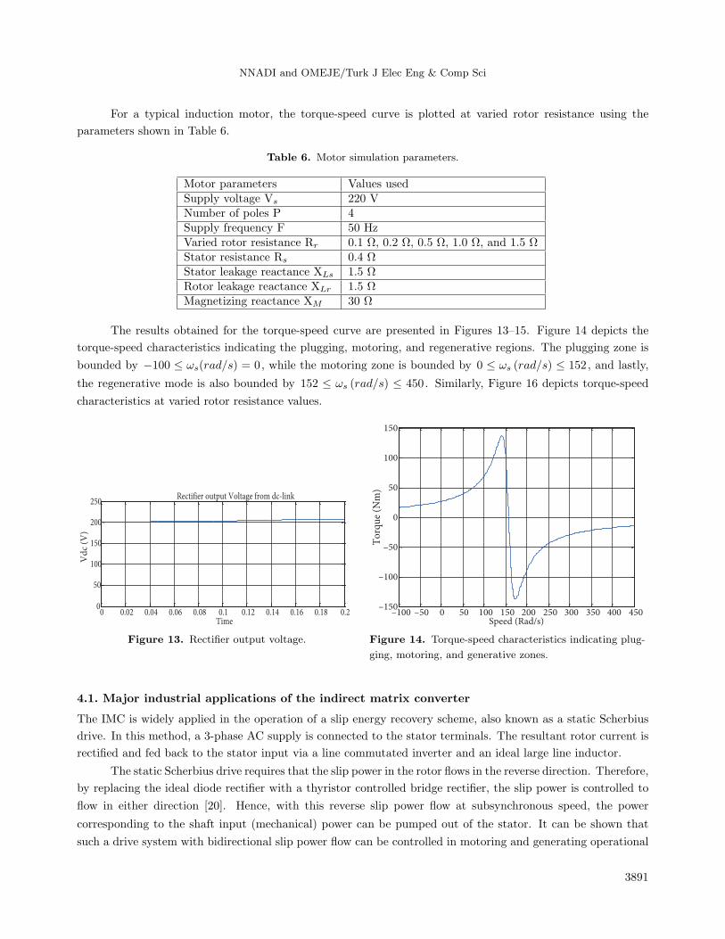
The results obtained for the torque-speed curve are presented in Figures 13–15. Figure 14 depicts the

torque-speed characteristics indicating the plugging, motoring, and regenerative regions. The plugging zone is

bounded by −100 ≤ ωs(rad/s) = 0, while the motoring zone is bounded by 0 ≤ ωs (rad/s) ≤ 152, and lastly,

the regenerative mode is also bounded by 152 ≤ ωs (rad/s) ≤ 450. Similarly, Figure 16 depicts torque-speed

characteristics at varied rotor resistance values.

0 0.02 0.04 0.06 0.08 0.1 0.12 0.14 0.16 0.18 0.20

50

100

150

200

250

Time

Rectifier output Voltage from dc-link

Vd

c (V

)

–100 –50 0 50 100 150 200 250 300 350 400 450–150

–100

–50

0

50

100

150

Speed (Rad/s)

To

rqu

e (N

m)

Figure 13. Rectifier output voltage. Figure 14. Torque-speed characteristics indicating plug-

ging, motoring, and generative zones.

4.1. Major industrial applications of the indirect matrix converter

The IMC is widely applied in the operation of a slip energy recovery scheme, also known as a static Scherbius

drive. In this method, a 3-phase AC supply is connected to the stator terminals. The resultant rotor current is

rectified and fed back to the stator input via a line commutated inverter and an ideal large line inductor.

The static Scherbius drive requires that the slip power in the rotor flows in the reverse direction. Therefore,

by replacing the ideal diode rectifier with a thyristor controlled bridge rectifier, the slip power is controlled to

flow in either direction [20]. Hence, with this reverse slip power flow at subsynchronous speed, the power

corresponding to the shaft input (mechanical) power can be pumped out of the stator. It can be shown that

such a drive system with bidirectional slip power flow can be controlled in motoring and generating operational

3891


conditions within the subsynchronous and supersynchronous speed ranges. Figure 17 presents a schematic

diagram of a slip energy recovery scheme, also called the Scherbius drive. The voltage equations for the AC

supply remains the same as those presented in Eqs. (2)–(4) above.

–2 –1.5 –1 –0.5 0 0.5 1 1.5 2–150

–100

–50

0

50

100

150

Slip

Tor

que

(N

m)

0 20 40 60 80 100 120 140 1600

50

100

150

Speed in Rad/sT

orq

ue

(Nm

)

Figure 15. A plot of torque against slip. Figure 16. A plot of torque against speed at varied rotor

resistance values.

Vb

Vc

Va

A.C SUPPLY

WOUND ROTOR

INDUCTION

MACHINE

SHAFT INPUT

POWER (1-S)Pg THREE PHASE

RECTIFIER

(IMC)

THREE PHASE

INVERTER

(PROPOSED 5 LEVEL)

THREE PHASE

TRANSFORMER

Id

L

SPg

Figure 17. Static Scherbius drive system.

If the motor runs at a given slip value “S” with the internal voltage drop neglected (ideal rotor winding),

the line to line rotor output voltage equations are represented by Eqs. (32) to (34).

VABr =Nr

Ns× S×V ml sinωrt (31)

VBCr =Nr

Ns× S×V ml sin

(ωrt−

2π

3

)(32)

3892


VCAr =Nr

Ns× S×V ml sin

(ωrt−

4π

3

)(33)

Here, Nr stands for the number of turns in the rotor windings, Ns stands for stator number of turns, and S

stands for the slip, which is the difference in synchronous speed and motor speed, all divided by the synchronous

speed value. All other variables are already known in accordance with voltage equations.

The average value of the rectifier output voltage is obtained from Eq. (35):

Vod =Np×V ml

πsin

(π

Np

)cosα (34)

Np represents the number of rectifier pulses, which in this context is 6. Vml is the rotor line to line voltage

amplitude. α is the converter control delay angle, which is always 0 for an ideal diode.

Practically, α is always taken as a second quadrant angle between 90 ≤ α ≤ 180, so that the controlled

rectifier operates in inversion mode, thereby enhancing the supply of slip power back to the AC source [20,21].

The torque developed and the rotor dissipated power are as presented in Eqs. (6)–(20) above, respectively.

A simulation was carried out to determine the dynamic and steady state performance of the wound

rotor induction machine that forms an integral part of the static Scherbius drive, as well as the rectified three

phase inverter output voltage achieved with the aid of the inductive shunt transformer. The results presented

in Figures 18–22 represent the d-q axes’ voltages and currents for the stator and rotor windings, the rotor

speed and torque produced by the machine, and the rectified inverter output voltage. Parameters used for this

simulation are presented as follows: supply voltage Vs = 200 V; stator resistance Rs = 0.4 Ω; rotor resistance

Rr = 0.2 Ω; stator and rotor leakage inductances LLs = LLr = 0.0048 H; magnetizing inductance Lm = 95.5

mH; Motor inertia J = 0.025 kgm2 ; coefficient of frictional factor B = 0.0008; N.M.S. nominal machine power

= 10 HP (7.5 kW); number of poles = 4; operating frequency = 50 Hz; synchronous speed = 1500 rpm.

0 0.01 0.02 0.03 0.04 0.05 0.06 0.07 0.08 0.09 0.1

–200

0

200

Time (s)

Vqs

(V

olt)

q–axis stator voltage in volts

0 0.01 0.02 0.03 0.04 0.05 0.06 0.07 0.08 0.09 0.1

–200

0

200

Time (s)

Vds

(V

olt)

d–axis stator voltage in volts

Figure 18. q-d axes’ stator voltage.

3893


0 0.05 0.1 0.15 0.2 0.25 0.3 0.35 0.4 0.45 0.5

–200

0

200

Time (s)

Iqr (

Amp)

q–axis rotor current in Amp

0 0.05 0.1 0.15 0.2 0.25 0.3 0.35 0.4 0.45 0.5

–200

0

200

Time (s)

Idr (

Volts

)

d–axis rotor current in Amp

Figure 19. q-d axes’ rotor current.

0 0.05 0.1 0.15 0.2 0.25 0.3 0.35 0.4 0.45 0.5–200

0

200Filtered Inverter Voltage against time

0 0.05 0.1 0.15 0.2 0.25 0.3 0.35 0.4 0.45 0.5–200

0

200

0 0.05 0.1 0.15 0.2 0.25 0.3 0.35 0.4 0.45 0.5–200

0

200

Time (s)

Van (V)

Vbn (V)

Vcn (V)

Figure 20. q-d axes’ rotor voltage.

0 0.5 1 1.50

1000

2000

3000

4000

5000

Time (s)

Roto

r–Sp

eed

(RPS

)

speed in RPS against time in s

0 0.5 1 1.5–6000

–4000

–2000

0

Time (s)

Tem

(Nm

)

Electromagnetic Torque in N.M against time in s

Figure 21. Rotor speed and torque.

3894


0 0.05 0.1 0.15 0.2 0.25 0.3 0.35 0.4 0.45 0.5–200

0

200Filtered Inverter Voltage against time

0 0.05 0.1 0.15 0.2 0.25 0.3 0.35 0.4 0.45 0.5–200

0

200

0 0.05 0.1 0.15 0.2 0.25 0.3 0.35 0.4 0.45 0.5–200

0

200

Time (s)

Van (V)

Vbn (V)

Vcn (V)

Figure 22. Three phase inverter filtered voltages.

4.2. Conclusion

Considering the motoring region of the torque slip curve of Figure 14, if the point of maximum torque is made

to intersect the torque axis, the entire motoring region is observed to be linear. This implies that the ratio of

rotor resistance to leakage reactance is set very high (R2 ≫ X2), such that the induction motor operates in

the linear region. A conventional method of obtaining higher resistance is using a conductor with a smaller

cross-sectional area or a low value diameter due to the inverse proportionality relation between resistance and

area of the conductor.

In the normal motoring region, torque is always set to a zero value when the slip of the machine is zero.

As the slip increases with a corresponding decrease in speed, torque increases in a quasilinear curve until a

breakdown or maximum torque Tmax is reached. In this region, the stator drop becomes very small with the

air gap flux remaining almost constant due to a well-adjusted value of the IMC control delay angle of Figure 5.

Beyond the breakdown torque region, Te decreases with a proportionate increase in the slip value, as shown in

Figures 14 and 15, respectively.

In the plugging region, the rotor rotates in the opposite direction to the air gap flux such that the slip

s > 1. This condition may arise if the stator supply (phase sequence) is reversed by adjusting the control delay

angle of the IMC beyond 90 when the rotor is set in motion, or due to an overhauling type of loading condition

that drives the rotor in the opposite direction. Since the torque at this condition is positive with a negative

speed value, the plugging torque appears as a breaking torque that is dissipated in the form of energy within

the machine, thus causing excessive heating of the machine.

In the regenerative region, the machine acts as a generator. The rotor moves at a supersynchronous speed

in the same direction as the air gap flux, thereby making the slip negative, thus creating a negative torque called

regenerative torque. The negative slip corresponds to the negative equivalent resistanceR

′r

S , which generates

and supplies energy back to the source, while the positive resistanceR

′r

S consumes energy during the motoring

operation.

Conclusively, the plugging region depicted in Figure 14 is bounded by −100 ≤ ωs ≤ 0rad/s , which

conforms to the negative speed value discussed earlier. The motoring region bounded by 0 ≤ ωs ≤ 152rad/s is

set within the prescribed synchronous speed value of 157.08rad/s or 1500 rpm. The regenerative mode bounded

by 152 ≤ ωs ≤ 450rad/s has a maximum speed limit greater than the synchronous speed of 157.08rad/s or 1500

3895


rpm, which also conforms to the theoretical convention thereof. Hence, for more efficient drive performance, a

three phase source of higher IMC voltage level is applied at the stator terminal to enhance an optimum drive

strategy of the above-discussed machine. The simulation result presented in Figure 21 depicts the operation

of the machine in the subsynchronous regeneration mode on attainment of a steady state condition in 0.25

s. This is because the shaft, as shown in Figure 17, is being driven by the load with the mechanical energy

converted into electrical energy, and also pumped out of the stator with a negative torque of about –1800 Nm.

The mechanical power input to the shaft Pm increases as the motor speed rises from 0 to 4000 rps between a

time interval of 0 to 0.1 s, with a corresponding decrease in slip that conforms to Eqs. (11) and (12). Under

this condition, negative power is fed to the rotor via the cycloconverter. In a time interval of 0.3 s, the motor

speed attains a steady state condition at a subsynchronous value of 950 rps, thereby raising the slip value to

0.3667. This mode of operation is typical of a variable-speed wind generation system.

The outcome of the study, in a nutshell, shows that proper voltage and frequency control was achieved

through a controlled thyristorized B2B converter. Evaluation of machine performance at varied load conditions

when driven by a well-modulated converter was achieved at reduced harmonics.

References

[1] Bueno EJ, Cobreces S, Rodriguez FJ, Hernandez A, Espinosa F. Design of a back-to-back NPC converter interface

for wind turbines with squirrel-cage induction generator. IEEE T Energy Conver 2008; 23: 932-945.

[2] Yao J, Li H, Liao Y, Chen Z. An improved control strategy of limiting the dc- link voltage fluctuation for a doubly

fed induction wind generator. IEEE T Power Electr 2008; 23: 1205-1213.

[3] Kolar JW, Friedli T, Rodriguez J, Wheeler P. Review of three-phase PWM AC-AC converter topologies. IEEE T

Ind Electron 2011; 58: 4988-5006.

[4] Zanchetta P, Wheeler P, Clare J, Bland M, Empringham L, Katsis D. Control design of a three-phase matrix-

converter-based ac-ac mobile utility power supply. IEEE T Ind Electron 2008; 55: 209-217.

[5] Bose BK. Power Electronics and AC Drives. Englewood Cliffs, NJ, USA: Prentice Hall, 2002.

[6] Friedli T, Kolar JW, Rodriguez J, Wheeler P. Comparative evaluation of three-phase AC-AC matrix converter and

voltage DC-link back-to-back converter systems. IEEE T Ind Electron 2012; 59: 4487-4510.

[7] Kumar V, Joshi RR, Bansal RC. Optimal control of matrix-converter-based WECS for performance, enhancement

and efficiency optimization. IEEE T Energy Conver 2009; 24: 264-273.

[8] Wheeler P, Rodriguez J, Clare J, Empiringham L, Weinstein A. Matrix converters: a technology review. IEEE T

Ind Electron 2002; 49: 276-288.

[9] Kolar JW, Schafmeister E, Round SD, Ertl H. Novel three-phase AC-AC sparse matrix converters. IEEE T Power

Electr 2007; 22: 1649-1661.

[10] Hojabri H, Mokhtari H, Chang L. A generalized technique of modeling, analysis and control of a matrix converter

using SVD. IEEE T Ind Electron 2011; 58: 949-959.

[11] Wei L, Lipo TA, Chan H. Matrix converter topologies with reduced number of switches. In: IEEE 2006 Power

Electronics Specialists Conference; 18-22 June 2006; Jeju, South Korea. Piscataway, NJ, USA: IEEE. pp 57-63.

[12] Liu C, Loh PC, Wang P, Blaabjerg F, Tang Y, Al-Ammar EA. Distributed generation using matrix converter in

reverse power mode. IEEE T Power Electr 2013; 28: 1072-1082.

[13] Kolar JW, Schafmeister E. Novel modulation schemes minimizing the switching losses of sparse matrix converters.

In: IEEE 2003 29th Industrial Electronics Society Conference; 2–6 November 2003; Roanoke, VA. Piscataway, NJ,

USA: IEEE. pp. 2085-2090.

3896

http://dx.doi.org/10.1109/TEC.2008.918651


http://dx.doi.org/10.1109/TIE.2011.2159353








http://dx.doi.org/10.1109/41.993260

http://dx.doi.org/10.1109/41.993260

http://dx.doi.org/10.1109/TPEL.2007.904178






http://dx.doi.org/10.1109/IECON.2003.1280564




[14] Wei L, Matsushita Y, Lipo TA. Investigation of dual-bridge matrix converters operating under unbalanced source

voltages. In: IEEE 2003 34th Power Electronic Specialists Conference; 2–6 November 2003; Roanoke VA. Piscataway,

NJ, USA: IEEE. pp. 2078-2084.

[15] Lavi A, Polge RL. Induction motor speed control with static inverter in the rotor. IEEE T Power Ap Syst 1966;

85: 76-84.

[16] Hori T, Nagase H, Hombu M. Induction motor control systems. In: Wilamowski, BM, Irwin JD, editors. Industrial

Electronics Handbook. Boca Raton, FL, USA: CRC Press, 1997. pp. 310-315.

[17] Smith GA. Static Scherbius system of induction motor speed control. IEEE T Power Electr 1977; 124: 557-565.

[18] Weiss HW. Adjustable speed AC drive systems for pump and compressor applications. IEEE T Ind Appl 1974; 10:

157-162.

[19] Fitzgerald AE. Electric Machinery. 5th ed. New York, USA: McGraw-Hill, 1990.

[20] Pena R, Clare JC, Asher GM. Doubly fed induction generator using back-to-back PWM converters and its appli-

cation to variable speed wind energy generation. IEE P-Elect Pow Appl 1996; 143: 234-240.

[21] Barnes M, Dimeas A, Engler A, Fitzer C, Hatziargyriou N, Jones C, Papathanassiou S, Vandenbergh M. Microgrid

laboratory facilities. In: International Conference on Future Power Systems; 16–18 November 2005; Amsterdam,

the Netherlands. Piscataway, NJ, USA: IEEE. pp. 1-6.

3897

http://dx.doi.org/10.1109/PESC.2003.1216775



http://dx.doi.org/10.1109/FPS.2005.204229



steady state analysis of a three phase indirect matrix...

Documents