steam generator efficiency by forecasting production ...stmlportal.net/ictom04/papers/p43.pdf ·...

ICTOM 04 – 4th International Conference on Technology and Operations Management

447

STEAM GENERATOR EFFICIENCY BY FORECASTING

PRODUCTION METHOD

CASE STUDY AT PT. CVX IN INDONESIA

Yudi Suherdi,

School of Business and Management-ITB,

J1. Ganesha 10 Bandung 40132, Indonesia.

Email: [email protected]@yahoo.com

Central Steam Station Area 5 PTCVX Indonesia

ABSTRACT

Steam Supply Team, under Facility Operation - Heavy Oil Department, PTCVX. Base on decreasing

demand steam supply injector, due to cause by many saturated reservoir (mature).Will be impact to

reducing number of steam generator.

The purpose of this research is to find out the quantitative research by forecasting production method,

plant size, and maintenance cost steam generator consideration, will be affect maintenance cost.

The method in this research is taking secondary data of steam production in 2011, up to 2013 and result

production forecast can be count production capacity, and this research is to final out steam generator

availability meet with steam distribution injector and formation demand.

This research used compare steam maintenance cost before efficiency analysis, with steam maintenance

cost after efficiency analysis, to know correlation production forecast with steam generator availability,

known as plant size.

The result of this research is concluded that the proper model to production forecast and maintenance cost

consideration will be significant affect to steam generator efficiency level at Central Steam Station area 5

PT CVX, and suitability steam generator availability with steam supply demand is influent factor

Key words: Production Forecast, Plant Size, Total Steam Generator, Maintenance Cost, Efficiency

Steam Generator

1. Introduction

Until now, oil is the largest energy resource and the most widely used in Indonesia and in the world. The

development of technology and industry in Indonesia is in separable from the role of oil as a source of

energy. Therefore, Indonesia as one of the largest oil producing countries in the world need an expert to

be able to explore and extract oil from the wells, and then process them into valuable products

economically and efficiently

Method of increasing oil production is carried out in the Duri field using the injection of steam (steam

flooding). Steam flooding is a method for reducing the viscosity of heavy oil. The heat from the steam

injection reduces the viscosity of the oil when the oil from pushing steam injector wells to the production

wells. Steam flooding is an improved method of acquisition (secondary recovery).To meet the demand for

steam heat, it can take a steam generator system. Steam generator utilizes three types of heat transfer to

convert water into steam that is; conduction, convection and radiation. The resulting steam will be

injected into the well injection.

In general there aretwotypesof steamgeneratorsinthe CVX, namely:

a. Type 50 MMBTU/H, typically used for steam flood applications. This type can produce 3.500

barrels of steam per day with80% quality steam.

b. Types 25 and 22 MMBTU/H, but can be used for steam flood, used also for cyclic operation due

to size considerations. These types can produce720 barrels of steam per day with 70% quality

steam.

mailto:[email protected]

mailto:[email protected]


448

FigureI.1. Steam Generator

Source: Operation and Maintenance Certification Steam generator

The working principles of the steam generator are:

1. The water comes from a water treating plant (WTP) with a temperature of 160°F, pumped wore

the feed water pump (FWP) to the pre-heater (pressure1225 psi)

2. At the pre-heated water heater (heat exchanger system; into approximately 220°F) using already

hot water coming out of the convection section

3. Subsequent water flow in to the convection section and toward the radiant section passing

through the pre-heater. In the convection section, water gets hotter than the rest of the exhaust gas

(water temperature of approximately 540°F). In pre-heater temperature down to around 450°F,

because it is absorbed by the heat exchanger.

4. On the radiant section, the water is heated using a burner combustion products that turn in to

vapor (temperature around 505-520°F, Pressure 800Psi, 73% quality steam)

5. Steam then flows through a steam injection wells to the distribution line

Feed water from the water treatment plant in soft water will be pumped by Feed Water Pump with a

pressure of 1,200 PSI to the pre-heater. Water temperature is180ºFsoft ware is then heated using a pre-

heater called Double Pipe Heat Exchanger. This soft water temperature increases be220ºF. Heating

medium used by the heat exchangers water that has been experienced in the area ofconvection heating.

The illustration below shows the direction of flow that occurs in a pre-heater. Preheating is intended to

prevent the formation of acid from SO2 and SO3compounds contained in the fuel and will form a crust

(scale) which is corrosive to pipes convection chamber. Then the soft water will flow into the convection region. In the area of soft water will be heated to a

temperature of vapor. Heating medium used in this area comes from the combustion gases of the burner.

Water that has been through this process will increase the temperature to 450º-540ºF. In this section, the

water also decreased pressure (pressure drop) to 960 PSI so that when leaving the convection chamber,

some steam has been formed. Steam generated from this section has the quality to 50%.

After passing the initial heater (pre heater), the water will go to space radiation from the generator. In this

space, the water absorbs heat from the burner flame produced by the burner (burner). Water that has been

through this area will turn into steam temperature is 500ºF with 1100 PSI of pressure. The resulting steam

has a quality between 73% -80%. Furthermore, the entire steam generated in the steam header will be

collected and supplied to the injector well. To see the processing of the steam generator to be seen P&ID (piping and instrumentation diagram) as

shown below as follows:


449

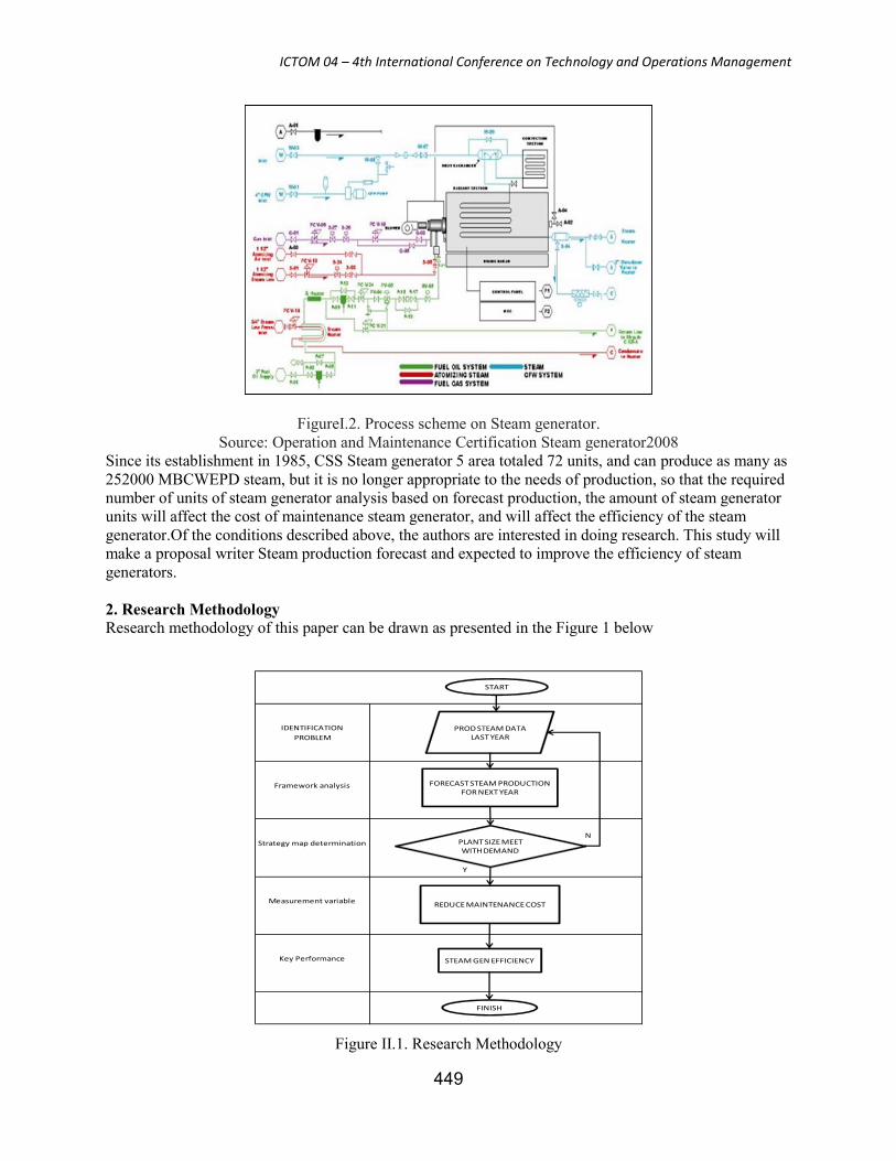
FigureI.2. Process scheme on Steam generator.

Source: Operation and Maintenance Certification Steam generator2008

Since its establishment in 1985, CSS Steam generator 5 area totaled 72 units, and can produce as many as

252000 MBCWEPD steam, but it is no longer appropriate to the needs of production, so that the required

number of units of steam generator analysis based on forecast production, the amount of steam generator

units will affect the cost of maintenance steam generator, and will affect the efficiency of the steam

generator.Of the conditions described above, the authors are interested in doing research. This study will

make a proposal writer Steam production forecast and expected to improve the efficiency of steam

generators.

2. Research Methodology

Research methodology of this paper can be drawn as presented in the Figure 1 below

IDENTIFICATION

PROBLEM

Framework analysis

Strategy map determination

Measurement variable

Key Performance

FORECAST STEAM PRODUCTION FOR NEXT YEAR

START

PROD STEAM DATA LAST YEAR

PLANT SIZE MEET WITH DEMAND

REDUCE MAINTENANCE COST

STEAM GEN EFFICIENCY

FINISH

N

Y

Figure II.1. Research Methodology


450

Analysis of forecast methods that will be used from this study is to compare the forecast production of

steam generators, the Moving Average method, Weighing Moving Average, and Exponential Smoothing,

so that researchers will be easier to determine a more precise forecast method to be used.

Analysis of the data of this study is to compare the cost of production of steam generators prior to

analysis forecast, the cost of production of steam generators after analysis forecast.

To ascertain the correlation between the numbers of units of steam generator which is operated by the

amount of steam generators operating costs, the software will be demonstrated using scatter plots

To be able to know the amount of steam produced is, of course, requires forecasting future production

based on data taken last period. The usefulness of such forecasting is to establish policies relating to the

determination of the required amount of steam generator.

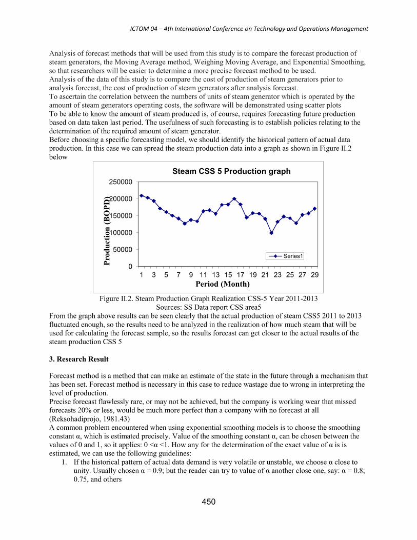
Before choosing a specific forecasting model, we should identify the historical pattern of actual data

production. In this case we can spread the steam production data into a graph as shown in Figure II.2

below

Figure II.2. Steam Production Graph Realization CSS-5 Year 2011-2013

Sources: SS Data report CSS area5

From the graph above results can be seen clearly that the actual production of steam CSS5 2011 to 2013

fluctuated enough, so the results need to be analyzed in the realization of how much steam that will be

used for calculating the forecast sample, so the results forecast can get closer to the actual results of the

steam production CSS 5

3. Research Result

Forecast method is a method that can make an estimate of the state in the future through a mechanism that

has been set. Forecast method is necessary in this case to reduce wastage due to wrong in interpreting the

level of production.

Precise forecast flawlessly rare, or may not be achieved, but the company is working wear that missed

forecasts 20% or less, would be much more perfect than a company with no forecast at all

(Reksohadiprojo, 1981.43)

A common problem encountered when using exponential smoothing models is to choose the smoothing

constant α, which is estimated precisely. Value of the smoothing constant α, can be chosen between the

values of 0 and 1, so it applies: 0 <α <1. How any for the determination of the exact value of α is is

estimated, we can use the following guidelines:

1. If the historical pattern of actual data demand is very volatile or unstable, we choose α close to

unity. Usually chosen α = 0.9; but the reader can try to value of α another close one, say: α = 0.8;

0.75, and others

0

50000

100000

150000

200000

250000

1 3 5 7 9 11 13 15 17 19 21 23 25 27 29

Pro

du

ctio

n (

BO

PD

)

Period (Month)

Steam CSS 5 Production graph

Series1


451

2. If the historical pattern of actual data request does not fluctuate or relatively stable, we chose α is

close to zero. Usually chosen value α = 0.1, but the reader can try to value of α another is close to

zero, say: α = 0.1; 0.2; 0.3, and etc

Based on the intensive analysis of company’s nature of business and if the historical pattern of actual data

production is highly volatile or unstable over time, it can be chosen value of α is close to one. Usually

chosen value α = 0.9; 0.8; 0.75 and in this study used the value α = 0.8, as it would lead to a value of one.

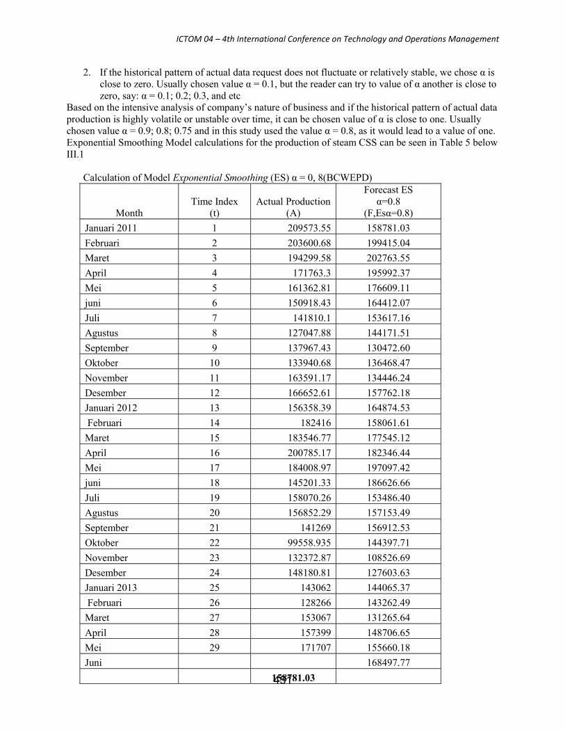
Exponential Smoothing Model calculations for the production of steam CSS can be seen in Table 5 below

III.1

Calculation of Model Exponential Smoothing (ES) α = 0, 8(BCWEPD)

Month

Time Index

(t)

Actual Production

(A)

Forecast ES

α=0.8

(F,Esα=0.8)

Januari 2011 1 209573.55 158781.03

Februari 2 203600.68 199415.04

Maret 3 194299.58 202763.55

April 4 171763.3 195992.37

Mei 5 161362.81 176609.11

juni 6 150918.43 164412.07

Juli 7 141810.1 153617.16

Agustus 8 127047.88 144171.51

September 9 137967.43 130472.60

Oktober 10 133940.68 136468.47

November 11 163591.17 134446.24

Desember 12 166652.61 157762.18

Januari 2012 13 156358.39 164874.53

Februari 14 182416 158061.61

Maret 15 183546.77 177545.12

April 16 200785.17 182346.44

Mei 17 184008.97 197097.42

juni 18 145201.33 186626.66

Juli 19 158070.26 153486.40

Agustus 20 156852.29 157153.49

September 21 141269 156912.53

Oktober 22 99558.935 144397.71

November 23 132372.87 108526.69

Desember 24 148180.81 127603.63

Januari 2013 25 143062 144065.37

Februari 26 128266 143262.49

Maret 27 153067 131265.64

April 28 157399 148706.65

Mei 29 171707 155660.18

Juni 168497.77

158781.03


452

Table above column 4 calculation using the equation;

Ft = Ft-1 + α( At-1 – Ft-1 )

When : Ft = forecast value for a period of time to - t

Ft-1 = forecast value for the previous period, t-1

At-1 = Actual value for the previous period, t-1

α = Smoothing constan

Note: For the first month of the forecast can be done by taking the average of the observed data.

If : Ft-1 = 158781

At-1 = 209573.5

α = 0,8

( For Februari ) Ft = 158781 + 0,8 ( 209573.5 – 158781 )

= 158781 + 0,8 ( 50792.5 )

= 158781 + ( 40634 )

= 199415

( For March ) Ft = 199415 + 0,8 ( 203600.6 – 199415 )

= 199415 + 0,8 ( 4185.6 )

= 497,72 + (3348.4 )

= 202763.5 and next step

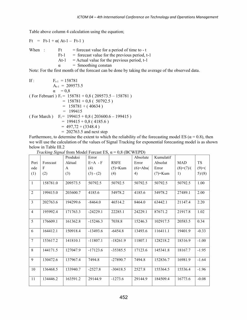
Furthermore, to determine the extent to which the reliability of the forecasting model ES (α = 0.8), then

we will use the calculation of the values of Signal Tracking for exponential forecasting model is as shown

below in Table III.2

Tracking Signal from Model Forcast ES, α = 0,8 (BCWEPD)

Peri

ode

(1)

Forecast

F

(2)

Produksi

Aktual

A

(3)

Error

E=A - F

(4)

(3) - (2)

RSFE

(5)=Kum

(4)

Absolute

Error

(6)=Abs(

4)

Kumulatif

Absolut

Error

(7)=Kum

MAD

(8)=(7)/(

1)

TS

(9)=(

5)/(8)

1 158781.0 209573.5 50792.5 50792.5 50792.5 50792.5 50792.5 1.00

2 199415.0 203600.7 4185.6 54978.2 4185.6 54978.2 27489.1 2.00

3 202763.6 194299.6 -8464.0 46514.2 8464.0 63442.1 21147.4 2.20

4 195992.4 171763.3 -24229.1 22285.1 24229.1 87671.2 21917.8 1.02

5 176609.1 161362.8 -15246.3 7038.8 15246.3 102917.5 20583.5 0.34

6 164412.1 150918.4 -13493.6 -6454.8 13493.6 116411.1 19401.9 -0.33

7 153617.2 141810.1 -11807.1 -18261.9 11807.1 128218.2 18316.9 -1.00

8 144171.5 127047.9 -17123.6 -35385.5 17123.6 145341.8 18167.7 -1.95

9 130472.6 137967.4 7494.8 -27890.7 7494.8 152836.7 16981.9 -1.64

10 136468.5 133940.7 -2527.8 -30418.5 2527.8 155364.5 15536.4 -1.96

11 134446.2 163591.2 29144.9 -1273.6 29144.9 184509.4 16773.6 -0.08


453

12 157762.2 166652.6 8890.4 7616.9 8890.4 193399.8 16116.7 0.47

13 164874.5 156358.4 -8516.1 -899.3 8516.1 201916.0 15532.0 -0.06

14 158061.6 182416.0 24354.4 23455.1 24354.4 226270.3 16162.2 1.45

15 177545.1 183546.8 6001.7 29456.8 6001.7 232272.0 15484.8 1.90

16 182346.4 200785.2 18438.7 47895.5 18438.7 250710.7 15669.4 3.06

17 197097.4 184009.0 -13088.5 34807.0 13088.5 263799.2 15517.6 2.24

18 186626.7 145201.3 -41425.3 -6618.3 41425.3 305224.5 16956.9 -0.39

19 153486.4 158070.3 4583.9 -2034.4 4583.9 309808.4 16305.7 -0.12

20 157153.5 156852.3 -301.2 -2335.6 301.2 310109.6 15505.5 -0.15

21 156912.5 141269.0 -15643.5 -17979.2 15643.5 325753.1 15512.1 -1.16

22 144397.7 99558.9 -44838.8 -62817.9 44838.8 370591.9 16845.1 -3.73

23 108526.7 132372.9 23846.2 -38971.7 23846.2 394438.0 17149.5 -2.27

24 127603.6 148180.8 20577.2 -18394.6 20577.2 415015.2 17292.3 -1.06

25 144065.37 143061.8 -1003.60 -19398.17 1003.60 416018.80 16640.75 -1.17

26 143262.49 128266.4 -14996.07 -34394.23 14996.07 431014.87 16577.49 -2.07

27 131265.64 153066.9 21801.26 -12592.97 21801.26 452816.13 16770.97 -0.75

28 148706.65 157398.6 8691.92 -3901.06 8691.92 461508.05 16482.43 -0.24

29 155660.18 171707.2 16046.98 12145.92 16046.98 477555.02 16467.41 0.74

Source: Result Data Processing in 2013

Table above column 4 calculation using the equation;

Calculation of Signal Tracking Forecasting Model ES, α = 0.8 (BCWEPD)

Formula: Error Forecast = Xt - Ft

(For column 4)

Period 1 Error: 209573.5 - 158 781 = 50792.5

Period 2 Error: 203600.6 - 199 415 = 4185.6

Period 3 Error: 194299.5 - 202763.5 = -8463.9 and next step

(For column 5 is cumulative from column 4)

Period 2 50792.5 + 4185.6 = 54978.1

Period 3 54978.1 + -8463.9 = 46514.1

Period 4 46514.1 + -24229 = 22285.1 and next step

(For column 6)

The formula:

AE │ Xt - Ft │

(Period 1) Absolute Error MA4 = 209573.5 - 158 781 = 50792.5

(Period 2) Absolute Error MA4 = 203600.6 - 199 415 = 4185.6


454

(Period 3) Absolute Error MA4 = 194299.5 - 202763.5 = 8463.9

(Period 4) Absolute Error MA4 = 171763.3 - 195992.3 = 24229

(For column 7 is cumulative from column 6)

Period 2 50792.5 + 4185.6 = 54978.1

Period 3 54978.1 + 8463.9 = 63442.1

Period 4 63442.1 + 24229 = 87671.1 and next step

(For column 8)

The formula:

∑ (Absolute dari forecast errors)

nMAD =

Period 2 54978.1 / 2 = 27489

Period 3 63442.1 / 3 = 21147.3

Period 4 87671.1 / 4 = 21917.7 and next step.

(For column 9)

The formula:

Tracking Signal =

Period 2 54978.1 / 27489 = 2

Period 3 46514.1 / 21147.3 = 2.1

Period 4 22285.1 / 21917.7 = 1 and next step.

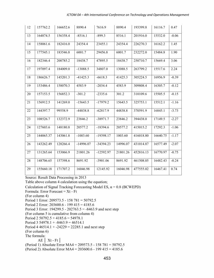
From Table III.2 above shows that the value - the value of Signal Tracking for exponential smoothing

models, ES (α = 0.8) are within limits that can be accepted (maximum of ± 4), where the values of the

Signal Tracking moves - 3.73 to +3.06. And can map as figure below;

Figure III.1. Map Tracking Control of Model E Signal Smoothing

Sources: Data Processing Results in 2013

The picture above shows that the accuracy of forecasting models ES (α = 0.8) can be relied upon

Because it is within limits Signal Tracking control. A good Signal Tracking has RSFE low and has a lot

of positive same error with a negative error, so the Signal Tracking center close to zero. It has been able

to be met by the ES forecasting model (α = 0.8), so that the forecasting model can be selected as an

appropriate model to describe the pattern of production of steam CSS 5.

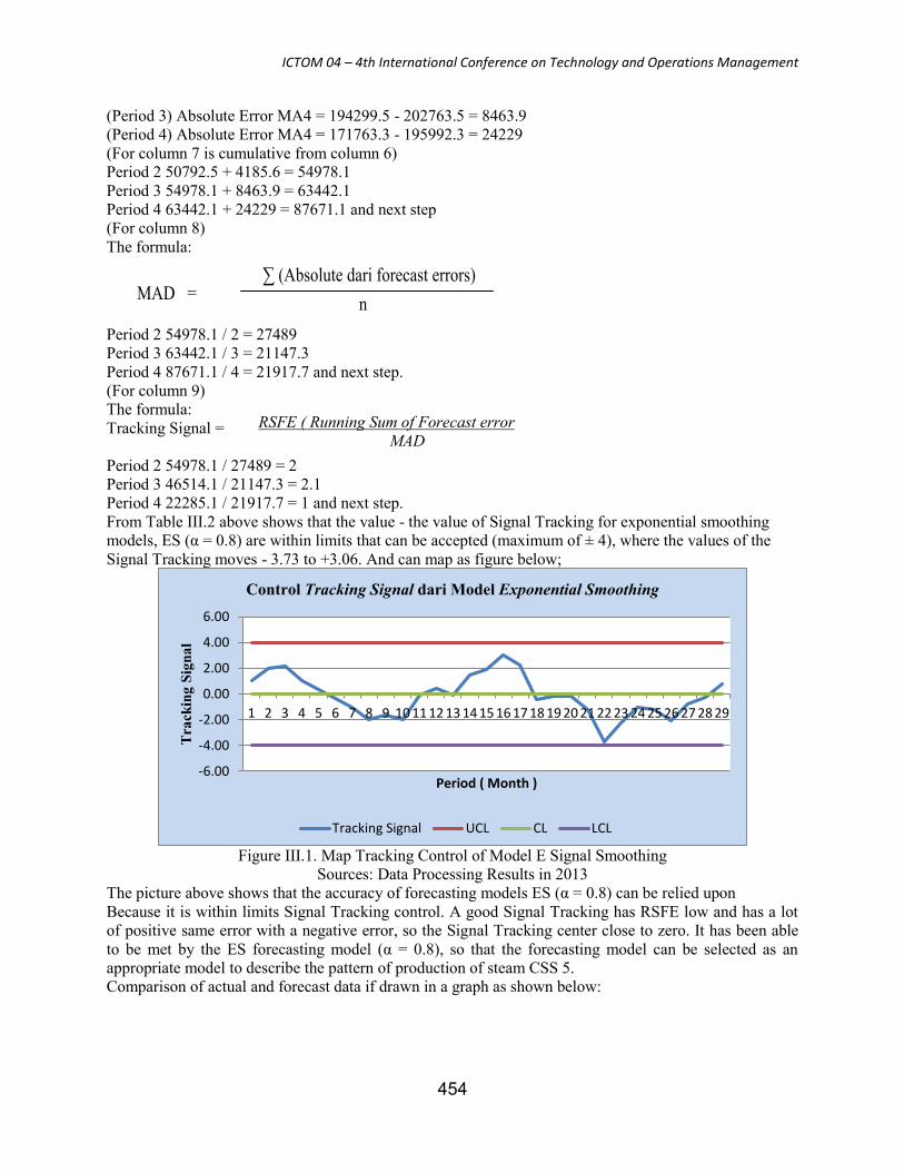
Comparison of actual and forecast data if drawn in a graph as shown below:

-6.00

-4.00

-2.00

0.00

2.00

4.00

6.00

1 2 3 4 5 6 7 8 9 10 11 12 13 14 15 16 17 18 19 20 21 22 23 24 25 26 27 28 29

Tra

ckin

g S

ign

al

Period ( Month )

Control Tracking Signal dari Model Exponential Smoothing

Tracking Signal UCL CL LCL

RSFE ( Running Sum of Forecast error

MAD


455

Figure III.2. Comparison of Actual and Forecast Steam in 2013

Sources: Data processing 2013

From the graph above results can be seen clearly that the forecast result is different from the actual red-

colored red production, so that the analysis can be obtained from the results of the steam generator unit

capacity according to customer requirements.

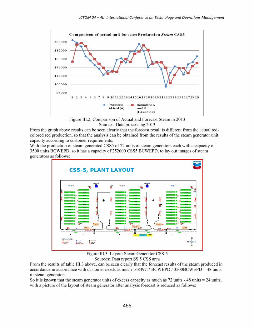
With the production of steam generated CSS5 of 72 units of steam generators each with a capacity of

3500 units BCWEPD, so it has a capacity of 252000 CSS5 BCWEPD, to lay out images of steam

generators as follows:

Figure III.3. Layout Steam Generator CSS-5

Sources: Data report SS 5 CSS area

From the results of table III.3 above, can be seen clearly that the forecast results of the steam produced in

accordance in accordance with customer needs as much 168497.7 BCWEPD / 3500BCWEPD = 48 units

of steam generator.

So it is known that the steam generator units of excess capacity as much as 72 units - 48 units = 24 units,

with a picture of the layout of steam generator after analysis forecast is reduced as follows:


456

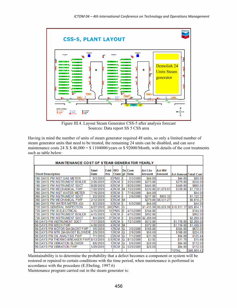
Figure III.4. Layout Steam Generator CSS-5 after analysis forecast

Sources: Data report SS 5 CSS area

Having in mind the number of units of steam generator required 48 units, so only a limited number of

steam generator units that need to be treated, the remaining 24 units can be disabled, and can save

maintenance costs 24 X $ 46,000 = $ 1104000/years or $ 92000/Month, with details of the cost treatments

such as table below:

Maintainability is to determine the probability that a defect becomes a component or system will be

restored or repaired to certain conditions with the time period, when maintenance is performed in

accordance with the procedure (E.Ebeling, 1997.6)

Maintenance program carried out in the steam generator is:

Demolish 24

Units Steam

generator


457

a. PM (preventive maintenance) is a treatment program that is done to shut down due to the prevention of

unplanned damage (unplanned shut down), and includes the replacement of parts that are already planned

1. 90 Days PM Boiler

2. 180 Days PM Instrument Boiler

3. 360 Days PM Boiler

4. 720 Days PM Mechanical FWP

5. 720 Days General Inspection

6. 180 Days PM Instrument SDCT

7. 360 Days PM Instrument Water Meter

8. 180 Days PM Instrument Gas Meter

b. PdM (predictive maintenance) is a treatment program that is done to shut down due to the prevention of

unplanned damage (unplanned shut down), but not including parts replacement, only performance data

collection equipment, such as vibration of data, the data thermograph, and the data turbology

1. 90 Days PM Vibration FWP

2. 90 Days PM Vibration Blower

3. 90 Days PM Thermograph Breaker FWP

4. 90 Days PM Thermograph MCC

5. 90 Days PM Oil Analysis FWP

Production costs in the long run can add all the factors of production or inputs used her, all kinds of costs

incurred is the cost of change, including labor costs, maintenance costs, and the cost of other production

equipment.

In the long term the company should determine the amount of capacity of the plant (plant size) that will

minimize the cost of production (Sukirno, 2003.214)

In the economic analysis of plant capacity curve described by the average total cost (average cost). Thus

analyzes manufacturers in their efforts to analyze production activities minimize costs.Care costs will

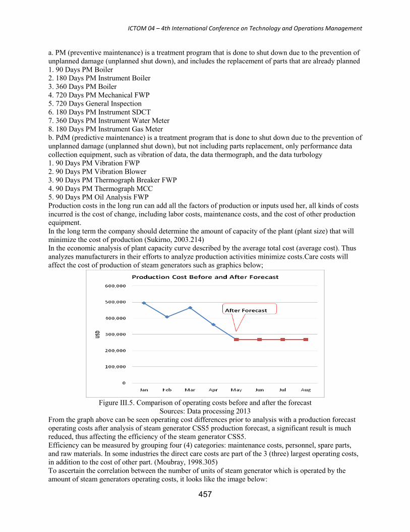
affect the cost of production of steam generators such as graphics below;

Figure III.5. Comparison of operating costs before and after the forecast


From the graph above can be seen operating cost differences prior to analysis with a production forecast

operating costs after analysis of steam generator CSS5 production forecast, a significant result is much

reduced, thus affecting the efficiency of the steam generator CSS5.

Efficiency can be measured by grouping four (4) categories: maintenance costs, personnel, spare parts,

and raw materials. In some industries the direct care costs are part of the 3 (three) largest operating costs,

in addition to the cost of other part. (Moubray, 1998.305)

To ascertain the correlation between the number of units of steam generator which is operated by the

amount of steam generators operating costs, it looks like the image below:


458

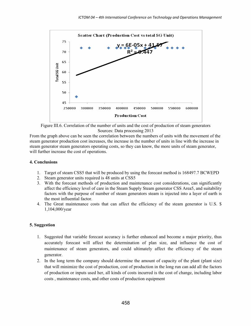
Figure III.6. Correlation of the number of units and the cost of production of steam generators


From the graph above can be seen the correlation between the numbers of units with the movement of the

steam generator production cost increases, the increase in the number of units in line with the increase in

steam generator steam generators operating costs, so they can know, the more units of steam generator,

will further increase the cost of operations.

4. Conclusions

1. Target of steam CSS5 that will be produced by using the forecast method is 168497.7 BCWEPD

2. Steam generator units required is 48 units at CSS5

3. With the forecast methods of production and maintenance cost considerations, can significantly

affect the efficiency level of care in the Steam Supply Steam generator CSS Area5, and suitability

factors with the purpose of number of steam generators steam is injected into a layer of earth is

the most influential factor.

4. The Great maintenance costs that can affect the efficiency of the steam generator is U.S. $

1,104,000/year

5. Suggestion

1. Suggested that variable forecast accuracy is further enhanced and become a major priority, thus

accurately forecast will affect the determination of plan size, and influence the cost of

maintenance of steam generators, and could ultimately affect the efficiency of the steam

generator.

2. In the long term the company should determine the amount of capacity of the plant (plant size)

that will minimize the cost of production, cost of production in the long run can add all the factors

of production or inputs used her, all kinds of costs incurred is the cost of change, including labor

costs , maintenance costs, and other costs of production equipment


459

3. Efficiency can be measured by four (4) categories: maintenance costs, personnel, parts, and raw

material. In some industries the direct care costs are part of the 3 (three) largest operating costs, in

addition to the cost of other raw material.

6. References

1. Anonim.2008.Operation and Maintenance Certification Steam Generator.Duri : O&MC – HR

Learning and Development PT.CPI

2. Charles E.Ebeling.Reability and Maintainability Engineering, Universityof Dayton, 1997.

3. Ginting,Rosnani,system Produksi,Graha Ilmu, Yogyakarta, 2007.

4. John Moubray, Reliability CenteredMaintenance, Linacre house Oxford, 1998.

5. Makridakis, Spyros, Forecasting Metods dan Application,John Wiley, United State of America,

1998.

6. Michael L.George, Lean Six Sigma Pocket, McGraw-Hill, New York, 2005

7. Sadono Sukirno,Pengantar Teori Mikroekonomi.Jakarta :PT RajaGrafindo Persada, 2003

8. HTTP:// www.chevron.com. Access on 25 June 2014

steam generator efficiency by forecasting production ...stmlportal.net/ictom04/papers/p43.pdf ·...

Documents