steep creek assessment methodology - rdck
TRANSCRIPT

BGC ENGINEERING INC. 500-980 Howe Street, Vancouver, BC Canada V6Z 0C8 Tel: 604.684.5900 Fax: 604.684.5909
RDCK FLOODPLAIN AND STEEP CREEK STUDY
Steep Creek Assessment Methodology
FINAL March 31, 2020
BGC Project No.: 0268007
BGC Document No.: RDCK2-SC-011F
Prepared by BGC Engineering Inc. for: Regional District of Central Kootenay

Regional District of Central Kootenay March 31, 2020 RDCK Floodplain and Steep Creek Study, Steep Creek Assessment Methodology Project No.: 0268007
BGC ENGINEERING INC. ii
TABLE OF REVISIONS
DRAFT February 11, 2020 Original issue
FINAL March 31, 2020 Final issue
LIMITATIONS BGC Engineering Inc. (BGC) prepared this document for the account of Regional District of Central Kootenay. The material in it reflects the judgment of BGC staff in light of the information available to BGC at the time of document preparation. Any use which a third party makes of this document or any reliance on decisions to be based on it is the responsibility of such third parties. BGC accepts no responsibility for damages, if any, suffered by any third party as a result of decisions made or actions based on this document.
As a mutual protection to our client, the public, and ourselves, all documents and drawings are submitted for the confidential information of our client for a specific project. Authorization for any use and/or publication of this document or any data, statements, conclusions or abstracts from or regarding our documents and drawings, through any form of print or electronic media, including without limitation, posting or reproduction of same on any website, is reserved pending BGC’s written approval. A record copy of this document is on file at BGC. That copy takes precedence over any other copy or reproduction of this document.

Regional District of Central Kootenay March 31, 2020 RDCK Floodplain and Steep Creek Study, Steep Creek Assessment Methodology Project No.: 0268007
BGC ENGINEERING INC. iii
TABLE OF CONTENTS TABLE OF REVISIONS ........................................................................................................... ii LIMITATIONS ........................................................................................................................... ii LIST OF TABLES .................................................................................................................... vi LIST OF FIGURES ................................................................................................................. vii 1. STEEP CREEK PROCESS TYPES ............................................................................. 1 1.1. Steep Creek Watersheds and Fans ........................................................................... 2 1.2. Debris Flows ................................................................................................................ 7 1.3. Debris Floods .............................................................................................................. 9 1.4. Clear-water Floods on Alluvial Fans ....................................................................... 13 2. STEEP CREEK HAZARD ASSESSMENT METHODS FOR DEBRIS-FLOOD PRONE
CREEKS ..................................................................................................................... 15 2.1. Introduction ............................................................................................................... 15 2.2. Hazard Assessment Methods Background ............................................................ 15 2.2.1. Frequency-Magnitude Relationships ........................................................................ 15 2.2.2. Return Period Classes .............................................................................................. 16 2.3. Hazard Assessment Workflow ................................................................................. 17 2.4. Basis for Hazard Process Characterization ............................................................ 19 2.4.1. Desktop Study .......................................................................................................... 19 2.4.1.1. Historical Records Review ...................................................................................... 19 2.4.1.2. Air Photo Review .................................................................................................... 19 2.4.1.3. LiDAR Review ........................................................................................................ 20 2.4.2. Field Investigation ..................................................................................................... 20 2.4.2.1. Field Mapping ......................................................................................................... 20 2.4.2.2. Test Trenching and Radiocarbon Dating ................................................................ 21 2.4.2.3. Dendrogeomorphology ........................................................................................... 21 2.4.2.4. Bed Material Sampling ........................................................................................... 23 2.5. Hazard Process Characterization ............................................................................ 24 2.5.1. Process Characterization .......................................................................................... 24 2.5.1.1. Drainage Basin ....................................................................................................... 24 2.5.1.2. Stream Channel ...................................................................................................... 25 2.5.1.3. Deposits .................................................................................................................. 25 2.5.2. Flood & Debris Flood Frequency-Discharge Relationship ........................................ 30 2.5.2.1. Clearwater Peak Flow Estimation ........................................................................... 30 2.5.2.2. Discharge Bulking Method ...................................................................................... 31 2.5.3. Debris Flood Frequency-Volume Relationship ......................................................... 36 2.5.3.1. Regional Debris Flood Frequency-Volume Relationship ........................................ 37 2.5.3.2. Empirical Area-Volume Relationship ...................................................................... 39 2.5.3.3. Sediment Transport Relationship ........................................................................... 39 2.5.3.4. Comparison with Regional Debris Flood Frequency-Volume ................................. 41 2.6. Spatial Hazard Characterization .............................................................................. 42 2.6.1. Bank Erosion ............................................................................................................ 42 2.6.1.1. Air Photo Calibration ............................................................................................... 42 2.6.1.2. Modelling Approach ................................................................................................ 43

Regional District of Central Kootenay March 31, 2020 RDCK Floodplain and Steep Creek Study, Steep Creek Assessment Methodology Project No.: 0268007
BGC ENGINEERING INC. iv
2.6.1.3. Interpretation of Results ......................................................................................... 44 2.6.2. Debris-Flood Assessment – Hydrodynamic Modelling and Mapping ........................ 45 2.6.2.1. Introduction ............................................................................................................. 45 2.6.2.2. HEC-RAS 2D Modelling Development ................................................................... 46 2.6.2.3. FLO-2D Modelling Development ............................................................................ 49 2.6.3. Principles of Modelling Scenario Definition ............................................................... 52 2.6.3.1. Background ............................................................................................................ 52 2.6.3.2. Blockage Scenarios ................................................................................................ 52 2.6.3.3. Dike Breach Scenarios ........................................................................................... 54 2.7. Hazard Mapping ........................................................................................................ 55 2.7.1. Introduction ............................................................................................................... 55 2.7.2. Hazard Intensity Mapping ......................................................................................... 56 2.7.3. Interpreted Hazard Maps and Composite Hazard Maps ........................................... 56 2.8. Error and Uncertainty ............................................................................................... 61 2.8.1. Regional Flood Frequency Analysis ......................................................................... 62 2.8.2. Debris Flood Frequency-Volume Analysis ................................................................ 62 2.8.3. Debris Flood Frequency-Peak Discharge Analysis ................................................... 63 2.8.4. Bank Erosion Analysis .............................................................................................. 63 2.8.4.1. Air Photo Assessment ............................................................................................ 63 2.8.4.2. Bank Erosion Predictions ....................................................................................... 64 2.8.5. Numerical Runout Modelling Uncertainty .................................................................. 65 2.8.5.1. HEC RAS ................................................................................................................ 66 2.8.5.2. FLO 2D ................................................................................................................... 66 2.8.6. Hazard Mapping ....................................................................................................... 66 2.8.7. Uncertainty Summary ............................................................................................... 67 3. REGIONAL FLOOD FREQUENCY ANALYSIS METHODS ...................................... 69 3.1. Introduction ............................................................................................................... 69 3.1.1. Regional FFA ............................................................................................................ 69 3.1.2. Index-flood Method ................................................................................................... 69 3.1.3. Application to Ungauged Watersheds....................................................................... 70 3.2. Study Area ................................................................................................................. 70 3.3. Data Acquisition and Compilation ........................................................................... 72 3.3.1. Hydrometric Stations................................................................................................. 72 3.3.2. Flood Records .......................................................................................................... 72 3.3.3. Maximum Peak Instantaneous Discharge ................................................................ 72 3.3.4. Watershed Polygons ................................................................................................. 73 3.3.5. Watershed Areas ...................................................................................................... 73 3.3.6. Watershed Characteristics ........................................................................................ 74 3.3.6.1. Watershed Statistics ............................................................................................... 74 3.3.6.2. Climate Variables ................................................................................................... 74 3.3.6.3. Land cover .............................................................................................................. 75 3.3.6.4. Curve Number ........................................................................................................ 75 3.4. Methods and Assumptions ...................................................................................... 78 3.4.1. Flood Statistics Calculations ..................................................................................... 78 3.4.1.1. L-moments .............................................................................................................. 78 3.4.1.2. At-site Peak Discharge Estimates .......................................................................... 79 3.4.2. Formation of Hydrological Regions ........................................................................... 80 3.4.2.1. Data Preparation .................................................................................................... 80 3.4.2.2. Number of Hydrological Regions ............................................................................ 80

Regional District of Central Kootenay March 31, 2020 RDCK Floodplain and Steep Creek Study, Steep Creek Assessment Methodology Project No.: 0268007
BGC ENGINEERING INC. v
3.4.2.3. Manual Adjustments of Hydrologic Regions ........................................................... 81 3.4.2.4. Refinement of the Hydrometric Station Selection ................................................... 81 3.4.2.5. Testing for Homogeneity ........................................................................................ 82 3.4.3. Regionalization ......................................................................................................... 82 3.4.3.1. Regional L-moments .............................................................................................. 82 3.4.3.2. Distribution Selection for Growth Curves ................................................................ 83 3.4.3.3. Parameter Estimation ............................................................................................. 83 3.4.3.4. Growth Curves and Error Bounds .......................................................................... 83 3.4.3.5. Index-flood Estimation ............................................................................................ 84 3.4.3.6. Regional Model ....................................................................................................... 85 3.4.3.7. Provincial Model ..................................................................................................... 85 3.4.3.8. Peak Discharge Estimates ..................................................................................... 85 3.4.3.9. Watershed Characteristic Transformations ............................................................ 85 3.4.4. Error Statistics........................................................................................................... 85 3.4.5. Decision Tree ............................................................................................................ 86 3.4.6. Statistical Software ................................................................................................... 86 3.5. Results ....................................................................................................................... 87 3.5.1. Hydrometric Station Selection................................................................................... 87 3.5.2. Formation of Hydrological Regions ........................................................................... 89 3.5.2.1. Physical Basis of Regions and Flood Characteristics ............................................ 93 3.5.2.2. Manual Adjustments ............................................................................................... 94 3.5.2.3. Refinement of the Hydrometric Station Selection ................................................... 96 3.5.2.4. Homogeneity .......................................................................................................... 96 3.5.3. Regionalization ......................................................................................................... 97 3.5.3.1. Regional Probability Distributions ........................................................................... 97 3.5.3.2. Parameter Estimation ........................................................................................... 100 3.5.3.3. Growth Curves and Error Bounds ........................................................................ 100 3.5.3.4. Index Flood ........................................................................................................... 101 3.5.4. Error Statistics......................................................................................................... 105 3.6. Application to Ungauged Watersheds .................................................................. 107 3.7. Uncertainty .............................................................................................................. 110 4. CLIMATE CHANGE ANALYSIS METHODS............................................................ 112 4.1. Introduction ............................................................................................................. 112 4.2. Climate Change Impacts ........................................................................................ 112 4.2.1. Hydroclimate ........................................................................................................... 112 4.2.2. Peak Flows ............................................................................................................. 115 4.3. Steep Creek Sensitivity .......................................................................................... 115 4.4. Climate Change Impact Assessment .................................................................... 117 4.4.1. Legislated Guidelines ............................................................................................. 117 4.4.2. Statistically-based Assessments............................................................................. 118 4.4.2.1. Regional Discharge Trend Analysis ..................................................................... 118 4.4.2.2. Statistical Flood Frequency Modelling .................................................................. 121 4.4.3. Process-based Assessments.................................................................................. 124 4.4.3.1. Climate-adjusted Discharge ................................................................................. 124 4.4.3.2. Precipitation Assessment from Downscaled GCM Data ...................................... 130 4.5. Summary .................................................................................................................. 142 4.6. Conclusion ............................................................................................................... 142 5. CLOSURE ................................................................................................................. 143

Regional District of Central Kootenay March 31, 2020 RDCK Floodplain and Steep Creek Study, Steep Creek Assessment Methodology Project No.: 0268007
BGC ENGINEERING INC. vi
LIST OF TABLES Table 1-1. Debris-flood classification based on Church and Jakob (2020). ......................... 12
Table 2-1. Return period classes.......................................................................................... 17
Table 2-2. Sediment and geomorphic characteristics for different steep creek processes .. 28
Table 2-3. Example of the application of the bulking method for Sitkum Creek. .................. 35
Table 2-4. Instantaneous peak flow measured at representative WSC gauges. .................. 40
Table 2-5. Model input parameters....................................................................................... 44
Table 2-6. LiDAR collection details....................................................................................... 46
Table 2-7. Glenwood 4 parameter set from O’Brien (1986). ................................................ 52
Table 2-8. Example modelling scenario summaries for Eagle Creek. .................................. 53
Table 2-9. Damage Classification for Debris Floods (Type 1, 2 or 3) ................................... 55
Table 2-10. Impact force binning and descriptions. ................................................................ 56
Table 2-11. Geohazard impact force frequency matrix applicable to this study. .................... 57
Table 2-12. Simplified geohazard impact force frequency matrix. ........................................... 58
Table 2-13. Uncertainty summary table.................................................................................. 68
Table 3-1. Number of hydrometric stations in the study area. .............................................. 74
Table 3-2. List of selected watershed characteristics. .......................................................... 75
Table 3-3. CN values based on the integration between the land cover and soils ............... 77
Table 3-4. L-moment terminology......................................................................................... 79
Table 3-5. Return period and associated AEP. .................................................................... 80
Table 3-6. Definition for regional average L-moment ratios. ................................................ 83
Table 3-7. Diagnostic plots. .................................................................................................. 85
Table 3-8. Error statistics, definitions, and diagnostic. ......................................................... 86
Table 3-9. Analysis and associated R package. ................................................................... 87
Table 3-10. Summary of watershed characteristics. .............................................................. 89
Table 3-11. R2 for regression between watershed area and L-CV ......................................... 96
Table 3-12. Final number of hydrometric stations and range in discordancy measure .......... 96
Table 3-13. Number of hydrometric stations, Discordancy values, and H-Test results. ......... 97
Table 3-14. Regionally averaged L-moments. ........................................................................ 98
Table 3-15. Goodness of fit Z statistic for probability distribution selection. ........................... 98
Table 3-16. Parameter estimates for the GEV distribution. .................................................. 100
Table 3-17. Regional and provincial equations for the index-flood ....................................... 102
Table 3-18. Weighted standardized error statistics for the regional and provincial models . 106
Table 3-19. Watershed characteristics for the steep creek watersheds ............................... 109

Regional District of Central Kootenay March 31, 2020 RDCK Floodplain and Steep Creek Study, Steep Creek Assessment Methodology Project No.: 0268007
BGC ENGINEERING INC. vii
Table 3-20. Hydrologic region assignment for the ungauged watersheds. .......................... 110
Table 4-1. Projected change (RCP 8.5, 2050) from 1961 to 1990 historical conditions ..... 113
Table 4-2. Sediment supply in steep creek watersheds. .................................................... 116
Table 4-3. Trend results for the hydrometric stations in the Rockies West ........................ 119
Table 4-4. Trend results for the hydrometric stations in the Rockies West ........................ 120
Table 4-5. Trend results for the hydrometric stations in the 4 East .................................... 121
Table 4-6. Climatic variables used in the index peak discharge regression model ............ 122
Table 4-7. Historical and climate-adjusted peak discharges for steep creek watersheds .. 123
LIST OF FIGURES Figure 1-1. Hydrogeomorphic process classification by sediment concentration, ................... 2
Figure 1-2. A Google Earth image of a typical steep creek debris-flood prone watershed. ..... 3
Figure 1-3. Typical steep and low-gradient fans feeding into a broader floodplain. ............... 4
Figure 1-4. Schematic diagram of a steep creek watershed system. ...................................... 5
Figure 1-5. Example of an inactive paraglacial fan and active alluvial fan .............................. 7
Figure 1-6. Conceptual channel cross-section in a typical river valley. ................................. 13
Figure 2-1. Conceptual frequency-magnitude curve for two different processes. ................. 16
Figure 2-2. Workflow applied for flood and debris flood prone steep creeks. ........................ 18
Figure 2-3. Impact scars on a spruce tree near Fergusson Creek in southwest BC ............. 22
Figure 2-4. Redfish Creek sediment distribution at Redfish 1 from Wolman Count data. ..... 23
Figure 2-5. Steep creek processes as a function of Melton Ratio and stream length. .......... 25
Figure 2-6. Debris flood stratigraphy from Harrop Creek fan in the RDCK. ........................... 27
Figure 2-7. Debris flood on Sicamous Creek, on Mara Lake, British Columbia ..................... 29
Figure 2-8. Photo A) shows well defined boulder lobe with sharply-defined margins ............ 30
Figure 2-9. Debris flood bulking method logic chart for watersheds smaller than 100 km2. .. 33
Figure 2-10. Lower sections of Sitkum Creek looking south towards Kootenay Lake. ............ 36
Figure 2-11. Regional debris flood frequency-magnitude data normalized by fan area .......... 38
Figure 2-12. Representative normalized event hydrograph. .................................................... 41
Figure 2-13. Schematic showing channel widening to maintain a flow depth equal ................ 43
Figure 2-14. Difference in modeled flow extent between HEC-RAS 2D and FLO-2D ............. 59
Figure 2-15. (Left) Eagle Creek (Right) Kuskonook Creek ...................................................... 61
Figure 3-1. Study area where the red outline defines the boundary. ..................................... 71
Figure 3-2. Distribution of hydrometric stations within the study area. .................................. 88
Figure 3-3. The Elbow plot. ................................................................................................... 90
Figure 3-4. Silhouette score. ................................................................................................. 91

Regional District of Central Kootenay March 31, 2020 RDCK Floodplain and Steep Creek Study, Steep Creek Assessment Methodology Project No.: 0268007
BGC ENGINEERING INC. viii
Figure 3-5. Dendrogram. ....................................................................................................... 92
Figure 3-6. Spatial distribution of 10 clusters......................................................................... 93
Figure 3-7. Clusters that cover the RDCK region. ................................................................. 95
Figure 3-8. L-moment ratio diagram for each hydrologic region. ........................................... 99
Figure 3-9. Growth curves for each hydrologic region. ........................................................ 101
Figure 3-10. Watershed polygons for the ungauged watersheds. ......................................... 108
Figure 4-1. Change in the exceedance probability of hourly precipitation intensities ......... 114
Figure 4-2. Steep creek hazard sensitivity to climate change ............................................. 117
Figure 4-3. Map showing the PCIC hydrometric stations examined (between 2009-2038). 125
Figure 4-4. Map showing the PCIC hydrometric stations examined (between 2039-2068). 125
Figure 4-5. Map showing the PCIC hydrometric stations examined (between 2069-2098). 126
Figure 4-6. Bar-graph of the PCIC hydrometric stations and their change .......................... 127
Figure 4-7. Boxplots of the PCIC Hydrological Stations and their change .......................... 128
Figure 4-8. Boxplots of the PCIC Hydrological Stations and their change .......................... 129
Figure 4-9. Box-plots of the estimated change for Redfish Creek. ...................................... 131
Figure 4-10. Box-plots of the estimated change for Duhamel Creek. .................................... 132
Figure 4-11. Box-plots of the estimated change for Wilson Creek.. ...................................... 133
Figure 4-12. Box-plots of the estimated change for Sitkum Creek. ....................................... 134
Figure 4-13. Box-plots of the estimated change for Proctor Creek. ....................................... 135
Figure 4-14. Box-plots of the estimated change for Harrop Creek. ....................................... 136
Figure 4-15. Box-plots of the estimated changefor Cooper Creek.. ...................................... 137
Figure 4-16. Box-plots of the estimated change for Kuskonook Creek. ................................ 138
Figure 4-17. Box-plots of the estimated change for Kokanee Creek. .................................... 139
Figure 4-18. Box-plots of the estimated change for Eagle Creek. ......................................... 140
Figure 4-19. Box-plots of the estimated change for Inonoaklin Creek. .................................. 141

Regional District of Central Kootenay March 31, 2020 RDCK Floodplain and Steep Creek Study, Steep Creek Assessment Methodology Project No.: 0268007
BGC ENGINEERING INC. 1
1. STEEP CREEK PROCESS TYPES
Steep creeks (here-in defined as having channel gradients steeper than 3°, or 5%) may be subject to a spectrum of sediment transport processes ranging with increasing sediment concentration from so-called clearwater floods to debris floods, hyperconcentrated flows (in fine-rich sediment) to debris flows. They can be referred to collectively as hydrogeomorphic1 processes because water and sediment (in suspension and bedload) are being transported. Depending on process and severity hydrogeomorphic processes can alter landscapes.
Floods can transition into debris floods upon exceedance of critical bed shear stress thresholds to mobilize most grains of the surface bedload layer. As more and more fines (clays, silts and fine sands are incorporated) hyperconcentrated flows may develop. Debris flows are typically triggered by side slope landslides or progressive bulking with erodible sediment in particularly steep (>15°) channels. Debris bulking is specifically observed after wildfires at moderate to high burn severity when ample surface sediment is exposed without the sheltering vegetative cover. Dilution of a debris flow through partial sediment deposition on lower gradients (approximately less than <15°) channels, and tributary injection of water can lead to a transition towards hyperconcentrated flows or debris floods and eventually floods. Most steep creeks can be classified as hybrids, implying variable hydrogeomorphic processes at different return periods.
Figure 1-1 summarizes the different hydrogeomorphic processes by their appearance in plan form, velocity and sediment concentration.
1 Hydrogeomorphology is an interdisciplinary science that focuses on the interaction and linkage of hydrologic
processes with landforms or earth materials and the interaction of geomorphic processes with surface and subsurface water in temporal and spatial dimensions (Sidle & Onda, 2004).

Regional District of Central Kootenay March 31, 2020 RDCK Floodplain and Steep Creek Study, Steep Creek Assessment Methodology Project No.: 0268007
BGC ENGINEERING INC. 2
Figure 1-1. Hydrogeomorphic process classification by sediment concentration, slope velocity
and planform appearance. BGC-created figure.
1.1. Steep Creek Watersheds and Fans
A steep creek watershed consists of hillslopes, small feeder channels, a principal channel, and an alluvial fan composed of deposited sediments at the lower end of the watershed. Figure 1-2 provides a typical example of a steep creek in the RDCK.
Every watershed and fan are unique in the type and intensity of mass movement and fluvial processes, its morphology and the hazard and risk profile associated with such processes. Figure 1-3 schematically illustrates two fans side by side. The steeper one on the left is dominated by debris flows and perhaps rock fall near the fan apex, whereas the one on the right with the lower gradient is likely dominated by debris floods.

Regional District of Central Kootenay March 31, 2020 RDCK Floodplain and Steep Creek Study, Steep Creek Assessment Methodology Project No.: 0268007
BGC ENGINEERING INC. 3
Figure 1-2. A Google Earth image of a typical steep creek, a debris-flow prone watershed
(Kuskonook Creek) located north of Creston in the RDCK. The approximate watershed and fan boundary are outlined in white and orange, respectively.

Regional District of Central Kootenay March 31, 2020 RDCK Floodplain and Steep Creek Study, Steep Creek Assessment Methodology Project No.: 0268007
BGC ENGINEERING INC. 4
Figure 1-3. Typical steep and low-gradient fans feeding into a broader floodplain. On the left a
small watershed prone to debris flows has created a steep fan that may also be subject to rock fall processes. On the right a larger watershed prone to debris floods has created a lower gradient fan. Development and infrastructure are shown to illustrate their interaction with steep creek geohazard events. Artwork: Derrill Shuttleworth.
In steep basins, most mass movements on hillslopes directly or indirectly feed into steep mountain channels from which they begin their journey downstream. Viewed at the scale of the watershed and over geologic time, distinct zones of sediment production, transfer, erosion, deposition, and avulsions may be identified within a drainage basin (Figure 1-4). To understand the significance of these different modes of sediment transfer, it is useful to consider the anatomy of a steep channel system.
Steep mountain slopes deliver sediment and debris to the upper channels by rock fall, rock slides, debris avalanches, debris flows, slumps and raveling. Debris flows and debris floods characteristically gain momentum and sediments as they move downstream and until they spread across an alluvial fan where the channel enters the main valley floor and momentum is lost through diffusion, decrease in flow depth and sediment deposition.
Landslides in the watershed may also create temporary dams impounding water, which usually fail catastrophically through overtopping or piping. In these scenarios, a debris flow or Type 3 debris flood may be initiated in the channel that travels further than the original landslide (Type 1, 2, and 3 debris floods are described in detail in Section 1.3.

Regional District of Central Kootenay March 31, 2020 RDCK Floodplain and Steep Creek Study, Steep Creek Assessment Methodology Project No.: 0268007
BGC ENGINEERING INC. 5
Figure 1-4. Schematic diagram of a steep creek watershed system that shows the principal
zones of distinctive processes and sediment behaviour. The alluvial fan is thought of as the long-term storage landform with a time scale of thousands to tens of thousands of years. Sketch developed by BGC from concepts produced by Schumm (1977), Montgomery & Buffington (1997), and Church (2013).
The alluvial fan represents a mostly depositional landform at the outlet of a steep creek watershed. This landform is more correctly called a colluvial fan or colluvial cone when formed by debris flows because debris flows are classified as a landslide process, and an alluvial fan when formed by clearwater floods (those which do not carry substantial bedload or suspended load) or debris floods. For simplicity the term alluvial fan is used herein irrespective of geohazard type. “Classic” alluvial fans are roughly pizza slice-shaped in plan form, but most fans have irregular shapes

Regional District of Central Kootenay March 31, 2020 RDCK Floodplain and Steep Creek Study, Steep Creek Assessment Methodology Project No.: 0268007
BGC ENGINEERING INC. 6
influenced by the surrounding topography. Sediments that arrive from the upstream channel or have previously been deposited near the fan apex are often redistributed to the lower flatter fan through bank erosion and channel scour. Identification of an inflection point, i.e., where erosion switches to deposition is important for assessments of proposed or existing buried linear infrastructure (Lau, 2017).
Stream channels on the fan are prone to avulsions, which are rapid changes in channel location, due to natural cycles in alluvial fan development and from the loss of channel confinement during hydrogeomorphic events (e.g., Kellerhals & Church, 1990; van Dijk et al., 2009; 2012; de Haas et al., 2018). If the alluvial fan is formed on the margin of a still water body (lake, reservoir, ocean), the alluvial fan is termed a fan-delta. These landforms differ from alluvial fans in that sediment deposition at the margin of the landform occurs in still water, which invites in-channel sediment aggradation due to a pronounced morphodynamic backwater effect. This can increase the frequency and possibly severity of avulsions (van Dijk et al., 2009; 2012). In summary, alluvial fans are dynamic and potentially very dangerous (hazardous) landforms that represent the approximate extent of past and future hydrogeomorphic processes.
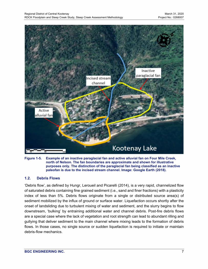
The term “paleofan” is used to describe portions of fans interpreted as no longer active (under present climate and geomorphic/geological setting) and entirely removed from channel processes (i.e., with negligible potential for channel avulsion and flow propagation) due to deep channel incision (Kellerhals & Church, 1990).
Paraglacial fans are located throughout the RDCK. These are defined as fans primarily deposited shortly after the landscape was deglaciated (Ryder, 1971a; 1971b; Church & Ryder, 1972). Paraglacial fans are found as elevated surfaces near the mouth of steep creeks at the modern-day fan apex in RDCK (e.g., at Eagle Creek and Duhamel Creek). Under specific circumstances, paraglacial fans could reactivate (e.g., Figure 1-5).
Regional District of Central Kootenay March 31, 2020 RDCK Floodplain and Steep Creek Study, Steep Creek Assessment Methodology Project No.: 0268007
BGC ENGINEERING INC. 7
Figure 1-5. Example of an inactive paraglacial fan and active alluvial fan on Four Mile Creek,
north of Nelson. The fan boundaries are approximate and shown for illustrative purposes only. The distinction of the paraglacial fan being classified as an inactive paleofan is due to the incised stream channel. Image: Google Earth (2018).
1.2. Debris Flows
‘Debris flow’, as defined by Hungr, Leroueil and Picarelli (2014), is a very rapid, channelized flow of saturated debris containing fine grained sediment (i.e., sand and finer fractions) with a plasticity index of less than 5%. Debris flows originate from a single or distributed source area(s) of sediment mobilized by the influx of ground or surface water. Liquefaction occurs shortly after the onset of landsliding due to turbulent mixing of water and sediment, and the slurry begins to flow downstream, ‘bulking’ by entraining additional water and channel debris. Post-fire debris flows are a special case where the lack of vegetation and root strength can lead to abundant rilling and gullying that deliver sediment to the main channel where mixing leads to the formation of debris flows. In those cases, no single source or sudden liquefaction is required to initiate or maintain debris-flow mechanics.

Regional District of Central Kootenay March 31, 2020 RDCK Floodplain and Steep Creek Study, Steep Creek Assessment Methodology Project No.: 0268007
BGC ENGINEERING INC. 8
Sediment bulking is the process by which rapidly flowing water entrains bed and bank materials either through erosion or preferential “plucking” until sediment saturation is reached (often at 60-70% sediment concentration by volume). At this time, further sediment entrainment may still occur through bank undercutting and transitional deposition of debris, with a zero-net change in sediment concentration. Bulking may be limited to partial channel substrate mobilization of the top gravel layer, or – in the case of debris flows – may entail entrainment of the entire loose channel debris. Scour to bedrock in the transport zone is expected in the latter case.
Unlike debris avalanches, which travel on unconfined slopes, debris flows travel in confined channels bordered by steep slopes. In this environment, the flow volume, peak discharge, and flow depth increase, and the debris becomes sorted along the flow path. Debris-flow physics are highly complex and video recordings of events in progress have demonstrated that no unique rheology can describe the range of mechanical behaviour observed (Iverson, 1997). Flow velocities typically range from 1 to 10 m/s, although very large debris flows from volcanic edifices, often containing substantial fines, can travel at more than 20 m/s along much of their path (Major et al., 2005). The front of the rapidly advancing flow is steep and commonly followed by several secondary surges that form due to particle segregation and upwards or outwards migration of boulders. Hence, one of the distinguishing characteristics of coarse granular debris flows is vertical inverse grading, in which larger particles are concentrated at the top of the deposit. This characteristic behaviour leads to the formation of lateral levees along the channel that become part of the debris-flow depositional legacy. Similarly, depositional lobes are formed where frictional resistance from unsaturated coarse-grained or large organic debris-rich fronts is high enough to slow and eventually stop the motion of the trailing liquefied debris. Debris-flow deposits remain saturated for some time after deposition but become rigid once seepage and desiccation have removed pore water.
Coarse granular debris flows require a channel gradient of at least 27% (15o) for transport over significant distances (Takahashi, 1991) and have volumetric sediment concentrations in excess of 50%. Between the main surges a fluid slurry with a hyperconcentration (>10%) of suspended fines occurs. Transport is possible at gradients as low as 20% (11o)2, although some type of momentum transfer from side-slope landslides is needed to sustain flow on those slopes. Debris flows may continue to run out onto lower gradients even as they lose momentum and drain: the higher the fine grained (especially clay) sediment content, and hence the slower the sediment-water mixture will lose its pore water, the lower the ultimate stopping angle. The clay fraction is the most important textural control on debris-flow mobility. The surface gradient of a debris-flow fan approximates the stopping angle for flows issuing from the drainage basin.
Due to their high flow velocities, peak discharges during debris flows are at least an order of magnitude larger than those of comparable return period floods and can be 50 times larger or more (Jakob & Jordan, 2001; Jakob et al., 2016). Further, the large caliber of transported
2 For volcanic debris flows, transport can occur at even lower gradients.

Regional District of Central Kootenay March 31, 2020 RDCK Floodplain and Steep Creek Study, Steep Creek Assessment Methodology Project No.: 0268007
BGC ENGINEERING INC. 9
sediment and wood means that debris flows are highly destructive along their channels and on fans.
Channel banks can be severely eroded during debris flows, although lateral erosion is often associated with the trailing hyperconcentrated flow phase that is characterized by lower volumetric sediment concentrations. The most severe damage results from direct impact of large clasts or coarse woody debris against structures that are not designed for the impact forces. Even where the supporting walls of buildings may be able to withstand the loads associated with debris flows, building windows and doors are crushed and debris may enter the building, leading to extensive damage to the interior of the structure (Jakob et al., 2012). Similarly, linear infrastructure such as roads and railways are subject to complete destruction. On the medial and distal fan (the lower 1/3 to 2/3), debris flows tend to deposit their sediment rather than scour. Therefore, exposure or rupture of buried infrastructure such as telecommunication lines or pipelines is rare. However, if a linear infrastructure is buried in the proximal fan portions that undergo cycles of incision and infill, or in a recent debris deposit, it is likely that over time or during a significant runoff event, the tractive forces of water will erode through the debris until an equilibrium slope is achieved, and the infrastructure thereby becomes exposed or may rupture due to boulder impact or abrasion. This necessitates understanding the geomorphic state of the fans being traversed by a buried linear infrastructure.
Channel avulsion occurs when the creek migrates out of an existing channel and forms a new channel. Avulsions are likely in poorly confined channel sections (particularly on the outside of channel bends where debris flows tend to super-elevate). Sudden loss of confinement and decrease in channel slope cause debris flows to decelerate, drain their inter-granular water, and increase shearing resistance, which slow the advancing bouldery flow front and block the channel. The more fluid afterflow (hyperconcentrated flow) is then often deflected by the slowing front, leading to secondary avulsions and the creation of distributary channels on the fan. Because debris flows often display surging behaviour, in which bouldery fronts alternate with hyperconcentrated afterflows, the cycle of coarse bouldery lobe and levee formation and afterflow deflection can be repeated several times during a single event. These flow aberrations and varying rheological characteristics pose a challenge to numerical modelers seeking to create an equivalent fluid (Iverson, 2014).
1.3. Debris Floods
Within the past 20 years the English term ‘debris flood’ has come into use to describe severe floods involving exceptionally high rates of transport as bedload of coarse sediments, usually occurring in steep channels (Hungr, Evans, Bovis & Hutchinson, 2001; Wilford, Sakals, Innes, Sidle & Bergerud, 2004). Specific classifications have been proposed much earlier in Europe (Stiny, 1931; Aulitzky, 1980) using the German terms “murstossfähige-, murfähige, geschiebeführende and hochwasserführende Wildbäche”. This was translated by G. Eisbacher into “debris-flow”, “debris flood”, “bedload transporting” and “flood” creeks. The first two terms are somewhat confusing as they translate directly into “debris-flow (mur), surge/push (stoss), capable (fähig)” and “debris-flow capable”. Hence the only difference is the term “stoss”. The absence or

Regional District of Central Kootenay March 31, 2020 RDCK Floodplain and Steep Creek Study, Steep Creek Assessment Methodology Project No.: 0268007
BGC ENGINEERING INC. 10
presence of surges is not a sufficiently discriminatory criterion between debris flows and debris floods and could only be distinguished if the event is observed in action.
The English term “debris flood” is favored by geotechnical engineers and engineering geomorphologists who share responsibility to protect society and its infrastructure from such events. A recent authoritative review of landslide-like phenomena defines debris flood as “very rapid flow of water, heavily charged with debris, in a steep channel. Peak discharge is comparable to that of a water flood.” (Hungr et al., 2014: p.185). The text continues: “the stream bed may be destabilized causing massive movement of sediment. Such sediment movement (sometimes referred to as “live bed” or “carpet flow” by hydraulicians) can reach transport rates far exceeding normal bed load movement through rolling and saltation. However, the movement still relies on the tractive forces of water.” (Hungr et al., 2014). Accordingly, debris floods represent water driven flood flows with high bedload transport of gravel to boulder size material and significant damage potential. Unfortunately, in much of the technical literature they remain classified as hyperconcentrated flows, a quite different phenomenon. However, BGC defines debris floods more precisely in the following paragraphs.
Bedload transport in gravel-bed channels has been characterized in three stages (Carling, 1988; Ashworth & Ferguson, 1989). In stage 1, fine material – typically sand – overpasses a static bed or is mobilised by winnowing from an otherwise static bed. The force of the flowing water is insufficient to mobilize the local bed material. In stage 2, local bed material is entrained and redeposited at low rates. Individual clasts are mobilised from the bed surface independently of other entraining events (except when movement of a relatively large clast liberates finer material that was hiding in its shadow). Most of the bed remains stable most of the time (a state defined as “partial transport” by Wilcock and McArdell (1993)). In stage 3, the entire streambed or a continuously connected portion of it becomes mobile and activity may extend to a depth of several median grain sizes below the surface as the result of momentum transfer by grain-grain collisions. In many instances, the channel itself is modified by erosion and sedimentation. A debris flood is, then, a case of stage 3 transport.
Debris floods are relatively rare because stage 3 transport is rare in gravel-bed channels. In such channels, where bed and banks consist of similar non-cohesive materials the banks are readily eroded due to inherent weakness and the gravitational assist (Lane, 1955) so that the channel widens, with consequent reduction in flow depth, until the flow is just able to transport the incoming bed material load at rates near the threshold for transport and near-bank currents are no longer effective (Parker, 1978; 1979). The shear force exerted by the flow on the bed remains near the threshold value for entrainment of the bed material. Debris floods occur when this condition is exceeded. Steep mountain channels (in which the width remains limited because the banks consist of rock or other non-erodible material) may experience stage 3 flow and debris flood relatively frequently (every few years; cf. Theule, Liébault, Laigle, Love & Jaboyedoff, 2015). Larger, but still relatively steep, channels carrying extraordinary floods (floods of order 100-year return period or greater) also are prone to debris flood occurrence. Such floods are distinctly two-phase flows, with ‘clear water’ or water with a substantial suspended sediment load, overlying a slurry-like flow – characterised as an “incipient granular mass flow” by Manville and White (2003)
Regional District of Central Kootenay March 31, 2020 RDCK Floodplain and Steep Creek Study, Steep Creek Assessment Methodology Project No.: 0268007
BGC ENGINEERING INC. 11
– containing a high concentration of bed material, the finest fractions of which may be episodically suspended.
For practical purposes we define a debris flood as “a flood during which the entire bed, possibly barring the very largest blocks, mobilizes for at least a few minutes and over a length scale of at least ten times the channel width”.
Debris floods typically occur on creeks with channel gradients between 5 and 30% (3-17o), but in contrast to common belief, can also occur on lower gradient gravel bed rivers. Due to their initially relatively low sediment concentration, debris floods can be more erosive along low-gradient alluvial channel banks than debris flows. Bank erosion and excessive amounts of bedload introduce large amounts of sediment to the fan where they accumulate (aggrade) in channel sections with decreased slope. Debris floods can be initiated on the fan itself through rapid bed erosion and entrainment of bank materials, as long as the stream power is high enough to transport clasts larger than the median grain size (D50). Because typical long-duration storm hydrographs fluctuate several times over the course of the storm, several cycles of aggradation and remobilization of deposited sediments on channel and fan reaches can be expected during the same event (Jakob et al., 2016). Similarly, debris floods triggered by outbreak floods may lead to single or multiple surges irrespective of hydrograph fluctuations that can lead to cycles of bank erosion, scour and infill. This is important for interpretations of field observations as only the final deposition or scour can be measured. This is relevant where a pipeline or telecommunication line is to be buried. Maximum scour during a debris flood may be much deeper than what is viewed and measured during a field visit.
Church and Jakob (2020) developed a three-fold typology for debris floods, which have previously not been defined well. This is summarized in Table 1-1. Identifying the correct debris-flood type is key in preparing for numerical modelling and hazard assessments. Type 1 is considered in clearwater flood on fan process described in Section 1.4, due to similar regional scale characteristics. Type 2 debris floods are generated from diluted debris flows. Type 3 are generated by natural or man-made dam breaches.
Hyperconcentrated flows are a special case of debris floods that are typical for volcanic sources areas or fine-grained sedimentary rocks. They can occur as Type 1, 2 or 3 debris floods. The term “hyperconcentrated flow” was defined by Pierson (2005) on the basis of sediment concentration as “a type of two-phase, non-Newtonian flow of sediment and water that operates between normal discharge (water flow) and debris flow (or mudflow)”. The use of the term “hyperconcentrated flow” should be reserved for volcanic or weak sedimentary fine-grained slurries.

Regional District of Central Kootenay March 31, 2020 RDCK Floodplain and Steep Creek Study, Steep Creek Assessment Methodology Project No.: 0268007
BGC ENGINEERING INC. 12
Table 1-1. Debris-flood classification based on Church and Jakob (2020).
Term Definition
Typical sediment
concentration by volume
(%)
Typical Qmax factor compared to
calc. clearwater Physical Characteristics Typical impacts
Typical return period range
(years) Type 1 (Meteorologically-generated debris flood)
Rainfall/snowmelt generated through exceedance of critical shear stress threshold when most of the surface bed grains are being mobilized. While not a fixed threshold, the 1SD bed surface grains are a reasonable proxy for major channel shifts.
< 5 1.02 to 1.2 (depending on the proximity of major debris sources to the fan apex as well as organic debris loading)
Steep fans (1 to 10%), shallow but wide active floodplain widespread boulder carpets, clast to matrix-supported sediment facies, subrounded to rounded stones, some imbrication, disturbed riparian vegetation, frequent fan avulsions
Widespread bank instability, avulsions, alternating reaches of bed aggradation and degradation, blocked culverts, scoured bridge abutments, damaged buried infrastructure particularly in channel reaches u/s of fans
>10
Type 2 (Debris flow to debris flood dilution)
Transitional as a consequence of debris flows. Substantially higher sediment concentration compared to a Type 1 debris flood and accordingly greater facility to transport larger volumes of sediment. All grain calibers mobilized, except from lag deposits (big glacial or rock fall boulders)
< 50 Depends on the distance of the debris-flow transition to the area of interest. Unless a debris-flow tributary feeds directly into the fan apex, bulking is up to 1.5.
As for Type 1 but rarely clast-supported and with higher matrix sediment concentration. Stones subangular to angular, boulder carpets on fans often display sharp edges
Widespread bank instability, avulsions, substantial bed aggradation particularly on fans, blocked culverts, scoured bridge abutments, damaged buried infrastructure on fans
>50
Type 3 (Outbreak floods)
Outbreak flood in channels with insufficient steepness for debris-flow generation. Critical shear stress for debris-flood initiation exceeded abruptly due to sharp hydrograph associated with the outbreak flood. All Ds mobilized in channel bed and non-cohesive banks
< 10 (except
immediately downstream of the outbreak)
Up to 100 depending on size of dam and distance to dam failure, Qmax should be calculated by combination of dam breach analyses and flood routing
Presence or deduction of landforms that could lead to eventual outbreak floods, Watershed channel reaches with distinct trimlines in case of past events. pronounced superelevation in channel bends, even aged vegetation on large segments of the fan, high fines content in matrix, sometimes inverse grading
Vast bank erosion, avulsions, substantial bed degradation along channels and aggradation on fans, destroyed culverts, outflanked or overwhelmed bridges, damaged buried infrastructure on channels and fans
>100 (can be singular
events in the case of a moraine dam or glacial
breach)

Regional District of Central Kootenay March 31, 2020 RDCK Floodplain and Steep Creek Study, Steep Creek Assessment Methodology Project No.: 0268007
BGC ENGINEERING INC. 13
1.4. Clearwater Floods on Alluvial Fans
Clearwater floods are defined as “riverine and lake flooding resulting from inundation due to an excess of clearwater discharge in a watercourse or body of water such that land outside the natural or artificial banks which is not normally under water is submerged”. Note that for most creeks in the RDCK study area, a water depth sufficient to submerge land outside the creek banks is – by Church and Jakob’s (2020) definition – a Type 1 debris flood. Hence, clearwater floods are likely to occur at low return periods.
Most of the severe flooding in the RDCK occurs between May and June due to snow melt (freshet). In contrast to other areas in BC, flooding is not typically driven solely by intense winter rainstorms or rain-on-snow events. Flood severity can vary considerably depending on:
• The amount and duration of the precipitation (rain and snowmelt) event • The antecedent moisture condition of the soils • The size of the watershed • The floodplain topography • The effectiveness and stability of flood protection measures.
For example, excessive rainfall, rain-on-snow, or snowmelt can cause a stream or river to exceed its natural or engineered capacity. Overbank flooding occurs when the water in the stream or river exceeds the banks of the channel and inundates the adjacent floodplain in areas that are not normally submerged (Figure 1-6). Climate change also has the potential to impact the probability and severity of flood events by augmenting the frequency and intensity of rainfall events, altering snowpack depth, distribution, timing, snow water equivalent (SWE), and freezing levels and causing changes in vegetation type, distribution and cover. Impacts are likely to be accentuated by increased wildfire activity and / or insect infestations (British Columbia Ministry of Environment [BC MOE], 2016).
Figure 1-6. Conceptual channel cross-section in a typical river valley.
In BC, the 200-year return period flood is used to define floodplain areas, except for Fraser River, where the 1894 flood of record is used, corresponding to an approximately 500-year return period (Engineers and Geoscientists BC [EGBC], 2017). The 200-year flood is the annual maximum river

Regional District of Central Kootenay March 31, 2020 RDCK Floodplain and Steep Creek Study, Steep Creek Assessment Methodology Project No.: 0268007
BGC ENGINEERING INC. 14
flood discharge (and associated flood elevation) that is exceeded with an annual exceedance probability (AEP) of 0.5% or 0.005. While flooding is typically associated with higher return events, such as the 200-year return period event, lower return period events (i.e., more frequent and smaller magnitude events) have the potential to cause flooding if the banks of the channel are exceeded.

Regional District of Central Kootenay March 31, 2020 RDCK Floodplain and Steep Creek Study, Steep Creek Assessment Methodology Project No.: 0268007
BGC ENGINEERING INC. 15
2. STEEP CREEK HAZARD ASSESSMENT METHODS FOR DEBRIS-FLOOD PRONE CREEKS
2.1. Introduction
This section summarizes the methods employed by BGC to characterize hazard processes, determine the frequency and magnitude of steep creek hazards, model flood inundation, and compile hazard maps.
2.2. Hazard Assessment Methods Background
This section introduces steep creek hazard assessment for readers who may be new to this type of analysis. The specific hazard assessment methods are described in Sections 2.3 and following.
2.2.1. Frequency-Magnitude Relationships
Frequency-magnitude (F-M) relations answer the question “how often and how big can steep creek hazard events become?”. The ultimate objective of an F-M analysis is to develop a graph that relates the return period of the hazard to its magnitude (e.g., peak discharge or sediment volume). Figure 2-1 shows this conceptually. The red line (i.e., event magnitude) levels off at some point because of either sediment supply or water limitations. This means that debris flows and debris floods from a given watershed have a maximum possible sediment volume and peak discharge. In some cases, a secondary process may act at a higher return period, in which case an additional frequency curve needs to be juxtaposed.
Any F-M calculation that spans time scales of millennia necessarily includes some judgment and assumptions, both of which are subject to some degree of uncertainty. Quantification of this uncertainty is often difficult, and judgement is required to assess the appropriate degree of conservatism, particularly when life loss risk and mitigation design are involved. Design decisions are also complicated by a changing climate as it affects the frequency-magnitude relationships of steep creek processes.

Regional District of Central Kootenay March 31, 2020 RDCK Floodplain and Steep Creek Study, Steep Creek Assessment Methodology Project No.: 0268007
BGC ENGINEERING INC. 16
Figure 2-1. Conceptual frequency-magnitude curve for two different processes (i.e., debris flows
in green and debris floods in red showing larger event occur more rarely).
Once events have been documented and their age and volume estimated, return period ranges need to be assigned to individual events that allow extrapolation and interpolation into annual probabilities beyond those extracted from the physical record. Such record extension is necessary to develop quasi-continuous event scenarios that then form the basis of numerical flood modeling and to cover the entire range of events apt to occur and for which one may wish to provide mitigation.
2.2.2. Return Period Classes
This report uses the terms “frequency”, “hazard probability” and “return period” interchangeably, depending on the context. Frequency is numerically equivalent to long-term hazard probability. It is defined as the annual probability of occurrence of a hazard scenario. Return period is the inverse of frequency, and it is defined as the average recurrence interval (in years) between hazardous events of the same magnitude. For example, an annual frequency of 0.01 corresponds to a 100-year return period.
Four return period classes were defined for the work (per BGC, November 15, 2019). Table 2-1 outlines return periods considered in steep creek hazard assessment numerical modelling and hazard maps. The return periods are intended to:
• Span a spectrum of event magnitudes that can be reasonably estimated with the information available
• Support the implementation of standards-based flood management policies and bylaws • Support risk assessment that may be completed under future scopes of work.

Regional District of Central Kootenay March 31, 2020 RDCK Floodplain and Steep Creek Study, Steep Creek Assessment Methodology Project No.: 0268007
BGC ENGINEERING INC. 17
The table displays “return period ranges” and “representative return periods”. The representative return periods fall close to the mean of each range3. Given uncertainties, they generally represent the spectrum of event magnitudes within the return period ranges.
Table 2-1. Return period classes.
Return Period Range (years)
Representative Return Period
(years)
10-30 20
30-100 50*
100-300 200
300-1000 500*
These classes correspond to those recommended in the legislated flood assessments guidelines by Engineers and Geoscientists British Columbia (EGBC, 2018).
Hazards associated with higher return periods (i.e., >1000 years) were not considered, as they are associated with very high uncertainty and are typically outside the range of dating methods that can be applied to such steep creek hazard and risk studies.
2.3. Hazard Assessment Workflow
The flowchart shown in Figure 2-2 outlines the workflow for the hazard assessment portion of the project. The key points of the hazard assessment are outlined below.
• The desktop study and field investigation form part of the basis of the Hazard Process Characterization.
• The main objective of the Hazard Process Characterization is to develop a relationship for frequency and peak discharge/sediment volume.
• This in turn is part of the input to the Spatial Hazard Characterization where numerical models (HEC-RAS and FLO-2D) are used to simulate floods and debris floods for each modelling scenario.
• Modeling results from each scenario are combined into hazard maps.
The Hazard Process Characterization is split into four subsections: Section 2.4.1 addresses the desktop study, Section 2.4.2 addresses field investigation and data processing steps, the frequency-discharge assessment is presented in Section 2.5.2, and Section 2.5.3 addresses the frequency-sediment volume relationship.
3 The 50- and 500- year events do not precisely fall at the mean of the return period ranges shown in Table 2-1 but
were chosen as round figures due to uncertainties and because these return periods have a long tradition of use in BC.

Regional District of Central Kootenay March 31, 2020 RDCK Floodplain and Steep Creek Study, Steep Creek Assessment Methodology Project No.: 0268007
BGC ENGINEERING INC. 18
Figure 2-2. Workflow applied for flood and debris flood prone steep creeks for developing
frequency-magnitude relationships, modelling, and preparing hazard maps.

Regional District of Central Kootenay March 31, 2020 RDCK Floodplain and Steep Creek Study, Steep Creek Assessment Methodology Project No.: 0268007
BGC ENGINEERING INC. 19
2.4. Basis for Hazard Process Characterization
The desktop study and field investigation form part of the basis of the Hazard Process Characterization. The methods used for these two components are described below.
2.4.1. Desktop Study
2.4.1.1. Historical Records Review
BGC reviewed historical engineering reports, scientific literature and local historical records to identify past debris flow, debris flood and/or flood events. Although flooding on nearby creeks does not necessarily imply flooding on the creek of interest, this information helped guide the frequency analysis.
The Ministry of Forests, Lands, Natural Resource Operations and Rural Development (MFLNRORD) provided excerpts from their so-called “complaints database” for each creek in this assessment. The database contains details and observations on events that occurred, or assessments that were undertaken. The database provided valuable insights to events and developments on creeks.
BGC contacted local archives and museums and gathered historic accounts of events.
Twitter data from Drive BC announcements by the BC Ministry of Transportation and Infrastructure for road closures or similar events were also analyzed.
Historical records from the various sources described above were compiled into a database by BGC and summarized in a historic timeline for each creek with references.
2.4.1.2. Air Photo Review
Air photos were reviewed to:
• Delineate shifts in creek alignment over time • Estimate the frequency and deposit area of past hydrogeomorphic4 events and to assess
avulsion hazards • Estimate bank erosion.
Sizable debris flows or debris floods on mountain creeks can kill vegetation in the affected area or obliterate it in areas of high flow velocity. If such events are sufficiently large, a cover of debris deposits can be identified as light grey or white on monochromatic or colour air photographs. In areas where debris flows or debris floods have not destroyed tree stands, dense tree canopies can obscure such deposits, which are then difficult to identify in absence of detailed ground investigations (e.g., dendrochronology, trenching). Additionally, avulsions could cause the channel to leave its present position and flow overland somewhere else on the fan. Historical avulsion channels can be identified in historical air photos using similar techniques. The locations
4 In this context, hydrogeomorphic events are debris floods and debris flows, as well as bank erosion and sediment
inundation.
Regional District of Central Kootenay March 31, 2020 RDCK Floodplain and Steep Creek Study, Steep Creek Assessment Methodology Project No.: 0268007
BGC ENGINEERING INC. 20
of historical channels can also be detected in a LiDAR digital elevation model (DEM) as described in Section 2.4.1.3.
A series of historical air photos was obtained from government sources at varying scales. The air photos were orthorectified using a geographic information system (GIS). A higher density of control points near alluvial fans is used to minimize distortion during the orthorectification process. BGC estimated the spatial accuracy afforded by application of these methods to be about +/- 10 m, as air photos were not flown specifically for these sites, and because of distortion associated with air photos of terrain with high relief.
Where sediment deposition was interpreted to have occurred, areas were delineated with polygons. Estimates of historic bank erosion were obtained by measuring the widening of the creek at locations of interest. The results were used to calibrate the bank erosion model. Other changes such as land use, road construction, logging and fire history were also noted.
2.4.1.3. LiDAR Review
Airborne LiDAR, which stands for Light Detection and Ranging, is a remote sensing method that uses laser pulses sent from a sensor mounted on an aircraft to measure ranges (i.e., variable distances) to the Earth. These light pulses – combined with other data recorded by the airborne system – generate precise, three-dimensional information about the shape of the Earth and its surface characteristics. The data can be processed into so called “bare-earth” surfaces where all the vegetation is removed from the data to represent the topographic ground surface.
LiDAR is used to identify historical channels or deposits on the fan, while the surface in the watershed is used to identify geomorphic features that might otherwise be obscured by vegetation in satellite imagery or air photographs. Such features may be tell-tale signs of previous or possible future landslides that need to be accounted for in a detailed hazard assessment.
2.4.2. Field Investigation
Field work was conducted by BGC personnel in summer 2019, and included field mapping, test pitting, coring of trees for dendrogeomorphic analysis, and channel hikes to collect high water mark cross sections and grainsize distributions. The fan and upper watersheds of all the study creeks were also traversed by helicopter on July 6, 2019 and photographs were taken by Matthias Busslinger, P.Eng. (BC), M.A.Sc., Dr. Matthias Jakob, Ph.D., P.Geo. (BC) and Marc-Olivier Trottier, P.Eng. (BC), M.A.Sc.
2.4.2.1. Field Mapping
Field observations were recorded with handheld tablet computers, including GPS locations. ArcCollector software by ESRI, a GIS based software was used for data management. Tablets were used for navigating and data collection. Each tablet computer had various map layers loaded including field mapping targets, a DEM, and satellite imagery. Collected information was uploaded daily to BGC’s servers. Collected information included: general observations, photographs, oral accounts by residents, channel characteristics, dimensions of bridge and culvert openings, high water marks, deposits, potential avulsion points, test pit locations (see Section 2.4.2.2),
Regional District of Central Kootenay March 31, 2020 RDCK Floodplain and Steep Creek Study, Steep Creek Assessment Methodology Project No.: 0268007
BGC ENGINEERING INC. 21
dendrogeomorphological observations (see Section 2.4.2.3), and grainsize distribution (see Section 2.4.2.4).
2.4.2.2. Test Trenching and Radiocarbon Dating
Test trenching allows estimation of the thickness of past debris flows/debris floods, which are typically distinct from overlying and underlying deposits. It also permits sampling of datable organic materials found in paleosols (old soil layers) and embedded within the event deposits. An approximate age can then be assigned to the deposit.
Radiocarbon dating involves measuring the amount of the radioisotope 14C preserved in organic materials and using the rate of radioactive decay to calculate the age of a sample. This method requires the deposition and preservation of organic materials within the sedimentary stratigraphy of the fan. The age range of this method is from approximately 45,000 years to several decades before present. As such, the method is applicable to the time scale of post-glacial fan formation in western Canada.
Test pits were excavated by backhoe on two of the study creeks: Eagle Creek and Harrop Creek fans. At Eagle Creek, five test pits were excavated on July 25, 2019. Additionally, a trench was open for waterline works that BGC traversed and logged intermittently on July 25, 2019. At Harrop Creek, five test pits were excavated on July 9, 2019. Test pits were dug on each fan typically to about 2 m depth, the pit walls were logged, and photos taken at each location.
Unit contacts and buried soils were examined for organic carbon for radiocarbon dating. Test pits and exposures were photographed. Radiocarbon samples were collected in plastic bags, air-dried, and then sent to Beta Analytics in Florida for age determination by Accelerator Mass Spectrometry (AMS).
Results from the radiocarbon were reviewed to identify unique events on each creek. Results from test trenching and radiocarbon dating were used to inform the frequency assessment of hydrogeomorphic events on the fan, sediment deposit thickness for modelling, as well as to cross-check sediment volume estimates described in Section 2.5.3.
2.4.2.3. Dendrogeomorphology
Dendrogeomorphology is a subdiscipline of dendrochronology, in which tree rings and tree growth are used to analyze historic landslide activity. Dendrogeomorphology analysis is based on two main characteristics of tree ring samples:
1. Tree age: the age of the tree determines the “minimum establishment date”: in other words, the approximate time when the tree started growing. • The date is a minimum, because tree rings indicate the minimum age of the tree at the
height where the coring was collected. Cores are usually collected at approximately chest height (1.2 m), so it may have taken the tree a few years to grow 1.2 m. In addition, several years may pass for a tree seed to establish on a freshly disturbed surface.

Regional District of Central Kootenay March 31, 2020 RDCK Floodplain and Steep Creek Study, Steep Creek Assessment Methodology Project No.: 0268007
BGC ENGINEERING INC. 22
• If many trees in one area all started growing around the same time, this may indicate that a stand-destroying event occurred that cleared the original trees and left space for new trees to establish.
2. Special features (in conifers only): Features in the wood that may suggest landslide activity include scars, traumatic resin ducts (TRDs), reaction wood and growth disturbances. • Scars occur when a landslide or avalanche damages the bark or wood of a tree but
doesn’t kill the tree. Figure 2-3 shows an example of a debris-flow scarred tree. • TRDs are small circles that appear within the wood, which indicate that the tree
sustained damage during that year (similar to scar tissue). • Reaction wood appears when a tree has been knocked or tipped over by a landslide.
Denser wood grows on the downslope side, to correct the growth of the tree and ensure that it continues to grow vertically.
• Growth disturbances occur when a landslide changes the conditions around the tree, such as the availability of light, water or nutrients. These changes may cause the tree to grow noticeably faster or slower.
Tree cores were extracted from living trees using a 5 mm increment borer. In the office, the samples were glued onto wooden mounting boards and sanded to facilitate ring and feature identification. Analysis was completed using a specialized scanner and WinDENDRO software (Regent Instruments Inc., 2012). WinDENDRO is a semi-automatic image analysis program, which identifies tree rings and measures the width of the yearly growth. Once the tree ages were confirmed, the growth rings were analyzed to identify anomalies that may be associated with debris flood, debris flow or avalanche events. It can be difficult to differentiate between steep creek and avalanche processes, although sometimes, the location of the TRDs within the ring can indicate whether the damage occurred in the dormant period (winter) or the growing season (spring and summer).
Figure 2-3. Impact scars on a spruce tree near Fergusson Creek in southwest BC showing an
example of scars that can be dated precisely. The red arrow points at a scar, and the blue arrow points at the center of the tree (from Jakob, 1996).
Where possible, results of the dendrogeomorphologic analysis were used to confirm ages of deposits or supplement F-M relationships as established from other methods.

Regional District of Central Kootenay March 31, 2020 RDCK Floodplain and Steep Creek Study, Steep Creek Assessment Methodology Project No.: 0268007
BGC ENGINEERING INC. 23
2.4.2.4. Bed Material Sampling
Bed material sampling was conducted in each creek to support sediment transport and flow resistance estimates. Sampling was typically conducted on the fan at 2 to 3 locations along the channel to characterize downstream variability. Sampling was conducted by photographic and stone count methods, both of which characterize the surficial bed material characteristics, which is typically coarser than subsurface conditions.
Stone counts followed the Wolman (1954) method to determine sediment size distribution at each site. In this method, a flexible tape measure is laid on the sampling area and a random stone is selected at set intervals (every 20- 30 cm in this project). The intermediate axis (b-axis) of the selected grain is measured. Based on the measured value, the grain was binned into ½ phi size-classes and the number of grains measured within each grade class is recorded. Phi classes are a logarithmic classification where, phi = -log2D and D is the grain diameter (e.g., if D is 32 mm, phi is -5, if D is 45 mm, phi is -5.50). Approximately 100 grains are measured at each sampling location. An example result is presented on Figure 2-4.
Photographic samples were collected concurrently with the stone counts and simply involved placing a scale object on the stream bed (in this case a soccer ball with a diameter of approximately 220 mm) and collecting oblique photos. These photos provided a qualitative description of the spatial variability of bed material conditions, which is not characterized by the stone counts.
Figure 2-4. Redfish Creek sediment distribution at Redfish 1 (downstream of fan apex) from
Wolman Count data.
0
20
40
60
80
100
0
10
20
30
40
50
<2 2.8 4 5.6 8 11 16 22 32 45 64 90 128 180 256 >256
Perc
ent f
iner
than
(%)
Perc
ent i
n cl
ass
(%)
Particle Size (mm)Percent in class Percent finer than

Regional District of Central Kootenay March 31, 2020 RDCK Floodplain and Steep Creek Study, Steep Creek Assessment Methodology Project No.: 0268007
BGC ENGINEERING INC. 24
2.5. Hazard Process Characterization
Hazard process characterization involves identifying active hydrogeomorphic processes that impact the fan (process characterization) and establishing frequency-magnitude (peak discharge and sediment volume) relations for floods, debris floods and debris flows.
2.5.1. Process Characterization
Debris flows can be separated from debris floods and floods through a variety of diagnostic techniques which were combined in this work. Three levels of process identification can be differentiated: the character of the contributing drainage basin, characteristics of the impacted channel, and characteristics of prior deposits at the basin mouth.
2.5.1.1. Drainage Basin
Floods carrying very large sediment loads (debris floods; hyperconcentrated flows) and debris flows originate in steep channels in upland and montane regions. Wilford et al. (2004) presented a discriminant diagram based on the length and ‘Melton ratio’ of the drainage basin to identify basins susceptible to each type of extreme flow. The Melton ratio is the dimensionless quotient of drainage relief (H) and area (A), i.e., H/√A, a measure of the steepness of the basin. Since the original presentation, many data have been added to the diagram (Figure 2-5). While it still provides a first order discrimination of debris flood and debris flow locale, it is not an assured means for correct process classification. The diagram remains useful for first reconnaissance based on map work. A key consideration is sediment availability which, in regions with former Quaternary glaciation, occurs as till, and glaciofluvial, glaciolacustrine or glaciomarine sediments. In those regions, the exposure of mobilizable sediment is augmented by continued downcutting of the streams into sediments or bedrock to adjust to postglacial base levels. Sediment replenishment to the stream channel is particularly pronounced in regions with active tectonic uplift and high precipitation (Burbank & Anderson, 2011), as well as in valleys with rapid glacial retreat (Ballantyne, 2002).

Regional District of Central Kootenay March 31, 2020 RDCK Floodplain and Steep Creek Study, Steep Creek Assessment Methodology Project No.: 0268007
BGC ENGINEERING INC. 25
Figure 2-5. Steep creek processes as a function of Melton Ratio and stream length. Process
boundaries are from fans in Alberta and BC (Holm et el., 2016; Lau, 2017). The grouping of classes as shown in the dashed-line delineated bubbles is done by eye and somewhat arbitrary. Some creeks are also subject to more than one process.
2.5.1.2. Stream Channel
Stream channels subject to debris floods may be artificial or natural. Their gradient can vary widely but will be below that of debris flow-prone systems, typically below approximately 30% slope. The calibre of the entrained sediment and the state of the channel bed determine whether, for a particular high runoff, a debris flood occurs. Channels that have recently been subjected to a debris flood may be scoured or may contain alternating reaches of rock and boulder debris. But often sediment is deposited during the falling limb of the hydrograph, a phenomenon that challenges reliable reconstruction of cross-sectional areas to back-calculate peak discharge once flow velocities have been estimated. Extensive bank erosion may signal debris flood occurrence as major bank erosion is associated with the mobilization of the D84 5or larger clasts.
2.5.1.3. Deposits
Sediment deposits provide key discriminating criteria. While debris flow deposits may either remain entirely unsorted or exhibit inverse grading, debris flood deposits are stratified and imbricated in the manner of normal fluvial deposits. However, sand content is usually much higher than in ‘normal’ fluvial deposits due to the rapidity of deposition and less effective sorting (Blair & McPherson, 1994). Depending on sediment source, deposits may be largely sandy with matrix supported gravel with neither normal nor inverse grading (Figure 2-6). In some cases, it is challenging to differentiate different debris flood events due to the lack of grading or interbedded
5 D84 denotes the 84th percentile of the stone count distribution, implying only 16% of the sample are larger.

Regional District of Central Kootenay March 31, 2020 RDCK Floodplain and Steep Creek Study, Steep Creek Assessment Methodology Project No.: 0268007
BGC ENGINEERING INC. 26
paleosols that often are eroded in subsequent events. However, subtle textural and sharp grading changes may suggest a different event. Similarly, particularly old deposits may be differentiable through oxidization or cementation, for example, in carbonate rocks (limestone and dolomite).
Unlike debris flow deposits, which are often sharply bounded with an abrupt debris snout, debris flood deposits consist of sheets of gravel, often with small distributary channels incised into them. Observations by eye witnesses and a variety of short amateur movies (e.g., on YouTube under the term “debris flood” or “flash flood”) show that the sheets of mobile sediment, once avulsed from the main channel, overrun each other, challenging later interpretation whether a debris flood was a singular event or a series of events with subtle changes in texture and grading.
Table 2-2 provides a summary of characteristics separating debris flows, debris floods and clearwater floods.

Regional District of Central Kootenay March 31, 2020 RDCK Floodplain and Steep Creek Study, Steep Creek Assessment Methodology Project No.: 0268007
BGC ENGINEERING INC. 27
Figure 2-6. Debris flood stratigraphy from Harrop Creek fan in the RDCK (TP-BGC19-HRP-05).

Regional District of Central Kootenay March 31, 2020 RDCK Floodplain and Steep Creek Study, Steep Creek Assessment Methodology Project No.: 0268007
BGC ENGINEERING INC. 28
Table 2-2. Sediment and geomorphic characteristics for different steep creek processes.
Sediment or Geomorphic Characteristic Debris Flows Debris Floods Clearwater
Floods
Matrix-supported deposit stratigraphy Yes Rarely No
Clast-supported deposit stratigraphy Rarely Often Yes
Inverse grading of deposit Yes No No
Clast imbrication No Sometimes Usually
Defined boulder lobes Yes Sometimes, but with
less sharp boundaries than for debris flows
No
Boulder levées Yes No No
Terraces on both sides of the channel at the same elevation (“paired terraces”) Rarely Often
Only if stream is incising into
alluvial bed
Buried vegetation Yes Yes Sometimes
Impact-scarred riparian vegetation Yes Often Rarely
Creek channel scour Mostly in transport zone* Yes Yes
Fine-grained overbank deposits Rarely Sometimes Usually
Channel gradient (watershed) Typically >30% Typically <30% Typically <30%
Channel gradient (fan) > 9% (>5o)
5 to 9% (3 to 5o)
< 5% (< 3o)
* The transport zone is defined as the segment of the creek where sediment is being mobilized during events (as opposed to the source zone or the deposition zone).
Fan deltas represent a distinct case in which debris flood deposits as described above may overlie or interfinger with deltaic topset beds that are commonly sub-horizontally stratified or foreset beds at characteristic delta slopes. An example of a debris flood on a fan-delta that occurred in June of 2012 is shown in Figure 2-7.

Regional District of Central Kootenay March 31, 2020 RDCK Floodplain and Steep Creek Study, Steep Creek Assessment Methodology Project No.: 0268007
BGC ENGINEERING INC. 29
Figure 2-7. Debris flood on Sicamous Creek, on Mara Lake, British Columbia, on June 24, 2012
showing widespread avulsions indicated by blue arrows and leading to multi-million dollar losses and legal action. A lower and upper avulsion occurred, one on the distal portion of the delta and one upstream of the highway bridge. Both united to inundate the topographically lower northern portion of the fan.
Consideration of deposits leads back to consideration of the contributory drainage basin. The geology and the geotechnical strength of the rocks will ultimately determine the volume and caliber of sediments available to be entrained hence, along with hydrology, the type of flows to be expected.
Applying the above methodologies resulted in the identification of seven debris-flood prone creeks two hybrid debris-flood/ debris flow prone creeks and one debris-flow prone creek in the study area. An example of a hybrid debris flood/ debris flow prone creeks is Redfish Creek. Here a series of boulder lobes were identified that appeared to be the legacy of a pre-historic debris flow as it shows very large (up to 2 to 3 m diameter) boulders and lobes with sharply-defined margins indicative of debris flows (Figure 2-8). This indicates that a debris flow has occurred on a creek that otherwise would qualify as a debris-flood prone creek. This observation was interpreted by BGC as a rare event likely attributed to an upstream tributary experiencing a large-scale slope failure and evolution into a debris flow which continued down Redfish Creek channel upon impact with the main channel. For Redfish Creek the return period for such an event was assumed at

Regional District of Central Kootenay March 31, 2020 RDCK Floodplain and Steep Creek Study, Steep Creek Assessment Methodology Project No.: 0268007
BGC ENGINEERING INC. 30
500 years. We conclude from this observation that debris flows may occur on some other creeks classified as debris-flood prone; however, at return periods above those considered in this report (i.e., >1000-year return period).
Figure 2-8. Photo A) shows well defined boulder lobe with sharply defined margins at Redfish Creek. BGC photo taken July 17, 2019. Photo B) shows 2 to 3 m diameter boulders at Redfish Creek, note field staff for scale. BGC photo taken July 2, 2019.
2.5.2. Flood & Debris Flood Frequency-Discharge Relationship
Peak flows for clearwater floods were determined from Water Survey of Canada (WSC) streamflow records, either using site specific data or regional methods, and then adjusted to account for climate change. These flows were then bulked to estimate debris flood discharges (sediment and water), as described in the following sections.
2.5.2.1. Clearwater Peak Flow Estimation
2.5.2.1.1 Estimation of Gauged Steep Creeks
Peak flows on gauged steep creeks, Redfish Creek and Duhamel Creek specifically, were calculated using the available flood data by means of a single-station Flood Frequency Analysis (FFA). The FFA was performed using the Annual Maximum Series (AMS) from WSC streamflow records, where the maximum peak instantaneous streamflow for each year on record is used for analysis. The Generalized Extreme Value (GEV) probability distribution was selected to describe the flood events in the record. The parameters of the GEV distribution were estimated using the L-moments. The peak flows were calculated for a range of Annual Exceedance Probabilities (AEPs), commonly referred to as return periods (e.g., a 1-in-100-year flood). The peak flow for each AEP was then pro-rated from the hydrometric station to the location of interest using catchment area and a site-specific exponent. Further details of the methodology for peak flow estimates at hydrometric stations are presented in Section 3.
A B

Regional District of Central Kootenay March 31, 2020 RDCK Floodplain and Steep Creek Study, Steep Creek Assessment Methodology Project No.: 0268007
BGC ENGINEERING INC. 31
2.5.2.1.2 Estimation of Peak Flows for Ungauged Steep Creeks
Peak discharge estimates were calculated using a regional frequency analysis (Regional FFA) for ungauged watersheds. The regionalization of floods procedure was completed using the index-flood method. The index-flood was selected to be the mean annual flood and a relationship was built to predict the index-flood for an ungauged site using multiple linear regression including a suite of watershed characteristics (elevation statistics, climate variables, and physiographic variable). The index-flood was estimated using regional and provincially based ensemble of multiple regression models. Dimensionless regional growth curves were developed from Water Survey of Canada (WSC) data to scale the mean annual flood to other return periods. The peak discharge estimates were compared with historical estimates published by previous studies, if available. Details of the regional FFA are provided in Section 3.
2.5.2.1.3 Climate-adjusted Peak Flows
Engineers and Geoscientists British Columbia (EGBC) offer guidelines that include procedures to account for climate change when flood magnitudes for protective works or mitigation procedures are required (EGBC, 2018). The impacts of climate change on peak discharge estimates were assessed using both statistical and process-based methods as per Section 4. The statistical method included a trend assessment using the Mann-Kendall test on historical flood events as well as the application of climate-adjusted variables (mean annual precipitation, mean annual temperature, and precipitation as snow) to the regional FFA model. The process-based method included the trend analysis for climate-adjusted flood and precipitation data offered by the Pacific Climate Impacts Consortium (PCIC).
The results of the statistical and process-based methods were found to be inconsistent across the RDCK region by 2050 (2041 to 2070). The climate change impact assessment results were difficult to synthesise in order to select climate-adjusted peak discharges on a site-specific basis. The assessment of the trends in the discharge records was inconclusive. The results of the statistical flood frequency modelling generally show a small decrease in the flood magnitude, while the results of the process-based discharge modelling generally show an increase with a wide range in magnitude. As a result, peak discharge estimates were adjusted upwards by 20% to account for the uncertainty in the impacts of climate change in the RDCK as per Section 4.
2.5.2.2. Discharge Bulking Method
Clearwater floods and debris floods are related as both are classified as Newtonian processes which implies no yield strength which would resist motion. However, debris floods have been characterized especially by their higher sediment concentrations and propensity to erode banks, scour and avulse (Hungr et al., 2014). While some measurements of sediment concentration exist from steep creeks, especially near volcanic centres and downstream of recently deactivated dams (Magirl et al., 2015; Mosbrucker & Major, 2019), systematic bedload and suspended sediment measurements in steep channels during extreme flows are rare.
As pointed out by Church and Jakob (2020), sediment concentration is not only important from the point of view of bulking a known discharge, but also because higher suspended sediment

Regional District of Central Kootenay March 31, 2020 RDCK Floodplain and Steep Creek Study, Steep Creek Assessment Methodology Project No.: 0268007
BGC ENGINEERING INC. 32
concentration decrease the fluid – particle density differential which is key in entraining bedload. In short, the higher the sediment concentration of a debris flood, the larger the particles it can move. The mobilization of large particles such as the D84 or D90 implies full bed mobilization (Mackenzie, Eaton, & Church, 2018; Church & Jakob, 2020), the characteristics of a Type 1 debris flood (Section 1.3).
Various numerical models are available to simulate floods. BGC chose models by their capability to simulate the processes in question. For higher sediment concentrations, clearwater models are inappropriate and BGC switched to a model that allows (a) sediment transport and (b) yield strength development (i.e., non-Newtonian fluid mechanics). This, however, necessitated specification of bulking factors based on geomorphological indicators in the watershed. The following text explains the rational used to assign bulking factors. In absence of direct observations of sediment loads for different return periods and specifically for the creeks that were studied by BGC, geomorphological proxies were used. These bulking factors should not be interpreted as precise, rather they should be viewed as a systematic, transparent and replicable method to be applied to the entire study area. BGC developed two different discharge bulking methods accounting for watershed areas which are described in the following sections.
2.5.2.2.1 Discharge Bulking Method for Watersheds Smaller than 100 km2
Figure 2-9 introduces the concept and logic inherent in determining the discharge of debris floods for watersheds smaller than 100 km2 as input to numerical modeling.

Regional District of Central Kootenay March 31, 2020 RDCK Floodplain and Steep Creek Study, Steep Creek Assessment Methodology RDCK2-SC-011D
BGC ENGINEERING INC. 33
Figure 2-9. Debris flood bulking method logic chart for watersheds smaller than 100 km2.

Regional District of Central Kootenay March 31, 2020 RDCK Floodplain and Steep Creek Study, Steep Creek Assessment Methodology Project No.: 0268007
BGC ENGINEERING INC. 34
The following steps were applied by BGC to arrive at outcomes considered reasonably realistic and defensible.
The first step entailed identifying which debris-flood type (Type 1, 2 or 3 per Figure 2-9) is likely and at what return period, as debris flood types may change with the return period of the hydroclimatic events triggering it.
Type 2 debris floods (those evolving from debris flow transitions) are limited to those sites where a tributary creek with credible debris-flow potential can impact the mainstem creek, transferring its momentum and some of its sediment load to the mainstem, thus leading to excess discharge compared to clearwater discharge. According to BGC, bulking factors are dependent for Type 2 debris floods on the activity of the tributary (those with high sediment loads and sources will produce more sediment), as well as the channel width to depth ratio in the channel reach downstream of the confluence (the lower the ratio, the more confined the flow remains and thus more likely to retain its elevated sediment concentration). The bulking factors considered range from 1.05 to 1.5. However, in this case, the tributary debris flow is considered to dilute through turbid mixing before arriving at the fan. The exception could be a debris flow that enters the main channel directly at the fan apex. In those cases, it is more realistic to numerically model the debris flow directly as it impacts the fan, rather than indirectly via dilution with the mainstem. Such case was not observed in the study area.
Type 3 debris floods are those triggered by outburst floods (Church & Jakob, 2020). This type requires a different type of analysis with the following steps as they pertain to tributary debris flows or landslides:
• Using LiDAR-generated topography, look for paleo-terraces at or near the landslide/debris flow confluence with the mainstem channel.
• Estimate the height of a debris-flow dam and the upstream angle of the deposit. • Determine the water storage volume upstream of the hypothetical landslide dam. • Use a series of empirical equations developed for landslide dam outbreak floods to
estimate the averaged peak flow at the breach.
For example, at Sitkum Creek, BGC estimated that the discharge from an outbreak flood stemming from a landslide dam is 55 m3/s, which is approximately 50% higher than the bulked 500-year Type 2 debris flood. Therefore, for the 500-year return period scenario, the Type 3 debris flood estimate was used.
Most of the sites are prone to Type 1 debris floods. To determine the return period at which a Type 1 debris flood could occur, the FFA results (Section 2.5.2.1) were compared to the critical discharge determined using Bunte et al. (2013). Bunte et al.’s equation (2013) was rewritten as Equation 2-1 and then using Equation 2-2 to estimate a critical discharge where the D84 would be mobilized.
𝑄𝑄𝐶𝐶 = 𝐴𝐴𝑛𝑛
𝑅𝑅2 3� √𝑆𝑆 [Eq. 2-1]
𝜃𝜃𝐶𝐶 = 𝑅𝑅 𝑆𝑆1.65 𝐷𝐷84
[Eq. 2-2]

Regional District of Central Kootenay March 31, 2020 RDCK Floodplain and Steep Creek Study, Steep Creek Assessment Methodology Project No.: 0268007
BGC ENGINEERING INC. 35
where D84 is the 84th percentile boulder size as measured by Wolman counts, n is Manning’s n, S is slope, R is hydraulic radius, A is flow area and ϴC is the Shields parameter.
If the climate change adjusted peak discharge was greater than the critical discharge, then an event at that return period was determined to produce a Type 1 debris flood.
BGC realizes that sediment concentration will likely increase with return period due to both an increase in bedload, suspended load and organic debris and the increasing likelihood of severe bank erosion, side slope failures and debris flows in tributaries. To account for those effects, BGC differentiated based on signs of landslides and woody debris loads as identified on LiDAR imagery and air photographs. BGC also argues that the closer sediment sources are to the fan apex, the more likely that higher mineral and organic sediment concentrations will be sustained and affect the fluid dynamics on the fan. Hence, BGC emphasized the lower 20% of the watershed. The more landslide scars (e.g., in thick glaciofluvial sediments flanking the creek) and the more log jams were observed, the higher the bulking factor as per Figure 2-9.
Figure 2-10 demonstrates an example with multiple landslide scars along the lower mainstem of Sitkum Creek stemming from the fill of an old logging road. It is expected that, during a major runoff event, similar landslides will occur. BGC used judgement to assign bulking factors to different return periods. Using Sitkum Creek as an example, the following return period bulking factor pairs were developed in conjunction with climate change adjusted peak flows (Table 2-3). This shows that, for example, the 200-year return period clearwater flood discharge of 21.5 m3/s changes to 28 m3/s using the above methods. The commensurate bulk density is estimated as 1250 kg/m3.
Table 2-3. Example of the application of the bulking method for Sitkum Creek.
Q Source DF Type T Qcc Fb cms Qbcc rf
RFFA 1 20 13.8 1.05 0.05 14 1083
RFFA 2 50 16.7 1.2 0.1 20 1165
RFFA 2 200 21.5 1.3 0.15 28 1248
RFFA 2 500 25 1.3 0.15 33 1248
LDOF 3 500 n/a 1.1 0.05 55 1083
RFFA = Regional Flood Frequency Analysis Qcc = climate change adjusted discharge (m3/s) LDOF = Landslide Dam Outbreak Flood Fb = Bulking Factor Q = clearwater discharge (m3/s) Qbcc = Bulked, climate-change adjusted discharge (m3/s) T = return period (yrs) rf = Fluid Bulk Density (kg/m3) cms = Mineral sediment concentration (bedload and suspended load)

Regional District of Central Kootenay March 31, 2020 RDCK Floodplain and Steep Creek Study, Steep Creek Assessment Methodology Project No.: 0268007
BGC ENGINEERING INC. 36
Figure 2-10. Lower sections of Sitkum Creek looking south towards Kootenay Lake. Several
debris avalanche scars can be discerned on satellite imagery.
2.5.2.2.2 Discharge Bulking Method for Watersheds Larger than 100 km2
For watersheds larger than 100 km2, i.e., Wilson and Cooper creeks, the volume of sediment rather than just the ratio of sediment to water was also considered when choosing a bulking factor for each return period. For example, although a Type 2 debris flood is credible in the lower 20% of the watershed on Wilson Creek, due to the large clearwater discharges the sediment volume would be more diluted than on smaller creeks in this study. In other words, the proportion of the sediment loads from a tributary to the water discharge of the mainstem channel is proportionally lower than for small creeks. Therefore, BGC used judgement to limit the bulking factors on creeks with watersheds greater than 100 km2 in this study. This judgement was supported by review of a variety of papers that address sediment loads in streams of comparable size.
2.5.3. Debris Flood Frequency-Volume Relationship
Debris flood event magnitudes can be characterized as peak discharge (m3/s), area inundated (m2), or total sediment volume transported or deposited (m3).
The peak discharge is the primary input to flood modelling and for this assessment, the area inundated is identified by routing the peak discharge through a numerical flood model as described in Section 2.6.2. The third metric, total sediment volume transported or deposited, is a useful characterization for debris flows; however, it is less suited for debris floods as it is difficult to establish. Specifically:

Regional District of Central Kootenay March 31, 2020 RDCK Floodplain and Steep Creek Study, Steep Creek Assessment Methodology Project No.: 0268007
BGC ENGINEERING INC. 37
• Very few previous debris floods have occurred in the RDCK with known sediment volumes, making it difficult to calibrate any estimates.
• Most methods, including the use of sediment transport equations, assume an unlimited sediment supply for transport, which is not the case for most of the steep creeks in the study area.
• All fans in the study area border a lake except from Cooper Creek which borders Duncan River; an unknown portion of sediment transported during a flood event is not deposited on the fan but rather continues to flow into the lake or river.
Nonetheless, an order of magnitude understanding of sediment volume transported in a debris flood scenario is useful to compare to sediment transport debris flood modelling results. Therefore, BGC developed a regional debris flood frequency-volume relationship from other fans for which BGC has conducted comprehensive studies and sediment volume estimates are better constrained (Section 2.5.3.1). This regional relationship was validated with an empirical area-volume relationship that estimates sediment volumes from geomorphically-disturbed areas delineated from historic air photos (Section 2.5.3.2), as well as sediment transport equations developed for steep creeks (Section 2.5.3.3).
2.5.3.1. Regional Debris Flood Frequency-Volume Relationship
In areas where comprehensive studies on debris flow or debris flood frequencies and magnitude have been conducted, a simple normalization procedure based on fan area or fan volume can be applied to generate an approximate F-M at other sites without the need for in-depth field investigation.
This methodology was first applied by Jakob et al. (2016), who compiled nine detailed debris-flow hazard and risk assessments completed by BGC and Cordilleran Geoscience over a period of approximately 15 years in southwest BC. For each of these nine projects, an F-M curve had been established using a variety of methods. Jakob et al. (2016) normalized the individual F-M curves by fan area and plotted them on the same graph. A best-fit line was plotted, and a predictive equation extracted. Creeks included in the original analysis by Jakob et al. (2016) were predominantly debris-flow prone creeks, which only applied to Kuskonook and Procter creeks within the RDCK. However, this method was also applied to studied debris flood creeks in southwest Alberta by Jakob et al. (in print), as shown in Figure 2-11. The debris flood creeks used for that regional analysis had been studied in detail by BGC over a period of several years (e.g., BGC, March 7, 2014; October 31, 2014; March 1, 2015; May 22, 2015).

Regional District of Central Kootenay March 31, 2020 RDCK Floodplain and Steep Creek Study, Steep Creek Assessment Methodology Project No.: 0268007
BGC ENGINEERING INC. 38
Figure 2-11. Regional debris flood frequency-magnitude data normalized by fan area for seven
detailed studies in the Bow Valley, AB. Modified from Jakob et al. (2020, in print).
BGC used the F-M equation for the southwestern Albertan debris-flood prone creeks for application to the RDCK. Creek selection was based on:
• Similar geology and climate • Similar process type (debris flood) • Similar fan geomorphology.
Equation 2-3 shows the resulting regional, fan-normalized F-M relationship and Equation 2-4 shows the regional, watershed-normalized F-M relationship used for the creeks in this study.
𝑉𝑉𝑁𝑁𝐴𝐴𝑁𝑁 = 4213 ln(𝑇𝑇) + 1501 [Eq. 2-3]
𝑉𝑉𝑁𝑁𝐴𝐴𝑁𝑁 = 315 ln(𝑇𝑇) + 68 [Eq. 2-4]
where 𝑉𝑉𝑁𝑁𝐴𝐴𝑁𝑁 and 𝑉𝑉𝑁𝑁𝐴𝐴𝑁𝑁 are the normalized sediment volumes associated with fan areas (C-1) and watershed areas (C-2). 𝑇𝑇 is the return period.
In this study, the fan area used to develop each creek specific F-M relationship is the active fan area noted in each creek’s report. This active fan area does not include any paleosurfaces surrounding the fan but does include a 10% increase to account for the submerged portion of the fan-delta where the creek outlets into a lake.
10 100 1,000
lnT
10,000
100,000
VN
Af (
m3 /k
m2 )
Grotto CreekExshaw CreekJura CreekHeart CreekCougar CreekThree Sisters CreekStoneworks CreekLog. Regional Fit95% Confidence Interval

Regional District of Central Kootenay March 31, 2020 RDCK Floodplain and Steep Creek Study, Steep Creek Assessment Methodology Project No.: 0268007
BGC ENGINEERING INC. 39
2.5.3.2. Empirical Area-Volume Relationship
Volumes of past debris floods observed in air photos and event photographs were used to compare to the regional F-M relationship for creeks where reliable information was available. An approximate relationship exists between debris flow or debris flood volume and inundation area, which can be applied to event areas delineated in the air photo interpretation to estimate an event volume. Griswold and Iverson (2008) related flow volume (V) to flow area inundated (A), as seen in Equation 2-5:
𝐴𝐴 = 𝛼𝛼𝑉𝑉23 [Eq. 2-5]
Griswold and Iverson (2008) only consider debris flow event types while others have estimated coefficient values for debris flood events. BGC used α = 56.1, as developed by Scheidl and Rickenmann (2010) for fluvial sediment transport processes and debris floods6, which re-writes the equation to calculate an event volume (V) from an inundation area (A) to:
𝑉𝑉 = ( 𝐴𝐴56.1
)1.5 [Eq. 2-6]
2.5.3.3. Sediment Transport Relationship
Sediment transport volumes were also estimated for each return period event using a bedload transport equation developed for steep creeks. This application answers the question: “for a given flood event, how much sediment could we expect to be mobilized in this watershed assuming a quasi-unlimited sediment supply”?
Numerous bedload equations have been developed. The Rickenmann (2001) equation was selected because it applies to the steep creek channel gradients for this study. Rickenmann (2001)7 presents a flow-based sediment transport equation, which takes the form:
𝑞𝑞𝑏𝑏 = 5.8(𝑞𝑞 − 𝑞𝑞𝑐𝑐)2.0 [Eq. 2-7]
Where qb is the bedload transport rate per unit of channel width, q is the unit discharge (discharge per unit of channel width), and qc is the critical unit discharge at initiation of bedload transport.
The value of qc is a function of bed material grain size, channel slope and bed structure. Critical shear stress values were calculated with Bunte et. al. (2013) who present critical Shields values in coarse-bedded steep streams. The discharge that corresponded to the critical shear stress determines the value of qc used in the bedload transport calculation. The required inputs to calculate an event bedload transport are the flood hydrograph, channel width and slope, bed material grain size, and determining an appropriate value for qc.
6 The α coefficient was developed with a data set from Austria containing 27 debris flood events and fluvial sediment
transport events with volumes ranging from 2,730 to 500,000 m3. The coefficient of determination R2 for the empirical equation was 0.85
7 The equation by Rickenmann (2001) is based on data provided in Rickenmann (1990, Table 4.4) containing 115 laboratory flume test results with coefficient of determination R2 of 0.95 and a standard error of 20.3 between measured and calculated values of qb.

Regional District of Central Kootenay March 31, 2020 RDCK Floodplain and Steep Creek Study, Steep Creek Assessment Methodology Project No.: 0268007
BGC ENGINEERING INC. 40
For return period flood events, peak instantaneous flows were determined as described in Section Flood & Debris Flood Frequency-Discharge Relationship2.5.2; however, an event hydrograph is also required to predict bedload transport volumes. Flood hydrographs for each return period event were developed from a regional hydrologic analysis of daily flow conditions preceding and following the largest events on record using daily flow data from regional WSC gauges. Stations utilized by BGC and the largest flows on record at each station are summarized in Table 2-4.
Table 2-4. Instantaneous peak flow measured at representative WSC gauges.
Station Name Station ID
Period of Record (years)
Watershed Area (km2)
Peak Inst. Flow (m3/s)
Return Period of
Peak Flow (years)
Date
Redfish Creek Near Harrop
08NJ061 45 27 15 40 5/30/1986
Sandy Creek Above Relkoff Diversion
08NJ167 16 11.1 3 25 5/13/1993
Duhamel Creek Above Diversions
08NJ026 23 53 20 25 5/20/2008
Anderson Creek Near Nelson
08NJ130 51 9.1 3 40 5/20/2006
Duck Creek Near Wynndel
08NH016 49 57 10 12 5/21/2006
Keen Creek Below Kyawats Creek
08NH132 44 92 68 150 7/1/2012
Fry Creek Below Carney Creek
08NH130 44 585 244 40 6/24/2012
Lemon Creek Above South Lemon Creek
08NJ160 47 181 64 20 6/29/2011
Inonoaklin Creek Above Valley Creek
08NE110 30 298 79 20 5/30/1997
Barnes Creek Near Needles 08NE077 64 204 66 50 5/22/2013
Peak instantaneous flows at the selected regional stations typically occur in May or June as a result of rain-on-snow events. Consequently, the hydrograph is relatively flat during the days preceding and following the peak.
Daily flows for 5 days before and after the day of the peak flow were reviewed to develop a standard event hydrograph. The largest flood on record at each station was normalized by the ratio of peak daily flow to daily flow and event hydrographs were compared. Thus, normalized flow

Regional District of Central Kootenay March 31, 2020 RDCK Floodplain and Steep Creek Study, Steep Creek Assessment Methodology Project No.: 0268007
BGC ENGINEERING INC. 41
was represented as a ratio between 0 and 1. In this way, all hydrographs have a peak with value of 1 on the day of the peak flow. The normalized event hydrographs were plotted and reviewed. It is expected that the event hydrographs would differ due to watershed characteristics (e.g., watershed area, lakes, hypsometry) and flood return period, with smaller watershed and larger return periods having a “peakier” hydrograph (i.e., more rapid changes in flow over the event). However, the return period of the flood event was found to most significantly impact the shape of the hydrograph. No differences were discerned between normalized hydrographs for small watersheds with less than 50 km2 and the larger watersheds that ranged up to 585 km2.
A regional normalized flood hydrograph was developed by averaging the Barnes Creek (08NE077) and Keen Creek (08NH132) maximum recorded peak flow data, which had estimated return periods of 50 years and 150 years, respectively. The resulting regional normalized flood hydrograph is shown in Figure 2-12. Flood hydrographs for predicting sediment transport were then developed by scaling the normalized hydrograph by the peak flow estimates for each creek and return period.
Figure 2-12. Representative normalized event hydrograph.
In some cases, hydrographs were developed from available WSC data during the event, either from the watershed of interest (e.g., Redfish Creek in 1968) or by scaling the data from proximal stations (e.g., the hydrograph for the 1972 event on Duhamel Creek was estimated from Redfish Creek flow data).
2.5.3.4. Comparison with Regional Debris Flood Frequency-Volume
For each creek, BGC compared the regional debris flood F-M relationship results with the results from the empirical area-volume relationship and the empirical sediment transport equation.

Regional District of Central Kootenay March 31, 2020 RDCK Floodplain and Steep Creek Study, Steep Creek Assessment Methodology Project No.: 0268007
BGC ENGINEERING INC. 42
Although the results of the latter two approaches varied over a considerable range, the regional debris flood frequency-volume relationship generally plotted within the range of the other two approaches, and hence verified that the regional relationship provides reasonable order of magnitude estimates.
BGC notes that the regional relationship was specifically developed for modelling results comparison. It is not suitable to inform mitigation design.
2.6. Spatial Hazard Characterization
Spatial hazard characterization includes estimates of bank erosion as well as flood/debris-flood inundation modelling.
2.6.1. Bank Erosion
Floods and debris floods exert high shear stresses on channel banks which can lead to bank erosion. Alluvial fans may be particularly susceptible to bank erosion as channel bed armouring limits the erodibility of the bed relative to the channel banks, which are often composed of non-cohesive materials such as sands and gravels. In contrast, rivers that typically experience overbank flooding and deposition of fine sediment during clearwater floods are likely to have cohesive banks composed of silt and clay, which are relatively strong compared to the channel bed.
Because bank erosion along steep creeks is not considered in standard hydraulic models, it needs to be assessed separately. Bank erosion is a self-limiting process as channel widening lowers the flow depth and shear stress associated with a given flood magnitude. As a result, the maximum magnitude of bank erosion during a flood can be predicted if channel characteristics (e.g., grain size, channel geometry) are known. BGC analyzed the potential for bank erosion using a stochastic, physically based model that predicts bank erosion for a range of return period events. The model was calibrated based on an assessment of historical air photos.
2.6.1.1. Air Photo Calibration
BGC assessed air photos to evaluate historical bank erosion in each creek to calibrate the quantitative model. BGC examined several years of sequential air photos in a geographic information system (GIS) software. The imagery was used to identify changes in the location of the channel over time at specific representative cross sections.
Channel bankfull width was measured at each cross section and compared between subsequent air photos to determine the change between photo years. The maximum observed erosion from the air photo record was used to calibrate the 50% probability of the 50-year return period results. This was achieved by making small adjustments to the Shields value where necessary, as described below.
BGC was not able to distinguish between areas devoid of vegetation due to bank erosion and those due to sediment deposition. In order to maintain an element of conservatism, both were assumed to be due to bank erosion.

Regional District of Central Kootenay March 31, 2020 RDCK Floodplain and Steep Creek Study, Steep Creek Assessment Methodology Project No.: 0268007
BGC ENGINEERING INC. 43
2.6.1.2. Modelling Approach
The bank erosion model builds upon work conducted at the Mountain Channel Hydraulic Experimental Laboratory at the University of British Columbia (e.g., Eaton, Mackenzie, Jakob & Weatherly, 2017; Mackenzie et al., 2018), as well as numerical modeling conducted by Davidson and Eaton (2018).
The model relies on the following assumptions:
• Bank erosion occurs when the coarse-grained sediment on the channel bed is mobilized, destabilizing the bed, leading to undercutting the banks and rapid retreat by slumping, and toppling of the overlying soil column.
• The threshold for erosion can be defined in terms of the depth (and therefore flow) required to fully mobilize the 𝐷𝐷848 of the bed material.
• Erosion occurs rapidly during a single flood event and proceeds until the flow depth decreases below the critical value, leading to re-stabilization of the 𝐷𝐷84 and preventing further widening (Figure 2-13). As bank erosion is self-limiting, the amount of bank erosion can be predicted based on flood discharge.
Figure 2-13. Schematic showing channel widening to maintain a flow depth equal to the critical
value during a flood or debris-flood event.
BGC used a Monte Carlo9 approach to predict erosion based on the current channel configuration; the model was run several thousand times with the model inputs (e.g., grain size, channel geometry, and dimensionless shear stress) selected randomly from a normal distribution of possible values. This approach explicitly incorporates variability in model inputs, and unlike
8 The value appears to be stream-specific and varies between D64 and D90. D84 is a good representative value. D84 is
an arbitrary, but consistent, choice. 9 Monte Carlo methods (or experiments) are based on computational algorithms that rely on repeated random
sampling to obtain numerical results. It is used to solve problems that are deterministic in principle.

Regional District of Central Kootenay March 31, 2020 RDCK Floodplain and Steep Creek Study, Steep Creek Assessment Methodology Project No.: 0268007
BGC ENGINEERING INC. 44
deterministic models, provides a probabilistic distribution of bank erosion estimates for each return period. For example, while a deterministic model might predict 10 m of erosion during a 100-year event, the probabilistic approach could show that while the event has a 50% probability of erosion exceeding 10 m, it has only a 5% probability of exceeding 20 m. This method is preferred over the deterministic models because it allows for more transparent estimation and communication of uncertainty.
The model was run at a selection of cross sections, simplified to trapezoids, spanning the length of the creek between the fan apex and the distal edge at four return periods: 20 years, 50 years, 200 years, and 500 years. The average values of the model inputs were determined as outlined in Table 2-5
Table 2-5. Model input parameters.
Model Input Parameter Method
D84 Grain Size (m) The relationship between sediment size distribution and location along the fan was estimated through linear interpolation between the D84 values collected at Wolman sampling (i.e., pebble counts) locations.
Shields value (dimensionless) As an initial estimate, this value was calculated based on equations outlined in Bunte et al. (2013). Adjustments to this value were made during the calibration process. Final values ranged from 0.03 to 0.12.
Slope (m/m) Average calculated from site LiDAR for a reach extending from 50 m upstream to 50 m downstream from the cross section.
Manning’s roughness coefficient (dimensionless)
A value of 0.06 was applied to all creeks, which is a value typical of mountain streams with a cobble and boulder channel bottom (Chow, 1959).
Bottom and Top Width (m) Measured from the simplified trapezoidal cross sections fitted to the LiDAR data.
2.6.1.3. Interpretation of Results
The bank erosion model described in the preceding section is used to estimate the maximum potential bank erosion at a cross section with a known grain size distribution and geometry. Erosion does not necessarily affect both banks of a watercourse equally and cannot be simply divided between the two banks; it is physically possible, though unlikely or improbable, for the full modeled erosion to occur entirely along one bank or the other. To account for this uncertainty, BGC has provided a corridor which shows the full modelled erosion amount if 100% were to occur to either bank – this corridor has been termed the potential/improbable corridor.
The potential/improbable erosion corridor displays the maximum potential bank erosion assuming the channel can fully erode this distance during a single flood. However, research on channels with non-cohesive banks shows that the magnitude of erosion is governed in part by the elevation of the surrounding topography relative to the channel (Bufe et al., 2019). Assuming the same volumetric rate of bank erosion occurs, a creek surrounded by higher elevation topography will

Regional District of Central Kootenay March 31, 2020 RDCK Floodplain and Steep Creek Study, Steep Creek Assessment Methodology Project No.: 0268007
BGC ENGINEERING INC. 45
experience a lower total erosion distance than one with lower elevation topography during the same flood event.
To account for the impact of floodplain topography on erosion distance, the total modelled erosion (𝐸𝐸𝐼𝐼𝐼𝐼𝐼𝐼) was adjusted based on the ratio of the eroded topography on either side of the channel (floodplain/terrace elevation within the potential/improbable corridor, 𝐻𝐻𝐹𝐹𝐼𝐼) relative to the elevation of the creek bank (𝐻𝐻𝑏𝑏𝑏𝑏𝑛𝑛𝑏𝑏). The resulting likely erosion (𝐸𝐸𝐿𝐿) is calculated as:
𝐸𝐸𝐿𝐿 = 𝐸𝐸𝐼𝐼𝐼𝐼𝐼𝐼 �𝐻𝐻𝐹𝐹𝐹𝐹𝐻𝐻𝑏𝑏𝑏𝑏𝑏𝑏𝑏𝑏
� [Eq. 2-8]
The distribution of erosion between the two banks is unknown, it was again assumed that the full modeled erosion (i.e., the potential/improbable erosion) could occur on either side of the channel and the adjustment was carried out based on the full modeled erosion for both banks.
The resulting erosion estimate, termed the likely erosion corridor, varies between the two channel banks according to differences in topography. Consider an example reach with a floodplain present along the left bank of the channel (at the same elevation as the creek bank) and a terrace along the right side of the channel that is five times higher than the creek bank, and a total modeled erosion of 50 m. The resulting likely erosion corridor will extend for 50 m from the left bank (i.e., the full potential/improbable modeled erosion), because the floodplain is equal in elevation to the bank height, but only 10 m from the right bank because the terrace is five times higher than the channel bank.
Both the likely erosion corridor and the potential/improbable erosion corridor are displayed in Cambio Communities.
2.6.2. Hydrodynamic Modelling and Mapping
2.6.2.1. Introduction
This section describes the approach used to develop both two-dimensional (2D) hydraulic and hydrodynamic models to represent 20-, 50-, 200- and 500-year flood and debris flood events. Hydraulic modelling allowed the estimation of the corresponding flood extent for each return period and is paired with a hydrodynamic model in cases where the sediment concentration of the creek is expected to exceed 10%, except for Eagle Creek where BGC considered it unnecessary to model sediment transport. The two models were united to produce composite hazard rating maps (Section 2.7). The following section details the methodology followed to develop the models including the development of Digital Elevation Models (DEM) for the channel and floodplain, and the development of the hydraulic model. A review of modelling limitations is also included.

Regional District of Central Kootenay March 31, 2020 RDCK Floodplain and Steep Creek Study, Steep Creek Assessment Methodology Project No.: 0268007
BGC ENGINEERING INC. 46
2.6.2.2. HEC-RAS 2D Modelling Development
2.6.2.2.1 Modelling Software
All hydraulic simulations were conducted using version 5.0.7 of HEC-RAS. HEC-RAS is a public domain hydraulic modeling program developed and supported by the United States Army Corps of Engineers (Brunner & CEIWR-HEC, 2016).
2.6.2.2.2 Model Domain
The domain for each model was selected to include the entire fan extent to ensure that all flooding, including avulsions were within the domain. For sites where the modelled creek terminates at a lake (Kootenay, Arrow or Slocan Lake), the model domain extended approximately 500 m past the shoreline to ensure that the boundary condition does not affect the discharge on the fan. At Cooper Creek, where the creek terminates at a confluence with another river (Duncan River), the mainstem river was included in the model and was assumed to be bankfull. Each creek was also modelled sufficiently far upstream of the fan apex to avoid numerical issues at the model start (fan apex).
2.6.2.2.3 Digital Elevation Model and Digital Terrain Adjustments
Detailed topographic data of the floodplain are available from high-resolution LiDAR datasets obtained by RDCK and GeoBC through multiple providers. The LiDAR was flown between 2017 and 2018 (Table 2-6).
Table 2-6. LiDAR collection details.
Area Fly-Date1
Cooper Creek 2017
Duhamel Creek 2017
Eagle Creek 2018
Harrop Creek 2017
Kokanee Creek 2017
Kuskonook Creek 2017
Procter Creek 2017
Redfish Creek 2017
Sitkum Creek 2017
Wilson Creek 2018 Note:
1. LiDAR data collected by multiple providers through GeoBC. Dataset provided to BGC by RDCK.
The LiDAR generates a 1.0-metre resolution terrain for input to HEC-RAS, which is used as the main component of the model. Additional processing was performed to remove bridge decks and ensure the channel profile was maintained under bridges. The DEM from the LiDAR only captures the water surface. In the creeks modelled, in-channel bathymetry not accounted by the LiDAR

Regional District of Central Kootenay March 31, 2020 RDCK Floodplain and Steep Creek Study, Steep Creek Assessment Methodology Project No.: 0268007
BGC ENGINEERING INC. 47
dataset is likely negligible due to the shallow water depths during LiDAR acquisition and no modifications were made to account for this. In lakes and larger mainstem rivers, the terrain was modified to include estimated bathymetry at the downstream boundary (lake or river).
2.6.2.2.4 HEC-RAS Model Meshing
The HEC-RAS software for 2D modelling uses an irregular mesh to simulate the flow of water over the terrain. Irregular meshes are useful for development of numerically efficient 2D models to allow refinement of the model in locations where the flow is changing rapidly and/or where additional resolution is desired. With 2D models the objective is to define a model with enough accuracy and resolution, but at the same time minimize model runtime.
The default cell geometries created by HEC-RAS are rectangular but other geometries can be developed to transition between different refinement areas (varying cell size or breaklines). Within HEC-RAS, a 2D mesh is generated based on the following inputs:
• The model perimeter (the model domain or extent of the model). • Refinement areas to define sub-domains where the mesh properties (e.g., mesh
resolution) are adjusted. • Breaklines to align the mesh with terrain features which influence the flow such as dikes,
stream channel banks, roadways, terraces and embankments. HEC-RAS provides options to adjust the mesh resolution along breaklines if the modeler chooses.
From these inputs, HEC-RAS generates the mesh consisting of computational points at the cell centroid and the faces of the cells.
The mesh was cleaned and checked for errors such as a cell having more than 8 faces and large cells in the mesh that can be created when the breaklines are enforced.
The general mesh for each site was developed with a 10 to 30 m grid and additional breaklines were used to refine its spatial discretization to capture important topographic features, such as the stream channel banks, roadways and other infrastructure. The cell faces were aligned with the change in elevation according to HEC-RAS 2D manual recommendations. Refinement areas were used with a 1 to 2 m grid along the stream channels, avulsion paths and in areas of overland flooding to provide adequate model resolution.
2.6.2.2.5 Manning’s n
The values used for hydraulic roughness in the HEC-RAS 2D models were represented by Manning’s roughness coefficients (Manning’s n). Channels, fan surface and roads were assigned unique Manning’s n values.
For the channel, Manning’s n values were estimated using the empirical equations of Jarrett (1984) and Zimmerman (2010) that were developed for steep creeks of varying slopes. Additionally, several authors have proposed that in mobile bed rivers, channel adjustment limits Froude numbers from exceeding 1, except for short distances of short periods of time (e.g., Piton, 2019; Jarrett, 1984; Grant, 1997). Creek morphology varies between steep creeks, so unique values for each creek were selected to provide defensible results for each location. Appropriate

Regional District of Central Kootenay March 31, 2020 RDCK Floodplain and Steep Creek Study, Steep Creek Assessment Methodology Project No.: 0268007
BGC ENGINEERING INC. 48
in channel Manning’s n values were selected using cross-sections measured along each creek and bed material grain size sampling along with channel slope estimates from LiDAR The calculated values vary along the length of the channel, but a typical Manning’s n value was selected for each creek that is within the range calculated and that maintains a Froude number below 1 (i.e., subcritical flow) along the channel except in particularly steep or constricted sections (e.g., bridges) under 1 in 20 year flood conditions.
The floodplain values were estimated through associating different land cover types with different values of Manning’s n. In this case, roadways and fan surfaces were assigned n values of 0.02 and 0.1, respectively.
2.6.2.2.6 Hydraulic Structures
The current version of HEC-RAS version 5.0.7 allows users to define a 2D Flow Area Connection (SA/2D Area Conn) which can be used to place a hydraulic structure in the middle of a 2D Flow Area to control how flow travels from one series of cells to another series of cells. The 2D Area Conn consists of a weir by itself or with a culvert(s) or gated spillway(s).
Any culverts that were identified in the MOTI culvert database or by BGC staff during their field visit and not located along the main channel were assumed to be blocked and not specifically added to the numerical model.
Orphan dikes were deleted from the model when the bank erosion was predicted to reach the dike footprint and the critical shear stress to shear stress ratio reached or exceeded two (ꞇ/ꞇc ≥ 2) (Section 2.6.3.3).
2.6.2.2.7 Initial and Boundary Conditions
Typically, the upstream boundary(s) were set as flow hydrographs reaching a steady state at their peak flow 30 minutes into the run time and when possible, the downstream boundary was set as a steady stage hydrograph at the entrance of a lake.
2.6.2.2.8 Model Calibration and Verification
The HEC-RAS models were not calibrated on known events. However, model results were compared qualitatively to historic flooding records to confirm that flood inundation appeared to match sufficiently with documented conditions. Additionally, BGC reviewed each model run with respect to credible depths, velocities and Froude number to determine appropriate Manning’s n values.
2.6.2.2.9 Model Limitations
Uncertainty persists with the output of hydraulics models. The key limitations are:
• The accuracy of the LiDAR-derived DEM. • The assumption of dike failure through critical shear stress threshold exceedance of tc>2*t
as this assumption has not been tested in a laboratory setting or in the field. • The lack of model calibration on a known debris flood.

Regional District of Central Kootenay March 31, 2020 RDCK Floodplain and Steep Creek Study, Steep Creek Assessment Methodology Project No.: 0268007
BGC ENGINEERING INC. 49
• Not accounting for sediment transport or changes to channel geometry associated with bank erosion and channel aggradation or scour.
To overcome some of the model limitations, a second hydrodynamic model (FLO-2D) was employed which allowed for both sediment transport and changes in flow rheology due to higher sediment concentrations.
2.6.2.3. FLO-2D Modelling Development
Hydrodynamic modelling was completed using FLO-2D Version 19.07.21, a two-dimensional, volume conservation hydrodynamic model. It is a Federal Emergency Management Agency (FEMA) approved model which lends additional legitimacy of the model. Comparisons between FLO-2D and other debris flow models (i.e., RAMMS or DAN 3D), have shown that it yields reasonable results once calibrated with known events (Cesca & D’Agostino, 2008; Moase, Strouth, & Mitchell, 2018).
In FLO-2D, flow progression is controlled by topography and flow resistance. The governing equations include the continuity equation and the two-dimensional equation of motion (dynamic wave momentum equation). The 2D representation of the motion equation is defined using a finite difference grid system and is solved by computing average flow velocity across a grid element boundary one direction at a time with eight potential flow directions. Pressure, friction, convective, and local accelerations components in the momentum equation are retained.
2.6.2.3.1 Initial Setup
Models were run on a grid generated from a DEM constructed from the same LiDAR-generated topography as the HEC-RAS 2D model. Grid spacing is dependent upon the fan area, as the number of cells in each model should not exceed about 30,000 cells to ensure reasonable processing times for the models. An elevation is averaged for each cell from the DEM. Cell sizes ranged from 5 to 10 m for the RDCK debris-flood prone creeks. Although the model calculates one hydraulic result for each grid cell, higher resolution terrain within the cell is retained, which allows flow to stay within sub-computational grid channels. Variable mesh sizing and adjusting cell orientation within the mesh further reduces leakage and spreading of flow due to computational “leakage” and decreases computational time.
Appropriate boundaries and boundary conditions were selected for each creek to best show how the flows would interact with the topography and development. Individual buildings were not included, instead the model domain was designed to cover the main development on the fan. Like the HEC-RAS modelling, the model domain was set to include all the fan to allow for avulsions. The boundary condition where creeks flow into a lake were set to the specified lake level (see 2.6.2.2.7) with stage-time relationship cells, while creeks that outlet otherwise were given an unspecified, free-flowing boundary. Manning’s n values were input for all cells depending on whether the cell was in the channel, on a main road, or on the fan. Unlike HEC-RAS 2D, FLO-2D overrides the specified Manning’s n input value as required by the limiting Froude constraint (FLO-2D Software Inc., 2017). For all creeks a limiting Froude number of 1.1 was specified, as supercritical flow is rare for fan reaches with moderate gradients, especially for lower return period

Regional District of Central Kootenay March 31, 2020 RDCK Floodplain and Steep Creek Study, Steep Creek Assessment Methodology Project No.: 0268007
BGC ENGINEERING INC. 50
flows (Grant,1997). A Manning’s n value of 0.06 was chosen for all fan reaches of the 9 priority creeks, 0.02 for main roads and 0.1 for the fan surface. A hydrograph for the inflow cell at the apex of the fan was specified depending on the modeled return period.
Infiltration parameters were not used in the analysis, as there was no known event to calibrate with and it is challenging to predict the antecedent moisture levels during an event. This means that the model results are somewhat conservative as they assume high antecedent moisture levels which will likely be the case for rain-on-snow events.
In FLO-2D, water inputs are defined using inflow hydrographs, which can be assigned to grid cells at the fan apex. The peak discharge of the hydrograph is changed between model scenarios to model different event sediment concentrations and peak discharges; the sediment volumes modelled are compared to the regional F-M relationships for each creek. Debris flood input hydrographs use a constant hydrograph shape and sediment concentration was varied according to the chosen bulk densities (Section 2.5.2.2).
2.6.2.3.2 Sediment Transport Model Setup and Calibration
FLO-2D can model sediment transport processes during debris floods by changing the channel bed elevation at each cell as flow moves across the model. Sediment transport was simulated for debris flood scenarios for volumetric sediment concentrations between 10% and 30%. For interpreted sediment concentrations in excess of 30%, BGC modeled the event as “mudflows” (hyperconcentrated flows) with some yield strength. The sediment transport model then provides an output file with the final bed change (i.e., includes scour and deposition). This is an important output to the modeling as it allows delineation of an area subject to sometimes substantial deposition. This variable is otherwise ignored in clearwater flood modeling, potentially leading to a false sense of safety.
FLO-2D has 11 different sediment transport capacity equations that can be selected individually. Each of those have their specific applications advantages and disadvantages. A unified globally applicable sediment transport equation does not exist.
BGC plotted results from the whole spectrum of existing equations and attempted to model with the Zeller-Fullerton (1983), MPM Smart (1984), and Ackers-White (1973) equations. Upon deliberation with the review team, the Ackers-White approach was chosen to provide the more realistic outcome for the type of creeks being investigated in this study.
In the Ackers-White (1973) approach, coarse sediment is considered to be transported mainly as a bed process. If bed features exist, it is assumed that the effective shear stress bears a similar relationship to mean stream velocity as with a plane grain-textured surface at rest. Fine sediment is considered to be transported within the body of the flow, where it is suspended by the stream turbulence. Sediment mobility is described by the ratio of the appropriate shear force on unit area of the bed to the immersed weight of a layer of grains. A dimensionless expression for grain diameter is derived by eliminating shear stress from the two Shields parameters; or from the drag coefficient and Reynolds Number of a settling particle, by eliminating the settling velocity; or dimensionally, with immersed weight of an individual grain, fluid density, and viscosity as the

Regional District of Central Kootenay March 31, 2020 RDCK Floodplain and Steep Creek Study, Steep Creek Assessment Methodology Project No.: 0268007
BGC ENGINEERING INC. 51
variables. Dimensionless expressions for sediment transport are based on the stream power concept, in the case of coarse sediments using the product of net grain shear and stream velocity as the power per unit area of bed, and for fine sediments using the total stream power.
The sediment transport function is developed in terms of the three dimensionless groups: Dgr (size), Fg, (mobility), and Gg, (transport). The Ackers-White (1973) function is based on almost 1,000 flume experiments, carried out with uniform or near uniform sediments and depths of flow up to 0.4 m. The function is applicable to grain sizes with Dgr values in excess of unity, e.g., sand sizes in excess of 0.04 mm. The function incorporates a transition exponent, n, which affects the change from shear velocity to mean velocity through the intermediate range of particle sizes. The lower boundary of the intermediate size range has been shown to be defined by Dgr = 1, e.g., 0.04-mm sand size, while the upper boundary corresponds to Dgr = 60, e.g., 2.5-mm sand. Coarse materials are those with Dgr values in excess of 60, e.g., sands in excess of 2.5 mm. Silt-size materials are ignored as traditional sediment transport equations do not apply to silt-size and clay-size materials.
As one limitation, Ackers and White (1973) submit that the equations do not necessarily apply in an upper phase of transport which led them to exclude data for F > 0.8. However, it was shown that the relationships are not sensitive to bed form and apply to plain, rippled, and duned configurations. The theoretical considerations were tested on flume data, and a small and large sand-bed river. Ackers and White’s (1973) work has not been tested on steep gravel-bed creeks and thus some uncertainty about the validity of their equations remains. Given cross-checks with other methods, BGC is confident that the model provides an adequate proxy of real debris floods.
2.6.2.3.3 Mudflow Model Setup and Calibration
Debris-flood modelling at sediment concentrations in excess of 30% is believed to change their flow characteristics (rheology) to an extent that it requires a different set of modeling parameters. For this reason, BGC chose to invoke the mudflow routine in FLO-2D. Flows in which the suspended sediment changes flow behaviour from events dominated by bedload transport are believed to be rare on debris flood-prone fans, but field investigations suggest they do occur and, while rare, can be particularly destructive due to their higher impact force.
In FLO-2D, the main rheological parameters are viscosity and yield stress. These parameters can be modified during model calibration to achieve the best possible match with the behaviour of known events. Neither variable is directly measured from observed events.
Sediment concentration is added to the inflow hydrograph through a user interface. A fixed, rather than variable, sediment concentration is used for the entire duration of the hydrograph (2.5 hours) as there are no data or methods available to estimate sediment concentration fluctuations.
As there were no suitable events documented that would have allowed calibration, the viscosity and yield stress were extracted from a table provided in the FLO-2D reference manual (FLO-2D Software Inc., 2017). BGC chose the “Glenwood 4” parameter set as it produces a flow with low yield stress and viscosity parameters. The parameters were developed by O’Brien (1986) and are shown in Table 2-7 where Cv is the volumetric sediment concentration.

Regional District of Central Kootenay March 31, 2020 RDCK Floodplain and Steep Creek Study, Steep Creek Assessment Methodology Project No.: 0268007
BGC ENGINEERING INC. 52
Table 2-7. Glenwood 4 parameter set from O’Brien (1986).
Yield Stress (𝝉𝝉𝒚𝒚 = 𝜶𝜶𝒆𝒆𝜷𝜷𝑪𝑪𝒗𝒗) Viscosity (𝜼𝜼 = 𝜶𝜶𝒆𝒆𝜷𝜷𝑪𝑪𝒗𝒗)
𝜶𝜶 𝜷𝜷 𝜶𝜶 𝜷𝜷
0.00172 29.6 0.000602 33.1
This parameter set was chosen as it is believed to simulate a very fluid event which would likely not manifest itself by sharply delineated lobate deposits and lateral levees such as for debris flows but distribute its sediment as sheet flow deposits.
2.6.3. Principles of Modelling Scenario Definition
2.6.3.1. Background
Alluvial fans are subject to water and debris inundation, scour and bank erosion, all of which may occur simultaneously in various portions of the fan. They can also occur in sequence in the same location. For example, during the rising limb of the hydrograph (i.e., at the beginning of the runoff event), scour may prevail as erosive forces increase. In the falling limb (i.e., after the passing of the peak flood or debris flood), previously scoured sections may infill as the transport capacity of the channel decreases. In addition to these processes and recognizing that channel bed elevation and bank location are changing throughout the event, it is important to consider scenarios that are not a direct output from the numerical models. For example, if a flow discharge approaches the capacity of a given bridge or culvert, one might assume that the conveyance structure becomes blocked. However, it is challenging to set stringent rules as to when blockage may occur, as the amount of organic debris loading (i.e., log jamming) or local channel bed aggradation is speculative. Therefore, BGC used an expert-driven approach to decide which bridges or culverts could be blocked at specific return periods.
2.6.3.2. Bridge Conveyance Capacity
Capacities of structures across creeks in this study were estimated using geometries measured in the field or approximated from Lidar and Manning’s n (Jarrett, 1984). The structures were not rigorously surveyed, and their capacities presented in these reports are only meant as estimates to guide model scenario development.
2.6.3.3. Blockage Scenarios
For developing blockage scenarios in the modelling software, blockages for bridges and culverts were specified according to the process described above. To block a bridge, a weir or levee was added in the model across the bridge cross section with a total height equal to the bridge elevation and width equal to that of the bridge deck. Culverts were removed from the modelling domain when they were deemed over capacity.
This procedure was repeated for each creek. An example for Eagle Creek is shown in Table 2-8 together with information on the respective bulking factor, sediment concentration total discharge, and the type of modeling executed.

Regional District of Central Kootenay March 31, 2020 RDCK Floodplain and Steep Creek Study, Steep Creek Assessment Methodology Project No.: 0268007
BGC ENGINEERING INC. 53
Table 2-8. Example modelling scenario summaries for Eagle Creek.
Scenario Name
Return Period (years)
Process Type
Bulking Factor
Bulked Peak
Discharge (m3/s)
Conveyance Structures Flood Protection Structures
Name Estimated Capacity
(m3/s) Assumption Name Type Bank Erosion
Encroaching ꞇ/ꞇc ≥ 2 Assumption
EGL-1 20 Debris Flood (Type 1)
1.02 28 Worthington Creek FSR Bridge
140 Functioning as intended
EGL_1 Berm Tiered berm near fan apex, left bank, orphaned
- N Will not function as intended.
EGL_2 Berm Bank erosion protection, left bank, orphaned
- N Ignore lower bank protection due to high banks.
EGL-2 50 Debris Flood (Type 1)
1.05 37 Worthington Creek FSR Bridge
140 Functioning as intended
EGL_1 Berm Tiered berm near fan apex, left bank, orphaned
N Will not function as intended.
EGL_2 Berm Bank erosion protection, left bank, orphaned
N Ignore lower bank protection due to high banks.
EGL-3a 200 Debris Flood (Type 1)
1.2 52 Worthington Creek FSR Bridge
140 Functioning as intended
EGL_1 Berm Tiered berm near fan apex, left bank, orphaned
Y Will not function as intended.
EGL_2 Berm Bank erosion protection, left bank, orphaned
Y Ignore lower bank protection due to high banks.
EGL-3b 200 Debris Flood (Type 1)
1.2 52 Worthington Creek FSR Bridge
140 Bridge blocked EGL_1 Berm Tiered berm near fan apex, left bank, orphaned
- Will not function as intended.
EGL_2 Berm Bank erosion protection, left bank, orphaned
- Ignore lower bank protection due to high banks.
EGL-4a 500 Debris Flood (Type 1)
1.2 66 Worthington Creek FSR Bridge
140 Functioning as intended
EGL_1 Berm Tiered berm near fan apex, left bank, orphaned
Y Will not function as intended.
EGL_2 Berm Bank erosion protection, left bank, orphaned
Y Ignore lower bank protection due to high banks.
EGL-4b 500 Debris Flood (Type 1)
1.2 66 Worthington Creek FSR Bridge
140 Bridge blocked EGL_1 Berm Tiered berm near fan apex, left bank, orphaned
- Will not function as intended.
EGL_2 Berm Bank erosion protection, left bank, orphaned
- Ignore lower bank protection due to high banks.

Regional District of Central Kootenay March 31, 2020 RDCK Floodplain and Steep Creek Study, Steep Creek Assessment Methodology Project No.: 0268007
BGC ENGINEERING INC. 54
2.6.3.4. Dike Breach Scenarios
In numerous locations on fans in the RDCK, orphan dikes flank creek fan reaches. Typically, the design, construction methods, age and geotechnical state of the orphan dikes in not known. Given the non-standard nature of these dikes, BGC could not assume that the dikes would perform during debris floods events. Potential erosion of the orphan dikes was assessed by considering the shear stresses that could act against the dike during debris flood events. This section provides background on how the principles of critical shear stress were applied to determine if a dike would be eroded and hence removed from the model input topography.
The capacity of a streamflow to transport sediment of any size as bedload is indexed by the following equation, which relates entrained grain size to the shear stress imposed by the flow:
𝜏𝜏∗ = 𝜏𝜏𝑔𝑔
(𝜌𝜌𝑠𝑠 − 𝜌𝜌𝑁𝑁) [Eq. 2-9]
in which ꞇ is the mean boundary shear stress, g is the acceleration of gravity, ρs and ρf are the densities of sediment and fluid respectively, and D is the diameter of the grain in question. The Shields Number ꞇ* is the ratio of the shear force applied on the submerged grain weight, and is a non-dimensional representation of the applied stress. ꞇ*c represents the critical value of ꞇ* that is just sufficient to mobilize the grain.
Mackenzie et al. (2018) have offered a formal correspondence between bed material transport stage and values of ꞇ*c(D), ꞇ*c(D50) being adopted as the sediment scale. They point out that overall channel bed stability is governed not by the median grain size, but by some larger size that is relatively difficult to mobilize. They cite D84 as a candidate critical size. Based on their stream table experiments, Mackenzie et al. (2018) suggest that, for ꞇ* < ꞇ*c(D84), the channel will remain stable. For ꞇ*c(D84) < ꞇ* < 2ꞇ*c(D84) they describe the channel as dynamically stable; and for ꞇ* > 2ꞇ*c(D84) ≈ 4ꞇ*c(D50) the channel is dynamically unstable and likely will widen and become less deep.
Using the above logic, BGC has proposed the following classification based on the ratio of ꞇ* /ꞇ*c, as shown in Table 2-9. Type 1 debris floods can be sub-classified by their damage potential.

Regional District of Central Kootenay March 31, 2020 RDCK Floodplain and Steep Creek Study, Steep Creek Assessment Methodology Project No.: 0268007
BGC ENGINEERING INC. 55
Table 2-9. Damage Classification for Debris Floods (Type 1, 2 or 3) adapted from (Church & Jakob, 2020).
Debris Flood Damage Potential Definition
Onset ꞇ/ꞇc(D84) > 2 and clasts up to the D84 (when most or entire channel bed – becomes mobile), (Church & Jakob, 2020).
Damaging ꞇ/ꞇc(D84) > 3 which marks the onset of significant lateral channel changes and bank erosion as evidenced by some eye-witness accounts.
Catastrophic ꞇ/ꞇc(D84) > 4, when bank armor may erode. The latter threshold depends on the clast size.
In this study, BGC used the principle of the ꞇ/ꞇc ratio to determine if an orphan dike would fail due to high shear stresses acting upon it. This was done as a two-step process:
1. Check whether the predicted 50th percentile bank erosion set-back reached the dike footprint.
2. Determine the value of the ꞇ/ꞇc ratio. If ꞇ/ꞇc ≥ 2, the dike was assumed to be entirely eroded and the dike was removed from the model topography for the hydraulic modelling. For ꞇ/ꞇc
< 2, the dike is assumed to survive. This approach is necessarily conservative as no information on the dike construction or grain size distribution was available. In reality, some dike damage might occur at ꞇ/ꞇc < 2 but this was not included as it is very difficult to justify quantitatively.
2.7. Hazard Mapping
2.7.1. Introduction
While a high degree of scientific rigor as applied in this study is desirable, it still needs to be condensed into hazard maps that are intuitive but can be translated into decision making tools. This is achieved herein by combining various techniques described in this report. The key objectives of the fan hazard maps are to:
1. Quantify water inundation areas. 2. Quantify sediment deposition. 3. Estimate bank erosion.
These three components are then united in individual hazard scenario maps and composite hazard rating maps. Composite hazard rating maps show the maximum extent of all hazard scenarios and portray the most likely inundated areas. Composite hazard rating maps are interpreted maps with expert opinion to homogenize zones of inundation and sediment deposition.
Individual hazard scenario maps show model outcomes without interpretation for different return periods and bridge blockage and dike erosion scenarios. Those are not meant for public policy application but may be consulted for site-specific projects.
BGC used the clearwater inundation model HEC RAS with flexible cell boundaries for all model scenarios primarily to compare the results to FLO-2D, a hydrodynamic model that includes

Regional District of Central Kootenay March 31, 2020 RDCK Floodplain and Steep Creek Study, Steep Creek Assessment Methodology Project No.: 0268007
BGC ENGINEERING INC. 56
routines for sediment transport modeling and mudflow (debris flow and hyperconcentrated flow) routing. The decision on which model routine was applied hinged on the bulking factor established in Section 2.5.2.1.
2.7.2. Hazard Intensity Mapping
FLO-2D and HEC-RAS model outputs include grid cells showing the velocity, depth, and extent of debris-flood inundation. These variables describe the intensity of an event. They provide no information on the likelihood of a specific location being impacted. The model outputs can be combined to show impact force, which relates to structure vulnerability, across the fan for each model scenario. Individual modelling results are displayed in the CambioTM web application as raw and uninterpreted. A representative scenario from the 200-year return period is also shown in a drawing in each individual report.
Impact force (𝐼𝐼𝐼𝐼) is defined as the combination of velocity (𝑣𝑣), area of impact (𝐴𝐴) and fluid bulk density (𝜌𝜌) shown in Equation 2-10.
𝐼𝐼𝐼𝐼 = 𝜌𝜌 𝐴𝐴 𝑣𝑣2 [Eq. 2-10]
The area of impact represents the area of the object that is impacted or the portion thereof. For this level of study, depth of flow from modelling results is used as a proxy for the height of the area and the impact force is then represented as an impact force per unit width, in this case 1 m.
The impact force results are binned to illustrate what their impacts may be. Each impact force range has a description in Table 2-10.
Table 2-10. Impact force binning and descriptions.
Impact Force (kN/m) Description
< 1 Slow flowing shallow and deep water with little or no debris. High likelihood of water damage. Potentially dangerous to people in buildings, in areas with higher water depths.
1 to 10 Mostly slow but potentially fast flowing shallow or deep flow with some debris. High likelihood of sedimentation and water damage. Potentially dangerous to people in the basement or first floor of buildings without elevated concrete foundations.
10 to 100 Fast flowing water and debris. High likelihood of structural building damage and severe sediment and water damage. Dangerous to people on the first floor or in the basement of buildings. Replacement of unreinforced buildings likely required.
>100 Fast flowing debris. High likelihood of building destruction. Very dangerous to people in buildings irrespective of floor.
2.7.3. Interpreted Composite Hazard Rating Maps
Hazard quantification needs to combine the intensity of potential events and their respective frequency. Areas with a low chance of being impacted and low intensities (for example, slow flowing ankle-deep muddy water) will need to be designated very differently from areas that are

Regional District of Central Kootenay March 31, 2020 RDCK Floodplain and Steep Creek Study, Steep Creek Assessment Methodology Project No.: 0268007
BGC ENGINEERING INC. 57
impacted frequently and at high intensities (such as water and rocks flowing at running speed). For the latter, the resulting geohazard risk is substantially higher and development must be more restricted than the former.
BGC created an impact intensity-frequency (𝐼𝐼𝐼𝐼𝐼𝐼) geohazard mapping procedure that consists of two principal components: the intensity expressed by an impact force per metre flow width and the frequency of the respective events. The underlying equation is:
𝐼𝐼𝐼𝐼𝐼𝐼 = 𝑣𝑣2 × 𝜌𝜌𝑁𝑁 × 𝑑𝑑𝑁𝑁 × 𝑃𝑃(𝐻𝐻) [Eq. 2-11]
where v is flow velocity (m/s), 𝑑𝑑𝑁𝑁 is the fluid’s flow depth (m), 𝜌𝜌𝑁𝑁 is the fluid density (kg/m3) to obtain a unit of force per metre flow width for the three left terms in Equation 2-11 and 𝑃𝑃(𝐻𝐻) is the annual probability of the geohazard. The unit of 𝐼𝐼𝐼𝐼𝐼𝐼 is then Newton or kilo Newton per metre per year (kN/m per yr).
Equation 2-11 can be translated into a matrix in which the impact force (IF) is on one axis and the return period (annual probability or P(H)) on the other. The matrix is then colour-coded to indicate the total hazard from yellow (low hazard) to brown (extreme hazard) (Table 2-11). The numbers in each cell symbolize the impact force in kN/m.
Table 2-11. Geohazard impact force frequency matrix applicable to this study.
Return Period Range (years)
Incremental Probability
Impact Force [vf2*df*df] in kN/m
< 1 1 to 10 10 to 100 100 to 1000 >1000
0.6 6 55 550 5500
1 - 3 (2) 0.7 0.4 4 37 367 3667
10 - 30 (20) 0.07 0.04 0.4 4 37 367
30 - 100 (50) 0.02 0.014 0.1 1.3 13 128
100 - 300 (200) 0.007 0.004 0.04 0.4 4 37
300 - 1000 (500) 0.002 0.001 0.013 0.13 1.3 13
The above matrix is highly technical as it includes the range of impact forces in kilo Newton/metre for each cell and may not be accessible to lay people. The matrix can be simplified for public use as per Table 2-12. Here, the geohazard intensity has been replaced by adjectives describing the intensity of the event from “low” to “extreme” and the different cells have been united into zones. Few of the fans in the RCDK will display all colours as shown, as not all intensities are reached. Furthermore, the return period range was cut off at the 500-year return period. Nonetheless, the entire matrix is displayed because future applications may necessitate expansion to higher return period classes. In general terms, the active channel will have the warmest colours (i.e., highest IFF) values because the active channel is occupied by the hazard most often and impact forces in a confined channel are the highest.

Regional District of Central Kootenay March 31, 2020 RDCK Floodplain and Steep Creek Study, Steep Creek Assessment Methodology Project No.: 0268007
BGC ENGINEERING INC. 58
Table 2-12. Simplified geohazard impact force frequency matrix.
A further area designated a “very low” hazard, is also presented on same maps as areas likely to not be affected by any of the modeled scenarios up to the 500-year return period debris floods, but which are not free of hazard. Very low hazard zones could be impacted by flows of higher return periods, or if, over time, the channel bed aggrades, or the channel or fan surface is artificially altered. This designation is not classified using impact force and frequency. These fan surfaces are designated as 'inactive' which is distinct from 'paleosurfaces'.
Paleosurfaces within the approximate fan area are interpreted as not being affected by contemporary hazardous geomorphic processes considered in this study (e.g., debris floods, debris flows, bank erosion) and have no hazard rating on the composite hazard rating maps. Surface flow on paleosurfaces has not been assessed in this study. Over steepened banks along paleofan surfaces can be subject to landsliding especially when undercut by streamflow. This process has been highlighted for some creeks.
The advantage of this mapping type is that a single map codifies which areas are exposed to what hazard. Given that impact force is a surrogate for the destructiveness of a geohazard, IFF maps are proxies for risk assuming elements at risk are present in the specific hazard zones. Therefore, their application and regulatory interpretation, in many cases, may replace quantitative risk assessments.
The numerical output files from HEC-RAS and FLO-2D modeling were combined in ArcGIS accounting for the different hazard scenarios, their respective frequencies and impact intensities. Each coloured area can then be assigned a specific regulatory prescription depending on proposed new or existing development.
Interpreted hazard maps showing IFF values were developed for each return period class at all locations within the study area. For the individual hazard scenario maps that are added to the CambioTM web application, the raw (no interpretation nor area homogenization) impact force modeling results are presented. For the composite hazard rating maps (CHMs), the different intensities combined with frequencies were interpreted by BGC to homogenize areas into easily identifiable polygons that are likely to fall into the range of intensity-frequency bins reported above.

Regional District of Central Kootenay March 31, 2020 RDCK Floodplain and Steep Creek Study, Steep Creek Assessment Methodology Project No.: 0268007
BGC ENGINEERING INC. 59
In some cases, individual properties may have been artificially raised and are thus less prone to flood or debris flood impact. Such properties would need to be identified at a site-specific level of detail, for example, if the owner wishes to subdivide or renovate and ask for an exemption to existing bylaws.
The following rational was then applied to arrive at the final composite hazard rating maps:
1. Decide if HEC-RAS or FLO-2D model results be used in the interpretation of the final CHMs based on the realism of the model output and expected flood type.
a. In cases where avulsion flow follows discrete avulsion channels, HEC-RAS output is given precedence as the cell size in FLO-2D does not allow a clear identification of narrow avulsion channels in which flow concentrates and results in a higher hazard intensity (Figure 2-14).
b. In cases where the modeled flow for the combined hazard scenarios was diffuse over the entire fan, FLO-2D results were given precedence over HEC-RAS because they included sediment transport and mud flow routines that provide a more realistic model outcome, especially for higher return period events with substantial sediment bulking.
c. Both HEC-RAS and FLO-2D modeling results show “islands”, areas on the fan that are, in their raw form, apparently free of hazard for the specific modeled hazard scenario. The homogenization for the CHMs includes these areas, even if they are somewhat elevated above the adjacent fan surface. The CHMs thus do not reflect a property-scale granularity. Where an existing property needs to be redeveloped, or changes ownership, the individual hazard scenario maps (HSMs) are to be consulted and a decision made as to the impact intensity on an individual property scale.
Figure 2-14. Difference in modeled flow extent between HEC-RAS 2D and FLO-2D for a 500-year
return period debris flood on Eagle Creek fan.

Regional District of Central Kootenay March 31, 2020 RDCK Floodplain and Steep Creek Study, Steep Creek Assessment Methodology Project No.: 0268007
BGC ENGINEERING INC. 60
2. Designate areas subject to sediment deposition. HEC-RAS does not allow sediment transport and deposition, a functionality offered by FLO-2D. Several sediment transport equations are available to the user which will need to be specified. In absence of a recent major debris flood on any of the study area creeks that could serve as a calibration event, it is challenging to select the most “realistic” sediment transport equation. The Ackers-White (1973) equation was chosen after review of several methods. The sediment transport module provides the total volume of sediment deposited on the fan as an output. To gain confidence in this estimate, it was compared to the regional F-M analysis discussed in Section 2.5.3.2. BGC found that the volumes corresponding to the two methods differ substantially, but not systematically. As it is not possible to assign more confidence to one method over the other, BGC assigned a range of deposition depths by dividing the two volume estimates by the simulated fan areas inundated by the respective flows. The areas inundated were manually smoothed for each composite hazard scenario output and the range in values provided. Using Eagle Creek as an example, the FLO-2D model output for the 500-year return period event provided a sediment volume estimate of approximately 150,000 m3, while the regional F-M analysis suggested a volume of 160,000 m3. The area inundated is 400,000 m2. Hence, the range in deposition depth designated to the portion of the fan with net deposition ranges from 0.35 to 0.4 m.
The polygon outlining the area deposited was added to the hazard map to inform any future risk assessment or mitigation measures and may be used as an additional variable to integrate the CHM into a decision-making framework.
3. The third key element of the composite hazard rating maps is bank erosion. Bank erosion has been delineated using the method summarized in Section 2.6.1. Rather than providing estimates for a series of erosion probabilities, which would clutter the CHMs, BGC decided to show a “potential/improbable” corridor and an interpreted “likely” bank erosion corridor for the 500-year return period event. The “potential/improbable” corridor assigns the total bank erosion to both banks while the “likely” corridor has been adjusted to account for the elevation of the surrounding topography relative to the channel bank.
It is challenging to assign bank erosion with an intensity value similar to that listed in Table 2-12 as those values are proxies for impact forces. For quantitative risk assessments, this value can and should be refined based on output for the different hazard scenarios, the type of building structure and foundations and the expected erosion depth/bank height at the building’s footprint. Figure 2-15 shows an example of a composite hazard rating map for Eagle Creek for a debris-flood prone creek and Kuskonook Creek as an example for a debris-flow prone creek.

Regional District of Central Kootenay March 31, 2020 RDCK Floodplain and Steep Creek Study, Steep Creek Assessment Methodology Project No.: 0268007
BGC ENGINEERING INC. 61
Figure 2-15. (Left) Eagle Creek (typical debris-flood prone creek) composite hazard rating map showing hazard intensities, areas of expected net deposition and bank erosion lines. Right) Kuskonook Creek (typical debris-flow
prone creek) composite hazard rating map showing hazard intensities and areas of expected net deposition. Hazard colors refer to those shown in Table 2-11 and Table 2-12. The full map and legend are displayed in CambioTM.

Regional District of Central Kootenay March 31, 2020 RDCK Floodplain and Steep Creek Study, Steep Creek Assessment Methodology Project No.: 0268007
BGC ENGINEERING INC. 62
2.8. Error and Uncertainty
Debris flood hazard assessments are associated with uncertainties in every step of the analysis. In an idealized situation, a fan would be covered by old-growth forest suitable for an extensive dendrochronologic study, and where numerous test pits could be dug by excavator in previously undisturbed fan surfaces to allow extrapolation of deposit thicknesses with corresponding radiocarbon dates from test pit to test pit. In addition, an ideal site would have witnessed a major debris flood followed by a detailed and well documented forensic analysis of the event. This would serve for numerical model calibration. Unfortunately, this idealized case is very rare in B.C. and does not exist in the current study area. In the following, the various study uncertainties are described. The reader needs to be aware that little of the uncertainty described can be rigorously quantified through sensitivity studies and other formal error analysis.
2.8.1. Regional Flood Frequency Analysis
The process of flood regionalization is inherently uncertain because of several limitations. While statistical tools exist to help reach a ‘best estimate’, it is not possible to know the true probability distribution. Furthermore, the regionalization of floods tends to underestimate peak flows for small catchments and overestimate peak flows for larger catchments. This is in part due to differences in hydrological processes that control peak flows (e.g., rainfall vs. snowmelt dominated). The regional models are as reliable as the data that are used to support them. There is inherent measurement error in flood events, especially for larger flood events. The same applies to the catchment polygon delineation. It is not possible to inspect every catchment polygon to control for delineation errors due to the high number of polygons that are generated for this study.
Lastly, trends in the flood record imposed by climate change, land use change, wildfires, insect infestations, or urban development challenges the use of frequency analysis. The flood record often captures a small window of the entire flood history at a given location. The limited flood record challenges identification of a true trend in flood frequencies and climate change can only be addressed approximately.
2.8.2. Debris Flood Frequency-Volume Analysis
Frequency-sediment volume relationships are associated with substantial uncertainty, as previous deposits are often not well preserved and can only be disentangled through substantial test pitting programs in which individual flows are distinguished, their thickness measured and organic samples obtained and dated (i.e., Jakob et al., 2017). In the context of this report, it is worth noting that precise debris flood volumes are of lesser relevancy as it does not affect numerical model results and this report’s scope does not include design of structures aimed to contain bedload.
The F-M relation of debris floods is likely to change in the future. This change is complex. In sediment supply-limited watersheds, an increase in hydro-climatic extremes would likely result in more frequent sediment movements, but with reduced sediment loads as the supply cannot be delivered fast enough to match the sediment transport rates. Climate change may also lead to

Regional District of Central Kootenay March 31, 2020 RDCK Floodplain and Steep Creek Study, Steep Creek Assessment Methodology Project No.: 0268007
BGC ENGINEERING INC. 63
increasing rates of weathering and may lead to higher rates of rock fall frequency. These processes have been investigated in the study area watersheds and their influence on channel recharge is speculative. Adjusting the F-M curve towards higher frequencies is expected, but towards higher magnitudes is less clear. This may, to a significant extent, depend on future logging plans, insect infestations, and wildfires.
Elements of conservativism have been included in each of the elements included in the F-M analysis. To avoid overconservative assumptions, BGC checked the validity of the final F-M curve by comparing it with alternative methods. This comparison added confidence that the final F-M relationships are indeed realistic while being modestly conservative given the gamut of uncertainties involved in the disparate analytical tools. Instilling further elements of conservativism (such as using the upper error bounds of the F-M relationships) does not appear to be warranted, as it may result in overly conservative debris flood sediment volume estimates, hence overly conservative risk assessment results and ultimately possibly overly conservative (and thus expensive) mitigation design.
2.8.3. Debris Flood Frequency-Peak Discharge Analysis
Debris floods can display sudden surging peaks, not all of which can be predicted with confidence. The following key uncertainties prevail in the debris flood frequency-peak discharge (F-Q) analysis conducted by BGC.
• The initial estimates rely on the accuracy of the regional FFA and climate change adjustments. Errors in either will propagate into the debris flood F-Q analysis.
• Estimated bulking factors are educated guesses supported by some anecdotal data presented in the literature as none of the study creeks has been gauged or gauges survived extreme runoff events. Bursting of log, beaver or man-made dams has not been considered. BGC only considered outbreak floods in the cases of Sitkum, Procter, Harrop and Redfish creeks and modeled outbreak floods from presumed tributary debris flow dams. Only in the case of Sitkum Creek did the modeled outbreak flood exceed the peak flow as determined from hydrological analysis including bulking and climate change adjustment. The magnitude and runout characteristics of tributary debris flows or landslides were not part of the scope of this study, and could not be predicted with any degree of certainty.
• BGC did not attempt to model man-made dam failures. An artificial dam exists on Kokanee Creek.
2.8.4. Bank Erosion Analysis
The bank erosion analyses were completed using a combination of air photo assessments and numerical modeling.

Regional District of Central Kootenay March 31, 2020 RDCK Floodplain and Steep Creek Study, Steep Creek Assessment Methodology Project No.: 0268007
BGC ENGINEERING INC. 64
2.8.4.1. Air Photo Assessment
The following describes the uncertainties associated with the air photo assessments:
• Orthorectification: Air photos can be challenging to orthorectify in mountainous areas where there is substantial distortion in the imagery. Although the orthorectification effort was increased in areas adjacent to the creeks (i.e., a greater number of points selected), an error of +/- 10 m is nevertheless introduced with respect to the channel position.
• Photo quality: Poor photo quality in some air photo years may increase the uncertainty associated with photo orthorectification, as well as subsequent channel delineation. As a result, the error associated with the channel position, and estimates of channel width, may exceed +/- 10 m in some years.
• Identifying erosion: Erosion is identified based on light-coloured areas adjacent to the wetted channel, which represent exposed sediment. However, it is typically not possible to distinguish whether the sediment was exposed through bank erosion, or rather deposited on the floodplain from overbank flows during an event. As a result, the amount of widening (erosion) between photos may be overestimated in some cases.
• Air photo intervals: Air photos represent snapshots in time rather than a continuous record of channel conditions. Erosion occurring between air photos may be partially obscured by subsequent vegetation re-growth, resulting in underestimates of the actual erosion that occurred between two photos. Similarly, erosion may occur as a result of multiple high flow events occurring during the air photo interval, rather than a single event, complicating the validity of the assumption that the largest measured erosion magnitude reflects single 50-year events.
2.8.4.2. Bank Erosion Predictions
Uncertainties in the predicted future bank erosion arise from uncertainty in the model inputs, uncertainty in the distribution of predicted erosion, and from the limitations inherent in the air photo assessment. Specifically:
• Model applicability: The physically based model is only appropriate for creeks that have relatively cohesionless banks (e.g., sand and gravel) and are subject to rapid widening during a flood event. The model is not appropriate for lower gradient, meandering streams that experience erosion at the outside of meander bends, but typically maintain a constant channel width. The model was not used for Wilson Creek or Cooper Creek as the air photo assessment showed that the creeks were not subject to episodic widening.
• Model inputs: The physically based model is highly sensitive to grain size. As grain size measurements were sparse for most of the creeks, the interpolation of grain sizes between measurement points introduces uncertainty into the modelling. However, this uncertainty is reduced through model calibration using erosion measurements from the air photo assessment (though adjustments of the Shields number). Uncertainty in model input parameters is also considered via a stochastic modelling approach, wherein parameter values are randomly selected for each run from a distribution centered on the input value, resulting in probabilistic estimates of erosion.

Regional District of Central Kootenay March 31, 2020 RDCK Floodplain and Steep Creek Study, Steep Creek Assessment Methodology Project No.: 0268007
BGC ENGINEERING INC. 65
• Influence of topography on erosion distance: The bank erosion model was developed based on flume experiments in a straight stream with a flat floodplain. However, in steep creeks the distribution of erosion may depend on the ground elevation adjacent to the creek, with less erosion occurring in higher elevation areas as there is a larger volume of material to erode (e.g., terraces, paleofans). BGC has assumed that the likely erosion is inversely related to the normalized floodplain elevation (i.e., the average elevation of the topography relative to the channel bed), based on experiments by Bufe et al., (2019). This introduces considerable uncertainty as this assumption has not been assessed outside of a laboratory setting. To account for this uncertainty BGC present both the likely erosion and the maximum modeled erosion.
• Erosion distribution for modeled creeks: It is difficult to predict where erosion will occur on high gradient streams with relatively straight planforms. To account for this uncertainty BGC has assumed that the predicted erosion could occur entirely on one side or the other. For example, if 20 m of erosion is predicted during a 500-year event, the potential/improbable corridor will extend 20 m from the current left bank and 20 m from the current right bank. As the likely erosion is scaled based on the normalized elevation of the topography on either side of the channel, the likely erosion will be lower on the higher side of the floodplain, and vice versa. However, this does not represent an actual prediction of the erosion distribution (i.e., BGC still assumes that the erosion could occur fully on either bank but has simply modified the predicted amount of erosion based on the topography).
• Erosion distribution for meandering creeks: In lower gradient streams with persistent meanders, erosion typically occurs primarily at the outside of bends with minimal erosion along the inside bank. For the lower gradient Wilson and Cooper creeks, we present both the predicted distribution of erosion (i.e., greater erosion at the outside of bends) and the conservative estimate that shows equal erosion on either side of the creek.
• Model calibration: For the modeled creeks the physically based model is calibrated based on the measured erosion from the air photo assessment. The uncertainties associated with the air photo assessment therefore impact the model calibration. Uncertainty in the site hydrology also introduces additional error to the analysis as the model is calibrated to match the predicted erosion for a 50-year event to the measured erosion. If a larger event occurred during the air photo interval the calibrated model will overpredict erosion, or vice versa.
2.8.5. Numerical Runout Modelling Uncertainty
The modelling presented is based on various assumptions as no model can perfectly represent a geomorphic event. Uncertainties common to both HEC-RAS and FLO-2D are as follows:
• Topography: Both models rely heavily on the topography input. This assessment is based on the current topography and observed geomorphological conditions on the respective creek fans and surrounding areas. If the fan is modified by an event or construction, it may invalidate the model results.

Regional District of Central Kootenay March 31, 2020 RDCK Floodplain and Steep Creek Study, Steep Creek Assessment Methodology Project No.: 0268007
BGC ENGINEERING INC. 66
• Hydrograph shape: The assumed hydrograph shape was simplified as there are sparse gauge data to base it off and no recent known events on any creeks. Reducing or increasing the hydrograph peak could change the intensity magnitudes and inundation areas on the fan.
• Lake level: An extreme downstream water level (because Arrow and Kootenay lakes are regulated by dam operation, a return period cannot be assigned) is assumed to occur simultaneously with the debris flood events, which may impact the water level near the lake and the backwater effect.
• Terrain alterations to simulate dike erosion: The terrain alterations to remove dikes assumed the entire dike fails all at once at a given return period to be conservative. Only part or parts of the dike may breach during an event, but it is difficult to predict where that may happen.
2.8.5.1. HEC RAS
The two-dimensional HEC-RAS model includes some uncertainties introduced with input parameters and model setup and are as follows:
• The Manning’s n roughness coefficient has been simplified to be constant over time and space based on a combination of theoretical equations and measured values from the field study.
• The time step and cell size of the mesh may introduce some error with flow leakage
2.8.5.2. FLO-2D
The main uncertainties associated with FLO-2D are sediment transport modeling and the selected rheological parameters due to a lack of a well-researched calibration event. The science of sediment transport is still associated with substantial uncertainty. FLO-2D provides 11 different sediment transport equations. BGC considered results from several of the available equations and chose the Ackers-White (1973) equation due to it providing the most reasonable results.
The sediment transport module of FLO-2D is not meant to provide specific quantitative results but should be used with judgement to qualitatively assess the hazard (pers. comm. O’Brien, January 2020). There is also some uncertainty with choosing a representative sediment transport equation that best suits the conditions as well as rheological parameters. With a calibration event, the inputs could be adjusted to represent the specific site conditions at each creek.
2.8.6. Hazard Mapping
Hazard mapping for the individual hazard scenarios combined all errors and uncertainties in previous analysis. With respect to the composite hazard rating map, the most significant limitation lies in the manual homogenization of the various model outputs. These had to include areas that the model identified as potentially hazard free. Given the chaotic behaviour of extreme events, such simplification was considered necessary. As with all hazard maps, the reader is reminded that they can only be a snapshot in time and that they rely on the topography at the time it was obtained. Any modifications either from natural events (which deposit debris, scour and deposit

Regional District of Central Kootenay March 31, 2020 RDCK Floodplain and Steep Creek Study, Steep Creek Assessment Methodology Project No.: 0268007
BGC ENGINEERING INC. 67
sediments) or substantial human modification (through construction, bridge replacements, additional culverts or buildings) that obstruct or otherwise influence natural flow paths will change the hazard profile of the studied fans. In extreme cases, the fan maps may be obsolete after major events or human fan surface alterations. Hazard maps should be re-drawn in such cases. Especially important is the redrawing of hazard maps after substantial mitigation works have been built.
2.8.7. Uncertainty Summary
Table 2-13 summarizes all the above listed uncertainties and qualifies those with respect to their relative impact on the accuracy of the hazard maps which are the ultimate deliverable on which future decisions will be made. It also includes an accounting of how the respective uncertainty was addressed.
Despite the many uncertainties, BGC is confident that a reasonable degree of hazard zonation has been achieved. As with all hazard maps, future floods and debris floods or human fan alterations can alter the fan surface to an extent where re-modeling and associated re-drawing of hazard zones may become necessary.

Regional District of Central Kootenay March 31, 2020 RDCK Floodplain and Steep Creek Study, Steep Creek Assessment Methodology Project No.: 0268007
BGC ENGINEERING INC. 68
Table 2-13. Uncertainty summary table.
Analytical Technique Subject
Impact on Hazard
Mapping Conservativeness Adjustment
Flood Frequency Analysis
Choice of frequency distribution 0 No Regional flood frequency approach + Yes (checked with against available project area WSC datasets) Flood measurement error 0 Correct watershed delineation 0 Shortness of flood record, not allowing consistent trend analysis 0 Climate Change effects (sediment volume and peak flow) + Yes (allowance for 20% discharge increases)
Debris Flood F-M Analysis
Impacts of potentially imprecise flood frequency analysis (peak flow) (i.e., error propagation)
+ No
Bulking factor estimates (peak flow) + Yes, selection of relatively generous bulking factors Not accounted for man-made dam failures + No (requires separate study) Topography changes (e.g., new road berms, dikes). ++ No (if substantive, requires remodelling and redrawing hazard map) Accounting of future watershed conditions (e.g., wildfires, beetle infestations, human interference, logging)
++ No (if substantive, requires remodelling and redrawing hazard map)
Numerical Modelling
Lake Level Impacts + Yes, inclusion of sediment transport routines and sedimentation mapping Hydrograph Shape ++ Yes, compared to alternative volume estimates and reported range Terrain Alterations for Dike Erosion Scenarios + Yes, the full removal of dikes in these scenarios is conservative Choice of Manning’s n + Yes, choice of reasonably conservative (high) Manning’s n Modelling Time Step and Cell Size 0/+ Yes, limitation for FLO 2D overcome by flexible cell size in HEC RAS Sediment Transport Equation Choice + Yes, checked with other volume estimate and reported as range
Bank Erosion
Air Photo Assessment 0/+ No, errors associated with air photo assessment are not additive and may cancel each other out from year to year Model Applicability ++ Yes, the model is only applied to the creeks where rapid episodic widening has been observed in the air photo record Model Inputs + Yes, a stochastic modelling approach is used to account for uncertainty in the model inputs, and the model is calibrated based on
observed erosion Erosion Distribution + Yes, erosion corridors are delineated assuming that all erosion could occur on one bank or the other to account for inherent uncertainty
in where bank erosion will occur Model Calibration (i.e., assuming that the erosion in the air photo record resulted from a 50-year flood)
+ Yes, for most channels the largest flood over the period of air photo record has likely been greater than a 50-year return period, so this assumption adds conservatism to the calibration
Hazard Mapping
Aggregate uncertainty ++ Homogenization of hazard zones in composite hazard rating map.
Note: 0 = negligible impact, + moderate impact, ++ major impact

Regional District of Central Kootenay March 31, 2020 RDCK Floodplain and Steep Creek Study, Steep Creek Assessment Methodology Project No.: 0268007
BGC ENGINEERING INC. 69
3. REGIONAL FLOOD FREQUENCY ANALYSIS METHODS
3.1. Introduction
Estimating flood magnitude is of fundamental importance to reliable floodplain mapping. As most watercourses are not gauged, flood magnitude is commonly estimated for an ungauged watershed using a Regional Flood Frequency Analysis (Regional FFA). There are several methods to complete a Regional FFA. This section documents the methodology followed by BGC for the regionalization of floods in British Columbia using the index-flood method (Dalrymple 1960).
This section begins with a description of Regional FFA and the index-flood method (Section 3.1). The study area over which the index-flood is developed is discussed in Section 3.2. The data acquisition and compilation to support the analysis is described in Section 3.3. A description of the methods and assumptions for the regionalization of floods is included in Section 3.4. Results for the different hydrologic regions that cover the Regional District of Central Kootenay (RDCK) are presented in Section 3.5, while the application of the index-flood method to ungauged steep creek watersheds in the RDCK is presented in Section 3.6. Finally, the limitations of the study are discussed in Section 3.7.
3.1.1. Regional FFA
Extreme events are rare by definition and record lengths at hydrometric stations are often short. Regional FFA accounts for short record lengths by trading space for time where flood events at several hydrometric stations are pooled to estimate flood magnitude in a homogeneous region. Homogeneous regions can be defined as geographically contiguous regions, geographically non-contiguous regions, or as hydrological neighbourhoods. Grouping watershed areas of similar watershed characteristics into homogeneous regions is a critical part of Regional FFA because hydrologic information can be transferred accurately only within a region that is homogeneous. The more homogeneous a region is, the more reliable the peak discharge estimates. Some heterogeneity may be deemed acceptable in some cases. Studies show that even moderately heterogeneous regions can yield more accurate peak discharge estimates than a single-station FFA (Hosking & Wallis, 1997).
3.1.2. Index-flood Method
Several methods have been developed to conduct a Regional FFA in homogeneous regions. Among the quantile estimation methods, the index-flood is considered superior to other models (Ouarda et al., 2008). The index-flood is a method of regionalization with a long history in FFA (Dalrymple, 1960). The index-flood method involves the development of a dimensionless regional growth curve assumed to be constant within a homogenous region. The index-flood method also requires the selection of an index-flood which can be the mean annual flood, the median annual flood, or another quantile of choice calculated at each hydrometric station in the region.
The probability distribution of flood events at hydrometric stations in a homogeneous region are identical apart from a site-specific scaling factor, the index-flood. The parameters of the probability

Regional District of Central Kootenay March 31, 2020 RDCK Floodplain and Steep Creek Study, Steep Creek Assessment Methodology Project No.: 0268007
BGC ENGINEERING INC. 70
distribution are estimated at each hydrometric station. These at-site estimates are combined using a weighted average to generate a regional estimate. The regional growth curve is thus a dimensionless quantile function common to every hydrometric station in the region and takes on the following form:
𝑋𝑋𝑇𝑇 = 𝑄𝑄𝑇𝑇 / 𝑄𝑄𝑚𝑚 [Eq. 3-1]
where XT is the growth factor for return period T, QT is the flood magnitude at return period T, and Qm is the index-flood magnitude. The flood magnitude at any return period is calculated using this relationship given the index-flood estimate.
3.1.3. Application to Ungauged Watersheds
The index-flood method can be applied to an ungauged watershed by developing a regional relationship between the index-flood and watershed characteristics at hydrometric stations in the region. The relationship can be expressed in many forms including a multivariate linear regression. Flood events can be assumed to depend on the characteristics of individual watersheds such as area, elevation, percent lake, forest coverage, mean annual precipitation, mean annual temperature, etc. Once the watershed characteristics are extracted at the ungauged site, the index-flood can be estimated. The flood magnitude of any annual exceedance probability (AEP) can be estimated for an ungauged watershed using the index-flood estimate and the regional growth curve by re-organizing equation Eq. 3-1.
3.2. Study Area
A Regional FFA for British Columbia represents a considerable challenge given British Columbia’s regional variations in precipitation caused by sharp changes in topography as well as diverse geology. The proportion of annual precipitation that falls as snow as opposed to rain increases with latitude, elevation, and distance from the Pacific Ocean. Storms approaching the West Coast are lifted rapidly along the windward mountain slopes, resulting in widespread precipitation. A rain shadow is created on the lee side of the mountains. For example, Tofino receives an average of 3,160 mm of annual precipitation while Nanaimo, on the east coast of Vancouver Island, receives 1,060 mm.
This climate pattern is repeated several times from east to west. As the weather systems approach the Coast Mountains, orographic effects result in twice as much precipitation in North Vancouver compared to Vancouver proper. Moving to the east, the Okanagan Valley is located on the lee side of the Coast Mountains resulting in an arid to semi-arid climate with annual precipitation on the order of 350 mm. The cycle is repeated over the Monashees, the Columbia Trench, and the Rocky Mountains. These orographic effects impact flood events and complicate regionalization efforts due to significant areal variations in precipitation, even for small watersheds. These significant variations in precipitation suggest that a multivariate approach to regionalization is practical for British Columbia.
Similar to precipitation, surficial geology in the province demonstrates significant spatial variability. This variability is important because two watersheds may be located in a similar precipitation

Regional District of Central Kootenay March 31, 2020 RDCK Floodplain and Steep Creek Study, Steep Creek Assessment Methodology Project No.: 0268007
BGC ENGINEERING INC. 71
zone, the hydrologic response can be significantly different. Watersheds dominated by colluvial veneers and bedrock will tend to have larger unit peak flows, than those mantled by coarse morainal sediment, with the latter tending to attenuate peak flows through available soil moisture storage.
To avoid introducing boundary effects at the border with the Unites States and Alberta, the study area was extended to include the northern portion of Washington, Idaho, and Montana as well as the eastern slopes of the Rocky Mountains. A map of the study area is presented in Figure 3-1.
Figure 3-1. Study area where the red outline defines the boundary.

Regional District of Central Kootenay March 31, 2020 RDCK Floodplain and Steep Creek Study, Steep Creek Assessment Methodology Project No.: 0268007
BGC ENGINEERING INC. 72
3.3. Data Acquisition and Compilation
A large component of this study consisted of acquiring the data and compiling it in a format that was usable for analysis. Suitable hydrometric stations in the study area were identified and the flood records were acquired from the appropriate monitoring agency. The watershed polygons upstream from the hydrometric stations were then delineated and the area calculated using methods specific to the scale of the watershed. Lastly, a suite of watershed characteristics was selected based on potential to influence flood events. These watershed characteristics were extracted for each polygon. The acquisition and the compilation of this rich dataset was the most time-consuming portion of the procedure. The following sections include a detailed description of how the data were acquired and how the dataset was compiled for analysis.
3.3.1. Hydrometric Stations
A total of 3,309 hydrometric stations are located within the study area. Of these, 2115 are managed by the Water Survey of Canada (WSC) and the remaining 1194 are managed by the United States Geological Survey (USGS).
3.3.2. Flood Records
As an initial step, all flood events recorded at the hydrometric stations were extracted. This extraction was challenging as records are stored differently by the WSC and USGS. In Canada, flood events are stored in the HYDAT database, which includes the annual maximum peak instantaneous discharge, the maximum average daily discharge, as well as the date and time of each event. The watershed area and the number of years on record are also available in the HYDAT database. The flood records were acquired directly from the HYDAT database for hydrometric stations in Canada.
In the US, flood events are stored online on websites specific to each hydrometric station. The annual maximum peak instantaneous discharge, the watershed area, and the number of years on record are also stored in this way. This information was extracted from the online storage space using a programming script for each USGS hydrometric station.
3.3.3. Maximum Peak Instantaneous Discharge
The preferred metric for analysis is the annual maximum peak instantaneous discharge. However, it is not uncommon for flood records to have more annual maximum average daily discharge records than peak instantaneous values, which are greater in magnitude. The ratio (I/D) between maximum peak instantaneous and maximum average daily discharge is typically greater for small watersheds than for very large watersheds. Therefore, where only a maximum daily discharge is reported for some years, maximum peak instantaneous discharge values can be estimated from available maximum average daily discharge records using regression analysis.
The reliability of the regression analysis was judged based on the coefficient of determination (R2) in combination with the Cook distance (D). The R2 is the proportion of the variance in the peak instantaneous discharge that is predictable from the average daily discharge. The D value is computed for every record within a sample and is used to assess the influence of each record on

Regional District of Central Kootenay March 31, 2020 RDCK Floodplain and Steep Creek Study, Steep Creek Assessment Methodology Project No.: 0268007
BGC ENGINEERING INC. 73
the regression (e.g., outliers). The regression analysis was deemed acceptable by BGC if the R2 is above 0.95 and the maximum D value was less than 25. In this case, the maximum peak instantaneous discharge record was extended using the regression analysis for a longer record length. Alternatively, maximum peak instantaneous discharge record remained as-is where the regression analysis was deemed unacceptable.
3.3.4. Watershed Polygons
The watershed polygons at hydrometric stations within the study area were estimated using two different approaches.
1. River Networks ToolsTM 10 (RNT) 2. using an Environmental Systems Research Institute (ESRI) process (i.e., GIS-based).
The RNT-based approach is dependent on the delineation of a stream network, while the ESRI-based process is dependent on topographic data. Watershed polygons were defined for all hydrometric stations located within the study area. Watershed delineation based on a stream network was observed to be more reliable for small watersheds, especially where topographic relief is low. The watershed polygons defined by the ESRI process were selected for larger watersheds (>1,000 km2), while the RNT-based approaches were selected for smaller watershed areas (<1,000 km2). The selection of the best watershed polygon for analysis could not be checked directly as the monitoring agencies (WSC and USGS) do not publish polygon shape information.
3.3.5. Watershed Areas
The watershed area was estimated for each watershed polygon (RNT, modification based on RNT, and ESRI) at each hydrometric station. The watershed area for each polygon was then compared with the value published by the respective monitoring agency. The watershed area published by monitoring agencies is generally considered most reliable (although recognizing many of the watershed areas for the WSC stations were calculated with 1:50,000 scale mapping and may not reflect more recent topographic mapping) and was used to quality check the calculated areas.
The estimated value of the watershed area was deemed acceptable if it was within +15% of the published value. If more than 1 watershed area estimate (of the 3) was within +15% of the published value, the watershed area with the smallest difference relative to the published value was selected as the best estimate for analysis. Approximately 90% of watershed polygons were within +15% of the published value.
Published values are not available for all hydrometric stations. In those cases, the watershed area was deemed acceptable if the 3 estimates were within +15% of each other. Watershed areas that did not meet the + 15% criteria were not included in the analysis. A total of 1,183 hydrometric
10 The RNT is a proprietary software developed by BGC. RNT is based on publicly available 1:24,000-scale or better
topographic and hydrographic datasets throughout North America that BGC has compiled and systematically developed to support a wide range of hydrotechnical calculations (e.g., watershed area) and site-specific precipitation and flood monitoring.

Regional District of Central Kootenay March 31, 2020 RDCK Floodplain and Steep Creek Study, Steep Creek Assessment Methodology Project No.: 0268007
BGC ENGINEERING INC. 74
stations were removed from the analysis because either the watershed area was deemed unreliable or water level data only was recorded at the station. Manual quality checks were not completed for these watersheds due to the time-consuming nature of this effort. The number of hydrometric stations lost that could have been considered useful with further manual review is acceptably low. The number of hydrometric stations in the study area is summarized in Table 3-1.
The ESRI watershed polygons were used for the hydrometric stations at the border between Canada and the United States because the polygons based on the two RNT approaches are observed to be poorly delineated due to differences in data resolution available between both countries.
Table 3-1. Number of hydrometric stations in the study area.
Criteria Number
Hydrometric Stations in Study Area 3284
Station with Unacceptable Watershed Area Estimates or water level only was recorded at the station
2269
Stations with Acceptable Watershed Area Estimates 1015
3.3.6. Watershed Characteristics
Watershed characteristics were selected based on potential to influence flood events. A suite of 18 watershed characteristics was ultimately selected and estimated for each hydrometric station, as summarized in Table 3-2. Several data sources were used to compile the watershed characteristics which are described in the following sections.
3.3.6.1. Watershed Statistics
The Shuttle Radar Topography Mission (STRM) dataset (Farr et al. 2007) was used to extract the watershed elevation statistics. The watershed elevation statistics were averaged over the watershed area. This dataset was used to calculate the watershed area (just for watersheds over 1000 km2), relief, length, and slope. The centroid statistics were also extracted from this dataset.
3.3.6.2. Climate Variables
The Climate North America (ClimateNA) dataset was used to estimate the climate variables for each watershed polygon (Wang et al., 2016). The climate variables were averaged over the watershed area and were based on the average for the period 1961 to 1990.

Regional District of Central Kootenay March 31, 2020 RDCK Floodplain and Steep Creek Study, Steep Creek Assessment Methodology Project No.: 0268007
BGC ENGINEERING INC. 75
Table 3-2. List of selected watershed characteristics.
Type No. Acronym Characteristic Units Dataset
Watershed 1 Centroid_Lat Latitude at the centroid location in the watershed polygon
degrees STRM
2 Centroid_Long Longitude at the centroid location in the watershed polygon
degrees
3 Centroid_Elev Elevation at the centroid location in the watershed polygon
m
4 Area Area of the watershed polygon km2
5 Relief Maximum minus minimum watershed elevation
m
6 Length Area divided by perimeter km
7 Slope Watershed length divided by relief times 100
%
Climate 8 MAP Mean annual precipitation mm Climate NA
9 MAT Mean annual temperature oC
10 PAS Precipitation as snow mm
11 PPT_wt Winter precipitation (Dec, Jan, Feb)
mm
12 PPT_sp Spring precipitation (Mar, Apr, May)
mm
13 PPT_sm Summer precipitation (Jun, Jul, Aug)
mm
14 PPT_fl Fall precipitation (Sep, Oct, Nov) mm
Physiographic 15 Forest Forest cover in the watershed % NALCMS
16 Water_Wetland Wetland and open water cover in the watershed
%
17 Urban Urban cover in the watershed %
18 CN Inferred based on integrating land cover and soils cover
unitless NALCMS and HYSOGs250m
3.3.6.3. Land cover
The North American Land Change Monitoring System (NALCMS) land cover products include the 2005 land cover map of North America. This dataset includes 19 land cover classes derived from 250 m Moderate Resolution Spectroradiometer (MODIS) image composites (Latifovic et al. 2012). This dataset was used to calculate the percent forest, percent wetland and lake, and the urban portion of the watershed.
3.3.6.4. Curve Number
The curve number (CN) is an empirical parameter used for predicting runoff from rainfall. BGC integrated the land cover (NALCMS) and the hydrologic soils group (HYSOGs250m) datasets to infer the average CN over each watershed. The NALCMS dataset is described in Section 3.3.6.3.

Regional District of Central Kootenay March 31, 2020 RDCK Floodplain and Steep Creek Study, Steep Creek Assessment Methodology Project No.: 0268007
BGC ENGINEERING INC. 76
The HYSOGs250m dataset represents typical soil runoff potential at a 250 m spatial resolution (Ross et al., 2018). Hydrologic soils groups are defined based on soil texture, depth to bedrock or depth to groundwater. There are four basic groups: A, B, C, D. Four additional groups are included where the depth to bedrock is considered to be less than 60 cm: AD, BD, CD, and DD. The area covered by each hydrologic soil group is summed for a total area over the watershed for each hydrologic soil group.
The CN was assigned following guidance from the USGS (1986). The CN values for soils where the depth to bedrock or depth to groundwater.is expected to be less than 0.6 m from the surface (i.e., D soils) were assumed to be the same as the case where it is not expected to be close to the ground surface. The CN value assignment for the combinations of land cover and hydrologic soils groups identified in the watersheds is presented in Table 3-3. The CN values were averaged over the watershed area using a weighted mean. The weight reflects the percentage of the area covered by a given CN value.

Regional District of Central Kootenay March 31, 2020 RDCK Floodplain and Steep Creek Study, Steep Creek Assessment Methodology Project No.: 0268007
BGC ENGINEERING INC. 77
Table 3-3. CN values based on the integration between the land cover and soils datasets.
Land Cover (NALCMS 2005) Cover Type (USGS 1986)
Soils
HSG-A HSG-B HSG-C HSG-D
Temperate or sub-polar needleleaf forest
Woods - Good 30 55 70 77
Temperate or sub-polar broadleaf deciduous forest
Woods - Good 30 55 70 77
Mixed forest Woods - Good 30 55 70 77
Temperate or sub-polar shrubland
Brush - brush-weed-grass mixture with brush the major element - Fair
35 56 70 77
Temperate or sub-polar grassland
Pasture, grassland, or range – continuous for grazing – Good
39 61 74 80
Sub-polar or polar grassland-lichen-moss
Pasture, grassland, or range—continuous for grazing - Good
39 61 74 80
Sub-polar or polar barren-lichen-moss
Desert shrub - major plants include saltbrush. Greasewood, creosotebush, blackbrish, bursage, palo verde, mesquite, and cactus - good
49 68 79 84
Sub-polar taiga needleleaf forest
Woods - Good 30 55 70 77
Cropland Row crops - straight row (SR) 63 74 81 85
Barren land Desert shrub - major plants include saltbrush. Greasewood, creosotebush, blackbrish, bursage, palo verde, mesquite, and cactus - good
49 68 79 84
Urban and built-up Urban districts - commercial and business
89 92 94 95
Snow and ice NA 0 0 0 0
Wetland NA 0 0 0 0
Water NA 0 0 0 0

Regional District of Central Kootenay March 31, 2020 RDCK Floodplain and Steep Creek Study, Steep Creek Assessment Methodology Project No.: 0268007
BGC ENGINEERING INC. 78
3.4. Methods and Assumptions
Once the dataset is compiled for analysis, the regionalization of floods procedure can begin. A description of the methods and assumptions for the index-flood method is included in this section.
3.4.1. Flood Statistics Calculations
Flood statistics were calculated using the flood record at each of the selected hydrometric stations (1015) in the study area. Flood statistics include L-moments and peak discharge estimates.
3.4.1.1. L-moments
The L-moment approach in the index-flood procedure was used by BGC for the regionalization of floods in British Columbia. The shape of a probability distribution has traditionally been described by the moments of the distribution including the mean, standard deviation, skewness, and kurtosis. However, moment estimators have some undesirable properties where the skewness and kurtosis can be severely biased. Both have algebraic bounds that depend on the sample size (Hosking & Wallis 1997).
L-moments are an alternative system for describing the shape of probability distributions. Studies have shown that L-moments are unbiased, less sensitive to outliers, and are better estimators of distribution parameters especially for short to moderate record length (Hosking, 1990). Furthermore, L-moments allow for the efficient computation of parameter estimates and peak discharge estimates.
L-moments evolved as modifications to the probability weighted moments (Greenwood et al., 1979). In terms of probability weighted moments, L-moments are defined as 𝜆𝜆1, 𝜆𝜆2, 𝜆𝜆3, and 𝜆𝜆4 with their mathematical expressions published for a range of probability distributions in Hosking and Wallis (1997, Appendix).
Dimensionless versions of L-moments are defined as L-moment ratios by dividing the higher order L-moments by λ2. L-moment ratios are defined by Eq. 3-2:
𝜏𝜏𝑟𝑟 = 𝜆𝜆𝑟𝑟 / 𝜆𝜆2 [Eq. 3-2]
L-moment ratios depict the shape of a distribution independently of its scale measurement. Refer to Table 3-4 for L-moment terminology.

Regional District of Central Kootenay March 31, 2020 RDCK Floodplain and Steep Creek Study, Steep Creek Assessment Methodology Project No.: 0268007
BGC ENGINEERING INC. 79
Table 3-4. L-moment terminology.
Symbol (population)
Symbol (sample) Definition
𝜆𝜆1 𝜄𝜄1 L-location or the mean of the distribution
𝜆𝜆2 𝜄𝜄2 L-scale
𝜏𝜏 𝑡𝑡 L-CV
𝜏𝜏3 𝑡𝑡3 L-skewness
𝜏𝜏4 𝑡𝑡4 L-kurtosis
3.4.1.2. At-site Peak Discharge Estimates
The peak discharge estimates at hydrometric stations are referred to as ‘at-site’ estimates and are used to compare with the modeled quantile estimates to assess the validity of the model. Peak discharge estimates were calculated using the flood data by means of a single-station FFA. A popular approach in FFA is the Annual Maximum Series (AMS) where the maximum peak instantaneous discharge for each year on record is used for analysis. The basic assumption is that the flood events are independent and identically distributed from a single population of flood events.
A probability distribution is selected to describe the flood events in the record. The true form of the underlying probability distribution is not known and there is no standard distribution appropriate in all cases. The goal is to select a probability distribution that fits the observed data well but also generates robust quantile estimates that are not sensitive to physical deviations of the true probability distribution (Hosking & Wallis, 1997). In extreme value statistics, data follow one of three extremal types of distributions: Gumbel, Fréchet, or Weibull (Coles, 2001). These three distributions can be expressed as a single formula and are considered a family of distributions known as the Generalized Extreme Value (GEV) distribution. The GEV distribution is shown to arise as an asymptotic model for maximum values in a sample and hence can be viewed as a natural model for observed flood events. In addition, the GEV distribution has been identified as a preferred probability distribution for at-site flood quantile estimates in Canada (Zhang et al., 2019). For these reasons, the GEV distribution was used to describe the recorded flood events. No statistical tests were used to assess this choice because the GEV distribution is considered flexible to account for the variability captured at a single hydrometric station.
The parameters of the GEV distribution were estimated using the L-moments. The peak discharges were calculated for a range of return periods (Table 3-5). The reliability of the quantile estimates depends on a range of factors including the record length and the range of flood event magnitudes captured in the record. The longer the record length, the more reliable the quantile estimates.

Regional District of Central Kootenay March 31, 2020 RDCK Floodplain and Steep Creek Study, Steep Creek Assessment Methodology Project No.: 0268007
BGC ENGINEERING INC. 80
Table 3-5. Return period and associated AEP.
Return Period (Years) AEP
2 0.5
5 0.2
10 0.1
20 0.05
50 0.02
100 0.001
200 0.005
500 0.002
3.4.2. Formation of Hydrological Regions
The watershed characteristics extracted over the watershed polygons were used to group the hydrometric stations into hydrological regions using a cluster analysis. Cluster analysis is an objective method for creating regions (Tasker, 1982) which historically were based subjectively using geographical, political, administrative or physiographic boundaries. The essence of cluster analysis is to identify clusters (groups) of hydrometric stations such that the stations within a cluster are similar while there is dissimilarity between the clusters. Hosking and Wallis (1997) suggest that cluster analysis is the most practical method of forming regions for large datasets and provides several opportunities for subjective adjustments to the regions. The algorithm used by BGC to group hydrometric stations is Agglomerative Hierarchal Clustering.
3.4.2.1. Data Preparation
The watershed characteristics at each hydrometric station were normalized so that the average is zero and the standard deviation is approximately 1. The distance metric used is the Euclidian distance between the watershed characteristics. The suite of watershed characteristics at all hydrometric stations were compared to one another and organised using Ward’s Distance measure (d) (Ward, 1963).
3.4.2.2. Number of Hydrological Regions
Several statistical measures were used to guide the number of clusters to partition the hydrometric stations. The statistical measures include the Elbow Method, the Silhouette Score, and review of the dendrogram. The selection of the number of clusters was also subjectively assessed by reviewing the physical basis of the cluster distribution (e.g., is there a physical meaning behind the number and distribution of the clusters?).
The Elbow Method accounts for the percentage of variance explained as a function of the number of clusters. The percentage of the variance explained decreases with increasing number of clusters. The minimum number of clusters that provides the most gain in the variance explained was selected for analysis.

Regional District of Central Kootenay March 31, 2020 RDCK Floodplain and Steep Creek Study, Steep Creek Assessment Methodology Project No.: 0268007
BGC ENGINEERING INC. 81
The Silhouette Score is a measure of how similar the watershed of a hydrometric station is to its own cluster compared to other clusters. The Silhouette Score was calculated for each hydrometric gauge station and averaged over each cluster. The Silhouette Score ranges from -1 to +1 where a high value indicates that the hydrometric stations are well matched to their own clusters and poorly matched to neighboring clusters.
The dendrogram represents how the clustering algorithm (i.e., agglomerative hierarchal clustering) groups the watersheds and depicts a road map of the merging procedure showing which watersheds were merged and when in order of increasing cluster distance.
The spatial distribution of the clusters was then reviewed to verify that they are physically plausible. This review was done by superimposing the clusters on a map of British Columbia to see whether there is a physical meaning supporting the cluster distributions.
3.4.2.3. Manual Adjustments of Hydrologic Regions
The clusters identified using the clustering algorithm were adjusted manually to increase homogeneity. The manual adjustments were completed by considering the topography, spatial patterns in hydrological processes, and ecozones in Canada. The clusters were further separated based on the scale of watershed area to respect the statistical requirement for constancy in the coefficient of variation (CV) for homogeneous regions.
3.4.2.4. Refinement of the Hydrometric Station Selection
The hydrometric station selection was refined to increase the homogeneity of the clusters by reducing the variability introduced by many hydrometric stations. The refinement process was guided by the following 5 criteria.
1. Watersheds upstream of hydrometric stations with a regulation level greater than 25% were not included for analysis. The level of regulation is inferred by proportion of the watershed area upstream of the dams to the total watershed area upstream of the hydrometric station.
2. The watershed area range considered in the regionalization extends up to 5,000 km2. Watersheds with a greater watershed area size are most likely well gauged and studied that a regionalization of flood is not required.
3. Nested hydrometric stations along the same watercourse were also removed from the region to reduce cross-correlation.
4. A minimum of 6 years of maximum peak instantaneous discharge data was set as a minimum for analysis. While this threshold is low, it is considered adequate since the influence of each hydrometric stations on the model reflects the record length.
5. Hydrometric stations recording water level only were excluded from the analysis at the onset. Hydrometric stations recording water level and discharge measurements but located within or immediately at the outlet of lakes were also removed from the analysis. The flow regime at these locations is considered heavily regulated precluding the use of frequency analysis to estimate peak flows.

Regional District of Central Kootenay March 31, 2020 RDCK Floodplain and Steep Creek Study, Steep Creek Assessment Methodology Project No.: 0268007
BGC ENGINEERING INC. 82
In addition to these criteria, discordancy (Di) was considered to refine the selection. The discordancy is measured in term of the L-moments of the data at the hydrometric stations within a cluster. The formal definition for Di is found in Hosking and Wallis (1997, equation 3.3, page 46). A hydrometric station is considered discordant if Di is “large”. The definition of “large” depends on the number of hydrometric stations in the cluster. If the cluster includes more than 15 hydrometric stations, the critical value for the discordancy statistic is 3. Discordancy was calculated for each hydrometric station within each hydrologic region. Hydrometric stations with Di values greater than 3 were removed from the cluster. This process was re-iterated until no more hydrometric stations showed Di values greater than 3.
3.4.2.5. Testing for Homogeneity
The hypothesis for homogeneity is that the probability distribution of the flood events at the hydrometric stations within a cluster is the same except for a site-specific scale factor. The goal is to have clusters that are sufficiently homogenous that the regionalization of floods is advantageous to a single station FFA. Testing for homogeneity is done using the H-Test. The H-Test result helps assess whether the hydrometric stations in a cluster may reasonably be considered homogeneous. The formal definition for the H-Test is found in Hosking and Wallis (1997, equation 4.5, page 63).
Of note, some level of heterogeneity is expected in these clusters due to the natural variability of hydrological processes that control flood events. The H-Test is not intended to be used as a significance test but rather as a guideline to inform whether the re-definition of a region could lead to a meaningful increase in the accuracy of the peak discharge estimates (Hosking and Wallis 1993).
3.4.3. Regionalization
Once the clusters were considered sufficiently homogeneous, they were considered “hydrologic regions”. The regionalization of floods was then completed for each region. The L-moment approach in the index-flood procedure was used by BGC for the regionalization exercise. The procedure for each hydrologic region included: averaging the L-moments, selecting a distribution, estimating the parameters, developing the growth curve, and estimating the index-flood. The mean annual flood (MAF) was selected as the index-flood for this study. The following sections describe the methods and assumptions for the regionalization of floods for a given hydrologic region.
3.4.3.1. Regional L-moments
The L-moment ratios were averaged over each hydrologic region. A weighted average was used where the weight reflected the number of observations at each hydrometric station. The weighted average was used to put more weight on hydrometric stations with a longer record length. The weighted average helps take advantage of all available data as it is often limited in many areas of the province. The regional average L-moment ratios are defined in Table 3-6. The L-moment

Regional District of Central Kootenay March 31, 2020 RDCK Floodplain and Steep Creek Study, Steep Creek Assessment Methodology Project No.: 0268007
BGC ENGINEERING INC. 83
ratios are used rather than the L-moments because they yield slightly more accurate quantile estimates.
Table 3-6. Definition for regional average L-moment ratios.
Symbol (sample) Definition
𝜄𝜄1𝑅𝑅 L-location or the mean of the distribution
𝜄𝜄2𝑅𝑅 L-scale
𝑡𝑡𝑅𝑅 L-CV
𝑡𝑡3𝑅𝑅 L-skewness
𝑡𝑡4𝑅𝑅 L-kurtosis
3.4.3.2. Distribution Selection for Growth Curves
The selection of an appropriate probability distribution for the growth curves was done using a goodness-of-fit test and review of L-moment ratio diagrams. These tests were completed to assess the variability imposed by compiling the results of many hydrometric stations into a single growth curve.
The goodness-of-fit test was based on 1,000 simulations and looked at a suite of candidate distributions. The candidate probability distributions included Generalised Logistic (GLO), Generalised Extreme Value (GEV), Generalised Pareto (GPA), Generalised Normal (GNO), and Pearson Type III (PE3). Probability distributions with Z statistics <1.64 were deemed acceptable (Hosking & Wallis, 1997).
The regional L-moments were also plotted with the L-skewness and L-kurtosis relationships for two (Exponential (E), Gumbel (G), Logistic (L), Normal (N), and Uniform (U)) and three-parameter (GLO, GEV, GPA, GNP, PE3) candidate distributions in L-moment ratio diagrams. The plotting position of the regional L-moments was reviewed for the distribution selection that provided an acceptably close visual fit.
3.4.3.3. Parameter Estimation
The regional L-moments were used to estimate the parameters of the selected probability distribution. The equations used to estimate the parameters for the GEV distribution are found in Hosking and Wallis (1997, A.52, A.55, and A.56, page 196) in addition to other select probability distributions.
3.4.3.4. Growth Curves and Error Bounds
The index-flood was selected to be the MAF. As a result, the regional mean was set to 1 (𝜄𝜄1𝑅𝑅 = 1). The probability distribution was fit by equating the L-moment ratios of the population (𝜆𝜆1, 𝜏𝜏, 𝜏𝜏3, 𝜏𝜏4) to the regional average L-moment ratios (𝜄𝜄1𝑅𝑅, 𝑡𝑡𝑅𝑅, 𝑡𝑡3𝑅𝑅, 𝑡𝑡4𝑅𝑅).

Regional District of Central Kootenay March 31, 2020 RDCK Floodplain and Steep Creek Study, Steep Creek Assessment Methodology Project No.: 0268007
BGC ENGINEERING INC. 84
One of the strengths of the Regional FFA completed using the regional L-moments is that the procedure is useful even when the assumptions are not all satisfied (e.g., possibility of heterogeneity, misspecification of the probability distribution, and statistical dependence between observations at different sites). An approach to estimate the accuracy of the estimated peak discharges is by Monte Carlo simulation. A Monte Carlo simulation was therefore run to estimate the variability in the quantile estimates from the regional GEV distribution. This variability was used to set the error bounds on the regional growth curve.
3.4.3.5. Index-flood Estimation
The index-flood was estimated using a multiple linear regression. Regression is a classic statistical method to describe the relationship between a dependent variable (index-flood) and independent variables (watershed characteristics). The multiple linear regression model is expressed as follows:
𝑄𝑄𝑇𝑇 = 𝑎𝑎𝐴𝐴𝑏𝑏𝐵𝐵𝑐𝑐 …𝑁𝑁𝑛𝑛 [Eq. 3-3]
where QT is the flood magnitude at return period T, A, B, …, N are the watershed characteristics, a is the regression constant, and b, c, …, n are the regression coefficients. Base 10 logarithms are used to convert this equation to a linear form by transforming the variables to the following:
log𝑄𝑄𝑇𝑇 = log 𝑎𝑎 + 𝑏𝑏(log𝐴𝐴) + 𝑐𝑐 (log𝐵𝐵) + ⋯+ 𝑛𝑛 (log𝑁𝑁)
[Eq. 3-4]
These coefficients were estimated using the Weighted Least Squares method introduced by Tasker (1980), which accounts for the sampling error introduced by unequal record lengths. Unequal record lengths mean that the sampling errors of the observations (peak discharges) are not equal (heteroscedastic) and the assumption of constant variance in Ordinary Least Squares method is not valid.
The top 5 models were selected using consideration for the adjusted R2 and the Bayesian information criterion (BIC). The 5 models with the lowest BIC were selected and the index-flood estimate was averaged. Select diagnostic plots were reviewed to control the quality of the regressions. The diagnostic plots are listed in Table 3-7. The index-flood model was developed over two scales: regional and provincial. These two scales were compared to assess the influence of the distribution of hydrometric stations on the reliability of the MAF estimate.

Regional District of Central Kootenay March 31, 2020 RDCK Floodplain and Steep Creek Study, Steep Creek Assessment Methodology Project No.: 0268007
BGC ENGINEERING INC. 85
Table 3-7. Diagnostic plots.
Plot Diagnostic
At-site vs. Modeled Inspect for a one to one relationship as close to as possible
At-site Quantile vs. Modeled Quantile
Inspect whether the distribution of the fitted values match the distribution of the observed values
At-site Quantiles vs. Modeled Residuals
Inspect for constancy in residuals. Residuals are the differences between the at-site and the modeled estimates
3.4.3.6. Regional Model
The first scale considered is the regional scale where the MAF was modeled over an area consistent with the hydrologic regions defined across the province. This scale is consistent with the scale used to do develop the regional growth curves.
3.4.3.7. Provincial Model
The second scale considered is the provincial scale where all hydrometric stations across the province, that meet the selection criteria, were used to model the MAF. The provincial model was developed to capture the range of hydrological processes that control flood events in British Columbia.
3.4.3.8. Peak Discharge Estimates
Peak discharges were than estimated using the regional growth curve and index-flood estimates (both scales) for all hydrometric stations in a region. Quantile plots were generated to compare the at-site and modeled results over the range of AEPs.
3.4.3.9. Watershed Characteristic Transformations
The relationship between flood events and watershed characteristics need not be linear. Experience and judgement were used to guide the selection of independent variables and inform the relationship between flood events and watershed characteristics. An exhaustive comparison of correlations between flood magnitude and watershed characteristics showed that watershed area and watershed length are proportional to flood magnitude. For this analysis, the remaining watershed characteristics needed to be log transformed.
3.4.4. Error Statistics
The quality of the peak discharge estimates was assessed using select error statistics including the Root Mean Square Error (SRMSE), the Percent Error (SPE), and the Bias (SBIAS) for the following AEPs: 0.5, 0.1, 0.02, 0.005. The standardized version of the error statistics is used to account for the different scales (Table 3-8).

Regional District of Central Kootenay March 31, 2020 RDCK Floodplain and Steep Creek Study, Steep Creek Assessment Methodology Project No.: 0268007
BGC ENGINEERING INC. 86
Table 3-8. Error statistics, definitions, and diagnostic.
Error Statistic (acronym) Definition Diagnostic
SRMSE Standard deviation of the residuals. Inspect how concentrated the modeled estimates are around the line of best fit.
SPE The difference between the modeled and at-site estimate, divided by the at-site estimate, multiplied by 100%.
Inspect how close the modeled estimate is to the at-site estimate/
SBIAS The tendency to overestimate or underestimate the modeled variable.
Inspect for a consistent over or underestimate of the modeled variable
The mathematical expressions for the SRMSE, SPE, and SBIAS are included below in Eq. 3-5, Eq. 3-6, and Eq. 3-7.
𝑆𝑆𝑅𝑅𝑆𝑆𝑆𝑆𝐸𝐸 = �∑ �𝑄𝑄𝑄𝑄𝑄𝑄𝑚𝑚𝑚𝑚
𝑖𝑖 −𝑄𝑄𝑄𝑄𝑏𝑏𝑎𝑎−𝑠𝑠𝑖𝑖𝑎𝑎𝑠𝑠𝑖𝑖
𝑄𝑄𝑄𝑄𝑏𝑏𝑎𝑎−𝑠𝑠𝑖𝑖𝑎𝑎𝑠𝑠𝑖𝑖 �𝑁𝑁𝑁𝑁
𝑖𝑖=1
𝑁𝑁𝑁𝑁 [Eq. 3-5]
𝑆𝑆𝑃𝑃𝐸𝐸 =∑ 𝑏𝑏𝑏𝑏𝑠𝑠𝑁𝑁𝑁𝑁𝑖𝑖=1 �
𝑄𝑄𝑄𝑄𝑄𝑄𝑚𝑚𝑚𝑚𝑖𝑖 −𝑄𝑄𝑄𝑄𝑏𝑏𝑎𝑎−𝑠𝑠𝑖𝑖𝑎𝑎𝑠𝑠
𝑖𝑖
𝑄𝑄𝑄𝑄𝑏𝑏𝑎𝑎−𝑠𝑠𝑖𝑖𝑎𝑎𝑠𝑠𝑖𝑖 �
𝑁𝑁𝑁𝑁∗ 100 [Eq. 3-6]
𝑆𝑆𝐵𝐵𝐼𝐼𝐴𝐴𝑆𝑆 =∑𝑁𝑁𝑁𝑁𝑖𝑖=1 �
𝑄𝑄𝑄𝑄𝑄𝑄𝑚𝑚𝑚𝑚𝑖𝑖 −𝑄𝑄𝑄𝑄𝑏𝑏𝑎𝑎−𝑠𝑠𝑖𝑖𝑎𝑎𝑠𝑠
𝑖𝑖
𝑄𝑄𝑄𝑄𝑏𝑏𝑎𝑎−𝑠𝑠𝑖𝑖𝑎𝑎𝑠𝑠𝑖𝑖 �
𝑁𝑁𝑁𝑁 [Eq. 3-7]
3.4.5. Decision Tree
A decision tree model was used to assign hydrologic regions to ungauged watersheds. A decision tree was built using the Random Forest classification algorithm. The decision tree model was based on the watershed characteristics at the hydrometric stations in the study area. A total of 500 random samples were pulled from the dataset (with replacement). From each random sample, a decision tree was generated by using 3 variables at each decision point. The hydrologic region assignment was based on majority votes. The out-of-bag error rate was 7.2%. The out-of-bag is a method of measuring the prediction error specific to random forest algorithms.
3.4.6. Statistical Software
The statistical software used by BGC for the analysis was R (R Core Team, 2019). R is a free software environment for statistical computing. The analysis is completed with support from several packages. These packages are listed in Table 3-9 for reference.

Regional District of Central Kootenay March 31, 2020 RDCK Floodplain and Steep Creek Study, Steep Creek Assessment Methodology Project No.: 0268007
BGC ENGINEERING INC. 87
Table 3-9. Analysis and associated R package.
Analysis R Packages Authors
Flood Statistics Lmom J.R.M. Hosking
Clustering stats R Core Team
Discordancy, H-Test, Distribution Selection, Parameter Estimation, and Growth Curve Development
lmomRFA J.R.M. Hosking
Index-flood Estimation stats and leaps
R Core Team and A. Miller
Random Forest decision tree Rpart, randomForest
A. Liaw and M. Wiener
3.5. Results
3.5.1. Hydrometric Station Selection
A total of 1015 hydrometric stations were included in the analysis. The hydrometric stations were distributed across the study area with a greater concentration in the south compared to the north, largely reflecting population density. There is also a greater concentration of hydrometric stations in the United States than Canada (Figure 3-2).

Regional District of Central Kootenay March 31, 2020 RDCK Floodplain and Steep Creek Study, Steep Creek Assessment Methodology Project No.: 0268007
BGC ENGINEERING INC. 88
Figure 3-2. Distribution of hydrometric stations within the study area.
The 18 watershed characteristics and their range in magnitude are summarized over the 1,015 hydrometric stations in Table 3-10. The climate watershed characteristics show a wide range in magnitude which is not surprising considering the sharp regional contrast imposed by the topography. The urban watersheds are concentrated in coastal Washington.

Regional District of Central Kootenay March 31, 2020 RDCK Floodplain and Steep Creek Study, Steep Creek Assessment Methodology Project No.: 0268007
BGC ENGINEERING INC. 89
Table 3-10. Summary of watershed characteristics, including the mean, maximum, and minimum values over all hydrometric stations considered for analysis (1,015).
Type No. Acronym Mean Min Max Standard Deviation
Watershed
1 Centroid_Lat 49.3092758 43.75066 57.094597 2.3
2 Centroid_Long -119.5562752 -130.965466 -112.917172 3.5
3 Centroid_Elev 1,133 18 3,046 534
4 Area 7,572 1.3 601,746 38,417
5 Relief 1,639 19 4,355 791
6 Length 5 0.2 71 7
7 Slope 62 4 350 49
Climate
8 MAP 1,299 218 4,173 787
9 MAT 4.1 -3.0 10.9 3.0
10 PAS 499 25 2191 323
11 PPT_wt 476 71 1,683 328
12 PPT_sp 283 56 955 173
13 PPT_sm 185 31 522 77
14 PPT_fl 355 58 1,329 249
Physiographic
15 Forest 61 0 100 25
16 Water_Wetland 1 0 18 2
17 Urban 2 0 100 12
18 CN 68 55 94 6
3.5.2. Formation of Hydrological Regions
Based on an iterative selection process, the 1,015 hydrometric stations were ultimately organized into 10 clusters. The results of the Elbow Method showed that a selection of approximately 10 hydrological regions explained the most variance in the watershed characteristics (Figure 3-3).
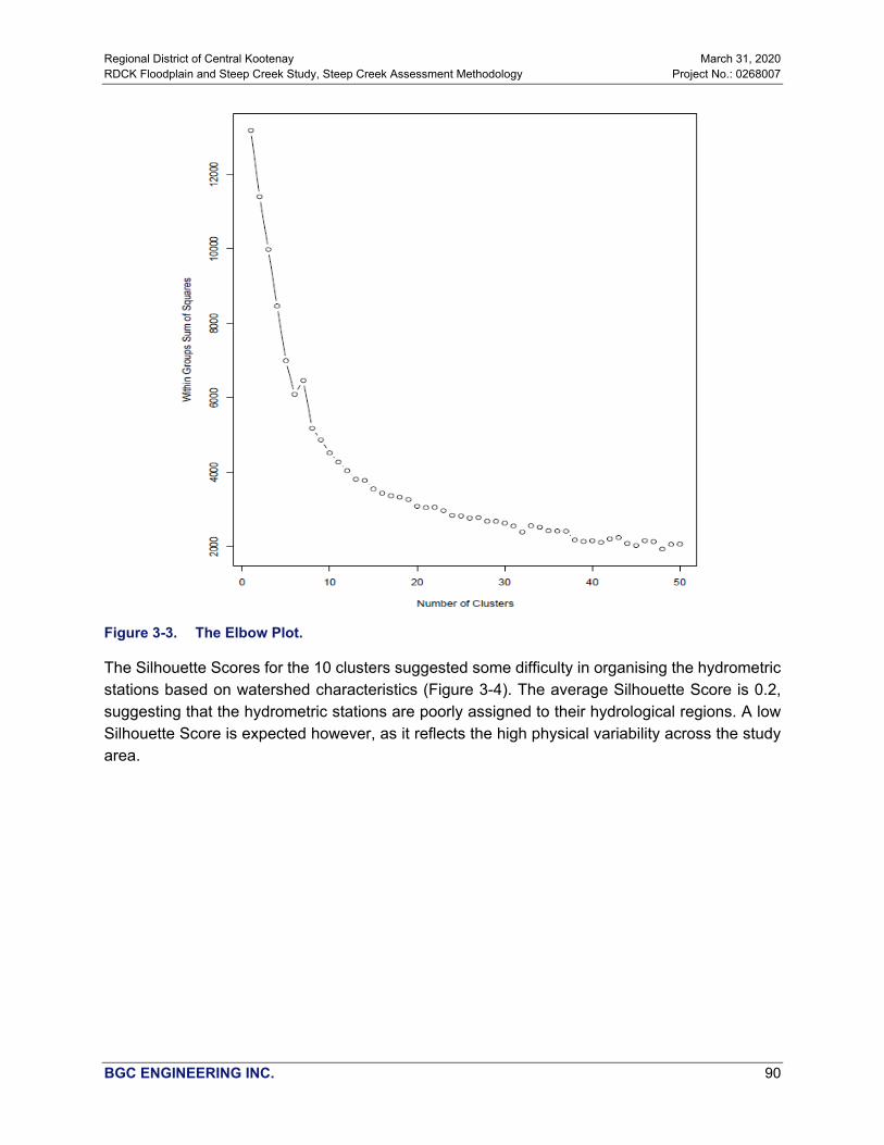
Regional District of Central Kootenay March 31, 2020 RDCK Floodplain and Steep Creek Study, Steep Creek Assessment Methodology Project No.: 0268007
BGC ENGINEERING INC. 90
Figure 3-3. The Elbow Plot.
The Silhouette Scores for the 10 clusters suggested some difficulty in organising the hydrometric stations based on watershed characteristics (Figure 3-4). The average Silhouette Score is 0.2, suggesting that the hydrometric stations are poorly assigned to their hydrological regions. A low Silhouette Score is expected however, as it reflects the high physical variability across the study area.

Regional District of Central Kootenay March 31, 2020 RDCK Floodplain and Steep Creek Study, Steep Creek Assessment Methodology Project No.: 0268007
BGC ENGINEERING INC. 91
Figure 3-4. Silhouette score.
The organization of the hydrometric stations into clusters is compiled in a dendrogram (Figure 3-5). The y-axis is the dissimilarity index based on the distance metric. The horizontal axis represents the Ward’s Distance (d). The green boxes separate the clusters. The 10 clusters are shown along the bottom of the dendrogram. Because we do not know how many clusters there should be in the landscape, the merging process was stopped once the clusters were more dissimilar than a threshold of approximately 90. The threshold was selected to generate a number of clusters consistent with the Elbow Plot.

Regional District of Central Kootenay March 31, 2020 RDCK Floodplain and Steep Creek Study, Steep Creek Assessment Methodology Project No.: 0268007
BGC ENGINEERING INC. 92
Figure 3-5. Dendrogram.

Regional District of Central Kootenay March 31, 2020 RDCK Floodplain and Steep Creek Study, Steep Creek Assessment Methodology Project No.: 0268007
BGC ENGINEERING INC. 93
3.5.2.1. Physical Basis of Regions and Flood Characteristics
The spatial distribution of the clusters is considered physically plausible, considering the range in the climate watershed characteristics. Significant regional variations are expected due to the influence of the mountain ranges across the study area (e.g., Coast Mountains, Monashees, the Columbia Trench, and the Rocky Mountains). These orographic effects are expected to control, at least in part, the distribution clusters (Figure 3-6).
Figure 3-6. Spatial distribution of 10 clusters.
Regional District of Central Kootenay March 31, 2020 RDCK Floodplain and Steep Creek Study, Steep Creek Assessment Methodology Project No.: 0268007
BGC ENGINEERING INC. 94
The clusters that cover the RDCK region include 1 (blue), 4 (red), and 7 (lilac) with 188, 154, and 158 hydrometric stations, respectively. Cluster 1 is defined by the influence of the Rocky Mountains to the east forming the physiographic boundary with Alberta. Most flood events in this cluster are caused by snowmelt or rain-on-snow events in the spring. The eastern range of the Coastal mountains to the west also includes a small group of hydrometric station assigned to Cluster 1. Cluster 4 is defined generally by a climate characteristic of the semi-arid plateau between major mountain ranges. Most flood events are snowmelt dominated in the spring. In this drier climate, evaporation from water surfaces and from the land as well as transpiration from vegetation make up a large component of the regional water balance. Additional hydrometric stations assigned to Cluster 4 are in the montane cordillera to the east where flood events are often associated with rain-on-snow events during the spring freshet. Cluster 7 is defined by the southern edge of the Rocky Mountains in northwestern Montana. Significant floods in this region are caused by runoff from rain associated with moist air masses from the Gulf of Mexico, although most annual peak discharge events are from snowmelt or rain-on-snow events in the spring.
3.5.2.2. Manual Adjustments
The clusters were further separated manually due to the large number of hydrometric stations in each cluster. Cluster 1 was separated into the eastern and western ranges of the Rocky Mountains. The small group of hydrometric stations located along the eastern range of the Coastal Mountains were also separated from Cluster 1. Cluster 4 was separated into the eastern portion in the montane cordillera and the western portion in the semi-arid plateau. Cluster 7 was not separated due to the limited geographic spread of the hydrometric stations. Based on these manual adjustments, Cluster 1 West, 4 East, and 7 cover the RDCK region (Figure 3-7).

Regional District of Central Kootenay March 31, 2020 RDCK Floodplain and Steep Creek Study, Steep Creek Assessment Methodology Project No.: 0268007
BGC ENGINEERING INC. 95
Figure 3-7. Clusters that cover the RDCK region.
The clusters were further separated based on the scale of watershed area. The coefficient of variation (CV) is required to be constant for a given homogeneous region. A relationship between the watershed area and L-CV is observed in the clusters that cover the RDCK. However, the strength of the relationship varies considerably (Table 3-11). In a flood regionalization study in British Columbia, Wang (2000) observed that in L-moment space, the L-CV varied with watershed area for the defined clusters making them heterogeneous. Wang (2000) demonstrated that the small watersheds show an increase and the large watersheds show a decrease in the L-CV.

Regional District of Central Kootenay March 31, 2020 RDCK Floodplain and Steep Creek Study, Steep Creek Assessment Methodology Project No.: 0268007
BGC ENGINEERING INC. 96
Table 3-11. R2 for regression between watershed area and L-CV
Cluster Number of Hydrometric Stations
R2 for regression between watershed area and L-CV
1 West 88 0.01
4 East 45 0.12
7 158 0.15
To account for the lack of constancy in the L-CV reported by Wang (2000) and observed in the clusters, the range in the watershed area considered in the study was modified to include two groups: 1) less than 500 km2 and 2) more than 500 km2 up to 5,000 km2. The clusters that cover the RDCK region thus include the following which will be the focus of the results herein.
• Cluster 1 West < 500 km2 • Cluster 1 West > 500 km2 • Cluster 4 West < 500 km2 • Cluster 4 West > 500 km2 • Cluster 7 < 500 km2 • Cluster 7 > 500 km2
3.5.2.3. Refinement of the Hydrometric Station Selection
The final number of hydrometric stations, including the range of discordancy (Di) values, for each hydrologic region is presented in Table 3-12. The number of hydrometric stations removed is based on the criteria presented in Section 3.4.2.4.
Table 3-12. Final number of hydrometric stations and range in discordancy measure for each hydrologic region.
Cluster Watershed
Area Range
Initial Number of
Hydrometric Stations
Number of Hydrometric
Stations Removed
Final Number of
Hydrometric Stations
Di (Min)
Di (Max)
Di (Mean)
1 West < 500 km2 36 10 26 0.13 3.0 1
> 500 km2 52 28 24 0.09 3.0 1
4 East < 500 km2 43 9 34 0.04 2.8 1
> 500 km2 2 Not enough data for regionalization
7 < 500 km2 75 35 40 0.09 2.6 1
> 500 km2 83 65 18 0.11 2.9 1
3.5.2.4. Homogeneity
The H-Test results are summarized in Table 3-13. A cluster is declared heterogeneous if H is sufficiently “large”. Hosking and Wallis (1997) recommend a cluster be considered “definitely heterogeneous” if H > 2. Increasing the threshold implies that more heterogeneous regions are
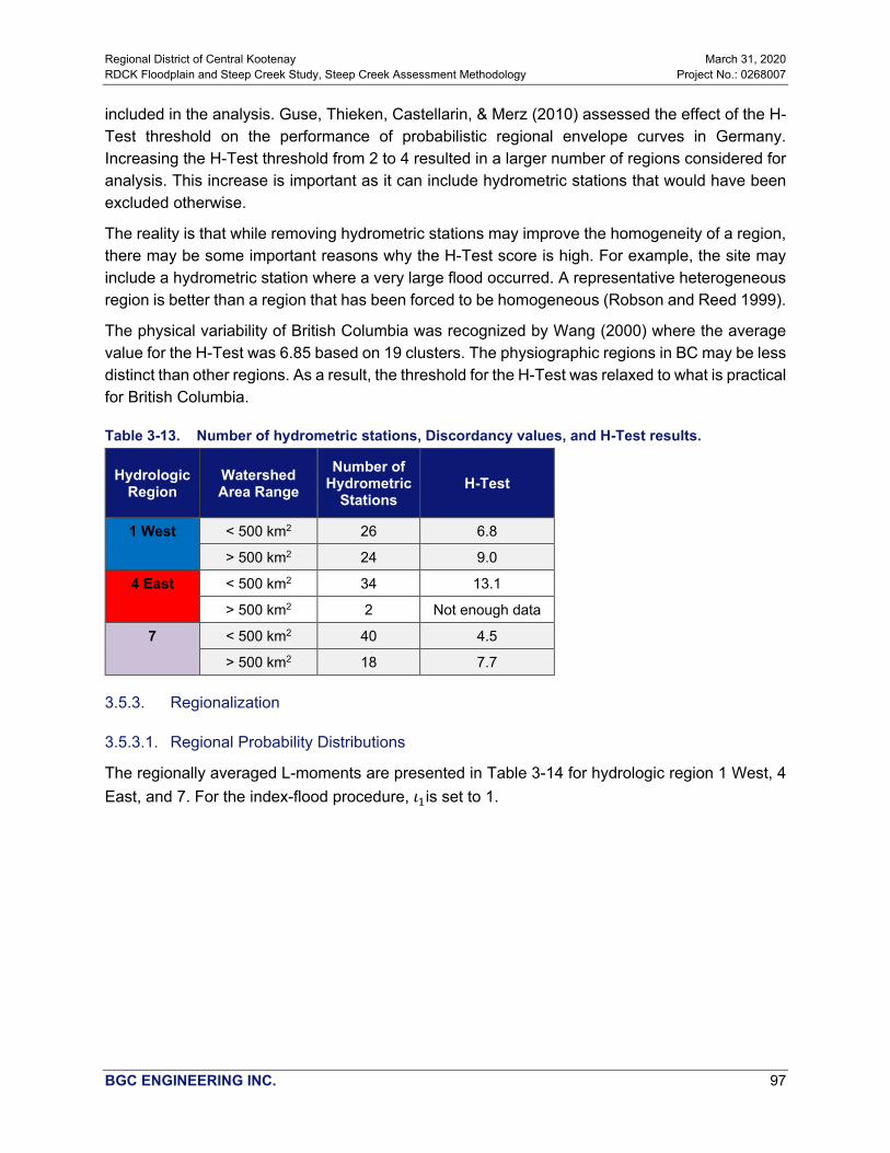
Regional District of Central Kootenay March 31, 2020 RDCK Floodplain and Steep Creek Study, Steep Creek Assessment Methodology Project No.: 0268007
BGC ENGINEERING INC. 97
included in the analysis. Guse, Thieken, Castellarin, & Merz (2010) assessed the effect of the H-Test threshold on the performance of probabilistic regional envelope curves in Germany. Increasing the H-Test threshold from 2 to 4 resulted in a larger number of regions considered for analysis. This increase is important as it can include hydrometric stations that would have been excluded otherwise.
The reality is that while removing hydrometric stations may improve the homogeneity of a region, there may be some important reasons why the H-Test score is high. For example, the site may include a hydrometric station where a very large flood occurred. A representative heterogeneous region is better than a region that has been forced to be homogeneous (Robson and Reed 1999).
The physical variability of British Columbia was recognized by Wang (2000) where the average value for the H-Test was 6.85 based on 19 clusters. The physiographic regions in BC may be less distinct than other regions. As a result, the threshold for the H-Test was relaxed to what is practical for British Columbia.
Table 3-13. Number of hydrometric stations, Discordancy values, and H-Test results.
Hydrologic Region
Watershed Area Range
Number of Hydrometric
Stations H-Test
1 West < 500 km2 26 6.8
> 500 km2 24 9.0
4 East < 500 km2 34 13.1
> 500 km2 2 Not enough data
7 < 500 km2 40 4.5
> 500 km2 18 7.7
3.5.3. Regionalization
3.5.3.1. Regional Probability Distributions
The regionally averaged L-moments are presented in Table 3-14 for hydrologic region 1 West, 4 East, and 7. For the index-flood procedure, 𝜄𝜄1is set to 1.
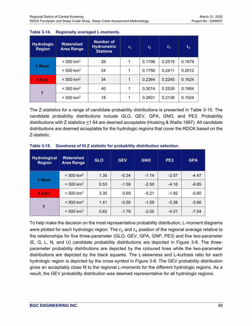
Regional District of Central Kootenay March 31, 2020 RDCK Floodplain and Steep Creek Study, Steep Creek Assessment Methodology Project No.: 0268007
BGC ENGINEERING INC. 98
Table 3-14. Regionally averaged L-moments.
Hydrologic Region
Watershed Area Range
Number of Hydrometric
Stations 𝜾𝜾𝟏𝟏 𝜾𝜾𝟐𝟐 𝒕𝒕𝟑𝟑 𝒕𝒕𝟒𝟒
1 West < 500 km2 26 1 0.1796 0.2519 0.1879
> 500 km2 24 1 0.1756 0.2411 0.2012
4 East < 500 km2 34 1 0.2364 0.2245 0.1624
7 < 500 km2 40 1 0.3014 0.2539 0.1904
> 500 km2 18 1 0.2601 0.2138 0.1924
The Z-statistics for a range of candidate probability distributions is presented in Table 3-15. The candidate probability distributions include GLO, GEV, GPA, GNO, and PE3. Probability distributions with Z statistics <1.64 are deemed acceptable (Hosking & Wallis 1997). All candidate distributions are deemed acceptable for the hydrologic regions that cover the RDCK based on the Z-statistic.
Table 3-15. Goodness of fit Z statistic for probability distribution selection.
Hydrological Region
Watershed Area Range GLO GEV GNO PE3 GPA
1 West < 500 km2 1.30 -0.34 -1.14 -2.57 -4.47
> 500 km2 0.53 -1.59 -2.50 -4.16 -6.85
4 East < 500 km2 3.30 0.69 -0.21 -1.92 -5.60
7 < 500 km2 1.41 -0.59 -1.59 -3.38 -5.66
> 500 km2 0.62 -1.79 -2.55 -4.01 -7.54
To help make the decision on the most representative probability distribution, L-moment diagrams were plotted for each hydrologic region. The 𝑡𝑡3 and 𝑡𝑡4 position of the regional average relative to the relationships for five three-parameter (GLO, GEV, GPA, GNP, PE3) and five two-parameter (E, G, L, N, and U) candidate probability distributions are depicted in Figure 3-8. The three-parameter probability distributions are depicted by the coloured lines while the two-parameter distributions are depicted by the black squares. The L-skewness and L-kurtosis ratio for each hydrologic region is depicted by the cross symbol in Figure 3-8. The GEV probability distribution gives an acceptably close fit to the regional L-moments for the different hydrologic regions. As a result, the GEV probability distribution was deemed representative for all hydrologic regions.

Regional District of Central Kootenay March 31, 2020 RDCK Floodplain and Steep Creek Study, Steep Creek Assessment Methodology Project No.: 0268007
BGC ENGINEERING INC. 99
Figure 3-8. L-moment ratio diagram for each hydrologic region.

Regional District of Central Kootenay March 31, 2020 RDCK Floodplain and Steep Creek Study, Steep Creek Assessment Methodology Project No.: 0268007
BGC ENGINEERING INC. 100
3.5.3.2. Parameter Estimation
The regionally weighted L-moments are used to estimate the parameters of the GEV probability distribution. The parameters for each hydrologic region are presented in Table 3-16.
Table 3-16. Parameter estimates for the GEV distribution.
Hydrological Region
Watershed Area limit 𝝃𝝃 𝜶𝜶 𝜿𝜿
1 West < 500 km2 0.8369 0.2280 -0.1236
> 500 km2 0.8421 0.2269 -0.1078
4 East < 500 km2 0.7908 0.3139 -0.0832
7 < 500 km2 0.7257 0.3814 -0.1266
> 500 km2 0.7724 0.3513 -0.0671
3.5.3.3. Growth Curves and Error Bounds
The regional growth curves and error bounds are presented for each hydrologic region in Figure 3-9.

Regional District of Central Kootenay March 31, 2020 RDCK Floodplain and Steep Creek Study, Steep Creek Assessment Methodology Project No.: 0268007
BGC ENGINEERING INC. 101
Figure 3-9. Growth curves for each hydrologic region.
3.5.3.4. Index Flood
The regional equations for the index-flood for each hydrologic region are presented in Table 3-17. The provincial equations are also included at the end of Table 3-17. The results are reported to 5 significant figures. However, a total of 5 equations are developed for each hydrologic region and across the province with the intention to average the index-flood estimates. Consequently, the results should be rounded to the nearest unit for flood magnitudes greater than 10 m3/s. The adjusted R2 is included for comparison of the models. Models with more watershed characteristics tend to have a lower adjusted R2 as these models are penalized for increased number of independent variables.

Regional District of Central Kootenay March 31, 2020 RDCK Floodplain and Steep Creek Study, Steep Creek Assessment Methodology Project No.: 0268007
BGC ENGINEERING INC. 102
Table 3-17. Regional and provincial equations for the index-flood including the adjusted R2.
Hydrologic Region
Watershed Area
Range Index-flood Equations Adj.
R2
1 West < 500 km2
42 to 454 km2
1 log𝑄𝑄𝑚𝑚 = −0.26675 + 1.8591(log𝐴𝐴𝐴𝐴𝐴𝐴𝑎𝑎) − 0.011874(𝑆𝑆𝑆𝑆𝑆𝑆𝑆𝑆𝐴𝐴) − 0.00035620 (𝐶𝐶𝐴𝐴𝑛𝑛_𝐸𝐸𝑆𝑆𝐴𝐴𝑣𝑣)+ 0.0017297(𝑃𝑃𝐴𝐴𝑆𝑆) 0.88
2 log𝑄𝑄𝑚𝑚 = −2.0342 + 1.9445(log𝐴𝐴𝐴𝐴𝐴𝐴𝑎𝑎) − 0.0067267(𝑆𝑆𝑆𝑆𝑆𝑆𝑆𝑆𝐴𝐴) + 0.0014489(𝑆𝑆𝐴𝐴𝑃𝑃) 0.89
3 log𝑄𝑄𝑚𝑚 = −0.10229 + 1.8039(log𝐴𝐴𝐴𝐴𝐴𝐴𝑎𝑎) − 0.012794(𝑆𝑆𝑆𝑆𝑆𝑆𝑆𝑆𝐴𝐴) − 0.00037750(𝐶𝐶𝐴𝐴𝑛𝑛_𝐸𝐸𝑆𝑆𝐴𝐴𝑣𝑣)+ 0.0017281(𝑃𝑃𝐴𝐴𝑆𝑆) + 0.40159(𝑊𝑊𝑎𝑎𝑡𝑡𝐴𝐴𝐴𝐴_𝑊𝑊𝐴𝐴𝑡𝑡𝑆𝑆𝑎𝑎𝑛𝑛𝑑𝑑) 0.90
4 log𝑄𝑄𝑚𝑚 = 1.3990 + 1.9139(log𝐴𝐴𝐴𝐴𝐴𝐴𝑎𝑎) − 0.012626(𝑆𝑆𝑆𝑆𝑆𝑆𝑆𝑆𝐴𝐴) − 0.00030660(𝐶𝐶𝐴𝐴𝑛𝑛_𝐸𝐸𝑆𝑆𝐴𝐴𝑣𝑣) + 0.0016306(𝑃𝑃𝐴𝐴𝑆𝑆)+ 0.46153(𝑊𝑊𝑎𝑎𝑡𝑡𝐴𝐴𝐴𝐴𝑊𝑊𝑊𝑊𝑊𝑊𝑊𝑊𝑏𝑏𝑛𝑛𝑊𝑊) − 0.025646(𝐶𝐶𝑁𝑁) 0.90
5 log𝑄𝑄𝑚𝑚 = 19.653 + 0.0012794(𝑅𝑅𝐴𝐴𝑆𝑆𝑅𝑅𝐴𝐴𝑅𝑅) − 0.027375(𝑆𝑆𝑆𝑆𝑆𝑆𝑆𝑆𝐴𝐴) + 0.33879(𝐶𝐶𝐴𝐴𝑛𝑛_𝐿𝐿𝑎𝑎𝑡𝑡)+ 0.2423219(𝐶𝐶𝐴𝐴𝑛𝑛_𝐿𝐿𝑆𝑆𝑛𝑛𝐿𝐿) − 0.00062330(𝐶𝐶𝐴𝐴𝑛𝑛_𝐸𝐸𝑆𝑆𝐴𝐴𝑣𝑣) + 0.0011831(𝑃𝑃𝐴𝐴𝑆𝑆)− 0.064919(𝐶𝐶𝑁𝑁)
0.91
1 West > 500 km2
586 to 4312 km2
1 log𝑄𝑄𝑚𝑚 = −2.5781 + 2.0480(log𝐴𝐴𝐴𝐴𝐴𝐴𝑎𝑎) + 0.0012740 (𝑆𝑆𝐴𝐴𝑃𝑃) 0.83
2 log𝑄𝑄𝑚𝑚 = −2.3716 + 1.8939(log𝐴𝐴𝐴𝐴𝐴𝐴𝑎𝑎) + 0.41806(log𝐶𝐶𝑎𝑎𝑡𝑡𝑐𝑐ℎ_𝐿𝐿𝐴𝐴𝑛𝑛𝐿𝐿𝑡𝑡ℎ) + 0.0012775(𝑆𝑆𝐴𝐴𝑃𝑃) 0.82
3 log𝑄𝑄𝑚𝑚 = 1.3411 + 1.9306(log𝐴𝐴𝐴𝐴𝐴𝐴𝑎𝑎) + 0.18827(log𝐶𝐶𝑎𝑎𝑡𝑡𝑐𝑐ℎ_𝐿𝐿𝐴𝐴𝑛𝑛𝐿𝐿𝑡𝑡ℎ) + 0.0011046 (𝑆𝑆𝐴𝐴𝑃𝑃)− 0.04866(𝐶𝐶𝑁𝑁) 0.82
4 log𝑄𝑄𝑚𝑚 = −0.70946 + 1.6015(log𝐴𝐴𝐴𝐴𝐴𝐴𝑎𝑎) − 0.0081664(𝑆𝑆𝑆𝑆𝑆𝑆𝑆𝑆𝐴𝐴) + 0.0013574 (𝑆𝑆𝐴𝐴𝑃𝑃) + 0.057906 (𝑆𝑆𝐴𝐴𝑇𝑇)− 0.0036032(𝐼𝐼𝑆𝑆𝐴𝐴𝐴𝐴𝐹𝐹𝑡𝑡) 0.83
5 log𝑄𝑄𝑚𝑚 = 0.40059 + 1.6514(log𝐴𝐴𝐴𝐴𝐴𝐴𝑎𝑎) − 0.0082135(𝑆𝑆𝑆𝑆𝑆𝑆𝑆𝑆𝐴𝐴) + 0.0010135 (𝑆𝑆𝐴𝐴𝑃𝑃) + 0.15045 (𝑆𝑆𝐴𝐴𝑇𝑇)− 0.016425(𝐼𝐼𝑆𝑆𝐴𝐴𝐴𝐴𝐹𝐹𝑡𝑡) − 0.19361(𝑊𝑊𝑎𝑎𝑡𝑡𝐴𝐴𝐴𝐴_𝑊𝑊𝐴𝐴𝑡𝑡𝑆𝑆𝑎𝑎𝑛𝑛𝑑𝑑) 0.88
4 East < 500 km2
6 to 441 km2
1 log𝑄𝑄𝑚𝑚 = −4.0074 + 2.7378(log𝐴𝐴𝐴𝐴𝐴𝐴𝑎𝑎) + 0.0022206 (𝑃𝑃𝐴𝐴𝑆𝑆) 0.94

Regional District of Central Kootenay March 31, 2020 RDCK Floodplain and Steep Creek Study, Steep Creek Assessment Methodology Project No.: 0268007
BGC ENGINEERING INC. 103
Hydrologic Region
Watershed Area
Range Index-flood Equations Adj.
R2
2 log𝑄𝑄𝑚𝑚 = −2.6565 + 2.6835(log𝐴𝐴𝐴𝐴𝐴𝐴𝑎𝑎) + 0.0020715 (𝑃𝑃𝐴𝐴𝑆𝑆) − 0.017655(𝐶𝐶𝑁𝑁) 0.94
3 log𝑄𝑄𝑚𝑚 = −2.0471 + 2.6959(log𝐴𝐴𝐴𝐴𝐴𝐴𝑎𝑎) + 0.0019774 (𝑃𝑃𝐴𝐴𝑆𝑆) − 0.28299(𝑊𝑊𝑎𝑎𝑡𝑡𝐴𝐴𝐴𝐴_𝑊𝑊𝐴𝐴𝑡𝑡𝑆𝑆𝑎𝑎𝑛𝑛𝑑𝑑)− 0.025781(𝐶𝐶𝑁𝑁) 0.95
4 log𝑄𝑄𝑚𝑚 = −2.5027 + 2.8400(log𝐴𝐴𝐴𝐴𝐴𝐴𝑎𝑎) + 0.0012339(𝑆𝑆𝑆𝑆𝑆𝑆𝑆𝑆𝐴𝐴) + 0.0019861 (𝑃𝑃𝐴𝐴𝑆𝑆)− 0.28224(𝑊𝑊𝑎𝑎𝑡𝑡𝐴𝐴𝐴𝐴_𝑊𝑊𝐴𝐴𝑡𝑡𝑆𝑆𝑎𝑎𝑛𝑛𝑑𝑑) − 0.025382(𝐶𝐶𝑁𝑁) 0.96
5 log𝑄𝑄𝑚𝑚 = −1.5104 + 2.7686(log𝐴𝐴𝐴𝐴𝐴𝐴𝑎𝑎) + 0.0011343(𝑆𝑆𝑆𝑆𝑆𝑆𝑆𝑆𝐴𝐴) + 0.0018268 (𝑃𝑃𝐴𝐴𝑆𝑆) − 0.0069562(𝐼𝐼𝑆𝑆𝐴𝐴𝐴𝐴𝐹𝐹𝑡𝑡)− 0.29068(𝑊𝑊𝑎𝑎𝑡𝑡𝐴𝐴𝐴𝐴_𝑊𝑊𝐴𝐴𝑡𝑡𝑆𝑆𝑎𝑎𝑛𝑛𝑑𝑑) − 0.027162(𝐶𝐶𝑁𝑁) 0.95
7 < 500 km2 8 to 471 km2
1 log𝑄𝑄𝑚𝑚 = −3.8856 + 1.8844(log𝐴𝐴𝐴𝐴𝐴𝐴𝑎𝑎) + 0.010435�𝑃𝑃𝑃𝑃𝑇𝑇𝑁𝑁𝑊𝑊� 0.74
2 log𝑄𝑄𝑚𝑚 = −3.9002 + 1.9484(log𝐴𝐴𝐴𝐴𝐴𝐴𝑎𝑎) + 0.10058�𝑃𝑃𝑃𝑃𝑇𝑇𝑁𝑁𝑊𝑊� − 0.17007(𝑊𝑊𝑎𝑎𝑡𝑡𝐴𝐴𝐴𝐴_𝑊𝑊𝐴𝐴𝑡𝑡𝑆𝑆𝑎𝑎𝑛𝑛𝑑𝑑) 0.74
3 log𝑄𝑄𝑚𝑚 = −4.4499 + 2.0486(log𝐴𝐴𝐴𝐴𝐴𝐴𝑎𝑎) + 0.0051660(𝑃𝑃𝑃𝑃𝑇𝑇𝑁𝑁𝑊𝑊) + 0.0062765(𝑃𝑃𝑃𝑃𝑇𝑇𝑠𝑠𝑚𝑚)− 0.21014(𝑊𝑊𝑎𝑎𝑡𝑡𝐴𝐴𝐴𝐴_𝑊𝑊𝐴𝐴𝑡𝑡𝑆𝑆𝑎𝑎𝑛𝑛𝑑𝑑) 0.74
4 log𝑄𝑄𝑚𝑚 = −20.730 + 1.7210(log𝐴𝐴𝐴𝐴𝐴𝐴𝑎𝑎) + 0.36720(𝐶𝐶𝐴𝐴𝑛𝑛_𝐿𝐿𝑎𝑎𝑡𝑡) − 0.00093400(𝐶𝐶𝐴𝐴𝑛𝑛𝐸𝐸𝑊𝑊𝑊𝑊𝐸𝐸)+ 0.13920�𝑃𝑃𝑃𝑃𝑇𝑇𝑠𝑠𝑁𝑁� − 0.30900(𝑊𝑊𝑎𝑎𝑡𝑡𝐴𝐴𝐴𝐴_𝑊𝑊𝐴𝐴𝑡𝑡𝑆𝑆𝑎𝑎𝑛𝑛𝑑𝑑) 0.75
5 log𝑄𝑄𝑚𝑚 = −1.9967 + 2.9199(log𝐴𝐴𝐴𝐴𝐴𝐴𝑎𝑎) − 0.44581(log𝐶𝐶𝑎𝑎𝑡𝑡𝑐𝑐ℎ 𝐿𝐿𝐴𝐴𝑛𝑛𝐿𝐿𝑡𝑡ℎ) + 0.22219(𝐶𝐶𝐴𝐴𝑛𝑛_𝐿𝐿𝑎𝑎𝑡𝑡)+ 0.11838(𝐶𝐶𝐴𝐴𝑛𝑛_𝐿𝐿𝑆𝑆𝑛𝑛𝐿𝐿) + 0.007305(𝑃𝑃𝑃𝑃𝑇𝑇𝑁𝑁𝑊𝑊) − 0.32687(𝑊𝑊𝑎𝑎𝑡𝑡𝐴𝐴𝐴𝐴_𝑊𝑊𝐴𝐴𝑡𝑡𝑆𝑆𝑎𝑎𝑛𝑛𝑑𝑑) 0.75
7 >500 km2 529 to 4138 km2
1 log𝑄𝑄𝑚𝑚 = −2.8251 + 2.0765(log𝐴𝐴𝐴𝐴𝐴𝐴𝑎𝑎) − 0.65058(𝑆𝑆𝐴𝐴𝑇𝑇) − 0.01087(𝑃𝑃𝐴𝐴𝑆𝑆) + 0.15245(𝑃𝑃𝑃𝑃𝑇𝑇𝑁𝑁𝑊𝑊)+ 0.014215(𝑃𝑃𝑃𝑃𝑇𝑇𝑠𝑠𝑚𝑚) + 0.14232(𝐼𝐼𝑆𝑆𝐴𝐴𝐴𝐴𝐹𝐹𝑡𝑡) 0.93
2 log𝑄𝑄𝑚𝑚 = 0.51542 + 1.4852(log𝐴𝐴𝐴𝐴𝐴𝐴𝑎𝑎) − 0.024121(𝑆𝑆𝑆𝑆𝑆𝑆𝑆𝑆𝐴𝐴) − 0.0078710(𝑆𝑆𝐴𝐴𝑃𝑃) − 0.69867(𝑆𝑆𝐴𝐴𝑇𝑇)− 0.010055(𝑃𝑃𝐴𝐴𝑆𝑆) 0.93
3 log𝑄𝑄𝑚𝑚 = −0.28887 + 2.1311(log𝐴𝐴𝐴𝐴𝐴𝐴𝑎𝑎) − 0.00048080(𝐶𝐶𝐴𝐴𝑛𝑛_𝐸𝐸𝑆𝑆𝐴𝐴𝑣𝑣) − 0.59076(𝑆𝑆𝐴𝐴𝑇𝑇) − 0.10256(𝑃𝑃𝐴𝐴𝑆𝑆)+ 0.14034(𝑃𝑃𝑃𝑃𝑇𝑇𝑁𝑁𝑊𝑊) + 0.14291(𝑃𝑃𝑃𝑃𝑇𝑇𝑠𝑠𝑚𝑚) + 0.018084(𝐼𝐼𝑆𝑆𝐴𝐴𝐴𝐴𝐹𝐹𝑡𝑡) 0.94

Regional District of Central Kootenay March 31, 2020 RDCK Floodplain and Steep Creek Study, Steep Creek Assessment Methodology Project No.: 0268007
BGC ENGINEERING INC. 104
Hydrologic Region
Watershed Area
Range Index-flood Equations Adj.
R2
4 log𝑄𝑄𝑚𝑚 = −12.290 + 4.2860(log𝐴𝐴𝐴𝐴𝐴𝐴𝑎𝑎) − 4.4640(log𝐶𝐶𝑎𝑎𝑡𝑡𝑐𝑐ℎ_𝐿𝐿𝐴𝐴𝑛𝑛𝐿𝐿𝑡𝑡ℎ) + 0.54240(𝐶𝐶𝐴𝐴𝑛𝑛_𝐿𝐿𝑎𝑎𝑡𝑡)+ 0.19690(𝐶𝐶𝐴𝐴𝑛𝑛_𝐿𝐿𝑆𝑆𝑛𝑛𝐿𝐿) − 0.0066490(𝑃𝑃𝐴𝐴𝑆𝑆) + 0.013790(𝑃𝑃𝑃𝑃𝑇𝑇𝑁𝑁𝑊𝑊) + 0.38640(𝐼𝐼𝑆𝑆𝐴𝐴𝐴𝐴𝐹𝐹𝑡𝑡) 0.94
5 log𝑄𝑄𝑚𝑚 = −6.0632 + 2.1265(log𝐴𝐴𝐴𝐴𝐴𝐴𝑎𝑎) + 0.0053923(𝑃𝑃𝑃𝑃𝑇𝑇𝑁𝑁𝑊𝑊) + 0.030556(𝐼𝐼𝑆𝑆𝐴𝐴𝐴𝐴𝐹𝐹𝑡𝑡) 0.90
Provincial Model
1 to 4,888 km2
1 log𝑄𝑄𝑚𝑚 = −3.6850 + 2.0590(log𝐴𝐴𝐴𝐴𝐴𝐴𝑎𝑎) + 0.0011270(𝑆𝑆𝐴𝐴𝑃𝑃) + 0.00038470(𝑃𝑃𝐴𝐴𝑆𝑆)− 0.066740(𝑊𝑊𝑎𝑎𝑡𝑡𝐴𝐴𝐴𝐴_𝑊𝑊𝐴𝐴𝑡𝑡𝑆𝑆𝑎𝑎𝑛𝑛𝑑𝑑) + 0.012860(𝐶𝐶𝑁𝑁) 0.88
2 log𝑄𝑄𝑚𝑚 = −3.5600 + 2.0340(log𝐴𝐴𝐴𝐴𝐴𝐴𝑎𝑎) + 0.0011100(𝑆𝑆𝐴𝐴𝑃𝑃) + 0.00038230(𝑃𝑃𝐴𝐴𝑆𝑆) + 0.011550(𝐶𝐶𝑁𝑁) 0.88 3 log𝑄𝑄𝑚𝑚 = −6.1210 + 2.0630(log𝐴𝐴𝐴𝐴𝐴𝐴𝑎𝑎) − 0.019620(𝐶𝐶𝐴𝐴𝑛𝑛_𝐿𝐿𝑆𝑆𝑛𝑛𝐿𝐿) + 0.0010960(𝑆𝑆𝐴𝐴𝑃𝑃)
+ 0.00041080(𝑃𝑃𝐴𝐴𝑆𝑆) − 0.074170(𝑊𝑊𝑎𝑎𝑡𝑡𝐴𝐴𝐴𝐴_𝑊𝑊𝐴𝐴𝑡𝑡𝑆𝑆𝑎𝑎𝑛𝑛𝑑𝑑) + 0.014570(𝐶𝐶𝑁𝑁) 0.88
4 log𝑄𝑄𝑚𝑚 = −3.3270 + 2.0570(log𝐴𝐴𝐴𝐴𝐴𝐴𝑎𝑎) − 0.00018960(𝐶𝐶𝐴𝐴𝑛𝑛_𝐸𝐸𝑆𝑆𝐴𝐴𝑣𝑣) + 0.0011270(𝑆𝑆𝐴𝐴𝑃𝑃)− 0.030000(𝑆𝑆𝐴𝐴𝑇𝑇) + 0.00034200(𝑃𝑃𝐴𝐴𝑆𝑆) − 0.074200(𝑊𝑊𝑎𝑎𝑡𝑡𝐴𝐴𝐴𝐴_𝑊𝑊𝐴𝐴𝑡𝑡𝑆𝑆𝑎𝑎𝑛𝑛𝑑𝑑)+ 0.013040(𝐶𝐶𝑁𝑁)
0.88
5 log𝑄𝑄𝑚𝑚 = −2.6520 + 2.0190(log𝐴𝐴𝐴𝐴𝐴𝐴𝑎𝑎) + 0.0010620(𝑆𝑆𝐴𝐴𝑃𝑃) + 0.00034010(𝑃𝑃𝐴𝐴𝑆𝑆)− 0.074200(𝑊𝑊𝑎𝑎𝑡𝑡𝐴𝐴𝐴𝐴_𝑊𝑊𝐴𝐴𝑡𝑡𝑆𝑆𝑎𝑎𝑛𝑛𝑑𝑑) + 0.013040(𝐶𝐶𝑁𝑁) 0.87

Regional District of Central Kootenay March 31, 2020 RDCK Floodplain and Steep Creek Study, Steep Creek Assessment Methodology Project No.: 0268007
BGC ENGINEERING INC. 105
3.5.4. Error Statistics
The weighted standardized error statistics for the regional and provincial model over a range of peak discharges for the different hydrologic regions are presented in Table 3-18. The error statistics are not consistent across all hydrologic regions. The regional model may be selected for the 4 East < 500 km2 hydrologic region. In the case of the 1 West region, either the regional or provincial model would be considered adequate. Lastly, the regional model is probably the model of choice for the 7 hydrologic regions. As expected, the error statistics for the lower peak discharges are lower than those for higher peak discharges reflecting the increased uncertainty in higher quantile estimates.

Regional District of Central Kootenay March 31, 2020 RDCK Floodplain and Steep Creek Study, Steep Creek Assessment Methodology Project No.: 0268007
ENGINEERING INC. 106
Table 3-18. Weighted standardized error statistics for the regional and provincial models over a range of peak discharges. Green highlighted cells depict a positive bias while the red highlighted cells depict a negative bias.
Error Stats AEP 1 West < 500 km2 1 West > 500 km2 4 East < 500 km2 7 < 500 km2 7 > 500 km2
Regional Qm
Provincial Qm
Regional Qm
Provincial Qm
Regional Qm
Provincial Qm
Regional Qm
Provincial Qm
Regional Qm
Provincial Qm
SRMSE
0.5 0.23 0.32 0.27 0.26 0.53 1.10 2.71 3.80 0.19 0.99
0.1 0.28 0.32 0.26 0.28 0.35 0.76 3.08 4.10 0.21 0.96
0.02 0.40 0.42 0.31 0.33 0.36 0.67 3.70 4.80 0.27 1.01
0.005 0.54 0.54 0.38 0.39 0.41 0.67 4.37 5.59 0.36 1.09
SPercent Error
0.5 18 22 20 21 32 68 70 122 15 65
0.1 24 23 20 24 24 50 74 128 14 65
0.02 32 30 25 29 27 41 84 144 20 68
0.005 42 38 30 33 32 39 97 165 29 74
SBIAS
0.5 0.03 -0.04 0.04 -0.09 0.10 0.37 0.39 1.03 0.03 0.39
0.1 0.06 -0.02 0.04 -0.07 0.07 0.26 0.44 1.08 0.03 0.39
0.02 0.09 0.01 0.06 -0.06 0.07 0.22 0.52 1.21 0.04 0.42
0.005 0.13 0.06 0.08 -0.03 0.08 0.20 0.62 1.37 0.06 0.45

Regional District of Central Kootenay March 31, 2020 RDCK Floodplain and Steep Creek Study, Steep Creek Assessment Methodology Project No.: 0268007
BGC ENGINEERING INC. 107
3.6. Application to Ungauged Watersheds
The goal of the regionalization of floods is to estimate quantiles for ungauged watersheds in the RDCK. A total of 11 steep creek watersheds are modeled for clearwater floods. To begin, a watershed polygon was defined for each ungauged watershed, as shown in Figure 3-10. The suite of 18 watershed characteristics were then extracted and averaged over the area for each ungauged watershed. The resulting watershed characteristics are presented in Table 3-19.
The ungauged watersheds were subsequently assigned to one of the hydrologic regions identified across the study area. The hydrologic region assignment was completed using the Random Forest classification algorithm. Once the ungauged watershed was assigned to a hydrologic region; the index-flood was estimated based on the appropriate model (regional and / or provincial). The peak discharges were then estimated for a range of AEPs using the index-flood estimate and the appropriate regional growth curve. The hydrologic region assignment, index-flood estimate, and peak discharges for each ungauged watershed are presented in Table 3-20.
The magnitude of the peak discharges is influenced by the watershed characteristics. This is because the index-flood is calculated using a multiple linear regression that depends on the watershed characteristics that define the best 5 models for a given region. Two watersheds of similar area may have significantly different peak discharge estimates because of major differences in watershed characteristics. For example, Kokanee Creek and Eagle Creek share comparable watershed areas of 96 km2 and 99 km2, respectively. However, peak discharges for Kokanee Creek are approximately twice as much as than Eagle Creek, with the difference in magnitude attributed to difference in climate characteristics.

Regional District of Central Kootenay March 31, 2020 RDCK Floodplain and Steep Creek Study, Steep Creek Assessment Methodology Project No.: 0268007
BGC ENGINEERING INC. 108
Figure 3-10. Watershed polygons for the ungauged watersheds.
90 km

Regional District of Central Kootenay March 31, 2020 RDCK Floodplain and Steep Creek Study, Steep Creek Assessment Methodology Project No.: 0268007
BGC ENGINEERING INC. 109
Table 3-19. Watershed characteristics for the steep creek watersheds located in the RDCK.
Watershed Name Area (km2)
Relief (m)
Watershed Length
(km)
Slope (%)
Centroid Latitude
(degrees)
Centroid Longitude (degrees)
Centroid Elevation
(m) MAP (mm)
MAT (⁰C)
PAS (mm)
Forest (%)
Water and Wetland
(%) Urban
(%) CN
Eagle Creek 99.2 1686 1.7 101 49.833155 -118.282182 1357 946 2.8 469 94 0.0 0 68
Kuskonook Creek 4.5 1559 0.4 399 49.314555 -116.636917 1482 1176 3.1 612 31 0.0 0 64
Sitkum Creek 27.1 1612 0.9 170 49.644837 -117.221846 1487 1303 3.1 695 94 0.0 0 65
Redfish Creek 25.8 1614 1.0 155 49.661622 -117.071351 1508 1373 2.1 806 85 0.0 0 65
Harrop Creek 42.6 1639 1.4 120 49.54807 -117.040921 1408 1418 2.1 837 94 0.0 0 61
Procter Creek 7.6 1568 0.5 308 49.584417 -116.945682 1465 1290 2.6 718 80 9.0 0 61
Wilson Creek 560 2244 3.7 60 50.201776 -117.418123 1571 1400 2.1 823 70 0.4 0 67
Cooper Creek 244 2420 2.8 86 50.183916 -117.129217 2094 1477 1.3 931 68 0.1 0 70
Duhamel Creek 56.2 1616 1.5 105 49.632911 -117.273691 1486 1300 3.1 691 96 0.0 0 66
Kokanee Creek 96 2118 2.0 106 49.683629 -117.159364 1638 1405 2.0 839 67 0.0 0 64
Inonoaklin 392 1739 3.0 59 49.945716 -118.298492 1263 896 3.6 403 89 0.1 0 66

Regional District of Central Kootenay March 31, 2020 RDCK Floodplain and Steep Creek Study, Steep Creek Assessment Methodology Project No.: 0268007
BGC ENGINEERING INC. 110
Table 3-20. Hydrologic region assignment for the ungauged watersheds.
Watershed Hydrometric Station
Watershed Area (km2)
Hydrologic Region1
Qm (m3/s)
Peak Discharge (m3/s)
0.05 AEP
0.02 AEP
0.005 AEP
Eagle Creek - 99.2 4 East < 500 km2 13 12 23 36
Kuskonook Creek - 4.5 4 East < 500 km2 1.1 0.9 1.9 3.0
Sitkum Creek - 27.1 4 East < 500 km2 6 5.6 12 18
Redfish Creek 08NJ061 25.8 4 East < 500 km2 - 9 14 18
Harrop Creek - 42.6 4 East < 500 km2 11 10 20 31
Procter Creek - 7.6 4 East < 500 km2 2.0 1.8 3.7 5.7
Wilson Creek - 560 1 West > 500 km2 139 128 227 341
Cooper Creek - 244 1 West < 500 km2 60 55 99 152
Duhamel Creek 08NJ026 56.2 4 East < 500 km2 12 9.5 19 34
Kokanee Creek - 96 4 East < 500 km2 28 25 51 79
Inonoaklin - 392 4 East < 500 km2 55 50 101 157
1. A pro-rated calculation is completed when a representative hydrometric station is located upstream or downstream from the ungauged site and has a record length considered long enough for reliable frequency analysis. Peak discharge estimates calculated at the hydrometric station are transferred to the ungauged site by relating the annual maximum peak instantaneous discharge at the hydrometric station to the ungauged site using watershed area.
3.7. Uncertainty
The process of flood regionalization is inherently uncertain because of the several limitations. The probability distribution of flood events is unknown. While there are statistical tools to help reach a ‘best estimate’, it is not possible to know what the probability distribution is in practice. As a result, the peak discharge estimates are supported by a mathematical model that is considered reliable based on the available flood data.
The regionalisation of floods tends to underestimate peak flows for small watersheds and overestimate peak flows for larger watersheds. This is in part due to differences in hydrological processes that control peak flows. For example, maximum annual peak instantaneous flows in small watersheds within the study area are more likely controlled by rainfall compared to larger watershed that tend to be more snowmelt-dominated in the spring. The rainfall control in small watersheds reflects the greater likelihood that a rainfall event, like a convective storm, covers the

Regional District of Central Kootenay March 31, 2020 RDCK Floodplain and Steep Creek Study, Steep Creek Assessment Methodology Project No.: 0268007
BGC ENGINEERING INC. 111
entire watershed area. In the case for larger watersheds, it is more likely for snowmelt to occur across the entire area in the spring.
While hydrometric stations with watershed areas starting from approximately 6 km2 up to 5,000 km2 are included in the analysis, it is not likely that the equations apply to watersheds if they are either too small or too large. The regional models are only reliable if applied within the range of watershed areas used to build the models in the first place. Extrapolation beyond the limit of the model may yield poor or unreliable results.
The regional models are as reliable as the data that is used to support them. There is inherent measurement error in flood events, especially for larger flood events. Furthermore, the data record may simply be incorrect due to a transcription error. In addition, the measuring device may have been moved to a new location or trends over time may come about from changes in the monitoring device. It is not possible to inspect every record at every hydrometric station for these sources of error because so much data are pooled across such a large area.
The same applies to the watershed polygon delineation. Much of the watershed delineation was automated using tools that were developed to speed up this process (RNT and ESRI tools). Manual spot checks were completed in conjunction with quality control of the area by means of comparison with published values. Nevertheless, it was not possible to inspect every watershed polygon to control for delineation errors due to the high number of polygons that were generated for this study. It is expected that these sources of error are negligible next to the quantity of data that is processed across the study area.
Trends in the flood record imposed by climate change, land use change, wildfires, insect infestations, or urban development generally precludes the use of frequency analysis. Trend analyses were completed on the flood record to account for some level of trend. However, the flood record often captures a small window of the flood history at a given location. The limited record makes it difficult to identify a real trend from an artifact of the data record. Therefore, no hydrometric stations were discarded from the analysis due to the presence of a trend in the flood record.

Regional District of Central Kootenay March 31, 2020 RDCK Floodplain and Steep Creek Study, Steep Creek Assessment Methodology Project No.: 0268007
BGC ENGINEERING INC. 112
4. CLIMATE CHANGE ANALYSIS METHODS
4.1. Introduction
Climate change is expected to impact steep creek processes both directly and indirectly through complex feedback mechanisms. Climate change impacts on steep creek processes are expected to vary regionally based on differences in the predicted changes in temperature and precipitation across the RDCK. This complexity makes it challenging to reliably estimate future hazards for the entire spectrum of steep creek processes across the range of spatial and temporal scales being investigated by BGC. The magnitude and timing of climate change impacts on steep creek processes is uncertain. It is expected that some steep creek watersheds will experience higher frequency, lower magnitude hydrogeomorphic events, while others will experience more frequent higher magnitude events.
Climate change impacts were assessed by BGC for the steep creek watersheds using statistically- and process-based methods. This section presents a description of these methodologies and their results. This section begins with a description of the anticipated climate change impacts on the hydroclimate within the RDCK (Section 4.2). The climate change sensitivity of steep-creek processes within the region is examined in Section 4.3. Finally, an evaluation of the climate change impacts using statistically- and process-based methods for the steep creek watersheds is presented in Section 4.4. This section ends with a summary of the method that was used to account for the climate change impacts on the hydrology of steep creek watersheds in the RDCK region.
4.2. Climate Change Impacts
4.2.1. Hydroclimate
Climate change is projected to impact the overall mean as well as the extremes for a range of climate variables including temperature, precipitation, snow, and rainfall intensities. Projected change in mean climate variables (annual precipitation, annual temperature, precipitation as snow) from historical conditions (1961 to 1990) for steep creek watersheds across the RDCK region for 2050 (average of years 2041 to 2070) are presented in Table 4-1. The climate-adjusted variables are calculated using projections based on the Representative Carbon Pathway (RCP) 8.5 which are averaged across 15 fifth phase Coupled Model Intercomparison project (CMIP5) models: CanESM2, ACCESS1.0, IPSL-CM5A-MR,MIROC5, MPI-ESM-LR, CCSM4, HadGEM2-ES, CNRM-CM5, CSIRO Mk 3.6, GFDL-CM3, INM-CM4, MRI-CGCM3, MIROC-ESM, CESM1-CAM5, GISS-E2R. These models were chosen to represent all major clusters of similar atmosphere-ocean general circulation models (AOGCMs) (Knutti et al., 2013) and that had high validation statistics in their CMIP3 equivalents.

Regional District of Central Kootenay March 31, 2020 RDCK Floodplain and Steep Creek Study, Steep Creek Assessment Methodology Project No.: 0268007
BGC ENGINEERING INC. 113
Table 4-1. Projected change (RCP 8.5, 2050) from 1961 to 1990 historical conditions (Wang et al., 2016).
Watershed Change in Mean
Annual Precipitation (mm)
Change in Mean Annual Temperature
(⁰C)
Change in Precipitation as Snow
(Snow Water Equivalent, mm)
Eagle Creek +47 +3.5 -166
Kuskonook Creek +62 +3.5 -237
Sitkum Creek +76 +3.5 -264
Redfish Creek +81 +3.5 -260
Harrop Creek +81 +3.6 -272
Procter Creek +72 +3.6 -249
Wilson Creek +89 +3.5 -246
Cooper Creek +94 +3.6 -245
Duhamel Creek +76 +3.6 -254
Kokanee Creek +84 +3.5 -262
Inonoaklin +42 +3.5 -152
Projected changes in average climate variables across the RDCK by 2050 (2041 to 2070) compared to historical (1961 to 1990) conditions show that there is likely to be:
• A net increase in mean annual precipitation ranging from 47 mm to 94 mm • A net increase in mean annual temperature ranging from 3.5 ⁰C to 3.6 ⁰C • A net decrease in precipitation as snow ranging from 152 mm to 272 mm.
In addition, short-term precipitation extremes (sub-daily) are expected to increase in most of North America with a warming atmosphere. The frequency of extremes increases 5-fold in large parts of Canada in December, January, and February (Figure 4-1a). The frequency of extremes decreases to approximately a 2-fold increase in south eastern BC in June, July, and August (Figure 4-1b). This shift in frequency covers the period January 2001 to September 2013. The increase is due to a shift towards moister and warmer climatic conditions (Prein et al., 2017). Extremes in short-term precipitation extremes contributes to the frequency and magnitude of landslides and debris flows.

Regional District of Central Kootenay March 31, 2020 RDCK Floodplain and Steep Creek Study, Steep Creek Assessment Methodology Project No.: 0268007
BGC ENGINEERING INC. 114
Figure 4-1. Change in the exceedance probability of hourly precipitation intensities for (a)
December, January, and February, and (b) June, July, and August (Prein et al, 2017).

Regional District of Central Kootenay March 31, 2020 RDCK Floodplain and Steep Creek Study, Steep Creek Assessment Methodology Project No.: 0268007
BGC ENGINEERING INC. 115
4.2.2. Peak Flows
The RDCK is situated within the Montane Cordillera ecozone which covers most of southern British Columbia. Extreme flood events in this area are often associated with rain-on-snow events in the spring (Harder et al., 2015). Although the effects of climate change on precipitation are not clear, projected increases in temperature are expected to have the largest impact on annual minimum temperatures occurring in the winter months (Harder et al., 2015).
The effects of temperature change differ throughout the region. High elevation regions throughout parts of the Montane Cordillera (e.g., Upper Columbia watershed) are projected to experience increases in snowpack, limiting the response in high elevation watersheds while lower elevations are projected to experience a decrease in snow water equivalent (Loukas & Quick, 1999; Schnorbus et al., 2014).
Projected changes in discharge vary spatially and seasonally based on snow and precipitation changes and topography-based temperature gradients. Researchers anticipate that discharge will increase in the winter and spring in the RDCK due to earlier snowmelt and more frequent rain-on-snow events, while earlier peak flow timing is expected in many rivers (Schnorbus, Werner, & Bennett, 2014; Farjad, Gupta, & Marceau, 2016).
4.3. Steep Creek Sensitivity
Steep creek watersheds can be generally categorized as being either:
• Supply-limited: meaning that debris available for transport is a limiting factor on the magnitude and frequency of steep creek events. In other words, once debris in the source zone and transport zone has been depleted by a debris flow or debris flood, another event even with the same hydro-climatic trigger will be of lesser magnitude11.
• Supply-unlimited: meaning that debris available for transport is not a limiting factor on the magnitude and frequency of steep creek events, and another factor (such as precipitation frequency/magnitude) is the limiting factor. In other words, there is always an abundance of debris along a channel and in source areas so that whenever a critical hydro-climatic threshold is exceeded, an event will occur. The more severe the hydro-climatic event, the higher the resulting magnitude of the debris flow or debris flood.
The sensitivity of supply-limited and supply-unlimited steep creek watersheds to increases in short-term precipitation intensities (assuming intensity and frequency increase) are different (Figure 4-2) and reflect the quantity of available material for mobilization:
• Supply-limited watersheds would likely see a decrease in individual geohazard event magnitude, but an increase in their frequency as smaller amounts of debris that remains in the channel are easily mobilized (i.e., more, but smaller events).
11 In this context, magnitude is defined as both the total debris and water volume as well as the peak discharge
associated with the event.

Regional District of Central Kootenay March 31, 2020 RDCK Floodplain and Steep Creek Study, Steep Creek Assessment Methodology Project No.: 0268007
BGC ENGINEERING INC. 116
• Supply un-limited watersheds would likely see an increase in hazard magnitude and a greater increase in frequency (i.e., significantly more, and larger events).
All steep creek watersheds in the RDCK region were characterized as being either supply-limited or supply-unlimited (Table 4-2).
Table 4-2. Sediment supply in steep creek watersheds.
It should be noted that supply-limited watersheds can transition into supply-unlimited in the event of a disturbance like a wildfire or landslide occurring in the watershed. Such disturbances can generate a long-lasting sediment supply. Removal of vegetation and forest litter by wildfire can enhance the erosive power of overland flow by accelerating erosion from material on hillslopes (Meyer, 2002). Decreased rates of evapotranspiration and root decay may result in an increase in soil moisture and loss of soil cohesion (Klock & Helvey 1976). Rainfall on burned watersheds is thus more likely to transport and deposit large volumes of sediment both within and downslope from the burned area. Wildfires thus increase the sediment supply and lower the precipitation threshold for steep creek processes.
Watershed Sediment Supply
Eagle Creek Unlimited
Kuskonook Creek Limited
Sitkum Creek Unlimited
Redfish Creek Limited
Harrop Creek Unlimited
Procter Creek Unlimited
Wilson Creek Unlimited
Cooper Creek Unlimited
Duhamel Creek Unlimited
Kokanee Creek Unlimited

Regional District of Central Kootenay March 31, 2020 RDCK Floodplain and Steep Creek Study, Steep Creek Assessment Methodology Project No.: 0268007
BGC ENGINEERING INC. 117
Figure 4-2. Steep creek hazard sensitivity to climate change – supply-limited and supply
unlimited watersheds.
4.4. Climate Change Impact Assessment
In this study, assessments of climate change impacts for all steep creek watersheds were performed to quantify the anticipated changes in the annual maximum discharge by 2050 (2041 to 2070) under the RCP 8.5 emission scenario. The Engineers and Geoscientists British Columbia (EGBC) offer guidelines that include procedures to account for climate change when flood magnitudes for protective works or mitigation procedures are required (EGBC, 2018). BGC used four different approaches which can be classified into two statistically-based assessments and two process-based assessments to account for climate change in peak discharge, in consideration of the EGBC guidelines. The legislated guidelines, and the two statistically-based and the two process-based assessment results are presented in the following sections.
4.4.1. Legislated Guidelines
The EBGC guidelines recommend that at-site time-series data (precipitation and/or discharge) be analyzed for statistically significant trends in magnitude or frequency. If no at-site data is available, nearby recorded precipitation or discharge records from watersheds of similar characteristics are to be used for assessment.

Regional District of Central Kootenay March 31, 2020 RDCK Floodplain and Steep Creek Study, Steep Creek Assessment Methodology Project No.: 0268007
BGC ENGINEERING INC. 118
If a statistically significant trend is not detectable, the guidelines recommend that when regional discharge magnitude frequency relations are used, a 10% upward adjustment in design discharge is to be applied to account for likely future change in water input from precipitation.
If a statistically significant trend is detectable the guidelines recommend three different procedures.
1. For large basins in which the flows are seasonably driven, the flood magnitude and frequency are to be adjusted based on the best available regionally downscaled projections of annual precipitation and snowpack magnitude, assuming that the precipitation increment will all be added to peak runoff. For snowpack, compare projections with historical records of runoff from snowpacks of similar magnitude. Consider potential effects of plausible land use change and combine the effects if considered necessary.
2. For small basins adjust IDF curves for expected future precipitation and apply the results of stormwater runoff modelling appropriate for expected future land surface conditions.
3. Adjust expected flood magnitude and frequency according to the projected change in runoff during the life of the project, or by 20% in small drainage basins for which information of future local conditions is inadequate to provide reliable guidance. Consider potential effects of land use change in the drainage basin.
4.4.2. Statistically-based Assessments
Two statistically-based methods were developed to assess the effect of climate change on peak discharges. The first method was based on an examination of the historical annual maximum flood series data to identify statistically significant trends (positive or negative). The second method was based on the index-flood model developed as part of the Regional Flood Frequency Analysis (Regional FFA) (see Section 3) to estimate the climate-adjusted index flood using climate-adjusted variables derived from downscaled global circulation model (GCM) predictions (Wang et al., 2016).
4.4.2.1. Regional Discharge Trend Analysis
Each steep creek watershed was assigned to a homogeneous region as part of the Regional FFA. (see Section 3.5.2). A trend analysis was performed on the annual peak discharge time series recorded at the hydrometric stations located within the homogeneous region assigned to the steep creeks. The presence of a trend (positive or negative) was inferred to be caused, at least in part, by climate change. The Mann-Kendall (M-K) statistical test was used to conduct the trend analyses. The M-K test was preferred over alternative statistical tests because it is non-parametric, and therefore does not assume a functional relationship between time and discharge magnitude. The M-K test detects consistently increasing or decreasing trends in time series. The M-K test examines for an absence of trend in the time series (the null hypothesis) and returns the probability that the null hypothesis (that there is no monotonic trend in the series) is true. Failing the null hypothesis would in turn suggest that there is a statistically significant temporal trend in

Regional District of Central Kootenay March 31, 2020 RDCK Floodplain and Steep Creek Study, Steep Creek Assessment Methodology Project No.: 0268007
BGC ENGINEERING INC. 119
the time series. The M-K test was applied only to hydrometric stations with periods of records which spanned the year 2000 to ensure the time series included the most current climate.
Although it was assumed that statistically significant trends were at least in part caused by climate change, changes to the watershed’s land cover (e.g., wildfire, insect infestations, changes in land use) were considered as possible causes to trends in peak flows. Furthermore, the peak flow records often capture a small window of the flood history at a given location. The limited record lengths make it difficult to differentiate between a long-term trend cause by climate change and the intrinsic climate variability captured in the time series. Consequently, the presence of a statistically significant trend in the peak flow time series could not be solely attributed to climate change
4.4.2.1.1 1 West – for Watersheds < 500 km2
Within the “1 West – for watersheds less than 500 km2” hydrological region, one hydrometric station out of 15 reported a statistically significant trend (p < 0.05 - less than a 5% chance of rejecting the null hypothesis) in the flood series: Kuskanax near Nakusp (08NE006). The trend in the magnitude of the flood series for that station was in the decreasing direction.
Table 4-3. Trend results for the hydrometric stations in the Rockies West – for watersheds < 500 km2 hydrologic region.
Hydrometric Station Code Start Year End Year p-value Trend Direction Sen's Slope1
08LB038 1985 2016 0.246 - 0.33
08NP004 1995 2017 0.239 - 0.13
08NH131 1973 2004 0.444 - 0.19
08KA001 1969 2013 0.738 - 0.06
08NJ168 1983 2014 0.475 - 0.04
08NB014 1973 2017 0.431 - -0.25
08NH132 1974 2016 0.795 - 0.04
08ND019 1973 2005 0.650 - 0.13
08NE006 1968 2011 0.006 Decreasing* -1.33
08NK022 1977 2015 0.143 - -0.19
08NG076 1973 2017 0.314 - 0.07
08KA009 1967 2018 0.881 - -0.04
08KB006 1978 2015 0.386 - 0.20
08LE086 1997 2016 1.000 - 0.00
08KA010 1908 2015 0.118 - -0.25 Notes:
1. The Sen’s slope is a robust estimate of the magnitude of a trend and commonly used to identify the slope of a trend line in hydrological time series (Yue et al. 2002). It is considered robust because it is sensitive to outliers.
* Strong evidence of trend (p < 5%) – less than 5% chance that the null hypothesis – that there is no trend – is true. ** Weak evidence of trend (p < 10%)– less than 10% chance that the null hypothesis – that there is no trend – is true.

Regional District of Central Kootenay March 31, 2020 RDCK Floodplain and Steep Creek Study, Steep Creek Assessment Methodology Project No.: 0268007
BGC ENGINEERING INC. 120
4.4.2.1.2 1 West – for Watersheds > 500 km2
Within the “1 West – for watersheds greater than 500 km2” hydrological region, one out of 15 hydrometric stations reporting a statistically significant trend in the flood series (Fraser River at Red Pass, 08KA007) with a trend in the decreasing direction.
Table 4-4. Trend results for the hydrometric stations in the Rockies West – for watersheds > 500 km2 hydrologic region.
Hydrometric Station Code Start Year End Year p-value Trend Direction Sen's Slope1
08NB019 1985 2018 0.836 - 0.20
08NB012 1970 2017 0.818 - 0.11
08LE024 1973 2017 0.143 - -1.07
08NP001 1929 2017 0.845 - -0.06
08NK018 1973 2015 0.530 - -0.23
08KA007 1955 2016 0.016 Decreasing* -0.81
08NH130 1973 2012 0.990 - 0.00
08ND012 1964 2018 0.670 - -0.11
08ND013 1964 2017 0.228 - 0.72
08NA006 1912 2017 0.317 - -0.61
12358500 1940 2017 0.623 - -0.45
08KA013 1998 2017 0.576 - 3.25
12355500 1911 2017 0.857 - -0.11
08LE027 1915 2017 0.598 - 0.15
08NA011 1949 2018 0.319 - -0.36 Notes:
1. The Sen’s slope is a robust estimate of the magnitude of a trend and commonly used to identify the slope of a trend line in hydrological time series (Yue et al. 2002). It is considered robust because it is sensitive to outliers.
* Strong evidence of trend (p < 5%) – less than 5% chance that the null hypothesis – that there is no trend – is true.
** Weak evidence of trend (p < 10%)– less than 10% chance that the null hypothesis – that there is no trend – is true.
4.4.2.1.3 4 East – for Watersheds < 500 km2
Within the “4 East – for watersheds less than 500 km2” hydrological region, 19 hydrometric stations were analysed for presence of a trend. The M-K test identified two stations as having statistically significant trends in their time series with the first showing an increasing trend (Boundary Creek near Porthill Idaho, 12321500) and the second showing a decreasing trend (Arrow Creek near Erickson, 08NH084). Two other stations, Redfish Creek near Harrop (08NJ061) and Outlet Creek near Metaline Falls (12397100), were found to have marginally statistically significant decreasing trends (p < 0.1 - less than a 10% chance of rejecting the null hypothesis), while St-Mary River below Morris Creek (08NG077) was found to have a marginally statistically significant increasing trend (p < 0.1).

Regional District of Central Kootenay March 31, 2020 RDCK Floodplain and Steep Creek Study, Steep Creek Assessment Methodology Project No.: 0268007
BGC ENGINEERING INC. 121
Table 4-5. Trend results for the hydrometric stations in the 4 East – for Watersheds > 500 km2 hydrologic region.
Hydrometric Station Code Start Year End Year p-value Trend Direction Sen's Slope1
08NK026 1986 2018 0.332 - -0.01
08NJ130 1945 2017 0.177 - 0.01
12321500 1929 2017 0.002 Increasing** 0.23
08NH084 1980 2015 0.009 Decreasing** -0.30
08NH005 1972 2017 0.322 - -0.21
08NE110 1971 2015 0.567 - 0.14
08NJ061 1968 2017 0.052 Decreasing** -0.06
08NG077 1973 2017 0.083 Increasing* 0.50
08NN023 1974 2015 0.555 - -0.12
08NE087 2001 2017 0.964 - -0.01
08NH016 1947 2017 0.504 - -0.02
08NJ160 1973 2017 0.229 - 0.17
12313000 1928 2002 0.386 - 1.58
08NJ026 1995 2017 0.239 - 0.13
12397100 1959 2015 0.065 Decreasing* -0.07
08NE114 1973 2016 0.727 - 0.02
08NE039 1930 2017 0.507 - -0.06
12304040 1990 2000 0.533 - 0.43
08NH115 1964 2017 0.303 - 0.00 Notes:
1 The Sen’s slope is a robust estimate of the magnitude of a trend and commonly used to identify the slope of a trend line in hydrological time series (Yue et al. 2002). It is considered robust because it is sensitive to outliers.
* Strong evidence of trend (p < 5%) – less than 5% chance that the null hypothesis – that there is no trend – is true.
** Weak evidence of trend (p < 10%)– less than 10% chance that the null hypothesis – that there is no trend – is true.
4.4.2.2. Statistical Flood Frequency Modelling
A statistical approach to estimating peak discharges for the steep creek watersheds was performed using the Regional FFA model. The multivariate regression model to estimate the index-flood (mean annual peak flow) included three climatic variables as predictors: mean annual precipitation (MAP), mean annual temperature (MAT) and precipitation as snow (PAS). This regression model was calibrated using historical values of climatic variables, thus representing current conditions.
To estimate the climate-adjusted index flood for 2050 (2041 to 2070), projected values of the climatic variables were input to the regression model. These projected values were estimated from model ensemble results for the RCP 8.5 emissions scenario using the ClimateNA v5.10

Regional District of Central Kootenay March 31, 2020 RDCK Floodplain and Steep Creek Study, Steep Creek Assessment Methodology Project No.: 0268007
BGC ENGINEERING INC. 122
software package, available at http://tinyurl.com/ClimateNA, and based on the methodology described by Wang et al. (2016). The historical and climate-adjusted MAP, MAT, and PAS for the steep creek watersheds in the RDCK region are presented in Table 4-6.
Table 4-6. Climatic variables used in the index peak discharge regression model with their historical and climate change adjusted values for the steep creek watersheds in the RDCK region.
Watershed MAP MAT PAS
Historical Value
Climate-adjusted
Historical Value
Climate-adjusted
Historical Value
Climate-adjusted
Duhamel Creek 1,300 1,376 3.1 6.7 691 437
Kokanee Creek 1,405 1,490 2.0 5.5 839 577
Cooper Creek 1,477 1,571 1.3 4.9 931 686
Wilson Creek 1,400 1,489 2.1 5.7 823 577
Harrop Creek 1,418 1.499 2.1 5.7 837 565
Eagle Creek 946 993 2.8 6.3 469 303
Procter Creek 1,290 1,362 2.6 6.2 718 469
Redfish Creek 1,373 1,454 2.1 5.6 806 546
Sitkum Creek 1,303 1,378 3.1 6.6 694 430
Kuskonook Creek 1,176 1,237 3.1 6.6 612 375 Note:
1. The ensemble model projections are averages across 15 CMIP5 models (CanESM2, ACCESS1.0, IPSL-CM5A-MR, MIROC5, MPI-ESM-LR, CCSM4, HadGEM2-ES, CNRM-CM5, CSIRO Mk 3.6, GFDL-CM3, INM-CM4, MRI-CGCM3, MIROC-ESM, CESM1-CAM5, GISS-E2R).
Climate-adjusted peak discharges were calculated using the climate-adjusted index flood and the regional growth curves. The regional growth curves are summed to be stationary. The ratio between the magnitude of the index-flood and the other peak discharges was assumed to be the same in a climate-adjusted context. The regional growth curves are presented in the Regional FFA (Section 3). Historical and climate-adjusted peak discharges are summarized in Table 4-7. Results show a small decrease in magnitude between the historical and climate-adjusted peak discharges. Examination of the regression model for the index flood revealed that both the MAP and PAS were dominant predictors. The increase in the MAP was found to offset the decrease in the PAS resulting in little change in the estimate of the climate-adjusted index flood.

Regional District of Central Kootenay March 31, 2020 RDCK Floodplain and Steep Creek Study, Steep Creek Assessment Methodology Project No.: 0268007
BGC ENGINEERING INC. 110
Table 4-7. Historical and climate-adjusted peak discharges for steep creek watersheds in the RDCK region.
Watershed
Index-flood 2-year return period (0.5 AEP)
20-year return period (0.05 AEP)
200-year return period (0.005 AEP)
Historical (m3/s)
Climate-adjusted
(m3/s) Historical
(m3/s) Climate-adjusted
(m3/s) Historical
(m3/s) Climate-adjusted
(m3/s) Historical
(m3/s) Climate-adjusted
(m3/s)
Duhamel Creek 12 12 11 11 22 21 34 33
Kokanee Creek 28 16 25 15 51 30 79 47
Cooper Creek 60 59 55 55 99 98 152 151
Wilson Creek 139 184 128 171 227 301 341 453
Harrop Creek 11 10 10 9 20 19 31 30
Eagle Creek 13 12 12 11 23 23 36 35
Procter Creek 2 1 2 1 4 3 6 4
Redfish Creek 7 7 6 6 12 12 19 19
Sitkum Creek 6 6 6 5 12 11 18 17
Kuskonook Creek 1.0 1.0 0.9 0.9 1.9 1.9 3.0 2.9 Note:
1. Final peak discharges for Duhamel Creek and Redfish Creek were estimated using a pro-rated calculation because they are gauged by a hydrometric station. The peak discharges reported in this table were not used for subsequent analysis.

Regional District of Central Kootenay March 31, 2020 RDCK Floodplain and Steep Creek Study, Steep Creek Assessment Methodology Project No.: 0268007
BGC ENGINEERING INC. 124
4.4.3. Process-based Assessments
To complement the statistical assessment, results from process-based modelling were examined. Process-based models involve the direct application of the downscaled GCM model forecasts into hydrological models. Process-based assessments are better suited for situations where a threshold change in process is likely, e.g., a transition from nival (snowmelt dominated) runoff regime to pluvial-hybrid (snow influenced) runoff regime discharge.
4.4.3.1. Climate-adjusted Discharge
PCIC provides simulated daily discharge time series for over 120 sites located in the Peace, upper Columbia, Fraser, and Campbell River watersheds. The time series are simulated at Water Survey of Canada (WSC) hydrometric stations and BC Hydro project sites. The simulated time series represent naturalized flow conditions (i.e., with effects of upstream regulation removed) for those sites affected by storage regulation. The hydrologic projections were forced with GCM data downscaled to a 1/16-degree resolution using Bias-Correction Spatial Disaggregation (BCSD) (Wood et al., 2004) following Werner (2011). Application of the Variable Infiltration Capacity (VIC) model and the generation of hydrologic projections for the Peace, Fraser, upper Columbia, and Campbell River watersheds are described in Shrestha et al. (2012) and Schnorbus et al. (2011, 2014).
An ensemble of 8 models forecasting daily discharge time series for locations near the study area was accessed from PCIC’s website. The RCP 8.5 emissions scenario was not available for this dataset so the IPCC A2 Emission Scenario (business as usual) was selected as the most similar. The 200-year peak discharge was assessed for three periods between 2009-2038, 2039-2068 and 2069-2098 and compared to the 200-year peak discharge based on the historical modelling (1955-2009). Maps showing the trend in the 200-year flood for the PCIC assessed sites and the location of the steep creeks in the study for the three periods is shown in Figure 4-3, Figure 4-4, and Figure 4-5 for the three periods assessed.
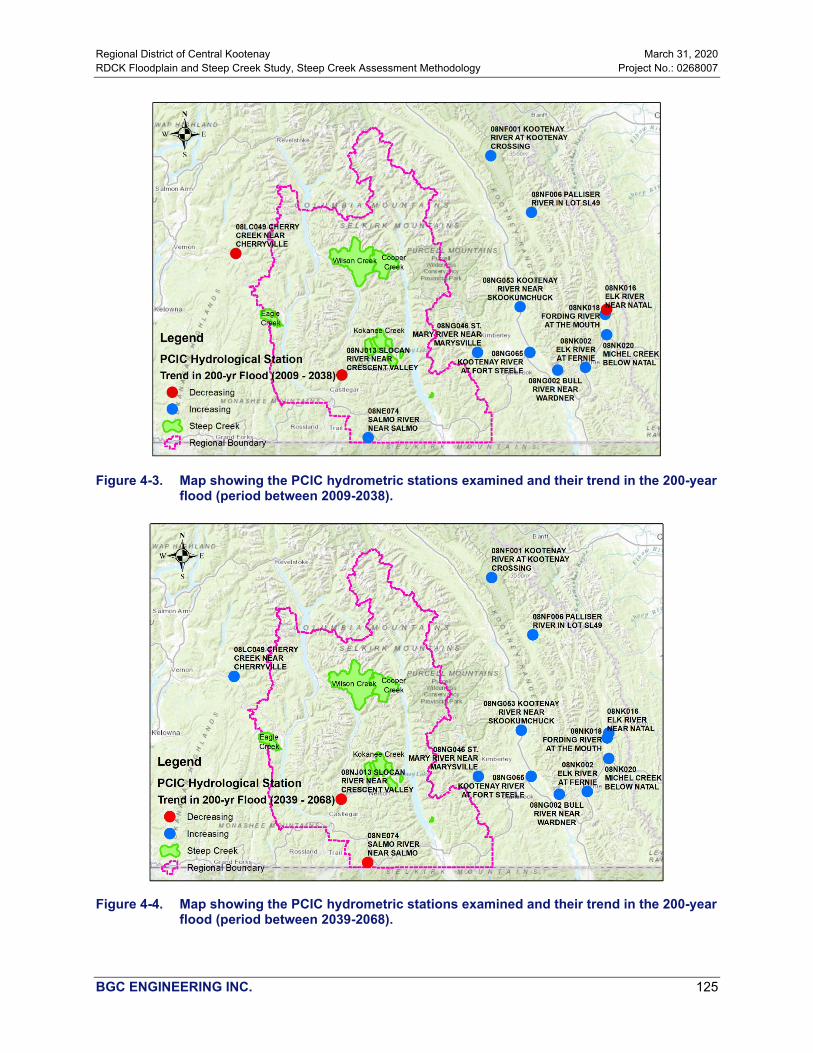
Regional District of Central Kootenay March 31, 2020 RDCK Floodplain and Steep Creek Study, Steep Creek Assessment Methodology Project No.: 0268007
BGC ENGINEERING INC. 125
Figure 4-3. Map showing the PCIC hydrometric stations examined and their trend in the 200-year
flood (period between 2009-2038).
Figure 4-4. Map showing the PCIC hydrometric stations examined and their trend in the 200-year
flood (period between 2039-2068).

Regional District of Central Kootenay March 31, 2020 RDCK Floodplain and Steep Creek Study, Steep Creek Assessment Methodology Project No.: 0268007
BGC ENGINEERING INC. 126
Figure 4-5. Map showing the PCIC hydrometric stations examined and their trend in the 200-year
flood (period between 2069-2098).
The maps show that, in general, most of the thirteen stations examined show an increase in the magnitude of the 200-year flood over time with some exceptions based on an assessment of the mean of the eight models. A bar chart of the results for the individual hydrometric stations is shown in Figure 4-6. The expected change in 200-year flood for the 2039-2068 period varies between -8.7% and +28.1% from the 1955-2009 period. For the 2069-2098 period, the range in the change of the 200-year flood magnitude increases from -6.7% and +59.7% from the 1955-2009 period. Boxplots of the results for the three periods for the eight model runs are provided in Figure 4-7 and Figure 4-8. The boxplots provide a sense of the uncertainty in the analysis by the considerable range in the estimated 200-year peak discharge. Of note, the PCIC Station Hydrologic Model Output was found to poorly predict historical peak discharges.

Regional District of Central Kootenay March 31, 2020 RDCK Floodplain and Steep Creek Study, Steep Creek Assessment Methodology Project No.: 0268007
BGC ENGINEERING INC. 127
Figure 4-6. Bar-graph of the PCIC hydrometric stations and their change in the magnitude of the
200-year flood for the three periods examined compared to the 1955-2009 historical period.
-20
-10
0
10
20
30
40
50
60
70Ch
ange
(%)
2009 - 2038 2039 - 2068 2069 - 2098

Regional District of Central Kootenay March 31, 2020 RDCK Floodplain and Steep Creek Study, Steep Creek Assessment Methodology Project No.: 0268007
BGC ENGINEERING INC. 128
Figure 4-7. Boxplots of the PCIC Hydrological Stations and their change in the magnitude of the 200-year flood for the three periods examined compared to the 1955-2009 historical period. Boxplots represent the interquartile range from the ensemble of 8 GCM models.

Regional District of Central Kootenay March 31, 2020 RDCK Floodplain and Steep Creek Study, Steep Creek Assessment Methodology Project No.: 0268007
BGC ENGINEERING INC. 129
Figure 4-8. Boxplots of the PCIC Hydrological Stations and their change in the magnitude of the 200-year flood (continued).

Regional District of Central Kootenay March 31, 2020 RDCK Floodplain and Steep Creek Study, Steep Creek Assessment Methodology Project No.: 0268007
BGC ENGINEERING INC. 130
4.4.3.2. Precipitation Assessment from Downscaled GCM Data
To investigate temporal trends in the intensity-duration-frequency (IDF) relationship under climate change, the simulated historical and projected daily precipitation data were retrieved for eight downscaled GCM models (1950 - 2100) provided by PCIC (2019)12 and summed for durations of 1, 2, 3, 5, and 7 days over each of the steep creek watersheds within the District. Annual maxima series were extracted considering the spring months of April, May and June only, in an attempt to represent rainfall events occurring on an isothermal snowpack, an expected flood-generating mechanism. Frequencies analyses were then performed over 30-year periods between 1961 to 2100 to support a qualitative (visual) assessment of temporal trends for the 2-, 20-, 50- and 100-year spring precipitation quantiles. Box-plots of the estimated change in the 1, 2, 3, 5 and 7 day cumulative precipitation for the eight ensemble models for RCP 8.5 as shown in Figure 4-9 to Figure 4-20.
The figures suggest that IDF quantiles saw an increase during the 1961-1990 and 1971-2000 historical period and then are projected to remain generally constant until 2050 followed by a marked increase in the intensity, itself followed by a decrease by 2080 for all five durations (no measurable difference in the intensity-frequency relation was observed between the different durations). It is suspected that this is change in the IDF relation between 2050 and 2080 is due to the Pacific Decadal Oscillation (PDO).
12 BGC was only able to successfully retrieve data from these eight models.

Regional District of Central Kootenay March 31, 2020 RDCK Floodplain and Steep Creek Study, Steep Creek Assessment Methodology Project No.: 0268007
BGC ENGINEERING INC. 131
Figure 4-9. Box-plots of the estimated change in the 1, 2, 3, 5 and 7 day cumulative precipitation between 1961 to 2100 for the eight ensemble models for RCP 8.5 for Redfish Creek. Box-plots represent the interquartile range from the ensemble of 8 GCM models.

Regional District of Central Kootenay March 31, 2020 RDCK Floodplain and Steep Creek Study, Steep Creek Assessment Methodology Project No.: 0268007
BGC ENGINEERING INC. 132
Figure 4-10. Box-plots of the estimated change in the 1, 2, 3, 5 and 7 day cumulative precipitation between 1961 to 2100 for the eight ensemble models for RCP 8.5 for Duhamel Creek. Box-plots represent the interquartile range from the ensemble of 8 GCM models.

Regional District of Central Kootenay March 31, 2020 RDCK Floodplain and Steep Creek Study, Steep Creek Assessment Methodology Project No.: 0268007
BGC ENGINEERING INC. 133
Figure 4-11. Box-plots of the estimated change in the 1, 2, 3, 5 and 7 day cumulative precipitation between 1961 to 2100 for the eight ensemble models for RCP 8.5 for Wilson Creek. Box-plots represent the interquartile range from the ensemble of 8 GCM models.

Regional District of Central Kootenay March 31, 2020 RDCK Floodplain and Steep Creek Study, Steep Creek Assessment Methodology Project No.: 0268007
BGC ENGINEERING INC. 134
Figure 4-12. Box-plots of the estimated change in the 1, 2, 3, 5 and 7 day cumulative precipitation between 1961 to 2100 for the eight ensemble models for RCP 8.5 for Sitkum Creek. Box-plots represent the interquartile range from the ensemble of 8 GCM models.
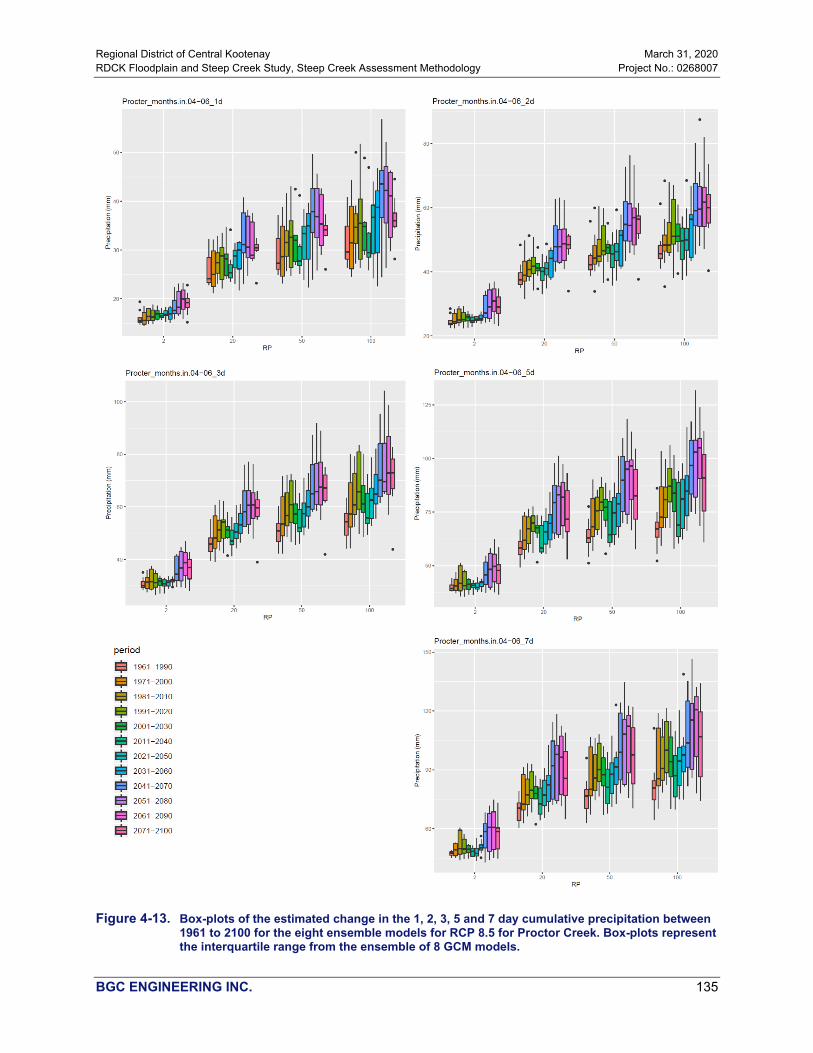
Regional District of Central Kootenay March 31, 2020 RDCK Floodplain and Steep Creek Study, Steep Creek Assessment Methodology Project No.: 0268007
BGC ENGINEERING INC. 135
Figure 4-13. Box-plots of the estimated change in the 1, 2, 3, 5 and 7 day cumulative precipitation between 1961 to 2100 for the eight ensemble models for RCP 8.5 for Proctor Creek. Box-plots represent the interquartile range from the ensemble of 8 GCM models.

Regional District of Central Kootenay March 31, 2020 RDCK Floodplain and Steep Creek Study, Steep Creek Assessment Methodology Project No.: 0268007
BGC ENGINEERING INC. 136
Figure 4-14. Box-plots of the estimated change in the 1, 2, 3, 5 and 7 day cumulative precipitation between 1961 to 2100 for the eight ensemble models for RCP 8.5 for Harrop Creek. Box-plots represent the interquartile range from the ensemble of 8 GCM models.

Regional District of Central Kootenay March 31, 2020 RDCK Floodplain and Steep Creek Study, Steep Creek Assessment Methodology Project No.: 0268007
BGC ENGINEERING INC. 137
Figure 4-15. Box-plots of the estimated change in the 1, 2, 3, 5 and 7 day cumulative precipitation between 1961 to 2100 for the eight ensemble models for RCP 8.5 for Cooper Creek. Box-plots represent the interquartile range from the ensemble of 8 GCM models.

Regional District of Central Kootenay March 31, 2020 RDCK Floodplain and Steep Creek Study, Steep Creek Assessment Methodology Project No.: 0268007
BGC ENGINEERING INC. 138
Figure 4-16. Box-plots of the estimated change in the 1, 2, 3, 5 and 7 day cumulative precipitation between 1961 to 2100 for the eight ensemble models for RCP 8.5 for Kuskonook Creek. Box-plots represent the interquartile range from the ensemble of 8 GCM models.
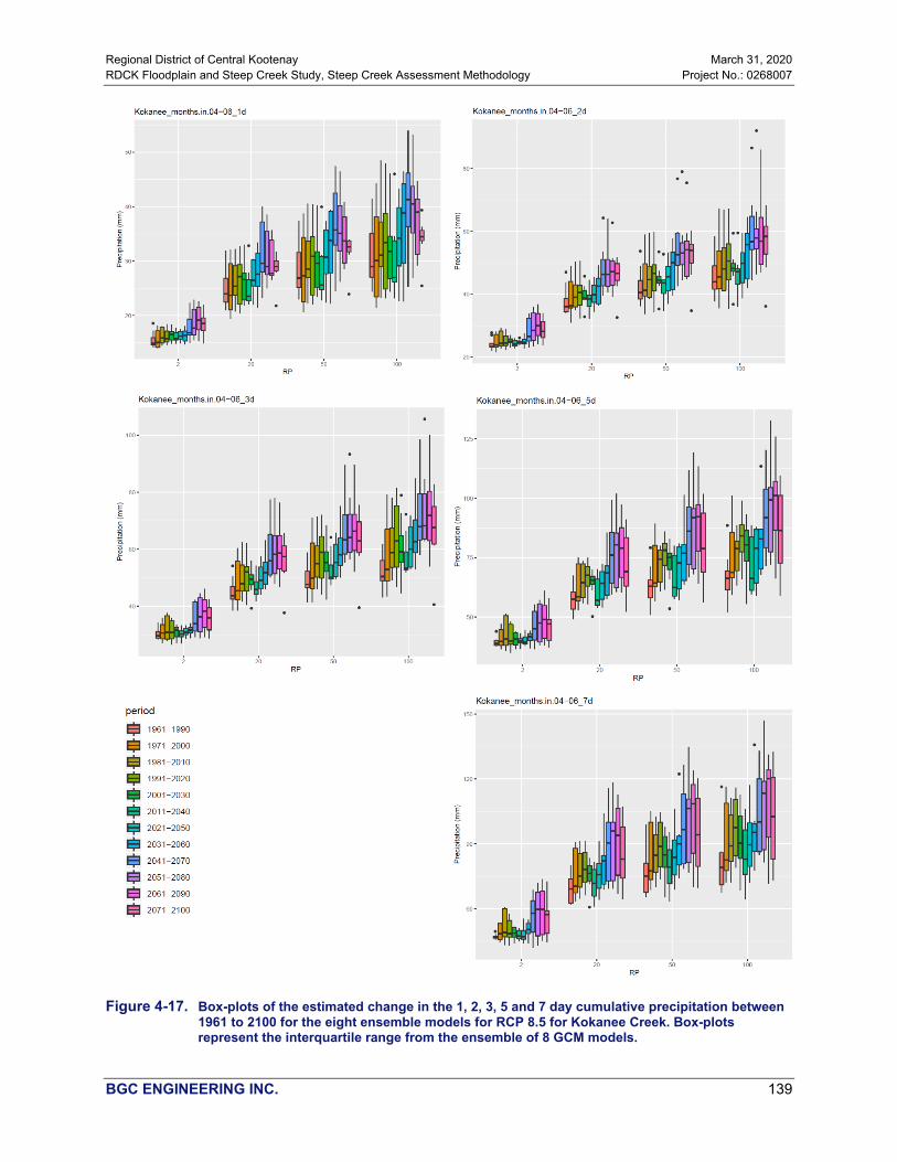
Regional District of Central Kootenay March 31, 2020 RDCK Floodplain and Steep Creek Study, Steep Creek Assessment Methodology Project No.: 0268007
BGC ENGINEERING INC. 139
Figure 4-17. Box-plots of the estimated change in the 1, 2, 3, 5 and 7 day cumulative precipitation between 1961 to 2100 for the eight ensemble models for RCP 8.5 for Kokanee Creek. Box-plots represent the interquartile range from the ensemble of 8 GCM models.

Regional District of Central Kootenay March 31, 2020 RDCK Floodplain and Steep Creek Study, Steep Creek Assessment Methodology Project No.: 0268007
BGC ENGINEERING INC. 140
Figure 4-18. Box-plots of the estimated change in the 1, 2, 3, 5 and 7 day cumulative precipitation between 1961 to 2100 for the eight ensemble models for RCP 8.5 for Eagle Creek. Box-plots represent the interquartile range from the ensemble of 8 GCM models.

Regional District of Central Kootenay March 31, 2020 RDCK Floodplain and Steep Creek Study, Steep Creek Assessment Methodology Project No.: 0268007
BGC ENGINEERING INC. 141
Figure 4-19. Box-plots of the estimated change in the 1, 2, 3, 5 and 7 day cumulative precipitation between 1961 to 2100 for the eight ensemble models for RCP 8.5 for Inonoaklin Creek. Box-plots represent the interquartile range from the ensemble of 8 GCM models.

Regional District of Central Kootenay March 31, 2020 RDCK Floodplain and Steep Creek Study, Steep Creek Assessment Methodology Project No.: 0268007
BGC ENGINEERING INC. 142
4.5. Summary
The EGBC guidelines, summarized in Section 4.4.1, offer procedures to account for climate change when flood magnitudes for protective works or mitigation procedures are required (EGBC, 2018). The guidelines recommend that at-site (or nearby) time-series data be analyzed for statistically significant trends. If a statistically significant trend is not detectable, the guidelines recommend that a 10% upward adjustment in design discharge is to be applied to account for likely future change in water input from precipitation. If a statistically significant trend is detectable the guidelines recommend three different procedures including consideration of 1) regionally downscaled projections of annual precipitation and snowpack magnitude, 2) adjustment of IDF curves for expected future precipitation, and or 3) adjustment of the expected flood magnitude and frequency according to the projected change in runoff during the life of the project, or by 20% in small drainage basins for which information of future local conditions is inadequate to provide reliable guidance.
For this study, the impacts of climate change on peak discharge estimates by 2050 (2041 to 2070) were assessed by BGC using statistical and processed-based methods. The statistical methods included a trend assessment on historical flood events using the Mann-Kendall test as well as the application of climate-adjusted variables (mean annual precipitation, mean annual temperature, and precipitation as snow) to the Regional FFA model. The process-based methods included a trend analysis for climate-adjusted flood and precipitation data offered by the PCIC.
The results of the statistical and process-based methods were found to be inconsistent across the RDCK by 2050 (2041 to 2070). Most of the discharge assessed from hydrological regions did not indicate statistically significant trends. The trends that were found were also not consistent with some showing an increasing trend while others a decreasing trend. The results of the statistical flood frequency modelling generally predict a small decrease in the flood magnitude, while the results of the process-based modelling of discharge generally show an increase with a wide range in magnitude. The results of the process-based assessment of the IDF quantiles show an increase during the 1961-1990 and 1971-2000 historical period and then are projected to remain generally constant until 2050. The wide range in magnitude can be a function of many variables including watershed characteristics (e.g., proportion of watershed elevation above a given threshold) which were not explicitly addressed in this assessment.
4.6. Conclusion
The climate change impact assessment results were difficult to synthesise in order to select climate-adjusted peak discharges on a site-specific basis. The assessment of the trends in the discharge records was inconclusive. The results of the statistical flood frequency modelling generally show a small decrease in the flood magnitude, while the results of the process-based discharge modelling generally show an increase with a wide range in magnitude. As a result, peak discharge estimates were adjusted upwards by 20% to account for the uncertainty in the impacts of climate change in the RDCK.

Regional District of Central Kootenay March 31, 2020 RDCK Floodplain and Steep Creek Study, Steep Creek Assessment Methodology Project No.: 0268007
BGC ENGINEERING INC. 143
5. CLOSURE We trust the above satisfies your requirements at this time. Should you have any questions or comments, please do not hesitate to contact us.
Yours sincerely,
BGC ENGINEERING INC. per:
Matthias Jakob, Ph.D., P.Geo. Matthias Busslinger, M.A.Sc., P.Eng. (BC) Principal Geoscientist Senior Geotechnical Engineer
Melissa Hairabedian, M.Sc., P.Geo. Senior Hydrologist
Reviewed by:
Hamish Weatherly, M.Sc., P.Geo. Principal Hydrologist
KH/HW/mp/sjk

Regional District of Central Kootenay March 31, 2020 RDCK Floodplain and Steep Creek Study, Steep Creek Assessment Methodology Project No.: 0268007
BGC ENGINEERING INC. 144
REFERENCES Ackers, P. & White, W.R. (1973). Sediment transport: New approach and analysis, Journal of
the Hydraulics Division, 99(hy11), 204-254. Ashworth, P.J. & Ferguson, R.I. (1989) Size-selective entrainment of bed load in gravel bed
streams. Water Resources Research, 25(4), 627-634. https://doi.org/10.1029/WR025i004p00627
Aulitzky, H. (1980) Vorläufige zweigeteilte Wildbachklassifikation (Preliminary two-fold classification of mountain torrents). Symposium Interpraevent 1980 (Vol. 4), 285-309.
Ballantyne, C.K. (2002). A general model of paraglacial landscape response. Quaternary Science Reviews, 21(8), 1935-2017. https://doi.org/10.1191/0959683602hl553fa
BGC Engineering Inc. (2014, March 7). Cougar Creek Debris Flood Hazard Assessment [Report]. Prepared for Town of Canmore.
BGC Engineering Inc. (2014, October 31). Three Sisters Creek Debris Flood Hazard Assessment [Report]. Prepared for Town of Canmore.
BGC Engineering Inc. (2015, March 1). Exshaw Creek and Jura Creek Debris Flood Risk Assessment [Report]. Prepared for Municipal District of Bighorn.
BGC Engineering Inc. (2015, May 22). Grotto Creek Debris-Flood Hazard Assessment [Report]. Prepared for Town of Canmore.
BGC Engineering Inc. (2019, November 15). NDMP Stream 2 Project Deliverables – Revised [Letter]. Prepared for Regional District of Central Kootenay.
Blair, T.C., & McPherson, J.G. (1994). Alluvial fans and their natural distinction from rivers based on morphology, hydraulic processes, sedimentary processes and facies assemblages. Journal of Sedimentary Research, A64, 450 – 489.
British Columbia Ministry of Environment. (2016). Indicators of climate change for British Columbia: 2016 update. Retrieved from https://www2.gov.bc.ca/assets/gov/environment/research-monitoring-and-reporting/reporting/envreportbc/archived-reports/climate-change/climatechangeindicators-13sept2016_final.pdf
Brunner, G. W., & CEIWR-HEC. (2016). HEC-RAS River Analysis System 2D Modeling User’s Manual. Retrieved from www.hec.usace.army.mil
Bufe, A., Turowski, J.M., Burbank, D., Paola, C., Tofelde, S. Wickert, A., & Hoffimann, J. (2019). Controls on the lateral channel-migration rate of braided channel systems in coarse non-cohesive sediment. Earth Surface Processes and Landforms, 44(14), 2823-2836
Bunte, K. Abt, S.R., Swingle, K.W., Cenderelli, D.A., & Schneider, M. (2013). Critical Shields values in coarse-bedded steep streams. Water Resources Research, 49(11), 7427-7447. https://doi.org/10.1002/2012WR012672
Burbank, D.W., & Anderson R.S. (2011). Tectonic Geomorphology (2nd ed.). https://onlinelibrary.wiley.com/doi/book/10.1002/9781444345063
Carling, P. (1988). The Concept of Dominant Discharge Applied to Two Gravel-Bed Streams in Relation to Channel Stability Thresholds. Earth Surface Processes and Landforms, 13(4), 355-367. https://doi.org/10.1002/esp.3290130407

Regional District of Central Kootenay March 31, 2020 RDCK Floodplain and Steep Creek Study, Steep Creek Assessment Methodology Project No.: 0268007
BGC ENGINEERING INC. 145
Cesca, M., & D’Agostino, V. (2008). Comparison between FLO-2D and RAMMS in debris-flow modelling: a case study in the Dolomites. Monitoring, Simulation, Prevention and Remediation of Dense Debris Flows II. doi: 10.2495/deb080201
Chow, V.T. (1959). Open Channel Hydraulics: New York: McGraw-Hill Church, M. & Jakob, M. (2020). What is a debris flood? Submitted to Water Resources
Research. Church, M. (2013). Steep headwater channels. In E. Wohl (Ed.), Shroder, J.F. (eds.) Treatise
on Geomorphology, (Vol. 9, pp. 528-549). San Diego: Academic Press. Church, M., & Ryder, J.M. (1972). Paraglacial sedimentation: a consideration of fluvial
processes conditioned by glaciation. Geological Society of America Bulletin, 83, 3059-3072. Coles, S. (2001). An introduction to statistical modeling of extreme values. London, UK:
Springer-Verlag Dalrymple, T. (1960). Flood frequency analysis (1543). Washington, DC.: U.S. G.P.O. Davidson, S.L. & Eaton, B.C. (2018). Beyond regime: A stochastic model of floods, bank
erosion, and channel migration. Water Resources Research, 54. https://doi.org/10.1029/2017WR022059
de Haas, T., Densmore, A.L., Stoffel, M., Suwa, H., Imaizumi, F., Ballesteros-Cánovas, J.A., & Wasklewicz, T. (2018). Avulsions and the spatio-temporal evolution of debris-flow fans. Earth-Science Reviews, 177, 53-75. https://doi.org/10.1016/j.earscirev.2017.11.007
Eaton, B., Mackenzie, L., Jakob, M., & Weatherly, H. (2017). Assessing erosion hazards due to floods on fans: Physical modeling and application to engineering challenges. Journal of Hydraulic Engineering, 143(8), https://ascelibrary.org/doi/10.1061/%28ASCE%29HY.1943-7900.0001318
Engineers and Geoscientists BC. (2017). Professional practice guidelines: Flood mapping in BC. Retrieved from https://www.egbc.ca/getmedia/8748e1cf-3a80-458d-8f73-94d6460f310f/APEGBC-Guidelines-for-Flood-Mapping-in-BC.pdf.aspx
Engineers and Geoscientists BC. (2018). Professional Practice Guidelines - Legislated Flood Assessments in a Changing Climate in BC. Version 2.1.
Farjad, B., Gupta, A., & Marceau, D.J. (2016). Annual and seasonal variations of hydrological processes under climate change scenarios in two sub-watersheds of a complex watershed. Water Resources Management, 30(8), 2851-2865. https://doi.org/10.1007/s11269-016-1329-3
Farr, T., Rosen, P., Caro, E. Crippen, R., Duren, R., Hensley, S.,…& Alsdorf, D. (2007). The shuttle radar topography mission. Reviews of Geophysics, 45(2). https://doi.org/10.1029/2005RG000183
FLO-2D Software, Inc. (2017). FLO-2D Reference Manual. Build No. 16 January 2017. Grant, G. (1997). Critical flow constrains flow hydraulics in mobile-bed streams: a new
hypothesis. Water Resources Research, 33(2), 349-358. 10.1029/96WR03134 Greenwood, J.A., Lanswehr, J.M., Matalas, N.C., & Wallis, J.R. (1979). Probability weighted
moments: Definition and relation to parameters of several distributions expressible in reserve form. Water Resources Research, 15, 1049-54.

Regional District of Central Kootenay March 31, 2020 RDCK Floodplain and Steep Creek Study, Steep Creek Assessment Methodology Project No.: 0268007
BGC ENGINEERING INC. 146
Griswold, J.P., & Iverson, R.M. (2008). Mobility Statistics and automated hazard mapping for debris flows and rock avalanches (version 1.1). Reston, Virginia: U.S. Geological Survey.
Guse, B., Thieken, A.H., Castellarin, A., & Merz, B. (2010). Deriving probabilistic regional envelope curves with two pooling methods. Journal of Hydrology, 380, 14-26. 10.1016/j.jhydrol.2009.10.010
Harder, P., Pomeroy, J.W., & Westbrook, C.J. (2015). Hydrological resilience of a Canadian Rockies headwaters basin subject to changing climate, extreme weather, and forest management. Hydrological Processes, 29, 3905-3924. https://doi.org/10.1002/hyp.10596
Holm, K., Jakob, M., Scordo, E., Strouth, A., Wang, R., & Adhikari, R. (2016). Identification, Prioritization, and Risk Reduction: Steep Creek Fans Crossed by Highways in Alberta. GeoVancouver 2016. Vancouver, Canada.
Hosking, J.R.M. (1990). L-Moments: Analysis and Estimation of Distributions Using Linear Combinations of Order Statistics. Journal of the Royal Statistical Society (Series B), 52, 105-124.
Hosking, J.R.M. & Wallis, J.R. (1997) Regional Frequency Analysis: An Approach Based on L-moments. Cambridge University Press, UK. http://dx.doi.org/10.1017/cbo9780511529443
Hosking, J.R.M., & Wallis, J.R. (1993). Some statistics useful in regional frequency analysis. Water Resources Research, 29(2), 271-281. https://doi.org/10.1029/92WR01980
Hungr, O., Evans, S.G., Bovis, M.J. Hutchinson, J.N. (2001). A review of the classification of the landslides of the flow type. Environmental and Engineering Geoscience, 7(3), 221-238.
Hungr, O., Leroueil, S., & Picarelli, L. (2014). The Varnes classification of landslide types, an update. Landslides, 11, 167-194. https://doi.org/10.1007/s10346-013-0436-y
Iverson, R.M. (1997). The physics of debris flows. Reviews of Geophysics, 35(3), 245-296. https://doi.org/10.1029/97RG00426
Iverson, R.M. (2014). Debris flows: behaviour and hazard assessment. Geology Today, 30(1), 15-20. https://doi.org/10.1111/gto.12037
Jakob, M. & Jordan, P. (2001). Design floods in mountain streams – the need for a geomorphic approach. Canadian Journal of Civil Engineering, 28(3), 425-439. https://doi.org/10.1139/l01-010
Jakob, M. (1996). Morphometric and geotechnical controls of debris flow frequency and magnitude in southwestern British Columbia (Ph.D. dissertation). Department of Geography, University of British Columbia, Vancouver, B.C.
Jakob, M., Bale, S., McDougall, S., & Friele, P. (2016). Regional debris-flow and debris-flood frequency magnitude curves. In GeoVancouver 2016, Proceedings of the 68th Canadian Geotechnical Conference. Richmond, BC: Canadian Geotechnical Society.
Jakob, M., Clague, J., & Church, M. (2016). Rare and dangerous: recognizing extra-ordinary events in stream channels. Canadian Water Resources Journal. 41, 161-173. https://doi.org/10.1080/07011784.2015.1028451
Jakob, M., Schnorbus, M., & Owen, T. (2018). Impacts of Climate Change on Debris-Flood Magnitude in the southern Rocky Mountains in Canada. Initial Findings. Geohazard7. Paper presented at meeting of the Canadian Geotechnical Society, Canmore, Alberta.
Jakob, M., Stein, D., & Ulmi, M. (2012). Vulnerability of buildings to debris flow impact. Natural Hazards, 60(2), 241-261. https://doi.org/10.1007/s11069-011-0007-2

Regional District of Central Kootenay March 31, 2020 RDCK Floodplain and Steep Creek Study, Steep Creek Assessment Methodology Project No.: 0268007
BGC ENGINEERING INC. 147
Jakob, M., Weatherly, H., Bale, S., Perkins, A., & MacDonald, B. (2017). Article A Multi-Faceted Debris-Flood Hazard Assessment for Cougar Creek, Alberta, Canada. Hydrology, 4(7). doi:10.3390/hydrology4010007
Jakob, M., Mark, E., McDougall, S., Friele, P., Lau, C.-A., & Bale, S. (in press). Regional debris-flow and debris-flood frequency-magnitude curves. Earth Surface Processes and Landforms.
Jarrett, R. (1984). Hydraulics of high-gradient streams. Journal of Hydraulic Engineering, 110(11). https://doi.org/10.1061/(ASCE)0733-9429(1984)110:11(1519)
Kellerhals, R. & Church, M. (1990). Hazard management on fans, with examples from British Columbia. In A.H. Rachocki & M. Church (Eds.), Alluvial fans: a field approach (pp. 335-354). Chichester, UK: John Wiley & Sons.
Klock, G.O. & Helvey, J.D. (1976) Debris flows following wildfire in North Central Washington. Proceedings of the 3rd Federal Inter-Agency Sedimentation Conference, March 22–25, Denver, Colorado (pp. 91–98). Water Resources Council, Denver, CO.
Knutti, R., Masson, D., & Gettelmen, A. (2013). Climate model genealogy: Generation CMIP5 and how we got there. Geophysical Research Letters, 40(6), 1194 -1199. https://doi.org/10.1002/grl.50256
Lane, E.W. (1955) Design of stable channels. American Society of Civil Engineers Transactions, 120, 1234-1279.
Latifovic, R., Homer, C., Ressl, R., Pouliot, D. Hossain, S.N., Colditz, R.R., Olthof, I., Giri, C., & Victoria, A. (2012). North American Land Change Monitoring System. In C. Giri (Ed) Remote Sensing of Land and Land Cover: Principles and Applications (p. 303-324). CRC Press.
Lau, C.A. (2017). Channel scour on temperate alluvial fans in British Columbia (Master’s thesis). Simon Fraser University, Burnaby, BC. Retrieved from http://summit.sfu.ca/system/files/iritems1/17564/etd10198_CLau.pdf
Loukas, A. & Quick, M.C. (1999). The effect of climate change on floods in British Columbia. Nordic Hydrology, 30(3), 231-256. https://doi.org/10.2166/nh.1999.0013
Mackenzie, L., Eaton, B., & Church, M. (2018). Breaking from the average: Why large grains matter in gravel-bed streams. Earth Surface Processes and Landforms, 43(15), 3190-3196.
Magirl, C., Hilldale, R., Curran, C., Duda, J., Straub, T., Domanski, M., & Foreman, J. (2015). Large-scale dam removal on the Elwha River, Washington, USA: Fluvial sediment load. Geomorphology, 246, 669-686.
Major, J., Pierson, T., & Scott, K. (2005). Debris flows at Mount St. Helens, Washington, USA. In M. Jakob & O. Hungr (Eds.), Debris-flow Hazards and Related Phenomena (pp. 685-731). Springer, Berlin Heidelberg.
Manville, V. & White, J.D.L. (2003). Incipient granular mass flows at the base of sediment-laden floods, and the roles of flow competence and flow capacity in the deposition of stratified bouldery sands. Sedimentary Geology, 155, 157-173.
Meyer, G.A. (2002) Fire in Western Conifer Forests: Geomorphic and Ecologic Processes and Climatic Drivers (Abstracts with Programs 34, p. 46). Geological Society of America, Boulder, CO.
Regional District of Central Kootenay March 31, 2020 RDCK Floodplain and Steep Creek Study, Steep Creek Assessment Methodology Project No.: 0268007
BGC ENGINEERING INC. 148
Ministry of Environment (MOE). (2016). Indicators of Climate Change for British Columbia. 2016 Update. June.
Moase, E., Strouth, A., & Mitchell, A. (2018). A comparison of different approaches for modeling a fine-grained debris flow. Paper presented at Second JTC1 Workshop on Triggering and Propagation of Rapid Flow-like Landslides, Hong Kong, Seton Portage, BC.
Montgomery, D.R. & Buffington, J.M. (1997). Channel-reach morphology in mountain drainage basins. Geological Society of America Bulletin, 109(5), 596-611. https://doi.org/10.1130/0016-7606(1997)109<0596:CRMIMD>2.3.CO;2
Mosbrucker, A.R. & Major, J.J. (2019) North Fork Toutle River debris flows initiated by atmospheric rivers. Paper presented at the joint Federal Interagency Sedimentation Conference and Federal Interagency Hydrologic Modeling Conference, Reno, NV. Retrieved from https://www.sedhyd.org/2019/openconf/modules/request.php?module=oc_program&action=view.php&id=202&file=1/202.pdf
North American Land Change Monitoring System (NALCMS), (2005). Interactive Pictorial Map of Land Cover Diversity in North America [Map]. From http://www.cec.org/tools-and-resources/north-american-environmental-atlas/north-american-land-change-monitoring-system
O’Brien, J.S. (1986). Physical process, rheology and modeling of mudflows (Ph.D. dissertation). Colorado State University, Fort Collins, CO.
Ouarda, T.B.M.J., St-Hilaire, A., & Bobée, B. (2008). Synthèse des développements récents en analyse régionale des extrêmes hydrologiques. Journal of Water Sciences, 21, 219–232. https://doi.org/10.7202/018467ar.
Pacific Climate Impacts Consortium (2014). Station Hydrologic Model Output. Downloaded from https://data.pacificclimate.org/portal/hydro_stn/map/ on November 2019.
Pacific Climate Impacts Consortium (PCIC) (2019). Statistically Downscaled Climate Scenarios. Downloaded from https://data.pacificclimate.org/portal/downscaled_gcms/map/ on November 2019. Method: BCCAQ v2.
Pacific Climate Impacts Consortium (PCIC). (2011). Hydrologic Impacts of Climate Change in the Peace, Campbell and Columbia Watersheds, British Columbia, Canada: Hydrologic Modeling Project Final Report (Part II).
Pacific Climate Impacts Consortium (PCIC). (2012). Plan2Adapt. Retrieved from https://www.pacificclimate.org/analysis-tools/plan2adapt.
Pacific Climate Impacts Consortium (PCIC). (2013). Climate Summary for: Kootenay / Boundary Region. Retrieved from https://www.pacificclimate.org/sites/default/files/publications/Climate_Summary-Kootenay-Boundary.pdf
Pacific Climate Impacts Consortium (PCIC). (2019). Plan2Adapt. Retrieved from https://www.pacificclimate.org/analysis-tools/plan2adapt.
Parker, G. (1978). Self-formed straight rivers with equilibrium banks and mobile bed. Part 2. The gravel river. Journal of Fluid Mechanics, 89, 127-146. https://doi.org/10.1017/S0022112078002505
Parker, G. (1979). Hydraulic geometry of active gravel rivers. ASCE Proceedings Journal of the Hydraulics Division, 105, 1185-1201.

Regional District of Central Kootenay March 31, 2020 RDCK Floodplain and Steep Creek Study, Steep Creek Assessment Methodology Project No.: 0268007
BGC ENGINEERING INC. 149
Pierson TC. (2005). Distinguishing between debris flows and floods from field evidence in small watersheds. Fact Sheet 2004-3142. U.S. Geological Survey.
Piton, G., & Recking, A. (2019). Steep bedload-laden flows: near critical?. Journal of Geophysical Research: Earth Surface, 124. 10.1029/2019JF005021
Prein, A.F., Rasmussen, R.M., Ikeda, K., Liu, C., Clark, M.P, & Holland, G.J. (2017). The future intensification of hourly precipitation extremes. Nature Climate Change, 7, 48-52. http://dx.doi.org/10.1038/nclimate3168
R Core Team. (2019). R: A language and environment for statistical computing. R Foundation for Statistical Computing, Vienna, Austria. https://www.R-project.org/.
Regent Instruments Inc. (2012). WinDENDRO [Computer software]. Canada. Rickenmann, D. (1990). Bedload transport capacity of slurry flows at steep slopes. PhD.
Thesis, ETH Zurich, https://doi.org/10.3929/ethz-a-000555802. Rickenmann, D. (2001). Comparison of bed load transport in torrents and gravel bed streams.
Water Resources Research, 37(12), 3295-3305. https://doi.org/10.1029/2001WR000319 Robson, A.J. & Reed, D.J. (1999). Statistical Procedures for Flood Frequency Estimation. Flood
Estimation Handbook, vol. 3. Institute of Hydrology, Wallingford, UK.
Ross, C.W., Prihodko, L., Anchang, J., Kumar, S., Ji, W., & Hanan, N.P. (2018). HYSOGs250m, global gridded hydrologic soil groups for curve-number-based runoff modeling. ORNL Distributed Active Archive Center. https://doi.org/10.3334/ORNLDAAC/1566.
Ryder, J.M. (1971a). Some aspects of the morphometry of paraglacial alluvial fans in south-central British Columbia. Canadian Journal of Earth Sciences, 8, 1252-1264. https://doi.org/10.1139/e71-114
Ryder, J.M. (1971b). The stratigraphy and morphology of paraglacial alluvial fans in south-central British Columbia. Canadian Journal of Earth Sciences, 8, 279-298. https://doi.org/10.1139/e71-027
Scheidl, C., & Rickenmann, D. (2010). Empirical prediction of debris-flow mobility and deposition on fans. Earth Surface Processes and Landforms, 35, 157-173.
Schnorbus, M. A., K. E. Bennett, A. T. Werner, & Berland, A. J. (2011). Hydrologic Impacts of Climate Change in the Peace, Campbell and Columbia Watersheds, British Columbia, Canada. Paper presented at the Pacific Climate Impacts Consortium, University of Victoria, Victoria, BC, 157 pp.
Schnorbus, M., Werner, A., & Bennett, K. (2014). Impacts of climate change in three hydrologic regimes in British Columbia, Canada. Hydrological Processes, 28, 1170-1189. https://doi.org/10.1002/hyp.9661
Schumm, S.A. (1977). The fluvial system. Wiley, New York. 338 pp. Shrestha, R. R., M. A. Schnorbus, A. T. Werner, & Berland, A. J. (2012): Modelling spatial and
temporal variability of hydrologic impacts of climate change in the Fraser River basin, British Columbia, Canada. Hydrol. Process., 26, 1840–1860, https://doi.org/10.1002/hyp.9283.
Sidle, R., & Onda, Y. (2004). Hydrogeomorphology: overview of an emerging science. Hydrological Processes, 18(4). 597-602.

Regional District of Central Kootenay March 31, 2020 RDCK Floodplain and Steep Creek Study, Steep Creek Assessment Methodology Project No.: 0268007
BGC ENGINEERING INC. 150
Smart, G.M. (1984). Sediment transport formula for steep channels. Journal of Hydraulic Engineering, 110, 267-276.
Stiny. (1931). Die geologischen Grundlagen der Verbauung der Geschiebeherde in Gewässern. Springer. Wien. Takahashi T. (1991). Debris Flows. Rotterdam, Balkema.
Tasker, G. (1980). Hydrologic regression with weighted least squares. Water Resources Research, 16(6), 1107-1113. https://doi.org/10.1029/WR016i006p01107
Tasker, G. (1982). Comparing methods of hydrologic regionalization. Water Resources Bulletin, 18(6), 965-970. https://doi.org/10.1111/j.1752-1688.1982.tb00102.x
Theule, J. I., Liébault, F., Laigle, D., Loye, A. and Jaboyedoff, M. (2015). Channel scour and fill by debris flows and bedload transport. Geomorphology, 243, 92-105. doi:10.1016/j.geomorph.2015.05.003.
United States Geological Survey (USGS). (1986). Urban hydrology for small watersheds. Technical report 55.
van Dijk, M., Kleinhans, M.G., Postma, G., & Kraal, E. (2012). Contrasting morphodynamics in alluvial fans and fan deltas: effects of the downstream boundary. Sedimentology, 59(7), 2125-2145. https://doi.org/10.1111/j.1365-3091.2012.01337.x
van Dijk, M., Postma, G., & Kleinhans, M.G. (2009). Autocyclic behaviour of fan deltas: an analogue experimental study. Sedimentology, 56(5), 1569-1589. https://doi.org/10.1111/j.1365-3091.2008.01047.x
Wang, T., Hamann, A. Spittlehouse, D.L., & Carroll, C. (2016). Locally downscaled and spatially customizable climate data for historical and future periods for North America. PLoS One 11, e0156720. https://doi.org/10.1371/journal.pone.0156720
Wang, Y. (2000). Development of methods for regional flood estimates in the province of British Columbia (Doctoral dissertation). Retrieved from University of British Columbia. 200 pp.
Ward, J.H. (1963). Hierarchical grouping to optimize an objective function. Journal of the American statistical association; 58(301), 236–244.
Werner, A. T., 2011: BCSD downscaled transient climate projections for eight select GCMs over British Columbia, Canada. Pacific Climate Impacts Consortium, University of Victoria, Victoria, BC, 63 pp.
Wilcock, P.R., & McArdell, B.W. (1993). Surface-based fractional transport rates: mobilization thresholds and partial transport of a sand-gravel sediment. Water Resources Research, 33(1). 10.1029/92WR02748
Wilcock, P.R., & McArdell, B.W. (1997). Partial transport of a sand/gravel sediment. Water Resources Research, 29(4). https://doi.org/10.1029/96WR02672
Wilford, D., Sakals, M., Innes, J., Sidle, R., & Bergerud, W. (2004). Recognition of debris flow, debris flood and flood hazard through watershed morphometrics. Landslides, 1. 61-66.
Wolman, G. (1954). A method of sampling coarse river-bed material. American Geophysical Union, 35(6), 951-956. https://doi.org/10.1029/TR035i006p00951
Wood, A. W., L. R. Leung, V. Sridhar, and Lettenmaier, D. P., (2004): Hydrologic implications of dynamical and statistical approaches to downscaling climate model outputs (link is external). Climate Change, 62, 189–216. https://doi.org/10.1023/B:CLIM.0000013685.99609.9e.

Regional District of Central Kootenay March 31, 2020 RDCK Floodplain and Steep Creek Study, Steep Creek Assessment Methodology Project No.: 0268007
BGC ENGINEERING INC. 151
Yue, S., Pilon, P., Phinney, B., & Cavadias, G. (2002). The influence of autocorrelation on the ability to detect trend in hydrological series. Hydrological Processes, 16, 1807-1829. 10.1002/hyp.1095
Zhang, Z., Stadnyk, T.A., & Burn, D.H. (2019). Identification of a preferred statistical distribution for at-site flood frequency analysis in Canada. Canadian Water Resources Journal. https://doi.org/10.1080/07011784.2019.1691942
Zeller, M.E. & Fullerton, W.T. (1983). A Theoretically Derived Sediment Transport Equation for Sand-Bed Channels in Arid Regions. In R. M. Li and P. F. Lagasse (Eds.), Proceedings of the D. B. Simons Symposium on Erosion and Sedimentation. Colorado State University and ASCE.
Zimmermann, A. (2010). Flow resistance in steep streams: An experimental study. Water Resources Research, 46. https://doi.org/10.1029/2009WR007913