steganography using stochastic di usion for the covert

Steganography using Stochastic Diffusion for theCovert Communication of Digital Images

Jonathan M Blackledge and AbdulRahman I Al-Rawi ∗

Abstract— This paper is devoted to the study of a

method called Stochastic Diffusion for encrypting dig-

ital images and embedding the information in another

host image or image set. We introduce the theoret-

ical background to the method and the mathemati-

cal models upon which it is based. This includes a

comprehensive study of the diffusion equation and its

properties leading to a convolution model for encrypt-

ing data with a stochastic field that is fundamental

to the approach considered. Two methods of imple-

menting the approach are then considered. The first

method introduces a lossy algorithm for hiding an im-

age in a single host image which is based on the bina-

rization of the encrypted data. The second method

considers a similar approach which uses three host

images to produce a near perfect reconstruction from

the decrypt. In both cases, details of the algorithms

developed are provide and examples given. The meth-

ods considered have applications for covert cryptog-

raphy and the authentication and self-authentication

of documents and full colour images.

Keywords: Image Encryption Information Hid-ing, Steganography, Stochastic Diffusion, Sym-metric Encryption

1 Introduction

The relatively large amount of data contained in digi-tal images makes them a good medium for undertakinginformation hiding. Consequently digital images can beused to hide messages in other images. A colour imagetypically has 8-bits to represent the red, green and bluecomponents for 24-bit colour images. Each colour com-ponent is composed of 256 colour values and the modifi-cation of some of these values in order to hide other datais undetectable by the human eye. This modification isoften undertaken by changing the least significant bit inthe binary representation of a colour or grey level value(for grey level digital images). For example, the grey levelvalue 128 has the binary representation 10000000. If we

∗Information and Communications Security Research Group,Dublin Institute of Technology, Kevin Street, Dublin 8, Ireland.

change the least significant bit to give 10000001 (whichcorresponds to a grey level value of 129) then the differ-ence in the output image will not be discernable. Hence,the least significant bit can be used to encode informationother than pixel intensity. If this is done for each colourcomponent then a single letter can be represented usingjust three pixels. The larger the host image comparedwith the hidden message, the more difficult it is to detectthe message. The host image represents the key to recov-ering the hidden image. Rather than the key being usedto generate a random number stream using a pre-definedalgorithm from which the stream can be re-generated (forthe same key), the digital image is, in effect, being usedas the cipher.

The large majority of methods developed for image in-formation hiding do not include encryption of the hiddenimage. In this paper we consider an approach in which ahidden image is encrypted by diffusion with a noise fieldbefore being embedded in the host image. The paperprovides a short survey on encrypted information hidingand then presents a detailed account of the mathematicalfoundations upon which the method, known as StochasticDiffusion, is based. Two applications are then consider:(i) Lossy information hiding which is based on the bina-risation of the encrypted field; (ii) Lossless informationhiding which is based on using three separate host im-ages in which the encrypted information is embedded.The methods considered have a range of applications indocument and full colour image authentication.

2 Survey on Encrypted Information Hid-ing

Compared with information hiding in general, there arerelatively few publications that have addressed the is-sue of hiding encrypted information. We now provide anoverview of some recent publications in this area.

In [1], a novel method is proposed for hiding the transmis-sion of biometric images based on chaos and image con-tent. To increase the security of the watermark, it is firstencrypted using a chaotic map where the keys used forencryption are generated from a palm print image. The

IAENG International Journal of Applied Mathematics, 41:4, IJAM_41_4_02

(Advance online publication: 9 November 2011)

______________________________________________________________________________________

pixel value distribution, illumination and various imagedistortions are different for each palm print image (even ifthey are for the same person) because the palm print im-age is different each time the image is captured. In [1], thenormalized mean value of three randomly selected pixelsfrom the palm print image is used as an initial conditionfor the chaotic map. The logistic map is used to gener-ate a one-dimensional sequence of real numbers which arethen mapped into a binary stream to encrypt the water-mark using an XOR operation. The encrypted watermarkis then embedded into the same palm print image usedto derive the secret keys. The stego-palm print image ishidden into the cover image using a novel content-basedhidden transmission scheme. First the cover image is seg-mented into different regions using a classical watershedalgorithm. Due to the over-segmentation resulting fromthis algorithm, a Region-based Fuzzy C-means Clusteringalgorithm is used to merge similar regions. The entropy ofeach region is then calculated and the stego-palm printimage embedded into the cover image according to theentropy value with more information being embedded inhighly textured regions compared to uniform regions. Athreshold value T is used to partition the two regions. Ifthe entropy is greater than T , the binary streams of thesecret data are inserted into the 4 least significant bitsof the region, and if the entropy is smaller than T , thebinary streams of the secret data are inserted into the 2least significant bits of the region. Colour host imagesare decomposed into RGB channels before embedding.

In [2] a method of hiding the transmission of biometricimages based on chaos and image content is proposed thatis similar to [1]. The secret data is a grayscale image ofsize 128 × 128 and before encrypting it, it is convertedinto a binary stream with the logistic map being used forencryption. The encryption keys used to produce the lo-gistic chaotic map sequence are generated randomly usingany pseudo random number generating algorithm. Theauthors use 256×256 color images as hosts which are con-verted into grayscale images and segmented into differentregions using the watershed algorithm to eliminate over-segmentation. A Fuzzy C-means Clustering algorithm isused to implement similar region merging. Each regionis classified into a certain cluster based on the regionsof the watershed lines. A k-nearest neighbour methodis used to partition the regions needing re-segmentation.For the resultant image without watershed lines, the en-tropy is calculated and the secret image is embedded ac-cording to the entropy values. The colour host image isdecomposed into RGB channels for embedding. Highlytextured regions are used to embed more information anda threshold value T is used to separate the two regions.If the entropy is smaller than T the binary streams of thesecret data are inserted into the 2 Least Significant Bits

(LSB) of the three channels of the region. If the entropyis greater than T , the binary streams of the secret dataare inserted into the 4 LSB of the three channels of theregion.

Another steganographic method is proposed in [3] forPNG images based on the information sharing tech-nique. The secret image M is divided into shares us-ing a (k, n)-threshold secret sharing algorithm. Secretshares are then embedded into the alpha-channel of thePNG cover image. The image M is first divided intot-bit segments which transforms each segment into a dec-imal number resulting in a decimal number sequence. A(4, 4)-threshold secret sharing algorithm is used to gen-erate ‘partial shares’ which are then embedded into thehost image by replacing the alpha-channel values of thehost image with the values of the shares. The process isrepeated for all decimal values of the secret data resultingin a stego-image. In general, if every four t-bit segmentsare transformed and embedded similarly, then the datahiding capacity is proportional to the chosen value of t inproportion to the dimension of the cover image. However,the larger the value of t the lower the visual quality ofthe stego-image which causes a wider range of the alpha-channel values to be altered leading to a more obviousnon-uniform transparency effect appearing on the stego-image. The value of t is therefore selected to ensure auniform distribution of the stego-image alpha-channel.

The principle of image scrambling and information hidingis introduced in [4] in which a double random scramblingscheme based on image blocks is proposed. A secret im-age of size M × N is divided into small sub-blocks ofsize 4 × 4 or 8 × 8, for example, and a scrambling algo-rithm used to randomize the sub-blocks using a given key.However, because the information in each inner sub-blockremains the same, another scrambling algorithm is usedwith a second key to destroy the autocorrelation in eachinner sub-block thereby increasing the difficulty of decod-ing the secret image. To make the hidden secret imagemore invisible, its histogram is compressed into a smallrange. Image hiding is then performed by simply addingthe secret image to the cover image. The hidden imageis recovered by expanding the histogram after extractionand decryption carried out for both the sub-blocks andinner sub-blocks to obtain a final reconstruction.

3 Diffusion and Confusion

The purpose of this section is to introduce the reader tosome of the basic mathematical models associated withthe processes of diffusion and confusion as based on thephysical origins of these processes. This provides a the-oretical framework for two of the principal underlying



______________________________________________________________________________________

concepts of cryptology in general as used in a variety ofcontexts.

In terms of plaintexts, diffusion is concerned with theissue that, at least on a statistical basis, similar plain-texts should result in completely different ciphertextseven when encrypted with the same key [5], [6]. Thisrequires that any element of the input block influencesevery element of the output block in an irregular fashion.

In terms of a key, diffusion ensures that similar keys resultin completely different ciphertexts even when used for en-crypting the same block of plaintext. This requires thatany element of the input should influence every elementof the output in an irregular way. This property must alsobe valid for the decryption process because otherwise anattacker may be able to recover parts of the input froman observed output by a partially correct guess of the keyused for encryption. The diffusion process is a functionof sensitivity to initial conditions that a cryptographicsystem should have and further, the inherent topologicaltransitivity that the system should also exhibit causingthe plaintext to be mixed through the action of the en-cryption process.

Confusion ensures that the (statistical) properties ofplaintext blocks are not reflected in the correspondingciphertext blocks. Instead every ciphertext must have arandom appearance to any observer and be quantifiablethrough appropriate statistical tests. Diffusion and con-fusion are processes that are of fundamental importancein the design and analysis of cryptological systems, notonly for the encryption of plaintexts but for data trans-formation in general.

3.1 The Diffusion Equation

In a variety of physical problem, the process of diffusioncan be modelled in terms of certain solutions to the dif-fusion equation whose basic homogeneous form is givenby [7] - [10]

∇2u(r, t) = σ∂

∂tu(r, t), σ =

1D

where D is the ‘Diffusivity’ and u is the diffused fieldwhich describes physical properties such as temperature,light, particle concentration and so on; r denotes the spa-tial vector and t denotes time.

The diffusion equation describes fields u that are the re-sult of an ensemble of incoherent random walk processes,i.e. walks whose direction changes arbitrarily from onestep to the next and where the most likely position aftera time t is proportional to

√t. Note that if u(r, t) is a

solution to the diffusion equation the function u(r,−t) isnot, i.e. it is a solution of the quite different equation,

∇2u(r,−t) = −σ ∂∂tu(r,−t).

Thus, the diffusion equation differentiates between pastand future. This is because the diffusing field u repre-sents the behaviour of some average property of an en-semble of many elements which cannot in general go backto their original state. This fundamental property of dif-fusive processes has a synergy with the use of one-wayfunctions in cryptology, i.e. functions that, given an in-put, produce an output that is not reversible - an outputfrom which it is not possible to compute the input.

Consider the process of diffusion in which a source of ma-terial diffuses into a surrounding homogeneous medium,the material being described by some initial conditionu(r, 0) say. Physically, it is to be expected that the mate-rial will increasingly ‘spread out’ as time evolves and thatthe concentration of the material decreases further awayfrom the source. The general solution to the diffusionequation yields a result in which the spatial concentra-tion of material is given by the convolution of the initialcondition with a Gaussian function, the time evolutionof this process being governed by the same process. Thissolution is determined by considering how the process ofdiffusion responds to a single point source which yieldsthe Green’s function (in this case, a Gaussian function).

3.2 Green’s Function for the DiffusionEquation

We evaluate the Green’s function [10]-[12] for for the dif-fusion equation satisfying the causality condition

G(r | r0, t | t0) = 0 if t < t0

where r | r0 ≡| r − r0 | and t | t0 ≡ t − t0. This can beaccomplished for one-, two- and three-dimensions simul-taneously [8]. Thus with R =| r− r0 | and τ = t− t0 werequire the solution of the equation(

∇2 − σ ∂

∂τ

)G(R, τ) = −δn(R)δ(τ), τ > 0

where n is 1, 2 or 3 depending on the number of dimen-sions and δ is the corresponding Dirac delta function [13]- [15]. One way of solving this equation is first to take theLaplace transform with respect to τ , then solve for G (inLaplace space) and then inverse Laplace transform theresult [16]. This requires an initial condition to be speci-fied (the value of G at τ = 0). Another way to solve thisequation is to take its Fourier transform with respect to



______________________________________________________________________________________

R, solve for G (in Fourier space) and then inverse Fouriertransform the result [17], [18]. Here, we adopt the latterapproach. Let

G(R, τ) =1

(2π)n

∞∫−∞

G(k, τ) exp(ik ·R)dnk

and

δn(R) =1

(2π)n

∞∫−∞

exp(ik ·R)dnk.

Then the equation for G reduces to

σ∂G

∂τ+ k2G = δ(τ)

where k =| k | which has the solution

G =1σ

exp(−k2τ/σ)H(τ)

where H(τ) is the step function

H(τ) =

{1, τ > 0;0, τ < 0.

Hence, the Green’s functions are given by

G(R, τ) =1

σ(2π)nH(τ)

∞∫−∞

exp(ik ·R) exp(−k2τ/σ)dnk

=1

σ(2π)nH(τ)

∞∫−∞

exp(ikxRx) exp(−k2xτ/σ)dkx

...

By rearranging the exponent in the integral, it becomespossible to evaluate each integral exactly. Thus, with

ikxRx − k2x

τ

σ= −

(kx

√τ

σ− iRx

2

√σ

τ

)2

−(σR2

x

4τ

)

= − τσξ2 −

(σR2

x

4τ

)where

ξ = kx − iσRx2τ

.

The integral over kx becomes

∞∫−∞

exp[−( τσξ2)−(σRx4τ

)]dξ

= e−(σR2x/4τ)

∞∫−∞

e−(τξ2/σ)dξ

=√πσ

τexp

[−(σR2

x

4τ

)]with similar results for the integrals over ky and kz givingthe result

G(R, τ) =1σ

( σ

4πτ

)n2

exp[−(σR2

4τ

)]H(τ).

The function G satisfies an important property which isvalid for all n:∫ ∞

−∞g(R, τ)dnr =

1σ

; τ > 0.

This is the expression for the conservation of the Green’sfunction associated with the diffusion equation. For ex-ample, if we consider the diffusion of heat, then if at atime t0 and at a point in space r0 a source of heat is in-troduced, then the heat diffuses out through the mediumcharacterized by σ in such a way that the total flux ofheat energy is unchanged.

3.3 Green’s Function Solution

Working in three dimensions, we consider the Green’ssolution to the inhomogeneous diffusion equation [8], [9](

∇2 − σ ∂∂t

)u(r, t) = −S(r, t)

where S is a source of compact support (r ∈ V ) and definethe Green’s function as the solution to the equation(∇2 − σ ∂

∂t

)G(r | r0, t | t0) = −δ3(r− r0)δ(t− t0).

The function S describes a source that is being diffused -a source of heat, for example - and is taken to be localisedin space.

It is convenient to first take the Laplace transform ofthese equations with respect to τ = t− t0 to obtain

∇2u− σ[−u0 + pu] = −S

and∇2G+ σ[−G0 + pG] = −δ3

where

u(r, p) =

∞∫0

u(r | r0, τ) exp(−pτ)dτ,

G(r, p) =

∞∫0

G(r | r0, τ) exp(−pτ)dτ,



______________________________________________________________________________________

S(r, p) =

∞∫0

S(r, τ) exp(−pτ)dτ,

u0 ≡ u(r, τ = 0) and G0 ≡ G(r | r0, τ = 0) = 0.

Pre-multiplying the equation for u by G and the equationfor G by u, subtracting the two results and integratingover V we obtain∫

V

(G∇2u− u∇2G)d3r + σ

∫V

u0Gd3r

= −∫V

SGd3r + u(r0, τ).

Using Green’s theorem [19], i.e. given that (Gauss’ theo-rem for any vector F)∫

V

∇ · Fd3r =∮S

F · nd2r

where S is the surface that encloses a volume V and nis a unit vector perpendicular to the surface element d2r,then, for two scalars f and g∫

V

(f∇2g − g∇2f)d3r =∫V

∇ · (f∇g − g∇f)d3r

=∮S

(f∇g − g∇f) · nd2r

and rearranging the result gives

u(r0, p) =∫V

S(r, p)G(r | r0, p)d3r

+σ∫V

u0(r)G(r | r, p)d3r +∮S

(g∇u− u∇g) · nd2r

Finally, taking the inverse Laplace transform and usingthe convolution theorem for Laplace transforms, we canwrite

u(r0, τ) =

τ∫0

∫V

S(r, τ ′)G(r | r0, τ − τ ′)d3rdτ ′

+σ∫V

u0(r)G(r | r0, τ)d3r

+

τ∫0

∮S

G(r | r0, τ′)∇u(r, τ − τ ′) · nd2rdτ ′

−τ∫

0

∮S

u(r, τ ′)∇G(r | r0, τ − τ ′) · nd2rdτ ′.

The first two terms are convolutions of the Green’s func-tion with the source function S and the initial conditionu(r, τ = 0), respectively.

If we consider the equation for the Green’s function(∇2 − σ ∂

∂t

)G(r | r0, t | t0) = −δ3(r− r0)δ(t− t0)

together with the equivalent time reversed equation(∇2 + σ

∂

∂t

)G(r | r1,−t | −t1) = −δ3(r− r1)δ(t− t1),

then pre-multiplying the first equation by G(r | r1,−t |−t1) and the second equation by G(r | r0, t | t0), sub-tracting the results and integrate over the volume of in-terest and over time t from −∞ to t0 then, using Green’stheorem, we obtain

t0∫−∞

dt

∮S

G(r | r1,−t | t1)∇G(r | r0, t | t0) · nd2r

−t0∫

−∞

dt

∮S

G(r | r0, t | t0)∇G(r | r1,−t | −t1) · nd2r

−σ∫V

d3r

t0∫−∞

dtG(r | r1,−t | −t1)∂

∂tG(r | r0, t | t0)

−σ∫V

d3r

t0∫−∞

dtG(r | r0, t | t0)∂

∂tG(r | r1,−t | −t1)

= G(r1 | r0, t1 | t0)−G(r0 | r1,−t0 | −t1).

If we then consider the Green’s functions and their gradi-ents to vanish at the surface S (homogeneous boundaryconditions) then the surface integral vanishes1. The sec-ond integral is∫

V

d3r [G(r | r1,−t | −t1)G(r | r0, t | t0)]t0t=−∞

and sinceG(r | r0, t | t0) = 0, t < t0

thenG(r | r0, t | t0 |t=−∞= 0.

AlsoG(r | r1,−t | −t1) |t=t0= 0

for t in the range of integration given. Hence,

G(r1 | r0, t1 | t0) = G(r | r1,−t0 | −t1).

This is the reciprocity theorem of the Green’s functionfor the diffusion equation.

1This is also the case if we consider an infinite domain



______________________________________________________________________________________

3.4 Infinite Domain Solution

In the infinite domain, the surface integral is zero and wecan work with the solution

u(r0, τ) =

τ∫0

∫V

S(r, τ ′)G(r | r0, τ − τ ′)d3rdτ ′

+σ∫V

u0(r)G(r | r0, τ)d3r

which requires that the spatial extent of the source func-tion is infinite but can include functions that are localisedprovided that S → 0 as | r |→ ∞ - a Gaussian functionfor example. The solution is composed of two terms. Thefirst term is the convolution (in space and time) of thesource function with the Green’s function and the secondterm is the convolution (in space only) of the initial con-dition u(r, 0) with the same Green’s function. We canwrite this result in the form

u(r, t) = G(| r |, t)⊗r ⊗tS(r, t) + σG(| r |, t)⊗r u(r, 0)

where ⊗r denotes the convolution over r and ⊗t denotesthe convolution over t.

In the case where we consider the domain of interest overwhich the process of diffusion occurs to be infinite in ex-tent, the solution to the homogeneous diffusion equation(when the source function is zero) specified as

∇2u(r, t)− σ ∂∂tu(r, t) = 0, u(r, 0) = u0(r)

is given by the convolution of the Green’s function withu0, i.e.

u(r0, t) = σG(| r |, t)⊗r u0(r), t > 0

Thus, in one-dimension, the solution reduces to

u(x, t) =√

σ

4πσtexp

[−σx

2

4t

]⊗x u0(x), t > 0

where ⊗x denotes the convolution integral over indepen-dent variable x and we see that the field u at a time t > 0is given by the convolution of the field at time t = 0 withthe one-dimensional Gaussian function√

σ

4πtexp

(−σx

2

4t

).

In two-dimensions, the result is

u(x, y, t) =σ

4πtexp

(− σ

4t[x2 + y2]

)⊗x⊗yu0(x, y), t > 0.

Ignoring scaling by the function σ/(4πt), we can writethis result in the form

u(x0, y0) = exp[− σ

4t(x2 + y2)

]⊗x ⊗yu0(x, y)

Thus, the field at time t > 0 is given by the field attime t = 0 convolved with the two-dimensional Gaussianfunction

exp[− σ

4t(x2 + y2)

].

This result can, for example, be used to model the dif-fusion of light through a diffuser that generates multiplelight scattering processes.

4 Diffusion from a Stochastic Source

For the case when(∇2 − σ ∂

∂t

)u(r, t) = −S(r, t), u(r, 0) = 0

the solution is

u(r, t) = G(| r |, t)⊗r ⊗tS(r, t), t > 0

If a source is introduced in terms of an impulse in time,then the ‘system’ will react accordingly and the diffuse fort > 0. This is equivalent to introducing a source functionof the form

S(r, t) = s(r)δ(t).

The solution is then given by

u(r, t) = G(| r |, t)⊗r s(r), t > 0.

Observe that this solution is of the same form as thehomogeneous case with initial condition u(r, 0) = u0(r)and the solution for initial condition u(r, 0) = u0(r) isgiven by

u(r, t) = G(| r |, t)⊗r [s(r) + u0(r)]

= G(| r |, t)⊗r u0(r) + n(r, t), t > 0

wheren(r, t) = G(| r |, t)⊗r s(r)

If s is a stochastic function (i.e. a random dependentvariable characterised, at least, by a Probability Den-sity Function (PDF) denoted by Pr[s(r)]), then n willalso be a stochastic function. Note, that for the time-independent source function S(r), we can construct aninverse solution (see Appendix A) given by

u0(r) = u(r, T )

+∞∑n=1

(−1)n

n![(DT )n∇2nu(r, T ) +D−1∇2n−2S(r)]



______________________________________________________________________________________

and that if S is a stochastic function, then the field u0

can not be recovered because the functional form of Sis not known. Thus, any error or noise associated withdiffusion leads to the process being irreversible - a ‘one-way’ process. This, however, depends on the magnitudeof the diffusivity D which for large values cancels out theeffect of any noise, thus making the process reversible, aneffect that is observable experimentally in the mixing oftwo highly viscous fluids, for example.

The inclusion of a stochastic source function provides uswith a self-consistent introduction to another importantconcept in cryptology, namely ‘confusion’. Taking, forexample, the two-dimensional case, the field u is given by(with scaling)

u(x, y) =1

4πtexp

[− σ

4t(x2 + y2)

]⊗x⊗yu0(x, y)+n(x, y).

We thus arrive at a basic model for the process of diffusionand confusion, namely

Output=Diffusion+Confusion.

Here, diffusion involves the ‘mixing’ of the initial con-dition with a Gaussian function and confusion is com-pounded in the addition of a stochastic or noise functionto the diffused output. The relative magnitudes of thetwo terms determines the dominating effect. As the noisefunction n increases in amplitude relative to the diffusionterm, the output will become increasingly determined bythe effect of confusion alone. In the equation above, thiswill occur as t increases since the magnitude of the dif-fusion term depends of the scaling factor 1/t. This isillustrated in Figure 1 which shows the combined effectof diffusion and confusion for an image of the phrase

Confusion+

Diffusion

as it is (from left to right and from top to bottom) pro-gressively diffused (increasing values of t) and increas-ingly confused for a stochastic function n that is uni-formly distributed.

The specific characteristics of the diffusion process con-sidered here is determined by an approach that is basedon modelling the system in terms of the diffusion equa-tion; the result being determined by the convolution ofthe initial condition with a Gaussian function. The pro-cess of confusion is determined by the statistical char-acteristics of the stochastic function n, i.e. its PDF.Stochastic functions with different PDFs will exhibit dif-ferent characteristics with regard to the level of confusion

inherent in the process as applied. In the example givenin Figure 1, uniformly distributed noise has been used.Gaussian or ‘normal’ distributed noise is more commonby virtue of fact that noise in general is the result ofan additive accumulation of many statistically indepen-dent random processes combining to form a normal orGaussian distributed field. Knowledge of the noise field,

Figure 1: Progressive diffusion and confusion of an image(top-left) - from left to right and from top to bottom -for uniform distributed noise. The convolution is under-taken using the convolution theorem and a Fast FourierTransform (FFT)

in particular, its PDF, provides a statistical approachto reconstructing the data based on the application ofBayesian estimation. For a Gaussian distributed noisefield with a standard deviation of σn and a data field u0

modelled in terms of Gaussian deviates with a standarddeviation of σu, the estimate u0(x, y) of u0(x, y) is givenby [20], [21]

u0(x, y) = q(x, y)⊗x ⊗yu(x, y)

where

q(x, y) =1

(2π)2

∫ ∫dkxdky exp(ikxx) exp(ikyy)

× G∗(kx, ky)| G(kx, ky) |2 +σ2

n/σ2u

and

G(kx, ky) =1

4πt

∫ ∫dxdy exp(ikxx) exp(ikyy)

× exp[− σ

4t(x2 + y2)

]Figure 2 illustrates the effect of applying this result to twodigital outputs (using a Fast Fourier Transform) with lowand high levels of noise, i.e. two cases for times t1 (low)and t2 > t1 (high). This example shows the effect of



______________________________________________________________________________________

increasing the level of confusion that occurs with increas-ing time t on the output of the reconstruction clearlyillustrating that it is not possible to recover u0 to anydegree of information assurance. This example demon-strates that the addition of a stochastic source functionto an otherwise homogeneous diffusive process introducesa level of error (as time increases) from which is it not pos-sible to recover the initial condition u0. From a physicalpoint of view, this is indicative of the fact that diffusiveprocess are irreversible. From an information theoreticview point, Figure 2 illustrated that knowledge of thestatistics of the stochastic field is not generally sufficientto recover the information we require. This is consistentwith the basic principle of data processes - Rubbish inGives Rubbish Out, i.e. given that

p(x, y) =1

4πtexp

[− σ

4t(x2 + y2)

],

the (Signal-to-Noise) ratio

‖p(x, y)⊗x ⊗yu0(x, y)‖‖n(x, y)‖

tends to zero as t increases. In other words, the longer thetime taken for the process of diffusion to occur, the morethe output is dominated by confusion. This is consistentwith all cases when the level of confusion is high and whenthe stochastic field used to generate this level of confusionis unknown (other than knowledge of its PDF). However,if the stochastic function has been synthesized2 and isthus known a priori, then we can compute

u(x, y)−n(x, y) =1

4πtexp

[− σ

4t(x2 + y2)

]⊗x⊗yu0(x, y)

from which u0 can be computed via application of theconvolution theorem to design an appropriate inverse fil-ter.

5 Stochastic Fields

By considering the diffusion equation for a stochasticsource, we have derived a basic model for the ‘solutionfield’ or ‘output’ u(r, t) in terms of the initial conditionor input u0(r) given by

u(r) = p(r)⊗r u0(r) + n(r)

where p is the PSF given by (with a = σ/4t)

exp(−a | r |2

)and n - which is taken to denote noise - is a stochasticfield, i.e. a random variable [22]. We shall now considerthe principal properties of stochastic fields, consideringthe case where the fields are random variables that arefunctions of time t.

2The synthesis of stochastic functions is a principal issue in cryp-tology.

Figure 2: Bayesian reconstructions (right) for data (left)with low (above) and high (below) levels of confusion.

5.1 Independent Random Variables

Two random variables f1(t) and f2(t) are independent iftheir cross-correlation function is zero, i.e.

∞∫−∞

f1(t+ τ)f2(τ)dτ = f1(t)� f2(t) = 0.

From the correlation theorem [20], it then follows that

F ∗1 (ω)F2(ω) = 0

where

F1(ω) =

∞∫−∞

f1 exp(−iωt)dt

and

F2(ω) =

∞∫−∞

f1 exp(−iωt)dt.

If each function has a PDF Pr[f1(t)] and Pr[f2(t)] respec-tively, the PDF of the function f(t) that is the sum off1(t) and f2(t) is given by the convolution of Pr[f1(t)]and Pr[f2(t)], i.e. the PDF of the function

f(t) = f1(t) + f2(t)

is given by [21], [22]

Pr[f(t)] = Pr[f1(t)]⊗t Pr[f2(t)].

Further, for a number of statistically independentstochastic functions f1(t), f2(t), ..., each with a PDF



______________________________________________________________________________________

Pr[f1(t)],Pr[f2(t)], ..., the PDF of the sum of these func-tions, i.e.

f(t) = f1(t) + f2(t) + f3(t) + ...

is given by

Pr[f(t)] = Pr[f1(t)]⊗t Pr[f2(t)]⊗t Pr[f1(t)]⊗t ...

These results can derived using the Characteristic Func-tion [23]. For a strictly continuous random variable f(t)with distribution function Pf (x) = Pr[f(t)] we define theexpectation as

E(f) =

∞∫−∞

xPf (x)dx,

which computes the mean value of the random variable,the Moment Generating Function as

E[exp(−kf)] =

∞∫−∞

exp(−kx)Pf (x)dx

which may not always exist and the Characteristic Func-tion as

E[exp(−ikf)] =

∞∫−∞

exp(−ikx)Pf (x)dx

which will always exist. Observe that the moment gen-erating function is the Laplace transform of Pf and theCharacteristic Function is the Fourier transform of Pf .Thus, if f(t) is a stochastic function which is the sumof N independent random variables f1(t), f2(t), ..., fN (t)with distributions Pf1(x), Pf2(x), ..., PfN

(x), then

f(t) = f1(t) + f2(t) + ...+ fN (t)

and

E[exp(−ikf)] = E[exp[−ik(f1 + f2 + ...+ fN )]

= E[exp(−ikf1)]E[exp(−ikf2)]...E[exp(−ikfN )]

= F [Pf1 ]F [Pf2 ]...F [PfN]

where

F ≡∞∫−∞

dx exp(ikx).

In other words, the Characteristic Function of the ran-dom variable f(t) is the product of the CharacteristicFunctions for all random variables whose sum if f(t). Us-ing the convolution theorem for Fourier transforms, wethen obtain

Pf (x) =N∏n=1

⊗ Pfn(x) = Pf1(x)⊗xPf2(x)⊗x ...⊗xPfN

(x)

Further, we note that if f1, f2,... are all identically dis-tributed then

E[exp[−ik(f1 + f2 + ...)] =(F [Pf1 ]

)Nand

Pf (x) = Pf1(x)⊗x Pf1(x)⊗x ...

5.2 The Central Limit Theorem

The Central Limit Theorem stems from the result thatthe convolution of two functions generally yields a func-tion which is smoother than either of the functions thatare being convolved. Moreover, if the convolution opera-tion is repeated, then the result starts to look more andmore like a Gaussian function - a normal distribution -at least in an approximate sense [24]. For example, sup-pose we have a number of independent random variableseach of which is characterised by a distribution that isuniform. As we add more and more of these functionstogether, the resulting distribution is the given by con-volving more and more of these (uniform) distributions.As the number of convolutions increases, the result tendsto a Gaussian distribution. A proof of this theorem for auniform distribution is given in Appendix B.

Figure 3 illustrates the effect of successively adding uni-formly distributed but independent random times series(each consisting of 5000 elements) and plotting the re-sulting histograms (using 32 bins), i.e. given the discretetimes series f1[i], f2[i], f3[i], f4[i] for i=1 to 5000, Figure 3shows the time series

s1[i] = f1[i]

s2[i] = f1[i] + f2[i]

s3[i] = f1[i] + f2[i] + f3[i]

s4[i] = f1[i] + f2[i] + f3[i] + f4[i]

and the corresponding 32-bin histograms of the signalssj , j = 1, 2, 3, 4. Clearly asj increases, the histogramstarts to ‘look’ increasing normally distributed. Here, theuniformly distributed discrete time series fi, i = 1, 2, 3, 4have been computed using the uniform random numbergenerator

fi+1 = fi77modP

where P = 232−1 is a Mersenne prime number, by usingdifferent four digit seeds f0 in order to provide time seriesthat are ‘independent’.

The Central Limit Theorem has been considered specifi-cally for the case of uniformly distributed independent



______________________________________________________________________________________

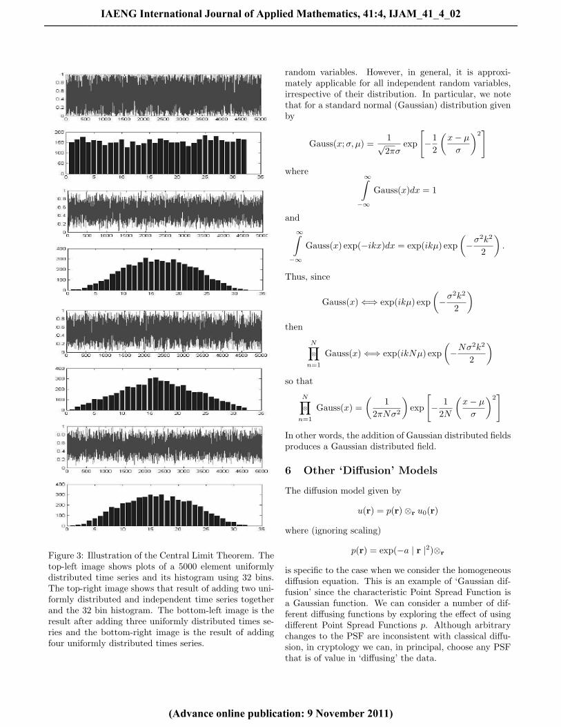
Figure 3: Illustration of the Central Limit Theorem. Thetop-left image shows plots of a 5000 element uniformlydistributed time series and its histogram using 32 bins.The top-right image shows that result of adding two uni-formly distributed and independent time series togetherand the 32 bin histogram. The bottom-left image is theresult after adding three uniformly distributed times se-ries and the bottom-right image is the result of addingfour uniformly distributed times series.

random variables. However, in general, it is approxi-mately applicable for all independent random variables,irrespective of their distribution. In particular, we notethat for a standard normal (Gaussian) distribution givenby

Gauss(x;σ, µ) =1√2πσ

exp

[−1

2

(x− µσ

)2]

where∞∫−∞

Gauss(x)dx = 1

and∞∫−∞

Gauss(x) exp(−ikx)dx = exp(ikµ) exp(−σ

2k2

2

).

Thus, since

Gauss(x)⇐⇒ exp(ikµ) exp(−σ

2k2

2

)then

N∏n=1

⊗ Gauss(x)⇐⇒ exp(ikNµ) exp(−Nσ

2k2

2

)so that

N∏n=1

⊗ Gauss(x) =(

12πNσ2

)exp

[− 1

2N

(x− µσ

)2]

In other words, the addition of Gaussian distributed fieldsproduces a Gaussian distributed field.

6 Other ‘Diffusion’ Models

The diffusion model given by

u(r) = p(r)⊗r u0(r)

where (ignoring scaling)

p(r) = exp(−a | r |2)⊗r

is specific to the case when we consider the homogeneousdiffusion equation. This is an example of ‘Gaussian dif-fusion’ since the characteristic Point Spread Function isa Gaussian function. We can consider a number of dif-ferent diffusing functions by exploring the effect of usingdifferent Point Spread Functions p. Although arbitrarychanges to the PSF are inconsistent with classical diffu-sion, in cryptology we can, in principal, choose any PSFthat is of value in ‘diffusing’ the data.



______________________________________________________________________________________

6.1 Diffusion by Noise

Given the classical diffusion/confusion model of the type

u(r) = p(r)⊗r u0(r) + n(r)

discussed above, we note that both the operator and thefunctional form of p are derived from solving a physicalproblem (using a Green’s function solution) compoundedin a particular PDE - diffusion or wave equation. We canuse this basic model and consider a variety of PSFs asrequired; this include PSFs that are stochastic functions.Noise diffusion involves interchanging the roles of p andn, i.e. replacing p(r) - a deterministic PSF - with n(r) - astochastic function. Thus, noise diffusion is compoundedin the result

u(r) = n(r)⊗r u0(r) + p(r)

oru(r) = n1(r)⊗r u0(r) + n2(r)

where both n1 and n2 are stochastic function which maybe of the same (i.e. have the same PDFs) or of differenttypes (with different PDFs). This form of diffusion is not‘physical’ in the sense that it does not conform to a phys-ical model as defined by the diffusion or wave equation,for example. Here n(r) can be any stochastic function(synthesized or otherwise).

The simplest form of noise diffusion is

u(r) = n(r)⊗r u0(r).

The expected statistical distribution associated with theoutput of noise diffusion process is Gaussian. This canbe shown if we consider u0 to be a strictly deterministicfunction described by a sum of delta functions, equivalentto a binary stream in 1D or a binary image in 2D (discretecases), for example. Thus if

u0(r) =∑i

δn(r− ri)

then

u(r) = n(r)⊗r u0(r) =N∑i=1

n(r− ri).

Now, each function n(r−ri) is just n(r) shifted by ri andwill thus be identically distributed. Hence

Pr[u(r)] = Pr

[N∑i=1

n(r− ri)

]=

N∏i=1

⊗ Pr[n(r)]

and from the Central Limit Theorem, we can expectPr[u(r)] to be normally distributed for large N . In par-ticular, if

Pr[n(r)] =

{1X , | x |≤ X/2;0, otherwise

then

N∏i=1

⊗ Pr[n(r)] '√

6πXN

exp(−6x2/XN).

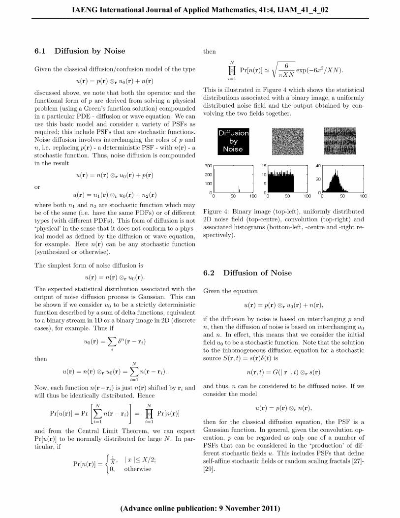
This is illustrated in Figure 4 which shows the statisticaldistributions associated with a binary image, a uniformlydistributed noise field and the output obtained by con-volving the two fields together.

Figure 4: Binary image (top-left), uniformly distributed2D noise field (top-centre), convolution (top-right) andassociated histograms (bottom-left, -centre and -right re-spectively).

6.2 Diffusion of Noise

Given the equation

u(r) = p(r)⊗r u0(r) + n(r),

if the diffusion by noise is based on interchanging p andn, then the diffusion of noise is based on interchanging u0

and n. In effect, this means that we consider the initialfield u0 to be a stochastic function. Note that the solutionto the inhomogeneous diffusion equation for a stochasticsource S(r, t) = s(r)δ(t) is

n(r, t) = G(| r |, t)⊗r s(r)

and thus, n can be considered to be diffused noise. If weconsider the model

u(r) = p(r)⊗r n(r),

then for the classical diffusion equation, the PSF is aGaussian function. In general, given the convolution op-eration, p can be regarded as only one of a number ofPSFs that can be considered in the ‘production’ of dif-ferent stochastic fields u. This includes PSFs that defineself-affine stochastic fields or random scaling fractals [27]-[29].



______________________________________________________________________________________

7 Information and Entropy

Consider a simple linear array such as a deck of eightcards which contains the ace of diamonds for exampleand where we are allowed to ask a series of sequentialquestions as to where in the array the card is. The firstquestion we could ask is in which half of the array doesthe card occur which reduces the number of cards to four.The second question is in which half of the remaining fourcards is the ace of diamonds to be found leaving just twocards and the final question is which card is it. Eachsuccessive question is the same but applied to successivesubdivisions of the deck and in this way we obtain the re-sult in three steps regardless of where the card happensto be in the deck. Each question is a binary choice and inthis example, 3 is the minimum number of binary choiceswhich represents the amount of information required tolocate the card in a particular arrangement. This is thesame as taking the binary logarithm of the number ofpossibilities, since log2 8 = 3. Another way of appreciat-ing this result, is to consider a binary representation ofthe array of cards, i.e. 000,001,010,011,100,101,110,111,which requires three digits or bits to describe any onecard. If the deck contained 16 cards, the informationwould be 4 bits and if it contained 32 cards, the informa-tion would be 5 bits and so on. Thus, in general, for anynumber of possibilities N , the information I for specify-ing a member in such a linear array, is given by

I = − log2N = log2

1N

where the negative sign is introduced to denote that in-formation has to be acquired in order to make the cor-rect choice, i.e. I is negative for all values of N largerthan 1. We can now generalize further by consideringthe case where the number of choices N are subdividedinto subsets of uniform size ni. In this case, the infor-mation needed to specify the membership of a subset isgiven not by N but by N/ni and hence, the informationis given by

Ii = log2 Pi

where Pi = ni/N which is the proportion of the subsets.Finally, if we consider the most general case, where thesubsets are non-uniform in size, then the information willno longer be the same for all subsets. In this case, we canconsider the mean information given by

I =∑i

Pi log2 Pi

which is the Shannon Entropy measure established in hisclassic works on information theory in the 1940s [30]. In-formation, as defined here, is a dimensionless quantity.However, its partner entity in physics has a dimension

called ‘Entropy’ which was first introduced by LudwigBoltzmann as a measure of the dispersal of energy, ina sense, a measure of disorder, just as information is ameasure of order. In fact, Boltzmann’s Entropy concepthas the same mathematical roots as Shannon’s informa-tion concept in terms of computing the probabilities ofsorting objects into bins (a set of N into subsets of sizeni) and in statistical mechanics the Entropy is defined as[31]

E = −k∑i

Pi lnPi

where k is Boltzmann’s constant. Shannon’s and Boltz-mann’s equations are similar. E and I have oppositesigns, but otherwise differ only by their scaling factorsand they convert to one another by E = −(k ln 2)I.Thus, an Entropy unit is equal to −k ln 2 of a bit. InBoltzmann’s equation, the probabilities Pi refer to inter-nal energy levels. In Shannon’s equations Pi are not apriori assigned such specific roles and the expression canbe applied to any physical system to provide a measure oforder. Thus, information becomes a concept equivalent toEntropy and any system can be described in terms of oneor the other. An increase in Entropy implies a decreaseof information and vise versa. This gives rise to the fun-damental conservation law: ˇThe sum of (macroscopic)information change and Entropy change in a given sys-tem is zero.

7.1 Entropy Based Information Extrac-tion

In signal analysis, the Entropy is a measure of the lack ofinformation about the exact information content of thesignal, i.e. the value of fi for a given i. Thus, noisysignals (and data in general) have a larger Entropy. Thegeneral definition for the Entropy of a system E is

E = −∑i

Pi lnPi

where Pi is the probability that the system is in a state i.The negative sign is introduced because the probabilityis a value between 0 and 1 and therefore, lnPi is a valuebetween 0 and −∞, but the Entropy is by definition, apositive value.

An Entropy based approach to the extraction of infor-mation from noise [32] can be designed using an Entropymeasure defined in terms of the data fi (rather than thePDF). A reconstruction for fi is found such that

E = −∑i

fi ln fi



______________________________________________________________________________________

is a maximum which requires that fi > 0∀i. Note thatthe function x lnx has a single local minimum value be-tween 0 and 1 whereas the function −x lnx has a singlelocal maximum value. It is a matter of convention as towhether a criteria of the type

E =∑i

fi ln fi

orE = −

∑i

fi ln fi

is used leading to (strictly speaking) a minimum or max-imum Entropy criterion respectively. In some ways, theterm ‘Maximum Entropy’ is misleading because it impliesthat we are attempting to recover information from noisewith minimum information content and the term ‘Mini-mum Entropy’ conveys a method that is more consistentwith the philosophy of what is being attempted, i.e. torecover useful and unambiguous information from a sig-nal whose information content has been distorted or con-fused by (additive) noise. For example, suppose we inputa binary stream into some time invariant linear system,where f = (...010011011011101...). Then, the input hasan Entropy of zero since 0 ln 0 = 0 and 1 ln 1 = 0. Wecan expect the output of such a system to generate a newarray of values (via the diffusion process) which are thenperturbed (via the confusion process) through additivenoise. The output ui = pi⊗i fi +ni (where it is assumedthat ui > 0∀i and ⊗i denotes the convolution sum overi) will therefore have an Entropy that is greater than 0.Clearly, as the magnitude of the noise increases, so, thevalue of the Entropy increases leading to greater loss ofinformation on the exact state of the input (in terms offi, for some value of i being 0 or 1). With the inverseprocess, we ideally want to recover the input without anybit-errors. In such a hypothetical case, the Entropy of therestoration would be zero. In practice, we approach theproblem in terms of an inverse solution that is based aMinimum Entropy criterion, i.e. find fi such that

E =∑i

fi ln fi

is a minimum or for a continuous field f(r) in n-dimensions, find f such that

E =∫f(r) ln f(r)dnr

is a minimum.

Given that

u(r) = p(r)⊗r f(r) + n(r)

where ⊗r is the convolution integral over r we can write

λ

∫ ([u(r)− p(r)⊗r f(r)]2 − [n(r)]2

)dnr = 0

an equation that holds for any constant λ (the Lagrangemultiplier). We can therefore write the equation for E as

E = −∫f(r) ln f(r)dnr

+λ∫ (

[u(r)− p(r)⊗r f(r)]2 − [n(r)]2)dnr

because the second term on the right hand side is zeroanyway (for all values of λ). Given this equation, ourproblem is to find f such that the Entropy E is a maxi-mum when

∂E

∂f= 0,

i.e. when

−1− ln f(r) + 2λ[u(r)�r p(r)− p(r)⊗r f(r)�r p(r)] = 0

where �r denotes the correlation integral over r. Rear-ranging,

f(r) = exp[−1 + 2λ[u(r)�r p(r)− p(r)⊗r f(r)�r p(r)].

This equation is transcendental in f and as such, requiresthat f is evaluated iteratively, i.e.

[f(r)]n+1 = exp[−1 + 2λ[u(r)�r p(r)

−p(r)⊗r [f(r)]n �r p(r))]

The rate of convergence of this solution is determined bythe value of the Lagrange multiplier given an initial es-timate of f(r), i.e. [f(r)]0. However, the solution canbe linearized by retaining the first two terms (the lin-ear terms) in the series representation of the exponentialfunction leaving us with the following result

f(r) = 2λ[u(r)�r p(r)− p(r)⊗r f(r)�r p(r)].

Using the convolution and correlation theorems, inFourier space, this equation becomes

F (k) = 2λU(k)[P (k)]∗ − 2λ | P (k) |2 F (k)

which after rearranging gives

F (k) =U(k)[P (k)]∗

| P (k) |2 + 12λ

.

so that

f(r) =1

(2π)n

∞∫−∞

[P (k)]∗U(k)| P (k) |2 + 1

2λ

exp(ik · r)dnk.

The cross Entropy or Patterson Entropy uses a criterionin which the Entropy measure

E = −∫dnrf(r) ln

[f(r)w(r)

]



______________________________________________________________________________________

is maximized where w(r) is some weighting functionbased on any available a priori information on f(r). Ifthe calculation above is re-worked using this definition ofthe cross Entropy, then we obtain the result

f(r) = w(r) exp(−1+2λ[u(r)�rp(r)−p(r)⊗rf(r)�rp(r)]).

The cross Entropy method has a synergy with the Wilkin-son test in which a PDF Pn(x) say of a stochastic fieldn(r) is tested against the PDF Pm(x) of a stochastic fieldm(r). A standard test to quantify how close the stochas-tic behaviour of n is to m (the null-hypothesis test) is touse the Chi-squared test in which we compute

χ2 =∫ (

Pn(x)− Pm(x)Pm(x)

)2

dx.

The Wilkinson test uses the metric

E = −∫Pn(x) ln

(Pn(x)Pm(x)

)dx.

7.2 Entropy Conscious Confusion andDiffusion

From the point of view of designing an appropriate sub-stitution cipher, the discussion above clearly dictates thatthe cipher n[i] should be such that the Entropy of the ci-phertext u[i] is a maximum. This requires that a PseudoRandom Number Generation (PRNG) algorithm be de-signed that outputs a number stream whose Entropy is amaximum. There are a wide range of algorithms for gen-erating pseudo random number streams that are continu-ally being developed and improved upon for applicationsto random pattern generation [33] and image encryption[34], for example, and are usually based on some form ofnumerical iteration or ‘round transformation’. However,irrespective of the application, a governing condition inthe design of a PRNG is determined by the InformationEntropy of the stream that is produced. Since the Infor-mation Entropy of the stream is defined as

E =N∑i=1

Pilog2Pi

it is clear that the stream should have a PDF Pi thatyields the largest possible values for E. Figure 5 shows auniformly distributed and a Gaussian distributed randomnumber stream consisting of 3000 elements and the char-acteristic discrete PDFs using 64-bins (i.e. for N = 64).The Information Entropy, which is computed directlyfrom the PDFs using the expression for E given above, isalways greater for the uniformly distributed field. This is

to be expected because, for a uniformly distributed field,there is no bias associated with any particular numericalrange and hence, no likelihood can be associated with aparticular state. Hence, one of the underlying principals

Figure 5: A 3000 element uniformly distributed randomnumber stream (top left) and its 64-bin discrete PDF(top right) with E = 4.1825 and a 3000 element Gaussiandistributed random number stream (bottom left) and its64-bin discrete PDF (bottom right) with E = 3.2678.

associated with the design of a cipher n[i] is that it shouldoutput a uniformly distributed sequence of random num-bers. However, this does not mean that the ciphertextitself will be uniformly distributed since if

u(r) = u0(r) + n(r)

thenPr[u(r)] = Pr[u0(r)]⊗r Pr[n(r)].

This is illustrated in Figure 6 which shows 256-bin his-tograms for an 8-bit ASCII plaintext (the LaTeX file as-sociated with this paper) u0[i], a stream of uniformly dis-tributed integers n[i], 0 ≤ n ≤ 255 and the ciphertextu[i] = u0[i] + n[i]. The spike associate with the plaintexthistogram reflects the ‘character’ that is most likely tooccur in the plaintext of a natural Indo-European lan-guage, i.e. a space with ASCII value 32. Although thedistribution of the ciphertext is broader than the plain-text it is not as broad as the cipher and certainly notuniform. Thus, the Entropy of the ciphertext, althoughlarger than the plaintext (in this example Eu0 = 3.4491and Eu = 5.3200), the Entropy of the ciphertext isstill less that then that of the cipher (in this exampleEn = 5.5302). There are two ways in which this problemcan be solved. The first method is to construct a ciphern with a PDF such that

Pn(x)⊗x Pu0(x) = U(x)



______________________________________________________________________________________

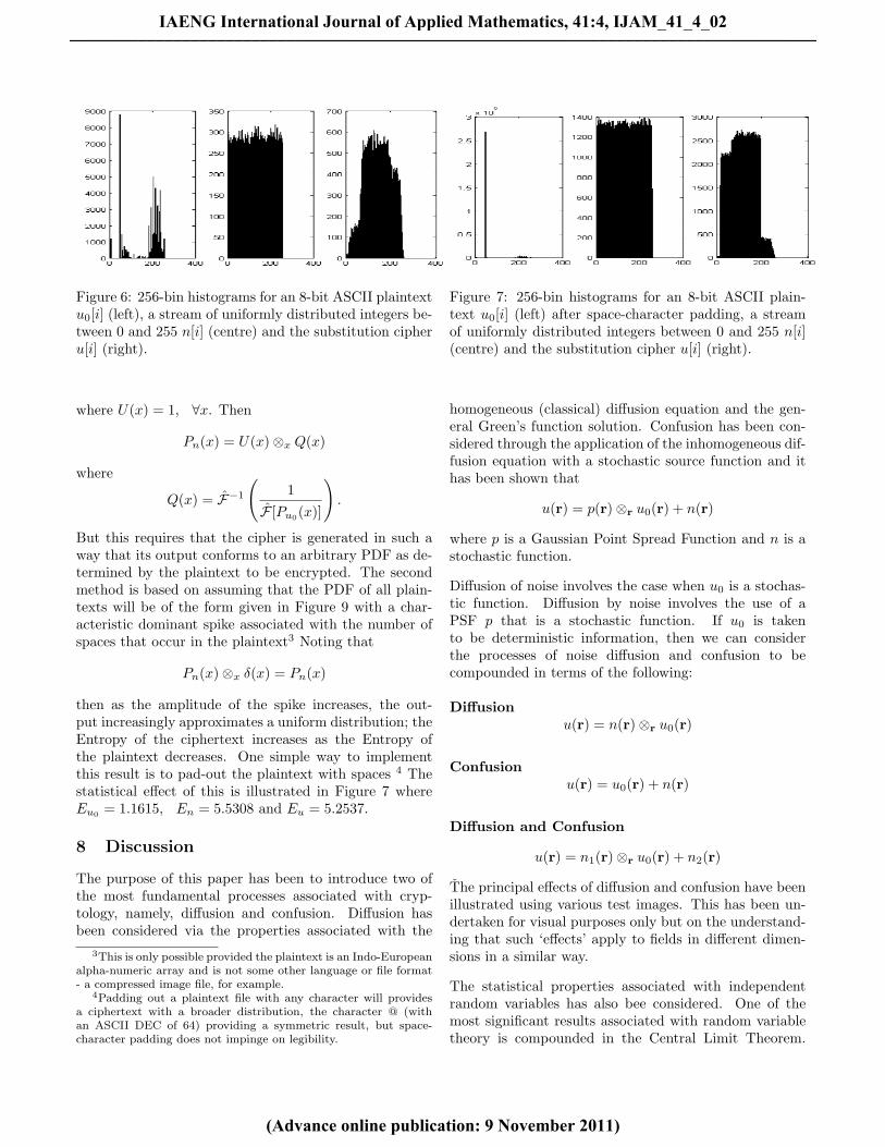
Figure 6: 256-bin histograms for an 8-bit ASCII plaintextu0[i] (left), a stream of uniformly distributed integers be-tween 0 and 255 n[i] (centre) and the substitution cipheru[i] (right).

where U(x) = 1, ∀x. Then

Pn(x) = U(x)⊗x Q(x)

where

Q(x) = F−1

(1

F [Pu0(x)]

).

But this requires that the cipher is generated in such away that its output conforms to an arbitrary PDF as de-termined by the plaintext to be encrypted. The secondmethod is based on assuming that the PDF of all plain-texts will be of the form given in Figure 9 with a char-acteristic dominant spike associated with the number ofspaces that occur in the plaintext3 Noting that

Pn(x)⊗x δ(x) = Pn(x)

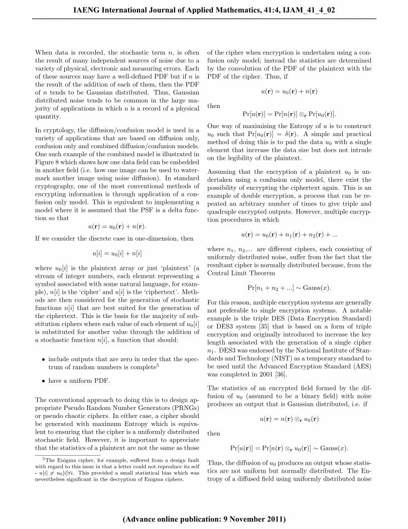
then as the amplitude of the spike increases, the out-put increasingly approximates a uniform distribution; theEntropy of the ciphertext increases as the Entropy ofthe plaintext decreases. One simple way to implementthis result is to pad-out the plaintext with spaces 4 Thestatistical effect of this is illustrated in Figure 7 whereEu0 = 1.1615, En = 5.5308 and Eu = 5.2537.

8 Discussion

The purpose of this paper has been to introduce two ofthe most fundamental processes associated with cryp-tology, namely, diffusion and confusion. Diffusion hasbeen considered via the properties associated with the

3This is only possible provided the plaintext is an Indo-Europeanalpha-numeric array and is not some other language or file format- a compressed image file, for example.

4Padding out a plaintext file with any character will providesa ciphertext with a broader distribution, the character @ (withan ASCII DEC of 64) providing a symmetric result, but space-character padding does not impinge on legibility.

Figure 7: 256-bin histograms for an 8-bit ASCII plain-text u0[i] (left) after space-character padding, a streamof uniformly distributed integers between 0 and 255 n[i](centre) and the substitution cipher u[i] (right).

homogeneous (classical) diffusion equation and the gen-eral Green’s function solution. Confusion has been con-sidered through the application of the inhomogeneous dif-fusion equation with a stochastic source function and ithas been shown that

u(r) = p(r)⊗r u0(r) + n(r)

where p is a Gaussian Point Spread Function and n is astochastic function.

Diffusion of noise involves the case when u0 is a stochas-tic function. Diffusion by noise involves the use of aPSF p that is a stochastic function. If u0 is takento be deterministic information, then we can considerthe processes of noise diffusion and confusion to becompounded in terms of the following:

Diffusionu(r) = n(r)⊗r u0(r)

Confusionu(r) = u0(r) + n(r)

Diffusion and Confusion

u(r) = n1(r)⊗r u0(r) + n2(r)

The principal effects of diffusion and confusion have beenillustrated using various test images. This has been un-dertaken for visual purposes only but on the understand-ing that such ‘effects’ apply to fields in different dimen-sions in a similar way.

The statistical properties associated with independentrandom variables has also bee considered. One of themost significant results associated with random variabletheory is compounded in the Central Limit Theorem.



______________________________________________________________________________________

When data is recorded, the stochastic term n, is oftenthe result of many independent sources of noise due to avariety of physical, electronic and measuring errors. Eachof these sources may have a well-defined PDF but if n isthe result of the addition of each of them, then the PDFof n tends to be Gaussian distributed. Thus, Gaussiandistributed noise tends to be common in the large ma-jority of applications in which u is a record of a physicalquantity.

In cryptology, the diffusion/confusion model is used in avariety of applications that are based on diffusion only,confusion only and combined diffusion/confusion models.One such example of the combined model is illustrated inFigure 8 which shows how one data field can be embeddedin another field (i.e. how one image can be used to water-mark another image using noise diffusion). In standardcryptography, one of the most conventional methods ofencrypting information is through application of a con-fusion only model. This is equivalent to implementing amodel where it is assumed that the PSF is a delta func-tion so that

u(r) = u0(r) + n(r).

If we consider the discrete case in one-dimension, then

u[i] = u0[i] + n[i]

where u0[i] is the plaintext array or just ‘plaintext’ (astream of integer numbers, each element representing asymbol associated with some natural language, for exam-ple), n[i] is the ‘cipher’ and u[i] is the ‘ciphertext’. Meth-ods are then considered for the generation of stochasticfunctions n[i] that are best suited for the generation ofthe ciphertext. This is the basis for the majority of sub-stitution ciphers where each value of each element of u0[i]is substituted for another value through the addition ofa stochastic function n[i], a function that should:

• include outputs that are zero in order that the spec-trum of random numbers is complete5

• have a uniform PDF.

The conventional approach to doing this is to design ap-propriate Pseudo Random Number Generators (PRNGs)or pseudo chaotic ciphers. In either case, a cipher shouldbe generated with maximum Entropy which is equiva-lent to ensuring that the cipher is a uniformly distributedstochastic field. However, it is important to appreciatethat the statistics of a plaintext are not the same as those

5The Enigma cipher, for example, suffered from a design faultwith regard to this issue in that a letter could not reproduce its self- u[i] 6= u0[i]∀i. This provided a small statistical bias which wasnevertheless significant in the decryption of Enigma ciphers.

of the cipher when encryption is undertaken using a con-fusion only model; instead the statistics are determinedby the convolution of the PDF of the plaintext with thePDF of the cipher. Thus, if

u(r) = u0(r) + n(r)

thenPr[u(r)] = Pr[n(r)]⊗r Pr[u0(r)].

One way of maximising the Entropy of u is to constructu0 such that Pr[u0(r)] = δ(r). A simple and practicalmethod of doing this is to pad the data u0 with a singleelement that increase the data size but does not intrudeon the legibility of the plaintext.

Assuming that the encryption of a plaintext u0 is un-dertaken using a confusion only model, there exist thepossibility of encrypting the ciphertext again. This is anexample of double encryption, a process that can be re-peated an arbitrary number of times to give triple andquadruple encrypted outputs. However, multiple encryp-tion procedures in which

u(r) = u0(r) + n1(r) + n2(r) + ...

where n1, n2,... are different ciphers, each consisting ofuniformly distributed noise, suffer from the fact that theresultant cipher is normally distributed because, from theCentral Limit Theorem

Pr[n1 + n2 + ...] ∼ Gauss(x).

For this reason, multiple encryption systems are generallynot preferable to single encryption systems. A notableexample is the triple DES (Data Encryption Standard)or DES3 system [35] that is based on a form of tripleencryption and originally introduced to increase the keylength associated with the generation of a single ciphern1. DES3 was endorsed by the National Institute of Stan-dards and Technology (NIST) as a temporary standard tobe used until the Advanced Encryption Standard (AES)was completed in 2001 [36].

The statistics of an encrypted field formed by the dif-fusion of u0 (assumed to be a binary field) with noiseproduces an output that is Gaussian distributed, i.e. if

u(r) = n(r)⊗r u0(r)

then

Pr[u(r)] = Pr[n(r)⊗r u0(r)] ∼ Gauss(x).

Thus, the diffusion of u0 produces an output whose statis-tics are not uniform but normally distributed. The En-tropy of a diffused field using uniformly distributed noise



______________________________________________________________________________________

is therefore less than the Entropy of a confused field. Itis for this reason, that a process of diffusion should ide-ally be accompanied by a process of confusion when suchprocesses are applied to cryptology in general.

The application of noise diffusion for embedding or water-marking one information field in another is an approachthat has a range of applications including diffusion onlycryptology for applications to low resolution print secu-rity for example which is discussed later on in this work.

Since the diffusion of noise by a deterministic PSF pro-duces an output whose statistics tend to be normallydistributed, such fields are not best suited for encryp-tion. However, this process is important in the design ofstochastic fields that have important properties for thecamouflage of encrypted data. This includes the genera-tion of random fractal fields and the use of methods sucha fractal modulation for covert data communications.

9 Lossy Watermarking Method

In ‘image space’, we consider the plaintext to be an imagep(x, y) of compact support x ∈ [−X,X]; y ∈ [−Y, Y ].Stochastic diffusion is then based on the following results:

Encryption

c(x, y) = m(x, y)⊗x ⊗yp(x, y)

wherem(x, y) = F−1

2 [M(kx, ky)]

and ∀kx, ky

M(kx, ky) =

{N∗(kx,ky)|N(kx,ky)|2 , | N(kx, ky) |6= 0;

N∗(kx, ky), | N(kx, ky) |= 0.

Decryption

p(x, y) = n(x, y)�x �yc(x, y)

Here, kx and ky are the spatial frequencies and F−12 de-

notes the two-dimensional inverse Fourier transform. Fordigital image watermarking, we consider a discrete arraypij , i = 1, 2, ..., I; j = 1, 2, ..., J of size I × J and discreteversions of the operators involved, i.e. application of adiscrete Fourier transform and discrete convolution andcorrelation sums.

If we consider a host image denoted by h(x, y), then weconsider a watermarking method based on the equation

c(x, y) = Rm(x, y)⊗x ⊗yp(x, y) + h(x, y)

where‖m(x, y)⊗x ⊗yp(x, y)‖∞ = 1

and‖h(x, y)‖∞ = 1

By normalising the terms in this way, the coefficient0 ≤ R ≤ 1 can be used to adjust the relative magni-tudes of the terms such that the diffused image m(x, y)⊗x⊗yp(x, y) becomes a perturbation of the ‘host image’(covertext) h(x, y). This provides us with a way of digitalwatermarking one image with another, R being referredto as the ‘watermarking ratio’, a term that is equivalent,in this application, to the standard term ‘Signal-to-Noise’or SNR as used in signal and image analysis. For colourimages, the method can be applied by decomposing theimage into its constituent Red, Green and Blue compo-nents. Stochastic diffusion is then applied to each com-ponent separately and the result combined to produce ancolour composite image.

For applications in image watermarking, stochastic diffu-sion has two principal advantages:

• a stochastic field provides uniform diffusion;

• stochastic fields can be computed using randomnumber generators that depend on a single initialvalue or seed (i.e. a private key).

9.1 Binary Image Watermarking

Watermarking a full grey level or colour image in anothergrey or colour image, respectively, using stochastic diffu-sion leads to two problems: (i) it can yield a degrada-tion in the quality of the reconstruction especially whenR is set to a low value which is required when the hostimage has regions that are homogeneous; (ii) the hostimage can be corrupted by the watermark leading to dis-tortions that are visually apparent. Points (i) and (ii)lead to an optimisation problem with regard to the fi-delity of the watermark and host images in respect of thevalue of the watermark ratio that can be applied whichlimits the type of host images that can be used and thefidelity of the ‘decrypts’. However, if we consider theplaintext image p(x, y) to be of binary form, then theoutput of stochastic diffusion can be binarized to give abinary ciphertext. The rationale for imposing this condi-tion is based on considering a system in which a user isinterested in covertly communicating documents such asconfidential letters and certificates, for example.

If we consider a plaintext image p(x, y) which is a binaryarray, then stochastic diffusion using a pre-conditioned



______________________________________________________________________________________

cipher 0 ≤ m(x, y) ≤ 1 consisting of an array of floatingpoint numbers will generate a floating point output. TheShannon Information Entropy of of any array A(xi, yi)with Probability Mass Function (PMF) p(zi) is given by

I = −∑i=1

p(zi) log2 p(zi)

The information entropy of a binary plaintext image(with PMF consisting of two components whose sum is1) is therefore significantly less than the information en-tropy of the ciphertext image. In other words, for a bi-nary plaintext and a non-binary cipher, the ciphertext isdata redundant. This provides us with the opportunityof binarizing the ciphertext by applying a threshold, i.e.if cb(x, y) is the binary ciphertext, then

cb(x, y) =

{1, c(x, y) > T

0, c(x, y) ≤ T(2)

where 0 ≤ c(x, y) ≤ 1∀x, y. A digital binary ciphertextimage cb(xi, yj) where

cb(xi, yi) =

{1, or0, for any xi, yj

can then be used to watermark an 8-bit host imageh(x, y), h ∈ [0, 255] by replacing the lowest 1-bit layerwith cb(xi, xj). To recover this information, the 1-bitlayer is extracted from the image and the result corre-lated with the digital cipher n(xi, yj). Note that theoriginal floating point cipher n is required to recover theplaintext image and that the binary watermark can nottherefore be attacked on an exhaustive XOR basis usingtrial binary ciphers. Thus, binarization of a stochasticallydiffused data field is entirely irreversible.

9.2 Statistical Analysis

The expected statistical distribution associated withstochastic diffusion is Gaussian. This can be shown ifwe consider a binary plaintext image pb(x, y) to be de-scribed by a sum of N delta functions where each deltafunction describes the location of a non-zero bit at coor-dinates (xi, yj). Thus if

pb(x, y) =N∑i=1

N∑j=1

δ(x− xi)δ(y − yj)

thenc(x, y) = m(x, y)⊗x ⊗yp(x, y)

=N∑i=1

N∑j=1

m(x− xi, y − yj).

Each function m(x − xi, y − yj) is just m(x, y) shiftedby xi, yj and will thus be identically distributed. Hence,from the Central Limit Theorem

Pr[c(x, y)] = Pr

N∑i=1

N∑j=1

m(x− xi, y − yj)

=

N∏i=1

⊗ Pr[m(x, y)] ≡ Pr[m(x, y)]⊗x⊗yPr[m(x, y)]⊗x⊗y...

∼ Gaussian(z), N →∞where Pr denotes the Probability Density Function. Wecan thus expect Pr[c(x, y)] to be normally distributed andfor m(x, y) ∈ [0, 1]∀x, y the mode of the distribution willbe of the order of 0.5. This result provides a value forthe threshold T in equation (2) which for 0 ≤ c(x, y) ≤ 1is 0.5 (theoretically). Note that if n(x, y) is uniformlydistributed and thereby represents δ-uncorrelated noisethen both the complex spectrum N∗ and power spectrum| N |2 will also be δ-uncorrelated and since

m(x, y) = F−12

[N∗(kx, ky)| N(kx, ky) |2

]Pr[m(x, y)] will be uniformly distributed. Also note thatthe application of a threshold which is given by the modeof the Gaussian distribution, guarantees that there is nostatistical bias associated with any bit in the binary out-put, at least, on a theoretical basis. On a practical ba-sis, the needs to be computed directly by calculating themode from the histogram of the cipher and that bit equal-ization can not be guaranteed as it will depend on: (i)the size of the images used; (ii) the number of bins usedto compute the histogram.

9.3 Principal Algorithms

The principal algorithms associated with the applicationof stochastic diffusion for watermarking with ciphers areas follows:

Algorithm I: Encryption and Watermarking Al-gorithm

Step 1: Read the binary plaintext image from a file andcompute the size I × J of the image.

Step 2: Compute a cipher of size I × J using a privatekey and pre-condition the result.

Step 3: Convolve the binary plaintext image with thepre-conditioned cipher and normalise the output.



______________________________________________________________________________________

Step 4: Binarize the output obtained in Step 3 using athreshold based on computing the mode of the Gaussiandistributed ciphertext.

Step 5: Insert the binary output obtained in Step 4 intothe lowest 1-bit layer of the host image and write theresult to a file.

The following points should be noted:

(i) The host image is taken to be an 8-bit or higher greylevel image which must ideally be the same size as theplaintext image or else resized accordingly. However, inresembling the host image, its proportions should be thesame so that the stegotext image does not appear to bea distorted version of the covertext image. For this pur-pose, a library of host images should be developed whosedimensions are set according to a predetermined appli-cation where the dimensions of the plaintext image areknown.

(ii) Pre-conditioning the cipher and the convolution pro-cesses are undertaken using a Discrete Fourier Transform(DFT).

(iii) The output given in Step 3 will include negative float-ing point numbers upon taking the real component of acomplex array. The array must be rectified by adding thelargest negative value in the output array to the same ar-ray before normalisation.

(iv) For colour host images, the binary ciphertext can beinserted in to one or all of the RGB components. Thisprovides the facility for watermarking the host image withthree binary ciphertexts (obtained from three separatebinary documents, for example) into a full colour image.In each case, a different key can be used.

(v) The binary plaintext image should have homogeneousmargins in order to minimise the effects of ringing due to‘edge-effects’ when processing the data in the spectraldomain.

Algorithm II: Decryption Algorithm

Step 1: Read the watermarked image from a file andextract the lowest 1-bit layer from the image.

Step 2: Regenerate the (non-preconditioned) cipher us-ing the same key used in Algorithm I.

Step 3: Correlate the cipher with the input obtained inStep 1 and normalise the result.

Step 4: Quantize and format the output from Step 3and write to a file.

The following points should be noted:

(i) The correlation operation should be undertaken usinga DFT.

(ii) For colour images, the data is decomposed into eachRGB component and each 1-bit layer is extracted and cor-related with the appropriate cipher, i.e. the same cipheror three ciphers relating to three private keys respectively.

(iii) The output obtained in Step 3 has a low dynamicrange and therefore requires to be quantized into an 8-bitimage based on floating point numbers within the rangemax(array)-min(array).

9.4 StegoText

StegoText is a prototype tool designed using MATLAB toexamine the applications to which stochastic diffusion canbe used. A demonstration version of the system is avail-able at http://eleceng.dit.ie/arg/downloads/Stegocryptwhich has been designed with a simple Graphical UserInterface as shown in Figure 8 whose use is summarisedin the following table:

Encryption Mode Decryption ModeInputs: Inputs:Plaintext image Stegotext imageCovertext image Private key (PIN)Private Key (PIN)Output: Output:Watermarked image Decrypted watermarkOperation: Operation:Encrypt by clicking on Decrypt by clicking onbuttom E (for Encrypt) button D (for Dycrypt)

The PIN (Personal Identity Number) can be an numer-ical string with upto 16 elements. In principal, any ex-isting encryption algorithm, application or system canbe used to generate the cipher required by StegoText byencrypting an image composed of random noise. The out-put is then needs to be converted into a decimal integerarray and the result normalised as required, i.e. depend-ing on the format of the output that is produced by a



______________________________________________________________________________________

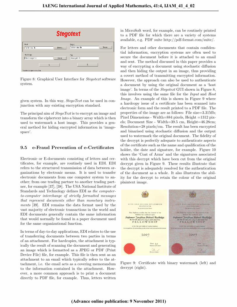
Figure 8: Graphical User Interface for Stegotext softwaresystem.

given system. In this way, StegoText can be used in con-junction with any existing encryption standard.

The principal aim of StegoText is to encrypt an image andtransform the ciphertext into a binary array which is thenused to watermark a host image. This provides a gen-eral method for hiding encrypted information in ‘image-space’.

9.5 e-Fraud Prevention of e-Certificates

Electronic or E-documents consisting of letters and cer-tificates, for example, are routinely used in EDI. EDIrefers to the structured transmission of data between or-ganizations by electronic means. It is used to transferelectronic documents from one computer system to an-other; from one trading partner to another trading part-ner, for example [37], [38]. The USA National Institute ofStandards and Technology defines EDI as the computer-to-computer interchange of strictly formatted messagesthat represent documents other than monetary instru-ments [39]. EDI remains the data format used by thevast majority of electronic transactions in the world andEDI documents generally contain the same informationthat would normally be found in a paper document usedfor the same organizational function.

In terms of day-to-day applications, EDI relates to the useof transferring documents between two parties in termsof an attachment. For hardcopies, the attachment is typ-ically the result of scanning the document and generatingan image which is formatted as a JPEG or PDF (PrintDevice File) file, for example. This file is then sent as anattachment to an email which typically refers to the at-tachment, i.e. the email acts as a covering memorandumto the information contained in the attachment. How-ever, a more common approach is to print a documentdirectly to PDF file, for example. Thus, letters written

in MicroSoft word, for example, can be routinely printedto a PDF file for which there are a variety of systemsavailable, e.g. PDF suite http://pdf-format.com/suite/.

For letters and other documents that contain confiden-tial information, encryption systems are often used tosecure the document before it is attached to an emailand sent. The method discussed in this paper provides away of encrypting a document using stochastic diffusionand then hiding the output in an image, thus providinga covert method of transmitting encrypted information.However, the approach can also be used to authenticatea document by using the original document as a ‘hostimage’. In terms of the Stegotext GUI shown in Figure 8,this involves using the same file for the Input and HostImage. An example of this is shown in Figure 9 wherea hardcopy issue of a certificate has been scanned intoelectronic form and the result printed to a PDF file. Theproperties of the image are as follows: File size=3.31Mb;Pixel Dimensions - Width=884 pixels, Height =1312 pix-els; Document Size - Width=39.5 cm, Height=46.28cm;Resolution=28 pixels/cm. The result has been encryptedand binarised using stochastic diffusion and the outputused to watermark the original document. The fidelity ofthe decrypt is perfectly adequate to authenticate aspectsof the certificate such as the name and qualification of theholder, the date and signature, for example. Figure 10shows the ‘Coat of Arms’ and the signatures associatedwith this decrypt which have been cut from the originaldecrypt given in Figure 9. These results illustrate thatthe decrypt is adequately resolved for the authenticationof the document as a whole. It also illustrates the abil-ity for the decrypt to retain the colour of the originalplaintext image.

Figure 9: Certificate with binary watermark (left) anddecrypt (right).



______________________________________________________________________________________

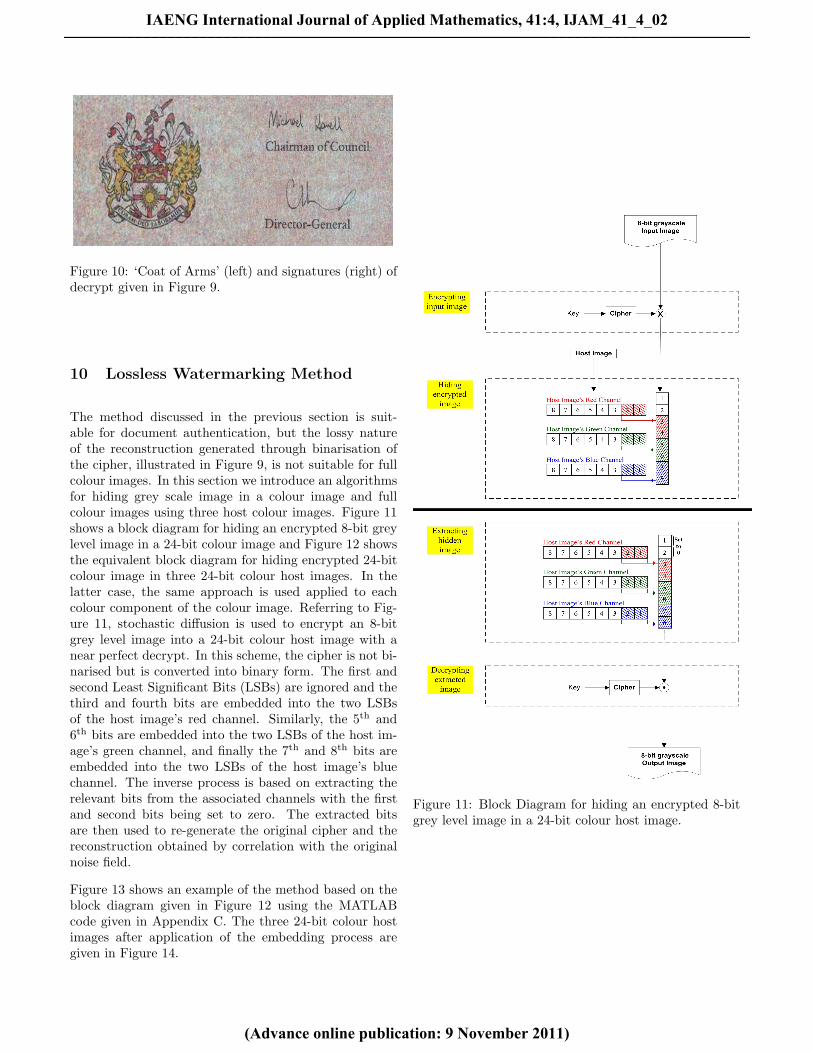
Figure 10: ‘Coat of Arms’ (left) and signatures (right) ofdecrypt given in Figure 9.

10 Lossless Watermarking Method

The method discussed in the previous section is suit-able for document authentication, but the lossy natureof the reconstruction generated through binarisation ofthe cipher, illustrated in Figure 9, is not suitable for fullcolour images. In this section we introduce an algorithmsfor hiding grey scale image in a colour image and fullcolour images using three host colour images. Figure 11shows a block diagram for hiding an encrypted 8-bit greylevel image in a 24-bit colour image and Figure 12 showsthe equivalent block diagram for hiding encrypted 24-bitcolour image in three 24-bit colour host images. In thelatter case, the same approach is used applied to eachcolour component of the colour image. Referring to Fig-ure 11, stochastic diffusion is used to encrypt an 8-bitgrey level image into a 24-bit colour host image with anear perfect decrypt. In this scheme, the cipher is not bi-narised but is converted into binary form. The first andsecond Least Significant Bits (LSBs) are ignored and thethird and fourth bits are embedded into the two LSBsof the host image’s red channel. Similarly, the 5th and6th bits are embedded into the two LSBs of the host im-age’s green channel, and finally the 7th and 8th bits areembedded into the two LSBs of the host image’s bluechannel. The inverse process is based on extracting therelevant bits from the associated channels with the firstand second bits being set to zero. The extracted bitsare then used to re-generate the original cipher and thereconstruction obtained by correlation with the originalnoise field.

Figure 13 shows an example of the method based on theblock diagram given in Figure 12 using the MATLABcode given in Appendix C. The three 24-bit colour hostimages after application of the embedding process aregiven in Figure 14.

Figure 11: Block Diagram for hiding an encrypted 8-bitgrey level image in a 24-bit colour host image.



______________________________________________________________________________________

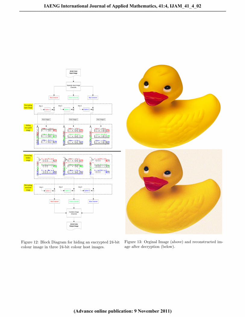
24-bit Color

Input Image

Separate Input Image

Channels

Green Channel Blue ChannelRed Channel

Cipher-1 x

Key-1

Cipher-2 x

Key-2

Cipher-3 x

Key-3

Host Image-1 Host Image-2 Host Image-3

24-bit Color

Output Image

Combine Image

Channels

Green Channel Blue ChannelRed Channel

Cipher-1

Key-1

Cipher-2

Key-2

Cipher-3

Key-3

Encrypting

input image

Decrypting

extracted

image

Hiding

encrypted

image

Extracting

hidden

image

Figure 12: Block Diagram for hiding an encrypted 24-bitcolour image in three 24-bit colour host images.

Figure 13: Orginal Image (above) and reconstructed im-age after decryption (below).



______________________________________________________________________________________

Figure 14: Host images used to hide the image given inFigure 13 after embedding the ciphers.

11 Conclusions

This paper has focused on the application of stochasticdiffusion for transmitting e-documents and digital imagesover the internet in such a way that encrypted informa-tion can be communicated covertly and the informationauthenticated. The use of the Internet to transfer docu-ments as image attachments has and continues to growrapidly. It is for this ‘market’ that the approach reportedin this paper has been developed. Inserting a binary wa-termark into a host image obtained by binarizing a float-ing point ciphertext (as discussed in Section 9) providesa cryptographically secure solution. This is because bi-narization is an entirely one-way process. Thus, althoughthe watermark may be removed from the covertext im-age, it can not be decrypted without the recipient havingaccess to the correct cryptographically secure algorithmand key. The approach discussed in Section 9.4 and theStegoText system currently available has a range of ap-plication for e-document authentication. For example,many institutes such as universities still issue ‘paper cer-tificates’ to their graduates. These certificates are thenscanned and sent as attachments along with a CV andcovering letter when applying for a job. It is at this pointthat the certificate may be counterfeited and, for this rea-son, some establishments still demand originals to be sub-mitted. StegoText provides the facility to issue electroniccertificates (in addition or in substitution to a hardcopy)which can then be authenticated as discussed in Section9.4. By including a serial number on each certificate (aCertificate Identity Number) which represents a ‘publickey’, the document can be submitted to the authoritythat issued the certificate for authentication, for whichan online service can be established as required subjectto any regulation of investigatory powers e.g. [40].

In this paper, the method of stochastic diffusion has beenextended to hide 24-bit colour images in a set of three24-bit colour images. This provides a lossless methodof encrypting and covertly communicating 24-bit colourimages over the Internet as required and as illustrated inSection 10. The applications to which stochastic diffusioncan be applied are numerous and, coupled with appropri-ate key-exchange protocols, provides a generic method ofencrypting and hiding digital image information.

Appendix A: Inverse Diffusion

Suppose we consider the homogeneous diffusion problemdefined by the equation

D∇2u(r, t)− ∂

∂tu(r, t) = 0, u(r, 0) = u0(r)



______________________________________________________________________________________

with the solution

u(r, τ) =1DG(| r |, t)⊗r u0(r), t > 0.

If we record a diffused field u after some time t = T , is itpossible to reconstruct the field at time t = 0, i.e. to solvethe inverse problem or de-diffuse the field measured? Wecan express u(r, 0) in terms of u(r, T ) using the Taylorseries

u0(r) ≡ u(r, 0) = u(r, T )+∞∑n=1

(−1)n

n!Tn[∂n

∂tnu(r, t)

]t=T

.

Now, from the diffusion equation

∂2u

∂t2= D∇2 ∂u

∂t= D2∇4u,

∂3u

∂t3= D∇2 ∂

2u

∂t2= D3∇6u

and so on. Thus, in general we can write[∂n

∂tnu(r, t)

]t=T

= Dn∇2nu(x, y, T ).

Substituting this result into the series for u0 given above,we obtain

u0(r) = u(r, T ) +∞∑n=1

(−1)n

n!(DT )n∇2nu(r, T ).

For a time-independent source function S(r) the equiva-lent solution to the equation

D∇2u(r, t)− ∂

∂tu(r, t) = −− S(r), u(r, 0) = u0(r)

is then given byu0(r) = u(r, T )

+∞∑n=1

(−1)n

n![(DT )n∇2nu(r, T ) +D−1∇2n−2S(r)]

Appendix B: Proof by Induction of theCentral Limit Theorem for a UniformlyDistributed Stochastic Function

We consider the effect of applying multiple convolutionsof the uniform distribution

P (x) =

{1X , | x |≤ X/2;0, otherwise

and show that

N∏n=1

⊗ Pn(x) ≡ P1(x)⊗x P2(x)⊗x ...⊗x PN (x)

'√

6πN

exp(−6x2/XN)

where Pn(x) = P (x), ∀n and N is large. This result isbased on considering the effect of multiple convolutionsin Fourier space (through application of the convolutiontheorem) and then working with a series representationof the result.

The Fourier transform of P (x) is given by

P (k) =

∞∫−∞

P (x) exp(−ikx)dx

=

X/2∫−X/2

1X

exp(−ikx)dx = sinc(kX/2)

where sinc(x) = sin(x)/x - the ‘sinc’ function. Thus,

P (x)⇐⇒ sinc(kX/2)

where ⇐⇒ denotes transformation into Fourier space,and from the convolution theorem in follows that

Q(x) =N∏n=1

⊗ Pn(x)⇐⇒ sincN (kX/2).

Using the series expansion of the sin function for an ar-bitrary constant α,

sinc(αk)

=1αk

(αk − 1

3!(αk)3 +

15!

(αk)5 − 17!

(αk)7 + . . .

)= 1− 1

3!(αk)2 +

15!

(αk)4 − 17!

(αk)6 + . . .

The N th power of sinc(αk) can be written in terms of abinomial expansion giving

sincN (αk) =(

1− 13!

(αk)2 +15!

(αk)4 − 17!

(αk)6 + . . .

)N

= 1−N(

13!

(αk)2 − 15!

(αk)4 +17!

(αk)6 − . . .)

+N(N − 1)

2!

(13!

(αk)2 − 15!

(αk)4 +17!

(αk)6 − . . .)2

−N(N − 1)(N − 2)3!

×(

13!

(αk)2 − 15!

(αk)4 +17!

(αk)6 − . . .)3

+ . . .

= 1−N α2k2

3!+N

α4k4

5!− kα

6k6

7!− . . .



______________________________________________________________________________________

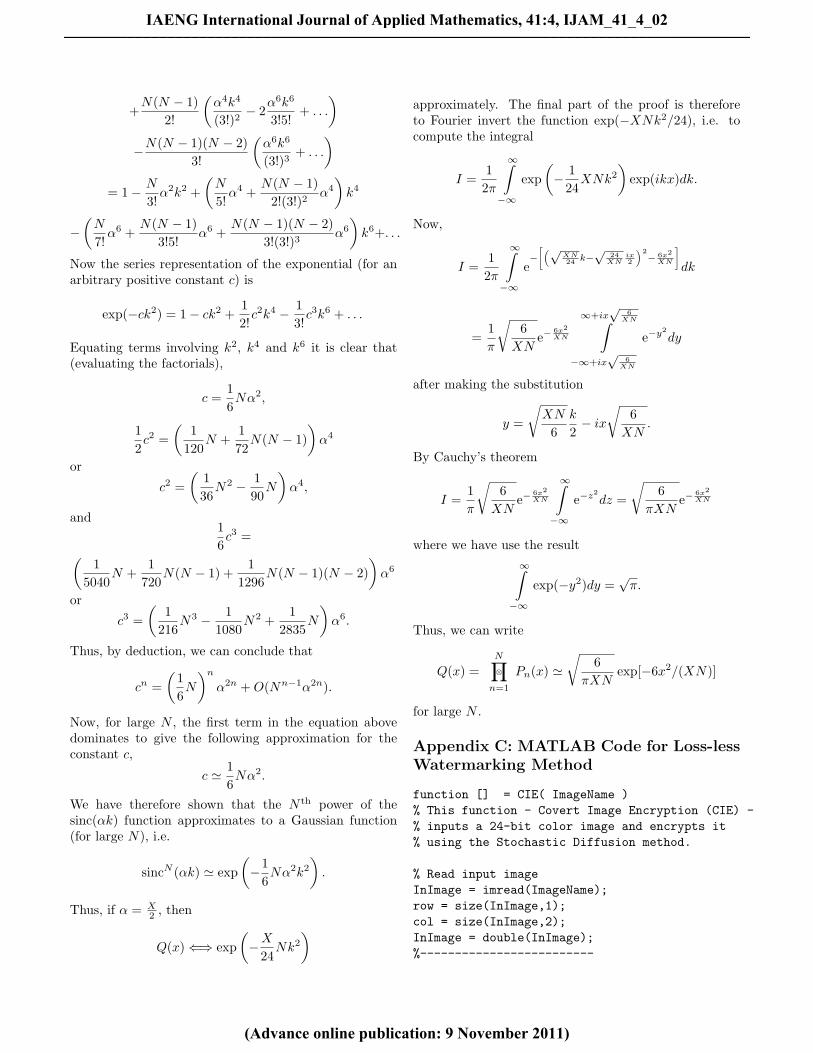
+N(N − 1)

2!

(α4k4

(3!)2− 2

α6k6

3!5!+ . . .

)−N(N − 1)(N − 2)

3!

(α6k6

(3!)3+ . . .

)= 1− N

3!α2k2 +

(N

5!α4 +

N(N − 1)2!(3!)2

α4

)k4

−(N

7!α6 +

N(N − 1)3!5!

α6 +N(N − 1)(N − 2)

3!(3!)3α6

)k6+. . .

Now the series representation of the exponential (for anarbitrary positive constant c) is

exp(−ck2) = 1− ck2 +12!c2k4 − 1

3!c3k6 + . . .

Equating terms involving k2, k4 and k6 it is clear that(evaluating the factorials),

c =16Nα2,

12c2 =

(1

120N +

172N(N − 1)

)α4

or

c2 =(

136N2 − 1

90N

)α4,

and16c3 =(

15040

N +1

720N(N − 1) +

11296

N(N − 1)(N − 2))α6

or

c3 =(

1216

N3 − 11080

N2 +1

2835N

)α6.

Thus, by deduction, we can conclude that

cn =(

16N

)nα2n +O(Nn−1α2n).

Now, for large N , the first term in the equation abovedominates to give the following approximation for theconstant c,

c ' 16Nα2.

We have therefore shown that the N th power of thesinc(αk) function approximates to a Gaussian function(for large N), i.e.

sincN (αk) ' exp(−1

6Nα2k2

).

Thus, if α = X2 , then

Q(x)⇐⇒ exp(−X

24Nk2

)

approximately. The final part of the proof is thereforeto Fourier invert the function exp(−XNk2/24), i.e. tocompute the integral

I =1

2π

∞∫−∞

exp(− 1

24XNk2

)exp(ikx)dk.

Now,

I =1

2π

∞∫−∞

e−[(√

XN24 k−

√24

XNix2

)2− 6x2

XN

]dk

=1π

√6

XNe−

6x2XN

∞+ix√

6XN∫

−∞+ix√

6XN

e−y2dy

after making the substitution

y =

√XN

6k

2− ix

√6

XN.

By Cauchy’s theorem

I =1π

√6

XNe−

6x2XN

∞∫−∞

e−z2dz =

√6

πXNe−

6x2XN

where we have use the result∞∫−∞

exp(−y2)dy =√π.

Thus, we can write

Q(x) =N∏n=1

⊗ Pn(x) '√

6πXN

exp[−6x2/(XN)]

for large N .

Appendix C: MATLAB Code for Loss-lessWatermarking Method

function [] = CIE( ImageName )% This function - Covert Image Encryption (CIE) -% inputs a 24-bit color image and encrypts it% using the Stochastic Diffusion method.

% Read input imageInImage = imread(ImageName);row = size(InImage,1);col = size(InImage,2);InImage = double(InImage);%-------------------------



______________________________________________________________________________________

% Generate the noise field% using Matlab’s rand functionNoiseImageR = rand(row,col);NoiseImageG = rand(row,col);NoiseImageB = rand(row,col);

NR = NoiseImageR;NG = NoiseImageG;NB = NoiseImageB;% -------------------------

% Convolve the input image with the% noise image using a 2D FFT% with pre-conditioningmR = PreCondition(NoiseImageR);mG = PreCondition(NoiseImageG);mB = PreCondition(NoiseImageB);% -----------------------------% Encrypt the Red ChannelCR=ifft2(fft2(mR).*fft2(InImage(:,:,1)) );% Encrypt the Green Channel.CG=ifft2(fft2(mG).*fft2(InImage(:,:,2)) );% Encrypt the Blue ChannelCB=ifft2(fft2(mB).*fft2(InImage(:,:,3)) );

% Normalize Cipher Images to range 0:255.CR = Normalize(CR) .* 255;CG = Normalize(CG) .* 255;CB = Normalize(CB) .* 255;% ------------------------CR = uint8(CR);CG = uint8(CG);CB = uint8(CB);% ------------------------

% Embed cipher images into three% named cover images:%% cover1.bmp% cover2.bmp% cover3.bmp

% Embed red channel cipher into cover image 1CoverImage1 = imread(’cover1.bmp’);CoverImage1 = imresize(CoverImage1 , [row col]);figure(1);subplot(1,2,1), imshow(CoverImage1),title(’Cover Image1 before embedding’);for i = 1 : size(CoverImage1,1)

for j = 1 : size(CoverImage1,2)

CoverImage1(i,j,1) =bitand( CoverImage1(i,j,1) , 252 );

CoverImage1(i,j,1) =bitor( CoverImage1(i,j,1),bitand(bitshift(CR(i,j),-2),3) );


CoverImage1(i,j,2) =bitor( CoverImage1(i,j,2),bitand(bitshift(CR(i,j),-4),3) );

CoverImage1(i,j,3) =bitand( CoverImage1(i,j,3) , 252 );CoverImage1(i,j,3) =bitor( CoverImage1(i,j,3),bitand(bitshift(CR(i,j),-6),3));

endendsubplot(1,2,2), imshow(CoverImage1),title(’Cover Image1 after Embedding’);% -----------------------------------% Embed green channel cipher into Cover Image 2CoverImage2 = imread(’cover2.bmp’);CoverImage2 = imresize(CoverImage2 , [row col]);figure(2);subplot(1,2,1), imshow(CoverImage2),title(’Cover Image2 before Embedding’);

for i = 1 : size(CoverImage2,1)for j = 1 : size(CoverImage2,2)

CoverImage2(i,j,1) =bitand( CoverImage2(i,j,1) , 252 );CoverImage2(i,j,1) =bitor( CoverImage2(i,j,1),bitand(bitshift(CG(i,j),-2),3) );

CoverImage2(i,j,2) =bitand( CoverImage2(i,j,2) , 252 );CoverImage2(i,j,2) =bitor( CoverImage2(i,j,2),bitand(bitshift(CG(i,j),-4),3) );

CoverImage2(i,j,3) =bitand( CoverImage2(i,j,3) , 252 );CoverImage2(i,j,3) =bitor( CoverImage2(i,j,3),bitand(bitshift(CG(i,j),-6),3));

endendsubplot(1,2,2), imshow(CoverImage2),



______________________________________________________________________________________

title(’Cover Image2 after Embedding’);% ------------------------------------% Embed blue channel cipher into Cover Image 3CoverImage3 = imread(’cover3.bmp’);CoverImage3 = imresize(CoverImage3 , [row col]);figure(3);subplot(1,2,1), imshow(CoverImage3),title(’Cover Image3 before Embedding’);

for i = 1 : size(CoverImage3,1)for j = 1 : size(CoverImage3,2)


CoverImage3(i,j,1) =bitor( CoverImage3(i,j,1),bitand(bitshift(CB(i,j),-2),3) );

CoverImage3(i,j,2) =bitand( CoverImage3(i,j,2) , 252 );CoverImage3(i,j,2) =bitor( CoverImage3(i,j,2),bitand(bitshift(CB(i,j),-4),3) );

CoverImage3(i,j,3) =bitand( CoverImage3(i,j,3) , 252 );CoverImage3(i,j,3) =bitor( CoverImage3(i,j,3),bitand(bitshift(CB(i,j),-6),3));

endendsubplot(1,2,2), imshow(CoverImage3),title(’Cover Image3 after Embedding’);% ------------------------------------

% Extract the hidden ciphers from cover images% Extract red channel cipher from cover image 1for i = 1 : size(CoverImage1,1)


R = bitand( CoverImage1(i,j,1), 3);G = bitand( CoverImage1(i,j,2), 3);B = bitand( CoverImage1(i,j,3), 3);ExImageR(i,j) = bitor( bitor(bitshift(R,2),bitshift(G,4)),bitshift(B,6) );

endendExImageR = uint8(ExImageR);% -------------------------%

% Extract green channel cipher% from cover image 2for i = 1 : size(CoverImage2,1)


R = bitand( CoverImage2(i,j,1), 3);G = bitand( CoverImage2(i,j,2), 3);B = bitand( CoverImage2(i,j,3), 3);ExImageG(i,j) = bitor( bitor(bitshift(R,2),bitshift(G,4)),bitshift(B,6) );

endendExImageG = uint8(ExImageG);% -------------------------%% Extract blue channel cipher% from cover image 3for i = 1 : size(CoverImage3,1)


R = bitand( CoverImage3(i,j,1), 3);G = bitand( CoverImage3(i,j,2), 3);B = bitand( CoverImage3(i,j,3), 3);ExImageB(i,j) = bitor( bitor(bitshift(R,2),bitshift(G,4)),bitshift(B,6) );

endendExImageB = uint8(ExImageB);% -------------------------

% Correlate the Extracted ciphers with the% noise field using a 2D FFTExImageR = double(ExImageR);ExImageG = double(ExImageG);ExImageB = double(ExImageB);

PlainImR =ifft2( conj(fft2(NR)) .* fft2(ExImageR) );

PlainImG =ifft2( conj(fft2(NG)) .* fft2(ExImageG) );

PlainImB =ifft2( conj(fft2(NB)) .* fft2(ExImageB) );

% Normalize images to raneg 0:255PlainImR = Normalize(PlainImR) .* 255;PlainImG = Normalize(PlainImG) .* 255;PlainImB = Normalize(PlainImB) .* 255;%-------------------------------------



______________________________________________________________________________________

Result(:,:,1) = PlainImR;Result(:,:,2) = PlainImG;Result(:,:,3) = PlainImB;Result = uint8(Result);imwrite(Result,’Output_Color.bmp’);

figure(4);subplot(1,2,1), imshow(uint8(InImage)),title(’Input Image before Encryption’);

subplot(1,2,2), imshow(Result),title(’Output Image after Decryption’);

end

%--------------------------------------

function [ x ] = Normalize( mat )% Function to normalise images

MAX = max(mat(:)); MIN = min(mat(:));

for i = 1:size(mat,1)for j = 1:size(mat,2)x(i,j) = ((mat(i,j) - MIN )/(MAX - MIN));end

end

return;end

%-----------------------------------

function [ m ] = PreCondition( arr )% Pre-conditioning function

arrF = fft2(arr);for i = 1:size(arrF,1)

for j = 1:size(arrF,2)if abs(arrF(i,j)) == 0

M(i,j) = arrF(i,j);else

M(i,j)=arrF(i,j)/(abs(arrF(i,j))*abs(arrF(i,j)));

endend

endm = ifft2(M);

return;end

Acknowledgments

The authors are grateful for the support of the ScienceFoundation Ireland.

References

[1] Xiaolu, Li., Zhi, Qi., Zhiqiang, Yang, and Jun,Kong., “A Novel Hidden Transmission of BiometricImages Base on Choas and Image Content”, First In-ternational Workshop on Education Technology andComputer Science, 2009

[2] Jun, Kong., Hongru, Jia., Xiaolu. Li., and Zhi,Qi., “A Novel Content-based Information HidingScheme”, International Conference on ComputerEngineering and Technology, 2009

[3] Che-Wei, Lee and Wen-Hasiang, Tsai, “A NewSteganographic Method Based on Information Shar-ing via PNG Images”, IEEE transactions, 2010.

[4] Chen Uuefen, Lin Junhuan, Zhang Shiqing, andChen Caiming, “Double Random Scrambling Algo-rithm Based on Subblocks for Image Hiding”, Inter-national Conference on Computer and Communica-tion Technologies in Agriculture Engineering, 2010.

[5] Ptitsyn, N. V., Blackledge, J. M. and Chernenky V.M., “Deterministic Chaos in Digital Cryptography”,Proceedings of the First IMA Conference on Frac-tal Geometry: Mathematical Methods, Algorithmsand Applications (Eds. J M Blackledge, A K Evansand M Turner), Horwood Publishing Series in Math-ematics and Applications, pp. 189-222, 2002

[6] Ptitsyn, N. V., Deterministic Chaos if Digital Cryp-tography, PhD Thesis, De Montfort University, 2003.

[7] Webster, A. G., Partial Differential Equations ofMathematical Physics, Stechert, 1933.

[8] Morse, P. M. and Feshbach, H., Methods of Theoret-ical Physics, McGraw-Hill, 1953.

[9] Butkov, E., Mathematical Physics, Addison-Wesley,1973.

[10] Evans, G. A., Blackledge, J. M. and Yardley, P., An-alytical Solutions to Partial Differential Equations,Springer, 1999.

[11] Roach, G. F., Green’s Functions (Introductory The-ory with Applications), Van Nostrand Reihold, 1970.



______________________________________________________________________________________

[12] Stakgold, I., Green’s Functions and Boundary ValueProblems, Wiley, 1979.

[13] Dirac, P. A. M., The Principles of Quantum Me-chanics, Oxford University Press, 1947.

[14] Hoskins, R. F., The Delta Function, Horwood Pub-lishing, 1999.

[15] Hoskins, R. G. and Sousa Pinto, J., Theories of Gen-eralised Functions: Distributions, Ultradistributionsand Other Generalised Functions, Horwood, 2005.

[16] Watson, E. J., Laplace Transforms and Applications,Van Nostrand Reinhold, 1981.

[17] Papoulis, A., The Fourier Integral and its Applica-tions, McGraw-Hill, 1962.

[18] Bracewell, R. N., The Fourier Transform and its Ap-plications, McGraw-Hill, 1978.

[19] Ferrers, N. M. (Ed.), Mathematical Papers of GeorgeGreen, Chelsea, 1970.

[20] Wadsworth, G. P. and Bryan, J. G., Introductionto Probability and Random Variables, McGraw-Hill,1960.

[21] Van der Waerden, B. L., Mathematical Statistics,Springer-Verlag, 1969.

[22] Wilks, S. S., Mathematical Statistics, Wiley, 1962.

[23] Laha, R. G. and Lukacs, E., Applications of Char-acteristic Functions, Griffin, 1964.

[24] Wackerly, D., Scheaffer, R. L. and Mendenhall, W.,Mathematical Statistics with Applications (6th Edi-tion), Duxbury, May 2001.

[25] Steward, E. G., Fourier Optics: An Introduction,Horwood Scientific Publishing, 1987.

[26] Hecht, E., Optics, Addison-Wesley, 1987.

[27] Mandelbrot, B. B., The Fractal Geometry of Nature,Freeman, 1983.

[28] Barnsley, M. F., Dalvaney, R. L., Mandelbrot, B.B., Peitgen, H. O., Saupe, D. and Mandelbrot, R.F., The Science of Fractal Images, Springer, 1988.

[29] Turner, M. J., Blackledge, J. M. and Andrews, P.R., Fractal Geometry in Digital Imaging, AcademicPress, 1997.

[30] Shannon, C. E., A Mathematical Theory of Commu-nication, Bell System Technical Journal, Vol. 27, pp.379-423, 1948.

[31] Sethna, J., Statistical Mechanics : Entropy, Or-der Parameters and Complexity, Oxford UniversityPress, 2006.

[32] Buck, B. B. and Macaulay, V. A. (Eds.), MaximumEntropy in Action, Clarendon Press, 1992.

[33] Seth, A., Bandyopadhyay, S. and Maulik, U., Proba-bilistic Analysis of Cellular Automata Rules and itsApplication in Pseudo Random Pattern Generation,IAENG International Journal of Applied Mathemat-ics, Vol. 38, No. 4, pp. 1-9, 2008.http://www.iaeng.org/IJAM/issues v38/issue 4/IJAM 38 4 07.pdf

[34] Awad, A. and Saadane, A., New Chaotic Permuta-tion Methods for Image Encryption, IAENG Inter-national Journal of Computer Science, Vol. 37, No.4, pp. 1-9, 2010.http://www.iaeng.org/IJCS/issues v37/issue 4/IJCS 37 4 10.pdf

[35] http://www.freedownloadscenter.com/Best/des3-source.html

[36] http://csrc.nist.gov/publications/fips/fips197/fips-197.pdf

[37] Blackledge, J M and Mahmoud, K. W., “PrintedDocument Authentication using Texture Coding”,ISAST Journal on Electronics and Signal Process-ing, Vol. 4, No 1, 81-98, 2009

[38] http://en.wikipedia.org/wiki/Electronic Data Interchange

[39] Kantor, M. and Burrows, J. H. (1996-04-29). “Electronic Data Interchange”, NationalInstitute of Standards and Technology, 1996http://www.itl.nist.gov/fipspubs/fip161-2.htm.

[40] http://www.opsi.gov.uk/acts/acts2000/ukpga 20000023 en 1



______________________________________________________________________________________

steganography using stochastic di usion for the covert

Documents