Chapter 7

Stellar models and stellar stability

In the previous chapters we have reviewed the most important physical processes taking place instellar interiors, and we derived the differential equations that determine the structure and evolution ofa star. By putting these ingredients together we can construct models of spherically symmetric stars.Because the complete set of equations is highly non-linear and time-dependent, their full solutionrequires a complicated numerical procedure. This is what is done in detailedstellar evolution codes,the results of which will be described in later chapters. We will not go into anydetail about thenumerical methods commonly used in such codes – for those interested, some of these details may befound in Chapter 24.2 of Maeder or Chapter 11 of Kippenhanhn.

The main purpose of this chapter is to briefly analyse the differential equations of stellar evolutionand their boundary conditions, and to see how the full set of equations can be simplified in somecases to allow simple or approximate solutions – so-calledsimple stellar models. We also address thequestion of the stability of stars – whether the solutions to the equations yield a stable structure ornot.

7.1 The differential equations of stellar evolution

Let us collect and summarize the differential equations for stellar structure and evolution that we havederived in the previous chapters, regardingmas the spatial variable, i.e. eqs. (2.6), (2.11), (5.4), (5.17)and (6.41):

∂r∂m=

14πr2ρ

(7.1)

∂P∂m= − Gm

4πr4− 1

4πr2

∂2r∂t

(7.2)

∂l∂m= ǫnuc− ǫν − T

∂s∂t

(7.3)

∂T∂m= − Gm

4πr4

TP∇ with ∇ =

∇rad =3κ

16πacGlP

mT4if ∇rad ≤ ∇ad

∇ad+ ∆∇ if ∇rad > ∇ad

(7.4)

∂Xi

∂t=

Aimu

ρ

(

−∑

j

(1+ δi j ) r i j +∑

k,l

rkl,i

)

[+ mixing terms] i = 1 . . .N (7.5)

97

Note that eq. (7.2) is written in its general form, without pre-supposing hydrostatic equilibrium. Ineq. (7.3) we have replaced∂u/∂t−(P/ρ2)∂ρ/∂t by T∂s/∂t, according to the combined first and secondlaws of thermodynamics. Eq. (7.4) is generalized to include both the cases ofradiative and convectiveenergy transport. The term∆∇ is the superadiabaticity of the temperature gradient that must followfrom a theory of convection (in practice, the mixing length theory); for the interior one can take∆∇ = 0 except in the outermost layers of a star. Finally, eq. (7.5) has been modified to add ‘mixingterms’ that describe the redistribution (homogenization) of composition in convective regions. ThereareN such equations, one for each nucleus (isotope) indicated by subscripti.

The set of equations above comprise 4+ N partial differential equations that should be solvedsimultaneously. Let us count the number of unknown variables. Making use of the physics discussedin previous chapters, the functionsP, s, κ, ∇ad, ∆∇, ǫnuc, ǫν and the reaction ratesr i j can all beexpressed as functions ofρ, T and compositionXi . We are therefore left with 4+N unknown variables(r, ρ, T, l and theXi) so that we have a solvable system of equations.

The variablesr, ρ, T, l andXi appearing in the equations are all functions of twoindependentvariables,m and t. We must therefore find a solution to the above set of equations on the interval0 ≤ m≤ M for t > t0, assuming the evolution starts at timet0. Note thatM generally also depends ont in the presence of mass loss. A solution therefore also requires specification of boundary conditions(atm= 0 andm= M) and ofinitial conditions, for exampleXi(m, t0).

7.1.1 Timescales and initial conditions

Let us further analyse the equations. Three kinds of time derivatives appear:

• ∂2r/∂t2 in eq. (7.2), which describes hydrodynamical changes to the stellar structure. Theseoccur on the dynamical timescaleτdyn which as we have seen is very short. Thus we cannormally assume hydrostatic equilibrium and∂2r/∂t2 = 0, in which case eq. (7.2) reduces tothe ordinary differential equation (2.13). Note that HE was explicitly assumed in eq. (7.4).

• T∂s/∂t in eq. (7.3), which is often written as an additional energy generation term (eq. 5.5):

ǫgr = −T∂s∂t= −∂u∂t+

P

ρ2

∂ρ

∂t

It describes changes to the thermal structure of the star, which can result from contraction(ǫgr > 0) or expansion (ǫgr < 0) of the layers under consideration. Such changes occur on thethermal timescaleτKH . If a star evolves on a much longer timescale thanτKH then ǫgr ≈ 0and the star is in thermal equilibrium. Then also eq. (7.3) reduces to an ordinary differentialequation, eq. (5.7).

• ∂Xi/∂t in eqs. (7.5), describing changes in the composition. For the most abundant elements –the ones that affect the stellar structure – such changes normally occur on the longest, nucleartimescaleτnuc.

Because normallyτnuc ≫ τKH ≫ τdyn, composition changes are usually very slow compared to theother time derivatives. In that case eqs. (7.5) decouple from the other four equations (7.1–7.4), whichcan be seen to describe thestellar structurefor a given compositionXi(m).

For a star in both HE and TE (also called ‘complete equilibrium’), the stellar structure equa-tions (7.1–7.4) become a set of ordinary differential equations, independent of time. In that case it issufficient to specify the initial composition profilesXi(m, t0) as initial conditions. This is the case forso-calledzero-age main sequencestars: the structure at the start of the main sequence depends only

98

on the initial composition, and is independent of the uncertain details of the starformation process, avery fortunate circumstance!

If a star starts out in HE, but not in TE, then the time derivative represented by ǫgr remains in theset of structure equations. One would then also have to specify the specific entropy profiles(m, t0)as an initial condition. This is the case if one considers pre-main sequence stars. Fortunately, as weshall see later, in this case there is also a simplifying circumstance: pre-main sequence stars start outas fully convective gas spheres. This means that their temperature and pressure stratification is nearlyadiabatic, so thats can be taken as constant throughout the star. It then suffices to specify the initialentropy.

7.2 Boundary conditions

The boundary conditions for the differential equations of stellar evolution constitute an important partof the overall problem. Not all boundary conditions can be specified at one end of the interval [0,M]:some boundary conditions are set in the centre and others at the surface. This means that directforward integration of the equations is not possible, and the influence of the boundary conditions onthe solutions is not easy to foresee.

7.2.1 Central boundary conditions

At the centre (m = 0), both the density and the energy generation rate must remain finite. Therefore,bothr andl must vanish in the centre:

m= 0 : r = 0 and l = 0. (7.6)

However, nothing is known a priori about the central values ofP andT. Therefore the remaining twoboundary conditions must be specified at the surface rather than the centre.

It is possible to get some idea of the behaviour of the variables close to the centre by means of aTaylor expansion. Even thoughPc andTc are unknown, one can do this also forP andT, writing forexample

P = Pc +m

[

dPdm

]

c+ 1

2m2[

d2P

dm2

]

c+ . . .

and making use of the stellar structure equations for dP/dm, etc, see Exercise 7.5.

7.2.2 Surface boundary conditions

At the surface (m= M, or r = R), the boundary conditions are generally much more complicated thanat the centre. One may treat the surface boundary conditions at different levels of sophistication.

• The simplest option is to takeT = 0 andP = 0 at the surface (the ‘zero’ boundary conditions).However, in realityT andP never become zero because the star is surrounded by an interstellarmedium with very low, but finite density and temperature.

• A better option is to identify the surface with thephotosphere, which is where the bulk of theradiation escapes and which corresponds with the visible surface of the star. The photosphericboundary conditions approximate the photosphere with a single surface atoptical depthτ = 2

3.We can write

τph =

∫ ∞

Rκρ dr ≈ κph

∫ ∞

Rρ dr, (7.7)

99

whereκph is an average value of opacity over the atmosphere (all layers above the photosphere).If the atmosphere is geometrically thin we also have

dPdr= −GM

R2ρ ⇒ P(R) ≈ GM

R2

∫ ∞

Rρ dr. (7.8)

Sinceτph =23 andT(R) ≈ Teff we can combine the above equations to write the photospheric

boundary conditions as:

m= M (r = R) : P =23

GM

κphR2and L = 4πR2σT4. (7.9)

• The problem with the photospheric boundary conditions above is that the radiative diffusionapproximation on which it is based breaks down whenτ ∼< a few. The best solution is thereforeto fit a detailed stellar atmosphere modelto an interior shell (atτ > 2

3) where the radiative dif-fusion approximation is still valid. This is a more complicated and time-consuming approach,and in many (but not all) practical situations the photospheric conditions aresufficient.

7.2.3 Effect of surface boundary conditions on stellar structure

It is instructive to look at the effect of the surface boundary conditions on the solution for the structureof the outer envelope of a star. Assuming complete (dynamical and thermal) equilibrium, the envelopecontains only a small fraction of the mass and no energy sources. In that casel = L andm≈ M. It isthen better to takeP, rather thanm, as the independent variable describing depth within the envelope.We can write the equation for radiative energy transport as

dTdP=

TP∇rad =

316πacG

κl

mT3≈ const· L

Mκ

T3(7.10)

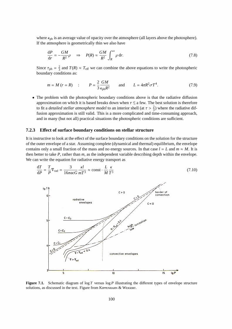
Figure 7.1. Schematic diagram of logT versus logP illustrating the different types of envelope structuresolutions, as discussed in the text. Figure from Kippenhahn & Weigert.

100

5 10 15

4

5

6

7

log P (dyn/cm2)

log

T (

K)

log P (dyn/cm2)

log

T (

K)

log P (dyn/cm2)

log

T (

K)

log P (dyn/cm2)

log

T (

K)

log P (dyn/cm2)

log

T (

K)

log P (dyn/cm2)

log

T (

K)

log P (dyn/cm2)

log

T (

K)

ZAMS models, Z = 0.02

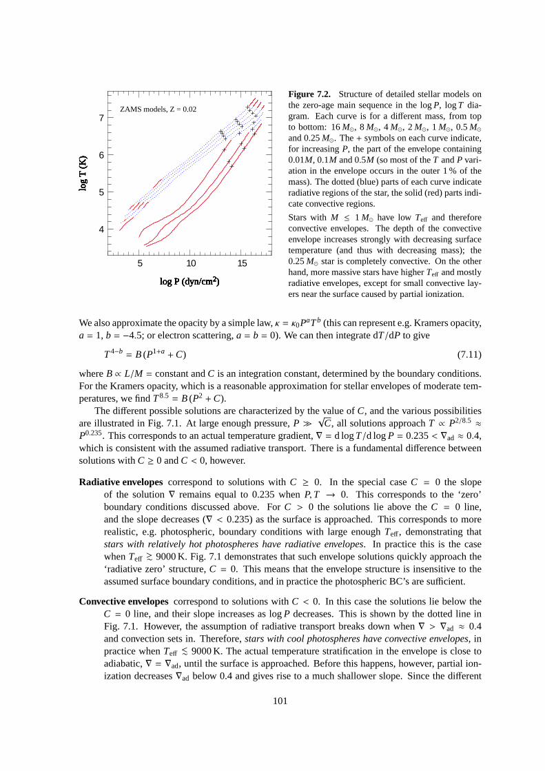
Figure 7.2. Structure of detailed stellar models onthe zero-age main sequence in the logP, logT dia-gram. Each curve is for a different mass, from topto bottom: 16M⊙, 8M⊙, 4M⊙, 2M⊙, 1M⊙, 0.5M⊙and 0.25M⊙. The+ symbols on each curve indicate,for increasingP, the part of the envelope containing0.01M, 0.1M and 0.5M (so most of theT andP vari-ation in the envelope occurs in the outer 1 % of themass). The dotted (blue) parts of each curve indicateradiative regions of the star, the solid (red) parts indi-cate convective regions.

Stars withM ≤ 1 M⊙ have lowTeff and thereforeconvective envelopes. The depth of the convectiveenvelope increases strongly with decreasing surfacetemperature (and thus with decreasing mass); the0.25M⊙ star is completely convective. On the otherhand, more massive stars have higherTeff and mostlyradiative envelopes, except for small convective lay-ers near the surface caused by partial ionization.

We also approximate the opacity by a simple law,κ = κ0PaTb (this can represent e.g. Kramers opacity,a = 1, b = −4.5; or electron scattering,a = b = 0). We can then integrate dT/dP to give

T4−b = B (P1+a +C) (7.11)

whereB ∝ L/M = constant andC is an integration constant, determined by the boundary conditions.For the Kramers opacity, which is a reasonable approximation for stellar envelopes of moderate tem-peratures, we findT8.5 = B (P2 +C).

The different possible solutions are characterized by the value ofC, and the various possibilitiesare illustrated in Fig. 7.1. At large enough pressure,P ≫

√C, all solutions approachT ∝ P2/8.5 ≈

P0.235. This corresponds to an actual temperature gradient,∇ = d logT/d logP = 0.235< ∇ad ≈ 0.4,which is consistent with the assumed radiative transport. There is a fundamental difference betweensolutions withC ≥ 0 andC < 0, however.

Radiative envelopescorrespond to solutions withC ≥ 0. In the special caseC = 0 the slopeof the solution∇ remains equal to 0.235 whenP,T → 0. This corresponds to the ‘zero’boundary conditions discussed above. ForC > 0 the solutions lie above theC = 0 line,and the slope decreases (∇ < 0.235) as the surface is approached. This corresponds to morerealistic, e.g. photospheric, boundary conditions with large enoughTeff, demonstrating thatstars with relatively hot photospheres have radiative envelopes. In practice this is the casewhenTeff ∼> 9000 K. Fig. 7.1 demonstrates that such envelope solutions quickly approach the‘radiative zero’ structure,C = 0. This means that the envelope structure is insensitive to theassumed surface boundary conditions, and in practice the photosphericBC’s are sufficient.

Convective envelopescorrespond to solutions withC < 0. In this case the solutions lie below theC = 0 line, and their slope increases as logP decreases. This is shown by the dotted line inFig. 7.1. However, the assumption of radiative transport breaks down when∇ > ∇ad ≈ 0.4and convection sets in. Therefore,stars with cool photospheres have convective envelopes, inpractice whenTeff ∼< 9000 K. The actual temperature stratification in the envelope is close toadiabatic,∇ = ∇ad, until the surface is approached. Before this happens, however, partial ion-ization decreases∇ad below 0.4 and gives rise to a much shallower slope. Since the different

101

solution lie close together near the surface, but further apart in the interior, the structure of aconvective envelopeis sensitive to the surface boundary conditions. This means that the struc-ture also depends on the uncertain details of near-surface convection (see Sec. 5.5). A smallchange or uncertainty inTeff can have a large effect on the depth of the convective envelope!For small enoughTeff the whole star can become convective (leading to the Hayashi line in theH-R diagram, see Sect. 9.1.1).

The approximate description given here is borne out by detailed stellar structure calculations, asdemonstrated in Fig. 7.2. Also note that if we assume electron scattering insteadof Kramers opacity,the description remains qualitatively the same (the radiative zero solution then has∇ = 0.25 insteadof 0.235).

7.3 Equilibrium stellar models

For a star in both hydrostatic and thermal equilibrium, the four partial differential equations for stellarstructure (eqs. 7.1–7.4) reduce to ordinary, time-independent differential equations. We can furthersimplify the situation somewhat, by ignoring possible neutrino losses (ǫν) which are only important invery late stages of evolution, and ignoring the superadiabaticity of the temperature gradient in surfaceconvection zones. We then arrive at the following set of structure equations that determine the stellarstructure for a given composition profileXi(m):

drdm=

14πr2ρ

(7.12)

dPdm= − Gm

4πr4(7.13)

dldm= ǫnuc (7.14)

dTdm= − Gm

4πr4

TP∇ with ∇ =

∇rad =3κ

16πacGlP

mT4if ∇rad ≤ ∇ad

∇ad if ∇rad > ∇ad

(7.15)

We note that the first two equations (7.12 and 7.13) describe themechanical structureof the star, andthe last two equations (7.14 and 7.15) describe thethermal and energeticstructure. They are coupledto each other through the fact that, for a general equation of state,P is a function of bothρ andT.

Although simpler than the full set of evolution equations, this set still has no simple, analyticsolutions. The reasons are that, first of all, the equations are very non-linear: e.g.ǫnuc ∝ ρTν withν ≫ 1, andκ is a complicated function ofρ andT. Secondly, the four differential equations arecoupled and have to be solved simultaneously. Finally, the equations have boundary conditions atboth ends, and thus require iteration to obtain a solution.

It is, however, possible to make additional simplifying assumptions so that under certain cir-cumstances an analytic solution or a much simpler numerical solution is possible. We have alreadydiscussed one example of such a simplifying approach in Chapter 4, namely the case ofpolytropicmodelsin which the pressure and density are related by an equation of the form

P = K ργ.

Since in this caseP does not depend onT, the mechanical structure of a stellar model can be computedin a simple way, independent of its thermal and energetic properties, by solving eqs. (7.12) and (7.13).

102

Another approach is to consider simple scaling relations between stellar modelswith differentmasses and radii, but all having the same (or a very similar) relative density distributions. If a detailednumerical solution can be computed for one particular star, these so-calledhomology relationscan beused to find an approximate model for another star.

7.4 Homology relations

Solving the stellar structure equations almost always requires heavy numerical calculations, such asare applied in detailed stellar evolution codes. However, there is often a kindof similarity betweenthe numerical solutions for different stars. These can be approximated by simple analytical scalingrelations known ashomology relations. In past chapters we have already applied simple scalingrelations based on rough estimates of quantities appearing in the stellar structure equations. In thissection we will put these relations on a firmer mathematical footing.

The requirements for the validity of homology are very restrictive, and hardly ever apply to re-alistic stellar models. However, homology relations can offer a rough but sometimes very helpfulbasis for interpreting the detailed numerical solutions. This applies to models forstars on themainsequenceand to so-calledhomologous contraction.

Definition Compare two stellar models, with massesM1 and M2 and radiiR1 andR2. All interiorquantities in star 1 are denoted by subscript ’1’ (e.g. the mass coordinatem1), etc. Now considerso-calledhomologous mass shellswhich have the same relative mass coordinate,x ≡ m/M, i.e.

x =m1

M1=

m2

M2(7.16)

The two stellar models are said to behomologousif homologous mass shells within them arelocated at the same relative radiir/R, i.e.

r1(x)R1=

r2(x)R2

orr1(x)r2(x)

=R1

R2(7.17)

for all x.

Comparing two homologous stars, the ratio of radiir1/r2 for homologous mass shells is constant. Inother words, two homologous stars havethe same relative mass distribution, and therefore (as weshall prove shortly) the same relative density distribution.

All models have to obey the stellar structure equations, so that the transition for one homologousmodel to another has consequences for all other variables. We start byanalysing the first two structureequations.

• The first stellar structure equation (7.12) can be written for star 1 as

dr1

dx=

M1

4πr12ρ1

(7.18)

If the stars are homologous, then from eq. (7.17) we can substituter1 = r2 (R1/R2) and obtain

dr2

dx=

M2

4πr22ρ2·[

ρ2

ρ1

M1

M2

(R2

R1

)3]

. (7.19)

103

We recognize the structure equation for the radius of star 2 (i.e. eq. 7.18 with subscript ‘1’ re-placed by ‘2’), multiplied by the factor in square brackets on the right-handside. This equationmust hold generally, which is only the case if the factor in square brackets isequal to one forall values ofx, that is if

ρ2(x)ρ1(x)

=M2

M1

(R2

R1

)−3

. (7.20)

This must hold at any homologous mass shell, and therefore also at the centre of each star. Thefactor M R−3 is proportional to the average density ¯ρ, so that the density at any homologousshell scales with the central density, or with the average density:

ρ(x) ∝ ρc ∝ ρ (7.21)

Note that, therefore, any two polytropic models with the same indexn are homologous to eachother.

• We can apply a similar analysis to the second structure equation (7.13) for hydrostatic equilib-rium. For star 1 we have

dP1

dx= −GM1

2x

4πr14

(7.22)

so that after substitutingr1 = r2 (R1/R2) we obtain

dP1

dx= −GM2

2x

4πr24·[

(M1

M2

)2 (R2

R1

)4]

=dP2

dx·[

(M1

M2

)2 (R2

R1

)4]

, (7.23)

where the second equality follows because star 2 must also obey the hydrostatic equilibriumequation. Hence we have dP1/dx = C dP2/dx, with C equal to the (constant) factor in squarebrackets. Integrating we obtainP1(x) = C P2(x) + B, where the integration constantB = 0because at the surface,x→ 1, for both starsP→ 0. Thus we obtain

P2(x)P1(x)

=

(

M2

M1

)2 (

R2

R1

)−4

, (7.24)

at any homologous mass shell. Again this must include the centre, so that for all x:

P(x) ∝ Pc ∝M2

R4. (7.25)

The pressure required for hydrostatic equilibrium therefore scales withM2/R4 at any homolo-gous shell. Note that we found the same scaling of thecentralpressure withM andR from ourrough estimate in Sect. 2.2, and for polytropic models of the same indexn.

We can combine eqs. (7.20) and (7.24) to show that two homologous stars mustobey the followingrelation between pressure and density at homologous points,

P2(x)P1(x)

=

(

M2

M1

)2/3 (

ρ2(x)ρ1(x)

)4/3

, (7.26)

or

P(x) ∝ M2/3ρ(x)4/3. (7.27)

104

7.4.1 Homology for radiative stars composed of ideal gas

In order to obtain simple homology relations from the other structure equations, we must make addi-tional assumptions. We start by analysing eq. (7.15).

• First, let us assume theideal gasequation of state,

P =RµρT.

Let us further assume that in each star thecomposition is homogeneous, so thatµ is a constantfor both stars, though not necessarily the same. We can then combine eqs.(7.20) and (7.24) toobtain a relation between the temperatures at homologous mass shells,

T2(x)T1(x)

=µ2

µ1

M2

M1

(

R2

R1

)−1

or T(x) ∝ Tc ∝ µMR

(7.28)

• Second, we will assume the stars are inradiative equilibrium. We can then write eq. (7.15) as

d(T4)dx

= − 3M

16π2ac

κl

r4(7.29)

This contains two as yet unknown functions ofx on the right-hand side,κ andl. We must there-fore make additional assumptions about the opacity, which we can very roughly approximateby a power law,

κ = κ0 ρaTb. (7.30)

For a Kramers opacity law, we would havea = 1 andb = −3.5. However, for simplicity let usassume aconstant opacitythroughout each star (but likeµ, not necessarily the same for bothstars). Then a similar reasoning as was held above for the pressure, allows us to transformeq. (7.29) into an expression for the ratio of luminosities at homologous points,

(

T2(x)T1(x)

)4

=l2(x)l1(x)

M2

M1

κ2

κ1

(

R2

R1

)−4

⇒ l2(x)l1(x)

=

(

µ2

µ1

)4 (

M2

M1

)3 (

κ2

κ1

)−1

(7.31)

making use of eq. (7.28) to obtain the second expression. This relation alsoholds for the surfacelayer, i.e. for the total stellar luminosityL. Hencel(x) ∝ L and

L ∝ 1κµ4M3 (7.32)

This relation represents amass-luminosity relationfor a radiative, homogeneous star with con-stant opacity and ideal-gas pressure.

Note that we obtained a mass-luminosity relation (7.32) without making any assumption about themode of energy generation (and indeed, without even having to assume thermal equilibrium, becausewe have not yet made use of eq. 7.14). We can thus expect a mass-luminosity relation to hold notonly on the main-sequence, but for any star in radiative equilibrium. What this relation tells us is thatthe luminosity depends mainly on how efficiently energy can be transported by radiation: a higher

105

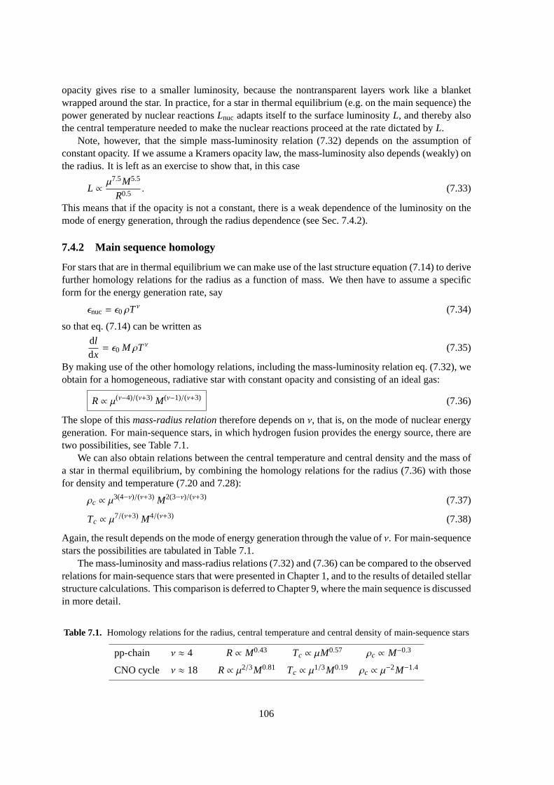
opacity gives rise to a smaller luminosity, because the nontransparent layers work like a blanketwrapped around the star. In practice, for a star in thermal equilibrium (e.g. on the main sequence) thepower generated by nuclear reactionsLnuc adapts itself to the surface luminosityL, and thereby alsothe central temperature needed to make the nuclear reactions proceed at the rate dictated byL.

Note, however, that the simple mass-luminosity relation (7.32) depends on the assumption ofconstant opacity. If we assume a Kramers opacity law, the mass-luminosity alsodepends (weakly) onthe radius. It is left as an exercise to show that, in this case

L ∝ µ7.5M5.5

R0.5. (7.33)

This means that if the opacity is not a constant, there is a weak dependence of the luminosity on themode of energy generation, through the radius dependence (see Sec.7.4.2).

7.4.2 Main sequence homology

For stars that are in thermal equilibrium we can make use of the last structureequation (7.14) to derivefurther homology relations for the radius as a function of mass. We then have to assume a specificform for the energy generation rate, say

ǫnuc = ǫ0 ρTν (7.34)

so that eq. (7.14) can be written as

dldx= ǫ0 M ρTν (7.35)

By making use of the other homology relations, including the mass-luminosity relation eq. (7.32), weobtain for a homogeneous, radiative star with constant opacity and consisting of an ideal gas:

R∝ µ(ν−4)/(ν+3) M(ν−1)/(ν+3) (7.36)

The slope of thismass-radius relationtherefore depends onν, that is, on the mode of nuclear energygeneration. For main-sequence stars, in which hydrogen fusion provides the energy source, there aretwo possibilities, see Table 7.1.

We can also obtain relations between the central temperature and central density and the mass ofa star in thermal equilibrium, by combining the homology relations for the radius (7.36) with thosefor density and temperature (7.20 and 7.28):

ρc ∝ µ3(4−ν)/(ν+3) M2(3−ν)/(ν+3) (7.37)

Tc ∝ µ7/(ν+3) M4/(ν+3) (7.38)

Again, the result depends on the mode of energy generation through the value ofν. For main-sequencestars the possibilities are tabulated in Table 7.1.

The mass-luminosity and mass-radius relations (7.32) and (7.36) can be compared to the observedrelations for main-sequence stars that were presented in Chapter 1, andto the results of detailed stellarstructure calculations. This comparison is deferred to Chapter 9, where the main sequence is discussedin more detail.

Table 7.1. Homology relations for the radius, central temperature andcentral density of main-sequence stars

pp-chain ν ≈ 4 R∝ M0.43 Tc ∝ µM0.57 ρc ∝ M−0.3

CNO cycle ν ≈ 18 R∝ µ2/3M0.81 Tc ∝ µ1/3M0.19 ρc ∝ µ−2M−1.4

106

7.4.3 Homologous contraction

We have seen in Chapter 2 that, as a consequence of the virial theorem, a star without internal energysources must contract under the influence of its own self-gravity. Suppose that this contraction takesplace homologously. According to eq. (7.17) each mass shell inside the starthen maintains the samerelative radiusr/R. Writing r = ∂r/∂t, etc., this means that

r(m)r(m)

=RR.

Since in this case we compare homologous models with the same massM, we can replacex by themass coordinatem. For the change in density we obtain from eq. (7.20) that

ρ(m)ρ(m)

= −3RR, (7.39)

and if the contraction occursquasi-statically, i.e. slow enough to maintain HE, then the change inpressure follows from eq. (7.24),

P(m)P(m)

= −4RR=

43ρ(m)ρ(m)

. (7.40)

To obtain the change in temperature for a homologously contracting star, we have to consider theequation of state. Writing the equation of state in its general, differential form eq. (3.48) we caneliminateP/P to get

TT=

1χT

(43− χρ

)

ρ

ρ=

1χT

(3χρ − 4)RR. (7.41)

Hence the temperature increases as a result of contraction as long asχρ <43. For an ideal gas,

with χρ = 1, the temperature indeed increases upon contraction, in accordance with our (qualitative)conclusion from the virial theorem. Quantitatively,

TT=

13ρ

ρ.

However, for a degenerate electron gas withχρ = 53 eq. (7.41) shows that the temperature decreases,

in other words a degenerate gas sphere willcool upon contraction. The full consequences of thisimportant result will be explored in Chapter 8.

7.5 Stellar stability

We have so far considered stars in both hydrostatic and thermal equilibrium.But an important ques-tion that remains to be answered is whether these equilibria arestable. From the fact that stars canpreserve their properties for very long periods of time, we can guess that this is indeed the case. Butin order to answer the question of stability, and find out under what circumstances stars may becomeunstable, we must test what happens when the equilibrium situation is perturbed: will the perturba-tion be quenched (stable situation) or will it grow (unstable situation). Since there are two kinds ofequilibria, we have to consider two kinds of stability:

• dynamical stability: what happens when hydrostatic equilibrium is perturbed?

• thermal (secular) stability: what happens when the thermal equilibrium situation is perturbed?

107

7.5.1 Dynamical stability of stars

The question of dynamical stability relates to the response of a certain part of a star to a perturbationof the balance of forces that act on it: in other words, a perturbation of hydrostatic equilibrium. Wealready treated the case of dynamical stability tolocal perturbations in Sec. 5.5.1, and saw that in thiscase instability gives rise toconvection. In this section we look at the global stability of concentriclayers within a star to radial perturbations, i.e. compression or expansion.A rigorous treatment ofthis problem is very complicated, so we will only look at a very simplified example toillustrate theprinciples.

Suppose a star in hydrostatic equilibrium is compressed on a short timescale,τ ≪ τKH , so thatthe compression can be considered as adiabatic. Furthermore suppose that the compression occurshomologously, such that its radius decreases fromR to R′. Then the density at any layer in the starbecomes

ρ→ ρ′ = ρ(

R′

R

)−3

and the new pressure after compression becomesP′, given by the adiabatic relation

P′

P=

(

ρ′

ρ

)γad

=

(

R′

R

)−3γad

.

The pressure required for HE after homologous contraction is

(

P′

P

)

HE=

(

ρ′

ρ

)4/3

=

(

R′

R

)−4

Therefore, ifγad >43 thenP′ > P′HE and the excess pressure leads to re-expansion (on the dynamical

timescaleτdyn) so that HE is restored. If, however,γad <43 thenP′ < P′HE and the increase of pressure

is not sufficient to restore HE. The compression will therefore reinforce itself, andthe situation isunstable on the dynamical timescale. We have thus obtained a criterion fordynamical stability:

γad >43 (7.42)

It can be shown rigorously that a star that hasγad >43 everywhere is dynamically stable, and ifγad =

43

it is neutrally stable. However, the situation whenγad <43 in some part of the star requires further

investigation. It turns out that global dynamical instability is obtained when theintegral∫

(

γad−43

)Pρ

dm (7.43)

over the whole star is negative. Therefore ifγad <43 in a sufficiently large core, whereP/ρ is high,

the star becomes unstable. However ifγad <43 in the outer layers whereP/ρ is small, the star as a

whole need not become unstable.

Cases of dynamical instability

Stars dominated by an ideal gas or by non-relativistic degenerate electrons haveγad =53 and are

therefore dynamically stable. However, we have seen that for relativisticparticlesγad→ 43 and stars

dominated by such particles tend towards a neutrally stable state. A small disturbance of such a starcould either lead to a collapse or an explosion. This is the case ifradiation pressuredominates (athighT and lowρ), or the pressure of relativistically degenerate electrons (at very highρ).

108

A process that can lead toγad <43 is partial ionization (e.g. H↔ H+ + e−), as we have seen

in Sec. 3.5. Since this normally occurs in the very outer layers, whereP/ρ is small, it does notlead to overall dynamical instability of the star. However, partial ionization is connected to drivingoscillations in some kinds of star.

At very high temperatures two other processes can occur that have a similar effect to ionization.These arepair creation(γ + γ ↔ e+ + e−, see Sect. 3.6.2) andphoto-disintegrationof nuclei (e.g.γ + Fe↔ α). These processes, that may occur in massive stars in late stages of evolution, also leadto γad <

43 but now in the core of the star. These processes can lead to a stellar explosion or collapse

(see Chapter 13).

7.5.2 Secular stability of stars

The question of thermal orsecularstability, i.e. the stability of thermal equilibrium, is intimatelylinked to the virial theorem. In the case of an ideal gas the virial theorem (Sect. 2.3) tells us that thetotal energy of a star is

Etot = −Eint =12Egr, (7.44)

which is negative: the star is bound. The rate of change of the total energy is given by the differencebetween the rate of nuclear energy generation in the deep interior and the rate of energy loss in theform of radiation from the surface:

Etot = Lnuc− L (7.45)

In a state of thermal equilibrium,L = Lnuc andEtot remains constant. Consider now a small pertur-bation of this situation, for instanceLnuc > L because of a small temperature fluctuation. This leadsto an increase of the total energy,δEtot > 0, and since the total energy is negative, its absolute valuebecomes smaller. The virial theorem, eq. (7.44), then tells us that (1)δEgr > 0, in other words the starwill expand (δρ < 0), and (2)δEint < 0, meaning that the overall temperature will decrease (δT < 0).Since the nuclear energy generation rateǫnuc ∝ ρTν depends on positive powers ofρ and especiallyT, the total nuclear energy generation will decrease:δLnuc < 0. Eq. (7.45) shows that the perturbationto Etot will be quenched and the state of thermal equilibrium will be restored.

The secular stability of nuclear burning thus depends on thenegative heat capacityof stars com-posed of ideal gas: the property that an increase of the total energy content leads to a decrease ofthe temperature. This property provides athermostatthat keeps the temperature nearly constant andkeeps stars in a stable state of thermal equilibrium for such long time scales.

We can generalise this to the case of stars with appreciable radiation pressure. For a mixture ofideal gas and radiation we can write, with the help of eqs. (3.11) and (3.12),

Pρ=

Pgas

ρ+

Prad

ρ= 2

3ugas+13urad. (7.46)

Applying the virial theorem in its general form, eq. (2.24), this yields

2Eint,gas+ Eint,rad = −Egr (7.47)

and the total energy becomes

Etot = −Eint,gas=12(Egr + Eint,rad). (7.48)

The radiation pressure thus has the effect of reducing the effective gravitational potential energy. Ifβ = Pgas/P is constant throughout the star, then eq. (7.48) becomes

Etot =12βEgr (7.49)

109

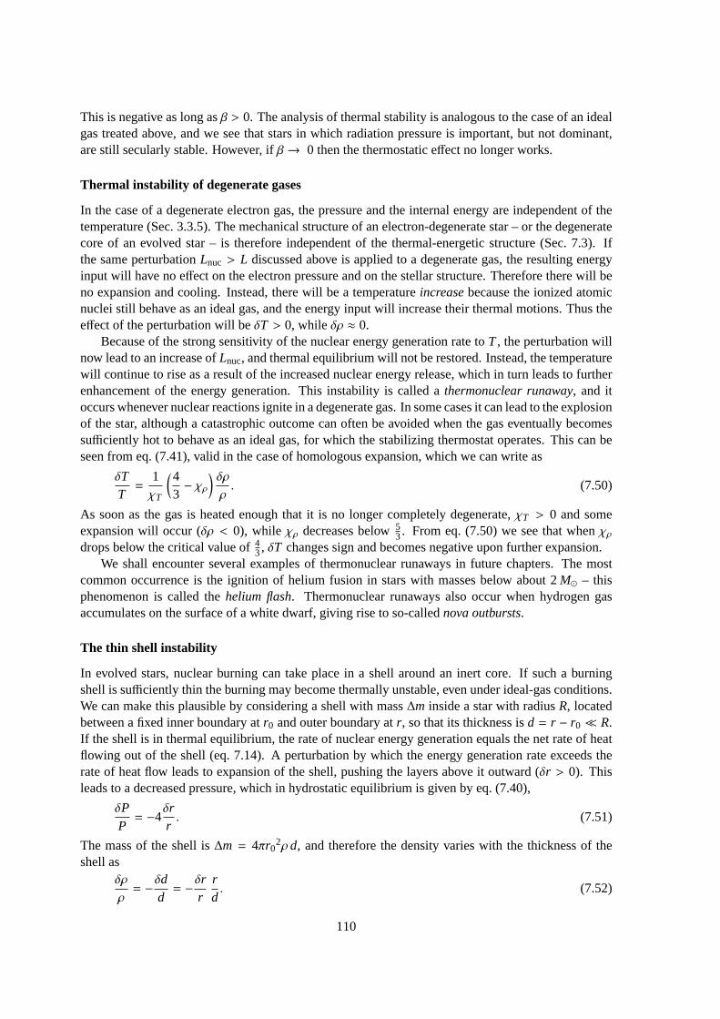
This is negative as long asβ > 0. The analysis of thermal stability is analogous to the case of an idealgas treated above, and we see that stars in which radiation pressure is important, but not dominant,are still secularly stable. However, ifβ→ 0 then the thermostatic effect no longer works.

Thermal instability of degenerate gases

In the case of a degenerate electron gas, the pressure and the internalenergy are independent of thetemperature (Sec. 3.3.5). The mechanical structure of an electron-degenerate star – or the degeneratecore of an evolved star – is therefore independent of the thermal-energetic structure (Sec. 7.3). Ifthe same perturbationLnuc > L discussed above is applied to a degenerate gas, the resulting energyinput will have no effect on the electron pressure and on the stellar structure. Therefore there will beno expansion and cooling. Instead, there will be a temperatureincreasebecause the ionized atomicnuclei still behave as an ideal gas, and the energy input will increase their thermal motions. Thus theeffect of the perturbation will beδT > 0, whileδρ ≈ 0.

Because of the strong sensitivity of the nuclear energy generation rate toT, the perturbation willnow lead to an increase ofLnuc, and thermal equilibrium will not be restored. Instead, the temperaturewill continue to rise as a result of the increased nuclear energy release,which in turn leads to furtherenhancement of the energy generation. This instability is called athermonuclear runaway, and itoccurs whenever nuclear reactions ignite in a degenerate gas. In some cases it can lead to the explosionof the star, although a catastrophic outcome can often be avoided when the gas eventually becomessufficiently hot to behave as an ideal gas, for which the stabilizing thermostat operates. This can beseen from eq. (7.41), valid in the case of homologous expansion, which we can write as

δTT=

1χT

(43− χρ

)

δρ

ρ. (7.50)

As soon as the gas is heated enough that it is no longer completely degenerate, χT > 0 and someexpansion will occur (δρ < 0), while χρ decreases below53. From eq. (7.50) we see that whenχρdrops below the critical value of43, δT changes sign and becomes negative upon further expansion.

We shall encounter several examples of thermonuclear runaways in future chapters. The mostcommon occurrence is the ignition of helium fusion in stars with masses below about 2M⊙ – thisphenomenon is called thehelium flash. Thermonuclear runaways also occur when hydrogen gasaccumulates on the surface of a white dwarf, giving rise to so-callednova outbursts.

The thin shell instability

In evolved stars, nuclear burning can take place in a shell around an inert core. If such a burningshell is sufficiently thin the burning may become thermally unstable, even under ideal-gas conditions.We can make this plausible by considering a shell with mass∆m inside a star with radiusR, locatedbetween a fixed inner boundary atr0 and outer boundary atr, so that its thickness isd = r − r0 ≪ R.If the shell is in thermal equilibrium, the rate of nuclear energy generation equals the net rate of heatflowing out of the shell (eq. 7.14). A perturbation by which the energy generation rate exceeds therate of heat flow leads to expansion of the shell, pushing the layers aboveit outward (δr > 0). Thisleads to a decreased pressure, which in hydrostatic equilibrium is given by eq. (7.40),

δPP= −4

δrr. (7.51)

The mass of the shell is∆m = 4πr02ρ d, and therefore the density varies with the thickness of the

shell asδρ

ρ= −δd

d= −δr

rrd. (7.52)

110

Eliminating δr/r from the above equations yields a relation between the changes in pressure anddensity,

δPP= 4

drδρ

ρ. (7.53)

Combining with the equation of state in its general, differential form eq. (3.48) we can eliminateδP/Pto obtain the resulting change in temperature,

δTT=

1χT

(

4dr− χρ

)

δρ

ρ. (7.54)

The shell is thermally stable as long as expansion results in a drop in temperature, i.e. when

4dr> χρ (7.55)

sinceχT > 0. Thus, for a sufficiently thin shell a thermal instability will develop. (In the case of anideal gas, the condition 7.55 givesd/r > 0.25, but this is only very approximate.) If the shell is verythin, the expansion does not lead to a sufficient decrease in pressure to yield a temperature drop, evenin the case of an ideal gas. This may lead to a runaway situation, analogous tothe case of a degenerategas. The thermal instability of thin burning shells is important during late stages of evolution of starsup to about 8M⊙, during theasymptotic giant branch.

Suggestions for further reading

The contents of this chapter are also (partly) covered by Chapter 24 of Maeder, where the question ofstability is considered in Section 3.5. A more complete coverage of the material is given in Chapters9, 10, 19, 20 and 25 of Kippenhahn.

Exercises

7.1 General understanding of the stellar evolution equations

The differential equations (7.1–7.5) describe, for a certain location in the star at mass coordinatem, thebehaviour of and relations between radius coordinater, the pressureP, the temperatureT, the luminosityl and the mass fractionsXi of the various elementsi.

(a) Which of these equations describe the mechanical structure, which describe the thermal-energeticstructure and which describe the composition?

(b) What does∇ represent? Which two cases do we distinguish?

(c) How does the set of equations simplify when we assume hydrostatic equilibrium (HE)? If weassume HE, which equation introduces a time dependence? Which physical effect does this timedependence represent?

(d) What do the termsǫnuc andT∂s/∂t represent?

(e) How does the set of equations simplify if we also assume thermal equilibrium (TE)? Which equa-tion introduces a time dependence in TE?

(f) Equation (7.5) describes the changes in the composition. In principle we need one equation forevery possible isotope. In most stellar evolution codes, the nuclear network is simplified. Thisreduces the number of differential equations and therefore increases speed of stellar evolutioncodes. TheSTARS code behindWindow to the Starsonly takes into account seven isotopes. Whichdo you think are most important?

111

7.2 Dynamical Stability

(a) Show that for a star in hydrostatic equilibrium (dP/dm = −Gm/(4πr4)) the pressure scales withdensity asP ∝ ρ4/3.

(b) If γad < 4/3 a star becomes dynamically unstable. Explain why.

(c) In what type of starsγad ≈ 4/3?

(d) What is the effect of partial ionization (for example H⇆ H+ + e−) onγad? So what is the effect ofionization on the stability of a star?

(e) Pair creationandphoto-disintegrationof Fe have a similar effect onγad. In what type of stars (andin what phase of their evolution) do these processes play a role?

7.3 Mass radius relation for degenerate stars

(a) Derive how the radius scales with mass for stars composedof a non-relativistic completely de-generateelectron gas. Assume that the central densityρc = aρ and that the central pressurePc = bGM2/R4, whereρ is the mean density, anda andb depend only on the density distributioninside the star.

(b) Do the same for anextremely relativistic degenerateelectron gas.

(c) The electrons in a not too massive white dwarf behave likea completely degenerate non-relativisticgas. Many of these white dwarfs are found in binary systems. Describe qualitatively what happensif the white dwarf accretes material from the companion star.

7.4 Main-sequence homology relations

We speak of twohomologous starswhen they have the same density distribution. To some extentmainsequence stars can be considered as stars with a similar density distribution.

(a) You already derived some scaling relations for main sequence stars from observations in the firstset of exercises: the mass-luminosity relation and the mass-radius relation. Over which mass rangewere these simple relations valid?

(b) During the practicum you plotted the density distribution of main sequence stars of differentmasses. For which mass ranges did you find that that the stars had approximately the same densitydistribution.

(c) Compare theL-M relation derived form observational data with theL-M relation derived fromhomology, eq. (7.32). What could cause the difference? (Which assumptions may not be valid?)

(d) Show that, if we replace the assumption of a constant opacity with a Kramers opacity law, themass-luminosity-radius relation becomes eq. (7.33),

L ∝ µ7.5M5.5

R0.5.

(e) Substitute a suitable mass-radius relation and comparethe result of (d) with the observational datain Fig. 1.3. For which stars is the Kramers-basedL-M relation the best approximation? Can youexplain why? What happens at lower and higher masses, respectively?

7.5 Central behaviour of the stellar structure equations

(a) Rewrite the four structure equations in terms of d/dr.

(b) Find how the following quantities behave in the neighbourhood of the stellar center:- the massm(r),- the luminosityl(r),- the pressureP(r),- the temperatureT(r).

112

Chapter 8

Schematic stellar evolution –consequences of the virial theorem

8.1 Evolution of the stellar centre

We will consider the schematic evolution of a star, as seen from its centre. The centre is the pointwith the highest pressure and density, and (usually) the highest temperature, where nuclear burningproceeds fastest. Therefore, the centre is the most evolved part of thestar, and it sets the pace ofevolution, with the outer layers lagging behind.

The stellar centre is characterized by the central densityρc, pressurePc and temperatureTc andthe composition (usually expressed in terms ofµ and/or µe). These quantities are related by theequation of state (EOS). We can thus represent the evolution of a star by an evolutionary track in the(Pc, ρc) diagram or the (Tc, ρc) diagram.

8.1.1 Hydrostatic equilibrium and the Pc-ρc relation

Consider a star in hydrostatic equilibrium (HE), for which we can estimate howthe central pres-sure scales with mass and radius from the homology relations (Sec. 7.4). For a star that expands orcontracts homologously, we can apply eq. (7.26) to the central pressureand central density to yield

Pc = C · GM2/3ρc4/3 (8.1)

whereC is a constant. This is a fundamental relation for stars in HE:in a star of mass M that expandsor contracts homologously, the central pressure varies as central density to the power43. The valueof the constantC depends on the density distribution in the star. Note that we found the same relationfor polytropic stellar models in Chapter 4, eq. (4.18), whereC = Cn depends on the polytopic index.However, the dependence onn, and hence on the density distibution, is only very weak. For polytropicmodels with indexn = 1.5 – 3, a range that encompasses most actual stars,C varies between 0.48 and0.36. Hence relation (8.1) is reasonably accurate, even if the contractionis not exactly homologous.In other words: for a star of a certain mass, the central pressure is almost uniquely determined by thecentral density.

Note that we have obtained this relation without considering the EOS. Therefore (8.1) defines auniversal relation for stars in HEthat is independent of the equation of state. It expresses the fact thata star that contracts quasi-statically must achieve a higher internal pressure to remain in hydrostaticequilibrium. Eq. (8.1) therefore defines anevolution trackof a slowly contracting (or expanding) starin thePc-ρc plane.

113

8.1.2 The equation of state and evolution in thePc-ρc plane

By considering the EOS we can also derive the evolution of the central temperature. This is obviouslycrucial for the evolutionary fate of a star because e.g. nuclear burningrequiresTc to reach certain(high) values. We start by considering lines of constantT, isotherms, in the (P, ρ) plane.

We have encountered various regimes for the EOS in Chapter 3:

• Radiation dominated:P = 13aT4. Hence an isotherm in this region is also a line of constantP.

• (Classical) ideal gas:P =RµρT. Hence an isotherm hasP ∝ ρ.

• Non-relativistic electron degeneracy:P = KNR(ρ/µe)5/3 (eq. 3.35). This is independent of tem-perature. More accurately: the complete degeneracy implied by this relation isonly achievedwhenT → 0, so this is in fact the isotherm forT = 0 (and not too high densities).

• Extremely relativistic electron degeneracy:P = KER(ρ/µe)4/3 (eq. 3.37). This is the isothermfor T = 0 and very highρ.

Figure 8.1 shows various isotherms schematically in the logρ – logP plane. Where radiationpressure dominates (lowρ) the isotherms are horizontal and where ideal-gas pressure dominates theyhave a slope= 1. The isotherm forT = 0, corresponding to complete electron degeneracy, has slopeof 5

3 at relatively low density and a shallower slope of43 at high density. The region to the right and

below theT = 0 line is forbidden by the Pauli exclusion principle, since electrons are fermions.The dashed lines are schematic evolution tracks for stars of different massesM1 andM2. Accord-

ing to eq. (8.1) they have a slope of43 and the track for a larger mass lies at a higher pressure than that

for a smaller mass.Several important conclusions can be drawn from this diagram:

• As long as the gas is ideal, contraction (increasingρc) leads to a higherTc, because the slopeof the evolution track is steeper than that of ideal-gas isotherms: the evolutiontrack crossesisotherms of higher and higher temperature.

Figure 8.1. Schematic evolution in the logρ– logP plane. Solid lines are isotherms in the equation of state;the dashed lines indicate two evolution tracks of different mass, which have a slope of4

3. See the text for anexplanation.

114

Note that this is consistent with what we have already concluded from the virial theorem for anideal gas:Ein = −1

2Egr. Contraction (decreasingEgr, i.e. increasing−Egr) leads to increasinginternal (thermal) energy of the gas, i.e. to heating of the stellar gas!

• Tracks for masses lower than some critical valueMcrit, e.g. the track labeledM1, eventuallyrun into the line for complete electron degeneracy because this has a steeper slope. Hence forstars withM < Mcrit there exist a maximum achievable central density and pressure,ρc,max andPc,max, which define the endpoint of their evolution. This endpoint is a completely degeneratestate, i.e. a white dwarf, where the pressure needed to balance gravity comes from electronsfilling the lowest possible quantum states.

Because complete degeneracy corresponds toT = 0, it follows that the evolution track mustintersect each isotherm twice. In other words, stars withM < Mcrit also reach a maximumtemperatureTc,max, at the point where degeneracy starts to dominate the pressure, after whichfurther contraction leads to decreasingTc. ρc,max, Pc,max andTc,max all depend onM and in-crease with mass.

• Tracks for masses larger thanMcrit, e.g. the one labeledM2, miss the completely degenerateregion of the EOS, because at highρ this has the same slope as the evolution track. This changein slope is owing to the electrons becoming relativistic and as their velocity cannot exceedc,they exert less pressure than if there were no limit to their velocity. Hence, electron degeneracyis not sufficient to counteract gravity, and a star withM > Mcrit must keep on contracting andgetting hotter indefinitely – up to the point where the assumptions we have made break down,e.g. whenρ becomes so high that the protons inside the nuclei capture free electrons and aneutron gas is formed, which can also become degenerate.

Hence the evolution of stars withM > Mcrit is qualitatively different from that of stars withM < Mcrit. This critical mass is none other than theChandrasekhar massthat we have alreadyencountered in Chapter 4 (eq. 4.22)

MCh =5.836µe

2M⊙. (8.2)

It is the unique mass of a completely degenerate and extremely relativistic gas sphere. A star withM ≥ MCh must collapse under its own gravity, but the electrons become extremely relativistic – and,if M is equal to or not much larger thanMCh, also degenerate – in the process.

8.1.3 Evolution in theTc-ρc plane

We now consider how the stellar centre evolves in theTc, ρc diagram. First we divide theT, ρ planeinto regions where different processes dominate the EOS, see Sec. 3.3.7 and Fig. 3.4, reproduced inFig. 8.2a.

For a slowly contracting star in hydrostatic equilibrium equation (8.1) implies that,as long as thegas behaves like a classical ideal gas:

Rµ

Tc ρc = C GM2/3ρc4/3 → Tc =

C GR µM2/3ρc

1/3 (8.3)

(Compare to Sec. 7.4.3.) This defines an evolution track in the logT, logρ plane with slope13. Stars

with different mass evolve along tracks that lie parallel to each other, those with larger M lying athigher Tc and lowerρc. Tracks for larger mass therefore lie closer to the region where radiation

115

−5 0 5 10 4

6

8

10

log ρc

log

T c

radiation

ideal gas degenerate

NR ER

−5 0 5 10 4

6

8

10

log ρclo

g T c

0.1

1.0

10

100

MCh

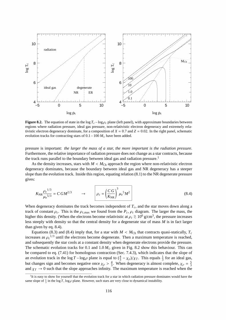
Figure 8.2. The equation of state in the logTc – logρc plane (left panel), with approximate boundaries betweenregions where radiation pressure, ideal gas pressure, non-relativistic electron degeneracy and extremely rela-tivistic electron degeneracy dominate, for a composition of X = 0.7 andZ = 0.02. In the right panel, schematicevolution tracks for contracting stars of 0.1 – 100M⊙ have been added.

pressure is important:the larger the mass of a star, the more important is the radiation pressure.Furthermore, the relative importance of radiation pressure does not change as a star contracts, becausethe track runs parallel to the boundary between ideal gas and radiation pressure.1

As the density increases, stars withM < MCh approach the region where non-relativistic electrondegeneracy dominates, because the boundary between ideal gas and NR degeneracy has a steeperslope than the evolution track. Inside this region, equating relation (8.1) to theNR degenerate pressuregives:

KNRρc

1/3

µe5/3= C GM2/3 → ρc =

(

C GKNR

)3

µe5M2 (8.4)

When degeneracy dominates the track becomes independent ofTc, and the star moves down along atrack of constantρc. This is theρc,max we found from thePc, ρc diagram. The larger the mass, thehigher this density. (When the electrons become relativistic atρc ∼> 106 g/cm3, the pressure increasesless steeply with density so that the central density for a degenerate star ofmassM is in fact largerthan given by eq. 8.4).

Equations (8.3) and (8.4) imply that, for a star withM < MCh that contracts quasi-statically,Tc

increases asρc1/3 until the electrons become degenerate. Then a maximum temperature is reached,

and subsequently the star cools at a constant density when degenerate electrons provide the pressure.The schematic evolution tracks for 0.1 and 1.0M⊙ given in Fig. 8.2 show this behaviour. This canbe compared to eq. (7.41) for homologous contraction (Sec. 7.4.3), whichindicates that the slope ofan evolution track in the logT – logρ plane is equal to (43 − χρ)/χT . This equals1

3 for an ideal gas,but changes sign and becomes negative onceχρ >

43. When degeneracy is almost complete,χρ = 5

3andχT → 0 such that the slope approaches infinity. The maximum temperature is reached when the

1It is easy to show for yourself that the evolution track for a star in which radiation pressure dominates would have thesame slope of13 in the logT, logρ plane. However, such stars are very close to dynamical instability.

116

ideal gas pressure and degenerate electron pressure are about equal, each contributing about half ofthe total pressure. Combining eqs. (8.3) and (8.4) then implies that the maximum central temperaturereached increases with stellar mass as (see Exercise 8.2)

Tc,max =C2G2

4RKNRµ µ

5/3e M4/3. (8.5)

For M > MCh, the tracks of contracting stars miss the degenerate region of theT-ρ plane, becauseat high density the boundary between ideal gas and degeneracy has thesame slope as an evolutiontrack. The pressure remains dominated by an ideal gas, andTc keeps increasing likeρc

1/3 to veryhigh values (> 1010 K). This behaviour is shown by the schematic tracks for 10 and 100M⊙.

8.2 Nuclear burning regions and limits to stellar masses

We found that stars withM < MCh reach a maximum temperature, the value of which increases withmass. This means that only gas spheres above a certain mass limit will reach temperatures sufficientlyhigh for nuclear burning. The nuclear energy generation rate is a sensitive function of the temperature,which can be written as

ǫnuc = ǫ0 ρλTν (8.6)

where for most nuclear reactions (those involving two nuclei)λ = 1, while ν depends mainly onthe masses and charges of the nuclei involved and usuallyν ≫ 1. For H-burning by the pp-chain,ν ≈ 4 and for the CNO-cycle which dominates at somewhat higher temperature,ν ≈ 18. For He-burning by the 3α reaction,ν ∼ 40 (andλ = 2 because three particles are involved). For C-burningand O-burning reactionsν is even larger. As discussed in Chapter 6, the consequences of this strongtemperature sensitivity are that

• each nuclear reaction takes place at a particular, nearly constant temperature, and

• nuclear burning cycles of subsequent heavier elements are well separated in temperature

As a star contracts and heats up, nuclear burning becomes important whenthe energy generated,Lnuc =

∫

ǫnucdm, becomes comparable to the energy radiated away from the surface,L. From thismoment on, the star can compensate its surface energy loss by nuclear energy generation: it comesinto thermal equilibrium. The first nuclear fuel to be ignited is hydrogen, atTc ∼ 107 K. From thehomology relation (7.38) we expect that the central temperature at which hydrogen fusion stabilizesshould depend on the mass approximately as

Tc = Tc,⊙ (M/M⊙)4/(ν+3) (8.7)

whereTc,⊙ ≈ 1.5 × 107 K, for a composition like that of the Sun (µ = µ⊙). We can estimate theminimum mass required for hydrogen burning by comparing this temperature to the maximum centraltemperature reached by a gas sphere of massM, eq. (8.5). By doing this (and takingC = 0.48 for ann = 1.5 polytrope) we find a minimum mass for hydrogen burning of 0.15M⊙.

Detailed calculations reveal that the minimum mass for the ignition of hydrogen in protostarsis about 2 times smaller than this simple estimate,Mmin = 0.08M⊙. Less massive objects becomepartially degenerate before the required temperature is reached and continue to contract and coolwithout ever burning hydrogen. Such objects are not stars accordingto our definition (Chapter 1) butare known asbrown dwarfs.

We have seen earlier that the contribution of radiation pressure increases with mass, and becomesdominant forM ∼> 100M⊙. A gas dominated by radiation pressure has an adiabatic indexγad =

43,

117

which means that hydrostatic equilibrium in such stars becomes marginally unstable (see Sec. 7.5.1).Therefore stars much more massive than 100M⊙ should be very unstable, and indeed none are knownto exist (while those withM > 50M⊙ indeed show signs of being close to instability, e.g. they losemass very readily).

Hence stars are limited to a rather narrow mass range of∼ 0.1 M⊙ to ∼ 100M⊙. The lowerlimit is set by the minimum temperature required for nuclear burning, and the upper limit by therequirement of dynamical stability.

8.2.1 Overall picture of stellar evolution and nuclear burning cycles

As a consequence of the virial theorem, a self-gravitating sphere composed of ideal gas in HE mustcontract and heat up as it radiates energy from the surface. The energy loss occurs at a rate

L = −Etot = Ein = −12Egr ≈

Egr

τKH(8.8)

This is the case for protostars that have formed out of an interstellar gas cloud. Their evolution, i.e.overall contraction, takes place on a thermal timescaleτKH . As the protostar contracts and heats upand its central temperature approaches 107 K, the nuclear energy generation rate (which is at firstnegligible) increases rapidly in the centre, until the burning rate matches the energy loss from thesurface:

L = −Enuc ≈Enuc

τnuc(8.9)

At this point, contraction stops andTc andρc remain approximately constant, at the values needed forhydrogen burning. The stellar centre occupies the same place in theTc-ρc diagram for about a nucleartimescaleτnuc. Remember that for a star of a certain mass,L is essentially determined by the opacity,i.e. by how efficiently the energy can be transported outwards.

When H is exhausted in the core – which how consists of He and has a mass typically ∼10% of thetotal massM – this helium core resumes its contraction. Meanwhile the layers around it expand. Thisconstitutes a large deviation from homology and relation (8.1) no longer applies to the whole star.However the core itself still contracts more or less homologously, while the weight of the envelopedecreases as a result of its expansion. Therefore relation (8.1) remains approximately valid for thecoreof the star, i.e. if we replaceM by the core massMc. The core continues to contract and heat upat a pace set by its own thermal timescale,

Lcore≈ Ein,core≈ −12Egr,core≈

Egr,core

τKH,core(8.10)

as long as the gas conditions remain ideal. It is now the He core mass, rather than the total mass ofthe star, that determines the further evolution.

Arguments similar to those used for deriving the minimum mass for H-burning leadto the ex-istence a minimum (core) mass for He-ignition, This is schematically depicted in Fig.8.3, whichsuggests that this minimum mass is larger than 1M⊙. However, the schematic tracks in Fig. 8.3 havebeen calculated for a fixed compositionX = 0.7, Z = 0.02, which is clearly no longer the valid sincethe core is composed of helium. You may verify that a He-rich composition increases the maximumcentral temperature reached for a certain mass (eq. 8.5). Detailed calculations put the minimum massfor He-ignition at≈ 0.3 M⊙. Stars with a core mass larger than this value ignite He in the centrewhenTc ≈ 108 K, which stops further contraction while the energy radiated away can be supplied

118

−5 0 5 10 4

6

8

10

log ρc

log

T c

H−b

He−b

C−bO−b

Si−b

0.1

1.0

10

100

Figure 8.3. The same schematic evolution tracks asin Fig. 8.2, together with the approximate regions inthe logTc – logρc plane where nuclear burning stagesoccur.

by He-burning reactions. This can go on for a length of time equal to the nuclear timescale of Heburning, which is about 0.1 times that of H burning. In stars with a He core mass< 0.3 M⊙ the corebecomes degenerate before reachingTc = 108 K, and in the absence of a surrounding envelope itwould cool to become a white dwarf composed of helium, as suggested by Fig.8.3. (In practice,however, H-burning in a shell around the core keeps the core hot andwhenMc has grown to≈ 0.5 M⊙He ignites in a degenerate flash.)

After the exhaustion of He in the core, the core again resumes its contractionon a thermaltimescale, until the next fuel can be ignited. Following a similar line of reasoningthe minimum(core) mass for C-burning, which requiresT ≈ 5 × 108 K, is ≈ 1.1 M⊙. Less massive cores aredestined to never ignite carbon but to become degenerate and cool as CO white dwarfs. The mini-mum core mass required for the next stage, Ne-burning, turns out to be≈ MCh. Stars that developcores withMc > MCh therefore also undergo all subsequent nuclear burning stages (Ne-, O- and Si-burning) because they never become degenerate and continue to contract and heat after each burningphase. Eventually they develop a core consisting of Fe, from which no further nuclear energy can besqueezed. The Fe core must collapse in a cataclysmic event (a supernova or a gamma-ray burst) andbecome a neutron star or black hole.

The alternation of gravitational contraction and nuclear burning stages is summarized in Table 8.1,together with the corresponding minimum masses and characteristic temperatures and energies. Theschematic picture presented in Fig. 8.3 of the evolution of stars of different masses in theT–ρ diagramcan be compared to Fig. 8.4, which shows the results of detailed calculations for various masses.

To summarize, we have obtained the following picture. Nuclear burning cycles can be seen as long-lived but temporary interruptions of the inexorable contraction of a star (or at least its core) underthe influence of gravity. This contraction is dictated by the virial theorem, anda result of the factthat stars are hot and lose energy by radiation. If the core mass is less than the Chandrasekhar mass,then the contraction can eventually be stopped (after one or more nuclear cycles) when electrondegeneracy supplies the pressure needed to withstand gravity. However if the core mass exceedsthe Chandrasekhar mass, then degeneracy pressure is not enough and contraction, interrupted bynuclear burning cycles, must continue at least until nuclear densities arereached.

119

Figure 8.4. Detailed evolution tracks in the logρc - logTc plane for masses between 1 and 15M⊙. Theinitial slope of each track (labelled pre-main sequence contraction) is equal to1

3 as expected from our simpleanalysis. When the H-ignition line is reached wiggles appearin the tracks, because the contraction is then nolonger strictly homologous. A stronger deviation from homologous contraction occurs at the end of H-burning,because only the core contracts while the outer layers expand. Accordingly, the tracks shift to higher densityappropriate for their smaller (core) mass. These deviations from homology occur at each nuclear burningstage. Consistent with our expectations, the most massive star (15M⊙) reaches C-ignition and keeps evolvingto higherT andρ. The core of the 7M⊙ star crosses the electron degeneracy border (indicated byǫF/kT = 10)before the C-ignition temperature is reached and becomes a C-O white dwarf. The lowest-mass tracks (1 and2 M⊙) cross the degeneracy border before He-ignition because their cores are less massive than 0.3M⊙. Basedon our simple analysis we would expect them to cool and becomeHe white dwarfs; however, their degenerateHe cores keep getting more massive and hotter due to H-shell burning. They finally do ignite helium in anunstable manner, the so-called He flash.

Suggestions for further reading

The schematic picture of stellar evolution presented above is very nicely explained in Chapter 7 ofPrialnik, which was one of the sources of inspiration for this chapter. The contents are only brieflycovered by Maeder in Sec. 3.4, and are somewhat scattered throughout Kippenhahn & Weigert, seesections 28.1, 33.1, 33.4 and 34.1.

120

Table 8.1. Characteristics of subsequent gravitational contractionand nuclear burning stages. Column (3)gives the total gravitational energy emitted per nucleon since the beginning, and column (5) the total nuclearenergy emitted per nucleon since the beginning. Column (6) gives the minimum mass required to ignite acertain burning stage (column 4). The last two columns give the fraction of energy emitted as photons andneutrinos, respectively.

phase T (106 K) total Egr/n main reactions totalEnuc/n Mmin γ (%) ν (%)

grav. 0→ 10 ∼ 1 keV/n 100nucl. 10→ 30 1H→ 4He 6.7 MeV/n 0.08M⊙ ∼95 ∼5grav. 30→ 100 ∼ 10 keV/n 100nucl. 100→ 300 4He→ 12C, 16O ≈ 7.4 MeV/n 0.3M⊙ ∼100 ∼0grav. 300→ 700 ∼ 100 keV/n ∼50 ∼50nucl. 700→ 1000 12C→ Mg, Ne ≈ 7.7 MeV/n 1.1M⊙ ∼0 ∼100grav. 1000→ 1500 ∼ 150 keV/n ∼100nucl. 1500→ 2000 16O→ S, Si ≈ 8.0 MeV/n 1.4M⊙ ∼100grav. 2000→ 5000 ∼ 400 keV/n Si→ . . .→ Fe ≈ 8.4 MeV/n ∼100

Exercises

8.1 Homologous contraction (1)

(a) Explain in your own words whathomologous contractionmeans.

(b) A real star does not evolve homologously. Can you give a specific example? [Think of core versusenvelope]

(c) Fig. 8.3 shows the central temperature versus the central density for schematic evolution tracks as-suming homologous contraction. Explain qualitatively what we can learn form this figure (nuclearburning cycles, difference between a 1M⊙ and a 10M⊙ star, ...)

(d) Fig. 8.4 shows the same diagram with evolution tracks from detailed (i.e. more realistic) models.Which aspects were already present in the schematic evolution tracks? When and where do theydiffer?

8.2 Homologous contraction (2)

In this question you will derive the equations that are plotted in Figure 8.2b.

(a) Use the homology relations forP andρ to derive eq. (8.1),

Pc = CGM2/3ρ4/3c

To see what happens qualitatively to a contracting star of given massM, the total gas pressure can beapproximated roughly by:

P ≈ Pid + Pdeg=RµρT + K

(

ρ

µe

)γ

(8.11)

whereγ varies between53 (non-relativistic) and43 (extremely relativistic).

(b) Combine this equation, for the case of NR degeneracy, with the central pressure of a contractingstar in hydrostatic equilibrium (eq. 8.1, assumingC ≈ 0.5) in order to find howTc depends onρc.

(c) Derive an expression for the maximum central temperature reached by a star of massM.

121

8.3 Application: minimum core mass for helium burning

Consider a star that consists completely of helium. Computean estimate for the minimum mass forwhich such a star can ignite helium, as follows.

• Assume that helium ignites atTc = 108 K.

• Assume that the critical mass can be determined by the condition that the ideal gas pressure andthe electron degeneracy pressure are equally important in the star at the moment of ignition.

• Use the homology relations for the pressure and the density.Assume thatPc,⊙ = 1017 g cm−1 s−2

andρc,⊙ = 60 g cm−3.

122