DOE ANALYSIS FOR THE Rz value

We take all the terms and perform the factor analysis. These are the significant factors as yielded by ANOVA.

STEP 1: ANOVA WITH ALL FACTORS

Let us see the design points which was used

The design points were taken from the RSM conducted.

Now let us see the residual plots vs variable

As we can see from earlier there is a problem with the Rz plot since it is not scattered across the mean line. However this is not a concern as we are most interested in gaining the significant factors and we will remodel it.

Let us look at the 4 residuals graph now also

As noted not the best fit for the model. However we will check the ANOVA also.

We get the information there is strong curvature. Rsq cannot be predicted because the degree of freedom are full. So let us now remodel the terms.

While remodelling due to hierarchy we have to include terms A, C and AD extra even though they are not significant to maintain the hierarchy.

STEP 2: IMPROVING MODEL BY USING TERMS P<0.1

Residuals vs Variable plot

The residuals against variable show a random order which looks ok and meets equal variance condition.

4 graphs residuals

The histogram plot look a little normal. The residual vs fitted value looks more or less random. Do not worry about residual vs order as they have been taken from the RSM data points. We will look at them more closely during the RSM analysis.

ANOVA analysis

The lack of fit shows that the model fits the data quite ok. Maybe it could be improved, however since there is curvature we will go ahead and conduct the RSM and try to figure out that square term. We also know the significant terms which will help in improving the RSM model.

But it is good to note the linear model generated by the ANOVA analysis

RSM of Rz Analysis

Step 3: RSM OF Rz FUNCTION WITH QUADRATIC FUNCTION WITH ALL TERMS

The residual 4 graphs show that the histogram is fairly normal shaped. The Residual vs fits looks random and the residual vs observations looks ok. Let us check the ANOVA analysis also.

The anova shows that the model fits in ok. Let see if we can improve the model further by removing the non significant interaction terms. We remove all pulse duration terms and check for the residuals and prediction model.

[THE RESIDUALS SEEMS TO FIT WELL, IS IT NECESSARY TO FURTHER IMPROVE THIS MODEL?? ]

STEP 4: TRYING TO IMPROVE MODEL BY REMOVING TERMS WITH P>0.1

The Histogram graph is showing slight skewdness which can maybe removed through a certain transformation. Residual vs order is showing a slight trend but I think is ok. Let us also check the ANOVA now.

What we see is that the model fits in a little bit better than before R pred has slightly increased.

We see the R(prediction) has increased slightly with not much loss in Rsq adjusted. However the next step could be to transform the response function for removing skewdness in the histogram.

A log transformation looks like a possible step that can be explored. Here is the Log10 transform of the response Rz and the design table shown once again. However instead of first analysing with all variables and then reducing it subsequently to improve it, there is an option called backward elimination in MINITAB which does the same function avoiding the iterations required. Here are the results after backward elimination.

STEP 5: DIRECT LOG TRANSFORMATION OF THE RESPONSE FUNCTION AND AGAIN TRYING TO FIT QUADRATIC TERMS, BACKWARD ELIMINATION OF P>0.1 INCLUDED

The 4 residual graph after backward elimination

Let us look at the ANOVA table

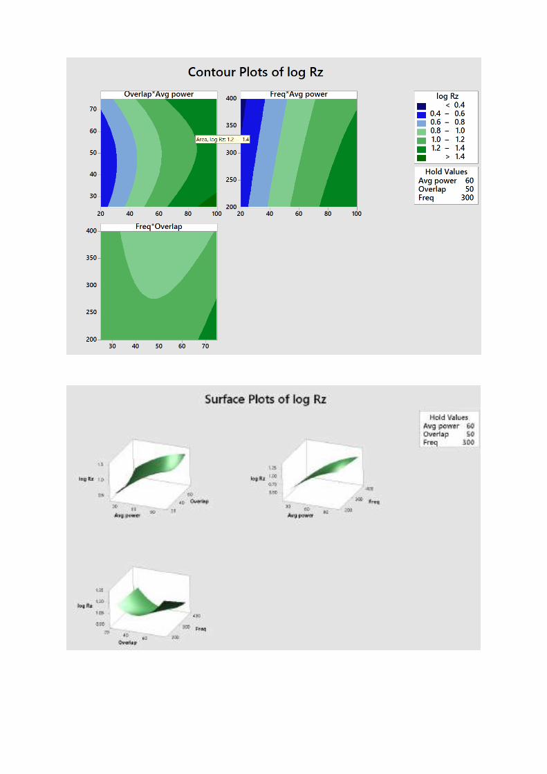
The lack of fit P value has substantially increased showing that this model fits much better than the previous models done in RSM. So I think the model is ready to use.

The regression equation is clearly shown. The outlier has been left as it is. It has been already remeasured thrice.

Now we can utilize this function for Response optimizer and confirming the runs.