Step-Up Multiple Testing of Parameters with Unequally Correlated EstimatesAuthor(s): Charles W. Dunnett and Ajit C. TamhaneSource: Biometrics, Vol. 51, No. 1 (Mar., 1995), pp. 217-227Published by: International Biometric SocietyStable URL: http://www.jstor.org/stable/2533327Accessed: 21/10/2010 18:17

Your use of the JSTOR archive indicates your acceptance of JSTOR's Terms and Conditions of Use, available athttp://www.jstor.org/page/info/about/policies/terms.jsp. JSTOR's Terms and Conditions of Use provides, in part, that unlessyou have obtained prior permission, you may not download an entire issue of a journal or multiple copies of articles, and youmay use content in the JSTOR archive only for your personal, non-commercial use.

Please contact the publisher regarding any further use of this work. Publisher contact information may be obtained athttp://www.jstor.org/action/showPublisher?publisherCode=ibs.

Each copy of any part of a JSTOR transmission must contain the same copyright notice that appears on the screen or printedpage of such transmission.

JSTOR is a not-for-profit service that helps scholars, researchers, and students discover, use, and build upon a wide range ofcontent in a trusted digital archive. We use information technology and tools to increase productivity and facilitate new formsof scholarship. For more information about JSTOR, please contact support@jstor.org.

International Biometric Society is collaborating with JSTOR to digitize, preserve and extend access toBiometrics.

http://www.jstor.org

BIOMETRICS 51, 217-227 March 1995

Step-Up Multiple Testing of Parameters With Unequally Correlated Estimates

Charles W. Dunnett Department of Mathematics and Statistics and Department of Clinical Epidemiology

and Biostatistics, McMaster University, Hamilton, Ontario L8S 4K1, Canada

and Ajit C. Tamhane

Department of Statistics and Department of Industrial Engineering and Management Sciences, Northwestern University, Evanston IL 60208, U.S.A.

SUMMARY

We consider the problem of simultaneously testing k > 2 hypotheses on parameters 01, . .. ., k using test statistics t1, ... , tk such that a specified familywise error rate a is achieved. Dunnett and Tamhane (1992a) proposed a step-up multiple test procedure, in which testing starts with the hypothesis corresponding to the least significant test statistic and proceeds towards the most significant, stopping the first time a significant test result is obtained (and rejecting the hypotheses corresponding to that and any remaining test statistics). The parameter estimates used in the t statistics were assumed to be normally distributed with a common variance, which was a known multiple of an unknown o-2, and known correlations which were equal.

In the present article, we show how the procedure can be extended to include unequally correlated parameter estimates. Unequal correlations occur, for example, in experiments involving comparisons among treatment groups with unequal sample sizes. We also compare the step-up and step-down multiple testing approaches and discuss applications to some biopharmaceutical testing problems.

1. Introduction We consider the problem of testing a set of k > 2 hypotheses H1, ..., Hk, which are to be considered jointly, rather than separately, because they are related to the same research question. We adopt the criterion that the familywise error rate (FWE), which is the probability of one or more Type I errors occurring, should be <a under any null configuration of the parameters being tested. The test statistics for testing the Hi are denoted by ti. We label the hypotheses in order of the statistical significance of the t statistics, so that H1 corresponds to the least significant test statistic and Hk the most significant. Stepwise testing of the Hi involves comparing the t statistics with a set of critical constants, c1 S * * * S Ck. The testing is carried out sequentially one hypothesis at a time and either stops or continues to the next hypothesis depending on the result observed for the particular hypothesis tested at that stage. If the testing is step-up, it starts with H1 and proceeds toward Hk, stopping the first time a rejection occurs (and rejecting all remaining hypotheses). If the testing is step-down, it starts with Hk and proceeds towards H1, stopping the first time an acceptance occurs (and accepting the remaining hypotheses).

The Newman-Keuls test is a well-known example of a step-down test. Step-down testing is better known than step-up, perhaps because it usually seems more intuitive to test the most significant hypotheses first. However, step-up testing can be advantageous in situations where the experi- menter expects to reject all or nearly all of the Hi. There are some well-known problems in biopharmaceutical testing where step-up testing should therefore be considered. Two examples are:

Key words: Adjusted p values; Biopharmaceutical testing; Familywise error rate; Multiple com- parisons with a control; Multivariate t distribution; Simulation-based quantile estimation; Simultaneous inference; Stepwise tests; Unbalanced designs.

217

218 Biometrics, March 1995

(1) Comparing k known active drugs with a placebo for the purpose of testing the sensitivity of an experiment, where it is expected that each null hypothesis of no difference between a known active drug and placebo will be rejected (see Dunnett and Tamhane (1992b)); (2) Comparing a combination drug with each of its constituents to verify that its efficacy exceeds that of any subcombination, where again it is expected, in order to justify the use of the combination drug, that each null hypothesis of no difference will be rejected (see Snapinn (1987) or Patel (1991)). Step-down testing, on the other hand, is appropriate in comparing a new drug with known standard drugs when the aim is to show, for marketing purposes, that it is superior to at least one of the standard drugs (see Dunnett and Tamhane (1992b)).

Two important step-up multiple testing procedures were proposed recently by Hommel (1988, 1989) and Hochberg (1988) (see also Hochberg and Benjamini (1990)). Both were developed by applying the closure principle to the improved Bonferroni method of Simes (1986) to obtain stepwise testing procedures for the individual hypotheses. Hochberg's method, which uses the same Bon- ferroni critical points used in the step-down method of Holm (1979), is easier to apply than Hommel's which uses a more complicated algorithm to identify the hypotheses to reject. Both methods are uniformly more powerful than Holm's method, but do not necessarily satisfy the FWE S a requirement for all cases as Holm's method does. They are known to satisfy the FWE requirement for the same cases that Simes' method does, which includes the case of independent test statistics where an analytical proof has been given as well as certain dependence cases for which simulation evidence is available.

In Dunnett and Tamhane (1992a), a normal theory based step-up procedure (denoted by SU) was developed. To test the hypotheses, it uses t statistics based upon parameter estimates assumed to be equally correlated with correlation coefficient p and with equal variances. For values of p > 0, we have found empirically that the critical values c,, for SU satisfy cm < cm, where cm denotes the Bonferroni constants used in Hochberg's procedure, over the range of values of a studied (namely, .01 < a < .20), except for m = 1 where c1 = c'j. For this reason, SU achieves higher power than Hochberg's method. It also has been shown to have higher power than Hommel's method in a numerical study (see Dunnett and Tamhane (1993)). However, the restriction to equal correlations makes it unsuitable for use in unbalanced data (unequal sample size) situations. One of the purposes of this study is to show how this restriction can be removed. We also compare SU with SD, the corresponding step-down procedure which was given in Dunnett and Tamhane (1991).

We describe the SU multiple testing procedure in Section 2.1 and define the critical constants needed to satisfy the FWE requirement. The problem of calculating the numerical values of the constants c,w for m = 1,.. , k is addressed in Section 2.2. Since the computations become progressively more difficult for m > 2, we propose two alternative methods for evaluating the cm: an approximation based on replacing unequal correlation coefficients by their arithmetic average is described in Section 2.3, and a simulation-based method is described in Section 2.4. In Section 3, the power function of SU is considered and then, in Section 4, a simulation study which shows the FWE and compares the powers of SU and SD is described. In Section 5, we discuss the computation of adjusted p values. An example is described in Section 6. In Section 7, we discuss the results obtained in the paper and also comment on the merits of step-up and step-down testing.

Throughout the article, a particular application that we have in mind and which occurs frequently in biopharmaceutical testing is the comparison of each of k treatment groups with a specified treatment group. If the sample sizes are unequal, the developments in this article are needed in order to apply the SU testing procedure described here and in Dunnett and Tamhahe (1992a, 1992b).

2. The Step-Up Test Procedure 2.1 Description For discussion purposes, consider testing a set of hypotheses against upper one-sided alternatives. (For two-sided alternatives, the changes to be made are the obvious ones.) Suppose the ith hypothesis to be tested is Hi: Hi S 0 versus the alternative Ai: Hi > 0, for 1 < i S k. Denote by 0 the parameter vector (61, . . , 6k) and by Om any parameter configuration with Hi < 0 for i = 1, ... , m and Oi > 0 for i = m + 1, ... , k. To meet the FWE requirement, we must have

P0 (accept H1, . . ., H,,) > 1 - a, for m = 1, . . ., k. (1)

Assume that least squares unbiased estimators H1, . .., 6k are available which are jointly normally distributed with var(61) = ziQo-2 and corr(61, Hj) = Pij, where ri2 and Pjare known constants depending on the design and oC2 iS an appropriate known or unknown error variance. To avoid possible dependency problems, we assume the correlation matrix 9i = {Pi> has full rank. Let S2 be an

Step- Up Multiple Testing 219

unbiased estimator of o-2 with v df such that vS2/1-2 has a X2j distribution independent of the 6i. This is the same normal theory linear model setting as in Dunnett and Tamhane (1992a) except we now allow unequal ri and pi;.

The statistics used in the SU and SD test procedures for testing the Hi are the usual t statistics and are given by ti = HilTis (where s is the observed value of S). From now on, we assume that the hypotheses have been re-labelled so that t1 < t2 < * tk. (However, the corresponding random variables, denoted by Ti, are not assumed to be ordered.) The method of calculating the critical constants for the SD procedure was given in Dunnett and Tamhane (1991). For the SU procedure, the critical constants are defined by solving the following equation recursively for Cm given c1, ... Cmi1, beginning with c1 = t', the upper a-point of Student's t with v df:

P[T(l) <c1***, T(m) <c, l=-a, for m=1, ...,k. (2)

Here T(m) < ... < T(-) denote the ordered values of T1, . .. , Tm. The latter have a central (since the left side of (2) is minimized over Om by taking Hi = 0) m-variate t distribution with v df and correlation matrix 9Jm, the correlation matrix corresponding to the m smallest t statistics. Equation (2) is the same as (3.1) in Dunnett and Tamhane (1992a), except that we have adopted a simpler notation. However, here the correlation coefficients among the Ti are no longer constrained to be equal. Since the critical constants c1, ... , c,m depend on 9m, they also depend on the observed ordering among the t statistics. For the various cases studied, it has been found empirically that the solutions to (2) always exist and satisfy the monotonicity condition c1 < C2 < ... <cm. However, this result has not been analytically established except for the case of independent test statistics: see Theorem 1 in Dalal and Mallows (1992).

Although a rigorous proof that the FWE requirement is met when the c values are determined to satisfy (2) has eluded us thus far, we can offer a heuristic explanation. When m, the number of true hypotheses, equals k, it is clear from (2) that FWE equals a when the Hi = 0, so the FWE requirement is met. Also, when m < k and the 6 values for the false hypotheses go to infinity, the T values corresponding to the true hypotheses become the smallest ones. Hence they are compared with the first m of the appropriate set of c values, so (2) ensures that FWE tends toward a. On the other hand, for small values of 6 the false hypotheses are almost true and yet their rejection is not classified as a Type I error: this makes FWE < a.

It is not obvious that the FWE is always <,a for the intermediate values of the 6i, when there are different sets of c values which come into play as the 6i increase and alter the ordering of the T values. However, computer simulations of the FWE such as the one illustrated here (see Table 3) indicate that, in fact, FWE increases monotonically and approaches a as the 6i tend to infinity. For equal correlations, there is no problem as there is only one set of values of c; in fact, in this case, it can be proved that taking the 6i -> oo for the false hypotheses is the least favorable configuration and thus FWE S a.

2.2 Solving for the Critical Constants Equation (2) must be solved recursively for cm, starting with m = 1 where the solution is c1 = t'V the a-point of univariate Student's t. For m = 2, the following equation is obtained after expansion of the left-side:

P(T(1) < c1,T(2) < c2) = P(T1 < c1,T2 < c2) + P(c1 < T1 < c2,T2 < c1) = 1 - a. (3)

The two probability expressions in the expansion are bivariate t probabilities over rectangular regions with the same correlation coefficient P12, determined by the two smallest t statistics. This equation can be solved by evaluating the two bivariate probabilities by trial and error on c2 using ci = t'. Alternatively, since there is only a single correlation coefficient involved, a solution can be obtained as described in Section 3.3 of Dunnett and Tamhane (1992a), using the computing algorithm given there.

For m = 3, we have:

P(T(1)< c, T2 < C2, T3

+ P(c1 < T1 < c2, T2 <c1, T3 < c3) + P(c1 < T1 < c2, c1 < T2 < c3, T3 < c1)

+ P(c2 < T1 < c3, T2 < c1, T3 < c2) + P(c2 < T1 < c3, c1 < T2 < c2, T3 < c1) = 1 - a. (4)

220 Biometrics, March 1995

The six probabilities on the left side are trivariate Student t integrals. In general, for any value of m ? 2, the following recursive formula defines how the region over which the probability must be evaluated can be subdivided to obtain probability expressions which can be evaluated:

[T(m) < c1, ... , T < c,,] = {T1 < Ci, [T(2) < C2, *. *, T(m, < Cmll

+ {C1 < T, < C2, [T(2) < C1, T(3) < C3, * , T(m) < c,]}

+ .. + {c,_-I < T, < c,, [T(2) < C1, ... , T(.n) < Cm-1]}. (5)

where T(2) < * < T(M) in the terms on the right-side denote the ordered values of T2, , T, with T1 separated out. This formula is similar to the one given in Lemma 3.1 of Dunnett and Tamhane (1992a) and follows using the same arguments. Formula (5) is applied recursively to the terms enclosed within square brackets. This leads to a division of the region into m! subregions which have rectangular boundaries, making it possible to evaluate the individual probabilities. Each one is a multivariate Student t probability integral with correlation matrix 9Jm, which in the case of a product correlation structure defined by pij = AiAj can be evaluated by the computer algorithm in Dunnett (1989).

We have used the above method to obtain values for the critical constants up to m = 6 for product correlation structure but found the computing times to be rather high. For example, it took up to seven times longer than for comparable constants in the equal correlation case, where the computing method in Dunnett and Tamhane (1992a) is applicable. For two-sided testing, a further complication arises due to the T values being replaced by ITI values in the equations. The effect is that intervals such as c1 < |TiJ < c2 have to be separated into components c1 < T1 < c2 and -c2 < Ti < -c1 to evaluate the probability integrals, increasing the number of terms and hence computing time still more. Thus, we recommend instead two alternative approaches for determining cm for m ? 3, which are valid when the pij are unequal and not necessarily of product structure.

The exact values shown in Table 1 were computed using the recursive formula in (5). They show that the approximate values obtained by the average-p method to be described in the next section are slightly on the conservative side. This phenomenon is similar to that found in approximating multivariate t percentage points: see Hochberg and Tamhane (1987, p. 146), Dunnett (1985), and Iyengar (1988).

2.3 Approximating the Constants c3, . C..,

The first approach is to obtain an approximate solution for Cm (m ? 3) by replacing the unequal correlation coefficients by their arithmetic averages. Thus, to determine c3 we replace P12, P13 and P23 by p3 = (P12 + P13 + P23)/3. Then we have a common p and the method described in Section 3.3 of Dunnett and Tamhane (1992a) can be used to calculate a solution which is an approximation to c3. Similarly, to determine C4, or in general c,*, we replace the ('") correlation coefficients by their arithmetic average Pm and using the previously calculated values of c1, . c. , cm1 we can calculate an approximation to cm.

2.4 Simulation-Based Estimates of c3, **.Ck

The second approach is to estimate c3, ... 1 Ck by simulation, which is feasible provided that k is not so large that sampling errors in the values of c3, . . , , Ck- 1 build up and make the estimated value of Ck too uncertain to be of practical use. We now describe a simulation procedure for estimating the value of cm, given the values of c1, ... , cm-1. (See Edwards and Berry (1987) for the principles of simulation-based estimation of a distribution percentile.) Denote by NT the total number of simu- lations to be performed and choose NT so that NO = a(NT + 1) is an integer (e.g., if a = .05 and NT = 9999, then NO = 500). Then proceed as follows:

1. Initialize a counter, NC = NO. 2. For each simulation, draw m random N(O, 1) deviates X1,.l., Xm having the desired

correlation structure corr(Xi,Xj) = pij and, if v is finite, a random X2/v variate S2. (Note: For the case of product correlation structure pij = AiAj, draw m + 1 independent N(O, 1) deviates Zo, Z * **Zm and setXi = 1 - A2Zi + A1ZO.)

3. Define Ti - X,/S if v is finite or Ti = Xi if v = oo and order the T values to obtain T(1) < * **

4. Check whether T(i) < c1, ... ., T(,n_1) < Cpz_l. If so, store the value of T(,n) and return to Step 2. Otherwise, decrease NC by 1 and return to Step 2.

Step- Up Multiple Testing 221

5. After completing the NT simulations, find the estimate of c,7 by counting down NC from the top of the ordered values of the stored T(m).

Remark. The estimate of cm is the (NT + 1 - NO)th order statistic of the T(,,,) Note that it is not necessary to store more than the NC highest T(-,,) values at any stage of the algorithm. By ordering the T(,,,) values in step 4 instead of step 5, the amount of storage space needed can be minimized.

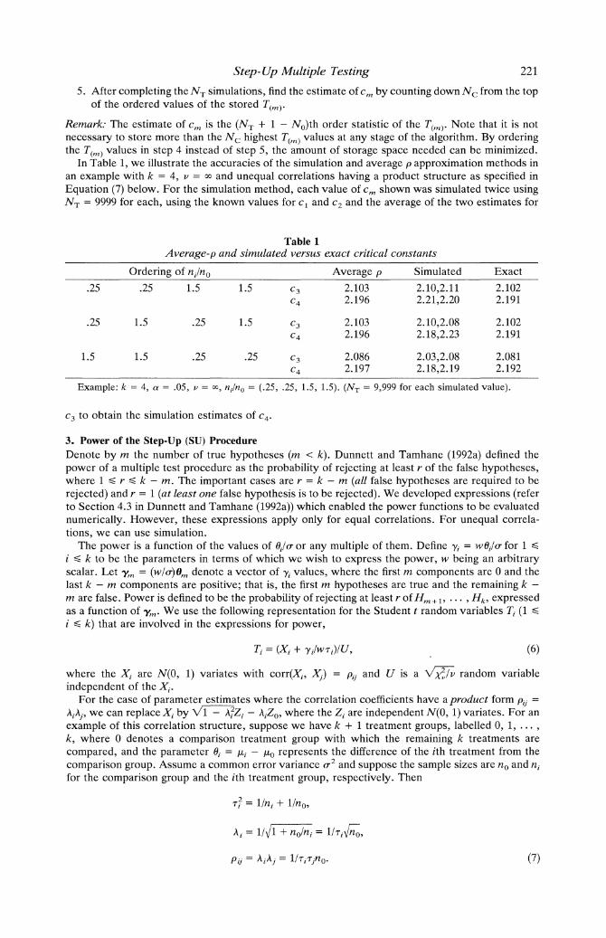
In Table 1, we illustrate the accuracies of the simulation and average p approximation methods in an example with k = 4, v = oo and unequal correlations having a product structure as specified in Equation (7) below. For the simulation method, each value of cm shown was simulated twice using NT = 9999 for each, using the known values for c1 and c2 and the average of the two estimates for

Table 1 Average-p and simulated versus exact critical constants

Ordering of ni/no Average p Simulated Exact .25 .25 1.5 1.5 C3 2.103 2.10,2.11 2.102

C4 2.196 2.21,2.20 2.191

.25 1.5 .25 1.5 C3 2.103 2.10,2.08 2.102 C4 2.196 2.18,2.23 2.191

1.5 1.5 .25 .25 C3 2.086 2.03,2.08 2.081 C4 2.197 2.18,2.19 2.192

Example: k = 4, a = .05, v = oo, ni/no = (.25, .25, 1.5, 1.5). (NT = 9,999 for each simulated value).

c3 to obtain the simulation estimates of C4.

3. Power of the Step-Up (SU) Procedure Denote by m the number of true hypotheses (m < k). Dunnett and Tamhane (1992a) defined the power of a multiple test procedure as the probability of rejecting at least r of the false hypotheses, where 1 < r < k - m. The important cases are r = k - m (all false hypotheses are required to be rejected) and r = 1 (at least one false hypothesis is to be rejected). We developed expressions (refer to Section 4.3 in Dunnett and Tamhane (1992a)) which enabled the power functions to be evaluated numerically. However, these expressions apply only for equal correlations. For unequal correla- tions, we can use simulation.

The power is a function of the values of i/ao- or any multiple of them. Define yi = w61/o- for 1 S i < k to be the parameters in terms of which we wish to express the power, w being an arbitrary scalar. Let *n = (W/o)Om denote a vector of yi values, where the first m components are 0 and the last k - m components are positive; that is, the first m hypotheses are true and the remaining k - m are false. Power is defined to be the probability of rejecting at least r of Hm ? 1, . .. , Hk, expressed as a function of 'y,,,. We use the following representation for the Student t random variables Ti (1 S i < k) that are involved in the expressions for power,

Ti = (Xi + /Yi1/W')/U. (6)

where the Xi are N(0, 1) variates with corr(Xi, Xj) = pij and U is a N/v random variable independent of the Xi.

For the case of parameter estimates where the correlation coefficients have a product form Pij= AiAj, we can replace Xi by 1- A Zi - A Zo, where the Zi are independent N(0, 1) variates. For an example of this correlation structure, suppose we have k + 1 treatment groups, labelled 0, 1, ... k, where 0 denotes a comparison treatment group with which the remaining k treatments are compared, and the parameter Hi = ,ui - ,uo represents the difference of the ith treatment from the comparison group. Assume a common error variance 0-2 and suppose the sample sizes are no and ni for the comparison group and the ith treatment group, respectively. Then

'r2 = 1/ni + 1/n_,

Ai= 1/ 1 + n0/ni = l/'ri n,

Pij = AiA1 = 1/'r1'rn0. (7)

222 Biometrics, March 1995

For this problem, we define w = Vo to standardize the power so that it does not depend on no when viewed as a function of the yi. The representation for Ti, in terms of yi, becomes

= (A1 - A7Zi- AiZo + AieY)/U. (8)

We used the above representations for Ti to obtain their values in the simulation studies in order that they would have the desired correlation structure. The power function expresses the probability that the values of T1, .. ., Tk lead to the rejection of at least r of the k - m false hypotheses, as a function of the 6Jlo- if the representation in Equation (6) is used or as a function of the yi if the representation in Equation (8) is used. In the next section, we demonstrate the simulation of both FWE and power.

4. Simulating FWE and Power Consider as an example a study with k = 4 treatments compared with a control treatment, where the sample size ratios n1/no are .25, .25, 1.5, and 1.5. These sample size ratios determine the correlation structure which is given by Equation (7). Assume o- is known, so that v = oo, which makes U _ 1 in the representation of Ti.

Two separate simulation studies were performed, one for FWE and the other for power. In the FWE study, 10,000 simulations were done for each of the six possible combinations of sample size ratios associated with the orderings of the t statistics. In each simulation, four values of m from 1 to 4 and five values of y from 0 to 20 (the latter being effectively oo) were used in order to determine the effects of altering the number of true hypotheses and the value of y for the false hypotheses. The first m sample size ratios in the initial ordering were taken to be associated with true hypotheses and the last k - m with false hypotheses. The study consisted of simulating values for the T statistics using the representation shown in Equation (8), with yi = 0 or the value displayed in the table depending on whether the associated hypothesis was to be true or false. These values were then ordered and compared with the appropriate set of critical constants. The latter were computed for each possible ordering by the average p method and the values are shown in Table 2. For each simulation and each combination of m and y, a Type I error was counted if one or more of the designated true hypotheses was rejected. Table 3 is a summary of the results, combined over all six orderings (making a total of 60,000 simulations). It shows, for this particular unequal sample size example, that over the range of values studied, the desired requirement FWE < .05 has been at least approximately achieved.

The power study was performed similarly except correct rejections were counted instead of Type

Table 2 Exact critical constants for SU and SD procedures

Constants Ordering of nJ/no cl C2 C3 C4

.25 .25 1.5 1.5 SU 1.645 1.955 2.102 2.191 SD 1.645 1.946 2.096 2.188

o25 1.5 .25 1.5 SU 1.645 1.947 2.102 2.191 SD 1.645 1.935 2.096 2.188

1.5 .25 .25 1.5 SU 1.645 1.947 2.102 2.191 SD 1.645 1.935 2.096 2.188

.25 1.5 1.5 .25 SU 1.645 1.947 2.079 2.192 SD 1.645 1.935 2.072 2.188

1.5 .25 1.5 .25 SU 1.645 1.947 2.079 2.192 SD 1.645 1.935 2.072 2.188

1.5 1.5 .25 .25 SU 1.645 1.919 2.081 2.192 SD 1.645 1.900 2.072 2.188

Example: k = 4, a = .05, v = cc, ni/n0 = (.25, .25, 1.5, 1.5).

I errors. In addition, the step-down procedure was included in order to compare results between SU and SD based on the same simulated samples. The SD critical constants were computed numerically

Step- Up Multiple Testing 223

Table 3 Simulated FWE of SUprocedure

Number Value of y1 of true Hi 0.0 1.0 2.0 4.0 20.0

1 .016 .019 .027 .039 .049 2 .028 .032 .036 .043 .049 3 .039 .041 .043 .046 .049 4 .050

Example: k = 4, ca = .05, v = o, ni/n0 = (.25, .25, 1.5, 1.5).

Table 4 Probabilities of rejecting at r false hypotheses

Number ni/no assoc'd Value of Value of false Hi with false Hi Yi of r SU SD

1 1.5 4.0 1 .818 .821 6.0 1 .991 .991

1 .25 4.0 1 .346 .349 6.0 1 .695 .697

2 .25, 1.5 4.0 1 .850 .851 2 .348 .349

6.0 1 .995 .995 2 .713 .715

3 .25, 1.5, 1.5 4.0 1 .867 .868 2 .535 .532 3 .220 .215

6.0 2 .900 .898 3 .620 .619

4 all 4.0 2 .835 .825 3 .599 .578 4 .337 .317

6.0 2 .995 .995 3 .932 .923 4 .740 .729

Example: k = 4, ca = .05, v = oco, ni/no = (.25, .25, 1.5, 1.5).

as described in Dunnett and Tamhane (1991) and the values are shown in Table 2 alongside the values for SU. Table 4 shows the power results obtained, but here the different initial sample size orderings were not pooled as they were for FWE, because the ordering determines which samples are associated with the y values and this has an influence on the power. Each power estimate shown is based upon 10,000 simulations.

The first thing to note about the results in Table 4 is that the actual power differences between the SU and SD methods are quite small. In fact, the degree of agreement between the two methods, defined as the percentage of samples where both methods detected the same numbers of false hypotheses, ranged from 97 to 99.9% for the simulations shown in the table.

It should also be pointed out that, since SU and SD were applied to the same samples, the number of simulations used in the study was sufficient to detect small differences (i.e., .002) in power. Thus, the results in Table 4 indicate that some of the differences in power, though small, are nevertheless real. They tend to favor SD when only one hypothesis is false and SU when all or most hypotheses are false. These results are qualitatively similar to the numerical results obtained for the equal-correlation case by Dunnett and Tamhane (1992a). However, although these results are suggestive, they must be qualified by emphasizing that we only have the simulation evidence displayed in Table 3 rather than an analytical proof.

5. Adjusted p Values for the Step-Up Procedure In most testing applications, it is more informative to determine p values for each hypothesis rather than merely noting whether a specific level xe has been reached. Following Westfall and Young

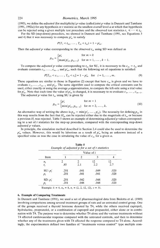
224 Biometrics, March 1995

(1993), we define the adjusted (for multiplicity)p value (called joint p value in Dunnett and Tamhane (1991, 1992a)) for any hypothesis or t statistic as the smallest overall level a at which that hypothesis can be rejected using a given multiple test procedure and the observed test statistics t1 < * * tk.

For the SD (step-down) procedure, we showed in Dunnett and Tamhane (1991, see Equations 3 and 4) that it was necessary to compute p, to satisfy

P(T1 < tin, ** Tzn < tm) =1Pm,.

Then the adjusted p value corresponding to the observed t,n using SD was defined as

Ipk for m = k

Pm lmax(p2 ,pmp + l) for m = 1, ,k - 1.

To compute the adjusted p value corresponding to tm for SU, it is necessary to fix cM = tin and evaluate constants c1, ..., cn_1 andp, , such that the following set of equations is satisfied:

P[T(1) < c . *, Tv) < ci] = 1 - P,' for i = 1, ..., m. (9)

These equations are similar to those in Equation (2) except that here cm is given and we have to evaluate c1, ..., cMl and p,2. The same algorithm used to compute the critical constants can be used, either exactly or using the average p approximation, to compute the left-side using a trial value forp, . Note that each time the value of pm is changed, it is necessary to re-evaluate c1, .l. , cM_.

The adjusted p value for tin using SU is given by

fpi form = 1

P min(p,7,p,2p1) for m = 2, .., k. (10)

An alternative way of writing the above is pm = min(p', . p.. , p). The necessity for defining p,n in this way results from the fact that Hmn can be rejected either due to the magnitude of tin or because a previous Hi was rejected. Table 5 shows an example of determining adjusted p values correspond- ing to a set of t statistics for the step-up procedure, compared with the corresponding step-down adjusted p values.

In principle, the simulation method described in Section 2.4 could also be used to determine the pm values. However, this would be laborious as a result of pn being an unknown instead of a specified value as was the case in simulating the value of c,M for a given a.

Table 5 Example of adjusted p for a set of t statistics

Value of i Item 1 2 3 4

ni 2 2 12 12 tj .85 2.1 2.2 2.7

SU: p' .201 .041 .049 .020 Pi .201 .041 .041 .020

SD: p' .201 .042 .048 .020 Pi .201 .048 .048 .020

Example: k = 4, no = 8, ni = (2, 2, 12, 12), v = 31.

6. Example of Comparing Treatments In Dunnett and Tamhane (1991), we used a set of pharmacological data from Bedotta et al. (1989) involving comparisons among several treatment groups of rats and an untreated control group. One of the groups received a thyroid hormone denoted by T4, while the others received captopril, hydralazine, propranolol, or a combination of captopril and propanolol, either alone or in combi- nation with T4. The purpose was to determine whether T4 alone and the various treatments without T4 affected cardiovascular response compared with the untreated controls, and then to determine whether any of the treatments given with T4 affected the response compared to T4 alone. Accord- ingly, the experimenters defined two families of "treatments versus control" type multiple com-

Step- Up Multiple Testing 225

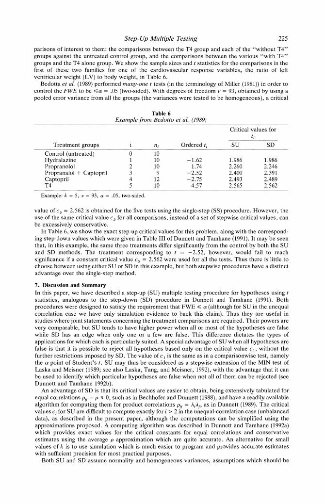
parisons of interest to them: the comparisons between the T4 group and each of the "without T4" groups against the untreated control group, and the comparisons between the various "with T4" groups and the T4 alone group. We show the sample sizes and t statistics for the comparisons in the first of these two families for one of the cardiovascular response variables, the ratio of left ventricular weight (LV) to body weight, in Table 6.

Bedotta et al. (1989) performed many-one t tests (in the terminology of Miller (1981)) in order to control the FWE to be <a = .05 (two-sided). With degrees of freedom v = 93, obtained by using a pooled error variance from all the groups (the variances were tested to be homogeneous), a critical

Table 6 Example from Bedotto et al. (1989)

Critical values for t.

Treatment groups i ni Ordered ti SU SD Control (untreated) 0 10 Hydralazine 1 10 -1.62 1.986 1.986 Propranolol 2 10 1.74 2.260 2.246 Propranalol + Captopril 3 9 -2.52 2.400 2.391 Captopril 4 12 -2.75 2.493 2.489 T4 5 10 4.57 2.565 2.562

Example: k = 5, v = 93, ca = .05, two-sided.

value of c5 = 2.562 is obtained for the five tests using the single-step (SS) procedure. However, the use of the same critical value c5 for all comparisons, instead of a set of stepwise critical values, can be excessively conservative.

In Table 6, we show the exact step-up critical values for this problem, along with the correspond- ing step-down values which were given in Table III of Dunnett and Tamhane (1991). It may be seen that, in this example, the same three treatments differ significantly from the control by both the SU and SD methods. The treatment corresponding to t = -2.52, however, would fail to reach significance if a constant critical value c5 = 2.562 were used for all the tests. Thus there is little to choose between using either SU or SD in this example, but both stepwise procedures have a distinct advantage over the single-step method.

7. Discussion and Summary In this paper, we have described a step-up (SU) multiple testing procedure for hypotheses using t statistics, analogous to the step-down (SD) procedure in Dunnett and Tamhane (1991). Both procedures were designed to satisfy the requirement that FWE < a (although for SU in the unequal correlation case we have only simulation evidence to back this claim). Thus they are useful in studies where joint statements concerning the treatment comparisons are required. Their powers are very comparable, but SU tends to have higher power when all or most of the hypotheses are false while SD has an edge when only one or a few are false. This difference dictates the types of applications for which each is particularly suited. A special advantage of SU when all hypotheses are false is that it is possible to reject all hypotheses based only on the critical value c1, without the further restrictions imposed by SD. The value of c1 is the same as in a comparisonwise test, namely the a point of Student's t. SU may thus be considered as a stepwise extension of the MIN test of Laska and Meisner (1989; see also Laska, Tang, and Meisner, 1992), with the advantage that it can be used to identify which particular hypotheses are false when not all of them can be rejected (see Dunnett and Tamhane 1992b).

An advantage of SD is that its critical values are easier to obtain, being extensively tabulated for equal correlations pij = p B 0, such as in Bechhofer and Dunnett (1988), and have a readily available algorithm for computing them for product correlations Pij = AiAj, as in Dunnett (1989). The critical values ci for SU are difficult to compute exactly for i > 2 in the unequal-correlation case (unbalanced data), as described in the present paper, although the computations can be simplified using the approximations proposed. A computing algorithm was described in Dunnett and Tamhane (1992a) which provides exact values for the critical constants for equal correlations and conservative estimates using the average p approximation which are quite accurate. An alternative for small values of k is to use simulation which is much easier to program and provides accurate estimates with sufficient precision for most practical purposes.

Both SU and SD assume normality and homogeneous variances, assumptions which should be

226 Biometrics, March 1995

verified in any application for which they are being considered. The normality assumption is the less important of the two, since the central limit theorem often makes this assumption tenable even for non-normal data. Variance heterogeneity, on the other hand, is a crucial assumption which can alter the properties of the procedures if it is present. The same strategies for dealing with this that were outlined for the SD procedure in Dunnett and Tamhane (1991) can also be used with the SU procedure.

ACKNOWLEDGEMENTS

We thank Dr. Helmut Finner and Dr. Tony Hayter for drawing our attention to the paper by Dalal and Mallows (1992) and its bearing on our work. We also thank the editors and referees for their valuable suggestions. The work of the first author was supported by a research grant from the Natural Sciences and Engineering Research Council of Canada.

RESUME

Pour r6aliser k tests d'hypotheses simultan6s (k B 2) concernant des parametres 06, ...O k, on utilise des statistiques tl, ... , tk qui permettent de controler un risque a global de rejeter a tort une ou plusieurs hypotheses nulles. Dans ce cadre, Dunnett et Tamhane (1992, Journal of the American Statistical Association 87, 162-170) avaient propose une procedure de tests multiples dite "mon- tante", oui l'on considere successivement les hypotheses nulles, dans l'ordre de significativit6 croissante des tests qui leur correspondent; on s'arrete des qu'un resultat significatif est obtenu (on rejette alors l'hypothese nulle correspondante et toutes les hypoth&ses nulles qui restaient a tester). Cet article supposait que les estimateurs des param&tres, utilis6s dans le calcul des statistiques t, 6taient normaux, de meme variance (6gale a un multiple connu d'un o 2 inconnu) et equicorr6l6s (p connu). Dans le pr6sent article, nous g6n6ralisons cette proc6dure a des cas oui les estimateurs ne sont pas 6quicorr6les (ces corr6lations in6gales se rencontrent notamment dans les essais oui les comparaisons multiples concernent des groupes de tailles diff6rentes). Par ailleurs, nous comparons les m6rites de la proc6dure "montante" a ceux de la procedure dite "descendante", et en discutons les applications a des problemes rencontr6s couramment dans l'industrie pharmaceutique.

REFERENCES

Bechhofer, R. E. and Dunnett, C. W. (1988). Tables of percentage points of multivariate t distri- butions. In Selected Tables in Mathematical Statistics, Vol. 11. Providence, Rhode Island: American Mathematical Society, pp. 1-371.

Bedotta, J. E., Gay, R. G., Graham, S. D., Morkin, E., and Goldman, S. (1989). Cardiac hyper- trophy induced by thyroid hormone is independent of loading conditions and beta adrenoceptor. Journal of Pharmacology and Experimental Therapeutics 248, 632-636.

Dalal, S. R. and Mallows, C. L. (1992). Buying with exact confidence. The Annals of Applied Probability 2, 752-765.

Dunnett, C. W. (1985). Multiple comparisons between several treatments and a specified treatment. In Lecture Notes in Statistics No. 35, Linear Statistical Inference, T. Caliiiski and W. Klonecki (eds). Berlin and New York: Springer-Verlag, pp. 39-46.

Dunnett, C. W. (1989). Multivariate normal probability integrals with product correlation structure. Algorithm AS251, Applied Statistics 38, 564-579. See also Correction Note, Applied Statistics 42, 709.

Dunnett, C. W. and Tamhane, A. C. (1991). Step-down multiple tests for comparing treatments with a control in unbalanced one-way layouts. Statistics in Medicine 10, 939-947.

Dunnett, C. W. and Tamhane, A. C. (1992a). A step-up multiple test procedure. Journal of the American Statistical Association 87, 162-170.

Dunnett, C. W. and Tamhane, A. C. (1992b). Comparisons between a new drug and active and placebo controls in an efficacy clinical trial. Statistics in Medicine 11, 1057-1063.

Dunnett, C. W. and Tamhane, A. C. (1993). Power comparisons of some step-up multiple test procedures. Statistics & Probability Letters 16, 55-58.

Edwards, D. E. and Berry, J. J. (1987). The efficiency of simulation-based multiple comparisons. Biometrics 43, 913-928.

Hochberg, Y. (1988). A sharper Bonferroni procedure for multiple tests of significance. Biometrika 75, 800-802.

Hochberg, Y. and Benjamini, Y. (1990). More powerful procedures for multiple significance testing. Statistics in Medicine 9, 811-818.

Hochberg, Y. and Tamhane, A. C. (1987). Multiple Comparison Procedures. New York: John Wiley & Sons.

Step- Up Multiple Testing 227

Holm, S. (1979). A simple sequentially rejective multiple test procedure. Scandinavian Journal of Statistics 6, 65-70.

Hommel, G. (1988). A stagewise rejective multiple test procedure based on a modified Bonferroni test. Biometrika 75, 383-386.

Hommel, G. (1989). A comparison of two modified Bonferroni procedures. Biometrika 76, 624-625. Iyengar, S. (1988). Evaluation of normal probabilities of symmetric regions. SIAM Journal on

Scientific and Statistical Computing 9, 418-423. Laska, E. M. and Meisner, M. J. (1989). Testing whether an identified treatment is best. Biometrics

45, 1139-1151. Laska, E. M., Tang, D.-E., and Meisner, M. J. (1992). Testing hypotheses about an identified

treatment when there are multiple endpoints. Journal of the American Statistical Association 87, 825-831.

Miller, R. G., Jr. (1981). Simultaneous Statistical Inference, 2nd ed. New York: McGraw Hill. Patel, H. I. (1991). Comparison of treatments in a combination therapy trial. Journal of Biophar-

maceutical Statistics 1, 171-183. Simes, R. J. (1986). An improved Bonferroni procedure for multiple tests of significance. Biometrika

30, 507-512. Snapinn, S. M. (1987). Evaluating the efficacy of a combination therapy. Statistics in Medicine 9,

657-665. Westfall, P. H. and Young, S. S. (1993). Resampling-Based Multiple Testing. New York: John

Wiley & Sons.

Received January 1993; revised November 1993; accepted January 1994.