stephen boyd ee103 stanford university december 8, 2017 · annualized return and risk i mean return...
TRANSCRIPT
Portfolio Optimization
Stephen Boyd
EE103Stanford University
December 8, 2017
Outline
Return and risk
Portfolio investment
Portfolio optimization
Return and risk 2
Return of an asset over one period
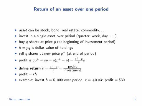
I asset can be stock, bond, real estate, commodity, . . .
I invest in a single asset over period (quarter, week, day, . . . )
I buy q shares at price p (at beginning of investment period)
I h = pq is dollar value of holdings
I sell q shares at new price p+ (at end of period)
I profit is qp+ − qp = q(p+ − p) = p+−pp h
I define return r = p+−pp =
profitinvestment
I profit = rh
I example: invest h = $1000 over period, r = +0.03: profit = $30
Return and risk 3
Short positions
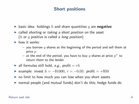
I basic idea: holdings h and share quantities q are negative
I called shorting or taking a short position on the asset(h or q positive is called a long position)
I how it works:
– you borrow q shares at the beginning of the period and sell them atprice p
– at the end of the period, you have to buy q shares at price p+ toreturn them to the lender
I all formulas still hold, e.g., profit = rh
I example: invest h = −$1000, r = −0.05: profit = +$50
I no limit to how much you can lose when you short assets
I normal people (and mutual funds) don’t do this; hedge funds do
Return and risk 4

Examples
prices of BP (BP) and Coca-Cola (KO) for last 10 years
0 500 1000 1500 2000 25000
10
20
30
40
50
60
70
Days
Price
s
KO
BP
Return and risk 5
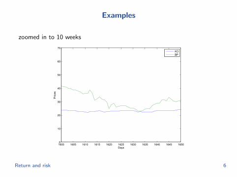
Examples
zoomed in to 10 weeks
1600 1605 1610 1615 1620 1625 1630 1635 1640 1645 16500
10
20
30
40
50
60
70
Days
Price
s
KO
BP
Return and risk 6

Examples
returns over the same period
1600 1605 1610 1615 1620 1625 1630 1635 1640 1645 1650−0.2
−0.15
−0.1
−0.05
0
0.05
0.1
0.15
0.2
Days
Re
turn
s
KO
BP
Return and risk 7
Return and risk
I suppose r is time series (vector) of returns
I average return or just return is avg(r)
I risk is std(r)
I these are the per-period return and risk
Return and risk 8

Annualized return and risk
I mean return and risk are often expressed in annualized form(i.e., per year)
I if there are P trading periods per year
– annualized return = P avg(r)– annualized risk =
√P std(r)
(the squareroot in risk annualization comes from the assumptionthat the fluctuations in return around the mean are independent)
I if returns are daily, with 250 trading days in a year
– annualized return = 250avg(r)– annualized risk =
√250 std(r)
Return and risk 9

Risk-return plot
I annualized risk versus annualized return of various assets
I up (high return) and left (low risk) is good
0 10 20 30 40 50 600
5
10
15
20
25
BRCM
GS
MMM
SBUX
USDOLLAR
Annualized Risk
Annualized R
etu
rn
Return and risk 10

Outline
Return and risk
Portfolio investment
Portfolio optimization
Portfolio investment 11

Portfolio of assets
I n assets
I n-vector ht is dollar value holdings of the assets
I total portfolio value: Vt = 1Tht (we assume positive)
I wt = (1/1Tht)ht gives portfolio weights or allocation(fraction of total portfolio value)
I 1Twt = 1
Portfolio investment 12
Examples
I (h3)5 = −1000 means you short asset 5 in investment period 3 by$1,000
I (w2)4 = 0.20 means 20% of total portfolio value in period 2 isinvested in asset 4
I wt = (1/n, . . . , 1/n), t = 1, . . . , T means total portfolio value isequally allocated across assets in all investment periods
Portfolio investment 13

Portfolio return and risk
I asset returns in period t given by n-vector r̃tI dollar profit (increase in value) over period t is r̃Tt ht = Vtr̃
Tt wt
I portfolio return (fractional increase) over period t is
Vt+1 − VtVt
=Vt(1 + r̃Tt wt)− Vt
Vt= r̃Tt wt
I rt = r̃Tt wt is called portfolio return in period t
I r is T -vector of portfolio returns
I avg(r) is portfolio return (over periods t = 1, . . . , T )
I std(r) is portfolio risk (over periods t = 1, . . . , T )
Portfolio investment 14

Compounding and re-investment
I VT+1 = V1(1 + r1)(1 + r2) · · · (1 + rT )
I product here is called compounding
I for |rt| small (say, ≤ 0.01) and T not too big,
VT+1 ≈ V1(1 + r1 + · · ·+ rT ) = V1(1 + T avg(r))
I so high average return corresponds to high final portfolio value
I Vt ≤ 0 (or some small value like 0.1V1) called going bust or ruin
Portfolio investment 15
Constant weight portfolio
I constant weight vector w, i.e., wt = w for t = 1, . . . , T
I requires rebalancing to weight w after each period
I define T × n asset returns matrix R with rows r̃TtI so Rtj is return of asset j in period t
I then r = Rw
Portfolio investment 16
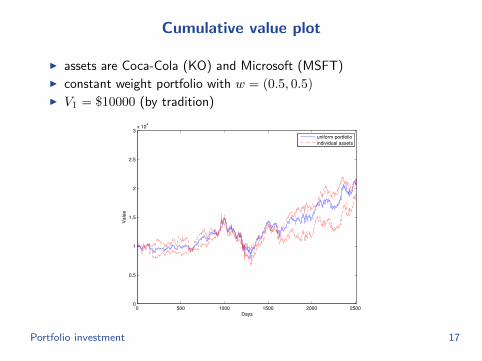
Cumulative value plot
I assets are Coca-Cola (KO) and Microsoft (MSFT)I constant weight portfolio with w = (0.5, 0.5)I V1 = $10000 (by tradition)
0 500 1000 1500 2000 25000
0.5
1
1.5
2
2.5
3x 10
4
Days
Valu
e
uniform portfolio
individual assets
Portfolio investment 17

Cumulative value plot
I w = (−3, 4)I portfolio goes bust (drops to 10% of starting value)
0 500 1000 1500 2000 25000
0.5
1
1.5
2
2.5
3x 10
4
Days
Valu
e
leveraged portfolio
individual assets
Portfolio investment 18
Outline
Return and risk
Portfolio investment
Portfolio optimization
Portfolio optimization 19
Portfolio optimization
I how should we choose the portfolio weight vector w?
I we want high (mean) portfolio return, low portfolio risk
I we know past realized asset returns but not future ones
I we will choose w that would have worked well on past returns
I . . . and hope it will work well going forward (just like data fitting)
Portfolio optimization 20

Portfolio optimization
minimize std(Rw)2 = (1/T )‖Rw − ρ1‖2
subject to 1Tw = 1, avg(Rw) = ρ
I w is the weight vector we seek
I R is the returns matrix for past returns
I Rw is the (past) portfolio return time series
I require mean (past) return ρ
I we minimize risk for specified value of return
I we are really asking what would have been the best constantallocation, had we known future returns
Portfolio optimization 21
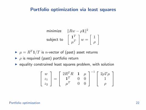
Portfolio optimization via least squares
minimize ‖Rw − ρ1‖2
subject to
[1T
µT
]w =
[1ρ
]I µ = RT1/T is n-vector of (past) asset returns
I ρ is required (past) portfolio return
I equality constrained least squares problem, with solution wz1z2
=
2RTR 1 µ1T 0 0µT 0 0
−1 2ρTµ1ρ
Portfolio optimization 22

Examples
I optimal w for annual return 1% (last asset is risk-less with 1%return)
w = (0.0000, 0.0000, 0.0000, . . . , 0.0000, 0.0000, 1.0000)
I optimal w for annual return 13%
w = (0.0250,−0.0715,−0.0454, . . . ,−0.0351, 0.0633, 0.5595)
I optimal w for annual return 25%
w = (0.0500,−0.1430,−0.0907, . . . ,−0.0703, 0.1265, 0.1191)
I asking for higher annual return yields
– more invested in risky, but high return assets– larger short positions (‘leveraging’)
Portfolio optimization 23

Cumulative value plots for optimal portfolios
cumulative value plot for optimal portfolios and some individual assets
0 500 1000 1500 2000 2500
104
105
Days
Va
lue
optimal portfolio, rho=0.20/250
optimal portfolio, rho=0.25/250
individual assets
Portfolio optimization 24
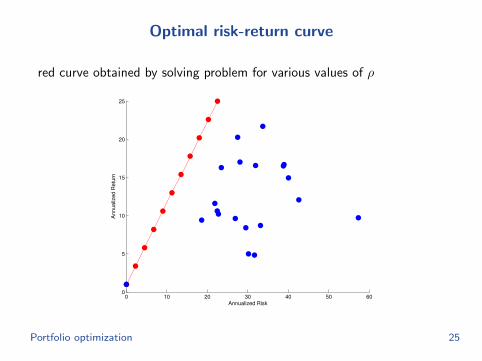
Optimal risk-return curve
red curve obtained by solving problem for various values of ρ
0 10 20 30 40 50 600
5
10
15
20
25
Annualized Risk
Annualized R
etu
rn
Portfolio optimization 25

Optimal portfolios
I perform significantly better than individual assets
I risk-return curve forms a straight line
– one end of the line is the risk-free asset
I two-fund theorem: optimal portfolio w is an affine function in ρ wz1z2
=
2RTR 1 µ1T 0 0µT 0 0
−1 RT11ρT
Portfolio optimization 26
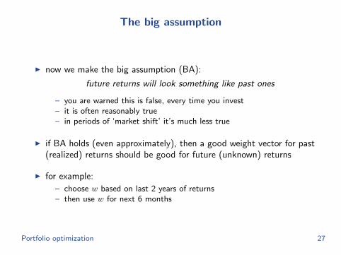
The big assumption
I now we make the big assumption (BA):
future returns will look something like past ones
– you are warned this is false, every time you invest– it is often reasonably true– in periods of ‘market shift’ it’s much less true
I if BA holds (even approximately), then a good weight vector for past(realized) returns should be good for future (unknown) returns
I for example:
– choose w based on last 2 years of returns– then use w for next 6 months
Portfolio optimization 27
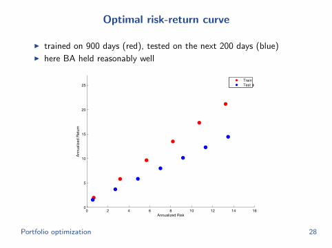
Optimal risk-return curve
I trained on 900 days (red), tested on the next 200 days (blue)I here BA held reasonably well
0 2 4 6 8 10 12 14 160
5
10
15
20
25
Annualized Risk
An
nu
alize
d R
etu
rn
Train
Test
Portfolio optimization 28
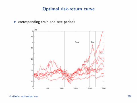
Optimal risk-return curve
I corresponding train and test periods
0 500 1000 1500 2000 25000
0.5
1
1.5
2
2.5
3
3.5
4
4.5
5x 10
4
Train Test
Portfolio optimization 29
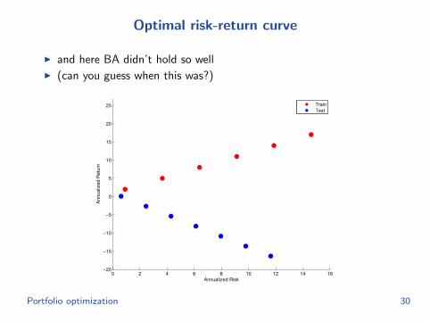
Optimal risk-return curve
I and here BA didn’t hold so wellI (can you guess when this was?)
0 2 4 6 8 10 12 14 16−20
−15
−10
−5
0
5
10
15
20
25
Annualized Risk
An
nu
alize
d R
etu
rn
Train
Test
Portfolio optimization 30
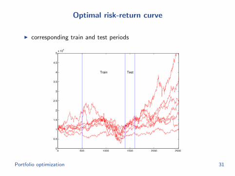
Optimal risk-return curve
I corresponding train and test periods
0 500 1000 1500 2000 25000
0.5
1
1.5
2
2.5
3
3.5
4
4.5
5x 10
4
Train Test
Portfolio optimization 31

Rolling portfolio optimization
for each period t, find weight wt using L past returns
rt−1, . . . , rt−L
variations:
I update w every K periods (say, monthly or quarterly)
I add cost term κ‖wt − wt−1‖2 to objective to discourage turnover,reduce transaction cost
I add logic to detect when the future is likely to not look like the past
I add ‘signals’ that predict future returns of assets
(. . . and pretty soon you have a quantitative hedge fund)
Portfolio optimization 32
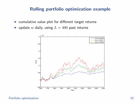
Rolling portfolio optimization example
I cumulative value plot for different target returns
I update w daily, using L = 400 past returns
1600 1700 1800 1900 2000 2100 2200 2300 2400 25000.95
1
1.05
1.1
1.15
1.2
1.25
1.3x 10
4
Days
Valu
e
rho=0.05/250
rho=0.1/250
rho=0.15/250
Portfolio optimization 33
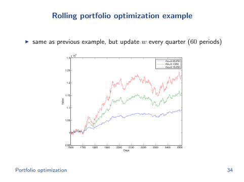
Rolling portfolio optimization example
I same as previous example, but update w every quarter (60 periods)
1600 1700 1800 1900 2000 2100 2200 2300 2400 25000.95
1
1.05
1.1
1.15
1.2
1.25
1.3x 10
4
Days
Valu
e
rho=0.05/250
rho=0.1/250
rho=0.15/250
Portfolio optimization 34