stepwise versus hierarchical regression: pros and … head: stepwise versus hierarchal regression...
TRANSCRIPT
Running head: Stepwise versus Hierarchal Regression
Stepwise versus Hierarchical Regression: Pros and Cons
Mitzi Lewis
University of North Texas
Paper presented at the annual meeting of the Southwest Educational Research Association, February 7, 2007, San Antonio.
Stepwise versus Hierarchical Regression, 2
Introduction Multiple regression is commonly used in social and
behavioral data analysis (Fox, 1991; Huberty, 1989). In
multiple regression contexts, researchers are very often
interested in determining the “best” predictors in the
analysis. This focus may stem from a need to identify
those predictors that are supportive of theory.
Alternatively, the researcher may simply be interested in
explaining the most variability in the dependent variable
with the fewest possible predictors, perhaps as part of a
cost analysis. Two approaches to determining the quality
of predictors are (1) stepwise regression and (2)
hierarchical regression. This paper will explore the
advantages and disadvantages of these methods and use a
small SPSS dataset for illustration purposes.
Stepwise Regression
Stepwise methods are sometimes used in educational and
psychological research to evaluate the order of importance
of variables and to select useful subsets of variables
(Huberty, 1989; Thompson, 1995). Stepwise regression
involves developing a sequence of linear models that,
according to Snyder (1991),
can be viewed as a variation of the forward selection
method since predictor variables are entered one at a
Stepwise versus Hierarchical Regression, 3
time, but true stepwise entry differs from forward
entry in that at each step of a stepwise analysis the
removal of each entered predictor is also considered;
entered predictors are deleted in subsequent steps if
they no longer contribute appreciable unique
predictive power to the regression when considered in
combination with newly entered predictors (Thompson,
1989). (p. 99)
Although this approach may sound appealing, it contains
inherent problems. These problems include (a) use of
degrees of freedom, (b) identification of best predictor
set of a prespecified size, and (c) replicability (Thompson,
1995).
Degrees of Freedom
Using incorrect degrees of freedom results in inflated
statistical significance levels when compared to tabled
values, a phenomenon that was found to be substantial in a
survey of published psychological research (Wilkinson,
1979). The most widely used statistical software packages
do not correctly calculate the correct degrees of freedom
in stepwise analysis, and they do not print any warning
that this is the case (Thompson, 1995; Wilkinson, 1979).
This point is emphasized by Cliff (1987) in his statement
that “most computer programs for multiple regression are
Stepwise versus Hierarchical Regression, 4
positively satanic in their temptation toward Type I errors
in this context” (p. 185).
How are these degrees of freedom incorrectly
calculated by software packages during stepwise regression?
Essentially, stepwise regression applies an F test to the
sum of squares at each stage of the procedure. Performing
multiple statistical significance tests on the same data
set as if no previous tests had been carried out can have
severe consequences on the correctness of the resulting
inferences. An appropriate analogy is given by Selvin and
Stuart (1966):
the fish which don’t fall through the net are bound to
be bigger than those which do, and it is quite
fruitless to test whether they are of average size.
Not only will this alter the performance of all
subsequent tests on the retained explanatory model –
it may destroy unbiasedness and alter mean-square-
error in estimation.” (p. 21)
However, as noted by Thompson (1995), all applications
of stepwise regression are “not equally evil regarding the
inflation of Type I error” (p. 527). Examples include
situations with (a) near zero sum of squares explained
across steps, (b) small number of predictor variables,
and/or (c) large sample size.
Stepwise versus Hierarchical Regression, 5
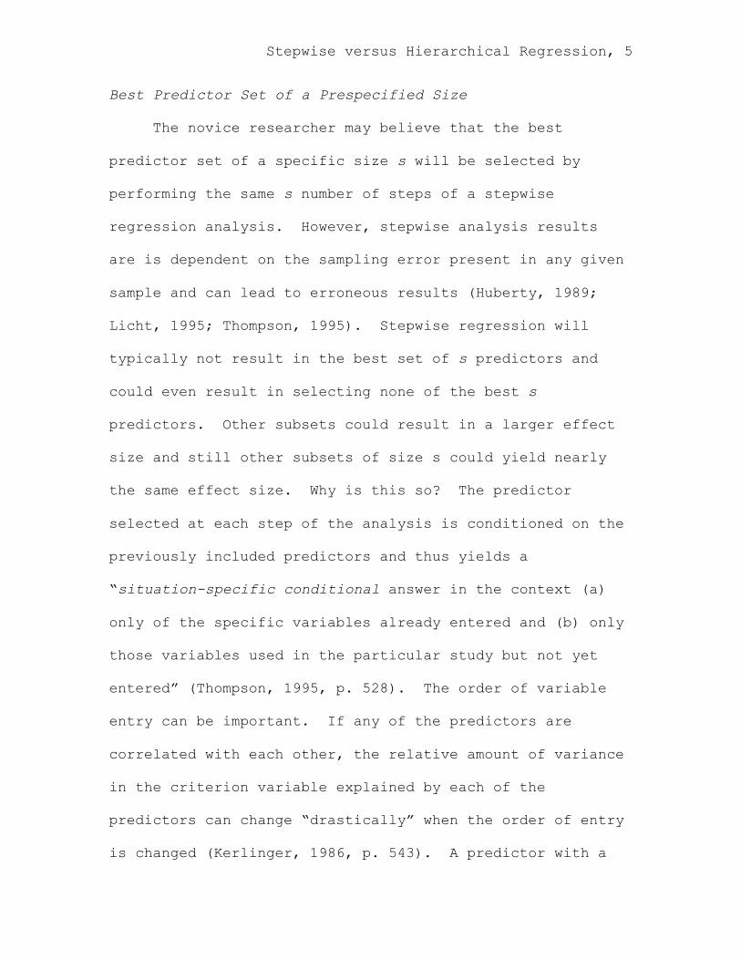
Best Predictor Set of a Prespecified Size
The novice researcher may believe that the best
predictor set of a specific size s will be selected by
performing the same s number of steps of a stepwise
regression analysis. However, stepwise analysis results
are is dependent on the sampling error present in any given
sample and can lead to erroneous results (Huberty, 1989;
Licht, 1995; Thompson, 1995). Stepwise regression will
typically not result in the best set of s predictors and
could even result in selecting none of the best s
predictors. Other subsets could result in a larger effect
size and still other subsets of size s could yield nearly
the same effect size. Why is this so? The predictor
selected at each step of the analysis is conditioned on the
previously included predictors and thus yields a
“situation-specific conditional answer in the context (a)
only of the specific variables already entered and (b) only
those variables used in the particular study but not yet
entered” (Thompson, 1995, p. 528). The order of variable
entry can be important. If any of the predictors are
correlated with each other, the relative amount of variance
in the criterion variable explained by each of the
predictors can change “drastically” when the order of entry
is changed (Kerlinger, 1986, p. 543). A predictor with a
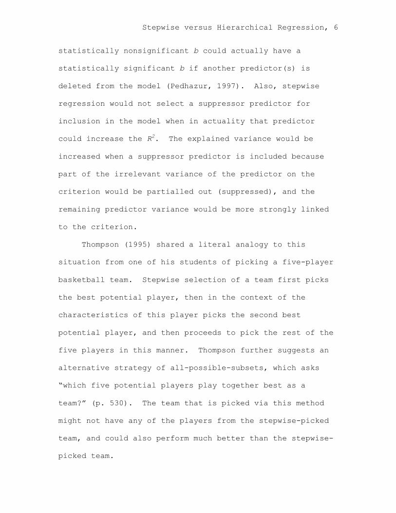
Stepwise versus Hierarchical Regression, 6
statistically nonsignificant b could actually have a
statistically significant b if another predictor(s) is
deleted from the model (Pedhazur, 1997). Also, stepwise
regression would not select a suppressor predictor for
inclusion in the model when in actuality that predictor
could increase the R2. The explained variance would be
increased when a suppressor predictor is included because
part of the irrelevant variance of the predictor on the
criterion would be partialled out (suppressed), and the
remaining predictor variance would be more strongly linked
to the criterion.
Thompson (1995) shared a literal analogy to this
situation from one of his students of picking a five-player
basketball team. Stepwise selection of a team first picks
the best potential player, then in the context of the
characteristics of this player picks the second best
potential player, and then proceeds to pick the rest of the
five players in this manner. Thompson further suggests an
alternative strategy of all-possible-subsets, which asks
“which five potential players play together best as a
team?” (p. 530). The team that is picked via this method
might not have any of the players from the stepwise-picked
team, and could also perform much better than the stepwise-
picked team.
Stepwise versus Hierarchical Regression, 7
A colleague of the present author noted that one could
also imagine a different type of team being brought
together to work on a common goal. For example, a team of
the smartest people in an organization might be selected in
a stepwise manner to produce a report of cutting edge
research in their field. These highly intelligent people
might be, for example, Professor B. T. Weight, Professor S.
T. Coefficient, Professor E. F. Size, and Professor C. R.
Lation. Although these people may be the most intelligent
people in the organization, they may not be the group of
people who could produce the best possible report if they
do not work together well. Perhaps personality conflicts,
varying philosophies, or egos might interfere with the
group being able to work together effectively. It could be
that using an all-possible-subsets approach, or a
hierarchical regression approach (see subsequent
discussion), would result in a totally different group of
individuals since these approaches would also consider how
different combinations of individuals work together as a
team. This new team might then be the one that would
produce the best possible report because they do not have
the previously mentioned issues and as a result work
together more successfully as a team. (Disclaimer: any
Stepwise versus Hierarchical Regression, 8
resemblance of these fictional team members to actual
people is purely a coincidence.)
Replicability
Stepwise regression generally does not result in
replicable conclusions due to its dependence on sampling
error (Copas, 1983; Fox, 1991; Gronnerod, 1006; Huberty,
1989; Menard, 1995; Pedhazur, 1991; Thompson, 1995). As
stated by Menard (1995), the use of stepwise procedures
“capitalizes on random variations in the data and produces
results that tend to be idosyncratic and difficult to
replicate in any sample other than the sample in which they
were originally obtained" (p. 54) and therefore results
should be regarded as “inconclusive” (p. 57). As variable
determinations are made at each step, there may be
instances in which one variable is chosen over another due
to a small difference in predictive ability. This small
difference, which could be due to sampling error, impacts
each subsequent step. Thompson (1995) likens these linear-
series decisions to decisions that are made when working
through a maze. Once a decision is made to turn one way
instead of another, a whole sequence of decisions (and
therefore results) are no longer possible.
This difficulty of sampling error, and thus the
possible impact of sampling error on the analysis, could be
Stepwise versus Hierarchical Regression, 9
estimated using cross-validation (Fox, 1991; Henderson &
Valleman, 1981; Tabachnick & Fidell, 1996) or other
techniques. Sampling error is less problematic with (a)
fewer predictor variables, (b) larger effect sizes, and (c)
larger sample sizes (Thompson, 1995). Also, sampling error
is less of an issue when the regressor values for the
predicted data will be used “within the configuration for
which selection was employed” (e.g., as in a census
undercount) (Fox, 1991, p. 19).
Hierarchical Regression
One alternative to stepwise regression is hierarchical
regression. Hierarchical regression can be useful for
evaluating the contributions of predictors above and beyond
previously entered predictors, as a means of statistical
control, and for examining incremental validity. Like
stepwise regression, hierarchical regression is a
sequential process involving the entry of predictor
variables into the analysis in steps. Unlike stepwise
regression, the order of variable entry into the analysis
is based on theory. Instead of letting a computer software
algorithm “choose” the order in which to enter the
variables, these order determinations are made by the
researcher based on theory and past research. As Kerlinger
(1986) noted, while there is no “correct” method for
Stepwise versus Hierarchical Regression, 10
choosing order of variable entry, there is also “no
substitute for depth of knowledge of the research
problem . . . the research problem and the theory behind
the problem should determine the order of entry of
variables in multiple regression analysis” (p. 545).
Stated another way by Fox (1991), ”mechanical model-
selection and modification procedures . . . generally
cannot compensate for weaknesses in the data and are no
substitute for judgment and thought” (p. 21). Simply put,
“the data analyst knows more than the computer” (Henderson
& Velleman, 1981, p. 391).
Hierarchical regression is an appropriate tool for
analysis when variance on a criterion variable is being
explained by predictor variables that are correlated with
each other (Pedhazur, 1997). Since correlated variables
are commonly seen in social sciences research and are
especially prevalent in educational research, this makes
hierarchical regression quite useful. Hierarchical
regression is a popular method used to analyze the effect
of a predictor variable after controlling for other
variables. This “control” is achieved by calculating the
change in the adjusted R2 at each step of the analysis, thus
accounting for the increment in variance after each
Stepwise versus Hierarchical Regression, 11
variable (or group of variables) is entered into the
regression model (Pedhazur, 1997).
Just a few recent examples of hierarchical regression
analysis use in research include:
1. Reading comprehension: To assess the unique
proportion of variance of listening
comprehension and decoding ability on first and
second grade children’s reading comprehension
(Megherbi, Seigneuric, & Ehrlich, 2006).
2. Adolescent development: To assess the unique
proportion of variance of parental attachment
and social support to college students’
adjustment following a romantic relationship
breakup (Moller, Fouladi, McCarthy, & Hatch,
2003).
3. Reading Disability: To assess the unique
proportion of variance of visual-orthographic
skills on reading abilities (Badian, 2005).
4. School Counselor Burnout: To assess the unique
proportion of variance of demographic,
intrapersonal, and organizational factors on
school counselor burnout (Wilkerson & Bellini,
2006).
Stepwise versus Hierarchical Regression, 12
5. College Student Alcohol Use: To assess the
unique proportion of variance of sensation
seeking and peer influence on college students’
drinking behaviors (Yanovitky, 2006).
6. Children with Movement Difficulties in Physical
Education: To examine effects of motivational
climate and perceived competence on
participation behaviors of children with
movement difficulties in physical education
(Dunn & Dunn, 2006).
Another reason that hierarchical regression is the
analysis tool of choice in so many research scenarios is
that it does not have the same drawbacks of stepwise
regression regarding degrees of freedom, identification of
best predictor set of a prespecified size, and
replicability.
Degrees of Freedom
Degrees of freedom for hierarchical regression are
correctly displayed in many of the statistical software
packages that do not display the correct degrees of freedom
for stepwise regression. This is because in hierarchical
regression, the degrees of freedom correctly reflect the
number of statistical tests that have been made to arrive
at the resulting model. Degrees of freedom utilized by
Stepwise versus Hierarchical Regression, 13
many software packages in stepwise regression analysis do
not correctly reflect the number of statistical tests that
have been made to arrive at the resulting model; instead
the degrees of freedom are under calculated. Thus,
statistical significance levels displayed in hierarchical
regression output are correct and statistical significance
levels displayed in stepwise regression output are inflated,
resulting in inflated chances for Type I errors.
Best Predictor Set of a Prespecified Size
Hierarchical regression analysis involves choosing a
best predictor set interactively between computer and the
researcher. The order of variable entry is determined by
the researcher before the analysis is conducted. In this
manner, decisions are based on theory and research instead
of being made arbitrarily, in blind automation, by the
computer (as they are in stepwise regression; Henderson &
Vellman, 1981).
Replicability
Like stepwise regression, hierarchical regression is
also subject to problems associated with sampling error.
However, the likelihood of these problems is reduced by
interaction of the researcher with the data. For example,
instead of one variable being chosen over another variable
due to a small difference in predictive ability, the order
Stepwise versus Hierarchical Regression, 14
of variable entry is chosen by the researcher. Thus,
results from an arbitrary decision that is more likely to
reflect sampling error (in the case of stepwise regression)
are instead results based on researcher expertise (in the
case of hierarchical regression). Of course, remaining
sampling error can still be estimated via cross-validation
or other techniques. And again, sampling error will be
less of an issue the larger the sample size and effect size,
and the fewer the predictor variables.
Heuristic SPSS Example
Stepwise Regression
As previously discussed, stepwise regression involves
developing a sequence of linear models through variable
entry as determined by computer algorithms. A heuristic
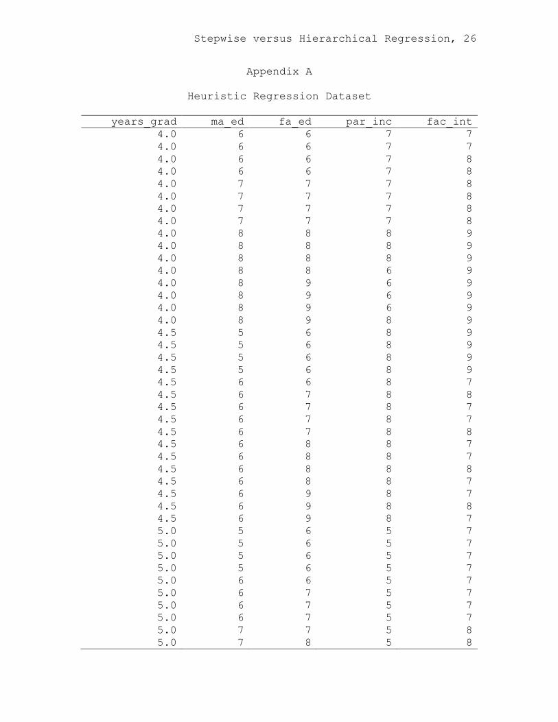
SPSS dataset has been constructed (Appendix A) and will be
analyzed for illustration purposes. Syntax is provided in
Appendix B.
Stepwise regression was used to regress mother’s
education level (ma_ed), father’s education level (fa_ed),
parent’s income (par_inc), and faculty interaction level
(fac_int) on years to graduation (years_grad). Inspection
of correlations between the variables (Table 1) reveal (a)
that mother’s education, parent’s income, and faculty
interaction are all highly correlated with years to
Stepwise versus Hierarchical Regression, 15
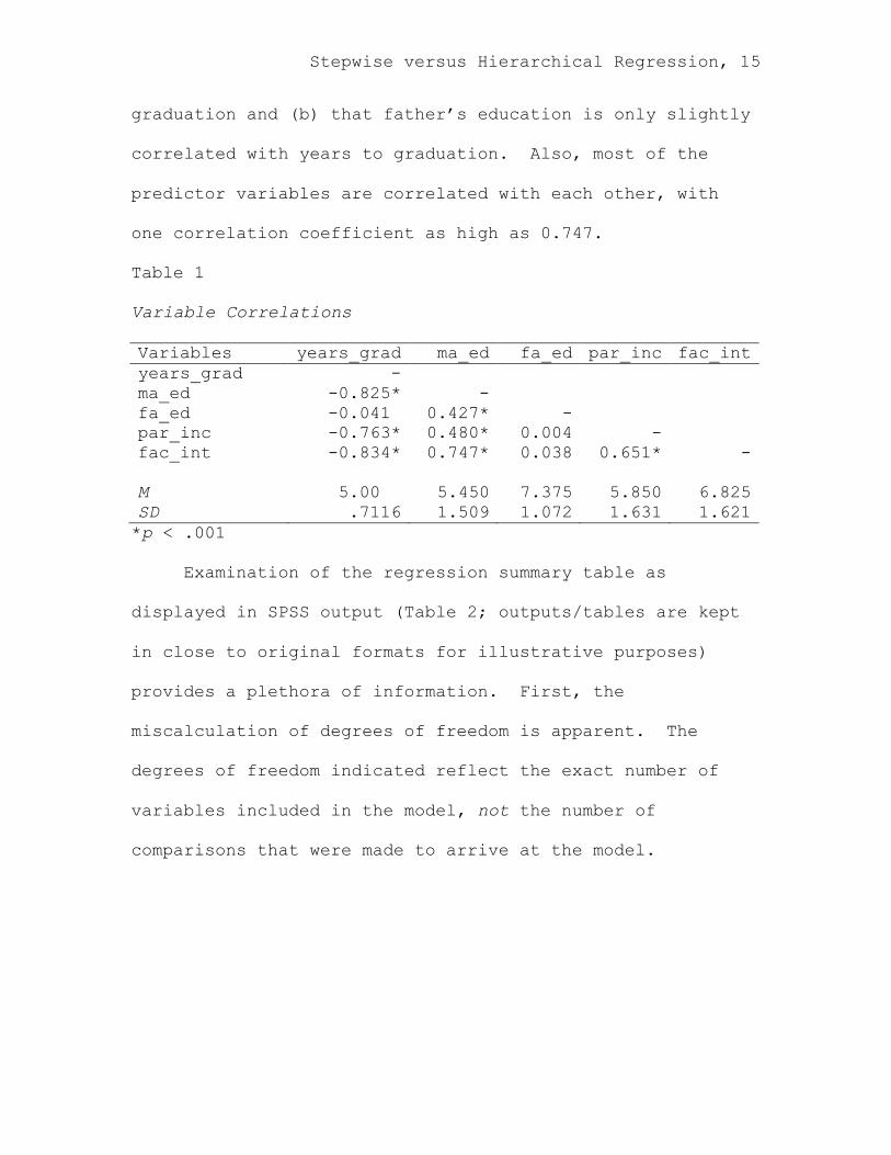
graduation and (b) that father’s education is only slightly
correlated with years to graduation. Also, most of the
predictor variables are correlated with each other, with
one correlation coefficient as high as 0.747.
Table 1
Variable Correlations
Variables years_grad ma_ed fa_ed par_inc fac_int years_grad - ma_ed -0.825* - fa_ed -0.041* 0.427* - par_inc -0.763* 0.480* 0.004 - fac_int -0.834* 0.747* 0.038 0.651* - M 5.000* 5.450 7.375 5.850 6.825 SD .7116 1.509 1.072 1.631 1.621 *p < .001
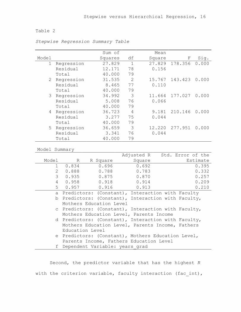
Examination of the regression summary table as
displayed in SPSS output (Table 2; outputs/tables are kept
in close to original formats for illustrative purposes)
provides a plethora of information. First, the
miscalculation of degrees of freedom is apparent. The
degrees of freedom indicated reflect the exact number of
variables included in the model, not the number of
comparisons that were made to arrive at the model.
Stepwise versus Hierarchical Regression, 16
Table 2
Stepwise Regression Summary Table
Model Sum of
Squares df Mean
Square F Sig. 1 Regression 27.829 1 27.829 178.356 0.000
Residual 12.171 78 0.156 Total 40.000 79
2 Regression 31.535 2 15.767 143.423 0.000 Residual 8.465 77 0.110 Total 40.000 79
3 Regression 34.992 3 11.664 177.027 0.000 Residual 5.008 76 0.066 Total 40.000 79
4 Regression 36.723 4 9.181 210.146 0.000 Residual 3.277 75 0.044 Total 40.000 79
5 Regression 36.659 3 12.220 277.951 0.000 Residual 3.341 76 0.044 Total 40.000 79 Model Summary
Model R R Square Adjusted R
Square Std. Error of the
Estimate 1 0.834 0.696 0.692 0.395 2 0.888 0.788 0.783 0.332 3 0.935 0.875 0.870 0.257 4 0.958 0.918 0.914 0.209 5 0.957 0.916 0.913 0.210 a Predictors: (Constant), Interaction with Faculty b Predictors: (Constant), Interaction with Faculty, Mothers Education Level
c Predictors: (Constant), Interaction with Faculty, Mothers Education Level, Parents Income
d
Predictors: (Constant), Interaction with Faculty, Mothers Education Level, Parents Income, Fathers Education Level
e Predictors: (Constant), Mothers Education Level, Parents Income, Fathers Education Level
f Dependent Variable: years_grad
Second, the predictor variable that has the highest R
with the criterion variable, faculty interaction (fac_int),
Stepwise versus Hierarchical Regression, 17
is the first variable entered into the analysis. However,
the final model of the analysis (model 5/e) does not
include the faculty interaction variable. Thus, stepwise
regression egregiously results in a model that does not
include the predictor variable that has the highest
correlation with the criterion variable.
Because the significance tests displayed in the output
of the stepwise regression analysis do not approximate the
probability that the resulting model will actually
represent future samples, another method is needed to
estimate replicability. Double cross-validation is
performed to achieve this objective. The resulting double
cross-validation coefficients are 0.999. Upon initial
reflection, these findings may seem quite high, but in
consideration of the unusually elevated R in these analyses
(0.954 & 0.961), the findings are not so surprising. Had
the R values been lower or had a larger number of predictor
variables been included in the analysis, smaller double-
cross validation coefficients would have been expected.
Hierarchical Regression
The dataset utilized to illustrate some of the
concepts involved with stepwise regression can also be used
to demonstrate hierarchical regression. Variable selection
for the hierarchical regression analysis will be based on

Stepwise versus Hierarchical Regression, 18
theory. It is generally understood that a number of
factors contribute to the level of college student success
(years_grad), including parent’s education level (ma_ed and
fa_ed), socioeconomic status (par_inc), and amount of
interaction with faculty members (fac_int). Hierarchical
regression will be employed to determine if the amount of
student interaction with faculty members contributes a
unique proportion of variance to student success
(years_grad).
To “control” for student characteristics of parent’s
education level and socioeconomic status, these variables
will be entered into the first block of the analysis.
Fac_int will be entered into the second block of the
analysis to determine its unique contribution to variance
explained of years to graduation. Note that (a) variable
entry into these “blocks” can occur one variable at a time
or as a group (or block) or variables and (b) these
determinations are made by the researcher.
Examination of the regression summary table (Table 3)
again provides much information. First, since the
researcher selected the specific variables for analysis,
the degrees of freedom correctly reflect the number of
comparisons that were made to arrive at the models.
Stepwise versus Hierarchical Regression, 19
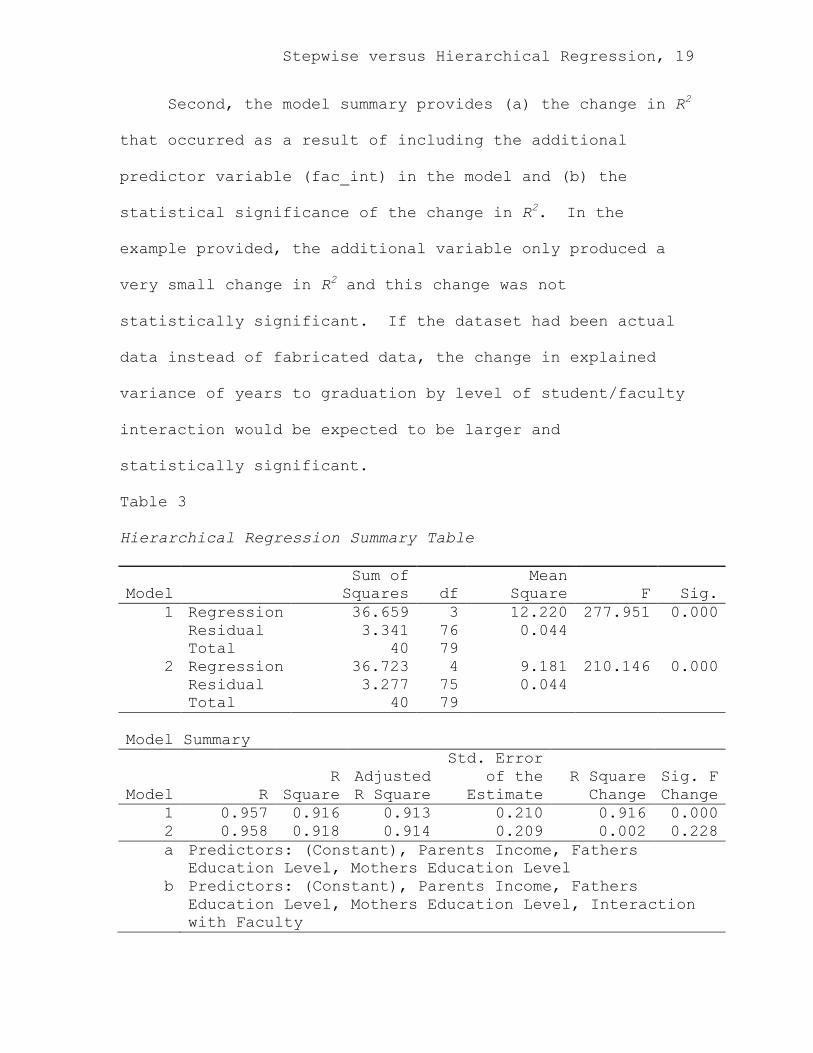
Second, the model summary provides (a) the change in R2
that occurred as a result of including the additional
predictor variable (fac_int) in the model and (b) the
statistical significance of the change in R2. In the
example provided, the additional variable only produced a
very small change in R2 and this change was not
statistically significant. If the dataset had been actual
data instead of fabricated data, the change in explained
variance of years to graduation by level of student/faculty
interaction would be expected to be larger and
statistically significant.
Table 3
Hierarchical Regression Summary Table
Model Sum of
Squares df Mean
Square F Sig. 1 Regression 36.659 3 12.220 277.951 0.000
Residual 3.341 76 0.044 Total 40 79
2 Regression 36.723 4 9.181 210.146 0.000 Residual 3.277 75 0.044 Total 40 79 Model Summary
Model R R
Square Adjusted R Square
Std. Error of the
Estimate R Square
Change Sig. F Change
1 0.957 0.916 0.913 0.210 0.916 0.000 2 0.958 0.918 0.914 0.209 0.002 0.228 a Predictors: (Constant), Parents Income, Fathers Education Level, Mothers Education Level
b
Predictors: (Constant), Parents Income, Fathers Education Level, Mothers Education Level, Interaction with Faculty
Stepwise versus Hierarchical Regression, 20
Again, the adjusted R2 would indicate that sampling error
does not have much impact on the present scenario, probably
because of the high effect size and the small number of
predictor variables. If the effect size were lower and/or
the number of predictor variables increased, the adjusted R2
would probably provide a larger theoretical correction for
these issues, and this correction could be further examined
by cross-validation or other techniques.
Conclusion
Selecting the appropriate statistical tool for
analysis is dependent upon the intended use of the analysis.
As Pedhazur (1997) stated,
Practical considerations in the selection of
specific predictors may vary, depending on the
circumstances of the study, the researcher’s
specific aims, resources, and frame of reference,
to name some. Clearly, it is not possible to
develop a systematic selection method that would
take such considerations into account. (p. 211)
This rationale is in conflict with the automated, algorithm
based analysis of stepwise regression. Nonetheless, there
are still instances where stepwise regression has been
recommended for use: in exploratory, predictive research
(Menard, 1995). Even in this case, stepwise regression
Stepwise versus Hierarchical Regression, 21
might not yield the largest R2 because it would ignore
suppressor variables.
Therefore, while intended use is a critical factor for
choosing a statistical analysis tool, the problems
associated with stepwise regression suggest that extreme
caution should be taken if it is selected. Specifically,
one could lessen the issues connected with stepwise
regression analysis if it were not selected in instances
with smaller samples, smaller effect sizes, and more
predictor variables. Even then, interpretation of results
should only be preliminary and they should not include (a)
assigning meaningfulness to the order of variable entry and
selection or (b) assuming optimality of the resulting
subset of variables. To emphasize, Pedhazur (1997) noted
“the pairing of model construction, whose very essence is a
theoretical framework . . . with predictor-selection
procedures that are utterly atheoretical is deplorable” (p.
211).
Stepwise versus Hierarchical Regression, 22
References
Badian, N. A. (2005). Does a visual-orthographic deficit
contribute to reading disability? Annals of Dyslexia,
55(1), 28-52.
Cliff, N. (1987). Analyzing multivariate data. New York:
Harcourt Brace Jovanovich.
Copas, J. B. (1983). Regression, prediction, and shrinkage.
J. R. Statist. Soc. B, 45, 311-354.
Dunn, J. C., & Dunn, J. G. (2006). Psychosocial
determinants of physical education behavior in
children with movement difficulties. Adapted Physical
Activity Quarterly, 23, 293-309.
Fox, J. (1991). Regression diagnostics: An introduction.
Sage University Paper series on Quantitative
Applications in the Social Sciences, series no. 07-079.
Newbury Park, CA: Sage.
Gronnerod, C. (2006). Reanalysis of the Gronnerod (2003)
Rorschach Temporal Stability Meta-Analysis Data Set.
Journal of Personality Assessment, 86, 222-225.
Henderson, H. V., & Velleman, P. F. (1981). Building
multiple regression models interactively. Biometrics,
37, 391 – 411.

Stepwise versus Hierarchical Regression, 23
Huberty, C. J (1989). Problems with stepwise methods-better
alternatives. In B. Thompson (Ed.), Advances in social
science methodology (Vol. 1, pp. 43-70). Greenwich, CT:
JAI Press.
Kerlinger, F. N. (1986). Foundations of behavioral research
(3rd ed.). New York: Holt, Rinehart and Winston.
Licht, M. H. (1995). Multiple regression and correlation.
In L. G. Grimm & P. R. Yarnold (Eds.), Reading and
understanding multivariate statistics. Washington, DC:
American Psychological Association.
Megherbi, H., Seigneuric, A., & Ehrlich, M. (2006).
Reading omprehension in French 1st and 2nd grade
children: Contribution of decoding and language
comprehension. European Journal of Psychology of
Education, 21, 135-137.
Menard, S. (1995). Applied logistic regression analysis.
Sage University Paper series on Quantitative
Applications in the Social Sciences, series no. 07-106.
Thousand Oaks, CA: Sage.
Moller, N. P., Roulandi, R. T., McCarthy, C. J., & Hatch, K.
D. (2003). Relationship of attachment and social
support to college students’ adjustment following a
relationship breakup. Journal of Counseling &
Development, 81(3), 354-369.
Stepwise versus Hierarchical Regression, 24
Pedhazur, E. J. (1997). Multiple regression in behavioral
research (3rd ed.). Orlando, FL: Harcourt Brace.
Selvin, H. C., & Stuart, A. (1966). Data-dredging
procedures in survey analysis. The American
Statistician, 20(3), 20-23.
Snyder, P. (1991). Three reasons why stepwise regression
methods should not be used by researchers. In B.
Thompson (Ed.), Advances in social science methodology
(Vol. 1, pp. 99-105). Greenwich, CT: JAI Press.
SPSS for Windows, Rel. 14.0.0. (2005). Chicago: SPSS Inc.
Tabachnick, B. G., & Fidell, L. S. (1996). Using
multivariate statistics (3rd ed.). New York: Harper
Collins.
Thompson, B. (1989). Why won’t stepwise methods die?
Measurement and Evaluation in Counseling and
Development, 21(4), 146-148.
Thompson, B. (1995). Stepwise regression and stepwise
discriminant analysis need not apply here: A
guidelines editorial. Educational and Psychological
Measurement, 55, 525-534.
Wilkerson, K., & Bellini, J. (2006). Intrapersonal and
organizational factors associated with burnout among
school counselors. Journal of Counseling &
Development, 84, 440-450.
Stepwise versus Hierarchical Regression, 25
Wilkinson, L. (1979). Tests of significance in stepwise
regression. Psychological Bulletin, 86, 168-174.
Yanovitzky, I. (2006). Sensation seeking an alcohol use by
college students: Examining multiple pathways of
effects. Journal of Health Communication, 11, 269-280.
Stepwise versus Hierarchical Regression, 26
Appendix A
Heuristic Regression Dataset
years_grad ma_ed fa_ed par_inc fac_int 4.0 6 6 7 7 4.0 6 6 7 7 4.0 6 6 7 8 4.0 6 6 7 8 4.0 7 7 7 8 4.0 7 7 7 8 4.0 7 7 7 8 4.0 7 7 7 8 4.0 8 8 8 9 4.0 8 8 8 9 4.0 8 8 8 9 4.0 8 8 6 9 4.0 8 9 6 9 4.0 8 9 6 9 4.0 8 9 6 9 4.0 8 9 8 9 4.5 5 6 8 9 4.5 5 6 8 9 4.5 5 6 8 9 4.5 5 6 8 9 4.5 6 6 8 7 4.5 6 7 8 8 4.5 6 7 8 7 4.5 6 7 8 7 4.5 6 7 8 8 4.5 6 8 8 7 4.5 6 8 8 7 4.5 6 8 8 8 4.5 6 8 8 7 4.5 6 9 8 7 4.5 6 9 8 8 4.5 6 9 8 7 5.0 5 6 5 7 5.0 5 6 5 7 5.0 5 6 5 7 5.0 5 6 5 7 5.0 6 6 5 7 5.0 6 7 5 7 5.0 6 7 5 7 5.0 6 7 5 7 5.0 7 7 5 8 5.0 7 8 5 8
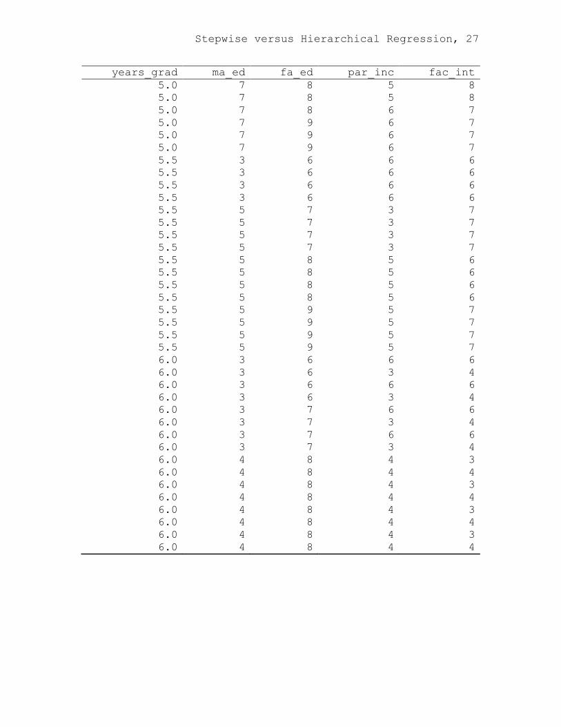
Stepwise versus Hierarchical Regression, 27
years_grad ma_ed fa_ed par_inc fac_int 5.0 7 8 5 8 5.0 7 8 5 8 5.0 7 8 6 7 5.0 7 9 6 7 5.0 7 9 6 7 5.0 7 9 6 7 5.5 3 6 6 6 5.5 3 6 6 6 5.5 3 6 6 6 5.5 3 6 6 6 5.5 5 7 3 7 5.5 5 7 3 7 5.5 5 7 3 7 5.5 5 7 3 7 5.5 5 8 5 6 5.5 5 8 5 6 5.5 5 8 5 6 5.5 5 8 5 6 5.5 5 9 5 7 5.5 5 9 5 7 5.5 5 9 5 7 5.5 5 9 5 7 6.0 3 6 6 6 6.0 3 6 3 4 6.0 3 6 6 6 6.0 3 6 3 4 6.0 3 7 6 6 6.0 3 7 3 4 6.0 3 7 6 6 6.0 3 7 3 4 6.0 4 8 4 3 6.0 4 8 4 4 6.0 4 8 4 3 6.0 4 8 4 4 6.0 4 8 4 3 6.0 4 8 4 4 6.0 4 8 4 3 6.0 4 8 4 4
Stepwise versus Hierarchical Regression, 28
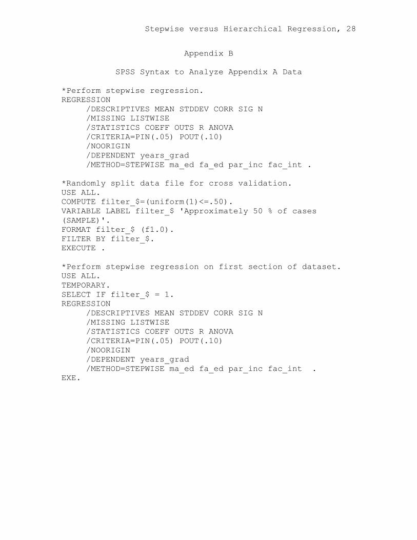
Appendix B
SPSS Syntax to Analyze Appendix A Data
*Perform stepwise regression. REGRESSION /DESCRIPTIVES MEAN STDDEV CORR SIG N /MISSING LISTWISE /STATISTICS COEFF OUTS R ANOVA /CRITERIA=PIN(.05) POUT(.10) /NOORIGIN /DEPENDENT years_grad /METHOD=STEPWISE ma_ed fa_ed par_inc fac_int . *Randomly split data file for cross validation. USE ALL. COMPUTE filter_$=(uniform(1)<=.50). VARIABLE LABEL filter_$ 'Approximately 50 % of cases (SAMPLE)'. FORMAT filter_$ (f1.0). FILTER BY filter_$. EXECUTE . *Perform stepwise regression on first section of dataset. USE ALL. TEMPORARY. SELECT IF filter_$ = 1. REGRESSION /DESCRIPTIVES MEAN STDDEV CORR SIG N /MISSING LISTWISE /STATISTICS COEFF OUTS R ANOVA /CRITERIA=PIN(.05) POUT(.10) /NOORIGIN /DEPENDENT years_grad /METHOD=STEPWISE ma_ed fa_ed par_inc fac_int . EXE.
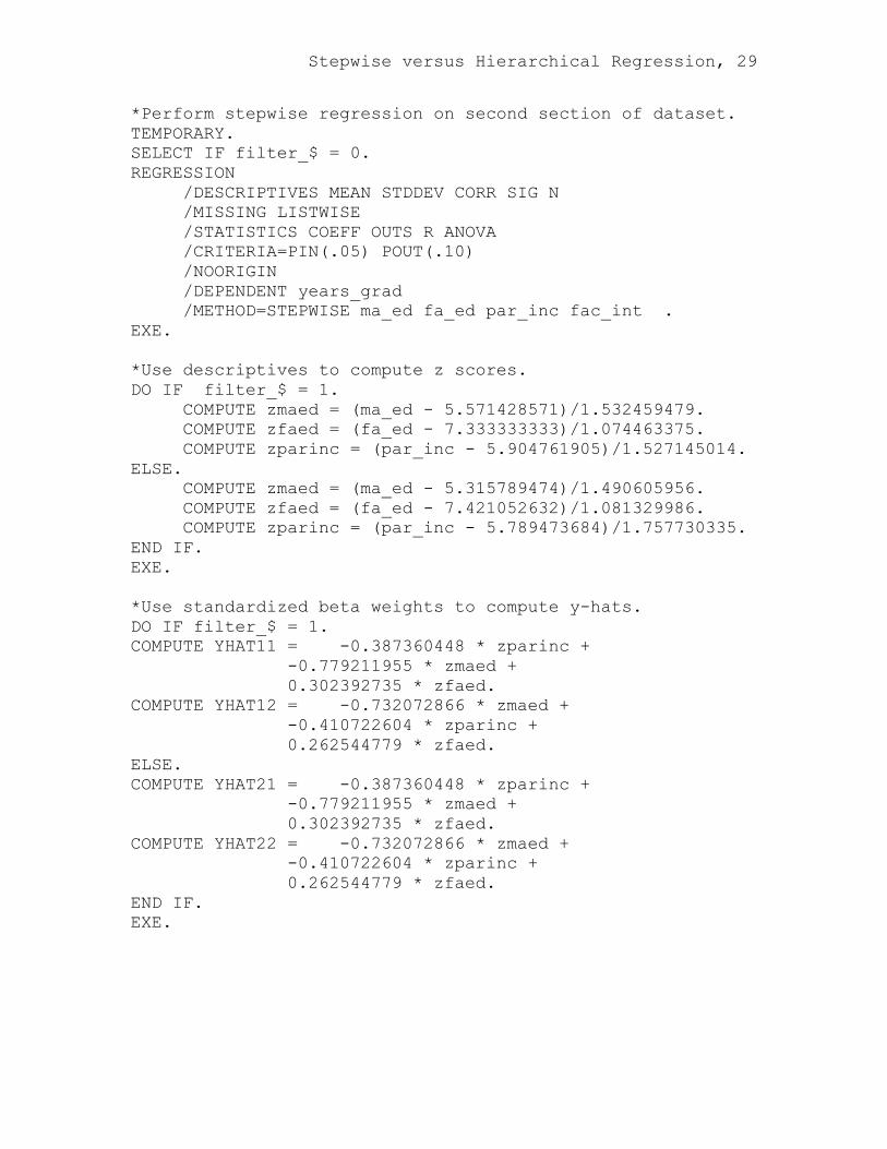
Stepwise versus Hierarchical Regression, 29
*Perform stepwise regression on second section of dataset. TEMPORARY. SELECT IF filter_$ = 0. REGRESSION /DESCRIPTIVES MEAN STDDEV CORR SIG N /MISSING LISTWISE /STATISTICS COEFF OUTS R ANOVA /CRITERIA=PIN(.05) POUT(.10) /NOORIGIN /DEPENDENT years_grad /METHOD=STEPWISE ma_ed fa_ed par_inc fac_int . EXE. *Use descriptives to compute z scores. DO IF filter_$ = 1. COMPUTE zmaed = (ma_ed - 5.571428571)/1.532459479. COMPUTE zfaed = (fa_ed - 7.333333333)/1.074463375. COMPUTE zparinc = (par_inc - 5.904761905)/1.527145014. ELSE. COMPUTE zmaed = (ma_ed - 5.315789474)/1.490605956. COMPUTE zfaed = (fa_ed - 7.421052632)/1.081329986. COMPUTE zparinc = (par_inc - 5.789473684)/1.757730335. END IF. EXE. *Use standardized beta weights to compute y-hats. DO IF filter_$ = 1. COMPUTE YHAT11 = -0.387360448 * zparinc + -0.779211955 * zmaed + 0.302392735 * zfaed. COMPUTE YHAT12 = -0.732072866 * zmaed + -0.410722604 * zparinc + 0.262544779 * zfaed. ELSE. COMPUTE YHAT21 = -0.387360448 * zparinc + -0.779211955 * zmaed + 0.302392735 * zfaed. COMPUTE YHAT22 = -0.732072866 * zmaed + -0.410722604 * zparinc + 0.262544779 * zfaed. END IF. EXE.
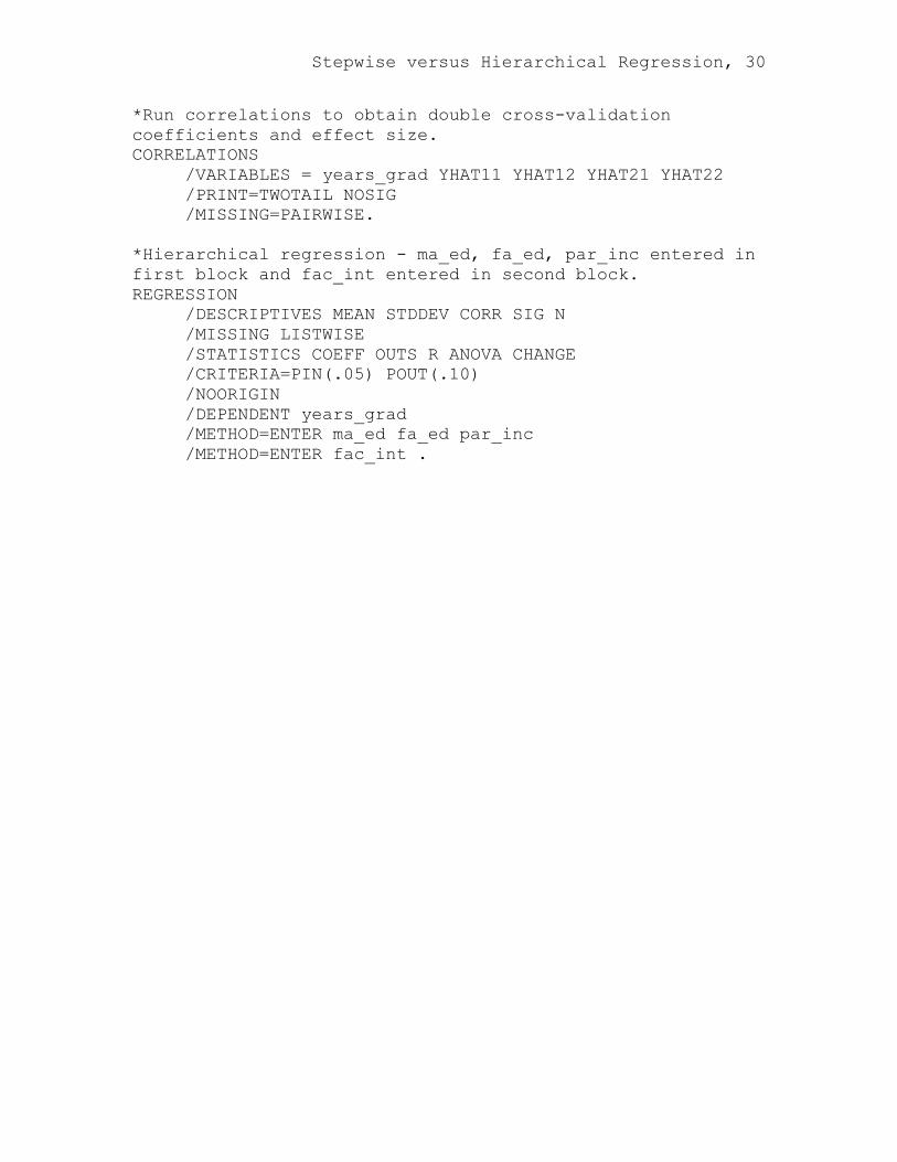
Stepwise versus Hierarchical Regression, 30
*Run correlations to obtain double cross-validation coefficients and effect size. CORRELATIONS /VARIABLES = years_grad YHAT11 YHAT12 YHAT21 YHAT22 /PRINT=TWOTAIL NOSIG /MISSING=PAIRWISE. *Hierarchical regression - ma_ed, fa_ed, par_inc entered in first block and fac_int entered in second block. REGRESSION /DESCRIPTIVES MEAN STDDEV CORR SIG N /MISSING LISTWISE /STATISTICS COEFF OUTS R ANOVA CHANGE /CRITERIA=PIN(.05) POUT(.10) /NOORIGIN /DEPENDENT years_grad /METHOD=ENTER ma_ed fa_ed par_inc /METHOD=ENTER fac_int .