stereo matching - 國立臺灣大學media.ee.ntu.edu.tw/courses/cv/18f/slides/cv2018_lec14.pdf ·...
TRANSCRIPT

Stereo MatchingWei-Chih Tu (塗偉志)
National Taiwan University
Fall 2018
Computer Vision: from Recognition to GeometryLecture 14

Stereo Matching
• For pixel 𝑥0 in one image, where is the corresponding point 𝑥1 in another image?• Stereo: two or more input views
• Based on the epipolar geometry, corresponding points lie on the epipolar lines• A matching problem
2

Epipolar Geometry for Converging Cameras
• Still difficult• Need to trace different epipolar lines for every point
3

Image Rectification
4

Image Rectification
• Reproject image planes onto a common plane parallel to the line between optical centers
• Pixel motion is horizontal after this transformation
• Two homographies(3x3 transform), one for each image
5

Image Rectification
• [Loop and Zhang 1999]
6Loop and Zhang. Computing Rectifying Homographies for Stereo Vision. In CVPR 1999.
Original image pair overlaid with several epipolar lines.
Images transformed so that epipolarlines are parallel.
Images rectified so that epipolar lines are horizontal and aligned in vertical.
Final rectification that minimizes horizontal distortions. (Shearing)

Disparity Estimation
• After rectification, stereo matching becomes the disparity estimation problem
• Disparity = horizontal displacement of corresponding points in the two images• Disparity of = 𝑥𝐿 − 𝑥𝑅
7
𝑥𝐿 𝑥𝑅

Disparity Estimation
• The “hello world” algorithm: block matching• Consider SSD as matching cost
8
Left view Right view
𝑑 0 1 2 3 … 33 … 59 60
SSD 100 90 88 88 … 12 … 77 85
Winner take all (WTA)

Disparity Estimation
• The “hello world” algorithm: block matching
• For each pixel in the left image
• For each disparity level
• For each pixel in window
• Compute matching cost
• Find disparity with minimum matching cost
9
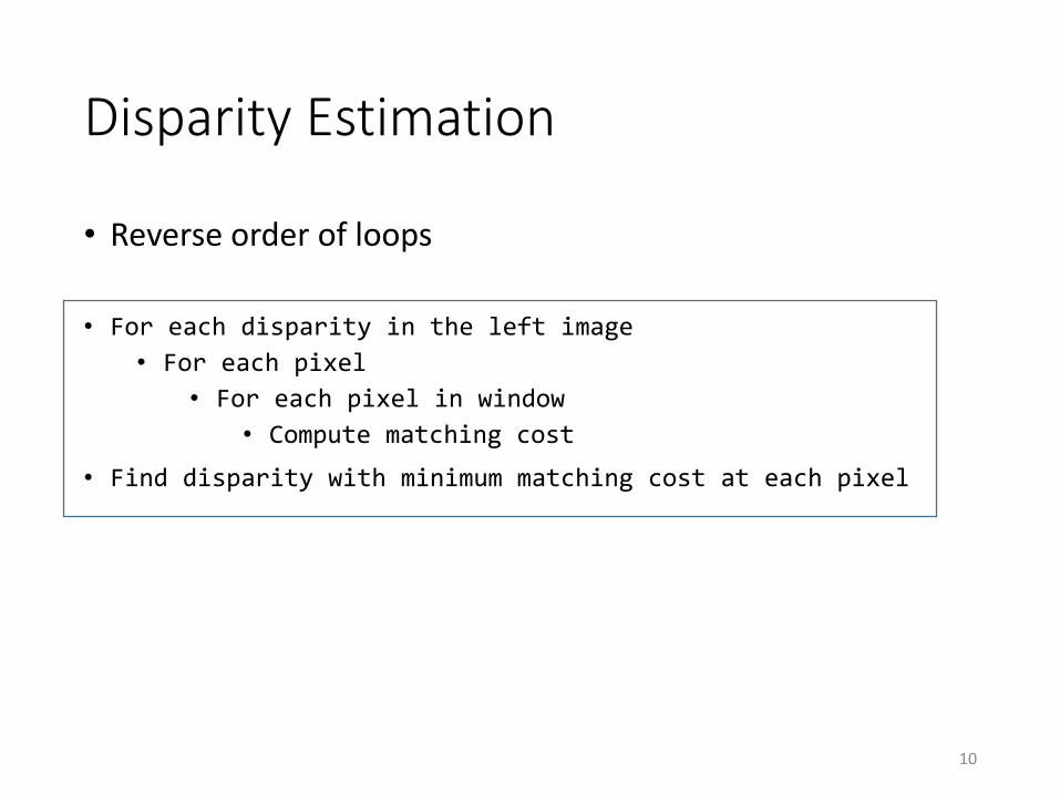
Disparity Estimation
• Reverse order of loops
• For each disparity in the left image
• For each pixel
• For each pixel in window
• Compute matching cost
• Find disparity with minimum matching cost at each pixel
10
Disparity Estimation
11
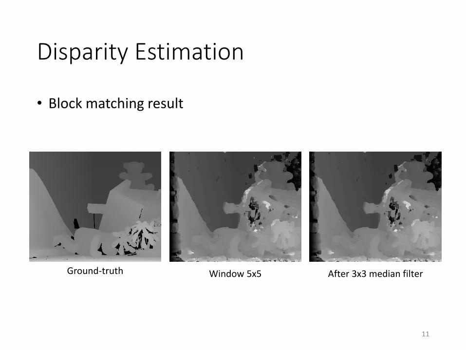
Ground-truth Window 5x5 After 3x3 median filter
• Block matching result

Depth from Disparity
12
baseline 𝑏
𝑃
Visible surface
𝑧
op
tica
l axi
s
op
tica
l axi
s
𝑓 𝑓
𝑥𝐿 𝑥𝑅
• Disparity 𝑑 = 𝑥𝐿 − 𝑥𝑅• It can be derived that
𝑑 =𝑓 ∙ 𝑏
𝑧• Disparity = 0 for distant points• Larger disparity for closer points

Depth Error from Disparity
• From above equation, we can also derive the depth error w.r.t. the disparity error is:
13
𝜖𝑧 =𝑧2
𝑓 ∙ 𝑏𝜖𝑑
Gallup et al. Variable baseline/resolution stereo. In CVPR 2008.

Components of a Stereo Vision System
• Calibrate cameras
• Rectify images
• Compute disparity
• Estimate depth
14

Components of a Stereo Vision System
• Calibrate cameras
• Rectify images
• Compute disparity
• Estimate depth
15
Most stereo matching papers mainly focus on disparity estimation

More on Disparity Estimation
• Typical pipeline
• Matching cost
• Local methods• Adaptive support window weight• Cost-volume filtering
• Global methods• Belief propagation• Dynamic programming• Graph cut
• Better disparity refinement
• More challenges
16

Typical Stereo Pipeline
• Cost computation
• Cost (support) aggregation
• Disparity optimization
• Disparity refinement
17D. Scharstein and R. Szeliski. A taxonomy and evaluation of dense two-frame stereo correspondence algorithms. IJCV 2002.
Block matching algorithm

Matching Cost
• Squared difference (SD):
• Absolute difference (AD):
• Normalized cross-correlation (NCC)
• Zero-mean NCC (ZNCC)
• Hierarchical mutual information (HMI)
• Census cost
• Truncated cost• 𝐶 = min(𝐶0, 𝜏)
18
𝐼𝑝 − 𝐼𝑞2
|𝐼𝑝 − 𝐼𝑞|
Hirschmuller and Scharstein. Evaluation of stereo matching costs on images with radiometric differences. PAMI 2008.
Local binary pattern

Matching Cost
• Deep matching cost (MC-CNN)
19
Zbontar and LeCun. Stereo matching by training a convolutional neural network to compare image patches. Journal of Machine Learning Research. 2016.https://github.com/jzbontar/mc-cnn
Snapshot from Middlebury v3

More on Disparity Estimation
• Typical pipeline
• Matching cost
• Local methods• Adaptive support window weight• Cost-volume filtering
• Global methods• Belief propagation• Dynamic programming• Graph cut
• Better disparity refinement
• More challenges
20

Local Methods
• Cost computation
• Cost (support) aggregation• Adaptive support weight
• Adaptive support shape
• Disparity optimization: winner-take-all
• Disparity refinement
21

Adaptive Support Weight
• Not all pixels are equal• Larger weight for near pixels
• Larger weight for pixels with similar color
22Kuk-Jin Yoon and In-So Kweon. Locally adaptive support-weight approach for visual correspondence search. In CVPR 2005.
It’s bilateral kernel! Computationally expensive

Adaptive Support Shape
• Cross-based cost aggregation
23Zhang et al. Cross-based local stereo matching using orthogonal integral images. CSVT 2009.
Find the largest arm span:

Adaptive Support Shape
• Cross-based cost aggregation
24Zhang et al. Cross-based local stereo matching using orthogonal integral images. CSVT 2009.

Adaptive Support Shape
• Cross-based cost aggregation• Fast algorithm using the orthogonal integral image (OII) technique
25Zhang et al. Cross-based local stereo matching using orthogonal integral images. CSVT 2009.
We only need four additions/subtractions for an anchor pixel to aggregate raw matching costs over any arbitrary shaped regions.

Cost-Volume Filtering
• Illustration of the matching cost
26Rhemann et al. Fast cost-volume filtering for visual correspondence and beyond. In CVPR 2011.
Raw cost
Smoothed by box filter
Smoothed by bilateral filter
Smoothed by guided filter
Ground-truth
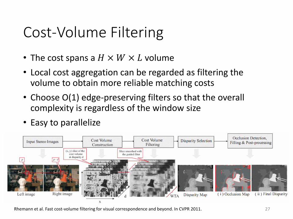
Cost-Volume Filtering
• The cost spans a 𝐻 ×𝑊 × 𝐿 volume
• Local cost aggregation can be regarded as filtering the volume to obtain more reliable matching costs
• Choose O(1) edge-preserving filters so that the overall complexity is regardless of the window size
• Easy to parallelize
27Rhemann et al. Fast cost-volume filtering for visual correspondence and beyond. In CVPR 2011.

Cost-Volume Filtering
28Rhemann et al. Fast cost-volume filtering for visual correspondence and beyond. In CVPR 2011.

Cost-Volume Filtering
• Cost-volume filtering is a general framework and can be applied to other discrete labeling problems• Optical flow: labels are displacements
• Segmentation: labels are foreground/background
29Rhemann et al. Fast cost-volume filtering for visual correspondence and beyond. In CVPR 2011.

Reduce Redundancy
• Two-pass cost aggregation• Pass 1: 5x5 box filter
• Pass 2: adaptive weight filter
30Min et al. A Revisit to Cost Aggregation in Stereo Matching: How Far Can We Reduce Its Computational Redundancy?In ICCV 2011.

More on Disparity Estimation
• Typical pipeline
• Matching cost
• Local methods• Adaptive support window weight• Cost-volume filtering
• Global methods• Belief propagation• Dynamic programming• Graph cut
• Better disparity refinement
• More challenges
31

Global Methods
• A good stereo correspondence• Match quality: each pixel finds a good match in the other image
• Smoothness: disparity usually changes smoothly
• Mathematically, we want to minimize:
• 𝐷𝑝 is the data term, which is the cost of assigning label 𝑑𝑝 to pixel 𝑝.𝐷𝑝 can be the raw cost or the aggregated cost.
• 𝑉 is the smoothness term or discontinuity cost. It measures the cost of assigning labels 𝑑𝑝 and 𝑑𝑞 to two adjacent pixels.
32
𝐸 𝑑 =
𝑝
𝐷(𝑑𝑝) + 𝜆
𝑝,𝑞
𝑉(𝑑𝑝, 𝑑𝑞)
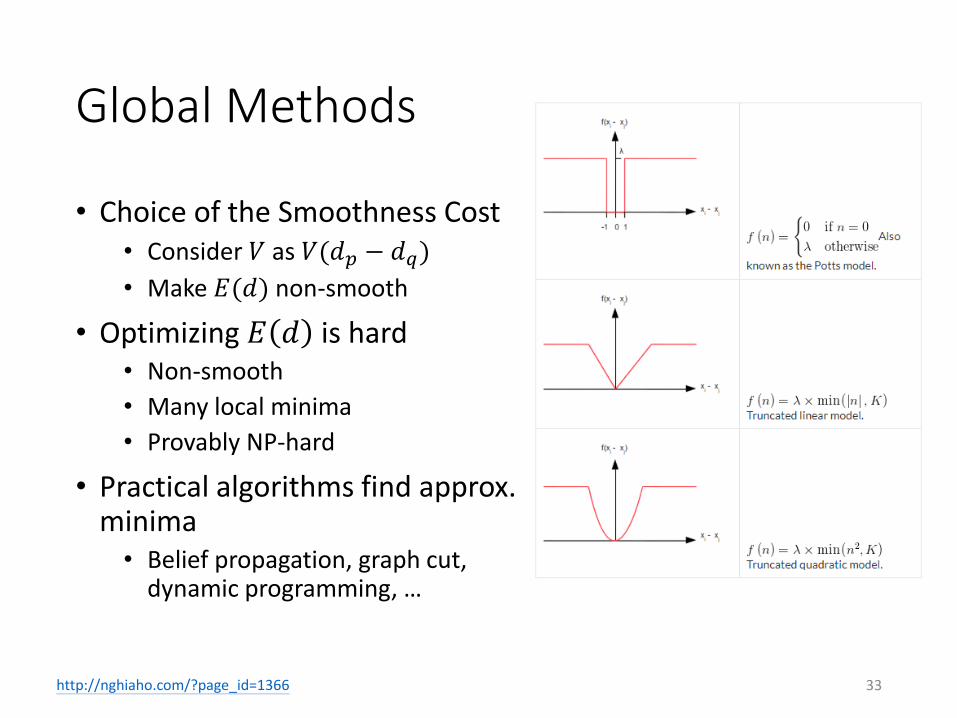
Global Methods
• Choice of the Smoothness Cost• Consider 𝑉 as 𝑉(𝑑𝑝 − 𝑑𝑞)
• Make 𝐸(𝑑) non-smooth
• Optimizing 𝐸 𝑑 is hard• Non-smooth
• Many local minima
• Provably NP-hard
• Practical algorithms find approx.minima• Belief propagation, graph cut,
dynamic programming, …
33http://nghiaho.com/?page_id=1366

Belief Propagation
• BP is a message passing algorithm• Message on each node is a vector sized 𝐿
34http://nghiaho.com/?page_id=1366
Illustration of a 3x3 MRF Message passing to the right
It takes 𝑂(𝐿2) time to compute each message

Belief Propagation
• Loopy BP (LBP): BP applied to graphs that contain loops
35http://nghiaho.com/?page_id=1366
Calculating belief
Overall time complexity is 𝑂(𝐿2𝑇𝑁)

Belief Propagation
• Loopy BP is not guaranteed to converge
• Empirically it converges to good approximate minima.
36http://nghiaho.com/?page_id=1366

Efficient Belief Propagation
• Multiscale BP (coarse-to-fine)
• 𝑂(𝐿) time complexity message passing
37Felzenszwalb and Huttenlocher. Efficient belief propagation for early vision. IJCV 2006.
Rewrite as:
Truncated linear model
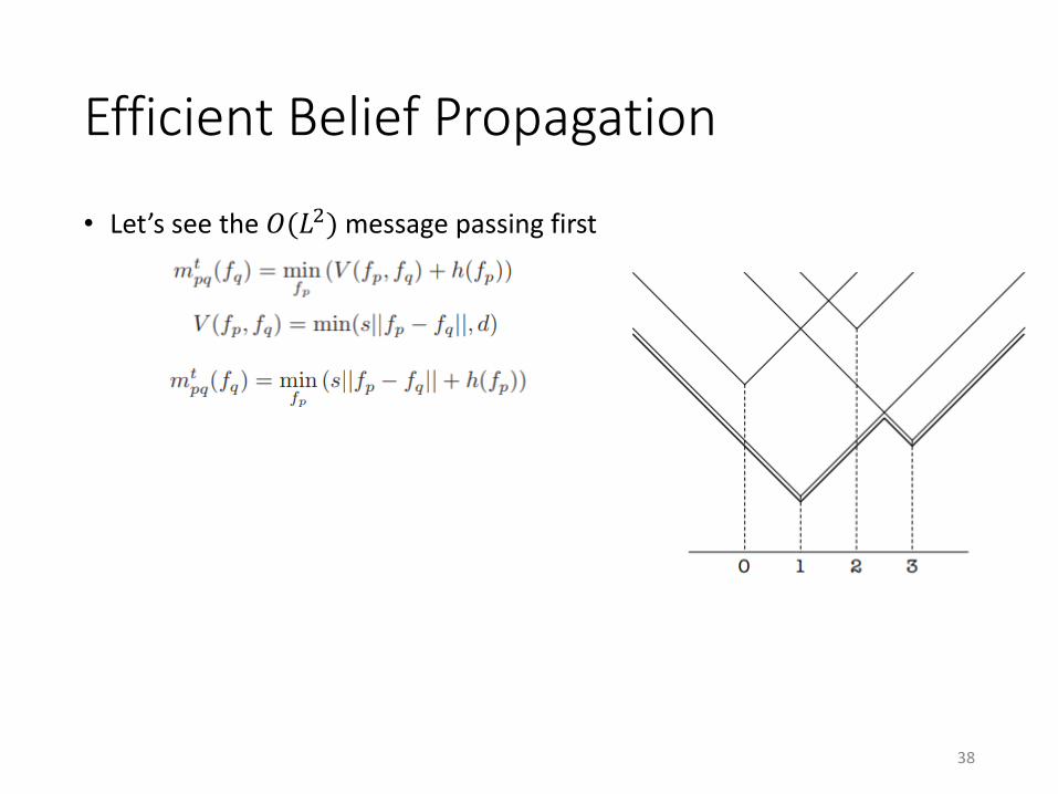
Efficient Belief Propagation
• Let’s see the 𝑂(𝐿2) message passing first
38

Efficient Belief Propagation
• 𝑂(𝐿) time complexity message passing
39Felzenszwalb and Huttenlocher. Efficient belief propagation for early vision. IJCV 2006.
Fast algorithm:

Illustration
40
0 1 2 3
𝑚 = (3,1,4,2)
𝑚 = (3,1,2,2)
𝑚 = (2,1,2,2)
forward pass
Let 𝐿 = 4:
lower envelope
Felzenszwalb and Huttenlocher. Efficient belief propagation for early vision. IJCV 2006.
backward pass

Color Weighted BP
• The message is reliable when 𝑥1 and 𝑥2 have similar color.
41
Yang et al. Stereo matching with color-weighted correlation, hierarchical belief propagation and occlusion handling. In CVPR 2006.
Color weighted smoothness cost:

Belief Propagation
• Other strong variants exists• Double BP
• Constant-space BP
• Hardware-efficient BP
42
Yang et al. Stereo matching with color-weighted correlation, hierarchical belief propagation and occlusion handling. In CVPR 2006.Yang et al. A constant-space belief propagation algorithm for stereo matching. In CVPR 2010.Liang et al. Hardware-efficient belief propagation. In CVPR 2009.
Snapshot from Middlebury v2

Graph Cut
• GC can also be used to minimize
43
𝐸 𝑑 =
𝑝
𝐷(𝑑𝑝) + 𝜆
𝑝,𝑞
𝑉(𝑑𝑝, 𝑑𝑞)
Taniai et al. Graph cut based continuous stereo matching using locally shared labels. In CVPR 2014.Kolmogorov et al. What energy functions can be minimized via graph cuts? PAMI 2004Boykov et al. Fast approximate energy minimization via graph cuts. In ICCV 1999.
Results from Taniai et al.

More on Disparity Estimation
• Typical pipeline
• Matching cost
• Local methods• Adaptive support window weight• Cost-volume filtering
• Global methods• Belief propagation• Dynamic programming• Graph cut
• Better disparity refinement
• More challenges
44

Disparity Refinement
• Left-right consistency check• Compute disparity map 𝐷𝐿 for left image
• Compute disparity map 𝐷𝑅 for right image
• Check if 𝐷𝐿 𝑥, 𝑦 = 𝐷𝑅(𝑥 − 𝐷𝐿 𝑥, 𝑦 , 𝑦)
45
Left view Right view

Disparity Refinement
• Hole filling• 𝐹𝐿, the disparity map filled by closest valid disparity from left
• 𝐹𝑅, the disparity map filled by closest valid disparity from right
• Final filled disparity map 𝐷 = min(𝐹𝐿, 𝐹𝑅) (pixel-wise minimum)
• Why?
46
The above steps do not guarantee coherency between scanlines

Disparity Refinement
• Weighted median filtering
47Ma et al. Constant time weighted median filtering for stereo matching and beyond. In ICCV 2013.Zhang et al. 100+ times faster weighted median filter. In CVPR 2014.

Disparity Refinement
• Weighted median filtering
48Ma et al. Constant time weighted median filtering for stereo matching and beyond. In ICCV 2013.

More on Disparity Estimation
• Typical pipeline
• Matching cost
• Local methods• Adaptive support window weight• Cost-volume filtering
• Global methods• Belief propagation• Dynamic programming• Graph cut
• Better disparity refinement
• More challenges
49
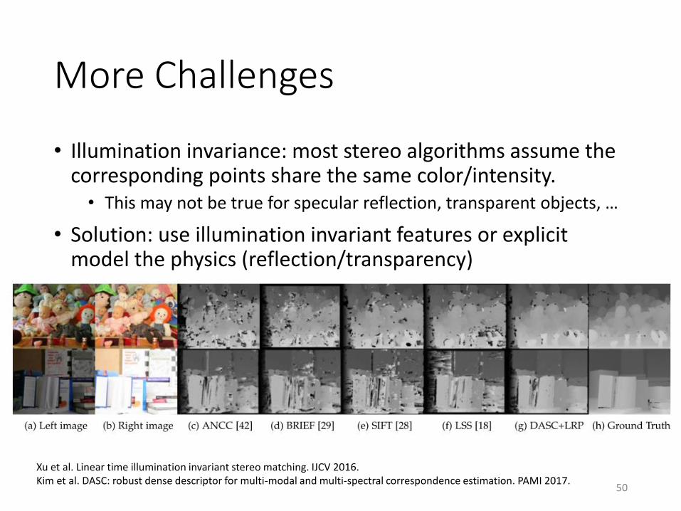
More Challenges
• Illumination invariance: most stereo algorithms assume the corresponding points share the same color/intensity.• This may not be true for specular reflection, transparent objects, …
• Solution: use illumination invariant features or explicit model the physics (reflection/transparency)
50
Xu et al. Linear time illumination invariant stereo matching. IJCV 2016.Kim et al. DASC: robust dense descriptor for multi-modal and multi-spectral correspondence estimation. PAMI 2017.

More Challenges
• Frontal parallel assumption:Cost-volume filtering assumes the world is piecewise flat, so we believe mixing costs for similar pixels can refine the costs.
• In reality, there are many slanted surfaces in the world.
51
A sample view from KITTI 2012 dataset

More Challenges
• Breaking the frontal parallel assumption
52Bleyer et al. PatchMatch stereo – stereo matching with slanted support window. In BMVC 2014.
Local plane fitting:
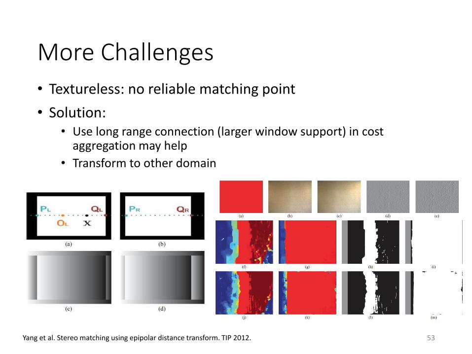
More Challenges
• Textureless: no reliable matching point
• Solution: • Use long range connection (larger window support) in cost
aggregation may help
• Transform to other domain
53Yang et al. Stereo matching using epipolar distance transform. TIP 2012.

Benchmark
• For latest and greatest algorithms, check the following:• Middlebury v3
• Middlebury v2 (still useful but no longer active)
• KITTI 2012
• KITTI 2015
• ETH3D
54

Application: Scene Analysis
• Potential application for visual disability or robots
55Hyun Soo Park, Jyh-Jing Hwang, Yedong Niu, and Jianbo Shi. Egocentric Future Localization. In CVPR 2016.

Application: Synthetic Defocus
• A stereo algorithm tailored for synthetic defocus application
56Barron et al. Fast bilateral-space stereo for synthetic defocus. In CVPR 2015.
Summary
• Depth from disparity
• Standard stereo matching pipeline
• Stereo matching as a • correspondence problem
• labeling problem
• testbed for edge-preserving filtering
• graph optimization problem
• Real world challenges and applications
57