sticky deposit rates - board of governors of the federal ... · pdf fileboard of governors....

Finance and Economics Discussion SeriesDivisions of Research & Statistics and Monetary Affairs

Federal Reserve Board, Washington, D.C.

Sticky Deposit Rates

John C. Driscoll and Ruth A. Judson

2013-80

NOTE: Staff working papers in the Finance and Economics Discussion Series (FEDS) are preliminarymaterials circulated to stimulate discussion and critical comment. The analysis and conclusions set forthare those of the authors and do not indicate concurrence by other members of the research staff or theBoard of Governors. References in publications to the Finance and Economics Discussion Series (other thanacknowledgement) should be cleared with the author(s) to protect the tentative character of these papers.

1

STICKY DEPOSIT RATES JOHN C. DRISCOLL AND RUTH A. JUDSON

FEDERAL RESERVE BOARD1

This Draft: October 1, 2013 ABSTRACT

We examine the dynamics of eleven different deposit rates for a panel of over 2,500 branches of about 900 depository institutions observed weekly over ten years. We replicate previous work showing that rates are downwards-flexible and upwards-sticky, and show that a simple menu cost model can generate this behavior. The degree of asymmetric rigidity varies substantially by deposit type, bank size, and across branches of the same bank. In the absence of such stickiness, depositors would have received as much as $100 billion more in interest per year during periods when market rates were rising. These results also suggest that deposit rates are likely to lag increases in policy and market rates in future tightening cycles.

JEL: E4, G21

Keywords: asymmetric price adjustment, banks, interest rates

1 20th St. and Constitution Ave. NW, Washington DC 20551; Fax (202) 452-2846.

[email protected], (202) 452-2628; [email protected] (202) 736-5612. We thank Anna Thoman and Amanda McLean for outstanding research assistance, and Anna Paulson, Julio Rotemberg, Bill Bassett, and participants at the NBER Monetary Economics and IBEFA conferences for helpful remarks. The views expressed in this paper represent those of the authors, and do not necessarily reflect the views of the Federal Reserve Board or its staff.

mailto:[email protected]

mailto:[email protected]

2

I. Introduction

Retail bank deposits are an important store of value in the United States—totaling over

$6 trillion –and are the sole store of wealth for many U.S. households, particularly less wealthy

ones. According to the 2010 Survey of Consumer Finances (SCF), about two-thirds of

households in the bottom income quintile had bank deposits as assets, while only a single-digit

percentage of such households had any holdings in other liquid financial assets.2 Taken together,

these facts suggest that changes in deposit rates may have economically significant effects on

consumers.

Researchers have long studied the behavior of deposit rates. Hannan and Berger (1991),

Neumark and Sharpe (1992), Diebold and Sharpe (1990), Craig and Dinger (2011), and Yankov

(2012) have shown that rates may take months to change and respond asymmetrically to changes

in banks’ costs of funds (as proxied by the federal funds rate or other interest rates): deposit rates

are upwards-sticky but downwards-flexible. In this paper, we complement this work by using a

high-frequency (weekly) panel dataset observed over a ten-year period for over 2,500 branches

of about 900 depository institutions (DIs) for ten different types of deposit rates.3 Given this

sample, which is both longer and broader than most of those previously used, we are able to

more precisely estimate the duration between interest rate changes and to document the

asymmetry of price adjustment over the course of two full FOMC easing and tightening cycles.

The large number of DI branches allows us to study differences in rate-changing behavior across

institutions; this sort of evidence complements the typical approach in the literature on price-

setting, which looks at changes in the prices of many goods at a single firm or of single goods 2 Holdings of non-bank financial assets, with the exception of the cash value of life insurance, only reach

double digit rates for the third quintile of income and above. See Bricker et al. (2012) for further details.

3 Depository institutions include banks as well as thrifts and credit unions.

3

averaged over many firms. We also document the sluggishness of deposit rate adjustment at the

aggregate level.

We have six key findings. First, some deposit rates are more flexible than others. Rates

on certificates of deposits (CDs) – are quite flexible, with the median institution changing such

rates every 6 to 7 weeks on average. Rates on money market deposit accounts (MMDAs) and

interest checking accounts show much more inertia, changing every 20 weeks and 37 weeks on

average, respectively. By comparison, the target federal funds rate – an important determinant of

DIs’ cost of funds, and thus a good proxy for DI marginal cost – changed about every 12 weeks

across the period. Second, the frequency of rate changes exhibits considerable dispersion for

some types of deposits, with about a quarter of institutions changing interest checking rates twice

a year or less frequently. Third, deposit rate changes are asymmetric: at the institution level,

rates adjust about twice as frequently during periods of falling target federal funds rates as they

do in rising ones. Fourth, rates are uniformly quite sticky during periods when the federal funds

rate is flat, with median durations between price changes ranging from 7 weeks to 37 weeks.

Fifth, the median size of rate changes is 11 to 23 basis points, comparable to the typical 25 basis

point change in the target federal funds rate; the distribution of average decreases and increases

is about the same, and is relatively dispersed, with many small changes of a few basis points.

Sixth, there is a somewhat greater degree of upward stickiness in rates on interest checking and

money market accounts for branches of large DIs than for branches of smaller ones.

We use the results that rates adjust only partially in the weeks and months following an

increase in the target federal funds rate to calculate the costs to consumers of sluggish deposit

rate adjustment. We find those costs to be on the order of about $100 billion per year during

periods when the target federal funds rate rises. With deposit rates near zero as of late 2013,

4

these calculations might be of particular interest as the date of liftoff for the federal funds target

rate approaches.4

We also develop and calibrate a simple menu cost model that, for reasonable parameter

values, can generate the sorts of asymmetric, sluggish adjustment seen in the data.

The rest of the paper proceeds as follows. We provide details on our dataset in section II.

In section III, we document the sluggishness and asymmetry of deposit rate adjustment at the

aggregate level over the past two decades, which includes two episodes of monetary policy

tightening and easing, and we present some rough estimates of dollar value of the gap between

sticky and equilibrium deposit rates. In section IV, we discuss deposit rate behavior at the

microeconomic level. Section V relates our work to previous work on deposit rates. Section VI

presents a simple static menu cost model that yields asymmetric, sluggish price adjustment.

Section VII concludes.

II. Data

The core dataset of this paper is a proprietary weekly micro dataset of bank and thrift

deposit rate data that is collected by Bankrate, Inc.5 This dataset covers several thousand

branches of nearly 900 DIs over a time span of about ten years, from the week of

September 19, 1997 through the week of March 2, 2007. Data for each branch have the parent

institution’s NIC identification code as well as indicators of the banking market. The dataset has

rates on interest-bearing checking accounts, money market deposit accounts (MMDAs), and nine

4 As of September 2013, the FOMC’s most recent Survey of Economic Projections indicated that the

majority of meeting participants expected liftoff to occur in 2015, with projections ranging from 2014 to 2016. http://www.federalreserve.gov/monetarypolicy/files/fomcprojtabl20130918.pdf.

5 http://www.bankrate.com. This dataset is available to users within the Federal Reserve System but, in accordance with the Federal Reserve Board’s contract with Bankrate, Inc., cannot be shared with users outside the Federal Reserve. These data can be purchased directly from the company.

5

different maturities of certificates of deposit (CDs): 3, 6, 12, 24, 30, 36, 48, 60, and 84 months.

The set of branches that provide data is not fully consistent from week to week due to mergers,

exit and entry, and observations of zero, which we believe to be missing observations. The

dataset begins with 443,189 observations, or an average of 897 cross-sectional observations for

each of the 494 weeks in the sample. A relatively small number of observations suffered from

certain irregularities, which we treated as follows.

First, some observations appeared to be partial or full duplicates of others, as if one

observation sometimes contained a partially-completed survey and a separate observation

contained the full set of information. We identified and dropped about 800 such duplicates,

bringing the sample size to 442,407. Second, some observations also were incomplete but were

followed by one or more additional observations with the same bank identification number and

market rank and complementary data. Combining these observations eliminated about 22,000

observations and brought the sample size to 419,881 observations. Finally, we deleted the 55

observations that contained data for only one week, leaving us with 419,826 observations. The

remaining dataset contained information on rates of 2,770 branches for 897 DIs.

A. Comparison with other data sources

One other source of interest rate data at the bank level has been used in previous work.

Hannan and Berger (1991) and Neumark and Sharpe (1992) used the Federal Reserve’s Monthly

Survey of Selected Deposits and Other Accounts (also known as the FR 2042; hereafter the

Monthly Survey). The survey collected the most commonly offered rate by account type;

starting in 1989, the surveys allowed for the possibility that higher rates were offered for larger

balances, a policy known as tiering. The Monthly Survey stopped collecting information on

offered interest rates in 1994 and was discontinued in 1997.

6

An additional potential source of deposit rate data is the quarterly Consolidated Reports

on Condition and Income, known more generally as the Call Reports. These quarterly financial

statements, available since 1934, do not provide direct measures of deposit rates for commercial

banks.6 However, one can divide the interest expenses paid by the bank by the quantity of

deposits in the account to obtain a weighted average of interest rates paid. A disadvantage is

that, in the case of time deposits, the rate may not reflect current offered rates. Another

disadvantage is that some categories of deposits are combined.7

An advantage of using the Bankrate data over the Monthly Survey is that the longer time

series allows us to more accurately estimate longer durations of price stickiness. Moreover, the

weekly frequency of the data allows us to see changes at a higher frequency than either the

Monthly Survey or the Call Reports. A further advantage is that this data is collected for a wider

variety of deposit types than other sources: we observe data on interest checking accounts,

MMDAs, and CDs with nine different maturities. Finally, the Bankrate data is collected for a

much larger group of DIs than the monthly survey, and at the branch level, allowing for better

cross-sectional comparisons.

A significant disadvantage of the Bankrate data is that it appears to reflect only the

lowest rate offered by deposit type. Rice and Ors (2006) document that the Bankrate data, on

average, has significantly lower rates than the quarterly call report-based measures, suggesting

that a substantial fraction of deposits are paid at higher rates.

6 The comparable reports for savings and loans (thrifts) do provide direct measures of offered deposit

rates. 7 In part to avoid having deposit liabilities that are subject to reserve requirements, over the period

analyzed, some banks “sweep” balances from reservable liabilities to non-reservable ones overnight, restoring them the following morning. This sweeping makes measurements of particular account types difficult. The Call Reports deal with this problem by aggregating reservable and non-reservable types of accounts.

7

The discrepancy in the average level of rates among datasets may not be completely

problematic for our purposes. First, it is not clear that the stickiness properties of the rates on the

bottom tier are different from those on upper tiers. As we show below, rates are sticky both at

the aggregate level and the microeconomic level, suggesting that the Bankrate data is capturing

the degree of price inflexibility appropriately. Second, although most deposits are likely paid at

higher tiers, it is not clear that most depositors are receiving such rates, since the distribution of

holdings across consumers is not uniform. To establish the importance of tiering, we surveyed

10 large banks and thrifts and 10 small banks and thrifts listed at the Bankrate website, which has

more information on deposit rates by tier, to find average tiering levels. We found that the

median levels at which tiering starts was $5,000 for MMDAs and interest checking accounts and

$10,000 for CDs. Next, we used data from the 2004 Survey of Consumer Finances (SCF) to

determine what fractions of households who hold those types of deposits have holdings below

the tiering level. We find that about 76 percent of households with interest checking accounts

have balances below the first tier cutoff of $5,000; for savings accounts and CDs, the analogous

figures are 60 percent and 36 percent respectively. We conclude that the Bankrate interest rates

are economically meaningful to a large number of households.8

III. Behavior of Aggregate Deposit Rate Data

A. Overview

We begin by showing that stickiness of deposit rate data is apparent even at the aggregate

level. Figure 1 illustrates the slow asymmetric adjustment of aggregate deposit rates to market

rates. The figure plots the time series of the overall return to M2, the heavy gray line, and

8 Ratewatch.com, and additional source of banking data, including deposit and loan rates and fees,

provides rate data at various tiers. The sample period is shorter than that for the Bankrate.com data.

8

returns to small time deposits and liquid deposits, the gray dashed lines, along with the federal

funds target rate and the three-month Treasury bill rate, the blue and black lines, respectively.9

Notably, over 2001, the federal funds target declined precipitously, while deposit rates initially

declined more slowly than the target rate but then began to keep pace with the declines in the

target rate. As the target rate rose beginning in late 2004, deposit rates rose much more slowly.

To better highlight the asymmetry of deposit rate adjustment, Figure 2 breaks up Figure 1

into periods during which the federal funds rate is falling or flat (upper panel), rising or flat

(lower panel). The upper panel shows that deposit rates fall by closer to the same amount as the

target federal funds rate, and the declines begin sooner after the initial decline in the federal

funds rate. The lower panel shows that the M2 own rate, liquid deposit rate, and small-time

deposit rate increases by much less than the corresponding increases in the federal funds rate;

moreover, the M2 own rate continues to be flat or decline even after increases in the federal

funds rate have begun. In the next subsection, we document this asymmetric sluggishness more

formally by estimating some simple models.

B. Evidence of Sticky and Asymmetric Adjustment in Aggregate Data

We model the time-series behavior of aggregate deposit rates as depending on their own

lagged values and on market interest rates. We estimate the regressions below over a sample that

begins in July, 2000, the beginning of the most recent full easing cycle, and ends in July 2007,

just before the recent financial turmoil began.

9 The overall M2 rate, or “own rate,” is calculated as the deposit-weighted average of rates paid on the

major components of M2, which are liquid deposits, small time deposits, currency (zero), and retail money market mutual funds. The small time deposit rate is proxied by the six-month CD rate provided by Bankrate. “Liquid deposits” is the sum of checking and savings deposits, including MMDAs; this summation is done in order to control for the effects of sweeping, described in footnote 7 above. The liquid deposit rate is constructed based on Call Report and Bankrate data. Rates on money market mutual funds are provided by ICI.

9

Tables 1 and 2 present results for of the change in two aggregate Bankrate deposit rates,

the MMDA rate and the six-month CD rate. These aggregate rates are constructed by Bankrate

as the simple average of the rates offered by the top five banks in each of the top ten banking

markets. The movements in these rates are regressed on their own lags and on the federal funds

rate target and the three-month T-bill rate, with separate slope coefficients for periods when the

federal funds rate target is rising or steady and for when it is falling. The three-month Treasury

bill rate is commonly used in the computation of the opportunity cost of holding money, as it

represents the rate on an asset that may be a close substitute to money and thus affects the

demand for deposits. The target federal funds rate, which is highly correlated with the T-bill rate,

is related to the marginal cost to the DI of an extra dollar of deposits, and thus influences the

supply of deposits.10 11 Both of these rates move essentially continuously and can be easily

observed at a daily frequency.

In Table 1, the dependent variable is the change in the deposit rate (the commercial bank

MMDA rate or six-month CD rate) and the independent variables are the lagged deposit rate, the

change in the effective federal funds rate, and the change in the federal funds rate interacted with

a dummy variable that is one when the change is positive or zero and zero otherwise.12 A

significant t-statistic on this last variable indicates that the response is asymmetric, or

significantly different, when the rate is rising relative to the baseline of steady or falling rates.

10 On deposits subject to reserve requirements, the federal funds rate is the cost to the DI of borrowing to

fulfill the requirement (or the opportunity cost of holding reserves for DIs who do not need to borrow). Over this sample, the daily effective federal funds rate was, on average, within two basis points of the target and was seldom more than five basis points away from the target.

11 One might consider the LIBOR or repo rate as well, but over the period in question, these rates are essentially identical to the effective federal funds rate.

12 All t-statistics are computed using standard errors that are robust to heteroskedasticity and serial correlation in the errors.

10

The overall pace of deposit rate adjustment when market rates are rising can be calculated as the

sum of the two coefficients on the market rates.

Table 1: Weekly Changes in Deposit Rates and FFR

BRM-CB MMDA Rate BRM-6-Month CD Rate

Full Early Late Full Early Late

Commercial bank MMDA rate, lag -0.001+ -0.001 -0.004*

(-1.7) (-0.1) (-2.5)

Fed funds target change 0.100* 0.111* 0.094* 0.384* 0.391* 0.371*

-10 -2.5 -9.3 -18.9 -6.1 -16.2

Fed funds target rise -0.055* -0.043 -0.067* -0.286* -0.282* -0.283*

(-3.3) (-0.9) (-3.5) (-8.3) (-3.9) (-6.5)

Commercial bank 6M CD rate, lag

-0.001 0.004 -0.004*

(-1.1) -0.9 (-3.4)

Constant -0.001 -0.002 0.001 0.003 -0.016 0.009*

(-0.6) (-0.2) -0.7 -1.1 (-0.7) -2.6

Observations 551 181 370 551 181 370 R2 0.18 0.08 0.24 0.41 0.23 0.45 Adjusted R2 0.18 0.07 0.24 0.41 0.22 0.45

t statistics in parentheses + p<0.10, * p<0.05

For both deposit rate measurements, weekly adjustment to changes in the federal funds

rate is far below unity, ranging from 10 basis points per percentage point of change for liquid

deposit rates to 39 basis points per percentage point of change in the effective federal funds rate

for small time deposits during times of stable or falling rates. Moreover, this stickiness is even

stronger when the federal funds target is rising: for MMDA rates, the coefficient drops

considerably, to 3 to 7 basis points per percentage point of change in the federal funds rate target;

for the six-month CD rate, the coefficient drops to around 10 basis points per percentage point

change in the federal funds rate target. Results are similar for the three-month bill rate, shown in

11

Table 2. Indeed, the regression results indicate that upward adjustments to savings rates are

approximately zero at a weekly frequency when the federal funds target is rising.

Table 2: Weekly Changes in Deposit Rates and T-Bill rate

BRM-CB MMDA Rate BRM-6-Month CD Rate

Full Early Late Full Early Late

Commercial bank MMDA rate, lag -0.002* -0.003 -0.006*

(-2.1) (-0.8) (-3.6)

3-month T-bill rate change 0.082* 0.011 0.083* 0.479* 0.205* 0.499*

-5.9 -0.3 -5.6 -17.3 -3.1 -16.2

3-month T-bill rate change, FFR rising -0.083* -0.021 -0.083* -0.390* -0.177* -0.363*

(-4.8) (-0.4) (-4.2) (-11.4) (-2.5) (-8.7)

Commercial bank 6M CD rate, lag

-0.001 0.009+ -0.004*

(-0.6) -1.7 (-3.1)

Constant 0.000 0.004 0.002 0.001 -0.039 0.007+

(-0.2) -0.5 -1.5 -0.4 (-1.6) -2.0

Observations 551 181 370 551 181 370 R2 0.07 0.01 0.13 0.37 0.07 0.47 Adjusted R2 0.06 -0.01 0.13 0.37 0.06 0.46

t statistics in parentheses + p<0.10, * p<0.05

Much as slow adjustment of prices does not necessarily represent a cost to consumer

because prices that are slow to rise can be advantageous to consumers, sticky deposit rates are

not necessarily disadvantageous to consumers. Indeed, in the years of the financial crisis, a

period beyond the sample examined in this period, deposit rates fell much more slowly than

market rates, presumably benefiting depositors.13 Nonetheless, when rates are slow to rise, the

13 Indeed, the standard models of demand for M2 faced a considerable challenge in this period. The

standard formulation of demand for M2 posits a relationship between the ratio of income to M2 and opportunity cost, or the difference between an alternative rate and the rate paid on M2. This rate is assumed to be positive, and yet it dropped well below zero as rates of adjustment on deposits lagged well behind the precipitous drops in market rates seen in late 2008 (see Judson, Schlusche, and Wong (2012 mimeo).

12

reductions in interest income to consumers can be considerable. Moreover, if the stickiness is

asymmetric, as we show that it is for deposit rates, it is possible that the differences between

actual and “equilibrium” or “nonsticky” rates could be costly to consumers on net.

Over the period examined here, we attempt a rough calculation as follows. First,

following Moore, Porter, and Small (1989), we identify an equilibrium rate relationship by

identifying periods of relatively stable deposit rates. These periods coincide (not surprisingly)

with periods when the federal funds rate target had been stable for at least three months. We

then estimate a least squares regression using these “equilibrium” observations and apply the

coefficients to the whole sample. We then calculate the average difference between the actual

and “equilibrium” rates. This rough calculation indicates that, over the sample period, actual

deposit rates were about 15 to 25 basis points below actual rates. At current quantities of

deposits, this difference would amount to an interest loss of about $15 billion (20 basis points x

$7 trillion in savings in small time). These losses, however, are concentrated in times when rates

are rising.

Looking forward, when interest rates lift off from their current levels near zero, these

results suggest that deposit rates are likely to follow very slowly. Over the sample in this paper,

the maximum gap between actual and “equilibrium” deposit rates was between 100 and 160

basis points; such a gap would represent a loss to consumers of about $70 billion to $100 billion

per year. In the next section, we use the micro-level information to calculate the speed with

which deposit rates are likely to rise when the target federal funds rate begins to lift off from its

current near-zero level.

13

IV. Deposit Rate Behavior at Individual Branches

A. Durations between Rate Changes

1. Results

The results of the previous section show that at the aggregate level, deposit rates are

sluggish and adjust symmetrically. In this section, we look at the adjustment of deposit rates at

the depository institution (DI) branch level. Figure 3 plots histograms, by deposit type, of the

average number of weeks between interest rate changes. For each DI branch, we compute the

average by dividing the number of weeks the DI branch is in the sample by the number of

interest rate changes observed. The first row displays histograms for 6-month and 24-month

certificates of deposit (CDs) respectively.14 The second row presents histograms for money

market deposit accounts (MMDAs) and interest checking accounts, respectively. Insets in each

chart give the medians of the average number of weeks between rate changes.

The charts in the first row show that CD rates change relatively quickly: the median

number of weeks on average between rate changes ranges from 6.0 to 7.0, implying that rates

change every month or two. The distribution across banks is fairly tight, and few banks average

more than 15 weeks between changes for CD rates.

By contrast, the second rows shows considerably longer durations between interest rate

changes for MMDAs (left panel) and interest-bearing checking accounts (right panel). The

median average duration between price changes is about 20 weeks – or five months – for

MMDAs and about 37 weeks—or about 9 months – for interest checking accounts. Moreover,

there is much greater diversity in behavior across DI branches with these accounts than for CDs:

over a quarter of DI branches change MMDA rates on average about every 8 months or less 14 Maturities charted are 6 and 24 months. Data for 30-, 48-, and 84-month maturities are available in

the dataset but are relatively sparse. Data for 3-, 12-, 36-, and 60-month maturities are similar and are available in an online appendix.

14

frequently, while about the same percentage of DI branches change interest checking rates on

average yearly or less frequently.

2. Measuring the Degree of Deposit Rate Stickiness

As we noted above in our discussion of aggregate deposit rates, we would expect rates to

move in response to changes in deposit demand and supply; thus, rates would be fully flexible if

they changed at least as frequently as measured demand or supply shocks. Standard models of

money demand suggest that deposit demand should depend on deposit opportunity cost, the

difference between a short-term interest rate and the deposit rate. Since the 3-month T-bill rate,

like other deposit rates, changes nearly continuously, fully flexible deposit rates should also

adjust, at least to some extent, continuously.15 Arguably, then, all deposit rates across all DI

branches are sticky, since no DI branch on average changes any of its deposit rates at a weekly

frequency.

It is possible that deposit demand itself responds sluggishly to changes in opportunity

cost. Thus, the response of deposit rates to shocks to deposit supply may be a more accurate

guide to how sticky deposit rates are. As noted above, the effective federal funds rate represents

the marginal cost of an additional dollar of many kinds of transactions deposits. Moreover, bank

prime lending rates, which in turn determine the pricing for many loans, are typically set as a

fixed margin over the target federal funds rate. Hence the federal funds rate is an important

determinant of both marginal cost and marginal revenue.

Over the 494 weeks of the sample period, the FOMC changed its target federal funds

rate 39 times, implying an average time between changes of 12.6 weeks. By this standard, CD 15 Deposit rates need not adjust by the full amount of the shock; doing so would complete undo the

demand shock. However, if there is no adjustment in deposit rates—as appears to be the case here—then the adjustment is purely in quantities, suggesting a horizontal supply curve and thus completely sticky deposit rates.

15

rates are quite flexible, changing almost twice as frequently as the target federal funds rate;

median MMDA rates change somewhat less often than the federal funds rate, though there is a

long tail of DIs that change rates much less frequently; and interest checking rates are relatively

sticky.

If we took as a criterion for having sticky deposit rates that a DI branch changed rates

less frequently than the change in the target federal funds rate, then between about 5 to 20

percent of DI branches have sticky CD rates; about 75 percent have sticky MMDA rates; and

over 90 have sticky interest checking rates.

Deposit rates are generally somewhat more flexible than goods prices; Klenow and

Kryvstov (2008) and Nakamura and Steinsson (2006a) found that posted goods prices on average

change about every four months; depending on how one accounts for sales, this figure can rise to

eight months. However, deposit rates change much less frequently than the prices of many other

financial assets that are alternative stores of value, such as equities or bonds (on the secondary

market), which may change minute to minute.

3. Asymmetric Response of Deposit Rates to the Federal Funds Rate

From our results with the aggregate data, we suspect that there will likely be an

asymmetric response of deposit rates to changes in the target federal funds rate, with faster

responses to increases in the target than to decreases. We explore this hypothesis in Figure 4.,

where we break up the sample into time periods during which the federal funds rate is rising (left

column), time periods during which it is falling (middle column), and periods during which it is

flat (right column). The left and middle columns show histograms of the average number of

weeks between rate changes during periods of falling and rising target federal funds rates

respectively. It is immediately apparent that rates are much more flexible during periods of

16

falling target rates. For CD rates, the median number of weeks between price changes ranges

between 3 and 4 weeks during periods of falling target rates but around 74 weeks during periods

of rising rates. In addition, the distributions are much more compressed during periods of falling

rates. The same general pattern holds true for MMDAs and interest checking, though the

distributions during periods of rising funds rate have much wider supports, with the average

number of weeks between price changes exceeding two years for some DIs.

The right-hand column of Figure 4 shows the same data during periods where the target

federal funds rate is flat. The rates generally show much greater median intervals between rate

changes: for CDs, medians range between 7 and 9 weeks; for MMDAs, the median is 24 weeks,

and for interest checking, 37 weeks. Moreover, the distributions in average rate changes across

DI branches are wider, particularly in the cases of CD rates. Given the absence of a clearly

important shock to deposit supply—federal funds rate changes—it is perhaps not surprising that

durations between rate changes rise, although the high value of the median suggests that other

shocks to deposit demand and supply may not be quantitatively important determinants of

deposit rates. However, it is not clear to us why the dispersion in the distribution of average

weeks between rate changes should rise.

4. Dynamic Response of Deposit Rates to Target Federal Funds Rate Changes

The results above show relatively sluggish responses of many deposit rates to changes in

the target federal funds rate. In Figure 5, we further explore the dynamic path of responses to

target rate increases and decreases. Each panel on the first page of figure 4 reports the

cumulative fraction of DI branches to have made any change in its deposit rate following the 25

17

basis point increase in the target federal funds rate at the June 1999 FOMC meeting.16 We plot

the fractions for 26 weeks following the FOMC meeting; it is worth noting that another rate

increase occurred at the next meeting, 7 weeks later. The charts show that only a very small

fraction of DI branches make any change in their deposit rates in the week following the

meeting—nearly zero in the case of interest checking and MMDAs, to about 20 percent for

longer-maturity CD rates. For CD rates with maturities of more than 6 months, the fractions rise

by nearly 10 percent per week, so that by the time of the next FOMC meeting, between 50 and

70 percent of DIs have adjusted their deposit rates. In contrast, MMDA and interest checking

rates are extremely sluggish to change; by the time of the next FOMC meeting, only 10 to 20

percent of DIs have adjusted their rates.

The second page of Figure 8 shows comparable results for the January 2001 intermeeting

decrease in the federal funds rate; in this case, the next decline occurred four weeks after the first

decline.17 A somewhat larger fraction of DI branches changed their CD rates immediately than

in the case of the increase in the target rate. After four weeks, the vast majority of branches had

changed their longer-maturity CD rates. Again in contrast, only a small fraction of branches

changed their MMDA or interest checking rates in the weeks following the change.

Taken together, the results confirm that DI branches respond both sluggishly and

asymmetrically to changes in the target federal funds rate. Moreover, the average fractions of

price changes each week are quite low—even among the deposit rates for which branches are

comparably more responsive to changes in the target federal funds rate, only about 10 percent

per week of DI branches are changing rates. 16 We choose that meeting because it was at the beginning of a tightening cycle; thus, deposit rates were

not still responding to previous changes in the target federal funds rate. 17 An additional feature of this change in the target rate was that it was likely more unexpected than other

changes, since it did not occur during a regularly scheduled meeting.

18

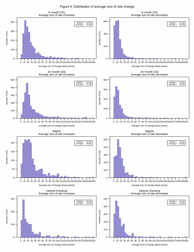
5. Size of Deposit Rate Changes

We next look at the average size of rate increases and decreases. As in menu cost

models, if infrequent deposit rate changes are caused by costs of changing rates, we should see

relatively large rate changes. Figure 6 plots histograms of the size of rate increases (left-hand

charts) and rate decreases (right-hand charts) by deposit types. As with prices of other goods, we

see a fairly wide range of price changes, including some small changes. Median changes are in

the 10 to 20 basis point range, comparable to the typical 25-basis-point sized change in the

federal funds rate. The distributions of size by increases and decreases do not seem to differ in

economically significant ways.

6. Differences by DI size

Finally, we look at the distribution of branch-level deposit rate changes by size of the

parent DI, since larger institutions may act differently towards their customers than smaller ones.

Figure 7 displays the same calculations as Figures 3 and 4, but for branches belonging to the top

ten banks (by total deposits) in each time period.18 A comparison of Figure 3 to Figure 7 shows

that CD rates at large banks behave similarly to all banks: median durations between rate

changes differ by a week or less. MMDA and interest checking rates appear to be somewhat

more sluggish at larger banks. The median duration between rate changes for MMDA rates was

22.7 weeks at large banks and 20 weeks at all DIs; the figures for interest checking are 41.1 and

37.0 weeks, respectively. There also appears to be considerably more dispersion in the duration

of interest rate changes at larger banks.

A comparison of Figures 4 and 7 shows that the difference in the number of weeks

between rate changes across periods of rising and falling federal funds rates is greater for 18 At the end of 2007, Call Report data showed that these institutions held about 30 percent of all interest

checking deposits, half of all savings deposits, and 34 percent of all small time deposits.

19

branches of large DIs than for branches of all DIs. For example, the differences in median

durations for MMDA rates across rising and falling periods are both about 13.7 and 23.7,

compared with 12.7 and 20.8 weeks, respectively, for all DIs. On the whole, larger banks raise

deposit rates more sluggishly during periods of rising federal funds rates.

Table 3: Median of average number of weeks between rate changes

Branches of top 10 Branches of top 10 Full

sample Fed

funds rate

falling

Fed funds target rising

Fed funds target

flat

Full sample

Fed funds rate

falling

Fed funds target rising

Fed funds target

flat 6-month CD 7.0 3.8 6.8 9.8 7.1 3.5 6.7 8.6

24-month CD 6.0 3.4 7.4 7.3 5.5 2.9 8.0 6.0 MMDA 20.0 12.7 20.8 24.0 22.7 13.7 23.7 30.5

Interest checking 37.0 22.2 50.3 37.4 41.1 25.8 104.0 45.7

In contrast, a comparison of Figures 4 and 7 shows relatively little qualitative difference

in average durations of rate changes between branches of larger DIs and branches of all DIs

during periods where the federal funds rate is flat for CDs, though adjustment is more sluggish

for MMDA and interest checking rates. A comparison of Figures 5 and 8 similarly shows

relatively little difference in the distribution of the size of interest rate changes between large

banks and all DIs.

Taken together with the above results for the rising and falling periods, it seems that

larger DIs respond more strongly to changes in the federal funds rate than smaller DIs, but do not

react in a different way to other deposit demand and supply shocks.

One other notable feature of these figures is that they contain far more than ten

observations, since large DIs tend to have many branches. The still-considerable dispersion in

the average duration of rate changes across DI branches thus indicates that deposit rate setting

20

behavior varies across branches of the same institution. One might have thought a priori that

there would be standard policies for each DI, and that we would therefore see clustering in the

histograms around ten or fewer points.

Finally, these findings are broadly consistent with the aggregate regression results

reported above: first, deposit rates are sticky, or adjust at a less than one-for-one pace to

movements in market rates; second, the adjustment is asymmetric: coefficients of adjustment are

significantly lower when the federal funds target and market rates are rising than when such rates

are falling; third, rates are stickier for savings deposits than for time deposits.19

V. Relation to Previous Work on Deposit Rates

Several earlier papers have documented stickiness and asymmetric behavior in deposit

rates. Hannan and Berger (1991) look at monthly observations on money market deposit

accounts (MMDAs) of 398 banks from September 1983 to December 1986 from the Federal

Reserve’s Monthly Survey of Selected Deposits and Other Accounts. Hannan and Berger find

that, of the 12,179 observations, 2,471 involved rate increases, 5,338 decreases, and 4,370 no

rate change. They estimate multinomial logit models of the decision to change deposit rates,

finding that banks have a 62 percent probability of reducing deposit rates in response to a

decrease in the 3-month Treasury bill rate of 29 basis points (the mean absolute change over their

sample), but only a 39 percent probability of raising rates in response to an equal-sized increase.

They further show that banks in more concentrated markets have more rigid prices; larger banks

have more flexible prices; and banks with larger market customer bases have less rigid prices.

19 Results are similar when these regressions are estimated on aggregate M2, liquid deposit, and small

time rates, which are deposit-weighted rather than simple averages and which cover virtually all deposits rather than only commercial bank MMDA and CD deposits.

21

Neumark and Sharpe (1992) look at the same survey, using monthly data on six-month

certificates of deposits (CDs) and MMDAs for 255 banks from October 1983 through November

1987. They estimate a partial adjustment model, in which the long run deposit rates are assumed

to be proportional to the six-month Treasury bill rate. The speed of adjustment is allowed to

depend on concentration ratios and other market characteristics. They find that MMDA rates

appear to adjust more sluggishly than CD rates. When rates are constrained to adjust

symmetrically, concentration ratios appear to affect the long-run level of the markup of deposit

rates over Treasury bill rates, but have little impact on the speed of adjustment. They estimate

switching models to test for asymmetry in deposit rate setting. They find that rates adjust more

slowly upwards than downwards, with banks in more concentrated markets being slower to

adjust deposit rates upwards and faster to adjust deposit rates downwards. The long-run

equilibrium markup is lower when asymmetry is allowed for.

Diebold and Sharpe (1990) examine the dynamic relationships among retail (deposit)

rates and wholesale (federal funds and Treasury bill) rates. For deposit rates, they use weekly

data on 6-month CDs, MMDAs, and super NOW (interest checking) accounts from Bank Rate

Monitor (the predecessor of Bankrate, Inc.) from October 5, 1983 to December 25, 1985. The

rates are averaged over 25 major banks and 25 major thrift institutions. They find that wholesale

rates generally Granger-cause retail rates, but the latter do not Granger-cause the former. Retail

rates have hump-shaped and persistent responses to innovations in wholesale rates. It takes

about 2 weeks for one quarter of the response of retail rates to a shock to wholesale rates to

manifest itself; about 5 weeks for half of the response, and about 10 weeks for three quarters of

the response.

22

These four papers were written shortly after deposit rates were deregulated in the 1980s

and were thus based on relatively short samples, making it difficult to precisely estimate the

frequency of deposit rate adjustment. Moreover, during these earlier sample periods, changes in

the target federal funds rate were not publicly announced, making it more difficult to evaluate the

response of deposit rates to changes in this variable.

Craig and Dinger (2011) use Bankrate data, as we do, over about a ten-year period to

document asymmetric stickiness in both deposit rates and in consumer loan rates. They estimate

that the hazard rate of a change in deposit rate increases is hump-shaped with time, increasing for

about the first six weeks before decreasing thereafter. They find that deposit-rate changes are

also state-dependent, and that the hazards of changing deposit rates depend importantly on

market share. Their paper uses a somewhat smaller sample than ours (624 branches as opposed

to 2,500), and thus does not focus on differences in behavior across branches of the same

institution. We also present results on the size of deposit-rate changes, on the aggregate behavior

of deposit rates, and a simple model explaining aggregate stickiness.

Rosen (2002) develops a model with heterogeneous consumers (some of whom respond

to lagged information) to explain asymmetries in deposit-rate stickiness (or indeed other kinds of

price stickiness). He shows that the model is consistent with the behavior of deposit rates in a

smaller set of data from Bankrate.

Yankov (2012) examines the behavior of CD rates over the most recent 15 years, 1997-

2011, using data from RateWatch. He finds that dispersion of yields across institutions indicates

monopoly power that is consistent with an asset-pricing model with varied search costs across

consumers. Yankov’s cross-section and time series are larger than in our paper, though his focus

is on one particular type of deposit rate. His model takes an asset-pricing approach, in which

23

demand for deposits is not related to the monetary services which they provide. His data source

also does not have differences across bank branch.

VI. Modeling Asymmetric Deposit Rate Adjustment

The asymmetric sluggishness of deposit rates documented above is uncharacteristic of the

behavior of prices of other kinds of financial assets. Equity prices vary tick-by-tick, and though

yields on many, but not all, kinds of debt are constant until maturity, secondary-market yields

and prices of debt also move continuously. However, prices of individual goods and services do

show the same sort of asymmetric stickiness that deposit rates do. In this section, we first

document other attempts to model deposit rates and goods prices. We then present a simple,

static menu cost model of deposit rate setting, adapted from the literature on goods and service

prices. We calibrate the model and show that, for reasonable parameter values, it can generate

asymmetric, sluggish adjustment in deposit rates comparable to that seen in the data.20

A. A Simple Model of Asymmetric Deposit Rate Adjustment

In this section, we present a standard static menu-cost model of a bank that generates an

asymmetric range of inaction in deposit rates around the optimum. There are N banks, indexed

by i. Let 𝐷𝑡𝑖 denote deposits held at bank i at time t, 𝑟𝑡𝐷,𝑖 the interest rate paid on those deposits,

and 𝑟𝑡𝐷 the average deposit interest rate (so 𝑟𝑡𝐷 = 1𝑁∑ 𝑟𝑡

𝐷,𝑖) Suppose demand for deposits at bank i

is given by:

𝐷𝑡𝑖 = 𝜙𝐷�1 + 𝑟𝑡𝐷 − 𝑟𝑡𝐷,𝑖�

−𝜂(𝜙𝑂𝐶(1 + 𝑂𝐶𝑡))−𝜓

where 𝑂𝐶𝑡 = 𝑟𝑡𝑠 − 𝑟𝑡𝐷is the opportunity cost of holding deposits, defined as the difference

20 The model is monopolistically competitive, and thus also shows that the pattern of asymmetric

stickiness does not require any collusive behavior among depository institutions.

24

between a short-term interest rate 𝑟𝑡𝑠 and the average interest rate on deposits 𝑟𝑡𝐷, η > 1, and

Ψ > 1. The first term in the demand function captures the degree to which bank i gains(loses)

market share if its deposit rate is greater(less) than the average. The second term is a standard

money demand function, in which demand for overall deposit holdings depends negatively on

the opportunity cost of holding deposits relative to a short-term interest rate. Suppose that that

rate is a constant markup 𝜇𝑆 over a market interest rate 𝑟𝑡𝑀 such as the federal funds rate, so that

𝑟𝑡𝑠 = 𝜇𝑆 + 𝑟𝑡𝑀.

Suppose a bank’s profit per unit of deposit—i.e. its net interest margin—is given by:

𝑟𝑡𝐿,𝑖 − 𝑟𝑡

𝐷,𝑖, where 𝑟𝑡𝐿,𝑖is the interest rate on loans (for simplicity, we ignore securities and other

bank assets). Further suppose that loan rates are equal across banks and are a constant markup

𝜇𝐿 over the market rate, so that 𝑟𝑡𝐿 = 𝜇𝐿 + 𝑟𝑡𝑀. In practice, many loans are priced off of the

prime rate, which is usually a 300 basis point markup over the target federal funds rate. Total

bank profits are then given by:

Π𝑡 = �𝜇𝐿 + 𝑟𝑡𝑀 − 𝑟𝑡𝐷,𝑖�𝜙𝐷�1 + 𝑟𝑡𝐷 − 𝑟𝑡

𝐷,𝑖�−𝜂

(𝜙𝑂𝐶(1 + 𝑂𝐶𝑡))−𝜓

Profit maximization (assuming the bank ignores its small effect on the average deposit rate)

implies a deposit rate for bank i of:

𝑟𝑡𝐷,𝑖 =

11 − 𝜂

(1 + 𝑟𝑡𝐷) −𝜂

1 − 𝜂𝑟𝑡𝐿

Which implies, in a symmetric equilibrium, that

𝑟𝑡𝐷,𝑖 = 𝑟𝑡𝐷 = 𝑟𝑡𝐿 −

1𝜂

Finally, suppose that the bank must pay a menu cost 𝑧𝛱 (i.e. one that is proportional to

profits—a convenient normalization) if it wishes to adjust its deposit rate. In a static setting, it

25

will only pay this cost if the change in profits in response to a shock exceeds the size of this

menu cost.

Suppose 𝑟𝑡+1𝑀 = 𝑟𝑡𝑀 + δ, where 𝛿 can be either positive or negative. To compute the

range of inaction, we can compare the change in profits from adjusting, given no other bank

adjusts, to not adjusting. This gain in profits ΔΠ is:

ΔΠ = �𝜇𝐿 + 𝑟𝑡+1𝑀 − 𝑟𝑡+1𝐷,𝑖 �𝜙𝐷�1 + 𝑟𝑡𝐷 − 𝑟𝑡+1

𝐷,𝑖 �−𝜂

(𝜙𝑂𝐶(1 + 𝑂𝐶𝑡+1))−𝜓

− �𝜇𝐿 + 𝑟𝑡+1𝑀 − 𝑟𝑡𝐷,𝑖�𝜙𝐷�1 + 𝑟𝑡𝐷 − 𝑟𝑡

𝐷,𝑖�−𝜂

(𝜙𝑂𝐶(1 + 𝑂𝐶𝑡+1))−𝜓

Assuming we start at the symmetric equilibrium, this expression simplifies to:

ΔΠ = ��𝛿

1 − 𝜂+

1𝜂� �1 +

𝜂𝛿1 − 𝜂

�−𝜂

− �𝛿 +1𝜂��𝜙𝐷 �𝜙𝑂𝐶(1 + 𝜇𝑆 − 𝜇𝐿 +

1𝜂

+ 𝛿)�−𝜓

Bank i will adjust if the change in profits exceeds the menu cost.

Since 𝑧𝛱 = �𝛿 + 1𝜂�𝜙𝐷 �𝜙𝑂𝐶(1 + 𝜇𝑆 − 𝜇𝐿 + 1

𝜂+ 𝛿)�

−𝜓,

the condition for adjustment simplifies to:

�1

𝛿 + 1𝜂� ��

𝛿1 − 𝜂

+1𝜂� �1 +

𝜂𝛿1 − 𝜂

�−𝜂

� ≥ 1 + 𝑧

B. Calibration

We calibrate the model to determine whether there is an asymmetric range of inaction

(with the downwards range being smaller than the upwards range) for a reasonable set of

parameter values. We then see whether, for those values, we can match the sluggish rates of

adjustment implied by both the aggregate and panel data. Given the model assumptions, the

adjustment range depends only on the parameters η and z.

26

To pick the former, we note that the net interest margin is equal to 1𝜂. We choose values

between .01 and .05 to capture not just traditional net interest margins, but also broader concepts

of profitability such as return on assets and narrower ones like returns on specific asset classes.

We choose the menu cost z to be about one-half percent of profits, as in Nakamura and

Steinsson. For all values of η, the adjustment range is smaller downwards than upwards by at

least a few basis points, implying that the range of inaction is greater upwards than downwards,

as predicted; the inaction ranges themselves range from -28 to +31 basis points for η=.01 and -48

to +51 basis points for η=.01. Moreover, these ranges exceed in absolute value the typical size

for a federal funds rate change—25 basis points—suggesting that such a change would not

induce all banks to change rates at once.

C. Other Models with Asymmetric, Sluggish Adjustment

Several researchers have attempted to develop models of asymmetric, sluggish price

adjustment. Devereux and Siu (2007) calibrate a DSGE model with costs of changing prices

which has the feature of asymmetric price adjustment. The gains to price adjustment are larger

for positive than for negative shocks to marginal cost. In response to an increase in marginal

costs, if all other firms raise their prices, but an individual firm does not, it receives more

demand, but at a price now less than marginal cost, leading to large negative profits. For a

negative shock, demand for a non-adjusting firm drops to zero; lowering its price will only

increase its profits by a small amount. The degree of asymmetry depends on the effects of other

firms’ prices on demand for a firm’s product and the extent to which prices are responsive to

marginal cost. The authors are able to match their model to estimates they make of the

asymmetric response of output to monetary policy.

27

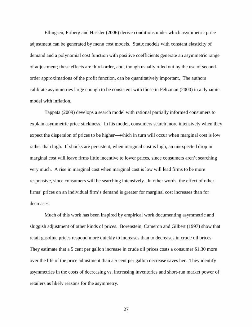
Ellingsen, Friberg and Hassler (2006) derive conditions under which asymmetric price

adjustment can be generated by menu cost models. Static models with constant elasticity of

demand and a polynomial cost function with positive coefficients generate an asymmetric range

of adjustment; these effects are third-order, and, though usually ruled out by the use of second-

order approximations of the profit function, can be quantitatively important. The authors

calibrate asymmetries large enough to be consistent with those in Peltzman (2000) in a dynamic

model with inflation.

Tappata (2009) develops a search model with rational partially informed consumers to

explain asymmetric price stickiness. In his model, consumers search more intensively when they

expect the dispersion of prices to be higher—which in turn will occur when marginal cost is low

rather than high. If shocks are persistent, when marginal cost is high, an unexpected drop in

marginal cost will leave firms little incentive to lower prices, since consumers aren’t searching

very much. A rise in marginal cost when marginal cost is low will lead firms to be more

responsive, since consumers will be searching intensively. In other words, the effect of other

firms’ prices on an individual firm’s demand is greater for marginal cost increases than for

decreases.

Much of this work has been inspired by empirical work documenting asymmetric and

sluggish adjustment of other kinds of prices. Borenstein, Cameron and Gilbert (1997) show that

retail gasoline prices respond more quickly to increases than to decreases in crude oil prices.

They estimate that a 5 cent per gallon increase in crude oil prices costs a consumer $1.30 more

over the life of the price adjustment than a 5 cent per gallon decrease saves her. They identify

asymmetries in the costs of decreasing vs. increasing inventories and short-run market power of

retailers as likely reasons for the asymmetry.

28

Peltzman (2000) documents asymmetries in the responses of output prices to input prices

in micro data from the consumer and producer price indexes, for a total of 77 consumer and 165

producer goods. For both consumer and producer prices, after eight months a one percent

increase in input costs leads to about a half percent increase in output price, but a one percent fall

in input costs only reduces output prices by a bit more than one-third percent. Peltzman also

establishes asymmetric responses in the prices of a supermarket chain, which are more

pronounced for goods with a diverse set of wholesalers or volatile input prices.

D. Other Work on Price Adjustment

Our work is also related to papers that document price stickiness at the microeconomic

level. That work has found a high degree of diversity in the duration of price changes across

goods. Cecchetti (1985) found that magazine prices change every 1½ to 3¼ years. Lach and

Tsiddon (1991) showed that food prices in Israeli supermarkets change every 1.9 months to 1.6

months during periods of high inflation. Kashyap (1995) reported that the average time between

price changes on retail goods in catalogs 15 months, with longer intervals not unusual. Carlton

(1986) show that data from Stigler and Kindahl (1970) on individual transactions prices for

industrial goods indicate average durations of price stickiness of 6.5 months, with, again, many

prices changing even less frequently.. Levy and Young (2004) document that the price of a 6.5

ounce bottle of Coca Cola remained at 5 cents for more than 70 years (1886-1959).

Several more recent studies have used the data underlying the computation of the

consumer price index to show price stickiness for a broader range of goods. Bils and Klenow

(2004) calculate an average duration of price changes of 4.3 months, or 5.5 months including

sales. The duration of price stickiness again differs substantially across price categories.

Nakamura and Steinsson (2006a) find slightly different results. They document that: the median

29

duration of price changes to be 11 months, or 8.7 months for finished goods prices21; one third of

price changes are price decreases.; the frequency of price increases responds to inflation, while

frequency of price decreases and size of price increases and decreases does not; price changes

are highly seasonal (largest in the first quarter, smallest in the fourth quarter); and the hazard

function for price changes is downward sloping for first few months, and flat thereafter, except

for a large spike at 12 months in consumer services. Nakamura and Steinsson (2006b) use the

results of this paper to evaluate the ability of different kinds of price adjustment models to fit the

data. Klenow and Kryvtsov (2005) find a wide distribution of price changes, with some prices

changing monthly while others taking more than 5 years to change.

In our current paper, we find that deposit rates change relatively more frequently than

prices, with median durations of price changes across DIs of about 1 month for CD rates, 3

months for MMDAs, and nearly 5 months for interest checking accounts. The frequency of rate

increases or decreases is linked to the frequency of target federal funds rate changes; since rates

decrease more rapidly than they increase, in long-run equilibrium it is likely that interest rate

increases will be more frequent than decreases.

E. Goods and Service Prices vs. Asset Prices

A simple model of goods and service prices accounts for some key features of deposit

rate behavior. This raises the question of why deposits are more like goods and services in this

respect than they are like other financial assets. One possibility is that, unlike other financial

assets, deposits provide monetary services (also known as liquidity or transactions services).

The asymmetric sluggishness of rates may be an outcome of the factors which move the market

21 Part of the difference between their results and those of Bils and Klenow arises from the definition of a

sale or a temporary price change.

30

for monetary services. The extensive literature on money demand has inversely linked the

opportunity cost of holding deposits—the difference between the rate on some non-monetary

financial asset and the deposit rate—to the level of monetary services provided.22 To the extent

that deposits’ provisions of monetary services is leading to their asymmetric stickiness, one

would expect such stickiness to be greater for assets which provide more monetary services—i.e.

those with greater opportunity costs, or lower rates. Our findings are consistent with that

prediction—deposit rates on MMDAs and interest checking accounts are both lower and stickier

than rates on CDs.

VII. Conclusion

We use a panel dataset of over 2,500 branches of about 900 depository institutions (DIs)

observed weekly over ten years to examine the dynamics of changes in interest rates on interest

checking accounts, MMDAs, and nine different maturities of CDs. We have six key findings.

First, some deposit rates are more flexible than others. CD rates are quite flexible, with the

median branch changing such rates every 6 weeks on average, while MMDA and interest

checking rates show much more inertia, changing every 20 weeks and 37 weeks on average,

respectively. Second, the frequency of rate changes exhibits considerable dispersion for some

types of deposits, with about a quarter of institutions changing interest checking rates twice a

year or less frequently. Third, deposit rate changes are asymmetric: rates adjust about twice as

frequently during periods of falling target federal funds rate than rising ones. Fourth, rates are

uniformly quite sticky during periods when the federal funds rate is flat, with median durations

between price changes ranging from 8 weeks to 39 weeks. Fifth, the median size of rate changes

22 See Barnett, Fisher, and Serletis (1992) for a survey on the microeconomics of demand for monetary

services, and Rotemberg, Driscoll, and Poterba (1995) for one example.

31

is about 11 to 23 basis points, comparable to the typical 25 basis point change in the target

federal funds rate; the distribution of average decreases and increases is about the same, and is

relatively dispersed, with many small changes of a few basis points. Sixth, there is greater

upward stickiness in rates on interest checking and money market accounts for branches of large

DIs than for smaller ones.

These results taken together confirm and extend the earlier findings of Hannan and

Berger (1990), Diebold and Sharpe (1990), and Neumark and Sharpe (1992) on smaller and

shorter datasets, and complement those of Craig and Dinger (2011) and Yankov (2012).

We have two additional results. First, we show that a simple menu cost model is

consistent with the asymmetric stickiness observed here. Second, we show that, even in the

aggregate, deposit rates are sticky, and we estimate some simple models of aggregate rate

adjustment. We use these estimates to show that, when the federal funds rate lifts off from its

current level near zero, deposit rates are likely to follow very slowly, and that depositors could

earn as much as $100 billion less per year relative to what would occur if deposit rates were not

asymmetrically sticky. Of course, these extra payments would come at the expense of bank

revenues, and stickiness of deposit quantities may enhance financial stability. In addition, low

policy rates, by boosting aggregate demand, may have other beneficial effects, so the net welfare

effects of a low interest rate environment are not solely determined by the effects on deposit

holders.

32

REFERENCES

Barnett, William A., Douglas Fisher, and Apostolos Serletis (1992). “Consumer Theory and the Demand for Money.” Journal of Economic Literature, 30(4), pp. 2086-2119.

Barro, Robert J. (1972). “A Theory of Monopolistic Price Adjustment.” Review of Economic Studies, 39(1), pp. 17-26.

Bils, Mark and Peter J. Klenow (2004). “Some Evidence on the Importance of Sticky Prices.” Journal of Political Economy, 112(5), pp. 947-985.

Bricker, Jesse, Arthur B. Kennickell, Kevin B. Moore and John Sabelhaus (2012). “Changes in U.S. Family Finances from 2007 to 2010: Evidence from the Survey of Consumer Finances.” Federal Reserve Bulletin, 98(2), pp. 1-80.

Calvo, Guillermo (1983). “Staggered Prices in a Utility-Maximizing Framework.” Journal of Monetary Economics, 12(5), pp. 1659-1686.

Carlton, Dennis W. (1986). “The Rigidity of Prices.” The American Economic Review, 76 (September), pp. 637-658.

Cecchetti, Stephen G. (1985). “Staggered Contracts and the Frequency of Price Adjustment.” Quarterly Journal of Economics, 100(Supplement), pp. 935-959.

Craig, Ben R., and Valeriya Dinger (2011). “The Duration of Bank Retail Interest Rates.” Federal Reserve Bank of Cleveland Working Paper 10-01R.

Diebold, Francis X. and Steven A. Sharpe (1990). “Post-Deregulation Bank-Deposit-Rate Pricing: The Multivariate Dynamics.” Journal of Business & Economic Statistics, 8(3), pp. 281-291.

Dotsey, Michael, Robert G. King and Alexander Wolman (1999). “State-Dependent Pricing and the General Equilibrium Dynamics of Money and Output.” Quarterly Journal of Economics, 114(3), pp. 655-690.

Eichenbaum, Martin, Nir Jaimovich and Sergio Rebelo (2008). “Reference Prices and Nominal Rigidities.” Working paper, Northwestern University.

Gertler, Mark and John Leahy (2009). “A Phillips Curve with an Ss Foundation.” Journal of Political Economy, 116(3), pp. 533-572.

Golosov, Mikhail and Robert E. Lucas Jr., (2007). “Menu Costs and Phillips Curves.” Journal of Political Economy, 1152), pp. 171-199.

Hannan, Timothy H. and Allen N. Berger (1991). “The Rigidity of Prices: Evidence from the Banking Industry.” The American Economic Review, 81(4), pp. 938-945.

33

Kashyap, Anil K. (1995). “Sticky Prices: New Evidence from Retail Catalogs.” Quarterly Journal of Economics 110(2), pp. 245-274.

Kiley, Michael T. (2000). “Endogenous Price Stickiness and Business Cycle Persistence.” Journal of Money, Credit, and Banking, 32(1), pp. 28-53.

Klenow, Peter and Oleksiy Kryvstov (2008). “State-Dependent or Time-Dependent Pricing: Does It Matter for Recent U.S. Inflation?” Working paper, Stanford University.

Lach, Saul and Dani Tsiddon (1992). “The Behavior of Prices and Inflation: An Empirical Analysis of Disaggregated Price Data.” Journal of Political Economy, 100(2), pp. 349-389.

Levy, Daniel and Andrew T. Young (2004) “`The Real Thing’: Nominal Price Rigidity of the Nickel Coke, 1886-1959.” Journal of Money, Credit and Banking, 36(4), pp. 765-799.

Lucas, Robert E. Jr. (1972), “Expectations and the Neutrality of Money.” Journal of Economic Theory, 4(1), pp. 103-124.

Mankiw, N. Gregory (1985). “Small Menu Costs and Large Business Cycles: A Macroeconomic Model of Monopoly.” Quarterly Journal of Economics, 100(3), pp. 529-539.

----- and Ricardo Reis (2002). “Sticky Information Versus Sticky Prices: A Proposal to Replace the New Keynesian Phillips Curve.” Quarterly Journal of Economics, 117(6), pp. 1295-1328.

Nakamura, Emi and Jon Steinsson (2006a). “Five Facts About Prices: A Reevaluation of Menu Cost Models.” Working paper, Columbia University.

-----(2006b). “Monetary Non-Neutrality in a Multi-Sector Menu Cost Model.” Working paper, Columbia University.

Neumark, David and Steven A. Sharpe (1992). “Market Structure and the Nature of Price Rigidity: Evidence from the Market for Consumer Deposits.” Quarterly Journal of Economics, 107(2), pp. 657-680.

Rice, Tara N. and Evren Ors (2006). “Bank Imputed Interest Rates: Unbiased Estimates of Offered Rates?” Working Paper, Federal Reserve Bank of Chicago.

Rotemberg, Julio (1982). “Monopolistic Price Adjustment and Aggregate Output.” Review of Economic Studies, 58(4), pp. 517-531.

-----, John C. Driscoll and James M. Poterba (1995). “Money, Output, and Prices: Evidence from a New Monetary Aggregate.” Journal of Business & Economic Statistics,13(1), pp. 67-83.

34

Stigler, George and James Kindahl (1970). The Behavior of Individual Prices. National Bureau of Economic Research, General Series, no. 90. New York: Columbia University Press.

Taylor, John B. (1980). “Aggregate Dynamics and Staggered Contracts.” Journal of Political Economy, 88(1), pp. 1-24.

Yankov, Vladimir (2012). “In Search of a Risk-Free Asset.” Working Paper, Federal Reserve Bank of Boston.

0

1

2

3

4

5

6

7

8

9

10

Per

cent

Jan. 1986 Jan. 1988 Jan. 1990 Jan. 1992 Jan. 1994 Jan. 1996 Jan. 1998 Jan. 2000 Jan. 2002 Jan. 2004 Jan. 2006 Jan. 2008

Month

Federal Funds Target Rate

3−Month Treasury Bill Rate

M2 Own Rate

Liquid Deposit Rate

6−Month Small Time Rate

Figure 1Market Rates and Aggregate Rates on M2 and Its Major Components

0

1

2

3

4

5

6

7

8

9

10

Per

cent


Month

Federal Funds Target Rate M2 Own Rate

Figure 2AM2 Own Rate and Federal Funds Rate Target When Funds Rate Target is Falling or Flat

0

1

2

3

4

5

6

7

8

9

10

Per

cent


Month

Federal Funds Target Rate M2 Own Rate

Figure 2BM2 Own Rate and Federal Funds Rate Target When Funds Rate Target is Rising or Flat

0

200

400

600

Num

ber

of D

Is

0 10 20 30 40 50 60 70 80 90 100 110 120

Weeks between rate changes

Median = 7.0 weeksAverage = 9.9 weeks

6−month CDsFull sample

0

200

400

600

Num

ber

of D

Is

0 10 20 30 40 50 60 70 80 90 100 110 120




0

50

100

150

200

Num

ber

of D

Is

0 10 20 30 40 50 60 70 80 90 100 110 120



MMDAFull sample

0

20

40

60

80

100

Num

ber

of D

Is

0 10 20 30 40 50 60 70 80 90 100 110 120



Interest CheckingFull sample

Note: These charts plot the distribution of the average number of weeks between rate changes, by depository institution (DI).For example, on the chart for MMDA rates over the full sample, about 220 DIs averaged 12 to 14 weeks between price changes.

Figure 3: Distribution of number of weeks between rate changes, all branches

0

200

400

600

Num

ber

of D

Is

0 10 20 30 40 50 60 70 80 90 100 110 120



6−month CDsTarget fed funds rate falling

0

50

100

150

200

250

Num

ber

of D

Is

0 10 20 30 40 50 60 70 80 90 100 110 120



6−month CDsTarget fed funds rate rising

0

100

200

300

400

Num

ber

of D

Is

0 10 20 30 40 50 60 70 80 90 100 110 120



6−month CDsTarget fed funds rate flat

0

200

400

600

800

Num

ber

of D

Is

0 10 20 30 40 50 60 70 80 90 100 110 120




0

50

100

150

200

250

Num

ber

of D

Is

0 10 20 30 40 50 60 70 80 90 100 110 120




0

100

200

300

400

500

Num

ber

of D

Is

0 10 20 30 40 50 60 70 80 90 100 110 120




0

50

100

150

200

Num

ber

of D

Is

0 10 20 30 40 50 60 70 80 90 100 110 120



MMDATarget fed funds rate falling

0

20

40

60

80

100

Num

ber

of D

Is

0 10 20 30 40 50 60 70 80 90 100 110 120



MMDATarget fed funds rate rising

0

50

100

150

Num

ber

of D

Is

0 10 20 30 40 50 60 70 80 90 100 110 120



MMDATarget fed funds rate flat

0

20

40

60

80

100

Num

ber

of D

Is

0 10 20 30 40 50 60 70 80 90 100 110 120



Interest CheckingTarget fed funds rate falling

0

50

100

150

Num

ber

of D

Is

0 10 20 30 40 50 60 70 80 90 100 110 120



Interest CheckingTarget fed funds rate rising

0

20

40

60

80

100

Num

ber

of D

Is

0 10 20 30 40 50 60 70 80 90 100 110 120



Interest CheckingTarget fed funds rate flat

Note: These charts plot the distribution of the average number of weeks between rate changes, by depository institution (DI).For example, on the chart for MMDA rates over the full sample, about 220 DIs averaged 12 to 14 weeks between price changes.

Figure 4: Distribution of number of weeks between rate changes, all branchesTarget fed funds rate falling, rising, and flat

0.00

0.20

0.40

0.60

0.80

1.00

Cum

ulat

ive

shar

e of

DIs

0 5 10 15 20 25

Weeks following rate change

6−month CDsIncrease in target fed funds rate on June 30, 1999

0.00

0.20

0.40

0.60

0.80

1.00

Cum

ulat

ive

shar

e of

DIs

0 5 10 15 20 25


6−month CDsDecrease in target fed funds rate on March 20, 2001

0.00

0.20

0.40

0.60

0.80

1.00

Cum

ulat

ive

shar

e of

DIs

0 5 10 15 20 25


24−month CDsIncrease in target fed funds rate on June 30, 1999

0.00

0.20

0.40

0.60

0.80

1.00

Cum

ulat

ive

shar

e of

DIs

0 5 10 15 20 25


24−month CDsDecrease in target fed funds rate on March 20, 2001

0.00

0.20

0.40

0.60

0.80

1.00

Cum

ulat

ive

shar

e of

DIs

0 5 10 15 20 25


MMDAIncrease in target fed funds rate on June 30, 1999

0.00

0.20

0.40

0.60

0.80

1.00

Cum

ulat

ive

shar

e of

DIs

0 5 10 15 20 25


MMDADecrease in target fed funds rate on March 20, 2001

0.00

0.20

0.40

0.60

0.80

1.00

Cum

ulat

ive

shar

e of

DIs

0 5 10 15 20 25


Interest CheckingIncrease in target fed funds rate on June 30, 1999

0.00

0.20

0.40

0.60

0.80

1.00

Cum

ulat

ive

shar

e of

DIs

0 5 10 15 20 25


Interest CheckingDecrease in target fed funds rate on March 20, 2001

Figure 5: Cumulative weekly response of DI branches to target federal funds rate changes

0

100

200

300

400

Num

ber

of D

Is

0 10 20 30 40 50 60 70 80 90 100110120130140150160170180190200

Average size of change (basis points)

Median = 20 bpsAverage = 33 bps

6−month CDsAverage size of rate increases

0

200

400

600

Num

ber

of D

Is

0 10 20 30 40 50 60 70 80 90 100110120130140150160170180190200



6−month CDsAverage size of rate decreases

0

100

200

300

400

500

Num

ber

of D

Is

0 10 20 30 40 50 60 70 80 90 100110120130140150160170180190200




0

200

400

600

800

Num

ber

of D

Is

0 10 20 30 40 50 60 70 80 90 100110120130140150160170180190200




0

50

100

150

200

Num

ber

of D

Is

0 10 20 30 40 50 60 70 80 90 100110120130140150160170180190200



MMDAAverage size of rate increases

0

100

200

300

400

500

Num

ber

of D

Is

0 10 20 30 40 50 60 70 80 90 100110120130140150160170180190200



MMDAAverage size of rate decreases

0

100

200

300

Num

ber

of D

Is

0 10 20 30 40 50 60 70 80 90 100110120130140150160170180190200



Interest CheckingAverage size of rate increases

0

100

200

300

400

500

Num

ber

of D

Is

0 10 20 30 40 50 60 70 80 90 100110120130140150160170180190200



Interest CheckingAverage size of rate decreases

Figure 6: Distribution of average size of rate change

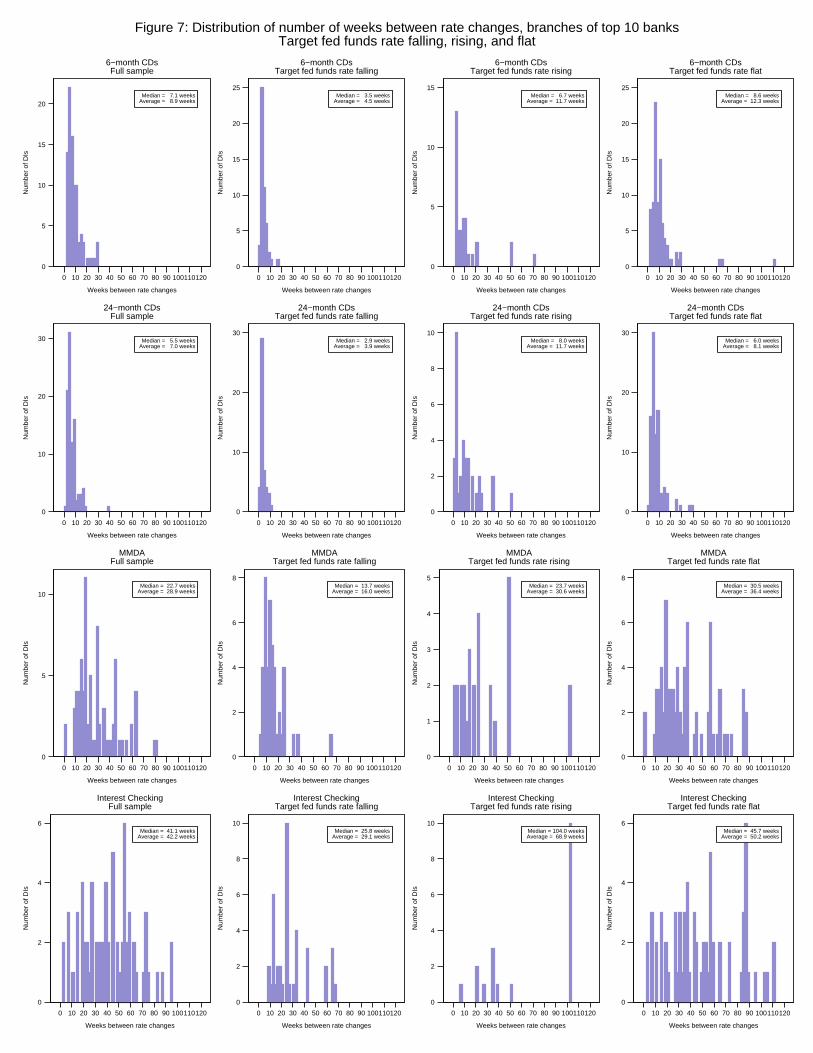
0

5

10

15

20

Num

ber

of D

Is

0 10 20 30 40 50 60 70 80 90 100110120




0

5

10

15

20

25

Num

ber

of D

Is

0 10 20 30 40 50 60 70 80 90 100110120




0

5

10

15

Num

ber

of D

Is

0 10 20 30 40 50 60 70 80 90 100110120




0

5

10

15

20

25

Num

ber

of D

Is

0 10 20 30 40 50 60 70 80 90 100110120




0

10

20

30

Num

ber

of D

Is

0 10 20 30 40 50 60 70 80 90 100110120




0

10

20

30

Num

ber

of D

Is

0 10 20 30 40 50 60 70 80 90 100110120




0

2

4

6

8

10

Num

ber

of D

Is

0 10 20 30 40 50 60 70 80 90 100110120




0

10

20

30

Num

ber

of D

Is

0 10 20 30 40 50 60 70 80 90 100110120




0

5

10

Num

ber

of D

Is

0 10 20 30 40 50 60 70 80 90 100110120



MMDAFull sample

0

2

4

6

8

Num

ber

of D

Is

0 10 20 30 40 50 60 70 80 90 100110120



MMDATarget fed funds rate falling

0

1

2

3

4

5

Num

ber

of D

Is

0 10 20 30 40 50 60 70 80 90 100110120



MMDATarget fed funds rate rising

0

2

4

6

8

Num

ber

of D

Is

0 10 20 30 40 50 60 70 80 90 100110120



MMDATarget fed funds rate flat

0

2

4

6

Num

ber

of D

Is

0 10 20 30 40 50 60 70 80 90 100110120



Interest CheckingFull sample

0

2

4

6

8

10

Num

ber

of D

Is

0 10 20 30 40 50 60 70 80 90 100110120



Interest CheckingTarget fed funds rate falling

0

2

4

6

8

10

Num

ber

of D

Is

0 10 20 30 40 50 60 70 80 90 100110120



Interest CheckingTarget fed funds rate rising

0

2

4

6

Num

ber

of D

Is

0 10 20 30 40 50 60 70 80 90 100110120



Interest CheckingTarget fed funds rate flat

Figure 7: Distribution of number of weeks between rate changes, branches of top 10 banksTarget fed funds rate falling, rising, and flat

0

5

10

15

20

Num

ber

of D

Is

0 10 20 30 40 50 60 70 80 90 100110120130140150160170180190200




0

10

20

30

Num

ber

of D

Is

0 10 20 30 40 50 60 70 80 90 100110120130140150160170180190200




0

5

10

15

20

Num

ber

of D

Is

0 10 20 30 40 50 60 70 80 90 100110120130140150160170180190200




0

10

20

30

40

Num

ber

of D

Is

0 10 20 30 40 50 60 70 80 90 100110120130140150160170180190200




0

5

10

Num

ber

of D

Is

0 10 20 30 40 50 60 70 80 90 100110120130140150160170180190200



MMDAAverage size of rate increases

0

5

10

15

20

Num

ber

of D

Is

0 10 20 30 40 50 60 70 80 90 100110120130140150160170180190200



MMDAAverage size of rate decreases

0

5

10

15

Num

ber

of D

Is

0 10 20 30 40 50 60 70 80 90 100110120130140150160170180190200



Interest CheckingAverage size of rate increases

0

5

10

15

20

Num

ber

of D

Is

0 10 20 30 40 50 60 70 80 90 100110120130140150160170180190200



Interest CheckingAverage size of rate decreases

Figure 8: Distribution of average size of rate change, branches of top 10 banks

sticky deposit rates - board of governors of the federal ... · pdf fileboard of governors....

Documents