stochastic dynamic itinerary interception refueling ... · 6 stochastic dynamic itinerary...

1

Jung, Chow, Jayakrishnan, and Park

UCI-ITS-WP-13-2 1

2

3

4

5

Stochastic dynamic itinerary interception refueling location problem with queue delay for 6

electric taxi charging stations 7

8

9

10

11

UCI-ITS-WP-13-2 12

13

14

15

Jaeyoung Jung, Ph.D. 16

Joseph Y.J. Chow, Ph.D. 17

R. Jayakrishnan, Ph.D. 18

Ji Young Park, Ph.D. 19

20

21

22

Institute of Transportation Studies 23

University of California, Irvine; Irvine, CA 92697-3600, U.S.A. 24

25

[email protected], [email protected], [email protected], [email protected] 26

27

28

29

July, 2013 30

31

32

33

Institute of Transportation Studies 34

University of California, Irvine 35

Irvine, CA 92697-3600, U.S.A. 36

http://www.its.uci.edu 37

mailto:[email protected]

2


1

Stochastic dynamic itinerary interception refueling location with queue delay 2

for electric taxi charging stations 3

4

5

Jaeyoung Jung1*

, Joseph Y.J. Chow2, R. Jayakrishnan

1, and Ji Young Park

3 6

7 1Institute of Transportation Studies, Department of Civil and Environmental Engineering, 8

University of California, Irvine, California, United States 9 2Department of Civil Engineering, Ryerson University, Toronto, Ontario, Canada 10

3Department of National Transport Strategy Planning, The Korea Transport Institute, Gyeonggi-do, 11

Korea 12

13

14

ABSTRACT 15

A new facility location model and a solution algorithm are proposed that feature 1) itinerary-interception 16

instead of flow-interception; 2) stochastic demand as dynamic service requests; and 3) queueing delay. 17

These features are essential to analyze battery-powered electric shared-ride taxis operating in a connected, 18

centralized dispatch manner. The model and solution method are based on a bi-level, simulation-19

optimization framework that combines an upper level multiple-server allocation model with queueing 20

delay and a lower level dispatch simulation based on earlier work by Jung and Jayakrishnan. The solution 21

algorithm is tested on a fleet of 600 shared-taxis in Seoul, Korea, spanning 603 km2, a budget of 100 22

charging stations, and up to 22 candidate charging locations, against a benchmark “naïve” genetic 23

algorithm that does not consider cyclic interactions between the taxi charging demand and the charger 24

allocations with queue delay. Results show not only that the proposed model is capable of locating 25

charging stations with stochastic dynamic itinerary-interception and queue delay, butt that the bi-level 26

solution method improves upon the benchmark algorithm in terms of realized queue delay, total time of 27

operation of taxi service, and service request rejections. Furthermore, we show how much additional 28

benefit in level of service is possible in the upper-bound scenario when the number of charging stations 29

approaches infinity. 30

31

32

KEYWORDS: Electric Vehicle, Shared-Taxi, EV charging, Bi-Level Optimization, Facility Location, 33

Stochastic Demand, Simulation, Refueling 34

35

1. INTRODUCTION 36

Carbon-based emissions and greenhouse gases (GHG) are critical issues that policy-makers have sought 37

to address in a generally global effort since the Kyoto Protocol in 1998. The transportation sector is a 38

major culprit, contributing approximately 30 percent of the GHG emissions in the United States (U.S. 39

EPA, 2006). One technology-oriented solution is to switch vehicle fuels to alternative, sustainable sources 40

and wean consumers off their oil dependency. To that end, automobile manufacturers produced a range of 41

different types of alternative-fuel vehicles (AFVs) including hybrid vehicles (HVs), plug-in hybrid 42

electric vehicles (PHEVs), electric vehicles (EVs), and fuel cell vehicles (FCVs). It has been shown that 43

EVs can cost as little as 1.2 to 1.9 cents per km (2 to 3 cents per mile) compared to 8 cents per km (13 44

* Corresponding Author. Tel.:+1 949-824-5989

E-mail address: [email protected]

3


cents per mile) for vehicles powered by Internal Combustion Engines (ICE), and EVs cause 50 percent 1

less CO2 emissions per mile traveled compared to ICE (Mak et al., 2012). 2

Nevertheless, there are several obstacles to EV adoption; the most important being the chicken-and-3

egg problem related to the electric charging infrastructure. The lack of penetration in the EV market (and 4

other AFVs as well) limits the value of fuel infrastructure investments, which increases the “range anxiety” 5

and reduces consumer demand. As a result, much of the recent research in AFVs has placed optimal 6

location and allocation of refueling infrastructure at the forefront (e.g. Kuby and Lim, 2005; Lin et al., 7

2008; Wang and Lin, 2009; Nourbakhsh and Ouyang, 2010; Kameda and Mukai, 2011; Kang and Recker, 8

2012; MirHassani and Ebrazi, 2012; Chung and Kwon, 2012, Jiang et al., 2012; He et al., 2013; Xi et al., 9

2013). This problem is particularly relevant to EVs because the vehicles tend to have limited ranges, and 10

recharging can take on the order of an hour or more. 11

One implementation strategy is to invest in EV flexible transit services (FTS) (Koffman, 2004) and 12

taxi fleets. FTS encapsulate a wide range of transit and taxi services that include demand responsive 13

transit (DRT), flexi-route transit, car-sharing systems, and ride-sharing. There are several advantages to 14

implementing EV FTS for initial EV adoption: 1) it takes the individual consumer behavior out of the 15

picture since the decision would be based on fleet managers and/or public agencies; 2) “range anxiety” is 16

less of an issue because transit fleets operate in the same urban region; 3) the reduction in energy 17

consumption would be most realized by transit vehicles operating in a congestion-heavy region (Tong et 18

al., 2000) as opposed to long distance rural trips; and 4) specific to FTS, the vehicles can be passenger 19

cars so that the same infrastructure can also serve the consumer market. Even if EVs are not considered 20

ready to replace private ICE vehicles for the general public, they may be viable options for these fleet 21

applications (Barth and Todd, 2001; Better Place, 2012; FedEx, 2012). The Seoul Metropolitan 22

Government in Korea unveiled its “2014 Master Plan for Electric Vehicle” in 2011, which will 23

commercialize 30,000 units of EVs on the road by 2014 with buses and taxicabs (eGlobal Travel Media, 24

2011). One of the key goals in the plan is to deploy 1,000 EV taxicabs by 2014. The EV taxis will be able 25

to operate over a distance of 200 km to 400 km a day and will require battery charging stations or battery 26

replacing facilities. 27

The proliferation of computing and mobile technologies for connected vehicles has made it easier to 28

operate FTS (Lau et al., 2011), resulting in a growing literature in that area: Cortés and Jayakrishnan 29

(2002), Zhao and Dessouky (2008), Hadas and Ceder (2008), Quadrifoglio and Li (2009), Mulley and 30

Nelson (2009), Crainic et al. (2010), Alshalalfah and Shalaby (2012), Nourbakhsh and Ouyang (2012), 31

Kim and Schonfeld (2012), Jung (2012), Jung and Jayakrishnan (2012), and Jung et al. (2013). 32

Surprisingly, there has not been much research in the facility location problem specifically for EV taxi 33

and FTS fleets. 34

Facility location problems for EV transit and taxi fleets have a set of unique characteristics that 35

cannot be addressed by the solutions developed thus far in the literature. First, EV taxis, as service 36

vehicles, need to place much more weight on the cost of the recharging time. Whereas consumers can 37

recharge when they return home for the night, a taxi may need to be out of commission for a significant 38

period of time during the day if it runs out of charge. With limited infrastructure, queue delay is an 39

important problem that has been largely neglected in the AFV facility location literature to date. Second, 40

many of the AFV location problems focused on fuel stations covering paths formed by origin-destination 41

(OD) pairs in a network. However, connected taxis operate with a central dispatch as a dynamic vehicle 42

routing system. In other words, each taxi follows an itinerary that is determined dynamically. Trip-based 43

demand, even modeled with methods such as path flow-interception as described in the next section, 44

cannot capture this dynamic itinerary. Lastly, passenger demand is stochastic, which results in a 45

stochastic dynamic itinerary for each taxi. The AFV location literature has generally ignored such 46

stochastic elements with a few exceptions. 47

A new model is proposed for locating infrastructure for electric taxis: the stochastic dynamic 48

itinerary-interception refueling location problem with queue delay (SDIRQ). The model can also be 49

applied to many other problems in urban logistics. The problem is presented as a bi-level simulation-50

optimization model, and tested on a network in Seoul, Korea spanning 603 km2 (233 mi

2) with 600 51

4


taxicabs, a budget of 100 charging stations, and 22 candidate refueling locations. Section 2 provides a 1

more in-depth literature review to show the motivation. Section 3 presents the bi-level SDIRQ model and 2

two solution methods. A numerical study is provided in Section 4, followed by a conclusion in Section 5. 3

4

2. LITERATURE REVIEW 5

2.1. Refueling Location Problems 6

Facility location problems are optimization models used to determine a set of locations to serve 7

neighboring demand in a network at a minimum or constrained cost. The cost is usually defined by the 8

distances between the demand nodes and the server nodes. These problems have a long history and 9

extensive literature spanning many different fields. Comprehensive reviews and introductions to the 10

subject are available from Owen and Daskin (1998), Drezner and Hamacker (2002), and Snyder (2006). 11

In the studies on conventional-fuel vehicles, it is well recognized that conventional models with 12

node-based demand do not handle the refueling station siting problem very well. This is because people 13

generally will not make a trip from their home to the station solely for refueling. Both Upchurch and 14

Kuby (2010) and Kang and Recker (2012) have convincingly demonstrated this point by comparing 15

against the conventional models. Instead, three alternative approaches have been considered. 16

The first, and the more popular approach, has been the flow-capture or flow-interception location 17

problem (Hodgson, 1990; Berman et al., 1992). The problem is designed as a path-based version of 18

Church and ReVelle’s (1974) conventional maximal covering location problem. The shortest path 19

between each OD pair is considered covered if it passes through at least one node that contains a server. 20

The ij notation is switched to p path notation over the set of all shortest paths between each OD pair. 21

Kuby and Lim (2005) extended the model to a flow-refueling location problem (FRLP), which serves 22

demand from origin-destination flows along their shortest paths rather than demand at their end points. 23

FRLP selects optimal refueling locations to maximize coverage of the these flows by considering vehicles 24

traveling the full round trip path with a range constraint not present in the prior formulation. Kuby and 25

Lim (2007) further extended the problem to allow solutions on arcs because the optimality condition of 26

being on nodes was only true for the flow-interception problem, not the range-constrained flow-refueling 27

location problem. Upchurch et al. (2009) added capacity constraints to the problem. Kim and Kuby (2012) 28

relaxed the FRLP to allow penalized or maximum deviations from the shortest paths to get to fuel stations. 29

Jiang et al. (2012) proposed a flow-based model that combined capacity as well as deviation flow. 30

Because of the need to enumerate facility combinations, the FRLP was not very tractable. Wang and 31

Lin (2009) proposed a variant path-based set covering model that avoided the combination enumeration 32

by using variables to track remaining fuel and range. Wang and Wang (2010) further combined path and 33

node-based passenger demand as a multiobjective problem. Capar and Kuby (2012) reformulated their 34

model in an effort to make it more efficient, also resorting to constraints based on range variables. 35

MirHassani and Ebrazi (2012) proposed a new model based on both Kuby’s and Wang’s models that was 36

more computationally efficient. Their model was extended by Chung and Kwon (2012) to handle multi-37

period staging of investment strategies. 38

A second approach is to ignore ODs altogether and just relate the value of a location based on 39

vehicle-miles traveled (VMT) indicators (Lin et al., 2008). While this simplifies the problem somewhat, it 40

ignores the range from a given location to a fuel station and simplifies assumptions about the probability 41

of a particular vehicle’s location. 42

The third and most recent approach is to locate based on an itinerary, or trip chain of multiple ODs, 43

instead of just a trip OD. Nourbakhsh and Ouyang (2010) integrated the path-based refueling location 44

problem with the fuel scheduling problem for freight locomotives, which was an initial step in this 45

direction in the refueling literature. Kang and Recker (2012) introduced a model to locate hydrogen 46

stations where households respond to location decisions by rescheduling their daily itineraries using an 47

activity-based variant of the pickup and delivery problem (Recker, 1995). This approach is more high 48

5


resolution than the trip-based location solutions because it includes departure and arrival times throughout 1

the day and maintains trip chains for each household member. It is the first study of an itinerary-2

interception refueling location model. The model is based on the location-routing problem (Perl and 3

Daskin, 1985; Laporte et al., 1988), and has been generalized to an activity-based network design 4

problem (Kang et al., 2013). The differences between these classes of models and their hypothetical 5

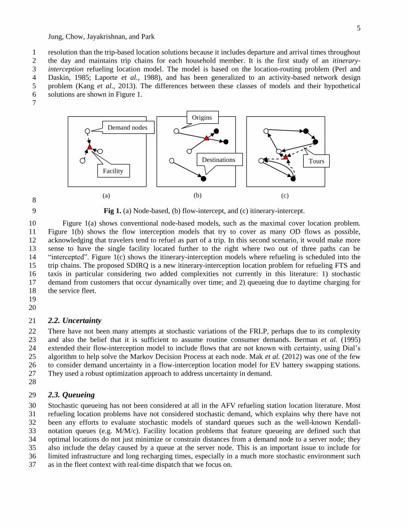
solutions are shown in Figure 1. 6

7

8

Fig 1. (a) Node-based, (b) flow-intercept, and (c) itinerary-intercept. 9

Figure 1(a) shows conventional node-based models, such as the maximal cover location problem. 10

Figure 1(b) shows the flow interception models that try to cover as many OD flows as possible, 11

acknowledging that travelers tend to refuel as part of a trip. In this second scenario, it would make more 12

sense to have the single facility located further to the right where two out of three paths can be 13

“intercepted”. Figure 1(c) shows the itinerary-interception models where refueling is scheduled into the 14

trip chains. The proposed SDIRQ is a new itinerary-interception location problem for refueling FTS and 15

taxis in particular considering two added complexities not currently in this literature: 1) stochastic 16

demand from customers that occur dynamically over time; and 2) queueing due to daytime charging for 17

the service fleet. 18

19

20

2.2. Uncertainty 21

There have not been many attempts at stochastic variations of the FRLP, perhaps due to its complexity 22

and also the belief that it is sufficient to assume routine consumer demands. Berman et al. (1995) 23

extended their flow-interception model to include flows that are not known with certainty, using Dial’s 24

algorithm to help solve the Markov Decision Process at each node. Mak et al. (2012) was one of the few 25

to consider demand uncertainty in a flow-interception location model for EV battery swapping stations. 26

They used a robust optimization approach to address uncertainty in demand. 27

28

2.3. Queueing 29

Stochastic queueing has not been considered at all in the AFV refueling station location literature. Most 30

refueling location problems have not considered stochastic demand, which explains why there have not 31

been any efforts to evaluate stochastic models of standard queues such as the well-known Kendall-32

notation queues (e.g. M/M/c). Facility location problems that feature queueing are defined such that 33

optimal locations do not just minimize or constrain distances from a demand node to a server node; they 34

also include the delay caused by a queue at the server node. This is an important issue to include for 35

limited infrastructure and long recharging times, especially in a much more stochastic environment such 36

as in the fleet context with real-time dispatch that we focus on. 37

Demand nodes

Facility

Origins

Destinations Tours

(a) (b) (c)

6


One of the earliest efforts to incorporate queues in a location model is Larson’s (1974) hypercube 1

queueing model. More recently, Boyaci and Geroliminis (2011) extended the model to handle large scale 2

spatial queueing. Spatial queueing treats the whole coverage of demand as a service, and are more 3

appropriate for mobile servers that relocate from one node to another. 4

For stationary location siting that covers a large neighborhood of nodes, the challenge is to find some 5

way to quantify the steady state delay at a server node to include in the objective function. This is trivial 6

for single server nodes that assume Markov arrivals and service times, but becomes cumbersome for 7

multiple co-located servers. In AFV refueling location problems, there is usually a set number of 8

refueling or charging stations at a given server node. It becomes a highly nonlinear function of the 9

demand arriving at the server node, which leads to an intractable facility location problem if it is included 10

in the objective function. In a special context of emergency vehicles’ dispatch, Marianov and ReVelle 11

(1996) linearized this expression by moving it to the constraint of a maximal availability location problem 12

(MALP) and showing how an equivalent linear form relative to a reliability measure can be obtained. 13

Marianov and Serra (1998) further extended the linearized queueing constraint to other location models. 14

To date, there has not been such an extension to the path-based FRLP, much less to itinerary-based 15

demand. 16

A similar area of research is on an allocation problem that considers queueing. In this problem, the 17

locations are already set and the problem is to allocate the demand to the server nodes (or to allocate 18

servers to given demand) in an optimal manner. For example, Xi et al. (2013) proposed an allocation 19

model with exogenous deterministic demand using simulation to evaluate the deterministic multiple-20

server delay and level of service. The allocation problem with stochastic queueing is even more 21

challenging and has its roots in queueing networks, where researchers sought to determine the optimal 22

allocations of servers in a network to minimize total network cost. Approximations for the multiple server 23

delay evaluation were considered very early on. Iglehart (1965) presented a proof of an approximation for 24

an M/M/c model. Rolfe (1971) extended the approximation to M/D/c queues with deterministic service 25

times. Kimura (1983) generalized the approximation to M/G/c queues. Lovell et al. (2012) introduced a 26

continuum approximation approach to approximate M/M/1 queues. 27

Berman and Drezner (2007) proposed a multiple server allocation model that accounted for queues at 28

the server nodes, assuming demand is allocated to the closest server node. The multiple server allocation 29

problem can be solved exactly using a greedy algorithm to incrementally assign servers, as has been 30

demonstrated in the queueing network literature (e.g. Rolfe, 1971). 31

32

2.4. Shared-Taxi Operations 33

In short, the literature on AFV refueling stations has been growing in recent years but they have dealt 34

primarily with consumer passenger vehicles, using deterministic approaches that do not account for 35

queueing. Furthermore, one investment strategy that may help overcome the chicken-and-egg problem—36

investing in publicly operated or regulated AFV fleets and infrastructure to primarily support them—has 37

been largely disregarded. Investing in infrastructure for public fleets can reduce the risk of lack of 38

demand. At the same time, the infrastructure would provide a positive feedback force that could drive the 39

demand for the consumer AFV market. 40

Jung and Jayakrishnan (2012) showed that the shared-ride taxi (or shared-taxi) is a less constrained, 41

and hence more generalized, operation than the standard taxi. A shared-taxi allows different groups of 42

passengers to share a taxi ride. This trend is gaining traction in many countries in Asia. In China, the 43

Beijing government recently allowed taxi-sharing due to the shortage of taxicabs during rush hours 44

(China.org, 2012). In Singapore, Taiwan, and Japan, dynamic shared-taxi services are provided to link 45

passengers who travel to the same area (Asiaone, 2012; Tao, 2007; Tsukuda and Takada, 2005). 46

Jung and Jayakrishnan (2012) proposed a real-time shared-taxi system operated by an online 47

dispatch center with the help of communication technologies and geo-location services. The advanced 48

shared-taxi service is capable of taking random service requests and updating vehicle schedules. Further 49

7


details of the shared-taxi concept and simulation procedure, as well as a more in-depth review of the 1

shared-taxi literature, are given by Jung and Jayakrishnan (2012). 2

3

2.5. BEV Taxi Charging 4

Unlike HEVs or PHEVs, BEVs are powered exclusively by the electricity from its battery pack. Most 5

prevailing 5-seater vehicles produced by major automobile manufacturers are equipped with up to 24 6

kWh battery types that allow up to a maximum of 100 miles per charge depending on driving conditions. 7

The EV charging station is commonly called EVSE (Electric Vehicle Supply Equipment), which has three 8

levels of SAE (Society of Automotive Engineers) classification: (1) Level 1 with 120 volt outlet; (2) 9

Level 2 with 240 volts; and (3) Level 3 with higher voltage DC power for fast charging, which takes less 10

than one hour. These considerations are made in the computational study in Section 4. 11

12

3. PROPOSED MODEL 13

The SDIRQ model simultaneously seeks a set of locations and number of co-located servers at each of 14

those locations to minimize the average delay—defined as the sum of travel to a facility, wait time at the 15

facility to be served, and service time—for a set of random demand itineraries. This type of problem has 16

many applications where demand can be characterized as an itinerary of trip chains that occur with a 17

degree of uncertainty, including taxi fleets, activity based land use planning, military logistics, supply 18

chain logistics, humanitarian logistics, among others. The specific application addressed in this study is 19

the location of charging stations to minimize the delay to taxi fleets’ itineraries, which are dependent on 20

random customer arrivals over time. A simulation-based optimization problem formulation is presented to 21

characterize this problem. 22

23

3.1. SDIRQ Model Formulation 24

Given the complexity of the shared-taxi operations, the location model is formulated as a bi-level problem. 25

Bi-level programming problems split the decisions of the system planner (leader) and the system users 26

(followers) into two levels so that the sub-problems are solvable and an iterative approach can be used to 27

arrive at a local optimum. The upper-level problem is defined by 28

29

30

Subject to 31

32

33

Where is implicitly determined in the lower-level problem 34

35

36

Subject to 37

38

39

where and are the objective function and constraint set of the upper-level; and are for the lower-40

level problem. The decision variables and are defined for the upper level and lower level, respectively. 41

8


In the case of the stochastic dynamic itinerary-interception refueling location problem with queue 1

delay (SDIRQ), the master problem is split into an 1) upper level server allocation problem with queue 2

delay, and a 2) lower level stochastic dynamic itinerary simulation. 3

4

3.1.1. Upper Level Formulation 5

The upper level problem is based on Berman and Drezner’s (2007) multiple server allocation problem. 6

The objective is to minimize the sum of the travel times and the average queue delays at each server node 7

for all taxis. A complete graph with a set of nodes and a set of links is 8

considered. At each node , demand is generated at a rate of per time unit (e.g., an hour). This 9

demand is obtained from the output of the lower level problem. The service rate of each server is 10

customers per time unit with a maximum of servers on the network. The set of nodes which are 11

assigned servers (server nodes) has a cardinality of , which means that some of the nodes may not 12

have servers. is defined as the set of closest nodes in to a node in , resulting in Equation (1) to 13

determine the arrival rate at a service node . 14

15

(1) 16

17

The total travel times from demand nodes to all server nodes are modeled as a p-median objective. 18

is defined as the expected time spent at a server node with servers when the arrival rate is 19

and the service rate is , where is greater than or equal to one. The vector is the 20

assignment of servers to the set . The queue delay at each location can be represented as an M/M/ 21

queueing system. The upper level objective function is then expressed as Equation (2), as shown in 22

Berman and Drezner (2007). 23

24

(2) 25

26

subject to 27

28 (3) 29

30

Unlike Berman and Drezner’s study, we assume that all demand nodes can be server nodes. Since is 31

not predefined in our study, the solution algorithm shown in Section 3.2 includes a consolidation process 32

in which servers at a lower demand node can be consolidated with another node if it reduces the total 33

queue delay. We set up an additional constraint for the maximum number of servers, , at node due 34

to the geographical limitations of EV charging locations in an urban area. 35

36

(4) 37

38

As pointed out by Pasternack and Drezner (1998), higher values of utilization ( ) may cause 39

small (the probability of no customers in the system) when calculating (the average waiting time) in 40

the standard way. Lower values of can cause computational overflows for subsequent calculations of 41

(the average queue length) and . The same recursive method is used for the queue delay. For a given 42

, , and , the queue delay time can be obtained in a recursive manner shown in Equations (5) and (6). 43

44

;

(5) 45

46

and 47

48

9


(6) 1

2

3.1.2. Lower Level Problem 3

The lower level problem, is replaced with a simulation similar to the recharging schemes previously 4

designed for HCPPT by Jung and Jayakrishnan (2012). Because this problem requires great flexibility of 5

implementing various types of vehicle routing algorithms and vehicle controls for door-to-door passenger 6

services, which are not available in most commercial transportation simulation tools. However, there is a 7

significant difference that needs to be considered. An EV taxi is assumed to visit a charging station only 8

after completion of passenger delivery (similar to the assumption made by Kameda and Mukai (2011) for 9

shared-buses in Tokyo). EV taxi charging is added as event at the end of vehicle schedule within the 10

current driving range, but the event can be considered at any time step in the vehicle’s movement. We 11

assume that the dispatch algorithm is provided with the locations of charging stations so that it can 12

determine when a connected taxi should be replenished and which station the taxi should visit. New 13

pickup and delivery events are prohibited if the vehicle is already headed to a charging station or if the 14

vehicle has higher risk of being discharged when the new schedule is performed given the remaining 15

range. Further details can be found in Jung et al. (2013). 16

A simulation rule is used to insert a charging station visit when a taxi reaches a threshold and no 17

passenger is being served. For battery charging, a vehicle tries to find the closest charging locations to 18

minimize the travel distance and risk of being discharged after finishing its final delivery. The lower-level 19

simulation generates a unique charging profile and queue delay at each charging location as well as a 20

system performance for shard-taxi operation. The simulation time is set to be long enough so that vehicles 21

need to visit charging stations multiple times. Since the stochastic taxi demand is determined by a 22

simulation seed number, multiple sets of simulations are conducted for each iteration to minimize the 23

random effect. 24

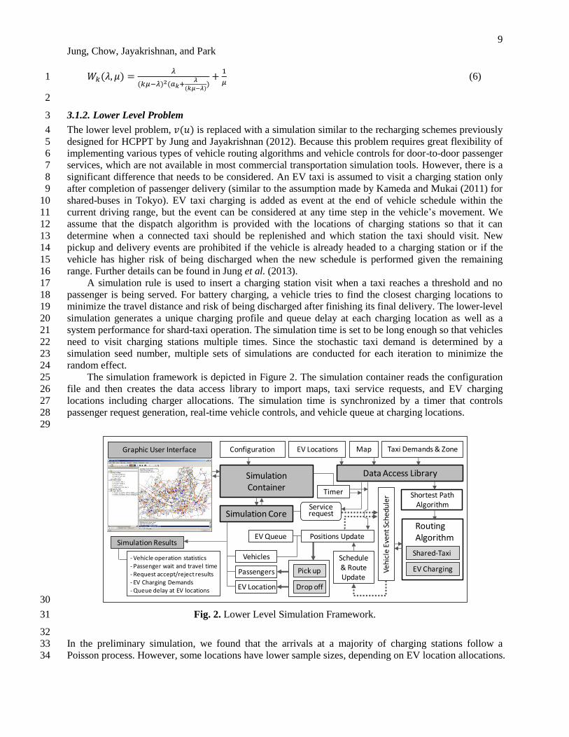
The simulation framework is depicted in Figure 2. The simulation container reads the configuration 25

file and then creates the data access library to import maps, taxi service requests, and EV charging 26

locations including charger allocations. The simulation time is synchronized by a timer that controls 27

passenger request generation, real-time vehicle controls, and vehicle queue at charging locations. 28

29

30

Fig. 2. Lower Level Simulation Framework. 31

32

In the preliminary simulation, we found that the arrivals at a majority of charging stations follow a 33

Poisson process. However, some locations have lower sample sizes, depending on EV location allocations. 34

Map Taxi Demands & ZoneConfiguration

SimulationContainer

Graphic User Interface

Data Access Library

Simulation Core

Vehicles Shared-Taxi

Positions Update

Shortest PathAlgorithm

Pick up

Drop off

Routing Algorithm

Veh

icle

Eve

nt S

ched

ule

r

EV Locations

Schedule& RouteUpdate

Servicerequest

Timer

EV Charging

EV Queue

EV Location

Passengers

Simulation Results

- Vehicle operation statistics- Passenger wait and travel time- Request accept/reject results- EV Charging Demands- Queue delay at EV locations

10


The lower samples are not enough to estimate the arrival rates because they can produce very noisy 1

estimates. Second, the translated demand rate should always be less than the service rate according to the 2

assumption made in the upper level (steady state intensity less than one). In other words, the basic inverse 3

function shown in Equation (7) can fail in the upper level problem. 4

5

(7) 6

7

The lower level simulation provides the number of servers , service rate , and queue delay time for 8

each location. To address the intensity issue, an inverse interpolation method is used to approximate the 9

corresponding demand rate so that the queue delay function in Equation (6) is continuously and 10

monotonically increasing within an interval in which there is a single-valued inverse. A 11

bisection method is applied to compute the inverse given the stable utilization interval. 12

13

3.1.3. Bi-Level Interactions 14

The iteration between the upper and lower level problems captures the cyclic effect that queue delay has 15

on the dispatch of the taxi fleet, which in turn determine the demand patterns for the charging stations, 16

resulting in the allocation of chargers that impact that queue delay. Figure 3 describes the iterative 17

procedure for the simulation-optimization-based EV charger location problem. First, servers are evenly 18

distributed over the candidate charging locations, and then the lower level simulation is called. The lower 19

level simulation tracks all vehicle pickups, dropoffs, queueing, and charging events including which 20

charging location is used. After the first run of lower level simulation, the charging profiles and queue 21

delay are collected and transferred to the upper level problem. The upper level problem assigns servers 22

optimally to minimize queue delay and travel time. Once the upper level problem is solved, the optimal 23

allocation of chargers is compared with the previous allocation status. If there is no change, the procedure 24

ends with the current charger allocation on candidate locations; otherwise, the lower level simulation is 25

called with the updated charger allocation. 26

27

11


1

Fig. 3. Bi-Level Procedure for EV charger allocation. 2

3

A solution method is presented to solve this bi-level problem in Section 3.2. The method is based on a 4

modification of Berman and Drezner’s (2007) allocation algorithm. This solution method is compared to 5

a benchmark single level solution method presented in Section 3.3. The benchmark method uses a genetic 6

algorithm to assign chargers without considering any iterative interaction of queue delays in the upper 7

level with the demand assignment in the lower level. It is used to validate the benefit of considering queue 8

delay in the SDIRQ. 9

10

3.2. Proposed Solution Method – Bi-level 11

The solution of the upper level uses a modification of Berman and Drezner’s (2007) Algorithm 1 that 12

includes a consolidation procedure discussed in Section 3.1. At this level, the demand obtained directly 13

from the lower level is assumed constant. 14

15

Proposed Upper Level Algorithm: (steps 1-4 are from Berman and Drezner (2007)) 16

1. For each node , find the minimum number of servers necessary to service the demand. This 17

minimum number is 18

2. If , then there is no feasible solution. 19

3. If , check the decrease in queue delay by changing to . If , increase the 20

number of servers by one at the node with the maximum time decrease. 21

4. Repeat until . 22

Lower-Level EV Shared-taxi simulation

Minimize Passenger wait and travel time

Subject to Limited EV charging locations Limited EV taxi driving ranges Maximum passenger waiting time Maximum passenger detour length

EV charger allocation of l-th iteration,

Re-allocate EV chargers with

Estimate charging demand at each charging location i

Initial assign of EV chargers on candidate locations Assume that all candidate locations are considered and all available

chargers are randomly distributed on the candidate locations.

Upper-Level Multiple Server Allocation Problem

Minimize Total queue delay and travel time

Subject to Number of EV chargers to allocate Maximum EV chargers for each location

Final allocation of EV chargers for candidate locations The candidate locations assigned no chargers are not considered for

EV charging locations.

Stop iteration with

NO

YES

SIMULATION

INPUT

12


5. For each node , find the closest server node with 1 or more servers, and compare the current 1

objective value with relocating demand and servers to the adjacent node with and 2

and considering travel cost . If and the objective value of relocating decreases, set 3

node and as a candidate node pair. 4

6. Find a best node pair among the candidate node pairs to minimize the objective function, then 5

consolidate node to node . 6

7. Repeat the step 5 and 6 until there is no improvement in the objective value. 7

8

We also propose an improvement to the dispatch algorithm from Jung and Jayakrishnan (2012). The 9

original insertion heuristic starts by comparing all vehicles to find a best vehicle to minimize both 10

passenger travel time and waiting time. However, the algorithm is computationally inefficient when both 11

service area and fleet size are large. 12

The proposed algorithm consists of two steps. First, once a new passenger request, ( ) comes in, 13

the system selects available vehicles in the corresponding geographical zonal area to insert a new trip 14

request. Each passenger trip is identified by its origin and destination. In this stage, available vehicles are 15

filtered to prevent excessive computational burdens. At the second stage, the algorithm seeks the best 16

vehicle to minimize service wait time and travel time of the new passengers as well as the previously 17

assigned passengers. In this lower level simulation, the allocation of charging stations is obtained directly 18

from the upper level and assumed fixed. 19

20

Proposed Lower Level Dispatch Algorithm 21

Stage 1: Identify the zonal area of the new passenger request, , then prepare a vehicle set based on ’s 22

trip points and time windows. 23

24

Stage 2: Find the best vehicle , satisfying the following objective function to insert -th and 25

-th for the new request in equation (5). 26

27

– (5) 28

29

(6) 30

31

(7) 32

33

where 34

35

= new request from passenger , 36

= set of pickup and dropoff events in vehicle vehicle ’s schedule 37

= incremental cost of vehicle j for inserting a new request zi 38

= current total cost of vehicle ’s with schedule 39

= waiting time (cost) associated with -th event in 40

= in-vehicle time (cost) associated with -th event in 41

= total cost of vehicle when adding a new request 42

, = -th pickup and -th dropoff insertion positions for vehicle ’s minimum cost with 43

44

In stage 2, equations (6) and (7) denote the travel cost based on vehicle ’s current itinerary and the 45

updated cost by assuming that the new request is inserted into an optimal position among the existing 46

pickup and dropoff events. When inserting a new request, all previously assigned events should be kept 47

13


within the constrained time windows. If there are no more available vehicles to consider, the dispatch 1

algorithm assigns the new request to the vehicle with minimum incremental cost, . Otherwise, the 2

passenger request is rejected due to the constraint. The dispatch algorithm is then combined with the 3

recharging scheme by Jung et al. (2013). 4

5

3.3. Single-level Solution Method 6

The single-level procedure is proposed as a baseline algorithm without the cyclic interaction of queue 7

delay and demand between the upper and lower level. This method consists of simply evaluating 8

simulation outputs of different EV charger allocation schemes and using Genetic Algorithm (GA) to 9

improve the fitness of the population of solutions. Unlike the bi-level method, the direction finding is 10

based purely on fitness function that includes queue delay, but no update of that cost is present in the 11

simulation. This baseline algorithm is designed to show what happens if no queueing is considered by the 12

taxi fleet dispatch even though the cost exists. 13

14

Single-level procedure 15 16

Step 1: EV charging demand allocation for each location is achieved from the lower level simulation by 17

relaxing the queue delay constraint. 18

19

Step 2: The multiple server allocation problem is applied to allocate EV chargers. 20

21

In Step 1, it is assumed that enough chargers are installed at each location so that vehicles start battery 22

charging without the queue delay effect when they visit charging locations. This approach provides a 23

viable option in the sense that one can estimate the upper bound of potential EV charging demands when 24

the deployment size is not determined yet (Jung and Jayakrishnan, 2011). However, such an upper bound 25

can be seriously overestimated especially when the charging frequency of EV fleet operation is higher. As 26

a result, the server allocation problem in Step 2 might end up with an infeasible solution that has a higher 27

demand rate than the service rate. 28

GAs have great flexibility to solve the combinatorial optimization problem with complex 29

contratins. Although GAs do not guarantee optimal solutions, they are efficient in seeking approximate 30

solutions in NP-hard problem. The solution procedure employs an initial population, selection, elitism, 31

crossover, and mutation. Figure 4 provides an illustrative example of chromosome encoding and genetic 32

operators designed for the single level procedure with five candidate locations. In figure 4(b), as the 33

crossover operation may produce an infeasible solution – having more or less chargers in total, an 34

additional modification procedure is required to keep the same total number of chargers. The modification 35

procedure adds or subtracts additional chargers on a random position to keep the total number of chargers 36

the same. 37

The EV charging demands from simulation results are translated into the demand rates because there 38

is no queue delay measured in the simulation results with infinite numbers of servers. Instead, a finite 39

number of servers are assumed to consider queue delay at each charging location. If the demand rate goes 40

over the service rate given by the number of servers at a location, a penalty value, , is applied with a 41

linear relationship of queue utilization, , as shown in Equations (8) and (9). 42

43

(8) 44

45

where 46

47

(9) 48

49

14


1

2 (a) Chromosome Encoding 3

4 (b) Crossover 5

6 (c) Mutation 7

8

Fig. 4. Chromosome Encoding and Genetic Operators in GA. 9

10

4. COMPUTATIONAL STUDY 11

The goal of the computational study is to compare the performance of the proposed bi-level solution 12

algorithm against the benchmark “naïve” single-level GA approach. Because stochastic dynamic shared-13

taxi dispatch can only be evaluated as an itinerary, the earlier models of flow-interception or even node-14

based location models cannot be run without making crippling assumptions. In addition, the improvement 15

of deterministic itinerary-interception models against node-based models has already been documented in 16

Kang and Recker (2012). This comparison was to demonstrate the feasibility and the performance of the 17

bi-level algorithm with and without the cyclic interaction between the demand and the allocation with 18

queue delay that is present in the method. 19

20

4.1. Study Setting and Parameters 21

In this study, the Renault-Samsung SM3 Z.E. is assumed, which is a model built by Renault-Samsung 22

Motors for South Korea, based on the Renault Fluence Z.E. Renault-Samsung claims that the SM3 Z.E. is 23

outfitted with a 24 kWh lithium-ion battery with a maximum range of 115 mile (184 km) measured on the 24

NEDC (New European Driving Cycle) combined cycle, which is similar to Nissan LEAF. A “QuickDrop” 25

system (known as battery swapping) allows the discharged battery to be replaced quickly with a fully 26

charged one at a dedicated EV battery switch station. In addition, a fast charging system using a 32A 27

400V 3-phase supply enables the battery to be charged in 45 minutes. Since an official Korean range 28

specification is not yet established, we assume conservative average ranges of 112 km (70 miles) on 29

highways and 128 km (80 miles) on city traffic with a 16-km range of random variation for each 30

individual vehicle. 31

Stochastic taxi demand is obtained from an EMME/2 transportation planning model developed at the 32

Korea Transportation Institute (KOTI). As of 2011, trip demand consists of automobile, bus, subway, rail, 33

taxi, and other types of demand, which cover Seoul with a total of 560 centroids over 603 km2 (233 mi

2). 34

Under the usual assumption of spatial uniformity of demand around a zone centroid, point-to-point taxi 35

k1 k2 k3 k4 k5 Number of chargers at each location, ki

Gene 1

Chromosome

2 0 2 1 5

0 1 4 2 3

0 1 2 1 5

2 0 4 2 3

1 1 2 1 5

1 0 4 2 3

Crossover Modification

Parent 2

Parent 1

Offspring 2

Offspring 1+1

-1

0 1 4 2 3

Position 1

Position 2Mutation

2 1 4 0 3

Swapped

15


demands are randomly generated in accordance with destination probabilities of the taxi demand table in 1

each centroid. The point-to-point demands are projected to the nearest road segment with its direction for 2

door-to-door services except on limited-access roads. Real-time service requests arrive according to a 3

Poisson process in a temporal manner. Figure 5(a) presents the spatial distribution of taxi demands 4

including both origins and destinations used for stochastic trip requests for an 8-hour simulation with the 5

minimum trip length of 1.0 km for taxi service. In figure 5(b), a total of 22 candidate charging stations on 6

5 km by 5 km reference grid cells are assumed over the road network in the EV taxi simulator. One 7

hundred chargers are evenly distributed over the 22 candidate locations in the initial simulation setup. 8

9

10

11

(a) Distribution of Stochastic Taxi Demand 12

13

(b) EV Charging Locations and Transportation Network in Seoul 14

Fig. 5. Taxi Demands, EV Charging Locations on Transportation Network. 15

16


1

According to the statistics from Seoul Taxi Association, a taxi carries more than 35 passengers each day 2

on average. The average travel distance is over 250 km/day and 5 km/trip, with a significant portion of the 3

travel distance being non-revenue segments when the taxis travel empty for the pickups. A total of 72,000 4

taxi licenses are registered including owner-driver taxi and a total fleet of 40,000 vehicles due to the taxi 5

rotation system to restrict the number of operating taxicabs operating as of 2011. Shared-taxis are 6

prohibited by regulations in Korea, but it is publicly known that many taxicabs carry multiple passenger 7

groups at the same time if they are traveling to the same destination because of limited supply. It is 8

assumed that EV taxi service offers dynamic shared-ride for passengers in order to increase its system 9

performance. According to 2014 Master Plan for Electric Vehicle by Seoul, Korea, the city plans to 10

deploy around 30,000 commercial EVs including buses, taxis, and private vehicles. Since it is expected 11

that EV taxi will be able to operate over a distance of 200 km to 400 km a day, Seoul seeks to initially 12

establish replenishing stations with high-speed charging (SAE Level 3) or battery replace facilities. 13

In this study, 600 taxicabs are initially considered for electrification, which is equivalent to 1.5% of 14

the total number of vehicles operated in Seoul. The initial positions of vehicles are randomly generated 15

over the simulation area. The simulation time is set to 8 hours including 30-min as a warm-up period, 16

which is assumed to include peak operating hours. An average of 1-min boarding and alighting times are 17

assumed for each passenger, which is based on a random uniform distribution U(0.5, 1.5). At each lower 18

level simulation step, ten simulation sets are conducted by choosing ten different seed values. 19

In the shared-taxi scenario, we set maximum waiting time (900 sec) and maximum detour length 20

(maximum 1.2 times of door-to-door travel distance) for passenger time windows. A taxicab can carry a 21

maximum of four passenger groups at the same time, which provides a realistic scenario rather than 22

having three or more groups. The charging time is assumed to be exponentially distributed with an 23

average of 45 minutes. From our preliminary simulation, the majority of generated trip demands are 24

within 10 km. The average trip length is 6.4 km and the expected door-to-door travel time 13.4 min under 25

the assumption that vehicles can travel at 60~90% of the posted speeds on the network. 26

Two initial charging strategies are possible, one starting with fully charged EVs (FISOC: Full Initial 27

Sates of Charge) and the other with randomly charged EVs (RISOC: Random Initial State of Charge) at 28

the beginning of the simulation. Jung (2012) found that charging demands tend to be concentrated at 29

certain times during the simulation when the eight hour period started with fully charged vehicles, so 30

RISOC is assumed in this study. This study provides four different scenarios: (1) Single-level approach; 31

(2) Bi-level approach; (3) Infinite chargers intended to relax charging delay factors; and (4) Non-EV 32

operation with conventional ICE taxicabs. 33

34

Table 1 35 Scenarios for computational study. 36

EV Shared-taxi simulation

Shared-taxi settings Service area (km

2)

Simulation time (hours) / Warm up (hours) Number of service vehicles Vehicle capacity (seats/vehicle) Number of centroids (zonal areas) Max. wait time (min) / Max. detour factor Vehicle types

EV settings Battery Capacity

1 (kWh) / Battery Charging Time (average min)

Ranges (km) Number of charging stations (/each candidate location) Charging schemes Candidate EV locations / Max. available chargers EV Charging Operations

605

8.0 / 0.5 600

4 560

15 / 1.2 EV / ICE

24 / 45

112 (Highway) / 128 (City Traffic) Min. 0 – Max. 20 chargers

Random Initial State of Charge (RISOC) 22 / 100

Single-level, Bi-level, Infinite Chargers, Non-EV 1 Battery pack capacity (kWh): kilowatt-hour(s) 37

17


1

4.2. Results 2

The system performance of the lower level simulation is calculated with passenger delivery and its 3

associate wait and travel time. Since each simulation could have different number of delivered passengers 4

and dropped requests, the total cost is proposed as the lower level objective value based on the number of 5

delivered and rejected requests, average waiting time, and average travel time. A penalty value is applied 6

for dropped passenger requests. When the cost is found this way, a lower value indicates better 7

performance in Equation (10). 8

9

Total Cost ( ) =

(10) 10

11

: Penalty value for a dropped request, assumed to be 7200 sec 12

: A set of rejected requests during the simulation 13

: A set of completed requests during the simulation 14

: Travel time of passenger

15

: Waiting time of passenger

16

17

The number of charging events and queueing delay ( ) at each charging location is measured as 18

charging system performance since the upper level allocates EV chargers to minimize the queue delay. 19

The lower level simulation model includes a queueing model for each charging location so that it creates 20

a simulated queue delay given the charger allocations and the candidate location. 21

Figure 6 shows the overall SDIRQ performance by bi-level iterations in which the procedure 22

converges at the eighth iteration. The total cost of lower level simulation significantly decreases during 23

the first three iterations in figure 6(a). The minimum cost is achieved with 15,632 hours at the eighth 24

iteration. At the same time, it shows that the number of delivered passengers increases from 10,615 to 25

11,773 passengers, which is consistent with the objective function to minimize passenger wait and travel 26

time. 27

28

29

30

(a) Total cost and number of delivered passengers 31

10.4

10.6

10.8

11.0

11.2

11.4

11.6

11.8

12.0

14.5

15.0

15.5

16.0

16.5

17.0

17.5

18.0

1 2 3 4 5 6 7 8

De

live

red

Pas

sen

gers

(10

3)

Tota

l Co

st (

10

3 H

ou

rs)

Iterations

Totoal Cost

Delivered Passengers

18


1

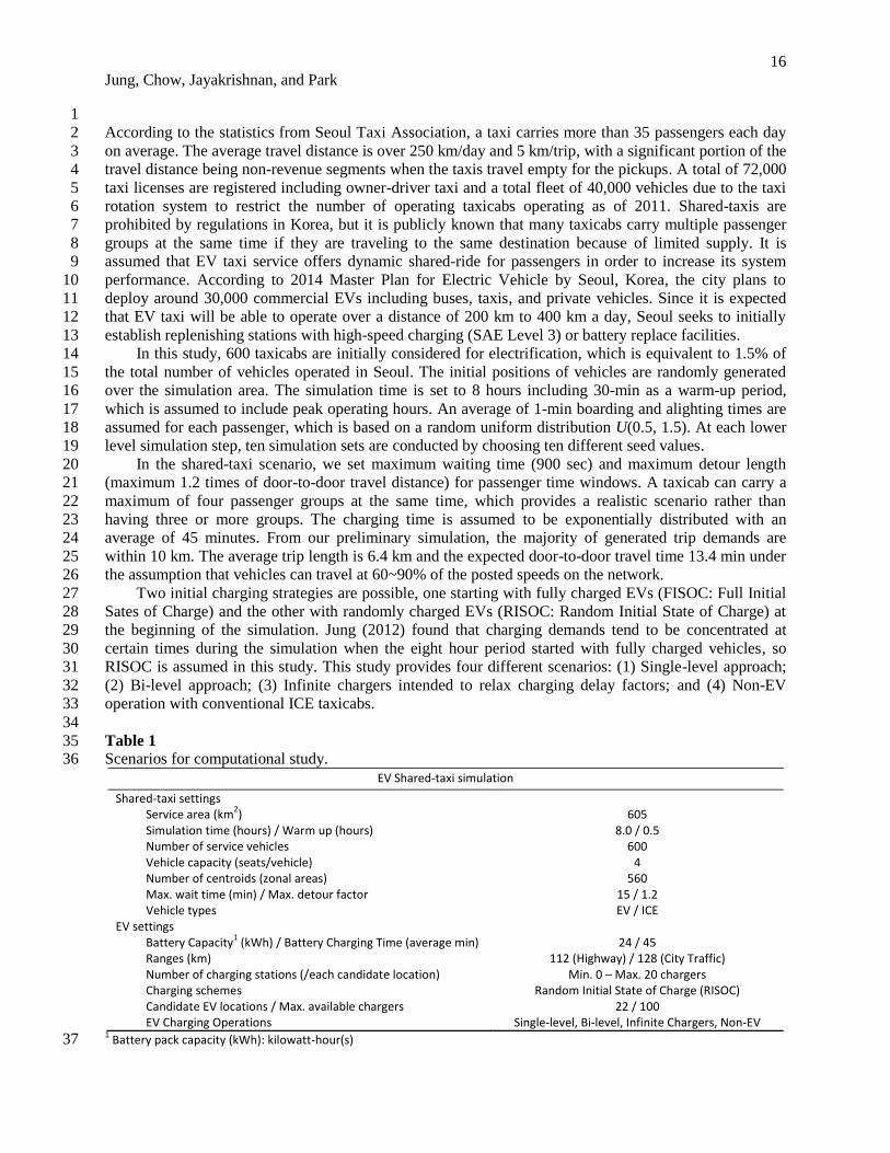
(b) Average queue delay and number of charging events 2

Fig. 6. Overall SDIRQ Performance by Bi-level Iterations. 3

4

When comparing the average queue delay and the number of charging events in Figure 6(b), the 5

proposed procedure not only decreases the average queue delay at charging locations, but also increases 6

the number of charging events at the same time. With the initial setting, each EV taxicab spends an 7

average queue delay of 3,730 sec/visit (62.2 min/visit) excluding battery replenishing time, which could 8

be a significant loss of service time when considering a vehicle might visit charging stations with an 9

average of 1.75 times during the 8-hour operation. As the iteration increases, the average queue delay 10

drops to 1,580 sec/visit (26.3 min/visit), which enables vehicles travel longer distance for its operation. 11

The average vehicle traveled distance increases from 130 km to 148.3 km as the procedure converges. In 12

other words, given the same size of fleet, the decreased queue delay at charging locations can improve the 13

EV fleet utilization, which causes more frequent charging behavior. 14

15

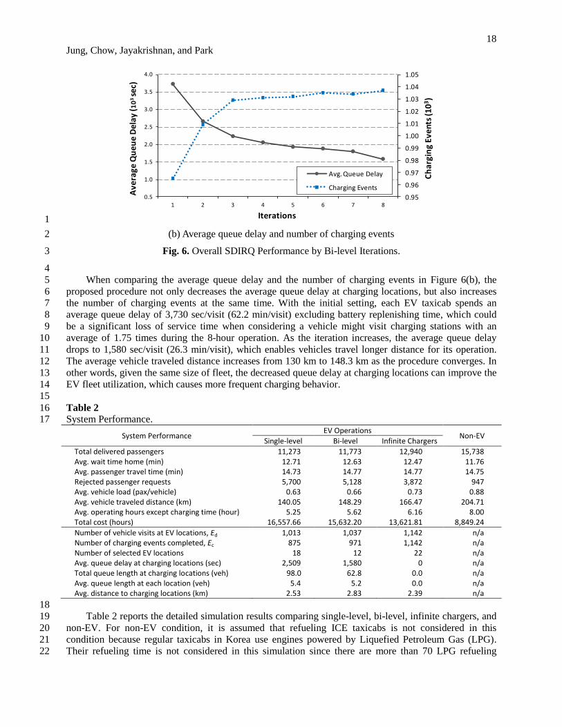
Table 2 16 System Performance. 17

System Performance EV Operations

Non-EV Single-level Bi-level Infinite Chargers

Total delivered passengers 11,273 11,773 12,940 15,738 Avg. wait time home (min) 12.71 12.63 12.47 11.76 Avg. passenger travel time (min) 14.73 14.77 14.77 14.75 Rejected passenger requests 5,700 5,128 3,872 947 Avg. vehicle load (pax/vehicle) 0.63 0.66 0.73 0.88 Avg. vehicle traveled distance (km) 140.05 148.29 166.47 204.71 Avg. operating hours except charging time (hour) Total cost (hours)

5.25 16,557.66

5.62 15,632.20

6.16 13,621.81

8.00 8,849.24

Number of vehicle visits at EV locations, Ed 1,013 1,037 1,142 n/a Number of charging events completed, Ec 875 971 1,142 n/a Number of selected EV locations 18 12 22 n/a Avg. queue delay at charging locations (sec) Total queue length at charging locations (veh)

2,509 98.0

1,580 62.8

0 0.0

n/a n/a

Avg. queue length at each location (veh) Avg. distance to charging locations (km)

5.4 2.53

5.2 2.83

0.0 2.39

n/a n/a

18

Table 2 reports the detailed simulation results comparing single-level, bi-level, infinite chargers, and 19

non-EV. For non-EV condition, it is assumed that refueling ICE taxicabs is not considered in this 20

condition because regular taxicabs in Korea use engines powered by Liquefied Petroleum Gas (LPG). 21

Their refueling time is not considered in this simulation since there are more than 70 LPG refueling 22

0.95

0.96

0.97

0.98

0.99

1.00

1.01

1.02

1.03

1.04

1.05

0.5

1.0

1.5

2.0

2.5

3.0

3.5

4.0

1 2 3 4 5 6 7 8

Ch

argi

ng

Eve

nts

(10

3)

Ave

rage

Qu

eu

e D

elay

(1

03

se

c)

Iterations

Avg. Queue Delay

Charging Events

19


locations in that area. Note that the non-EV condition causes additional financial and environmental costs 1

from EV taxi operations which are not considered in this study. 2

A higher average vehicle load indicates greater efficiency in taxi operation. Since the same vehicle 3

routing algorithm is applied to all scenarios, the average vehicle load gets worse as vehicles stay longer at 4

the charging locations. The single-level procedure ends up with a total of 18 locations selected for 5

allocating 100 chargers while the bi-level result shows 12 locations with the same total number of 6

chargers. A significant difference in the queue delays is measured between single-level and bi-level. The 7

single-level result reports an average 2,509 sec/visit (41.8 min/visit) of queue delay at each location, 8

which is about 15.5 min/visit more than the bi-level result. An average distance to charging location is 9

defined as a weighted distance by the number of charging events representing from a vehicle’s last 10

delivery position to the charging location where the vehicle is headed. If all candidate locations are used, 11

the average distance is 2.39 km. The bi-level result shows the 0.3 km higher distance due to the smaller 12

number of charging locations selected. Average actual taxi service hours with EV operations show less 13

than 77% of Non-EV even without queue delay impact. Single-level shows 5.25 hours of service 14

operation, which indicates average 2.75 hours are spent on moving to charging locations, queueing, and 15

refueling. 16

Figure 7 reports the distribution of EV chargers on the geographical area. The colored polygons 17

show the spatial distribution of increase in request rejection rate compared with non-EV scenario. The 18

thicker color means there is a greater increase in passenger pickup request rejections in a zone. The size 19

of circles represents the number of chargers allocated at each candidate location. The rejection rate 20

increases around the EV charger allocated areas are less than the other areas. For example, the zonal areas 21

around locations D, J, and Q show higher rejection rates in both Figure 7(a) and 7(b). This is because 22

vehicles would choose nearby pickup requests when they finish EV charging. The bi-level solution 23

clearly shows lower rejection rate than the single-level solution. Both solutions try to place more chargers 24

in the center of Seoul. The spatial distribution of chargers in Figure 7(b) shows a similar pattern in 25

comparison with the distribution of stochastic taxi demand in Figure 5(a). 26

27

20


1

2

(a) Single-level 3

4

(b) Bi-level 5

Fig. 7. Changes in Passenger Rejection Rate of EV Taxi Operation. 6

21


1

Figure 8 shows the comparison between the number of vehicle visits and the number of chargers 2

allocated at each location. The EV charger utilization (vehicle visits / charger) shows higher values with 3

the bi-level results. 4

5

6

(a) Single-level 7

8

(b) Bi-level 9

Fig. 8. EV Charger Allocation and Simulated Charging Demands. 10

11

Figure 9 provides a side-by-side comparison for average queue delay at charging locations and 12

average distance to charging locations. The average delays show significant difference between single-13

level and bi-level results. Locations such as C, G, K, L, and M in Figure 9(a) show lower average queue 14

delays with single-level, but they also show extremely higher queue delays at locations with a fewer 15

numbers of chargers. In contrast, the bi-level results show lower deviation in average queue delays on all 16

selected locations. Figure 9(b) reports the average distance to charging locations. Most of them remain 17

less than 3 km except the location D in single-level. These values can be used for re-calibration of the 18

critical battery level considered in the recharging scheme. Note that these distances to charging locations 19

0

20

40

60

80

100

120

140

160

0

2

4

6

8

10

12

14

16

18

20

A B C D E F G H I J K L M N O P Q R S T U V

Nu

mb

er

of

Ve

hic

le V

isit

s

EV

Ch

arg

ers

Candidate Locations

EV Chargers

Vehicle Visits

0

20

40

60

80

100

120

140

160

0

2

4

6

8

10

12

14

16

18

20


Nu

mb

er

of

Ve

hic

le V

isit

s

EV

Ch

arg

ers

Candidate Locations

EV Chargers

Vehicle Visits

22


are affected by the location distribution itself, in which vehicles tend to reject passengers whose 1

destinations are far from any of charging locations when the battery level gets critical. 2

3

4

(a) Average Queue Delay at Charging Locations 5

6

(b) Average Distance to Charging Locations 7

Fig. 9. Queue Delay at Locations and Average Distance to Charging Locations. 8

9

The temporal distribution of the aggregated EV charger occupancy and total queue length at 10

charging locations are provided in Figure 10. The warm-up time period is not included. As the simulation 11

starts, vehicles are visiting charging stations and saturate them after two hours in Figure 10(a). The bi-12

level solution shows an 8.2% higher occupancy level of EV chargers than the single-level. That indicates 13

higher utilization of charging system with the bi-level solution given the same refueling time. Once the 14

occupancy of chargers is saturated, the queue length starts decreasing in both solutions. Indeed, it is 15

conceivable that the charging demands of EV fleet operations are not constant, but the demand itself can 16

be influenced by the charging system performance. In other words, as charging locations hold more 17

vehicles for longer in the queue, the subsequent charging demands decrease as well as the system delivery 18

performance due to the changes in vehicle itinerary. This will be an important problem to be considered 19

when available chargers are not enough to support a deployed fleet size. 20

21

0

1

2

3

4

5

6

7

8


De

lay

(103

sec)

Candidate Locations

Single-level

Bi-Level

0

1

2

3

4

5

6


Avg

. Dis

tan

ce (k

m)

Candidate Locations

Single-level

Bi-level

23


1

2

(a) EV Charger Occupancy (chargers) 3

4

5

(b) Total Queue Length (vehicles) 6

Fig. 10. EV charger Occupancy and Total Queue Length at Charging Locations 7

8

Regarding the queue length, both solutions reach their maximums around 3:30, and then start 9

decreasing. The peak charging demand combined with the occupancy and the queue length is estimated 10

around up to 3:00 after warm-up. The queue length of the single-level solution keeps increasing after 5:00. 11

The overall average queue length of the single-level solution is 55% higher than the bi-level. Considering 12

the bi-level solution generates more charging events than the single-level, the EV charger distribution and 13

the location selection of the single-level is clearly worse than the bi-level solution. 14

Figure 11 compares the temporal relationship between the charging events generated and the 15

passenger pickup request rejections. The request rejection curves are aggregated every 5 min. As 16

mentioned, the peak charging demand is shown during the first three hours, and then the charging demand 17

decreases. The passenger request rejection peaks around 3:00, which is consistent with holding more 18

vehicles at charging locations as shown in Figure 10. The EV charging demands are derived from the taxi 19

operation caused by passenger requests. The spatial and temporal characteristics of charging demand can 20

be significantly influenced by the taxi demand, and neither of these characteristics can be analyzed using 21

node-based or flow-based model location models. 22

0

20

40

60

80

100

120

0:30 1:30 2:30 3:30 4:30 5:30 6:30 7:30

EV

Ch

arg

er

Occ

up

an

cy

Simulation Hours (00:30-08:00)

Bi-level Single-level

0

20

40

60

80

100

120

140

160

0:30 1:30 2:30 3:30 4:30 5:30 6:30 7:30

Qu

eu

e L

en

gth

(v

eh

icle

s)


Single-level Bi-level

24


1

2

(a) Single-level 3

4

(b) Bi-level 5

Fig. 11. Passenger Request Rejection and Charging Events 6

7

In summary, these results show that the proposed model is capable of locating charging stations with 8

stochastic dynamic itinerary-interception and queue delay. The proposed bi-level solution method 9

improves upon the benchmark algorithm without the interaction effects (allocation of fixed demand and 10

demand realization with fixed allocation, but no feedback mechanism) in terms of realized queue delay 11

(37%), total taxi service operating hours (6.7%), and reduced service request rejections (10%). 12

Furthermore, we show how much additional benefit in level of service (17.7%) can be achieved if the 13

current budget of 100 charging stations approaches infinity. 14

Obviously, having longer charging times will reduce the number of passengers served on average. 15

Compared to the non-EV scenario for the 600 shared-taxis, having infinite number of chargers (queueing 16

no longer becomes an issue), the reduction in number of delivered passengers is 17.8%. With only 100 17

charging stations, the number of delivered passengers is 25.2% of the non-EV scenario. These results, 18

along with the others presented in Table 2, give decision-makers trade-off values to consider in their 19

planning. For example, it is possible to evaluate the change in queue delay, allocation of charging stations, 20

and number of passengers served if the charging time can be technologically improved by 50%. It is also 21

possible to modify the simulation so to evaluate the presence of charging station queue informatics to the 22

central dispatch. Currently the simulation considers taxicabs going to the closest server node, but a more 23

0

5

10

15

20

25

30

35

40

45

50

0

10

20

30

40

50

60

70

80

90

100

0:30 1:30 2:30 3:30 4:30 5:30 6:30 7:30

Ch

argi

ng

Eve

nts

Re

qu

est

Re

ject

ion


Charging Events Request Rejection

0

5

10

15

20

25

30

35

40

45

50

0

10

20

30

40

50

60

70

80

90

100

0:30 1:30 2:30 3:30 4:30 5:30 6:30 7:30

Ch

argi

ng

Eve

nts

Re

qu

est

Re

ject

ion


Charging Events Request Rejection

25


efficient solution may be achieved if the dispatch is informed on average wait times at each node in real 1

time. The difference in objective value would be the value of investing in that information. These trade-2

off values will be crucial for justifying the research and development investments in the battery 3

technology, in equipping the charging stations and fleet with proper information flow, and in convincing 4

taxi companies to switch to electric vehicles. 5

6

5. CONCLUSION 7

Implementation of EV FTS has received growing attention from policy-makers because mobile 8

technologies make it easier to operate FTS and the clean energy technologies produce less GHG 9

emissions in urban areas. This study focuses on the EV facility location problem for EV taxi service with 10

FTS fleets in which vehicles operate with a stochastic dynamic itinerary. As opposed to the conventional 11

refueling station problems with node-based static charging demands, the proposed SDIRQ is a simulation 12

based bi-level optimization model in which EV refueling events are dynamically derived from the spatial 13

and temporal passenger demand levels. The lower-level problem involves an EV shared-taxi simulation 14

model to minimize both pickup requests and passenger travel times, while the upper-level objective offers 15

the optimal refueling locations and the allocation of chargers. 16

For the baseline comparison, a single-level approach is introduced by relaxing the charging 17

constraints to collect static charging demands in a conventional manner. Due to the complexity of 18

involving the queueing model in the objective functions, a bi-level solution approach is proposed. The 19

computational results report that SDIRQ with the bi-level approach shows a promising solution approach 20

given the demonstrated EV FTS. 21

It is worthwhile to mention the lack of spatial-equity in the proposed solution. For example, it only 22

takes into account the benefit distribution of EV locations and distributions for EV FTS operations. As 23

mentioned in the simulation results, customers in the zones that are far from the EV locations may have 24

lower chances to be served by EV taxicabs, in which case those customers are significantly worse off. On 25

the other hand, the customers near charging stations will have much higher chance to be picked up. This 26

might be a practical issue when determining the optimal EV charging facility locations. The spatial-equity 27

issue will be studied further. 28

Another area of future research is the integration of the loading on the power grid or incorporating 29

smart grid features, perhaps similar to He et al.’s (2013) study. Having an integrated approach can allow 30

scheduling both the charging location and time to minimize delay on the fleet and temporal loading 31

constraints on the grid. Time-of-day pricing should be considered in this case. 32

The location problem may also be viewed as a sequential, dynamic decision under uncertainty to 33

introduce flexibility to adapt the investment strategy over time, similar to the forecast horizon introduced 34

in the dynamic server relocation problem by Chow and Regan (2011). The recent work by Chung and 35

Kwon (2012) shows a promising effort in that direction, introducing a multi-period aspect to the refueling 36

location problem, although demand is kept deterministic. 37

38

ACKNOWLEDGMENTS 39

Dr. Jung and Dr. Jayakrishnan were funded by the Korea Transport Institute (KOTI), as part of “2011 40

Electric Vehicle Research on Business”, initiated by the National Research Council for Economics, 41

Humanities and Social Science, South Korea. Dr. Chow was partially supported by funding from the 42

Canada Research Chairs program. 43

26


REFERENCES 1

[1] Alshalalfah, B., Shalaby, A., 2012. Feasibility of flex-route as a feeder transit service to rail 2

stations in the suburbs: case study in Toronto. Journal of Urban Planning and Development 138(1), 3

90-100. 4

[2] Asiaone.com, “Taxi-sharing app to launch here end June”, June 8, 2012, 5

http://www.asiaone.com/Motoring/News/Story/A1Story20120608-351278.html, accessed April 15, 6

2013. 7

[3] Barth, M., Todd, M., 2001. User behavior evaluation of an intelligent shared electric vehicle 8

system. Transportation Research Record 1760, 145-152. 9

[4] Berman, O., Larson, R.C., Fouska, N., 1992. Optimal location of discretionary service facilities. 10

Transportation Science 26(3), 201-211. 11

[5] Berman, O., Krass, D., Xu, C.W., 1995. Locating discretionary service facilities based on 12

probabilistic customer flows. Transportation Science 29(3), 276-290. 13

[6] Berman, O., Drezner, Z., 2007. The multiple server location problem. The Journal of the 14

Operational Research Society 58(1), 91-99. 15

[7] Better Place, Tokyo Electric Taxi Project Overview. http://www.betterplace.com/global/progress. 16

Accessed March 02, 2012. 17

[8] Boyaci, B., Geroliminis, N., 2011. Extended hypercube models for large scale spatial queueing 18

systems. STRC 2011, 19p. 19

[9] Capar, I., Kuby, M., 2012. An efficient formulation of the flow refueling location model for 20

alternative-fuel stations. IIE Transactions 44(8), 622-636. 21

[10] Cervero, R. Paratransit in America: Redefining Mass Transportation. Praeger Publishers, Westport, 22

Conn., 1997. 23

[11] Cheng, R. and Gen, M. Evolution program for resource constrained project scheduling problem. 24

Evolutionary Computation in IEEE World Congress, pp. 736-741, 1994. 25

[12] China.org.cn, 2012. “Beijing promotes taxi sharing to ease traffic jams”. 26

http://www.china.org.cn/video/2012-03/31/content_25040109.htm, accessed March 29, 2013. 27

[13] Chow, J.Y.J., Regan, A.C., 2011. Resource location and relocation models with rolling horizon 28

forecasting for wildland fire planning. INFOR 49(1), 31-43. 29

[14] Chung, S.H., Kwon, C., 2012. Multi-period planning for electric-car charging station locations: a 30

case of Korean expressways. Working paper, 31p., http://infohost.nmt.edu/~schung/chung2012.pdf. 31

[15] Church, R., ReVelle, C., 1974. Maximal covering location problem. Papers in Regional Science 32

32(1), 101–118. 33

[16] Cortés, C.E., Jayakrishnan, R., 2002. Design and operational concepts of high-coverage point-to-34

point transit system. Transportation Research Record 1783, 178-187. 35

[17] Crainic, T.G., Errico, F., Malucelli, F., Nonato, M., 2012. Designing the master schedule for 36

demand-adaptive transit systems. Annals of Operations Research 194(1), 151-166. 37

[18] Dial, R. B., 1995. Autonomous dial-a-ride transit introductory overview. Transportation Research 38

3C(5), 261-275. 39

[19] Drezner, Z., Hamacker, H. (eds), 2002. Facility Location: Applications and Theory, Springer, New 40

York. 41

[20] eGlobal Travel Media, 2011. “Seoul unveils ‘2014 Master Plan for Electric Vehicle’”. 42

http://www.eglobaltravelmedia.com.au/destinations/seoul-unveils-%E2%80%9C2014-master-plan-43

for-electric-vehicle%E2%80%9D.html, accessed March 24, 2013. 44

[21] FedEx. FedEx Cleaner Vehicles. http://about.van.fedex.com/article/cleaner-vehicles. Accessed 45

March 20, 2012. 46

[22] Hadas, Y., Ceder, A., 2008. Multiagent approach for public transit system based on flexible routes. 47

Transportation Research Record 2063, 89-96. 48

[23] He, F., Wu, D., Yin, Y., Guan, Y., 2013. Optimal deployment of public charging stations for plug-49

in hybrid electric vehicles. Transportation Research Part B 47, 87-101. 50

http://www.asiaone.com/Motoring/News/Story/A1Story20120608-351278.html

http://www.china.org.cn/video/2012-03/31/content_25040109.htm

http://infohost.nmt.edu/~schung/chung2012.pdf

http://www.eglobaltravelmedia.com.au/destinations/seoul-unveils-%E2%80%9C2014-master-plan-for-electric-vehicle%E2%80%9D.html

http://www.eglobaltravelmedia.com.au/destinations/seoul-unveils-%E2%80%9C2014-master-plan-for-electric-vehicle%E2%80%9D.html

27


[24] Hodgson, M.J., 1990. A flow-capturing location-allocation model. Geographical Analysis 22(3), 1

270-279. 2

[25] Iglehart, D.L., 1965. Limiting diffusion approximations for the many server queue and the 3

repairman problem. Journal of Applied Probability 2(2), 429-441. 4

[26] Jiang, Y., Zhang, Y., Zhang, C., Fan, J., 2012. The capacitated deviation-flow fueling location 5

model for siting battery charging stations. In: Proc. CICTP 2012, ASCE, 2771-2778. 6

[27] Jung, J., 2012. Shared-ride passenger transportation systems with real-time routing. PhD 7

Dissertation, University of California, Irvine, 186 pp. 8

[28] Jung, J., Jayakrishnan, R., 2012. High-coverage point-to-point transit: electric vehicle operations. 9

Transportation Research Record 2287, 44-53. 10

[29] Jung, J., Jayakrishnan, R., Park, J.Y., 2013. Design and modeling of real-time shared-taxi dispatch 11

algorithms. In: Proc. 92nd TRB Annual Meeting, Washington, DC. 12

[30] Jung, J., Jayakrishnan, R., Choi, K., 2013.Shared-Taxi Operations with Electric Vehicles. Working 13

paper, UCI-ITS-WP-13-1, University of California, Irvine, 22p., 14

http://www.its.uci.edu/its/publications/papers/ITS/UCI-ITS-WP-13-1.pdf 15

[31] Kameda, H., Mukai, N., 2011. Optimization of charging station placement by using taxi probe data 16

for on-demand electrical bus system. In: Proc. KES 2011, Part III, LNAI 6883, 606-615. 17

[32] Kang, J.E., Recker, W.W., 2012. Strategic hydrogen refueling station locations with scheduling and 18

routing considerations of individual vehicles. Working paper, UCI-ITS-WP-12-2, University of 19

California, Irvine, 37p., http://www.its.uci.edu/its/publications/papers/ITS/UCI-ITS-WP-12-2.pdf 20

[33] Kang, J.E., Chow, J.Y.J., Recker, W.W., 2013. On activity-based network design problems. 21

Transportation Research Part B, Special Issue on ISTTT 20, in press, doi: 22

10.1016/j.trb.2013.05.009. 23

[34] Kim, M., Schonfeld, P., 2012. Conventional, flexible, and variable-type bus services. Journal of 24

Transportation Engineering 138(3), 263-273. 25

[35] Kim, J.G., Kuby, M., 2012. The deviation-flow refueling location model for optimizing a network 26

of refueling stations. International Journal of Hydrogen Energy 37(6), 5406-5420. 27

[36] Kimura, T., 1983. Diffusion approximation for an M/G/m queue. Operations Research 31(2), 304-28

321. 29

[37] Koffman, D., 2004. TCRP Synthesis 53: Operational Experiences with Flexible Transit Services, 30

Transit Cooperative Research Program, Transportation Research Board, Washington, DC, 71p. 31

[38] Kuby, M., Lim, S., 2005. The flow-refueling location problem for alternative-fuel vehicles. Socio-32

Economic Planning Sciences 39(2), 125-145. 33

[39] Kuby, M., Lim, S., 2007. Location of alternative-fuel stations using the flow-refueling location 34

model and dispersion of candidate sites on arcs. Networks and Spatial Economics 7(2), 129-152. 35

[40] Laporte, G., Nobert, Y., Taillefer, S., 1988. Solving a family of multi-depot vehicle routing and 36

location-routing problems. Transportation Science 22(3), 161-172. 37

[41] Larson, R., 1974. A hypercube queueing model for facility location and redistricting in urban 38

emergency services. Computers & Operations Research 1(1), 67-95. 39

[42] Lau, J. K. S., Tham, C. K., & Luo, T. (2011). Participatory cyber physical system in public 40

transport application. 4th IEEE International Conference on Utility and Cloud Computing, 355-360. 41

[43] Lin, Z., Ogden, J., Fan, Y., Chen, C.W., 2008. The fuel-travel-back approach to hydrogen station 42

siting. International Journal of Hydrogen Energy 33(12), 3096-3101. 43

[44] Lovell, D.J., Vlachou, K., Rabbani, T., Bayen, A., 2012. A diffusion approximation to a single 44

airport queue. Transportation Research Part C, in press, doi: 10.1016/j.trc.2012.04.010. 45

[45] Mak, H.Y., Rong, Y., Shen, Z.J.M., 2012. Infrastructure planning for electric vehicles with battery 46

swapping. Working paper, http://ssrn.com/abstract=2022651. 47

[46] Marianov, V., ReVelle, C., 1996. The queueing maximal availability location problem: a model for 48

the siting of emergency vehicles. European Journal of Operational Research 93(1), 110-120. 49

[47] Marianov, V., Serra, D., 1998. Probabilistic, maximal covering location-allocation models for 50

congested systems. Journal of Regional Science 38(3), 401-424. 51

http://www.its.uci.edu/its/publications/papers/ITS/UCI-ITS-WP-13-1.pdf

http://www.its.uci.edu/its/publications/papers/ITS/UCI-ITS-WP-12-2.pdf

http://ssrn.com/abstract=2022651

28


[48] MirHassani, S.A., Ebrazi, R., 2012. A flexible reformulation of the refueling station location 1

problem. Transportation Science, in press, doi: 10.1287/trsc.1120.0430. 2

[49] Mulley, C., Nelson, J.D., 2009. Flexible transport services: a new market opportunity for public 3

transport. Research in Transportation Economics 25(1), 39-45. 4

[50] Nourbakhsh, S.M., Ouyang, Y., 2010. Optimal fueling strategies for locomotive fleets in railroad 5

networks. Transportation Research Part B 44(8-9), 1104-1114. 6

[51] Nourbakhsh, S.M., Ouyang, Y., 2012. A structured flexible transit system for low demand areas. 7

Transportation Research Part B 46(1), 204-216. 8

[52] Owen, S.H., Daskin, M.S., 1998. Strategic facility location: a review. European Journal of 9

Operational Research 111(3), 423–447. 10

[53] Pasternack, B.A., Drezner, Z., 1998. A note on calculating steady state results for an M/M/k 11

queueing system when the ratio of the arrival rate to the service rate is large. Journal of Applied 12

Mathematics & Decision Sciences 2(2), 201-203. 13

[54] Perl, J., Daskin, M.S., 1985. A warehouse location-routing problem. Transportation Research, 14

19B(5), 381-396. 15

[55] Quadrifoglio, L., Li, X., 2009. A methodology to derive the critical demand density for designing 16

and operating feeder transit services. Transportation Research Part B 43(10), 922-935. 17

[56] Recker, W.W. (1995). The household activity pattern problem: general formulation and solution. 18

Transportation Research 29B(1), 61-77. 19

[57] Rolfe, A.J., 1971. A note on marginal allocation in multiple-server service systems. Management 20

Science 17(9), 656-658. 21

[58] Snyder, L., 2006. Facility location under uncertainty: a review. IIE Transactions 38(7), 547–564. 22

[59] Stone, J. R., Nalevanko, A., Tsai, J., 1993. Assessment of software for computerized paratransit 23

operations. Transportation Research Record 1378, 1-9. 24

[60] Tao, C.C., 2007. Dynamic taxi-sharing service using intelligent transportation system technologies. 25

International Conference on Wireless Communications, Networking and Mobile Computing. Sept. 26

2007, 3209-3212. 27

[61] Tong, H.Y., Hung, W.T., Cheung, C.S., 2000. On-road motor vehicle emissions and fuel 28

consumption in urban driving conditions. Journal of the Air & Waste Management Association 29

50(4), 543-554. 30

[62] Tsukada, N., Takada, K., 2005. Possibilities of the large-taxi dial-a-ride transit system utilizing 31

GPS-AVM. Journal of Eastern Asia Society for Transportation Studies, EASTS, Bangkok, 32

Thailand, 1-10. 33

[63] Upchurch, C., Kuby, M., Lim, S., 2009. A model for location of capacitated alternative-fuel 34

stations. Geographical Analysis 41(1), 85-106. 35

[64] Upchurch, C., Kuby, M., 2010. Comparing the p-median and flow-refueling models for locating 36

alternative-fuel stations. Journal of Transport Geography 18(6), 750-758. 37

[65] U.S. Environmental Protection Agency (2006). Greenhouse Gas Emissions from the U.S. 38

Transportation Sector: 1990-2003. http://www.epa.gov/otaq/climate/420r06003.pdf. 39

[66] Wang, Y.W., Lin, C.C., 2009. Locating road-vehicle refueling stations. Transportation Research 40

Part E 45(5), 821-829. 41

[67] Wang, Y.W., Wang, C.R., 2010. Locating passenger vehicle refueling stations. Transportation 42

Research Part E 46(5), 791-801. 43

[68] Xi, X., Sioshansi, R., Marano, V., 2013. Simulation-optimization model for location of a public 44

electric charging infrastructure. Transportation Research Part D 22, 60-69. 45

[69] Zhao, J., Dessouky, M., 2008. Service capacity design problems for mobility allowance shuttle 46

transit systems. Transportation Research Part B 42(2), 135-146. 47

48

49

http://www.epa.gov/otaq/climate/420r06003.pdf

stochastic dynamic itinerary interception refueling ... · 6 stochastic dynamic itinerary...

Documents