Stochastic Growth Model

Prof. Lutz Hendricks

Econ720

December 5, 2018

1 / 40

Introduction

We now return to the stochastic growth model.We study

I the planner’s problemI the competitive equilibrium

Then we introduce heterogeneity and risk sharing.

2 / 40

Planning solution

The history of shocks is θ t.Preferences:

∞

∑t=0

βt∑θ t

Pr (θt|θ0)u(c [θ t]) (1)

Technology:

X = F (K,L,θ) + (1−δ )K− c (2)K′ = X (3)

3 / 40

Bellman equation

Define k = K/L.

V (k,θ) = maxk′∈[0,f (k,θ)+(1−δ)k]

u(f (k,θ) + (1−δ )k− k′

)(4)

+βE[V(k′,θ ′

)|θ]

(5)

4 / 40

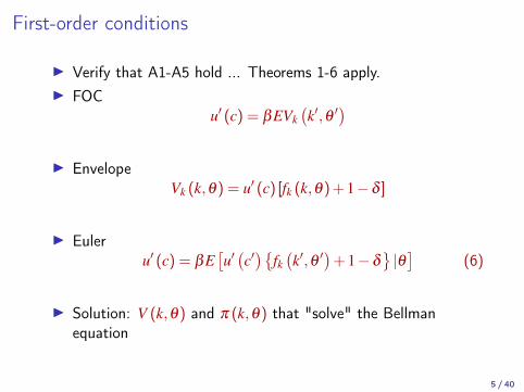
First-order conditions

I Verify that A1-A5 hold ... Theorems 1-6 apply.I FOC

u′ (c) = βEVk(k′,θ ′

)I Envelope

Vk (k,θ) = u′ (c) [fk (k,θ) + 1−δ ]

I Euleru′ (c) = βE

[u′(c′){

fk(k′,θ ′

)+ 1−δ

}|θ]

(6)

I Solution: V (k,θ) and π (k,θ) that "solve" the Bellmanequation

5 / 40

Characterization

I Now for the bad news ... there really isn’t much one can sayabout the solution analytically.

I But see Campbell (1994) for a discussion of a log-linearapproximation.

6 / 40

Competitive Equilibrium

Competitive equilibrium

The model comes in 2 flavors.

1. Complete marketsI for every history, there exists an asset that pays in that state of

the worldI the implication is complete risk sharing: all idiosyncratic risks

are insuredI aggregate risks remain

2. Incomplete marketsI some securities are missingI there is no representative agent

8 / 40

Trading arrangements

I With complete markets, date 1 Arrow-Debreu trading isconvenientI Uncertainty essentially disappears from the model.

I With incomplete markets, it is easiest to specify the set ofsecurities available at each date.I Sequential trading.

9 / 40

Complete markets - Arrow Debreu trading

I The environment is standard.I The history is of shocks is θ t.I Trading takes place at date 1.I The point: This looks like a static model without uncertainty.

10 / 40

Market arrangements

Goods markets: standard

I buy and sell consumption at each node θ t

I price p(θ t)

Labor markets: standard

I wage w(θ t)

Capital rental:

I households can buy goods in θ t and give them to firmsI firms then pay R

(θ t+1

)tomorrow

I this includes returning the undepreciated capital

11 / 40

Household: budget constraint

Expenditures in state θ t:

x(θt) = p(θ

t) [c(θt) + s(θ

t)] (7)

p(θ t) is the price of the good in state θ t.c is consumptions is "saving:" buy goods (capital) and rent to firms.

12 / 40

Household: budget constraint

Income in state θ t:

y(θt) = w(θ

t) + R(θt)s(θ

t−1) (8)

w(θ t) is the wage.R(θ t) is the payoff from renting a unit of the good to the firm.Both are state contingent.

Poor notation: keep in mind that θ t follows θ t−1

13 / 40

Household: budget constraint

Lifetime budget constraint:

∞

∑t=0

∑θ t

[y(θt)− x(θ

t)] + p(θ0)s0 = 0 (9)

s0 is the initial endowment of goods.

With Arrow-Debreu trading, there is a lifetime budget constraint,even under uncertainty.

I Because there really is no uncertainty any more.I At each node, the household’s spending and income are fully

predictable.

14 / 40

Firms

Firms maximize the total value of profits.

I There is no discounting because of Arrow-Debreu trading.

Profits in state θ t:

p(θt) [F (K [θ t] ,L [θ t] ,θt) + (1−δ )K [θ t]]

−R(θt)K (θ

t)−w(θt)L(θ

t)

Value of the firm: sum of profits over all states.

FOCs are standard:

I since the firm does not own anything, it maximizes profitsstate-by-state.

15 / 40

Competitive Equilibrium

I Allocation: c(θ t) ,s(θ t) ,K (θ t) ,L(θ t).I Price system: p(θ t) ,w(θ t) ,R(θ t) for all histories θ t.I These satisfy:

1. Household optimality.2. Firm optimality.3. Market clearing:

I L(θ t) = 1.I K (θ t,θt+1) = s(θ t).I Goods market.

16 / 40

Competitive EquilibriumComments

I This looks like a static model without uncertainty.I Each history defines new goods: output, labor, capital rental.

I The setup is far more complicated than the recursive one.

17 / 40

Risk Sharing

I What if agents are heterogeneous?I With complete markets, risk is perfectly shared.I The simplest case: An endowment economy with

Arrow-Debreu trading.I The state is θ t.

18 / 40

Risk SharingHouseholds

I There are I types of households, indexed by i.I Endowments are yi (θ t).I Preferences are

∑t

∑θ t

βtq(θ

t)ui (ci [θ t])

I Budget constraints:

∑t

∑θ t

p(θt)[ci (θ

t)− yi (θt)]

= 0 (10)

19 / 40

Risk SharingHouseholds

First-order conditions are as usual:

q(θt)β

t ∂ui(ci [θ t]

)∂ci [θ t]

= λip(θt) (11)

where λi is the Lagrange multiplier.

20 / 40

Risk Sharing

Complete risk sharing: For all θ t the MRS is equated acrosshouseholds:

MRS(

θt, θ̂ τ

)=−

β t ∂ui(ci [θ t]

)/∂ci [θ t]

β τ ∂ui(

ci[θ̂ τ

])/∂ci

[θ̂ τ

] =p(θ t)/q(θ t)

p(

θ̂ τ

)/q(

θ̂ τ

)Equivalently, the ratio of marginal utilities between 2 agents is thesame for all θ t:

∂ui(ci [θ t]

)/∂ci [θ t]

∂uj (ci [θ t])/∂cj [θ t]=

λi

λj(12)

21 / 40

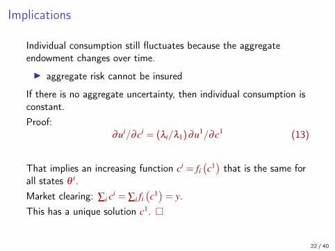
Implications

Individual consumption still fluctuates because the aggregateendowment changes over time.

I aggregate risk cannot be insured

If there is no aggregate uncertainty, then individual consumption isconstant.Proof:

∂ui/∂ci = (λi/λ1)∂u1/∂c1 (13)

That implies an increasing function ci = fi(c1)that is the same for

all states θ t.Market clearing: ∑i ci = ∑i fi

(c1)

= y.This has a unique solution c1. �

22 / 40

Sequential Trading

Sequential Trading

I We set up the C.E. with sequential trading.I If we want complete markets, we need Arrow securities.I Each security, a

(θ t+1

)is indexed by the state of the world in

which it pays off: θ t+1.I The asset is purchased for price p̄(θ t,θ ′) in state θ t.I It pays one unit of consumption if θ t+1 = [θ t,θ ′].

24 / 40

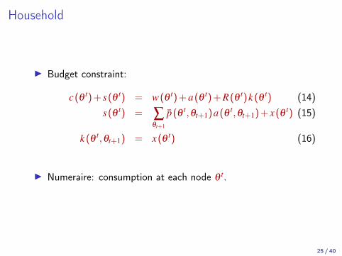
Household

I Budget constraint:

c(θt) + s(θ

t) = w(θt) + a(θ

t) + R(θt)k (θ

t) (14)s(θ

t) = ∑θt+1

p̄(θt,θt+1)a(θ

t,θt+1) + x(θt) (15)

k (θt,θt+1) = x(θ

t) (16)

I Numeraire: consumption at each node θ t.

25 / 40

Household

I Household problem:

max∞

∑t=0

βt∑θ t

Pr (θt|θ0)u(c [θ t]) (17)

s.t. budget constraints for all θ t.

26 / 40

Recursive household problem

I State: (−→a ,k,θ).I −→a : holdings of all the a(θ).

I Given prices: w and p̄(θ ,θ ′).I Bellman equation:

V (−→a ,k,θ) = maxc,a′(θ ′),k′

u(c) + β ∑θ ′

q(θ′|θ)

V(−→a ′,k′,θ ′)

s.t. budget constraint

∑θ ′

p̄(θ ,θ ′

)a′(θ′)+ k′+ c = w + a(θ) + Rk

27 / 40

First order conditions

I For a′ (θ ′):

u′ (c) p̄(θ ,θ ′

)= βq

(θ′|θ) ∂V (−→a ′ [θ ′] ,k′,θ ′)

∂a(θ ′)(18)

I For k′:

u′ (c) = β ∑θ ′

q(θ′|θ) ∂V (−→a ′,k′,θ ′)

∂k′(19)

28 / 40

First order conditionsI Envelope:

∂V (−→a ,k,θ)/∂a(θ) = u′ (c) (20)

∂V(−→a ,k, θ̂

)/∂a(θ) = 0 (21)

∂V (−→a ,k,θ)/∂k = u′ (c)R (22)

I Euler equation holds state by state for state contingent claims:

u′ (c) p̄(θ ,θ ′

)= βq

(θ′|θ)

u′(c[a′(θ′) ,θ ′]) (23)

I Euler equation for capital:

u′ (c) = β ∑θ ′

q(θ′|θ)

R(θ ,θ ′

)u′(c[a′(θ′) ,k′,θ ′]) (24)

= βE R′ u′(c′)

29 / 40

No arbitrage

I Since capital can be replicated by buying a set of Arrowsecurities:

∑θ ′

p̄(θ ,θ ′

)R(θ ,θ ′

)= 1 (25)

I Proof: Solve (23) for q(θ ′|θ) and substitute into (24).

30 / 40

Equilibrium

I We can write down a sequential equilibrium definition, similarto the Arrow-Debreu.I Everything is indexed by θ t.

I More powerful: Recursive Competitive Equilibrium.I Everything is a function of the current state.

31 / 40

Recursive CE

I Define an aggregate state vector: S = (θ ,K).I In general: we need to keep track of the distribution of (θi,ki)

across households.I Here: all households are identical.

I The law of motion for the aggregate state:

Pr(θ′|θ)

= q(θ′|θ)

K′ = G(θ ,K)

where G is endogenous.

32 / 40

Recursive CEHousehold

I Given:I aggregate state and its law of motion.I price functions: w(S) ,R(S) and p̄(S,θ ′).

I Bellman equation:

V (−→a ,k,S) = maxc,a′(θ ′),k′

u(c) + β ∑θ ′

q(θ′|θ)

V(−→a ′ [θ ′] ,k′,S′)

s.t. budget constraint

∑θ ′

p̄(θ ,θ ′

)a′(θ′)+ k′+ c = w(S) + a(θ) + R(S)k

and aggregate law of motion

S′ = G(S)

33 / 40

Recursive CE

I First-order conditions: unchanged.I Solution: V (a,k,S) and policy functions c(a,k,S),

k′ = κ (a,k,S).

34 / 40

Recursive CEFirm

I Always the same because the firm has a static problem:I Solution: R(S) ,w(S).

35 / 40

Recursive CE

I Equilibrium objects:

1. Household: Value function and policy functions.2. Firm: Price functions.3. Aggregate law of motion: K′ = G(θ ,K).

I Equilibrium conditions:

1. Household optimality.2. Firm optimality.3. Market clearing.4. Consistency:

G(θ ,K) = κ (K,θ ,K) (26)

where the household’s policy function is k′ = κ(k,θ ,K).

36 / 40

Recursive CE

I Note: We could toss out all the Arrow securities withoutchanging anything.

I The model boils down to:

1. Euler equation for K: u′ (c) = βE [R′u′ (c′)]2. Law of motion for K: K′ = F (K,L) + (1−δ )K− c.3. FOC: R = FK (K,L) + 1−δ .

I This changes when individuals are not identical.

37 / 40

Recursive CEWhat do we gain?

I Avoid having to carry around infinite histories.I Equilibrium contains few objects.

I Especially when the economy is stationary.

I All endogenous objects are functions.I Results from functional analysis can be used to determine their

properties.

I Recursive CE is easy to compute.

38 / 40

Reading

I Acemoglu (2009) ch. 16-17.I Krusell (2014) ch. 6I Stokey et al. (1989) discuss the technical details of stochastic

Dynamic Programming.I Ljungqvist and Sargent (2004), ch. 2 talk about Markov

chains. Ch. 7 covers complete market economies(Arrow-Debreu and sequential trading). Ch. 6: Recursive CE.

I Campbell (1994) discusses an analytical solution (approximate)

39 / 40

References I

Acemoglu, D. (2009): Introduction to modern economic growth,MIT Press.

Campbell, J. Y. (1994): “Inspecting the mechanism: An analyticalapproach to the stochastic growth model,” Journal of MonetaryEconomics, 33, 463–506.

Krusell, P. (2014): “Real Macroeconomic Theory,” Unpublished.

Ljungqvist, L. and T. J. Sargent (2004): Recursive macroeconomictheory, 2nd ed.

Stokey, N., R. Lucas, and E. C. Prescott (1989): “RecursiveMethods in Economic Dynamics,” .

40 / 40