Stochastic modelling of catastrophe risks in internal models

Dr. Dorothea Diers

Provinzial NordWest Holding AG, Münster, Germany

1

Zusammenfassung

Die Messung und Bewertung von Katastrophenrisiken stellt sich als sehr bedeutsa-

mes Gebiet dar, da sie einen großen Teil des gesamten Risikokapitals der Unter-

nehmen binden. Aus diesem Grund soll der vorliegende Aufsatz zwei konkrete An-

sätze zur Modellierung von Katastrophenschäden am Beispiel der Sturmereignisse

vergleichend darstellen, die beide Ergebnisse aus Naturgefahrenmodellen verwen-

den. Während das erste Verfahren komplette Event Loss Tables verarbeitet, nutzt

der zweite mathematisch-statistische Ansatz Informationen über bestimmte Wieder-

kehrperioden. Die beiden Methoden werden anhand von Beispieldaten verglichen

und deren Vor- und Nachteile bei der Anwendung im Steuerungskontext aufgezeigt.

Schlussendlich werden Risikokapitalien berechnet und die Wirkung von Strategien

auf den Risikokapitalbedarf getestet.

Schlagwörter: Interne Modelle, Katastrophenrisiken, Naturgefahrenmodelle, Event

Loss Tables, Risikokapital, Wert- und Risikoorientierte Unternehmenssteuerung

Abstract

Measuring and evaluating catastrophe risk has come to be a very important issue, as

a substantial share of the company’s entire risk capital is committed to natural ca-

tastrophes. The following study aims to present two actual approaches in modelling

loss due to natural catastrophes taking storms as an example. Both models use re-

sults from natural risks models. The first method is based on processing complete

event loss tables, while the second mathematical statistical approach uses informati-

on from certain return periods. Both methods will be compared using example data,

and their advantages and disadvantages will be pointed out as applicable to value

and risk-based management. Finally, the study tests the impact of strategies on risk

capital requirement.

Keywords: Internal models, catastrophe risk, natural risk models, event loss tables,

risk capital, value and risk-based management

2

Stochastic modelling of catastrophe risks in internal models

Dorothea Diers*

1 INTRODUCTION........................................................................................................... 2

2 CATASTROPHE CLAIMS IN INTERNAL MODELS............................................... 4

3 APPROACHES FOR CATASTROPHE RISK MODELLING .................................. 7

3.1 APPROACH BASED ON NATURAL RISK MODELS ............................................................ 7

3.2 MATHEMATICAL STATISTICAL APPROACHES ............................................................. 13

3.3 COMPARISON OF THE TWO MODELLING APPROACHES................................................ 21

4 IMPACT OF THE TWO MODELLING APPROACHES ON RISK CAPITAL

REQUIREMENT ................................................................................................................... 22

5 CONCLUSION AND OUTLOOK ............................................................................... 24

1 Introduction

Negative developments on the capital markets at the beginning of the millennium

along with the increase in natural catastrophes and terrorist attacks have substan-

tially altered the risk situation facing the insurance industry. As an example, total cor-

porate capital resources decreased by around between 25% from 2000 to 2002 in

non-life insurance and reinsurance across the world according to SWISS RE.1 Insur-

ance companies have reacted to the altered prevailing conditions with modern man-

agement techniques such as value and risk-based management.

This involves measuring success at reaching a risk adjusted return on the risk capital

provided by the investors. The risk capital should be derived from the actual risks

* Provinzial NordWest Holding AG, Münster, Germany, dorothea.diers@provinzial.de. We are grateful to the unknown referee of GRIR and the participants of the ASTIN meeting 2008 (Manchester) for valuable sugges-tions and comments on an earlier draft of this paper. 1 See [Swiss Re 2002].

3

facing the company. Companies will only be able to assess the level of risk capital

and the complete distribution of results according to their individual risk structure with

the help of high-quality internal models (DFA models)2 matched as closely as possi-

ble to the risk situation they aim to represent, thus addressing issues as to risk-

bearing ability and profitability of the company as a whole as well as in different lines

of business.

Adequately assessing the risk situation of a company involves appropriately repre-

senting the individual risks that the company is exposed to in DFA models. Modelling

catastrophe events plays a major role in this matter, as natural catastrophes often

involve considerable loss potential that the company’s risk management must take

into account sufficiently. A considerable share of risk capital is often committed to

insurance divisions affected by catastrophe events, which is why risks of natural ca-

tastrophes have a major impact on selecting a suitable reinsurance policy. This

should lead to intensive discussion with reinsurance departments on the adequate

level of reinsurance protection with regard to risk and return. The matter is made

worse by the brief experience in catastrophe events – the small number of observa-

tions in the history – amongst most insurance companies, while long return periods

such as a hundred, five hundred, thousand or ten thousand-year events pose a great

challenge to adequate modelling for most companies.

Catastrophe claims refer to loss caused by any single event affecting a large number

of insured policies within the same time frame. The following natural catastrophes

play an especially important role:

• Storms,

• Earthquakes,

• Hailstorms,

• Floods.

This study aims to provide a quantitative analysis for two different approaches in ca-

tastrophe modelling taking storms as an example, with reference to model data.3

2 Interested readers will find an actual proposal for the development of a stochastic internal model (DFA model: dynamic financial analysis) useful as a basis for value and risk-based management in Diers, D. (2007a). The necessary steps from initial concept to complete preparation and implementation are presented here. The indi-vidual modelling approaches are shown with reference to data from a model company. 3 The remaining storm losses may be modelled as attritional losses that are far less volatile.

4

Both approaches use results from natural risks models. The first method is based on

processing complete event loss tables, while the second mathematical statistical ap-

proach uses information from certain return periods. Both methods will be compared

using example data, and their advantages and disadvantages will be pointed out as

applicable to value and risk-based management. Finally, the study tests the impact of

strategies on risk capital requirement.

2 Catastrophe claims in internal models

DFA models are aimed at covering the broadest possible range of all possible profit

and loss accounts in the next year, or years in models covering several years, in or-

der to represent the risk situation of the company adequately and determine the indi-

cators relevant to corporate strategy, such as expected company results and risk

capital. However, insurance-related risks in non-life insurance are subject to serious

variability resulting from the high level of volatility by both claim severity and fre-

quency.4 As an example, storms may lead to extremely high total claims due to an

enormous number of more minor claims. This is why both claim and capital market

development should be stochastically modelled. To this end, a DFA model should be

understood as a simulation model. Analytical models are unsuitable for non-life in-

surance, as the total results distribution can only be determined by very restrictive

assumptions.5

Two main aspects need to be considered modelling catastrophe claims. On the one

hand, the basic assumptions of the collective model – which are usually valid in the

case of non-catastrophe modelling concerning attritional and large claims – usually

fail regarding the independence of claim sizes and claim number of individual

claims.6 An example which can be given here is flood loss, where the number of

claims and severity of each claim rise with flood water level.

Moreover, the natural catastrophe may affect different insurance divisions at the

same time. In catastrophe modelling, diversification only ever applies in risks placed

4 Claim severity and claim frequency refer to ultimate loss. 5 See Diers, D. (2007a). 6 See Mack, T. (2002). A catastrophe event affects a large number of insured policies within the same time frame

and so causes a high number of individual claims.

5

far apart. So modelling the adequate dependencies amongst the losses of the differ-

ent divisions which often have a non-linear structure is a very difficult problem.

This means that natural catastrophes should be regarded in terms of events rather

than individual claims. In the case of events the assumptions placed by the collective

model may be considered as satisfied, if the frequency of events and event claim

sizes can be assumed to be independent of one another. The loss should then be

distributed amongst the different lines of business affected. This division may be

based on historical experience or according to degree of exposure (number of risks

affected by the event as a percentage of the number of risks insured) on the current

portfolio. Beyond that, modelling theory does not always require deterministic division

according to a fixed key. Rather, division factors can also be stochastic (such as de-

pending on the level of loss arising from the event).

On the other hand, catastrophe modelling should take account of the possibility that

far more serious events may occur in the future compared to those observed to date.

This is why companies refer to exposure analyses for modelling types of event loss in

which they have no previous experience. As an example, what are referred to as

event sets7 are required as outputs for natural risks models from external suppliers

along with a wealth of existing data such as exact descriptions of risk locations, ide-

ally in address form; risk type, whether private, commercial or industrial; and insur-

ance terms such as deductibles, limits, or coinsurance policies. The insurance com-

pany is provided with information on return periods and the associated PML8 or com-

plete event loss tables.9

7 See Section 3. 8 PML: probable maximum loss 9 See Section 3.

6

Figure 1: Catastrophe modelling

The information must be tested for plausibility with the help of empirical claims data.

The next step is to fit the underlying distributions of catastrophe claim frequency and

claim severity for the events.10 This provides a basis for simulating event loss. Figure

1 presents the general approach in modelling catastrophe claims.

External data can be used in a number of ways. On the one hand, complete event

loss tables – the results of natural risks models – can be used for modelling catastro-

phe claims. On the other hand, statistical models can be used as by only including

certain outputs from natural risks models, that is, those with long return periods in-

cluding their respective PML (in addition to adjusted empirical claims data). Both ap-

proaches will be presented in the following sections and compared using sample

data. In the following we restrict to model catastrophe losses which result from catas-

trophe events. The attritional and large claims which also play a role in lines of busi-

ness affected by storm risks are not considered here.11

10 See Section 3. 11 See Diers, D. (2007a).

External data and analyses

(such as data based on natural risks models (event sets) and empirical claims data)

• Preparation of event loss tables

• Return periods and their respective PML from event loss tables

Simulation of event losses

• Hail • Flood• Storm • Earthquake

Existing Data

• Risk location based on address, postcode, etc.

• Risk type (private, industrial, etc.)• Cover type (buildings, household,

etc.) • Insurance terms (deductibles, limits,

etc.)

Loss data

Internal data (e.g. 1985-2008)for each division or business unit

(Loss data, existing data)

• Storms• Hail • Flood• Earthquake

Parameterisation of event frequency and event severity distributions

External data and analyses

(such as data based on natural risks models (event sets) and empirical claims data)

• Preparation of event loss tables

• Return periods and their respective PML from event loss tables

Simulation of event losses

• Hail • Flood• Storm • Earthquake

Existing Data

• Risk location based on address, postcode, etc.

• Risk type (private, industrial, etc.)• Cover type (buildings, household,

etc.) • Insurance terms (deductibles, limits,

etc.)

Loss data

Internal data (e.g. 1985-2008)for each division or business unit

(Loss data, existing data)

• Storms• Hail • Flood• Earthquake

Parameterisation of event frequency and event severity distributions

7

3 Approaches for catastrophe risk modelling

3.1 Approach based on natural risk models

As previously described, various approaches exist for modelling catastrophe claims

in DFA models. This section will present the use of complete event loss tables gen-

erated as outputs of natural risks models. The advantages and disadvantages of this

method in the context of strategic management are addressed at the end of this sec-

tion. A variety of suppliers provide models of this type.

These geophysical meteorological models are based on representing the physical

forces causing the loss and their effects on insurance business.12 The effects of cli-

mate changes can also be adequately applied. These models rest upon assessing

many physical influences, such as wind speed, geographic alignment of storm zones,

wind fields etc., with the aim of adequately representing all possible events. Natural

risks models result in event sets, which serve as a numerical representation of the

events. The number of event sets varies according to each individual supplier. Event

sets can be used to calculate local intensity parameters, that is, numerical descrip-

tions of local effects for any event. The next step is to calculate loss degree curves

for each scenario of the event set as applicable to the portfolio of the insurance com-

pany.13 These vary according to each risk type such as building, household, ex-

tended coverage, industrial storm insurance, etc., and are heavily dependent on fac-

tors such as building type. These calculations are mostly performed by reinsurers,

brokers and other external suppliers, but they can also be prepared by insurance

companies themselves. The calculations take account of detailed existing information

such as risk location (such as address14 or postcode), risk types and insurance terms

and conditions as well as insurance limits. Outputs from natural risks models are

usually PML curves and return periods that the reinsurers use in calculating the pos-

sible recoveries for their premium calculations.

12 See Pfeifer, D. (2000). 13 The loss degree curves meant here represent an analytical connection between the catastrophe event and the

loss arising from it. 14 If the portfolio data is available in address form, the portfolio can be coded – the risks can be matched to exact

geographic coordinates, representing a significant advantage to the postcode approach.

8

Figure 2: Part of an event loss table

Event loss tables (ELT) are another output from these geophysical meteorological

models. They are synthetic catalogues of modelled event loss that refer to a specific

risk, portfolio and the different lines of business affected (e.g. by storm). An event

loss table consists of a variety of scenarios or events.15 Figure 2 represents a selec-

tion of the output from an ELT for lines of business affected using sample data.

The event number is set by the supplier to identify the event. The frequency parame-

ters represent the mean frequency of storm events. The event mean severity16 repre-

sents the average claim size of that particular insurance company’s portfolio from this

event. In addition the associated standard deviation is calculated. The exposure

value refers to the amount by which the company is exposed to that particular risk –

that is, the insurance total exposure, which therefore represents the maximum possi-

ble loss for each event. Return periods of event loss – the expected length of time

between recurrences of two natural catastrophe events – and return periods of an-

nual loss – defined using annual loss exceeding probabilities – can be derived from

15 The number of events depends on supplier and risk. 16 Refers to the ultimate loss.

Eventnumber

Eventfrequency

Eventmean

severityStandarddeviation

Exposurevalue

… … … …17.980 0,00000221 38.356.270 27.022.031 9.210.798.29217.295 0,00001687 38.167.747 26.977.425 7.894.969.96517.853 0,00001646 37.025.203 26.350.968 8.913.675.76617.368 0,00000392 36.776.847 26.281.579 8.870.752.76918.001 0,00001261 36.227.882 25.276.448 8.127.174.96317.463 0,00001151 35.988.900 25.456.216 9.059.801.59917.891 0,00001650 35.791.078 25.319.642 9.224.327.30517.851 0,00000524 35.291.528 25.137.023 12.560.179.48917.982 0,00000184 35.231.846 24.804.156 9.661.676.53017.406 0,00003356 35.007.636 17.228.653 8.840.103.29417.985 0,00000046 34.891.374 24.596.462 9.641.786.13218.004 0,00001485 34.859.180 24.256.934 7.675.665.24317.893 0,00001171 34.752.674 24.663.413 12.470.617.78018.006 0,00001539 34.630.376 24.146.792 9.528.412.02617.462 0,00000430 34.405.417 24.352.597 7.988.781.07917.645 0,00004261 34.335.089 7.222.209 10.633.160.76317.975 0,00000079 34.305.860 24.103.868 7.894.969.96517.386 0,00000113 34.255.982 24.262.113 12.799.293.56417.887 0,00000695 34.000.040 23.842.394 9.339.685.95817.984 0,00000346 33.574.772 23.679.793 10.392.415.99017.981 0,00000042 33.151.588 23.267.874 7.859.333.50117.983 0,00000015 32.930.112 23.175.486 8.747.473.765

… … … … …All data in €.

Eventnumber

Eventfrequency

Eventmean

severityStandarddeviation

Exposurevalue

… … … …17.980 0,00000221 38.356.270 27.022.031 9.210.798.29217.295 0,00001687 38.167.747 26.977.425 7.894.969.96517.853 0,00001646 37.025.203 26.350.968 8.913.675.76617.368 0,00000392 36.776.847 26.281.579 8.870.752.76918.001 0,00001261 36.227.882 25.276.448 8.127.174.96317.463 0,00001151 35.988.900 25.456.216 9.059.801.59917.891 0,00001650 35.791.078 25.319.642 9.224.327.30517.851 0,00000524 35.291.528 25.137.023 12.560.179.48917.982 0,00000184 35.231.846 24.804.156 9.661.676.53017.406 0,00003356 35.007.636 17.228.653 8.840.103.29417.985 0,00000046 34.891.374 24.596.462 9.641.786.13218.004 0,00001485 34.859.180 24.256.934 7.675.665.24317.893 0,00001171 34.752.674 24.663.413 12.470.617.78018.006 0,00001539 34.630.376 24.146.792 9.528.412.02617.462 0,00000430 34.405.417 24.352.597 7.988.781.07917.645 0,00004261 34.335.089 7.222.209 10.633.160.76317.975 0,00000079 34.305.860 24.103.868 7.894.969.96517.386 0,00000113 34.255.982 24.262.113 12.799.293.56417.887 0,00000695 34.000.040 23.842.394 9.339.685.95817.984 0,00000346 33.574.772 23.679.793 10.392.415.99017.981 0,00000042 33.151.588 23.267.874 7.859.333.50117.983 0,00000015 32.930.112 23.175.486 8.747.473.765

… … … … …All data in €.

9

the ELT. The results from various models vary widely in practice. In individual cases,

companies should conduct specialised adaptation tests on their own portfolio.

The ELT can be used for event modelling in DFA models to be discussed in the fol-

lowing with reference to storm catastrophes. Let n denote the number of ELT

events.17 In the geophysical simulation model every single scenario i, 1 ≤ i ≤ n, con-

stitutes a collective model. The individual claim sizes jiZ , j ∈ IN, of each scenario i

are assumed to follow the same distribution as iZ . All random variables (claim sizes

and frequencies) are assumed to be independent. Now we want to use this informa-

tion for event modelling in our internal simulation model (DFA model).

The degrees of loss jiX – individual claim severity jiZ due to the event divided by

exposure value max i – follow the same distribution as iX = i

iZmax

, which in our

model is assumed to be a Beta-distribution. So for each event i, 1 ≤ i ≤ n, a Beta-

distribution is fitted using moment fit, where event mean severity m i and standard

deviation σ i are estimated using the corresponding entries of the ELT.18 The ex-

pected value and standard deviation in random variables iX for the degrees of loss

is calculated according to the following equation:

E(X i ) = i

immax

and )( iXVar = i

i

maxσ .

The Beta-distribution Beta( iα , iβ ) with positive real parameters iα und iβ has the

following density:

f(x) = 11)1()()()( −−−

ΓΓ+Γ ii

ii

ii xx αβ

βαβα , 0 ≤ x ≤ 1,

where ∫∞

−−=Γ0

1)( dtety ty .

17 The number of ELT events represents the number of scenarios or entries. 18 Note that this causes a parameter risk. Moreover there exists a model risk. If these two kinds of risks are al-

ready taken into consideration in the geophysical models has to be clarified with the supplier. If this is not the case, they additionally have to be modelled. The modelling of these risks exceeds the purpose of this paper.

10

The expected value and variance of Beta( iα , iβ )-distributed random variable iX pos-

sess the following theoretical representation:

(*) E(X i ) = ii

iβα

α+

and Var(X i ) = )1()( 2 +++ iiii

ii

βαβα

βα .

Parameters iα and iβ in the Beta-distribution for degree of loss iX result from the

following:

)(1)(

))(1)((i

i

iii XE

XVarXEXE

⎥⎦

⎤⎢⎣

⎡−

−=α and ))(1(1

)())(1)((

ii

iii XE

XVarXEXE

−⎥⎦

⎤⎢⎣

⎡−

−=β .

So we have specified the distribution of X i for each event i of the ELT. If MAX_Storm

refers to the possible maximum loss in the insurance portfolio caused by one single

storm event, we obtain the random variable iY of claim severity from the following

equation:

(**) iY = MINIMUM( MAX_Storm; iZ ),

where iZ = max i ⋅ iX and iX ∼ Beta( iα , iβ ).

One can show that under the assumption that the frequencies iN , 1 ≤ i ≤ n, follow a

Poisson distribution with parameter iλ the several independent collective models of

the single scenarios lead to another equivalent collective model with Poisson fre-

quency with parameter λ .19

So the sum of frequency parameters iλ , 1 ≤ i ≤ n, can be used to calculate the

meanλ of the annual event frequency:

λ = ∑=

n

ii

1λ .

We have selected the Poisson-distribution as the distribution for the annual event

frequency N with parameterλ . The frequency parameters iλ can be estimated using

the corresponding entries of the ELT.

19 The independent and identically distributed claim sizes of the equivalent model follow a mixture of the given claim severity distributions. See Pfeifer, D. (2004a), Straßburger, D. (2006) and Hipp / Michel (1990).

11

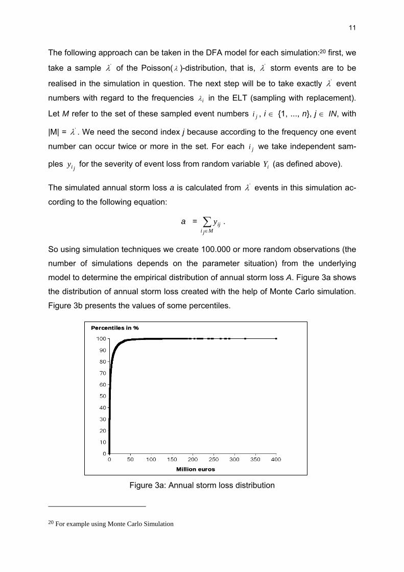
The following approach can be taken in the DFA model for each simulation:20 first, we

take a sample 'λ of the Poisson( λ )-distribution, that is, 'λ storm events are to be

realised in the simulation in question. The next step will be to take exactly 'λ event

numbers with regard to the frequencies iλ in the ELT (sampling with replacement).

Let M refer to the set of these sampled event numbers ji , i ∈ {1, ..., n}, j ∈ IN, with

|M| = 'λ . We need the second index j because according to the frequency one event

number can occur twice or more in the set. For each ji we take independent sam-

ples jiy for the severity of event loss from random variable iY (as defined above).

The simulated annual storm loss a is calculated from 'λ events in this simulation ac-

cording to the following equation:

a = ∑∈Mji

ijy .

So using simulation techniques we create 100.000 or more random observations (the

number of simulations depends on the parameter situation) from the underlying

model to determine the empirical distribution of annual storm loss A. Figure 3a shows

the distribution of annual storm loss created with the help of Monte Carlo simulation.

Figure 3b presents the values of some percentiles.

Figure 3a: Annual storm loss distribution

20 For example using Monte Carlo Simulation

Million euros

Percentiles in %

Million euros

Percentiles in %

12

Figure 3b: Percentiles of the annual storm loss distribution (see Figure 3a)

Here we want to make a short remark: Variability in event severity should still be

modelled as can be seen from Figure 3c. No variance was assumed in the individual

event severity on the ELT, eliminating the Beta-distribution described in the above

model. So in (**) we replace the random variable iZ by im . A comparison of the ta-

bles in Figure 3b and 3c shows that no large deviations can be deduced in the lower

and medium percentiles, whereas remarkable deviations can be recognised in the

very high percentiles (see maxima etc.), which may have a substantial impact on de-

termining risk capital requirement.

Figure 3c: Percentiles of the annual storm loss distribution without variance in single

events

Annual losses (without variance in single events)Percentiles in million eurosmean 5standard deviation 10median 1minimum 0maximum 28750% percentile 160% percentile 270% percentile 380% percentile 690% percentile 1499% percentile 4499,5% percentile 6099,9% percentile 11399,99% percentile 203

Annual lossesPercentiles in million eurosmean 5standard deviation 11median 1minimum 0maximum 40050% percentile 160% percentile 270% percentile 380% percentile 690% percentile 1399% percentile 4999,5% percentile 6799,9% percentile 11699,99% percentile 267

13

If several lines of business (divisions) are to be modelled, ELT can be generated for

the individual lines of business if there is enough data. There are two options for

modelling several lines of business using ELT. In the first option, the entries of the

division ELT can be aggregated per event number in the first step while the standard

deviation can be calculated assuming suitable correlation. The second step is to

simulate the total event, which can then be divided amongst the lines of business

affected according to the share of the division in the total expected value of the event

severity in the third step. In the second option, each line of business is modelled

separately and finally aggregated by event number. Here, suitable dependencies

(which have often a non-linear structure) between the random variables of event se-

verity need to be selected. We have used both of these methods in modelling build-

ing storm insurance and industrial storm insurance. These two methods yielded al-

most identical results.

3.2 Mathematical statistical approaches

In the mathematical statistical model the event frequency is assumed to be inde-

pendent from the event claim sizes which are assumed to be independent and identi-

cally distributed. So the assumptions of the collective model are assumed to be ful-

filled. The event severity and frequency distributions are fitted with the help of the

company’s own historical data (observations), adding PML from events with long re-

turn periods with losses that the company has not yet experienced. This modelling

approach uses only return periods and the associated PML for the insurance com-

pany itself, rather than complete ELT, as output from natural risks models.

The empirical claims data of the company should originate from a time period reach-

ing back as long as possible; the event loss should be extrapolated with suitable in-

dexes – such as the building cost index – to future years. Changes in portfolio – such

as the introduction of deductibles – should also be adequately taken into account.

Average claim sizes and degrees of exposure should be taken into consideration in

order to ensure that the scale of portfolio remains independent from the number of

14

the insured policies.21 Historical claims experience will usually be insufficient for the

choice of an appropriate model since very long return periods (such as 100, 200,

250, 500, 1,000, 10,000-year events, etc.) also need to be included. These seldom

events determine the tail part of the loss distribution, thus playing a major role in de-

termining the risk capital requirement of the company. Only using historical data in

order to fit the underlying distribution would generally only provide an insufficient ac-

count of possible losses in the future. This could lead to an underestimation in the

risk capital requirement of the company.

Empirical claims data is thus enriched with the PML from long return periods from the

natural risks models in order to fit the underlying severity distribution. The external

data serves to adapt the tail part of the catastrophe loss distribution that cannot be

fitted to a satisfactory extent by historical data, by adding claims with long return pe-

riods. This means that several distributions are fitted according to the maximum-

likelihood method (for estimating the parameters).22 Statistical goodness-of-fit tests

can then be used to select the best-fitting model from these models.23

Statistical tests can also show whether the external dates are appropriate in relation-

ship to historical in-house data. So it can be evaluated if the PML are adequate or too

high or too low for the portfolio. This addresses the problems arising from the wide

discrepancy between many results from various external studies for the same risk

and portfolio. The validation of the model is a very important but difficult process be-

cause it requires the comparison of losses from particular storm events with the

losses that the model would estimate for occurrences with the same physical charac-

teristics, given the same geographical distributions of exposed properties. These

data are often unavailable or not available in the quantity necessary for statistical

testing.24 The loss distributions calculated as a base for current portfolio structure

21 Natural risks models may also be referred to in fitting empirical (historical) in-house data to the current port-folio. These represent storms from the past and evaluate them taking the current portfolio into account.

22 This causes a parameter risk which has additionally to be modelled. An example for modelling the parameter risk in internal models is given in Diers, D. (2007b).

23 Examples of mainly quantitative test methods include the 2χ -test, Kolmogorov-Smirnov test and Anderson-Darling test. Apart from the quantitative test methods, more qualitative or intuitive methods such as the mean-excess plot, Hill plot, P-P plot and Q-Q plot may be used.

24 See Clark, K. (2002). Clark states further that “The nature of statistics is such that one can never prove that the sample is a true representation of the population. Statistical tests of significance merely provide confidence in-

15

should then be subject to continuous review and immediately adjusted for changing

conditions.

The approach to catastrophe modelling based on empirical data is often criticised

due to the lack of basis in historical loss development in estimating seldom return

periods. However, this objection also applies to geophysical models, as the parame-

ters they use are also derived from historical data. As Pohlhausen commented, ex-

trapolating the future from the past is not unproblematic. However, it is a sensible

activity. There is no other possibility for addressing future uncertainty.25

In the following the catastrophe-modelling approach using mathematical statistical

models will be presented, again taking storm events as an example. The modelling

proposal presented here requires the following definitions:

- NumR: number of risks insured,

- DE: random variable for the degree of exposure per event (number of risks af-

fected by the event as a percentage of the number of risks insured),

- MAX_DE: maximum degree of exposure = 100%,26

- AC: random variable for the average claim severity from one event, that is, the

claim severity from one event divided by the number of risks affected by this

event,

- λ: expected value for the number of events in the year to be modelled,

- MAX_Storm: maximum loss that can be caused by a storm event.

The random variable of claim severity CS is calculated as follows:

CS = Accept (NumR ⋅ DE ⋅ AC; NumR ⋅ DE ⋅ AC ≤ MAX_Storm),

with distribution function F for random variable DE:

DEF (x) = )_(

1DEMAXFX

XF (x), for x < MAX_DE, DEF (x) = 1 otherwise.

tervals for parameter estimates which are based on certain assumptions. These tests are used to choose be-tween alternatives or competing hypotheses.”

25 See Pohlhausen, R. (1999). 26 The maximum degree of loss can be less than 100% depending on the portfolio.

16

The Accept-function causes each case where the claim severity simulated exceeds

MAX_Storm to be simulated again until all of the results fall below MAX_Storm.27 We

can fit the underlying distributions for random variables X, which represents the de-

gree of exposure per event before maximum,28 and AC by suitable matching between

the in-house and external data, which represent the observations, according to the

statistical approach described above.

The next step is to model annual loss due to storm events. Following the collective

model the random variable of annual storm loss A can be represented as the sum of

the independent and identically distributed claim severities CSi that follow the same

distribution as CS and are assumed to be independent of random variable of event

frequency N:29

A = ∑=

N

iiCS

1.

We assume that N follows a Poisson-distribution with parameter λ, which can be es-

timated from historical data. Using Monte Carlo simulations a large number of ran-

dom observations (e.g. 100.000) can be simulated from the model in order to create

the empirical distribution of the annual storm loss.

This modelling approach together with the use of random variables of degree of ex-

posure and average claim severity presents the advantage that the underlying portfo-

lio size and structure are directly accounted for in the model. Here, it is absolutely

necessary to review how this model fits historically recorded annual loss due to

storms as well as external PML provided for annual loss. Additionally one can directly

fit the underlying event severity distribution CS using the statistical methods de-

scribed above and compare the results for validation.

27 Using the Accept-function represents the possibility of capping; however, this only applies in cases where only a few simulations are lying above the condition. If this is not the case, the selected model should be re-viewed for validity. An alternative approach in capping is the minimum function CS = MINIMUM(NumR ⋅ DE ⋅ AC; MAX_Storm). The two approaches lead to different results, however.

28 Before maximum means that the degree of exposure per event is limited by MAX_DE, which is omitted until this point.

29 According to the assumptions of the collective model degrees of exposure and average claim sizes are as-sumed to be independent and identically distributed as DE and AC respectively. If these assumptions hold in practice has to be verified. We use this modelling approach in order to be able to use this model for strategic decisions.

17

The final decision as to whether the distribution assumptions are adequate choices of

loss distributions, along with a final judgement as to whether the Poisson or the

Negative Binomial distribution – as example – is the adequate choice of the distribu-

tion of claim frequencies, should not be made until this point.30

Figure 4b shows the annual storm loss distribution and compares the results with the

empirical distribution (original data: empirical and external) for the storm insurance

divisions modelled here (Figures 4a). In order to improve the readability of the pres-

entation in Figure 4b we show the part of the distribution up to € 120 million. The

maximum is € 400 million.

Figure 4a: Empirical in-house data for annual storm claims and external data for long return periods (rp)

30 Refer to Rosemeyer / Klawa (2006), who studied the number of storms in Germany from 1970 to 1997 and identified the Negative Binomial distribution as the more valid distribution.

Million euros

Empirical in-house data

120

9284

6963

5647

4134

2621191614139875432

0

20

40

60

80

100

120

External data

100rp

150rp

200rp

250rp

400rp

500rp

1.000rp

Million euros

Empirical in-house data

120

9284

6963

5647

4134

2621191614139875432

0

20

40

60

80

100

120

External data

100rp

150rp

200rp

250rp

400rp

500rp

1.000rp

18

Figure 4b: Annual storm loss distribution vs. empirical distribution (in-house and ex-ternal data from Figure 4a)

Figure 5a shows the distribution of annual storm loss according to the mathematical

statistical model (black) and according to natural-risk models using ELT (red) from

Section 3.1 for comparison. Both graphs have a very similar curve, which means that

the ELT used fit well to observations for the lower percentile ranges. The agreement

in the upper percentile range (99% percentile and above) results from our use of long

return periods derived from the ELT (as observations) in the mathematical statistical

distribution fit. It also shows that the long return periods match our historical experi-

ence. In practice as described above, various sources are available to insurance

companies for long return periods whose results often widely fluctuate. Comparison

with in-house data usually helps solve this fluctuation. Figure 5b presents the values

of some percentiles.

No storm event loss

Empirical data fromthe company

(see Figure 4a)

External data (see Figure 4a)

Percentiles in %

Million euros

(Empirical) in-houseand external data

Annual stormloss distribution

No storm event loss

Empirical data fromthe company

(see Figure 4a)

External data (see Figure 4a)

Percentiles in %

Million euros

(Empirical) in-houseand external data

Annual stormloss distribution

19

Figure 5a: Annual storm loss distribution according to the mathematical statistical model (black) vs. modelling based on natural-risk models (red)

Figure 5b: Percentiles of annual storm loss distribution according to the mathematical statistical model (black) vs. modelling based on natural-risk models (red)

Modelling certain reinsurance contracts such as frequency cover requires a probabil-

ity distribution for the number of claims arising from storm events.

The random variable number of claims per event – NEi – can be calculated as fol-lows:

Million euros

Percentile in %

ELT

Statistical

Million euros

Percentile in %

ELT

Statistical

Million euros ELT Statisticalmean 5 5standard deviation 11 11median 1 2minimum 0 0maximum 400 40050% percentile 1 260% percentile 2 370% percentile 3 580% percentile 6 890% percentile 13 1498% percentile 36 3499% percentile 49 4799,5% percentile 67 6399,8% percentile 94 9299,9% percentile 116 120

20

NEi = NumR ⋅ DEi.

The modelling approach presented here is not based on different models for the dif-

ferent lines of business, as is usual in non-catastrophe claims modelling.31 So the

event losses have to be distributed amongst the lines of business affected. Distribu-

tion may be applied taking fixed keys, which can be derived from the company’s re-

cords. Individual portfolio structure should be taken into account. If, for example, the

company’s records or the use of natural risks models reveals that major storms have

a greater impact on a specific division (such as industrial storm insurance due to the

higher PML) than on other divisions (such as building or household) in comparison to

minor events, this effect should be given consideration.32 In these cases, the per-

centage key should not be fixed but should be applied dynamically, depending on the

claim severity of the event. Modelling catastrophe claims results in functional de-

pendencies between the divisions affected.33

Another aspect that needs to be considered when modelling event loss is the exten-

sion of simulation data with information on the time that the event takes place. This

information is necessary for adequately calculating cash-flows. An event that occurs

early in the year will mostly be settled in the same year, leading to a different cash-

flow situation that would arise for events occurring at the end of the year where the

most part of the settlement will be paid in the following year. Therefore, it is wise to

simulate an indicator as to whether the event occurs for example in the first or sec-

ond six months of the year.

So the probability p of a storm event taking place in the first six months is to be calcu-

lated on the basis of in-house data to be enriched with external information. This

yields the following weighting vector:

Weight (first six months; second six months) = (p; 1-p)

31 See for example Diers, D. (2007a) for attritional and large claims modelling in internal models. 32 This assumption must be justified (for example by internal records). 33 Additionally, the dependencies between the individual catastrophe risks (storms, earthquakes, hailstorms,

floods, etc.) must be represented. Modelling dependencies (which have often non-linear structures) in internal company models plays an important role in claim modelling. See for example Diers, D. (2007a). For the cop-ula approach see Pfeifer / Neslehova (2004).

21

This will facilitate simulating the occurrence of an event in the first or second six

months for each event.

3.3 Comparison of the two modelling approaches

Since catastrophe claims have a major impact on corporate strategy due to the high

level of risk involved, they must be adequately modelled in DFA models. On the one

hand modelling based on ELT from natural risks models can be validated using sta-

tistical modelling to review PML for long return periods. On the other hand the validity

of ELT for the shorter return periods can be checked with reference to empirical in-

house data.

The following presents the “advantages” and “disadvantages” of methods described

in Sections 3.1 and 3.2.

Modelling based on mathematical statistical methods encompass all of the his-

torical events, which are used to fit the underlying distributions. This aids plausibil-

ity testing on high PML, as these have to fit the historical losses (see Figure 4b).

Therefore, mathematical statistical models can and should be used to test the

plausibility of ELT as well.

Statistical models present another advantage in that the model is based on mod-

elling the random variables degree of loss and average claim severity, so that the

underlying portfolio size and structure are directly accounted for in the model. An-

other advantage is that model extensions can easily be made. This means the ef-

fects of strategies such as introduction of deductibles on the risk capital require-

ment can be modelled and quantified. This is not directly possible using ELT as a

basis, as ELT only reflect the effects of individual catastrophe events on the cur-

rent portfolio, meaning that the corporate strategies (affecting gross business be-

fore reinsurance) cannot be directly represented.

However, modelling based on ELT presents the distinct advantage of including all

events from the natural risks model into the model. Although either approach will

lead to a very similar curve in the annual loss distribution in our example (see Fig-

ures 5a and 5b), the number of events and loss severity may vary. This is unim-

portant at gross level for corporate strategy and risk capital calculation, as only

22

the annual loss is important here. However, there may be major differences in

annual loss distributions after reinsurance if excess-of-loss agreements by event

(event XLs) are considered, whose impact depends on the nature of the individual

event.

So both models should be applied as necessary depending on the actual issue

concerned in corporate strategy. Anyway they should be used for validation of the

other model.

4 Impact of the two modelling approaches on risk capital requirement

The loss resulting from catastrophe events can take on a very large scale, and there-

fore tie a significant share of the entire risk capital of a company.

The following will explain the effect of the different modelling approaches as de-

scribed here on risk capital requirement. We have taken value-at-risk VaR and tail-

value-at-risk TVaR as risk measure at a confidence level of 1-α = 0.998. Both risk

measures are often used in practice. The tail-value-at-risk for a real random variable

L is defined as follows:

TVaRα (L ) = E[L | L ≥ VaRα(L)].

TVaR is defined as the expected loss of α⋅100% worst cases, α ∈ (0.1).34 The value-

at-risk is defined as

VaRα (L ):= [ ]α−≥∈ 1)(:inf xFIRx L ,

where FL denotes the distribution function of the loss L.

In the following let A denote the random variable of the annual storm loss. We define

risk capital using the TVaR and VaR as risk measures with confidence level 99,8%

and the following random variable L (loss):

L = A – E(A),

34 There exist many publications where the tail-value-at-risk, which is recommended by IAA (2004), is criti-cised, see for example Pfeifer, D. (2004b), Rootzén / Klüppelberg (1999), McNeil / Embrechts / Frey (2005). A further discussion about the use of risk measures is absolutely necessary but exceeds the purpose of this pa-per.

23

where E(A) denotes the expected value.

Figure 6 shows that the risk capital requirements based on TVaR lie much beyond

those based on VaR because of the extremely high losses with very small probabili-

ties. The risk capital calculated using the confidence level of 99,8% is €135 respec-

tively €139 million for each of the modelling alternatives shown in Sections 3.1 and

3.2 (using TVaR). Note that the similar risk capital requirements result from the PML

for extreme events, which were used to fit the underlying distributions in the mathe-

matical statistical model and were taken from the ELT, as were applied to the ELT-

based model.

Strategic management often involves discussing alternatives for risk reduction in di-

visions with very high risk capital requirement, such as where the capital available is

exceeded. In those cases adequate reinsurance protection is an important factor.

Other concepts are possible in storm risk, such as the introduction of deductibles.

Since large numbers of claims with low average losses are typical of storm events,

even low deductibles will have a great effect. Figure 6 shows the risk capital require-

ment with a universal introduction of deductibles in our sample portfolio. Somewhat

lower deductibles for €250 and €500 have been assumed, as higher may otherwise

lead to the undesirable effect of losing customers due to the general unpopularity of

deductibles.

Modelling based on mathematical statistical methods as shown in Section 3.2 has

been adjusted to these altered conditions by exactly calculating the deductibles to

historical loss data according to as-if calculations. The relief from loss in the longer

return periods has also been approximated from as-if calculations. Modelling using

ELT requires the individual events to be fitted to conditions. Here, we have omitted

this step since this is only possible with direct access to natural risks models.

At €250 deductibles, the risk capital requirement decreases by around 24%, and a

clear reduction of 45% results from €500 deductibles. This confirms the positive ef-

fect of deductibles on the risk situation of the company with regard to storm loss.

However, successfully introducing deductibles heavily depends on customer accep-

24

tance (taking into account cross-selling and cross-cancellation effects). The market-

ing aspects should never be ignored in such strategic decisions.35

Figure 6: Value-at-risk and Tail-value-at-risk at a confidence level of 99.8% for an-

nual storm loss

5 Conclusion and outlook

Catastrophe modelling is especially important in internal modelling because catastro-

phe claims can tie a significant share of the entire risk capital of a company.

The previous sections have shown that natural risk models are a vital ingredient for

reliable statistical modelling. Modelling with mathematical statistical methods can be

used to review the suitability of PML in long return periods with reference to historical

data. Anyway both models (from Section 3.1 and 3.2) should be used for validation of

the other model.

With these models a variety of gross strategies such as introduction of deductibles

can be directly modelled. The effects of reinsurance contracts and alternative rein-

35 For the simuation study of this paper we used the simulation software of EMB Deutschland.

VaR 99,8%TVaR 99,8%

89 86

65

47

77

106

139135

0

20

40

60

80

100

120

140

ELT Math.-Stat. SB 250 SB 500

Million euros

Statistical Deductibles€250 €500

VaR 99,8%TVaR 99,8%

89 86

65

47

77

106

139135

0

20

40

60

80

100

120

140

ELT Math.-Stat. SB 250 SB 500

Million euros

Statistical Deductibles€250 €500

25

surance strategies such as event XL can be tested. The approach based on natural

risk models usually leads to results that reflect the risk situation of the company more

adequately since all of the events in the ELT are explicitly included in the model. As a

result, in future insurance companies should use own natural risks models, which

allow them to change the respective parameters for calculating the effects on man-

agement strategies (e.g. introduction of deductibles).

So in the areas of underwriting policy, changing insurance terms (as introduction of

deductibles, limits, etc.), expansion, withdrawal from special segments, reinsurance

buying, pricing, marketing, etc., these models can be an essential help for the man-

agement decisions in future.

Individual company modelling in DFA models create distributions of results of all dif-

ferent lines of business, reinsurance contracts, assets-classes, etc., as a basis for

defining important strategic indicators such as return on risk adjusted capital, eco-

nomic value added, economical profit and loss accounts, balance sheets, etc., by

using simulation methods.

The models described here represent an important step in supporting management

in a thorough value and risk-based corporate strategy that will lead to a lasting in-

crease in corporate value while providing solid support for risk management.

References

Allianz Group and World Wildlife Fund (2006): Climate Change and Insurance: An Agenda for Action in the United States, October 2006, [Download: http://www.allianz.com/Az_Cnt/az/_any/cma/contents/1260000/saObj_1260038_allianz_Climate_US_2006_e.pdf]

Clark, K. M. (2002): A Formal Approach to Catastrophe Risk Assessment and Man-agement, Proceedings of the Casualty Actuarial Society 1986, S. 69-92

D'Agostino, R.B.; Stephens, M. A. (1986): Goodness of Fit Techniques, New York: Marcel Dekker, Inc

Diers, D. (2007a): Interne Unternehmensmodelle in der Schaden- und Unfallversi-cherung – Entwicklung eines stochastischen internen Modells für die wert- und risi-koorientierte Unternehmenssteuerung und für die Anwendung im Rahmen von Sol-vency II, ifa-Verlag (www.ifa-ulm.de)

Diers, D. (2007b): Das Parameterrisiko – Ein Vorschlag zur Modellierung, Universität Ulm

26

Diers, D. (2008a): Der Einsatz mehrjähriger Interner Modelle zur Unterstützung von Managemententscheidungen. Supplement: Zeitschrift für die gesamte Versiche-rungswissenschaft, Volume 97, Issue 1

Diers, D.(2008b): Aspekte der rendite- und risikoorientierten Steuerung in der Scha-den- und Unfallversicherung. Schriftenreihe SCOR Deutschland, Nr. 7, Verlag Versi-cherungswirtschaft, Karlsruhe

Diers, D.(2009a): Strategic management of assets and liabilities using multi-year in-ternal risk models, Paper accepted for presentation at the 2009 annual meeting of American Risk and Insurance Association (ARIA)

Diers, D.(2009b): The use of multi-year internal models for management decisions in multi-year risk management, Paper accepted for presentation at ASTIN conference in Helsinki 2009

Dong, W. (2001): Building a More Profitable Portfolio, Modern Portfolio Theory with Application to Catastrophe Insurance, Reactions Publishing Group, London

Embrechts, P.; Lindskog, A. J., McNeil, A. J. (2001): Modelling Dependence with Copulas and Applications to Risk Management; working paper, ETH Zürich, Depart-ment of Mathematics, [http://www.gloriamundi.org/picsresources/peflam.pdf]

Embrechts, P.; McNeil, A. J.; Straumann, D. (2002): Correlation and Dependance in Risk Management: Properties and Pitfalls; Dempster, M. A. H. (Hrsg.): Risk Man-agement: Value at Risk and Beyond, Cambridge u. a., Cambridge University Press, 176-223

Frees, E. W.; Valdez, E. A. (1998): Understanding Relationships Using Copulas, in: North American Actuarial Journal (NAAJ), Vol. 2, No. 1, 1998, 1-25

Friedman, D. G. (1972): Insurance and the Natural Hazards, in: ASTIN Bulletin, 7. Jg. (1972), H., 4-58

GDV (2007): Kumul- und Großrisiken in Solvency II – Zur Modellierung und Kalibrie-rung der deutschen Anleitung der QIS3; [Download: http://visportal.gdv.org/archiv/Oeffentlich/Querschnitt/BW_Institut/1155_2007_anlage_anhang.pdf]

Hipp, Ch.; Michel, R. (1990): Risikotheorie: Stochastische Modelle und Statistische Methoden, Schriftenreihe Angewandte Versicherungsmathematik, Verlag VVW, Karlsruhe

International Actuarial Association IAA (2004): A Global Framework for Insurer Sol-vency Assessment; Research Report of the Insurer Solvency Assessment Working Party, Ottawa

Mack, T. (2002): Schadenversicherungsmathematik; Schriftenreihe Angewandte Versicherungsmathematik, DGVM, VVW Karlsruhe, Heft 28, 2.Auflage

McNeil, A. J.; Embrechts, P.; Frey, R. (2005): Quantitative Risk Management: Con-cepts Techniques Tools; Princeton Series in Finance, Princeton University Press, Princeton and Oxford

27

McNeil, A. J.; Saladin, T. (1997): The Peaks over Thresholds Method for Estimating High Quantiles of Loss Distributions, Proceedings of 28th International ASTIN Collo-quium [Download: http://www.math.ethz.ch/~mcneil/ftp/cairns.pdf]

Pfeifer, D. (2000): Wissenschaftliches Consulting im Rückversicherungsgeschäft: Modelle, Erfahrungen, Entwicklungen; Zeitschrift für Versicherungswesen 21 (2000), 771-777

Pfeifer, D. (2004): Solvency II: neue Herausforderungen an Schadenmodellierung und Risikomanagement? In: Albrecht, P., Lorenz, E. and Rudolph, B. (Eds.): Risiko-forschung und Versicherung – Festschrift für Elmar Helten zum 65. Geburtstag, Ver-lag Versicherungswirtschaft, 467 - 489

Pfeifer, D. (2004): VaR oder Expected Shortfall: Welche Risikomaße sind für Solven-cy II geeignet? Preprint, Universität Oldenburg, 2004

Pfeifer, D.; Neslehova, J. (2004): Modeling dependence in finance and insurance: the copula approach. Blätter der DGVFM Band XXVI, Heft 2, 177 – 191

Pohlhausen, R. (1999): Gedanken zur Überschwemmungsversicherung in Deutsch-land; Zeitschrift für die gesamte Versicherungswissenschaft 2/3 (1999), 457 - 467

Rosemeyer, J.C.; Klawa, M. (2004): Modellierung von Sturmserien mit Hilfe der Ne-gativbinomialverteilung; in: Zeitschrift für Versicherungswesen, 57. Jg., 153-156

Rootzén, H.; Klüppelberg, C. (1999): A single number can’t hedge against economic catastrophes, Ambio 28, No. 6, Royal Swedish Academy of Sciences

Straßburger, D. (2006): Risk Management and Solvency – Mathematical Methods in Theory and Practice, Dissertation an der Carl von Ossietzky Universität Oldenburg, 2006

Swiss Re (2002): Global non-life insurance in a time of capacity shortage, Sigma No. 4/2002

Swiss Re (2006): Measuring underwriting profitability of the non-life insurance indus-try, Sigma No. 3/2006

Whitaker, D. (2002): Catastrophe Modelling, in: Golden, N. (Eds.): Rational Reinsur-ance Buying, RISK Books, London, 103 - 122.

Woo, Gordon (1999): The mathematics of natural catastrophes, Imperial College Press