stochastic optimization part i: convex analysis and...

Stochastic OptimizationPart I: Convex analysis and

online stochastic optimization

† Taiji Suzuki

†Tokyo Institute of TechnologyGraduate School of Information Science and EngineeringDepartment of Mathematical and Computing Sciences

MLSS2015@Kyoto

1 / 73

Outline

1 Introduction

2 Short course to convex analysisConvexity and related conceptsDualitySmoothness and strong convexity

3 First order methodProximal gradient descentNesterov’s acceleration and optimal convergence

4 Online stochastic optimizationStochastic gradient descentStochastic regularized dual averaging

2 / 73

Lecture plan

Part I: introduction to stochastic optimization

Convex analysisFirst order method“Online” stochastic optimization method: SGD, SRDA

Part II: faster stochastic gradient methods and “batch” methods

AdaGrad, acceleration of SGD“Batch” stochastic optimization method: SDCA, SVRG, SAG

Part III: stochastic ADMM and distributed optimization

Stochastic ADMM for structured sparsityDistributed optimization (very shortly)

3 / 73

Outline

1 Introduction




4 / 73

Machine learning as optimization

Machine learning is a methodology to deal with a lot of uncertain data.

Generalization error minimization minθ∈Θ

EZ [ℓθ(Z )]

Empirical approximation minθ∈Θ

1

n

n∑i=1

ℓθ(zi )

Stochastic optimization is an intersection of learning and optimization.5 / 73

New data inputMassive data

x1x2x3x4....

Recently stochastic optimization is used to treat huge data.

1

n

n∑i=1

ℓθ(zi )︸︷︷︸Huge

+ψ(θ)

How to optimize this in efficient way?Do we need to go through the whole data at every iteration? 6 / 73

History of stochastic optimization for ML

1951 Robbins and Monro Stochastic approximationfor root finding problem

1957 Rosenblatt Perceptron

1978 Nemirovskii and Yudin Robustification via averagingfor non-smooth obj.

1988 Ruppert Robust step size policy and averaging1992 Polyak and Juditsky for smooth obj.

1998 Bottou Online stochastic optimization2004 Bottou and LeCun for large scale ML task

2009-2012

Singer and Duchi; Duchi

et al.; Xiao

FOBOS, AdaGrad, RDA

2012- Le Roux et al. Linear convergence on batch data2013 Shalev-Shwartz and Zhang (SAG,SDCA,SVRG)

Johnson and Zhang7 / 73

Overview of stochastic optimization

minx

f (x)

Stochastic approximation (SA)Optimization for systems with uncertainty,e.g., machine control, traffic management, social science, and so on.gt = ∇f (x (t)) + ξt is observed where ξt is noise (typically i.i.d.).

Stochastic approximation for machine learning and statisticsTypically generalization error minimization:

minx

f (x) = minx

EZ [ℓ(Z , x)].

gt = ∇ℓ(zt , x (t)) is observed where zt ∼ P(Z ) is i.i.d. data.ℓ(z , x) is a loss function:e.g., logistic loss ℓ((w , y), x) = log(1 + exp(−yw⊤x)) forz = (w , y) ∈ Rp × {±1}.Used for huge dataset.We don’t need exact optimization. Optimization with certainprecision (typically O(1/n)) is sufficient.

8 / 73

Two types of stochastic optimization

Online type stochastic optimization:

We observe data sequentially.Each observation is used just once (basically).

minx

EZ [ℓ(Z , x)]

Batch type stochastic optimization

The whole sample has been already observed.We may use training data multiple times.

minx

1

n

n∑i=1

ℓ(zi , x)

9 / 73

Summary of convergence rates

Online methods (expected risk minimization):GR√T

(non-smooth, non-strongly convex)

G 2

µT(non-smooth, strongly convex)

σR√T

+R2L

T 2(smooth, non-strongly convex)

σ2

µT+ exp

(−√µ

LT

)(smooth, strongly convex)

Batch methods (empirical risk minimization)

exp(− 1

n+µLT)(smooth loss, strongly convex reg)

exp

(− 1

n+√

nµL

T

)(smooth loss, strongly convex reg with acceleration)

G : upper bound of norm of gradient, R: diameter of the domain,L: smoothness, µ: strong convexity, σ: variance of the gradient

10 / 73

Example of empirical risk minimization:High dimensional data analysis

Redundant information deteriorates the estimation accuracy.

Bio-informatics Text data Image data11 / 73

Sparse estimation

Cut off redundant information → sparsity

R. Tsibshirani (1996). Regression shrinkage and selection via the lasso. J. Royal.

Statist. Soc B., Vol. 58, No. 1, pages 267–288.

12 / 73

Lasso estimator

Lasso [L1 regularization]

βLasso = argminβ∈Rp

∥Y − Xβ∥2 + λ∥β∥1

where ∥β∥1 =∑p

j=1 |βj |.

Convex optimization

L1norm is the convex hull of L0normon [−1, 1]p (the largest convex functionwhich supports from below).

L1norm is the Lovasz extension of thecardinality function.

More generally for a loss function ℓ (logistic loss, hinge loss, ...)

minx

{n∑

i=1

ℓ(zi , x) + λ∥x∥1

}

13 / 73

Lasso estimator

Lasso [L1 regularization]

βLasso = argminβ∈Rp

∥Y − Xβ∥2 + λ∥β∥1

where ∥β∥1 =∑p

j=1 |βj |.

Convex optimization

L1norm is the convex hull of L0normon [−1, 1]p (the largest convex functionwhich supports from below).

L1norm is the Lovasz extension of thecardinality function.

More generally for a loss function ℓ (logistic loss, hinge loss, ...)

minx

{n∑

i=1

ℓ(zi , x) + λ∥x∥1

}13 / 73

Outline

1 Introduction




14 / 73

Regularized empirical risk minimization

Basically, we want to solve

Empirical risk minimization:

minx∈Rp

1

n

n∑i=1

ℓ(zi , x).

Regularized empirical risk minimization:

minx∈Rp

1

n

n∑i=1

ℓ(zi , x) + ψ(x).

In this lecture, we assume ℓ and ψ are convex.→ convex analysis to exploit the properties of convex functions.

15 / 73

Outline

1 Introduction




16 / 73

Convex set

Definition (Convex set)

A convex set is a set that contains the segment connecting two points inthe set:

x1, x2 ∈ C =⇒ θx1 + (1− θ2)x2 ∈ C (θ ∈ [0, 1]).

Convex set Non-convex set Non-convex set

17 / 73

Epigraph and domainLet R := R ∪ {∞}.

Definition (Epigraph and domain)

The epigraph of a function f : Rp → R is given by

epi(f ) := {(x , µ) ∈ Rp+1 : f (x) ≤ µ}.

The domain of a function f : Rp → R is given by

dom(f ) := {x ∈ Rp : f (x) <∞}.

epigraph

domain( ]

18 / 73

Convex function

Let R := R ∪ {∞}.

Definition (Convex function)

A function f : Rp → R is a convex function if f satisfies

θf (x) + (1− θ)f (y) ≥ f (θx + (1− θ)y) (∀x , y ∈ Rp, θ ∈ [0, 1]),

where ∞+∞ = ∞, ∞ ≤ ∞.

Convex Non-convex

f is convex ⇔ epi(f ) is a convex set.19 / 73

Proper and closed convex function

If the domain of a function f is not empty (dom(f ) = ∅), f is calledproper.

If the epigraph of a convex function f is a closed set, then f is calledclosed.(We are interested in only a proper closed function in this lecture.)

Even if f is closed, it’s domain is not necessarily closed (even for 1D).

“f is closed” does not imply“f is continuous.”

Closed convex function is continuous on a segment in its domain.

Closed function is “lower semicontinuity.”

20 / 73

Convex loss functions (regression)

All well used loss functions are (closed) convex. The followings are convexw.r.t. u with a fixed label y ∈ R.

Squared loss: ℓ(y , u) = 12(y − u)2.

τ -quantile loss: ℓ(y , u) = (1− τ)max{u − y , 0}+ τ max{y − u, 0}.for some τ ∈ (0, 1). Used for quantile regression.ϵ-sensitive loss: ℓ(y , u) = max{|y − u| − ϵ, 0} for some ϵ > 0. Usedfor support vector regression.

f-y-3 -2 -1 0 1 2 30

1

2

3 τ-quantile

-sensitive

Squared

Huber

21 / 73

Convex surrogate loss (classification)

y ∈ {±1}Logistic loss: ℓ(y , u) = log((1 + exp(−yu))/2).Hinge loss: ℓ(y , u) = max{1− yu, 0}.Exponential loss: ℓ(y , u) = exp(−yu).Smoothed hinge loss:

ℓ(y , u) =

0, (yu ≥ 1),12 − yu, (yu < 0),12(1− yu)2, (otherwise).

yf-3 -2 -1 0 1 2 30

1

2

3

40-1Logistic

expHinge

Smoothed-hinge

22 / 73

Convex regularization functions

Ridge regularization: R(x) = ∥x∥22 :=∑p

j=1 x2j .

L1 regularization: R(x) = ∥x∥1 :=∑p

j=1 |xj |.

Trace norm regularization: R(X ) = ∥X∥tr =∑min{q,r}

k=1 σj(X )where σj(X ) ≥ 0 is the j-th singular value.

-1 -0.8 -0.6 -0.4 -0.2 0 0.2 0.4 0.6 0.8 1-1

-0.8

-0.6

-0.4

-0.2

0

0.2

0.4

0.6

0.8

1

Bridge (=0.5)L1RidgeElasticnet

1n

∑ni=1(yi − z⊤i x)2 + λ∥x∥1: Lasso

1n

∑ni=1 log(1 + exp(−yiz

⊤i x)) + λ∥X∥tr: Low rank matrix recovery

23 / 73

Other definitions of sets

Convex hull: conv(C ) is the smallest convex set that contains a setC ⊆ Rp.

Affine set: A set A is an affine set if and only if ∀x , y ∈ A, the line thatintersects x and y lies in A: λx + (1− λ)y ∀λ ∈ R.

Affine hull: The smallest affine set that contains a set C ⊆ Rp.Relative interior: ri(C ). Let A be the affine hull of a convex set C ⊆ Rp.

ri(C ) is a set of internal points with respect to the relativetopology induced by the affine hull A.

Convex hullAffine hull

Relative interior

24 / 73

Continuity of a closed convex function

Theorem

For a (possibly non-convex) function f : Rp → R, the following threeconditions are equivalent to each other.

1 f is lower semi-continuous.

2 For any converging sequence {xn}∞n=1 ⊆ Rp s.t. x∞ = limn xn,lim infn f (xn) ≥ f (x∞).

3 f is closed.

Remark: Any convex function f is continuous in ri(dom(f )). The continuity

could be broken on the boundary of the domain.

25 / 73

Outline

1 Introduction




26 / 73

Subgradient

We want to deal with non-differentiable function such as L1 regularization.To do so, we need to define something like gradient.

Definition (Subdifferential, subgradient)

For a proper convex function f : Rp → R, the subdifferential of f atx ∈ dom(f ) is defined by

∂f (x) := {g ∈ Rp | ⟨x ′ − x , g⟩+ f (x) ≤ f (x ′) (∀x ′ ∈ Rp)}.

An element of the subdifferential is called subgradient.

f(x)

x

Subgradient

Figure: Subgraient

27 / 73

Properties of subgradient

Subgradient does not necessarily exist (∂f (x) could be empty).f (x) = x log(x) (x ≥ 0) is proper convex but not subdifferentiable at x = 0.

Subgradient always exists on ri(dom(f )).

If f is differentiable at x , its gradient is the unique element of subdiff.

∂f (x) = {∇f (x)}.

If ri(dom(f )) ∩ ri(dom(h)) = ∅, then∂(f + h)(x) = ∂f (x) + ∂h(x)

= {g + g ′ | g ∈ ∂f (x), g ′ ∈ ∂h(x)}(∀x ∈ dom(f ) ∩ dom(h)).

For all g ∈ ∂f (x) and all g ′ ∈ ∂f (x ′) (x , x ′ ∈ dom(f )),

⟨g − g ′, x − x ′⟩ ≥ 0.

28 / 73

Properties of subgradient

Subgradient does not necessarily exist (∂f (x) could be empty).f (x) = x log(x) (x ≥ 0) is proper convex but not subdifferentiable at x = 0.

Subgradient always exists on ri(dom(f )).If f is differentiable at x , its gradient is the unique element of subdiff.

∂f (x) = {∇f (x)}.

If ri(dom(f )) ∩ ri(dom(h)) = ∅, then∂(f + h)(x) = ∂f (x) + ∂h(x)

= {g + g ′ | g ∈ ∂f (x), g ′ ∈ ∂h(x)}(∀x ∈ dom(f ) ∩ dom(h)).

For all g ∈ ∂f (x) and all g ′ ∈ ∂f (x ′) (x , x ′ ∈ dom(f )),

⟨g − g ′, x − x ′⟩ ≥ 0.

28 / 73

Legendre transform

Defines the other representation on the dual space (the space of gradients).

Definition (Legendre transform)

Let f be a (possibly non-convex) function f : Rp → R s.t. dom(f ) = ∅.Its convex conjugate is given by

f ∗(y) := supx∈Rp

{⟨x , y⟩ − f (x)}.

The map from f to f ∗ is called Legendre transform.

f(x)

f*(y)

line with gradient y

xx*

0

f(x*)

29 / 73

Examples

f (x) f ∗(y)

Squared loss 12x2 1

2y 2

Hinge loss max{1− x , 0}

{y (−1 ≤ y ≤ 0),

∞ (otherwise).

Logistic loss log(1 + exp(−x)){(−y) log(−y) + (1 + y) log(1 + y) (−1 ≤ y ≤ 0),

∞ (otherwise).

L1 regularization ∥x∥1

{0 (maxj |yj | ≤ 1),

∞ (otherwise).

Lp regularization∑d

j=1 |xj |p ∑d

j=1p−1

pp

p−1|yj |

pp−1

(p > 1)

0

0 1

logistic dual of logistic

L1-norm dual

30 / 73

Properties of Legendre transformf ∗ is a convex function even if f is not.f ∗∗ is the closure of the convex hull of f :

f ∗∗ = cl(conv(f )).

Corollary

Legendre transform is a bijection from the set of proper closed convexfunctions onto that defined on the dual space.

f (proper closed convex) ⇔ f ∗ (proper closed convex)

0 1 2 3 4

-6

-4

-2

0

2

4

6f(x)cl.conv.

31 / 73

Connection to subgradient

Lemma

y ∈ ∂f (x) ⇔ f (x) + f ∗(y) = ⟨x , y⟩ ⇔ x ∈ ∂f ∗(y).

∵ y ∈ ∂f (x) ⇒ x = argmaxx ′∈Rp

{⟨x ′, y⟩ − f (x ′)}

(take the “derivative” of ⟨x ′, y⟩ − f (x ′))

⇒ f ∗(y) = ⟨x , y⟩ − f (x).

Remark: By definition, we always have

f (x) + f ∗(y) ≥ ⟨x , y⟩.

→ Young-Fenchel’s inequality.

32 / 73

⋆ Fenchel’s duality theorem

Theorem (Fenchel’s duality theorem)

Let f : Rp → R, g : Rq → R be proper closed convex, and A ∈ Rq×p.Suppose that either of condition (a) or (b) is satisfied, then it holds that

infx∈Rp

{f (x) + g(Ax)} = supy∈Rq

{−f ∗(A⊤y)− g∗(−y)}.

� �(a) ∃x ∈ Rp s.t. x ∈ ri(dom(f )) and Ax ∈ ri(dom(g)).

(b) ∃y ∈ Rq s.t. A⊤y ∈ ri(dom(f ∗)) and −y ∈ ri(dom(g∗)).� �If (a) is satisfied, there exists y∗ ∈ Rq that attains sup of the RHS.If (b) is satisfied, there exists x∗ ∈ Rp that attains inf of the LHS.Under (a) and (b), x∗, y∗ are the optimal solutions of the each side iff

A⊤y∗ ∈ ∂f (x∗), Ax∗ ∈ ∂g∗(−y∗).

→ Karush-Kuhn-Tucker condition.33 / 73

Equivalence to the separation theorem

Convex

Concave

34 / 73

Applying Fenchel’s duality theorem to RERM

RERM (Regularized Empirical Risk Minimizatino):Let ℓi (z

⊤i x) = ℓ(yi , z

⊤i x) where (zi , yi ) is the input-output pair of the i-th

observation.� �(Primal) inf

x∈Rp

{n∑

i=1

ℓi (z⊤i x)︸︷︷︸ + ψ(x)

}

f (Zx)� �[Fenchel’s duality theorem]

infx∈Rp

{f (Zx) + ψ(x)} = − infy∈Rn

{f ∗(y) + ψ∗(−Z⊤y)}

� �(Dual) sup

y∈Rn

{n∑

i=1

ℓ∗i (yi ) + ψ∗(−Z⊤y)

}� �This fact will be used to derive dual coordinate descent alg. 35 / 73

Outline

1 Introduction




36 / 73

Smoothness and strong convexity

Definition

Smoothness: the gradient is Lipschitz continuous:

∥∇f (x)−∇f (x ′)∥ ≤ L∥x − x ′∥.

Strong convexity: ∀θ ∈ (0, 1), ∀x , y ∈ dom(f ),

µ

2θ(1− θ)∥x − y∥2 + f (θx + (1− θ)y) ≤ θf (x) + (1− θ)f (y).

0 0 0

Smooth butnot strongly convex

Smooth andStrongly convex

Strongly convex butnot smooth

37 / 73

Duality between smoothness and strong convexity

Smoothness and strong convexity is in a relation of duality.

Theorem

Let f : Rp → R be proper closed convex.

f is L-smooth ⇐⇒ f ∗ is 1/L-strongly convex.

logistic loss its dual function

0

0 1

Smooth butnot strongly convex

Strongly convex butnot smooth

(gradient → ∞)

38 / 73

Outline

1 Introduction




39 / 73

Regularized learning problem

Lasso:

minx∈Rp

1

n

n∑i=1

(yi − z⊤i x)2 + ∥x∥1︸︷︷︸regularization

.

General regularized learning problem:

minx∈Rp

1

n

n∑i=1

ℓ(zi , x) + ψ(x).

Difficulty: Sparsity inducing regularization is usually non-smooth.

40 / 73

First order optimization

xt-1xtxt+1

Optimization methods that use only the function value f (x) and thefirst order gradient g ∈ ∂f (x).Computation per iteration is light, and suited for high dimensionalproblems.Newton method is a second order method.

41 / 73

Outline

1 Introduction




42 / 73

Gradient descent

Let f (x) =∑n

i=1 ℓ(zi , x).minx

f (x).

Subgradient method

Differentiable f (x):xt = xt−1 − ηt∇f (xt−1).

43 / 73

Gradient descent

Let f (x) =∑n


f (x).

Subgradient method

Subdifferentiable f (x):

gt ∈ ∂f (xt−1),

xt = xt−1 − ηtgt .

43 / 73

Gradient descent

Let f (x) =∑n


f (x).

Subgradient method (equivalent formula)

Subdifferentiable f (x):

xt = argminx

{⟨x , gt⟩+

1

2ηt∥x − xt−1∥2

},

where gt ∈ ∂f (xt−1).

Proximal point algorithm:

xt = argminx

{f (x) +

1

2ηt∥x − xt−1∥2

}.

f (xt) → optimum for any convex f and ηt = η > 0 (Guler, 1991).

If f (x) is strongly convex: f (xt)− f (x∗) ≤ 12η

(1

1+ση

)t−1

∥x0 − x∗∥2.43 / 73

Proximal gradient descent

Let f (x) =∑n

i=1 ℓ(zi , x).

minx

f (x) + ψ(x).


xt = argminx

{⟨x , gt⟩+ ψ(x) +

1

2ηt∥x − xt−1∥2

}= argmin

x

{ηtψ(x) +

1

2∥x − (xt−1 − ηtgt)∥2

}where gt ∈ ∂f (xt−1).

The update rule is given by proximal mapping:

prox(q|ψ) = argminx

{ψ(x) +

1

2∥x − q∥2

}→ By using the proximal mapping, we can avoid bad properties (e.g.,non-smoothness) of ψ. 44 / 73

Example

L1 regularization: ψ(x) = C∥x∥1.

xt,j = STCηt (xt−1,j − ηtgt,j) (j-th component)

whereSTC (q) = sign(q)max{|q| − C , 0}.

→ Unimportant elements are forced to be 0.

For many practically used regularizations, analytic form is obtained.

45 / 73

Example of proximal mapping (cont.)

Trace norm: ψ(X ) = C∥X∥tr = C∑

j σj(X ) (sum of singular values).Let

Xt−1 − ηtGt = U diag(σ1, . . . , σd)V ,

then

Xt = U

STCηt (σ1). . .

STCη(σd)

V .

46 / 73

Convergence of proximal gradient descent

Strong convexity and smoothness of f determines the convergence rate.

xt = prox(xt−1 − ηtgt |ηtψ(x)).

property of f µ-Strongly convex non-strongly conv

γ-Smooth exp

(−t

µ

γ

)γ

t

Non-smooth1

µt

1√t

The step size ηt should be appropriately chosen.Setting of ηt Strongly conv non-strongly conv

Smooth 1γ

1γ

Non-smooth 2µt

1√t

To achieve this convergence rate, we need to take an average of {xt}tappropriately; Polyak-Ruppert averaging, polynomially decaying averaging.

47 / 73

Convergence of proximal gradient descent

Strong convexity and smoothness of f determines the convergence rate.

xt = prox(xt−1 − ηtgt |ηtψ(x)).

property of f µ-Strongly convex non-strongly conv

γ-Smooth exp

(−t

√µ

γ

)γ

t2

Non-smooth1

µt

1√t

The step size ηt should be appropriately chosen.Setting of ηt Strongly conv non-strongly conv

Smooth 1γ

1γ

Non-smooth 2µt

1√t

To achieve this convergence rate, we need to take an average of {xt}tappropriately; Polyak-Ruppert averaging, polynomially decaying averaging.Convergence for smooth loss can be improved by Nesterov’sacceleration.→ Optimal rate

47 / 73

Outline

1 Introduction




48 / 73

Nesterov’s acceleration (non-strongly convex)minx{f (x) + ψ(x)}Assumption: f (x) is γ-smooth.

Nesterov’s acceleration scheme

Let s1 = 1 and η = 1γ , and iterate the following for t = 1, 2, . . .

1 Let gt ∈ ∂f (yt), and update xt = prox(yt − ηgt |ηψ).

2 Set st+1 =1+√

1+4s2t2 .

3 Update yt+1 = xt +(st−1st+1

)(xt − xt−1).

If f is γ-smooth, then

f (xt)− f (x∗) ≤ 2γ∥xt − x∗∥t2

.

This is also called Fast Iterative Shrinkage Thresholding Algorithm (FISTA)(Beck and Teboulle, 2009).

The step size η = 1/γ can be adaptively determined: back-trackingtechnique.

49 / 73

Nesterov’s acceleration (strongly convex)minx{f (x) + ψ(x)}Assumption: f (x) is γ-smooth and µ-strongly convex. (it must be γ > µ)

Nesterov’s acceleration scheme

Let A1 = 1, α1 = γ/µ and η = 1γ , and iterate the following for

t = 1, 2, . . .

1 Let gt ∈ ∂f (yt), and update xt = prox(yt − ηgt |ηψ).2 Set αt+1 > 1 so that (γ − µ)α2

t+1 − (2γ + At)αt+1 + γ = 0, and letAt+1 = At/αt+1.

3 Update yt+1 = xt +(

µ+At

(γ−µ)(αt+1−1)(αt−1)

)(xt − xt−1).

If f is γ-smooth and µ-strongly convex, then

f (xt)− f (x∗) ≤ γ

(1−

√γ

µ

)t

∥x0 − x∗∥2.

50 / 73

51 / 73

Iteration0 20 40 60 80 100 120

Rel

ativ

e ob

ject

ive

(f(x t)

- f* )

10-8

10-6

10-4

10-2

100

102

104

NormalNesterov

Nesterov’s acceleration v.s. normal gradient descentLasso: n = 8, 000, p = 500.

52 / 73

Outline

1 Introduction




53 / 73

Two types of stochastic optimization

Online type stochastic optimization:

We observe data sequentially.We don’t need to wait until the whole sample is obtained.Each observation is obtained just once (basically).

minx

EZ [ℓ(Z , x)]

Batch type stochastic optimization

The whole sample has been already observed.We can make use of the (finite and fixed) sample size.We may use sample multiple times.

minx

1

n

n∑i=1

ℓ(zi , x)

54 / 73

Online method

You don’t need to wait until the whole sample arrives.Update the parameter at each data observation.

zt-1 z

txt

xt+1

P(z)

Observe ObserveUpdate Update

storage New data input

minx

E[ℓ(Z , x)] + ψ(x) ≃ minx

1

T

T∑t=1

ℓ(zt , x) + ψ(x)

55 / 73

The objective of online stochastic optimization

Let ℓ(z , x) be a loss of x for an observation z .

(Expected loss) L(x) = EZ [ℓ(Z , x)]

or

(EL with regularization) Lψ(x) = EZ [ℓ(Z , x)] + ψ(x)

The distribution of Z could be

the true population→ L(x) is the generalization error.

an empirical distribution of stored data in a storage→ L (or Lψ) is the (regularized) empirical risk.

Online stochastic optimization itself is learning!

56 / 73

Outline

1 Introduction




57 / 73

Three steps to stochastic gradient descent

E[ℓ(Z , x)] =

∫ℓ(Z , x)dP(Z )

≃(1)ℓ(zt , xt−1) (sampling)

≃(2)

⟨∇xℓ(zt , xt−1), x⟩ (linearlization)

The approximation is correct just around xt−1.

minx

E[ℓ(Z , x)] ≃(3)

minx

{⟨∇xℓ(zt , xt−1), x⟩+

1

2ηt∥x − xt−1∥2

}(proximation)

xt-158 / 73

Stochastic gradient descent (SGD)

SGD (without regularization)

Observe zt ∼ P(Z ), and let ℓt(x) := ℓ(zt , x).

Calculate subgradient:

gt ∈ ∂xℓt(xt−1).

Update x asxt = xt−1 − ηtgt .

We just need to observe one training data zt at each iteration.→ O(1) computation per iteration (O(n) for batch gradient descent).

We do not need to go through the whole sample {zi}ni=1

Reminder: prox(q|ψ) := argminx{ψ(x) + 1

2∥x − q∥2}.

59 / 73

Stochastic gradient descent (SGD)

SGD (with regularization)


Calculate subgradient:

gt ∈ ∂xℓt(xt−1).

Update x asxt = prox(xt−1 − ηtgt |ηtψ).

We just need to observe one training data zt at each iteration.→ O(1) computation per iteration (O(n) for batch gradient descent).

We do not need to go through the whole sample {zi}ni=1

Reminder: prox(q|ψ) := argminx{ψ(x) + 1

2∥x − q∥2}.

59 / 73

Convergence analysis of SGD

Assumption

(A1) E[∥gt∥2] ≤ G 2.

(A2) E[∥xt − x∗∥2] ≤ D2.

Theorem

Let xT = 1T+1

∑Tt=0 xt . For ηt =

η0√t, it holds

Ez1:T [Lψ(xT )− Lψ(x∗)] ≤ η0G

2 + D2/η0√T

.

For η0 =DG , we have

2GD√T.

This is minimax optimal (up to constant).

G is independent of ψ thanks to the proximal mapping. Note that∥∂ψ(x)∥ ≤ C

√p for L1-reg.

60 / 73

Convergence analysis of SGD (strongly convex)

Assumption

(A1) E[∥gt∥2] ≤ G 2.

(A3) Lψ is µ-strongly convex.

Theorem

Let xT = 1T+1

∑Tt=0 xt . For ηt =

1µt , it holds

Ez1:T [Lψ(xT )− Lψ(x∗)] ≤ G 2 log(T )

Tµ.

Better than non-strongly convex situation.But, this is not minimax optimal.The bound is tight (Rakhlin et al., 2012).

61 / 73

Polynomial averaging for strongly convex risk

Assumption

(A1) E[∥gt∥2] ≤ G 2.

(A3) Lψ is µ-strongly convex.

Modify the update rule as

xt = prox

(xt−1 − ηt

t

t + 1gt |ηtψ

),

and take the weighted average xT =2

(T + 1)(T + 2)

T∑t=0

(t + 1)xt .

Theorem

For ηt =2µt , it holds Ez1:T [Lψ(xT )− Lψ(x

∗)] ≤ 2G 2

Tµ.

log(T ) is removed.This is minimax optimal (explained later).

62 / 73

Remark on polynomial averaging

xT =2

(T + 1)(T + 2)

T∑t=0

(t + 1)xt

O(T ) computation? No.xT can be efficiently updated:

xt =t

t + 2xt−1 +

2

t + 2xt .

63 / 73

General step size and weighting policy

Let st (t = 1, 2, . . . ,T +1) be a positive sequence such that∑T+1

t=1 st = 1.

xt = prox

(xt−1 − ηt

stst+1

gt |ηtψ)

(t = 1, . . . ,T )

xT =T∑t=0

st+1xt .

Assumption: (A1) E[∥gt∥2] ≤ G 2, (A2) E[∥xt − x∗∥2] ≤ D2, (A3) Lψ is

µ-strongly convex.

Theorem

Ez1:T [Lψ(xT )− Lψ(x∗)]

≤T∑t=1

st+1ηt+1

2G 2 +

T−1∑t=0

max{ st+2

ηt+1− st+1(

1ηt

+ µ), 0}D2

2

As for t = 0, we set 1/η0 = 0 .64 / 73

Special case

Let the weight proportion to the step size (step size could be seen asimportance):

st =ηt∑T+1τ=1 ητ

.

In this setting, the previous theorem gives

Ez1:T [Lψ(xT )− Lψ(x∗)] ≤

∑Tt=1 η

2tG

2 + D2

2∑T

t=1 ηt� �∞∑t=1

ηt = ∞

∞∑t=1

η2t <∞

ensures the convergence.� �65 / 73

Outline

1 Introduction




66 / 73

Stochastic regularized dual averaging (SRDA)

The second assumption E[∥xt − x∗∥2] ≤ D2 can be removed by using dualaveraging (Nesterov, 2009, Xiao, 2009).

SRDA


Calculate gradient: gt ∈ ∂xℓt(xt−1).

Take the average of the gradients:

gt =1

t

t∑τ=1

gτ .

Update as

xt = argminx∈Rp

{⟨gt , x⟩+ ψ(x) +

1

2ηt∥x∥2

}= prox(−ηt gt |ηtψ).

The information of old observations is maintained by taking average ofgradients.

67 / 73

Convergence analysis of SRDA

Assumption(A1) E[∥gt∥2] ≤ G 2.(A2) E[∥xt − x∗∥2] ≤ D2.

Theorem

Let xT = 1T+1

∑Tt=0 xt . For ηt = η0

√t, it holds

Ez1:T [Lψ(xT )− Lψ(x∗)] ≤ η0G

2 + ∥x∗ − x0∥2/η0√T

.

If ∥x∗ − x0∥ ≤ R, then for η0 =RG , we have

2RG√T.

This is minimax optimal (up to constant).The norm of intermediate solution xt is well controlled. Thus (A2) isnot required.

68 / 73

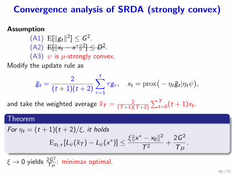
Convergence analysis of SRDA (strongly convex)

Assumption

(A1) E[∥gt∥2] ≤ G 2.

(A2) E[∥xt − x∗∥2] ≤ D2.

(A3) ψ is µ-strongly convex.

Modify the update rule as

gt =2

(t + 1)(t + 2)

t∑τ=1

τgτ , xt = prox(− ηt gt |ηtψ

),

and take the weighted average xT = 2(T+1)(T+2)

∑Tt=0(t + 1)xt .

Theorem

For ηt = (t + 1)(t + 2)/ξ, it holds

Ez1:T [Lψ(xT )− Lψ(x∗)] ≤ ξ∥x∗ − x0∥2

T 2+

2G 2

Tµ.

ξ → 0 yields 2G2

Tµ : minimax optimal.

69 / 73

General convergence analysis

Let the weight st > 0 (t = 1, . . . ) is any positive sequence. We generalizethe update rule as

gt =

∑tτ=1 sτgτ∑t+1τ=1 sτ

,

xt = prox(−ηt gt |ηtψ) (t = 1, . . . ,T ).

Let the weighted average of (xt)t be xT =∑T

τ=0 sτ+1xτ∑Tτ=0 sτ+1

.

Assumption: (A1) E[∥gt∥2] ≤ G 2, (A3) Lψ is µ-strongly convex (µ can be 0).

Theorem

Suppse that ηt/(∑t+1

τ=1 sτ ) is non-decreasing, then

Ez1:T [Lψ(xT )− Lψ(x∗)]

≤ 1∑T+1t=1 st

(T+1∑t=1

s2t2[(∑t

τ=1 sτ )(µ+ 1/ηt−1)]G 2 +

∑T+2t=1 st

2ηT+1∥x∗ − x0∥2

).

70 / 73

Computational cost and generalization error

The optimal learning rate for a strongly convex expected risk(generalization error) is O(1/n) (n is the sample size).

To achieve O(1/n) generalization error, we need to decrease thetraining error to O(1/n).

Normal gradient des. SGD

Time per iteration n 1Number of iterations until ϵ error log(1/ϵ) 1/ϵ

Time until ϵ error n log(1/ϵ) 1/ϵTime until 1/n error n log(n) n

(Bottou, 2010)

SGD is O(log(n)) faster with respect to the generalization error.

71 / 73

Typical behavior

Elaplsed time (s)0 0.5 1 1.5 2 2.5 3 3.5

Tra

inig

err

or0

0.1

0.2

0.3

0.4

0.5

SGDBatch

Elaplsed time (s)0 0.5 1 1.5 2 2.5 3 3.5

Gen

eral

izat

ion

erro

r

0

0.1

0.2

0.3

0.4

0.5

Normal gradient descent v.s. SGDLogistic regression with L1-regularization: n = 10, 000, p = 2.

SGD decreases the objective rapidly, and after a while, the batch gradientmethod catches up and slightly surpasses.

72 / 73

Summary of part I

Overview of stochastic optimization

Convex analysis

First order method


Online stochastic optimization

Stochastic gradient descent (SGD)Stochastic regularized dual averaging (SRDA)RG√T

convergence in general

G 2

µT convergence for strongly convex risk

Next part: faster algorithm of online stochastic optimization, and batchstochastic optimization method

73 / 73

A. Beck and M. Teboulle. A fast iterative shrinkage-thresholding algorithmfor linear inverse problems. SIAM journal on imaging sciences, 2(1):183–202, 2009.

L. Bottou. Online algorithms and stochastic approximations. 1998. URLhttp://leon.bottou.org/papers/bottou-98x. revised, oct 2012.

L. Bottou. Large-scale machine learning with stochastic gradient descent.In Proceedings of COMPSTAT’2010, pages 177–186. Springer, 2010.

L. Bottou and Y. LeCun. Large scale online learning. In S. Thrun, L. Saul,and B. Scholkopf, editors, Advances in Neural Information ProcessingSystems 16. MIT Press, Cambridge, MA, 2004. URLhttp://leon.bottou.org/papers/bottou-lecun-2004.

J. Duchi, E. Hazan, and Y. Singer. Adaptive subgradient methods foronline learning and stochastic optimization. Journal of MachineLearning Research, 12:2121–2159, 2011.

O. Guler. On the convergence of the proximal point algorithm for convexminimization. SIAM Journal on Control and Optimization, 29(2):403–419, 1991.

R. Johnson and T. Zhang. Accelerating stochastic gradient descent usingpredictive variance reduction. In C. Burges, L. Bottou, M. Welling,

73 / 73

http://leon.bottou.org/papers/bottou-98x

http://leon.bottou.org/papers/bottou-lecun-2004

Z. Ghahramani, and K. Weinberger, editors, Advances in NeuralInformation Processing Systems 26, pages 315–323. Curran Associates,Inc., 2013. URL http://papers.nips.cc/paper/

4937-accelerating-stochastic-gradient-descent-using-predictive-variance-reduction.

pdf.

N. Le Roux, M. Schmidt, and F. R. Bach. A stochastic gradient methodwith an exponential convergence rate for finite training sets. InF. Pereira, C. Burges, L. Bottou, and K. Weinberger, editors, Advancesin Neural Information Processing Systems 25, pages 2663–2671. CurranAssociates, Inc., 2012. URL http://papers.nips.cc/paper/

4633-a-stochastic-gradient-method-with-an-exponential-convergence-_

rate-for-finite-training-sets.pdf.

A. Nemirovskii and D. Yudin. On cezari ’s convergence of the steepestdescent method for approximating saddle points of convex-concavefunctions. Soviet Mathematics Doklady, 19(2):576–601, 1978.

Y. Nesterov. Primal-dual subgradient methods for convex problems.Mathematical Programming, 120(1):221–259, 2009.

B. T. Polyak and A. B. Juditsky. Acceleration of stochastic approximation73 / 73

http://papers.nips.cc/paper/4937-accelerating-stochastic-gradient-descent-using-predictive-variance-reduction.pdf



http://papers.nips.cc/paper/4633-a-stochastic-gradient-method-with-an-exponential-convergence-_rate-for-finite-training-sets.pdf



by averaging. SIAM Journal on Control and Optimization, 30(4):838–855, 1992.

A. Rakhlin, O. Shamir, and K. Sridharan. Making gradient descentoptimal for strongly convex stochastic optimization. In J. Langford andJ. Pineau, editors, Proceedings of the 29th International Conference onMachine Learning, pages 449–456. Omnipress, 2012. ISBN978-1-4503-1285-1.

H. Robbins and S. Monro. A stochastic approximation method. TheAnnals of Mathematical Statistics, 22(3):400–407, 1951.

F. Rosenblatt. The perceptron: A perceiving and recognizing automaton.Technical Report Technical Report 85-460-1, Project PARA, CornellAeronautical Lab., 1957.

D. Ruppert. Efficient estimations from a slowly convergent robbins-monroprocess. Technical report, Cornell University Operations Research andIndustrial Engineering, 1988.

S. Shalev-Shwartz and T. Zhang. Stochastic dual coordinate ascentmethods for regularized loss minimization. Journal of Machine LearningResearch, 14:567–599, 2013.

73 / 73

Y. Singer and J. C. Duchi. Efficient learning using forward-backwardsplitting. In Advances in Neural Information Processing Systems, pages495–503, 2009.

L. Xiao. Dual averaging methods for regularized stochastic learning andonline optimization. In Advances in Neural Information ProcessingSystems 23. 2009.

73 / 73

stochastic optimization part i: convex analysis and...

Documents