stochastic reasoning, free energy, and...

LETTER Communicated by A. Yuille

Stochastic Reasoning, Free Energy, and Information Geometry

Shiro [email protected] of Statistical Mathematics, Tokyo 106-8569, Japan, and Gatsby ComputationalNeuroscience Unit, University College London, London WC1N 3AR, U.K.

Toshiyuki [email protected] of Electronics and Information Engineering, Tokyo MetropolitanUniversity, Tokyo 192-0397, Japan

Shun-ichi [email protected] Brain Science Institute, Saitama 351-0198, Japan

Belief propagation (BP) is a universal method of stochastic reasoning.It gives exact inference for stochastic models with tree interactions andworks surprisingly well even if the models have loopy interactions. Itsperformance has been analyzed separately in many fields, such as AI, sta-tistical physics, information theory, and information geometry. This arti-cle gives a unified framework for understanding BP and related methodsand summarizes the results obtained in many fields. In particular, BP andits variants, including tree reparameterization and concave-convex pro-cedure, are reformulated with information-geometrical terms, and theirrelations to the free energy function are elucidated from an information-geometrical viewpoint. We then propose a family of new algorithms. Thestabilities of the algorithms are analyzed, and methods to accelerate themare investigated.

1 Introduction

Stochastic reasoning is a technique used in wide areas of AI, statisticalphysics, information theory, and others to estimate the values of randomvariables based on partial observation of them (Pearl, 1988). Here, a largenumber of mutually interacting random variables are represented in theform of joint probability. However, the interactions often have specific struc-tures such that some variables are independent of others when a set of vari-ables is fixed. In other words, they are conditionally independent, and theirinteractions take place only through these conditioning variables. Whensuch a structure is represented by a graph, it is called a graphical model

Neural Computation 16, 1779–1810 (2004) c© 2004 Massachusetts Institute of Technology

1780 S. Ikeda, T. Tanaka, and S. Amari

(Lauritzen & Spiegelhalter, 1988; Jordan, 1999). The problem is to infer thevalues of unobserved variables based on observed ones by reducing theconditional joint probability distribution to the marginal probability distri-butions.

When the random variables are binary, their marginal probabilities aredetermined by the conditional expectation, and the problem is to calculatethem. However, when the number of binary random variables is large, thecalculation is computationally intractable from the definition. Apart fromsampling methods, one way to overcome this problem is to use belief prop-agation (BP) proposed in AI (Pearl, 1988). It is known that BP gives exactinference when the underlying causal graphical structure does not includeany loop, but it is also applied to loopy graphical models (loopy BP) andgives amazingly good approximate inference.

The idea of loopy BP is successfully applied to the decoding algorithmsof turbo codes and low-density parity-check (LDPC) codes as well as spin-glass models and Boltzmann machines. It should be also noted that somevariants have been proposed to improve the convergence property of loopyBP. Tree reparameterization (TRP) (Wainwright, Jaakkola, & Willsky, 2002) isone of them, and convex concave computational procedure (CCCP) (Yuille,2002; Yuille & Rangarajan, 2003) is another algorithm reported to have betterconvergence property.

The reason that loopy BP works so well is not fully understood, andthere are a number of theoretical approaches that attempt to analyze itsperformance. The statistical physical framework uses the Bethe free energy(Yedidia, Freeman, & Weiss, 2001a) or something similar (Kabashima &Saad, 1999, 2001), and a geometrical theory was initiated by Richardson(2000) to understand the turbo decoding. Information geometry (Amari &Nagaoka, 2000), which has been successfully used in the study of the meanfield approximation (Tanaka, 2000, 2001; Amari, Ikeda, & Shimokawa, 2001),gives a framework to elucidate the mathematical structure of BP (Ikeda,Tanaka, & Amari, 2002, in press). A similar framework is also given todescribe TRP (Wainwright et al., 2002).

The problem is interdisciplinary when various concepts and frameworksoriginate from AI, statistics, statistical physics, information theory, and in-formation geometry. In this letter, we focus on undirected graphs, which isa general representation of graphical models, and give a unified frameworkto understand BP, CCCP, their variants, and the role of the free energy, basedon information geometry. To this end, we propose a new function of the freeenergy type to which the Bethe free energy (Yedidia et al., 2001a) and that ofKabashima and Saad (2001) are closely related. By constraining the searchspace in proper ways, we obtain a family of algorithms including BP, CCCP,and a variant of CCCP without double loops. We also give their stabilityanalysis. The error analysis was given in Ikeda et al. (in press).

This letter is organized as follows. In section 2, the problem is statedcompactly, followed preliminaries of information geometry. Section 3 in-

Stochastic Reasoning, Free Energy, and Information Geometry 1781

troduces an information-geometrical view of BP, the characteristics of itsequilibrium, and related algorithms, TRP and CCCP. We discuss the freeenergy related to BP in section 4, and new algorithms are proposed withstability analysis in section 5. Section 6 gives some extensions of BP froman information-geometrical viewpoint, and finally section 7 concludes theletter.

2 Problem and Geometrical Framework

2.1 Basic Problem and Strategy. Let x = (x1, . . . , xn)T be hidden andy = (y1, . . . , ym)T be observed random variables. We start with the casewhere each xi is binary that is, xi ∈ {−1, +1} for simplicity. An extension toa wider class of distributions will be given in section 6.1.

The conditional distribution of x given y is written as q(x|y), and our taskis to give a good inference of x from the observations. We hereafter simplywrite q(x) for q(x|y) and omit y.

One natural inference of x is the maximum a posteriori (MAP), that is,

x̂map = argmaxx

q(x).

This minimizes the error probability that x̂map does not coincide with thetrue one. However, this calculation is not tractable when n is large becausethe number of candidates of x increases exponentially with respect to n. Themaximization of the posterior marginals (MPM) is another inference thatminimizes the number of component errors. If each marginal distributionq(xi), i = 1, . . . , n, is known, the MPM inference decides x̂i = +1 whenq(xi = +1) ≥ q(xi = −1) and x̂i = −1 otherwise. Let ηi be the expectation ofxi with respect to q(x), that is,

ηi = Eq[xi] =∑

xi

xiq(xi).

The MPM inference gives x̂i = sgn ηi, which is directly calculated if weknow the marginal distributions q(xi), or the expectation:

η = Eq[x].

This article focuses on the method to obtain a good approximation to η,which is equivalent to the inference of

∏ni=1 q(xi).

For any q(x), ln q(x) can be expanded as a polynomial of x up to degree n,because every xi is binary. However, in many problems, mutual interactionsof random variables exist only in specific manners. We represent ln q(x) inthe form

ln q(x) = h · x +L∑

r=1

cr(x) − ψq,


x1

x2

x3

x4

x5

x6

x7 x8

wij

Figure 1: Boltzmann machine.

where h · x = ∑i hixi is the linear term, cr(x), r = 1, . . . , L, is a simple

polynomial representing the rth clique among related variables, and ψq is alogarithm of the normalizing factor or the partition function, which is calledthe (Helmholtz) free energy,

ψq = ln∑x

exp

[h · x +

∑r

cr(x)

]. (2.1)

In the case of Boltzmann machines (see Figure 1) and conventional spin-glass models, cr(x) is a quadratic function of xi, that is,

cr(x) = wijxixj,

where r is the index of the edge that corresponds to the mutual couplingbetween xi and xj.

It is more common to define the true distribution q(x) of an undirectedgraph as a product of clique functions as

q(x) = 1Zq

n∏i=1

φi(xi)∏r∈C

φr(xr),

where C is the set of cliques. In our notation, φi(xi) and φr(xr) are denotedas follows:

hi = 12

lnφi(xi = +1)

φi(xi = −1), cr(x) = ln φr(xr), ψq = ln Zq.


When there are only pairwise interactions, φr(xr) has the form φr(xi, xj).

2.2 Important Family of Distributions. Let us consider the set of prob-ability distributions

p(x;θ, v) = exp[θ · x + v · c(x) − ψ(θ, v)], (2.2)

parameterized by θ and v, where v = (v1, . . . , vL)T, c(x) = (c1(x), . . . ,

cL(x))T, and v · c(x) = ∑Lr=1 vrcr(x). We name the family of the probabil-

ity distributions S, which is an exponential family,

S = {p(x;θ, v)∣∣ θ ∈ �n, v ∈ �L}, (2.3)

where its canonical coordinate system is (θ, v). The joint distribution q(x)

is included in S, which is easily proved by setting θ = h and v = 1L =(1, . . . , 1)T,

q(x) = p(x; h, 1L).

We define M0 as a submanifold of S specified by v = 0,

M0 = {p0(x;θ) = exp[h · x + θ · x − ψ0(θ)] | θ ∈ �n}.Every distribution of M0 is an independent distribution, which includes nomutual interaction between xi and xj, (i �= j), and the canonical coordinatesystem of M0 is θ. The product of marginal distributions of q(x), that is,∏n

i=1 q(xi), is included in M0. The ultimate goal is to derive∏n

i=1 q(xi) or thecorresponding coordinate θ of M0.

2.3 Preliminaries of Information Geometry. In this section we give pre-liminaries of information geometry (Amari & Nagaoka, 2000; Amari, 2001).First, we define e–flat and m–flat submanifolds of S:

e–flat submanifold: Submanifold M⊂S is said to be e–flat when, for allt ∈ [0, 1], q(x), p(x) ∈ M, the following r(x; t) belongs to M:

ln r(x; t) = (1 − t) ln q(x) + t ln p(x) + c(t),

where c(t) is the normalization factor. Obviously, {r(x; t) | t ∈ [0, 1]} is anexponential family connecting two distributions, p(x) and q(x). When ane–flat submanifold is a one–dimensional curve, it is called an e–geodesic.In terms of the e–affine coordinates θ, a submanifold M is e–flat when itis linear in θ.

m–flat submanifold: Submanifold M⊂S is said to be m–flat when, for allt ∈ [0, 1], q(x), p(x) ∈ M, the following mixture r(x; t) belongs to M:

r(x; t) = (1 − t)q(x) + tp(x).


When an m–flat submanifold is a one–dimensional curve, it is called an m–geodesic. Hence, the above mixture family is the m–geodesic connectingthem.

From the definition, any exponential family is an e–flat manifold. There-fore, S and M0 are e–flat. Next, we define the m–projection (Amari & Na-gaoka, 2000).

Definition 1. Let M be an e–flat submanifold in S, and let q(x)∈S. The point inM that minimizes the Kullback-Leibler (KL) divergence from q(x) to M, denoted by

�M◦q(x) = argminp(x)∈M

D[q(x); p(x)], (2.4)

is called the m–projection of q(x) to M.

Here, D[·; ·] is the KL divergence defined as

D[q(x); p(x)] =∑x

q(x) lnq(x)

p(x).

The KL divergence satisfies D[q(x); p(x)]≥0, and D[q(x); p(x)] = 0 whenand only when q(x) = p(x) holds for every x. Although symmetry D[q; p] =D[p; q] does not hold in general, it is regarded as an asymmetric squareddistance. Finally, the m–projection theorem follows.

Theorem 1. Let M be an e–flat submanifold in S, and let q(x)∈S. The m–projection of q(x) to M is unique and given by a point in M such that the m–geodesic connecting q(x) and �M◦q is orthogonal to M at this point in the sense ofthe Riemannian metric due to the Fisher information matrix.

Proof. A detailed proof is found in Amari and Nagaoka (2000), and thefollowing is a sketch of it. First, we define the inner product and provethe orthogonality. A rigorous definition concerning the tangent space ofmanifold is found in Amari and Nagaoka (2000).

Let us consider a curve p(x; α) ∈ S, which is parameterized by a real-valued parameter α. Its tangent vector is represented by a random vector∂α ln p(x; α), where ∂α = ∂/∂α. For two curves p1(x; α) and p2(x; β) thatintersect at α = β = 0, p(x) = p1(x; 0) = p2(x; 0), we define the innerproduct of the two tangent vectors by

Ep(x)[∂α ln p1(x; α)∂β ln p2(x; β)]α=β=0.

Note that this definition is consistent with the Riemannian metric definedby the Fisher information matrix.


Let p∗(x) be an m–projection of q(x) to M, and the m–geodesic connectingq(x) and p∗(x) be rm(x; α), which is defined as

rm(x; α) = αq(x) + (1 − α)p∗(x), α ∈ [0, 1].

The derivative of ln rm(x; α) along the m–geodesic at p∗(x) is

∂α ln rm(x; α)|α=0 = q(x) − p∗(x)

rm(x; α)

∣∣∣α=0

= q(x) − p∗(x)

p∗(x).

Let an e–geodesic included in M be re(x; β), which is defined as

ln re(x; β) = β ln p′(x) + (1 − β) ln p∗(x) + c(β),

p′(x) ∈ M, β ∈ [0, 1].

The derivative of ln re(x; β) along the e–geodesic at p∗(x) is

∂β ln re(x; β)|β=0 = ln p′(x) − ln p∗(x) + c′(0).

The inner product becomes

Ep∗(x)[∂α ln p∗(x)∂β ln p∗(x)] =∑x

[q(x) − p∗(x)][ln p′(x) − ln p∗(x)]. (2.5)

The fact that p∗(x) is an m–projection from q(x) to M gives ∂βD[q; re(β)]|β=0= 0, that is,

∂βD[q(x); re(x; β)]∣∣β=0 =

∑x

q(x)[ln p∗(x) − ln p′(x)] − c′(0) = 0. (2.6)

Moreover, since D[p∗; re(β)] is minimized to 0 at β = 0, we have

∂βD[p∗(x); re(x; β)]∣∣β=0 =

∑x

p∗(x)[ln p∗(x) − ln p′(x)] − c′(0) = 0. (2.7)

Equation 2.5 is proved to be zero by combining equations 2.6 and 2.7. Fur-thermore, it immediately proves the Pythagorean theorem:

D[q(x); p′(x)] = D[q(x); p∗(x)] + D[p∗(x); p′(x)].

This holds for every p′(x) ∈ M. Suppose the m–projection is not unique, andlet another point be p∗∗(x) ∈ M, which satisfies D[q; p∗∗] = D[q; p∗]. Thenthe following equation holds

D[q(x); p∗∗(x)] = D[q(x); p∗(x)] + D[p∗(x); p∗∗(x)] = D[q(x); p∗(x)].


This is true only if p∗(x) = p∗∗(x), which proves the uniqueness of the m–projection.

2.4 MPM Inference. We show that the MPM inference is immediatelygiven if the m–projection from q(x) to M0 is given. From the definition inequation 2.4, the m–projection of q(x) to M0 is characterized by θ∗, whichsatisfies

p0(x;θ∗) = �M0 ◦ q(x).

Hereafter, we denote the m–projection to M0 in terms of the parameter θ as

θ∗ = πM0 ◦ q(x) = argminθ

D[q(x); p0(x;θ)].

By taking the derivative of D[q(x); p0(x;θ)] with respect to θ, we have∑x

xq(x) − ∂θψ0(θ∗) = 0, (2.8)

where ∂θ shows the derivative with respect to θ. From the definition ofexponential family,

∂θψ0(θ) = ∂θ ln∑x

exp(h · x + θ · x) =∑x

xp0(x;θ). (2.9)

We define the new parameter η0(θ) in M0 as

η0(θ) =∑x

xp0(x;θ) = ∂θψ0(θ). (2.10)

This is called the expectation parameter (Amari & Nagaoka, 2000). Fromequations 2.8, 2.9, and 2.10, the m–projection is equivalent to marginalizingq(x). Since translation between θ and η0 is straightforward for M0, once them–projection or, equivalently, the product of marginals of q(x) is obtained,the MPM inference is given immediately.

3 BP and Variants: Information-Geometrical View

3.1 BP

3.1.1 Information-Geometrical View of BP. In this section, we give theinformation-geometrical view of BP. The well-known definition of BP isfound elsewhere (Pearl, 1988; Lauritzen & Spiegelhalter, 1988; Weiss, 2000);details are not given here. We note that our derivation is based on BP forundirected graphs. For loopy graphs, it is well known that BP does notnecessarily converge, and even if it does, the result is not equal to the truemarginals.


A B C

Figure 2: (A) Belief graph. (B) Graph with a single edge. (C) Graph with alledges.

Figure 2 shows three important graphs for BP. The belief graph in Fig-ure 2A corresponds to p0(x;θ), and that in Figure 2C corresponds to the truedistribution q(x). Figure 2B shows an important distribution that includesonly a single edge. This distribution is defined as pr(x; ζr), where

pr(x; ζr) = exp[h · x + cr(x) + ζr · x − ψr(ζr)], r = 1, . . . , L.

This can be generalized without any change to the case when cr(x) is apolynomial. The set of the distributions pr(x; ζr) parameterized by ζr is ane–flat manifold defined as

Mr = {pr(x; ζr) | ζr ∈ �n}, r = 1, . . . , L.

Its canonical coordinate system is ζr. We also define the expectation param-eter ηr(ζr) of Mr as follows:

ηr(ζr) = ∂ζrψr(ζr) =∑x

xpr(x; ζr), r = 1, . . . , L. (3.1)

In Mr, only the rth edge is taken into account, but all the other edges arereplaced by a linear term ζr · x, and p0(x;θ) ∈ M0 is used to integrate all theinformation from pr(x; ζr), r = 1, . . . , L, giving θ, which is the parameter ofp0(x;θ), to infer

∏i q(xi). In the iterative process of BP ζr of pr(x; ζr), r =

1, . . . , L are modified by using the information of θ, which is renewed byintegrating local information {ζr}. Information geometry has elucidated itsgeometrical meaning for special graphs for error-correcting codes (Ikedaet al., in press; see also Richardson, 2000), and we give the framework forgeneral graphs in the following.

BP is stated as follows: Let pr(x; ζtr) be the approximation to q(x) at time

t, which each Mr, r = 1, . . . , L specifies.

Information-Geometrical View of BP

1. Set t = 0, ξtr = 0, ζt

r = 0, r = 1, . . . , L.


2. Increment t by one and set ξt+1r , r = 1, . . . , L as follows:

ξt+1r = πM0◦pr(x; ζt

r) − ζtr. (3.2)

3. Update θt+1 and ζt+1r as follows:

ζt+1r =

∑r′ �=r

ξt+1r′ , θt+1 =

∑rξt+1

r = 1L − 1

∑rζt+1

r .

4. Repeat steps 2 and 3 until convergence.

The algorithm is summarized as follows: Calculate iteratively:

θt+1 =∑

r[πM0 ◦ pr(x; ζt

r) − ζtr],

ζt+1r = θt+1 − [πM0 ◦ pr(x; ζt

r) − ζtr], r = 1, . . . , L.

We have introduced two sets of parameters {ξr} and {ζr}. Let the convergedpoint of BP be {ξ∗

r }, {ζ∗r }, and θ∗, where θ∗ = ∑

r ξ∗r = ∑

r ζ∗r /(L − 1) and

θ∗ = ξ∗r + ζ∗

r . With these relations, the probability distribution of q(x), itsfinal approximations p0(x;θ∗

) ∈ M0, and pr(x; ζ∗r ) ∈ Mr are described as

q(x) = exp[h · x + c1(x) + · · · + cr(x) + · · · + cL(x) − ψq]

p0(x;θ∗) = exp[h · x + ξ∗

1 · x + · · · + ξ∗r · x + · · · + ξ∗

L · x − ψ0(θ∗)]

pr(x; ζ∗r ) = exp[h · x + ξ∗

1 · x + · · · + cr(x) + · · · + ξ∗L · x − ψr(ζ

∗r )].

The idea of BP is to approximate cr(x) by ξ∗r · x in Mr, taking the informa-

tion from Mr′ (r′ �= r) into account. The independent distribution p0(x;θ)

integrates all the information.

3.1.2 Common BP Formulation and the Information-Geometrical Formulation.BP is generally described as a set of message updating rules. Here we de-scribe the correspondence between common and information-geometricalformulation. In the graphs with pairwise interactions, messages and beliefsare updated as

mt+1ij (xj) = 1

Z

∑xi

φi(xi)φij(xi, xj)∏

k∈N (i)\j

mtki(xi)

bi(xi) = 1Z

φi(xi)∏

k∈N (i)

mt+1ki (xi),

where Z is the normalization factor and N (i) is the set of vertices connectedto vertex i. The vector ξr corresponds to mij(xj). More precisely, when r is anedge connecting i and j,

ξr,j = 12

lnmij(xj = +1)

mij(xj = −1), ξr,i = 1

2ln

mji(xi = +1)

mji(xi = −1), ξr,k = 0 for k �= i, j,


where ξr,i denotes the ith component of ξr. Note that the ith component of ξris not generally 0 if the rth edge includes vertex i and that equation 3.2 up-dates mij(xj) and mji(xi) simultaneously. Now, it is not difficult to understandthe following correspondences:

θi =∑

r′ξr′,i = 1

2ln

∏k∈N (i)

mki(xi = +1)

mki(xi = −1)

ζr,i = θi − ξr,i = 12

ln∏

k∈N (i)\j

mki(xi = +1)

mki(xi = −1),

where θi and ζr,i are the ith component of θ and ζr, respectively, and rcorresponds to the edge connecting i and j. Note that ζr,k = θk holds fork �= i, j.

3.1.3 Equilibrium of BP. The following theorem, proved in Ikeda et al.(in press), characterizes the equilibrium of BP.

Theorem 2. The equilibrium (θ∗, {ζ∗

r }) satisfies

1. m–condition: θ∗ = πM0 ◦ pr(x; ζ∗r ).

2. e–condition: θ∗ = 1L − 1

L∑r=1

ζ∗r .

It is easy to check that the m–condition is satisfied at the equilibrium ofthe BP algorithm from equation 3.2 and θ∗ = ζ∗

r + ξ∗r . In order to check

the e–condition, we note that ξ∗r corresponds to a message. If the same set

of messages is used to calculate the belief of each vertex, the e–condition isautomatically satisfied. Therefore, at each iteration of BP, the e–condition issatisfied. In some algorithms, multiple sets of messages are defined, and adifferent set is used to calculate each belief. In such cases, the e–conditionplays an important role.

In order to have an information-geometrical view, we define two sub-manifolds M∗ and E∗ of S (see equation 2.3) as follows:

M∗ ={

p(x)

∣∣∣ p(x) ∈ S,∑x

xp(x) =∑x

xp0(x;θ∗) = η0(θ

∗)

}

E∗ ={

p(x) = Cp0(x;θ∗)t0

L∏r=1

pr(x; ζ∗r )

tr

∣∣∣ L∑r=0

tr = 1, tr ∈ �}

(3.3)

C : normalization factor.

Note that M∗ and E∗ are an m–flat and an e–flat submanifold, respectively.


The geometrical implications of these conditions are as follows:

m–condition: The m–flat submanifold M∗, which includes pr(x; ζ∗r ), r =

1, . . . , L, and p0(x;θ∗), is orthogonal to Mr, r = 1, . . . , L and M0, that is,

they are the m–projections to each other.

e–condition: The e–flat submanifold E∗ includes p0(x;θ∗0), pr(x; ζ∗

r ), r =1, . . . , L, and q(x).

The equivalence between the e–condition of theorem 2 and the geometricalone stated above is proved straightforwardly by setting t0 = −(L − 1) andt1 = · · · = tL = 1 in equation 3.3.

From the m–condition,∑

x xp0(x;θ∗) = ∑

x xpr(x; ζ∗r ) holds, and from

the definitions in equations 2.10 and 3.1, we have,

η0(θ∗) = ηr(ζ

∗r ), r = 1, . . . , L. (3.4)

It is not difficult to show that equation 3.4 is the necessary and sufficientcondition for the m–condition, and it implies not only that the m–projectionof pr(x; ζ∗

r ) to M0 is p0(x;θ∗) but also that the m–projection of p0(x;θ∗

) toMr is pr(x; ζ∗

r ), that is,

ζ∗r = πMr ◦ p0(x;θ∗

), r = 1, . . . , L.

where πMr denotes the m–projection to Mr. When BP converges, the e–condition and the m–condition are satisfied, but it does not necessarilyimply q(x) ∈ M∗, in other words, p0(x;θ∗

) = ∏ni=1 q(xi), because there is

a discrepancy between M∗ and E∗. This is shown schematically in Figure 3.It is well known that in graphs with tree structures, BP gives the true

marginals, that is, q(x) ∈ M∗ holds. In this case, we have the followingrelation:

q(x) =∏L

r=1 pr(x; ζ∗r )

p0(x;θ∗)L−1 . (3.5)

This relationship gives the following proposition.

Proposition 1. When q(x) is represented with a tree graph, q(x), p0(x;θ∗), and

pr(x; ζ∗r ), r = 1, . . . , L are included in M∗ and E∗ simultaneously.

This proposition shows that when a graph is a tree, q(x) and p0(x;θ∗) are

included in M∗, and the fixed point of BP is the correct solution. In the caseof a loopy graph, q(x) /∈ M∗, and the correct solution is not generally a fixedpoint of BP.

However, we still hope that BP gives a good approximation to the cor-rect marginals. The difference between the correct marginals and the BPsolution is regarded as the discrepancy between E∗ and M∗, and if we can


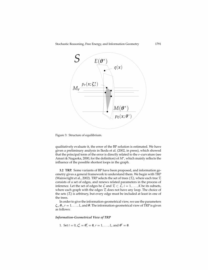
Figure 3: Structure of equilibrium.

qualitatively evaluate it, the error of the BP solution is estimated. We havegiven a preliminary analysis in Ikeda et al. (2002, in press), which showedthat the principal term of the error is directly related to the e–curvature (seeAmari & Nagaoka, 2000, for the definition) of M∗, which mainly reflects theinfluence of the possible shortest loops in the graph.

3.2 TRP. Some variants of BP have been proposed, and information ge-ometry gives a general framework to understand them. We begin with TRP(Wainwright et al., 2002). TRP selects the set of trees {Ti}, where each tree Ticonsists of a set of edges, and renews related parameters in the process ofinference. Let the set of edges be L and Ti ⊂ L, i = 1, . . . , K be its subsets,where each graph with the edges Ti does not have any loop. The choice ofthe sets {Ti} is arbitrary, but every edge must be included at least in one ofthe trees.

In order to give the information-geometrical view, we use the parametersζr,θr, r = 1, . . . , L, andθ. The information-geometrical view of TRP is givenas follows:

Information-Geometrical View of TRP

1. Set t = 0, ζtr = θt

r = 0, r = 1, . . . , L, and θt = 0.


2. For a tree Ti, construct a tree distribution ptTi

(x) as follows

ptTi

(x) = Cp0(x;θt)∏r∈Ti

pr(x; ζtr)

p0(x;θtr)

= C′ exp

{h · x +

∑r∈Ti

cr(x) +[∑

r∈Ti

(ζtr − θt

r) + θt

]· x

}. (3.6)

By applying BP, calculate the marginal distribution of ptTi

(x), and letθt+1 = πM0◦pt

Ti(x). Then update θt+1

r and ζt+1r as follows:

For r ∈ Ti,

θt+1r = θt+1

, ζt+1r = πMr◦pt

Ti(x).

For r /∈ Ti,

θt+1r = θt

r, ζt+1r = ζt

r.

3. Repeat step 2 for trees Tj ∈ {Ti}.4. Repeat steps 2 and 3 until θt+1

r = θt+1 holds for every r, and {ζt+1r }

converges.

Let us show that the e– and the m–conditions are satisfied at the equilib-rium of TRP. Since pt

Ti(x) is a tree graph, BP in step 2 gives the exact inference

of marginal distributions. Moreover, from equations 3.5 and 3.6, we have

ptTi

(x) = Cp0(x;θt)

∏r∈Ti

pr(x; ζtr)∏

r∈Tip0(x;θt

r)=

∏r∈Ti

pr(x; ζt+1r )

p0(x;θt+1)|Ti|−1

.

where |Ti| is the cardinality of Ti. By comparing the second and third termsand using θt+1

r = θt+1, r ∈ Ti,∑r∈Ti

(ζtr − θt

r) + θt =∑r∈Ti

ζt+1r − (|Ti| − 1)θt+1 =

∑r∈Ti

(ζt+1r − θt+1

r ) + θt+1.

Since∑

r/∈Ti(ζt

r −θtr) does not change through step 2, we have the following

relation, which shows that the e–condition holds for the convergent pointof TRP:∑

rζ∗

r − (L − 1)θ∗ =∑

r(ζ∗

r − θ∗r ) + θ∗ =

∑r

(ζtr − θt

r) + θt = 0.

When TRP converges, the operation of step 2 shows that each tree distribu-tion has the same marginal distribution, which shows p∗

Ti(x) ∈ M∗, where

p∗Ti

(x) is the tree distribution constructed with the converged parameters.Sinceζ∗

r = πMr◦p∗Ti

(x), r ∈ Ti holds, pr(x; ζ∗r ) ∈ M∗ also holds for r = 1, . . . , L,

which shows the m–condition is satisfied at the convergent point.


3.3 CCCP. CCCP is an iterative procedure to obtain the minimum of afunction, which is represented by the difference of two convex functions(Yuille & Rangarajan, 2003). The idea of CCCP was applied to solve theinference problem of loopy graphs, where the Bethe free energy, which wewill discuss in section 4, is the energy function (Yuille, 2002) (therefore, itis CCCP-Bethe, but in the following, we refer it as CCCP). The detail of thederivation will be given in the appendix, and CCCP is defined as follows inan information-geometrical framework.

Information-Geometrical View of CCCP

Inner loop: Given θt, calculate {ζt+1r } by solving

πM0 ◦ pr(x; ζt+1r ) = Lθt −

∑rζt+1

r , r = 1, . . . , L. (3.7)

Outer loop: Given a set of {ζt+1r } as the result of the inner loop, calculate

θt+1 = Lθt −∑

rζt+1

r . (3.8)

From equations 3.7 and 3.8, one obtains

θt+1 = πM0 ◦ pr(x; ζt+1r ), r = 1, . . . , L,

which means that CCCP enforces the m–condition at each iteration. On theother hand, the e–condition is satisfied only at the convergent point, whichcan be easily verified by letting θt+1 = θt = θ∗ in equation 3.8 to yield the e–condition (L − 1)θ∗ = ∑

r ζ∗r . One can therefore see that the inner and outer

loops of CCCP solve the m–condition and the e–condition, respectively.

4 Free Energy Function

4.1 Bethe Free Energy. We have described the information-geometricalview of BP and related algorithms. It has the characteristics of the equilib-rium points, but it is not enough to describe the approximation accuracyand the dynamics of the algorithm.

An energy function helps us to clarify them, and there are some functionsproposed for this purpose. The most popular one is the Bethe free energy.The Bethe free energy itself is well known in the literature of statisticalmechanics, being used in formulating the so-called Bethe approximation(Itzykson & Drouffe, 1989). As far as we know, Kabashima and Saad (2001)were the first to point out that BP is derived by considering a variationalextremization of a free energy. It was Yedidia et al. (2001a) who introduced tothe machine-learning community the formulation of BP based on the Bethe


free energy. Following Yedidia et al. (2001a) and using their terminology,the definition of the free energy is given as follows:

Fβ =∑

r

∑xr

br(xr) lnbr(xr)

exp[hixi + hjxj + cr(x)]

−∑

i(li − 1)

∑xi

bi(xi) lnbi(xi)

exp(hixi).

Here, xr denotes the pair of vertices included in the edge r, bi(xi)and br(xr)area belief and a pairwise belief respectively, and li is the number of neighborsof vertex i. From its definition,

∑xi

bi(xi) = 1, and∑

xrbr(xr) = 1 is satisfied.

In an information-geometrical formulation,

br(xr) = pr(xr; ζr).

And by setting

pr(xk; ζr) = p0(xk;θ), k /∈ rth edge,

the Bethe free energy becomes

Fβ =∑

r[ζr · ηr(ζr) − ψr(ζr)] − (L − 1)[θ · η0(θ) − ψ0(θ)]. (4.1)

In Yedidia et al. (2001a, 2001b) the following reducibility conditions (alsocalled the marginalization conditions) are further imposed:

bi(xi) =∑

xj

bij(xi, xj), bj(xj) =∑

xi

bij(xi, xj). (4.2)

These conditions are equivalent to the m–condition in equation 3.1, that is,ηr(ζr) = η0(θ), r = 1, . . . , L, so that every ζr is no longer an independentvariable but is dependent on θ. With these constraints, the Bethe free energyis simplified as follows:

Fβm(θ) = (L − 1)ψ0(θ) −∑

rψr(ζr(θ))

+[∑

rζr(θ) − (L − 1)θ

]· η0(θ). (4.3)

At each step of the BP algorithm, equation 4.2 is not satisfied, but the e–condition is satisfied. Therefore, assuming equation 4.2 for original BP im-mediately gives the equilibrium, and no free parameter is left. Without anyfree parameter, it is not possible to take the derivative, which does not al-low us to give any further analysis in terms of the Bethe free energy. Thus,


it is important to specify in any analysis based on the free energy what theindependent variables are, in order to provide a proper argument.

Finally, we mention the relation between the Bethe free energy and theconventional (Helmholtz) free energy ψq, the logarithm of the partition func-tion of q(x) defined in equation 2.1. When the e–condition is satisfied,Fβm(θ)

becomes

Fβm(θ) = (L − 1)ψ0(θ) −∑

rψr(ζr(θ))

= −{

ψ0(θ) +∑

r[ψr(ζr(θ)) − ψ0(θ)]

}.

This formula shows that the Bethe free energy can be regarded as an ap-proximation to the conventional free energy by a linear combination of ψ0and {ψr}. Moreover, if the graph is a tree, the result of proposition 1 showsthat the Bethe free energy is equivalent to −ψq.

4.2 A New View on Free Energy. Instead of assuming equation 4.2, letus start from the free energy defined in equation 4.3 without any constrainton the parameters; that is, all of θ, ζ1, . . . , ζL are the free parameters:

F(θ, ζ1, . . . , ζL) = (L − 1)ψ0(θ) −∑

rψr(ζr)

+[∑

rζr − (L − 1)θ

]· η0(θ). (4.4)

The above function is rewritten in terms of the KL divergence as

F(θ, ζ1, . . . , ζL) = D[p0(x;θ); q(x)] −∑

rD[p0(x;θ); pr(x; ζr)] + C,

where C is a constant. The following theorem is easily derived.

Theorem 3. The equilibrium (θ∗, ζ∗

r ) of BP is a critical point of F(θ, ζ1, . . . ,

ζr).

Proof. By calculating

∂F∂ζr

= 0,

we easily have

ηr(ζr) = η0(θ),


which is the m–condition. By calculating

∂F∂θ

= 0, (4.5)

we are led to the e–condition (L − 1)θ = ∑r ζr.

The theorem shows that equation 4.4 works as the free energy functionwithout any constraint.

4.3 Relation to Other Free Energies. The function F(θ, ζ1, . . . , ζL)

works as a free energy function, but it is also important to compare itwith other “free energies.” First, we compare it with the one proposed byKabashima and Saad (2001). It is a function of (ζ1, . . . , ζL) and (ξ1, . . . , ξL),given by

FKS(ζ1, . . . , ζL; ξ1, . . . , ξL) = F(θ, ζ1, . . . , ζL)

+∑

rD[p0(x;θ); p0(x; ζr + ξr)],

where θ = ∑r ξr. It is clear from the definition that the choice of ξr that

makes FKS minimum is ξr = θ − ζr, for all r, and FKS becomes equivalentto F .

Next, we consider the dual form of the free energy Fβ in equation 4.1.The dual form is defined by introducing the Lagrange multipliers (Yedidiaet al., 2001a) and redefining the free energy as a function of them. Themultipliers are defined on the reducibility conditions, bi(xi) = ∑

xjbij(xi, xj)

and bj(xj) = ∑xi

bij(xi, xj). They are equivalent to ηr(ζr) = η0(θ), whichis the m–condition in information-geometrical formulation. Let λr ∈ �n,r = 1, . . . , L be the Lagrange multipliers, and the free energy becomes

G(θ, {ζr}, {λr}) = Fβ(θ, {ζr}) −∑

rλr · [ηr(ζr) − η0(θ)], λr ∈ �n.

The original extremal problem is equivalent to the extremal problem of Gwith respect to θ, {ζr}, and {λr}. The dual formGβ is derived by redefiningGas a function of {λr}, where the extremal problems of θ and {ζr} are solved.By solving ∂θG = 0, we have

θ({λr}) = 1L − 1

∑rλr,

while ∂ζrG = 0 gives

ζr(λr) = λr.


Finally, the dual form Gβ becomes

Gβ({λr}) = (L − 1)ψ0(θ({λr})) −∑

rψr(ζr(λr)). (4.6)

Although F in equation 4.4 becomes equivalent to Gβ by assuming the e–condition, F is free from the e– and the m–conditions and is different fromGβ .

From the definition of the Lagrange multipliers, Gβ is introduced to an-alyze the extremal problem of Fβ under the m–condition, where the e–condition is not satisfied. The m–constraint free energy Fβm in equation 4.3shows that F is equivalent to Fβ under the m–condition.

Finally, we summarize as follows: Under the m–condition,F is equivalentto Fβ , and under the e–condition, F is equivalent to the dual form Gβ .

4.4 Property of Fixed Points. Let us study the stability of the fixed pointof Fβ or, equivalently, F under the m–condition. Since the m–conditionis satisfied, every ζr is a dependent variable of θ, and we consider thederivative with respect to θ. From the m–condition, we have

ηr(ζr) = η0(θ),∂ζr

∂θ= I−1

r (ζr)I0(θ), r = 1, . . . , L. (4.7)

Here, I0(θ) and Ir(ζr) are the Fisher information matrices of p0(x;θ) andpr(x; ζr), respectively, which are defined as

I0(ζr) = ∂θη0(θ) = ∂2θψ0(θ), Ir(ζr) = ∂ζrηr(ζr) = ∂2

ζrψr(ζr),

r = 1, . . . , L.

Equation 4.7 is proved as follows:

ηr(ζr) + Ir(ζr)δζr ηr(ζr + δζr) = η0(θ + δθ) η0(θ) + I0(θ)δθ

δζr = Ir(ζr)−1I0(θ)δθ. (4.8)

The condition of the equilibrium is equation 4.5 which yields the e–condition,and the second derivative gives the property around the stationary point,that is,

∂2F∂θ2 = I0(θ) + I0(θ)

∑r

[Ir(ζr)−1 − I0(θ)−1]I0(θ) + , (4.9)

where is the term related to the derivative of the Fisher information matrix,which vanishes when the e–condition is satisfied.

If equation 4.9 is positive definite at the stationary point, the Bethe freeenergy is at least locally minimized at the equilibrium. But it is not alwayspositive definite. Therefore, the conventional gradient descent method ofFβ or F may fail.


5 Algorithms and Their Convergences

5.1 e–constraint Algorithm. Since the equilibrium of BP is characterizedwith the e– and the m–conditions, there are two possible algorithms forfinding the equilibrium. One is to constrain the parameters always to satisfythe e–condition and search for the parameters that satisfy the m–condition(e–constraint algorithm). The other is to constrain the parameters to satisfythe m–condition and search for the parameters that satisfy the e–condition(m–constraint algorithm).

In this section, we discuss e–constraint algorithms. BP is an e–constraintalgorithm since the e–condition is satisfied at each step, but its convergenceis not necessarily guaranteed. We give an alternative of the e–constraint al-gorithm that has a better convergence property. Let us begin with proposinga new cost function as

Fe({ζr}) =∑

r||η0(θ)−ηr(ζr)||2, (5.1)

under the e–constraint θ = ∑r ζr/(L − 1). If the cost function is minimized

to 0, the m–condition is satisfied, and it is an equilibrium. A naive methodto minimize Fe is the gradient descent algorithm. The gradient is

∂Fe

∂ζr= −2Ir(ζr)[η0(θ)−ηr(ζr)] + 2

L − 1I0(θ)

∑r

[η0(θ)−ηr(ζr)]. (5.2)

If the derivative is available, ζr and θ are updated as

ζt+1r = ζt

r − δ∂Fe

∂ζtr

, θt+1 = 1L

∑rζt+1

r ,

where δ is a small positive learning rate. It is not difficult to calculate η0(θ),ηr(ζr), and I0(θ), and the rest of the problem is to calculate the first term ofequation 5.2. Fortunately, we have the relation,

Ir(ζr)h = limα→0

ηr(ζr + αh) − ηr(ζr)

α.

If (η0(θ)−ηr(ζr)) is substituted for h, this becomes the first term of equa-tion 5.2. Now we propose a new algorithm.

A New e–Constraint Algorithm

1. Set t = 0, θt = 0, ζtr = 0, r = 1, . . . , L.

2. Calculate η0(θt), I0(θ

t), and ηr(ζ

tr), r = 1, . . . , L.

3. Let hr=η0(θt)−ηr(ζ

tr)and calculateηr(ζ

tr+αhr) for r = 1, . . . , L, where

α>0 is small. Then calculate

gr = ηr(ζtr + αh) − ηr(ζ

tr)

α.


4. For t = 1, 2, . . . , update ζt+1r as follows:

ζt+1r = ζt

r − δ

[−2gr + 2

L − 1I0(θ

t)∑

rhr

],

θt+1 = 1L − 1

∑rζt+1

r .

5. If Fe({ζr}) = ∑r ||η0(θ)−ηr(ζr)||2 > ε (ε is a threshold) holds, t+1→t

and go to 2.

This algorithm is an e–constraint algorithm and does not include dou-ble loops, which is similar to the BP algorithm, but we have introduceda new parameter α, which can affect the convergence. We have checked,with small-sized numerical simulations, that if α is sufficiently small, thisproblem can be avoided, but further theoretical analysis is needed. Anotherproblem is that this algorithm converges to any fixed point of BP even if itis not a stable fixed point of BP. For example, when ζr and θ are extremelylarge, eventually every component of ηr and η0 becomes close to 1, whichis a trivial useless fixed point of this algorithm. In order to avoid this, it isnatural to use the Riemannian metric for the norm instead of the squarenorm defined in equation 5.1. The local metric modifies the cost function to

FeR({ζr}) =∑

r[η0(θ) − ηr(ζr)]

TI0(θ0)−1[η0(θ) − ηr(ζr)],

where θ0 is the convergent point. Since I0(θ0)−1 diverges at the trivial fixed

points mentioned above, we expect FeR({ζr}) to be a better cost function.The gradient can be calculated similarly by fixing θ0, which is unknown.Hence, we replace it by θt. The calculation of gr should also be modified to

g̃r = ηr(ζtr + αI0(θ

t)−1 ∑

r hr)

α

from the point of view of the natural gradient method (Amari, 1998). Wefinally have

ζt+1r = ζt

r − 2δI0(θt)−1

[−g̃r + 1

L − 1

∑r

hr

].

Since I0(θ) is a diagonal matrix, computation is simple.

5.2 m–constraint Algorithm. The other possibility is to constrain theparameters always to satisfy the m–condition and modify the parameters tosatisfy the e–condition. Since the m–condition is satisfied, {ζr} are dependenton θ.


A naive idea is to repeat the following two steps:

Naive m–Constraint Algorithm

1. For r = 1, . . . , L,

ζtr = πMr ◦ p0(x;θt

). (5.3)

2. Update the parameters as

θt+1 = Lθt −∑

rζt

r.

Starting from θt, the algorithm finds {ζt+1r } that satisfies the m–condition

by equation 5.3, and θt+1 is adjusted to satisfy the e–condition.This is a simple recursive algorithm without double loops. We call it the

naive m–constraint algorithm. One may use an advanced iteration methodthat uses new ζt+1

r instead of ζtr. In this case, the algorithm is

ζt+1r = πMr ◦ p0(x;θt+1

), where θt+1 = Lθt −∑

rζt+1

r .

In this algorithm, starting from θt, one should solve a nonlinear equationin θt+1, because {ζt+1

r } are functions of θt+1. This algorithm therefore usesdouble loops—the inner loop and the outer loop. This is the idea of CCCP,and it is also an m–constraint algorithm.

5.2.1 Stability of the Algorithms. Although the naive m–constraint algo-rithm and CCCP share the same equilibrium θ∗ and {ζ∗

r }, their local stabil-ities at the equilibrium are different. It is reported that CCCP has superiorproperties in this respect. The local stability of BP was analyzed by Richard-son (2000) and also by Ikeda et al. (in press) in geometrical terms. Thestability condition of BP is given by the conditions of the eigenvalues of amatrix defined by the Fisher information matrices. In this article, we givethe local stability of the other algorithms.

If we eliminate the intermediate variables {ζr} in the inner loop, the naivem–constraint algorithm is

θt+1 = Lθt −∑

rπMr ◦ p0(x;θt

), (5.4)

and CCCP is represented as

θt+1 = Lθt −∑

rπMr ◦ p0(x;θt+1

). (5.5)

In order to derive the variational equation at the equilibrium, we note thatfor the m–projection,

ζr = πMr ◦ p0(x;θ),


a small perturbation δθ in θ is updated as

δζr = Ir(ζr)−1I0(θ)δθ

(see equation 4.8). The variational equations are hence for equation 5.4,

δθt+1 =[

LE −∑

rIr(ζr)

−1I0(θ)

]δθt

,

where E is the identity matrix, and for equation 5.5,

δθt+1 = L

[E +

∑r

Ir(ζr)−1I0(θ)

]−1

δθt,

respectively. Let K be a matrix defined by

K = 1L

∑r

√I0(θ)Ir(ζr)

−1√

I0(θ)

and δθ̃t

be a new variable defined as

δθ̃t =

√I0(θ)δθt

.

The variational equations for equations 5.4 and 5.5 are then

δθ̃t+1 = L(E − LK)δθ̃

t,

δθ̃t+1 = L(E + LK)−1δθ̃

t,

respectively.The equilibrium is stable when the absolute values of the eigenvalues

of the respective coefficient matrices are smaller than 1. Let λ1, . . . , λn bethe eigenvalues of K. They are all real and positive, since K is a symmetricpositive-definite matrix. We note that λi are close to 1, when Ir(ζr) ≈ I0(θ)

or Mr is close to M0. The following theorem shows that CCCP has a goodconvergent property.

Theorem 4. The equilibrium of the naive m–constraint algorithm in equation 5.4is stable when

1 + 1L

> λi > 1 − 1L

, i = 1, . . . , n.

The equilibrium of CCCP is stable when the eigenvalues of K satisfy

λi > 1 − 1L

, i = 1, . . . , n. (5.6)


Under the m–constraint, the Hessian ofF(θ) at an equilibrium point is equalto (cf. equation 4.9)√

I0(θ)[LK − (L − 1)E]√

I0(θ),

so that the stability condition (see equation 5.6) for CCCP is equivalentto the condition that the equilibrium is a local minimum of F under them–constraint, which is equivalent to the m–constraint Bethe free energyFβm(θ). The theorem therefore states that CCCP is locally stable around anequilibrium if and only if the equilibrium is a local minimum of Fβm(θ),whereas the naive m–constraint algorithm is not necessarily stable even ifthe equilibrium is a local minimum. A similar result is obtained in Heskes(2003).

It should be noted that the above local stability result for CCCP does notfollow from the global convergence result given by Yuille (2002). Yuille hasshown that CCCP decreases the cost function and converges to an extremalpoint of Fβm(θ), which means the fixed point is not necessarily a localminimum but can be a saddle point. Our local linear analysis shows that astable fixed point of CCCP is a local minimum of Fβm(θ).

5.2.2 Natural Gradient and Discretization. Let us consider a gradient rulefor updating θ to find a minimum of F under the m–condition

θ̇ = −∂F(θ)

∂θ.

When we have a metric to measure the distance in the space of θ, it isnatural to use the metric for gradient (natural gradient; see Amari, 1998). Forstatistical models, the Riemannian metric given by the Fisher informationmatrix is a natural choice, since it is derived from KL divergence. The naturalgradient version of the update rule is

θ̇ = −I−10 (θ)

∂F∂θ

= (L − 1)θ −∑

rπMr ◦ p0(x;θ). (5.7)

For the implementation, it is necessary to discretize the continuous-timeupdate rule. The “fully explicit” scheme of discretization (Euler’s method)reads

θt+1 = θt + t

[(L − 1)θt −

∑r

πMr ◦ p0(x;θt)

]. (5.8)

When t = 1, this is equivalent to the naive m–constraint algorithm (seeequation 5.4). However, we do not necessarily have to let t = 1. Instead, wemay use arbitrary positive value for t. We will show how the convergencerate will be affected by the change of t later.


The “fully implicit” scheme yields

θt+1 = θt + t

[(L − 1)θt+1 −

∑r

πMr ◦ p0(x;θt+1)

], (5.9)

which, after rearrangement of terms, becomes

[1 − t(L − 1)]θt+1 = θt − t∑

rπMr ◦ p0(x;θt+1

).

When t = 1/L, this equation is equivalent to CCCP in equation 5.5. Again,we do not have to be bound to the choice t = 1/L. We will also show therelation between t and the convergence rate later.

We have just shown that the naive m–constraint algorithm and CCCP canbe viewed as first-order methods of discretization applied to the continuous-time natural gradient system shown in equation 5.7. The local stability resultfor CCCP proved in theorem 4 can also be understood as an example of thewell-known absolute stability property of the fully implicit scheme appliedto linear systems. It should also be noted that other more sophisticatedmethods for solving ordinary differential equations, such as Runge-Kuttamethods (possibly with adaptive step-size control) and the Bulirsch-Stoermethod Press, Teukolsky, Vetterling, and Flannery (1992), are applicable forformulating m–constraint algorithms with better properties, for example,better stability. In this article, however, we do not discuss possible extensionalong this line any further.

5.2.3 Acceleration of m–Constraint Algorithms. We give the analysis ofequations 5.8 and 5.9 in this section.

The variational equation for equation 5.8 is

δθ̃t+1 = {E − [LK − (L − 1)E] t}δθ̃t

.

Let

λ1 ≤ λ2 ≤ · · · ≤ λn (5.10)

be the eigenvalues of K. Then the convergence rate is improved by choosingan adequate t. The convergence rate is governed by the largest absolutevalues of the eigenvalues of E − [LK − (L − 1)E] t, which are given by

µi = 1 − [Lλi − (L − 1)] t.

From equation 5.10, we have µ1 ≥ µ2 ≥ · · · ≥ µn. The stability condition is|µi| < 1 for all i. At a locally stable equilibrium point, µ1 < 1 always holds,so that the algorithm is stable if µn > −1 holds. The convergence to a locally


stable equilibrium point is most accelerated when µ1 +µn = 0, which holdsby taking

topt = 2L(λ1 + λn − 1) + 2

.

The variational equation for equation 5.9 is

δθ̃t+1 = {E + [LK − (L − 1)E] t}−1δθ̃

t,

and the convergence rate is governed by the largest of the absolute valuesof the eigenvalues of {E + [LK − (L − 1)E] t}−1, which should be smallerthan 1 for convergence. The eigenvalues are

µi = 11 + [Lλi − (L − 1)] t

.

We again have µ1 ≥ µ2 ≥ · · · ≥ µn. At a locally stable equilibrium point,0 < µn and µ1 < 1 always hold, so that the algorithm is always stable. Inprinciple, the smaller µ1 becomes, the faster the algorithm converges, so thattaking t → +∞ yields the fastest convergence. However, the algorithmin this limit reduces to the direct evaluation of the e–condition under them–constraint with one update step of the parameters. This is the fastest if itis possible, but this is usually infeasible for loopy graphs.

6 Extension

6.1 Extend the Framework to Wider Class of Distributions. In this sec-tion, two important extensions of BP are given in the information-geomet-rical framework. First, we extend the model to the case where the marginaldistribution of each vertex is an exponential family. A similar extension isgiven in Wainwright, Jaakola, and Willsky (2003).

Let ti be the sufficient statistics of the marginal distribution of xi, that is,q(xi). The marginal distribution is in the family of distributions defined asfollows:

p(xi;θi) = exp[θi · ti − ϕi(θi)].

This includes many important distributions. For example, multinomial dis-tribution and gaussian distribution are included in this family.

Let us define t = (tT1 , . . . , tT

n )T and θ = (θT1 , . . . ,θT

n)T, and let the truedistribution be

q(x) = exp[h · t + c(x) − ψq].

We can now redefine equation 2.2 as follows,

p(x;θ, v) = exp[θ · t + v · c(x) − ψ(θ, v)],


and S in equation 2.3 as

S = {p(x;θ, v) | θ ∈ �, v ∈ V}.

When the problem is to infer the marginal distribution q(xi) of q(x), wecan redefine the BP algorithm in this new S by redefining M0 and Mr. Thisextension based on the new definition is simple, and we do not give furtherdetails in this article.

6.2 Generalized Belief Propagation. In this section, we show the infor-mation-geometrical framework for the general belief propagation (GBP;Yedidia et al., 2001b), which is an important extension of BP.

A naive explanation of GBP is that the cliques are reformulated by subsetsof L, which is the set of all the edges. This brings us a new implementationof the algorithm and a different inference. In the information-geometricalformulation, we define c′

s(x) as a new clique function, which summarizesthe interactions of the edges in Ls, s = 1, . . . , L′, that is,

c′s(x) =

∑r∈Ls

cr(x),

where Ls ⊆ L. Those Ls may have overlaps, and Ls must be chosen tosatisfy ∪sLs = L.

GBP is a general framework, which includes a lot of possible cases.We categorize them into three important classes and give an information-geometrical framework for them:

Case 1. In the simplest case, each Ls does not have any loop. This isequivalent to TRP. As we saw in section 3.2, the algorithm is explained inthe information-geometrical framework.

Case 2. In this case, eachLs can have loops, but there is no overlap, thatis, Ls ∩ Ls′ = ∅ for s �= s′. The extension to this case is also simple. We canapply information geometry by redefining Mr as Ms, where its definition isgiven as

Ms = {ps(x; ζs) = exp[h · x + c′s(x) + ζs · x − ψs(ζs)] | ζs ∈ �n}.

Since some loops are treated in a different way, the result might be differentfrom BP.

Case 3. Finally, we describe the case where each Ls can have loops andoverlaps with the other sets. In this case, we have to extend the framework.Suppose Ls and Ls′ have an overlap, and both have loops. We explain thecase with an example in Figure 4.


x1

x2

x3

x4

1

23

4

5

Figure 4: Case 3.

Let us first define the following distributions:

q(x) = exp

[h · x +

5∑i=1

ci(x) − ψq

]

p0(x;θ) = exp[h · x + θ · x − ψ0(θ)] (6.1)

p1(x; ζ1) = exp

[h · x +

3∑i=1

ci(x) + ζ1 · x − ψ1(ζ1)

](6.2)

p2(x; ζ2) = exp

[h · x +

5∑i=3

ci(x) + ζ2 · x − ψ2(ζ2)

]. (6.3)

Even if ζ1, ζ2, and θ satisfy the e–condition as θ = ζ1 + ζ2, this does notimply that

Cp1(x; ζ1)p2(x; ζ2)

p0(x;θ)

is equivalent to q(x), since c3(x) is counted twice. Therefore, we introduceanother model p3(x; ζ3), which has the following form:

p3(x; ζ3) = exp[h · x + c3(x) + ζ3 · x − ψ3(ζ3)]. (6.4)

Now,

Cp1(x; ζ1)p2(x; ζ2)

p3(x; ζ3)

becomes equal to q(x), where ζ3 = ζ1 + ζ2 is the e–condition.Next, we look at the m–condition. The original form of the m–condition

is ∑x

xp0(x;θ) =∑x

xps(x; ζs),


but in this case, this form is not enough. We need a further condition, thatis,

ps(x2, x3; ζs) =∑x1,x4

ps(x; ζs)

should be the same for s = {1, 2, 3}. The models in equations 6.1, 6.2, 6.3, and6.4 are not sufficient, since we do not have enough parameters to specify ajoint distribution of (x2, x3), and the model must be extended. In the binarycase, we can extend the models by adding one variable as follows:

p1(x; ζ1, v1) = exp

[h · x +

3∑i=1

ci(x) + ζ1 · x + v1x2x3 − ψ1(ζ1, v1)

]

p2(x; ζ2, v2) = exp

[h · x +

5∑i=3

ci(x) + ζ2 · x + v2x2x3 − ψ2(ζ2, v2)

]

p3(x; ζ3, v3) = exp[h · x + c3(x) + ζ3 · x + v3x2x3 − ψ3(ζ3, v3)],

and the m–condition becomes∑x

xp0(x;θ) =∑x

xps(x; ζs, vs), s = 1, 2, 3,

∑x

x2x3p1(x; ζ1, v1) =∑x

x2x3p2(x; ζ2, v2) =∑x

x2x3p3(x; ζ3, v3).

We revisit the e–condition, which is now extended as

ζ3 = ζ1 + ζ2, v3 = v1 + v2.

This is a simple example, but we can describe any GBP problem in theinformation-geometrical framework in a similar way.

7 Conclusion

Stochastic reasoning is an important technique widely used for graphicalmodels with many interesting applications. BP is a useful method to solveit, and in order to analyze its behavior and give a theoretical foundation,a variety of approaches have been proposed from AI, statistical physics,information theory, and information geometry. We have shown a unifiedframework for understanding various interdisciplinary concepts and algo-rithms from the point of view of information geometry. Since informationgeometry captures the essential structure of the manifold of probability dis-tributions, we are successful in clarifying the intrinsic geometrical structuresand their difference of various algorithms proposed so far.

The BP solution is characterized with the e– and the m–conditions. Wehave shown that BP and TRP explore the solution in the subspace where the


e–condition is satisfied, while CCCP does so in the subspace where the m–condition is satisfied. This analysis makes it possible to obtain new, efficientvariants of these algorithms. We have proposed new e– and m–constraint al-gorithms. The possible acceleration methods for the m–constraint algorithmand CCCP are shown with local stability and convergence rate analysis. Wehave clarified the relation among the free-energy-like functions and haveproposed a new one. Finally, we have shown possible extensions of BP froman information-geometrical viewpoint.

This work is a first step toward an information-geometrical understand-ing of BP. By using this framework, we expect further understanding and anew improvement of the methods will emerge.

Appendix: Information-Geometrical View of CCCP

In this section, we derive the information-geometrical view of CCCP. Thefollowing two theorems play important roles in CCCP.

Theorem 5 (Yuille & Rangarajan, 2003, sect. 2). Let E(x) be an energy func-tion with bounded Hessian ∂E2(x)/∂x∂x. Then we can always decompose it intothe sum of a convex function and a concave function.

Theorem 6 (Yuille & Rangarajan, 2003, sect. 2). Consider an energy functionE(x) (bounded below) of form E(x) = Evex(x)+Ecave(x) where Evex(x), Ecave(x) areconvex and concave functions of x, respectively. Then the discrete iterative CCCPalgorithm xt �→ xt+1 given by

∇Evex(xt+1) = −∇Ecave(xt)

is guaranteed to monotonically decrease the energy E(x) as a function of time andhence to converge to a minimum or saddle point of E(x) (or even a local maximumif it starts at one).

The idea of CCCP was applied to solve the inference problem of loopygraphs, where the Bethe free energyFβ in equation 4.1 is the energy function(Yuille, 2002). The concave and convex functions are defined as follows:

Fβ(θ, {ζr}) =∑

r[ζr · ηr(ζr) − ψr(ζr)] − (L − 1)[θ · η0(θ) − ψ0(θ)]

= Fvex(θ, {ζr}) + Fcave(θ, {ζr})Fvex(θ, {ζr}) =

∑r

[ζr · ηr(ζr) − ψr(ζr)] + [θ · η0(θ) − ψ0(θ)],

Fcave(θ) = −L[θ · η0(θ) − ψ0(θ)].

Let the m–condition be satisfied, and Fvex is a function of θ. Next, sinceη0 and θ have a one-to-one relation, let η0 be the coordinate system. The


gradient of Fvex and Fcave is given as

∇η0Fvex(η0) = θ +∑

rζr, −∇η0Fcave(η0) = Lθ.

Finally, the CCCP algorithm is written as

∇η0Fvex(ηt+10 ) = −∇η0Fcave(η

t0)

θt+1 +∑

rζt+1

r = Lθt. (A.1)

Since the m–condition is not satisfied in general, the inner loop solves thecondition, while the outer loop updates the parameters as equation A.1.

Acknowledgments

We thank the anonymous reviewers for valuable feedback. This work wassupported by the Grant-in-Aid for Scientific Research 14084208 and14084209, MEXT, Japan and 14654017, JSPS, Japan.

References

Amari, S. (1998). Natural gradient works efficiently in learning. Neural Compu-tation, 10, 251–276.

Amari, S. (2001). Information geometry on hierarchy of probability distributions.IEEE Trans. Information Theory, 47, 1701–1711.

Amari, S., Ikeda, S., & Shimokawa, H. (2001). Information geometry and meanfield approximation: The α-projection approach. In M. Opper & D. Saad(Eds.), Advanced mean field methods—Theory and practice (pp. 241–257). Cam-bridge, MA: MIT Press.

Amari, S., & Nagaoka, H. (2000). Methods of information geometry. Providence,RI: AMS, and New York: Oxford University Press.

Heskes, T. (2003). Stable fixed points of loopy belief propagation are minima ofthe Bethe free energy. In S. Becker, S. Thrun, & K. Obermayer (Eds.), Advancesin neural information processing systems, 15 (pp. 359–366). Cambridge, MA: MITPress.

Ikeda, S., Tanaka, T., & Amari, S. (2002). Information geometrical frameworkfor analyzing belief propagation decoder. In T. G. Dietterich, S. Becker, &Z. Ghahramani (Eds.), Advances in neural information processing systems, 14(pp. 407–414). Cambridge, MA: MIT Press.

Ikeda, S., Tanaka, T., & Amari, S. (in press). Information geometry of turbo codesand low-density parity-check codes. IEEE Trans. Information Theory.

Itzykson, C. & Drouffe, J.-M. (1989). Statistical field theory. Cambridge: Cam-bridge University Press.

Jordan, M. I. (1999). Learning in graphical models. Cambridge, MA: MIT Press.Kabashima, Y., & Saad, D. (1999). Statistical mechanics of error-correcting codes.

Europhysics Letters, 45, 97–103.


Kabashima, Y., & Saad, D. (2001). The TAP approach to intensive and extensiveconnectivity systems. In M. Opper & D. Saad (Eds.), Advanced mean fieldmethods—Theory and practice (pp. 65–84). Cambridge, MA: MIT Press.

Lauritzen, S. L., & Spiegelhalter, D. J. (1988). Local computations with probabil-ities on graphical structures and their application to expert systems. Journalof the Royal Statistical Society B, 50, 157–224.

Pearl, J. (1988). Probabilistic reasoning in intelligent systems: Networks of plausibleinference. San Mateo, CA: Morgan Kaufmann.

Press, W. H., Teukolsky, S. A., Vetterling, W. T., & Flannery, B. P. (1992). Numericalrecipes in C: The art of scientific computing. Cambridge: Cambridge UniversityPress.

Richardson, T. J. (2000). The geometry of turbo-decoding dynamics. IEEE Trans.Information Theory, 46, 9–23.

Tanaka, T. (2000). Information geometry of mean-field approximation. NeuralComputation, 12, 1951–1968.

Tanaka, T. (2001). Information geometry of mean-field approximation. In M. Op-per & D. Saad (Eds.), Advanced mean field methods—Theory and practice (pp.259–273). Cambridge, MA: MIT Press.

Wainwright, M., Jaakkola, T., & Willsky, A. (2002). Tree-based reparameteriza-tion for approximate inference on loopy graphs. In T. G. Dietterich, S. Becker,& Z. Ghahramani (Eds.), Advances in neural information processing systems, 14(pp. 1001–1008). Cambridge, MA: MIT Press.

Wainwright, M., Jaakkola, T., & Willsky, A. (2003). Tree-reweighted beliefpropagation algorithms and approximate ML estimate by pseudo-momentmatching. In C. M. Bishop & B. J. Frey (Eds.), Proceedings of Ninth Inter-national Workshop on Artificial Intelligence and Statistics. Available on-line at:http://www.research.microsoft.com/conferences/aistats2003/.

Weiss, Y. (2000). Correctness of local probability propagation in graphical modelswith loops. Neural Computation, 12, 1–41.

Yedidia, J. S., Freeman, W. T., & Weiss, Y. (2001a). Bethe free energy, Kikuchiapproximations, and belief propagation algorithms (Tech. Rep. No. TR2001–16).Cambridge, MA: Mitsubishi Electric Research Laboratories.

Yedidia, J. S., Freeman, W. T., & Weiss, Y. (2001b). Generalized belief propagation.In T. K. Leen, T. G. Dietterich, & V. Tresp (Eds.), Advances in neural informationprocessing systems, 13 (pp. 689–695). Cambridge, MA: MIT Press.

Yuille, A. L. (2002). CCCP algorithms to minimize the Bethe and Kikuchi freeenergies: Convergent alternatives to belief propagation. Neural Computation,14, 1691–1722.

Yuille, A. L., & Rangarajan, A. (2003). The concave-convex procedure. NeuralComputation, 15, 915–936.

Received August 12, 2003; accepted March 3, 2004.

stochastic reasoning, free energy, and...

Documents