Stochastic Simulation and Monte Carlo

Methods

Andreas Hellander

March 31, 2009

1 Stochastic models, Stochastic methods

In these lecture notes we will work through three different computationalproblems from different application areas. We will simulate the irregularmotion of a particle in an environment of smaller solvent molecules, we willstudy a biochemical control network and we will compute a numerical approx-imation to a high dimensional integral. Even though these three problemsare different, and the way we will solve them will be different, they have onething in common. In each case we will use a Monte Carlo method.

There is not a single definition of a Monte Carlo method, but they havein common that they make use of random sampling to compute the result.The algorithms typically rely on pseudo random numbers, computer gener-ated numbers mimicking true random numbers, to generate a realization,one possible outcome of a process. All outcomes do not have to be equallyprobable, and by repeating the procedure with different random numbers asinput, one gathers data corresponding to the modeled process. On this data,one may then perform a statistical analysis in order to answer different ques-tions about the process. We illustrate the general principle in the followingexample, which we will study in more detail using a computer in Exercise 8.

1. We have a model of some physical phenomena and some question re-garding the system we are modeling we like to answer. For example,suppose that we model the motion of a single large protein in a sur-rounding of water molecules and that the system is confined to a boxof some fixed size. Suppose we want to know the average time untilthe particle hits one of the sides of the box if it starts in the center.

2. The model is stochastic by construction, and one possible path of theparticle can be generated by a simple algorithm that repeatedly gen-

1

erates pseudo random numbers from the standard normal distribution.This means that if we generate a number of paths, they will all be dif-ferent. In order to answer the question, we use the simple algorithm togenerate many different realizations, say 105, and for each realizationwe measure and store the time it took until the particle hit one of thesides.

3. Once we have gathered the data set, the different hitting times in thiscase, we simply compute the arithmetic mean in order to get an ap-proximation of the average time.

In the following, we will make a clear distinction between stochastic mod-els and stochastic methods. For our particle example above, the model isstochastic, but in order to answer the question regarding the hitting time wecould have used a deterministic method. We can formulate a partial differ-ential equation (PDE), which if we solve it gives precisely the average timeuntil the particle leaves the box. If we used this approach, the method wouldno longer be a Monte Carlo method, but the model would still be stochastic.However, it may be much harder to solve the PDE than to repeatedly samplethe process in a Monte Carlo method, in particular if the motion takes placein higher dimensions.

A classical use of a Monte Carlo method to solve a deterministic problemis to evaluate definite integrals. Even in this case, the methodology followsthe same basic principle as in the above example. Here, the ’model’ is anintegral, and it is solved by repeatedly ’sampling’ the integrand assumingthat the independent variable is distributed according to some probabilitydistribution. In this way, we collect data and by identifying the integral witha certain expected value we can approximate it by computing the arithmeticmean of the data. The procedure is summarized below and why this methodworks will be explained in Section 3. Note the similarity with the three stepsin the particle motion problem above.

1. Suppose we want to compute the value of the integral I =∫

Ωf(x)dx

over some domain Ω.

2. We generate a data set made up of the function f evaluated at randompoints x distributed uniformly in Ω. These points are generated usinga pseudo random number generator.

3. We compute an approximation to I by computing the arithmetic meanof the data gathered in the previous step and multiplying the resultwith the volume of Ω.

2

In this case, the underlying problem is deterministic, and the use of MonteCarlo to solve it is motivated by the fact that for very high dimensions,especially for non-smooth integrands, it is more computationally efficientto solve it with MC than using a traditional quadrature rule (rememberScientific Computing I). In this example, we use a stochastic method to solvea deterministic problem for efficiency reasons.

In summary, Monte Carlo methods can be used to study both determin-istic and stochastic problems. For a stochastic model, it is often natural andeasy to come up with a stochastic simulation strategy due to the stochasticnature of the model, but depending on the question asked a deterministicmethod may be used. The use of a stochastic method is often motivatedby the fact that a deterministic method to answer the same question is notavailable, that it is is too complicated to be practically useful, or that it iscomputationally intractable, which is often the case if the problem is highdimensional. On the other hand, when a deterministic method is applica-ble, it is often preferable due to the very slow convergence of Monte Carlomethods.

No matter the reason for using Monte Carlo methods, they will inevitablyrequire many random numbers. The quality of the pseudo random genera-tors is crucial to the correctness of the results computed with a stochasticalgorithm, and the speed with which they are generated is vital to the per-formance of the stochastic method. There are many different algorithms inuse to generate pseudo random numbers, and the development of even moreefficient algorithms is an active field of research. Many courses on computa-tional statistics and Monte Carlo discusses the most basic algorithms. Wewill not do this here, since we will focus on Monte Carlo methodology ata more basic level. However, all major programming languages have someroutine for generating pseudo random numbers from (at least) the uniformdistribution, and there are many other generators freely available for noncommercial use. In the sections that follow, we will see examples of how wecan use such an ’black box’ routine to obtain random numbers from otherdistributions that we will need.

2 Two important theorems

In the following we will assume familiarity with standard statistical conceptssuch as expected value, variance and probability distribution. These notionsmay be reviewed in the course book [1]. In addition, Monte Carlo reliesheavily on two famous theorems from probability theory, namely the law oflarge numbers (LLN) and the central limit theorem (CLS) which we will state

3

without proof. If you are familiar with these theorems, you may skip thissection. They will not be explicitly needed in order to work through theexamples in the following sections, but they are required in order to reallyunderstand why MC works. If it seems artificial to you at this time, you maywant to come back to this section after reading the case studies.

Every time we estimate some unknown quantity by generating a sample(the data set composed of the realizations we generate) and computing thesample average as we will do when we evaluate integrals with Monte Carlo,we rely on the law of large numbers. Even if you have not seen the theorembefore, you have probably used it many times, especially if you have takensome experimental courses. It states that if we repeatedly sample a stochasticvariable, the sample mean converges to the true expected value. Looselyspeaking, this result says that the Monte Carlo method is consistent.

Theorem 1 (weak) Law of large numbers (LLN)

Let X1, X2, . . . , Xn be independent random variables with mean µ and setXn = 1

n

∑ni=1 Xi. Then P (Xn − δ < µ < Xn + δ) → 1 as n → ∞ for any

δ > 0.

Computer exercise 1

Implement a small Matlab routine that simulates throws with a dice. Foreach successive throw, compute the arithmetic mean based on all throws sofar and plot it as a function of N , the number of throws. To which valuedoes the mean appear to converge?

The LLN provides us with consistency, but does not give any informationregarding the error in the approximation or the rate of convergence to thetrue expected value. This is taken care of by the central limit theorem.

Theorem 2 Central limit theorem (CLS)

Let X1, X2, . . . , Xn be a sequence of independent identically distributed ran-dom variables with finite mean µ and variance σ2 > 0 and let Xn = 1

n

∑ni=1 Xi.

Then√

n(Xn − µ)D−→ N(0, σ2) as n → ∞

The CLS states that the distribution of the error in the sample mean µ tendsto a normal distribution and that the variance decay as N−1 if N is thesample size and this means that the error decays as N−1/2. Thus, MonteCarlo methods are converging very slowly, and are often computationally in-tensive. However, the convergence rate is insensitive to the dimensionality

4

of the problem, which is generally not the case for deterministic methods.

Computer exercise 2

Use the code from the previous exercise and for a fixed number of throws N ,simulate the dice and compute the arithmetic mean. Repeat this M = 100times and store the means in an array. Vary the value of N in the range100− 100.000 and for each N plot the mean values in a histogram plot usingthe built in routine hist.

3 Approximating a high dimensional integral

using Monte Carlo

As we saw in Computer exercise 2, the arithmetic mean based on N sam-ples took a slightly different value every time we repeated the experiment.The computed value of the mean is a random variable, meaning that it isnot determined deterministically. Instead, we noticed that if we plotted ahistogram when we repeated the experiment, the histogram had the shapeof the normal distribution (this is the content of the CLT). The distributiondetermines the random variable, as it gives information of the probabilitythat the arithmetic mean takes a value in a specific range. The probabilityis higher for taking a value close to the expected value (true mean) and itdecays as we move further away from the mean. In this case, we say that thearithmetic mean is (assymptotically) a normally distributed random variableand we write µ ∼ N (µ, σ2). The normal distribution has the form

f(x) =1

σ√

2πe−

(x−µ)2

2σ2 (1)

Obviously, not all random variables are normally distributed, but in the sameway every (continuous) random variable X has an associated probabilitydistribution, f(x). It defines the random variable by providing informationof the probability that a realization falls in a domain Ω (a measurable set).The situation is similar for discrete random variables, but we will only discussthe continuous case in this section. For example,

P (X ∈ [a, b]) =

∫ b

a

f(x)dx

gives the probability that the one dimensional random variable X takes a

5

value in the interval [a, b]. The expected value, or mean value, of a (continu-ous) random variable X is defined by

E[X] =

∫

∞

−∞

xf(x)dx. (2)

Similarly, if g(X) is an integrable function of the random variable,

E[g(X)] =

∫

∞

−∞

g(x)f(x)dx (3)

is the mean value of g provided X is distributed according to f(x). We willuse this to compute the integral

I =

∫ b

a

g(x)dx. (4)

For sake of clarity, we present the theory in only one dimension. The exten-sion to higher dimensions will be done in Computer exercise 4. A randomvariable uniformly distributed in the interval [a, b] has equal probability offalling in any subinterval of equal size. Its density is given by

f(x) =1

b − a, x ∈ [a, b] (5)

so assuming that g(X) is a function of a uniformly distributed random vari-able, its expected value is given by

E[g(X)] =

∫ b

a

g(x)1

b − adx =

I

b − a. (6)

Relying on the law of large numbers, we can compute an approximation toI by sampling pseudo random numbers from the standard uniform distribu-tion, scaling them to [a, b], evaluating g at these points and computing thearithmetic mean of the resulting data set

I =

∫ b

a

g(x)dx ≈ b − a

N

N∑

i=1

g(xi), (7)

where N is the number of points.

Exercise 1

Consider the integral

I =

∫ 1

−1

x2e−x2

2 dx.

6

We would like to compute an approximation using Monte Carlo integration.Propose two possible approaches. You can assume that pseudo random num-ber generators for different distributions are available. Hint: Remember thenormal distribution.

Exercise 2

A classical example is how to estimate π using Monte Carlo. It can be doneby sampling uniform random numbers in the unit square and counting howmany of them that fall into the inscribed quadrant of the unit circle. Since weknow that the area of the circle quadrant is πr2/4 and that of the square is r2,the fraction of the area of the quarter circle to the area of the square is π/4.At a first glance, this may not seem like a integration problem, but it can beformulated as such. Write down the (double) integral (and thus the expectedvalue) that correspond to this procedure, i.e. the integral I = 4E[g(X)] = π.Explain how you determine if the points fall into the circle quadrant.

Computer exercise 3

Implement a routine that estimates the value of π using the procedure inExercise 2. Try to avoid using any loops. Hint: Consider using the built infunction ’find’ .

By replicating the entire procedure involved in computing the approxi-mation of the integral we can estimate the error in the computed value of I.If we make M independent MC estimations of I, we use the pooled mean

I =1

M

M∑

j=1

Ij (8)

where each Ij is computed according to (7), as the approximation of I. The

error in I is bounded by

|ǫ| ≤ 1.96s√M

(9)

with 95% probability. Here, s2 is the sample variance

s2 =1

M − 1

M∑

j=1

(I − Ij)2. (10)

7

This gives us a 95% confidence interval for I

I ∈ [I − |ǫ|, I + |ǫ|]. (11)

The confidence level can be modified by changing the α-factor (1.96 in thiscase), cf. Student’s t-distribution or consult a basic statistics textbook formore information.

Computer exercise 4

In this exercise we will use Monte Carlo integration to compute an approx-imation to an integral in 10 dimensions. The integrand will simply be thedensity for the multivariate normal distribution

f(x) =1

(2π)d/2|V |1/2e−

12(x−µ)T V −1(x−µ)

where d is the dimension, V is the d × d covariance matrix and |V | is thedeterminant of V . For the standard normal distribution, V = I, the identitymatrix, and µ = 0. We know from the properties of probability densitiesthat the integral over the whole space is I =

∫

Rd f(x)dx = 1. Obviously, wecan not integrate over the whole space, so we need to make a truncation. Asthe domain we will take the d-dimensional hypercube [−5, 5]d. Outside thisdomain the probability is small, and we do not loose much probability massleaving the rest of the space out. The following Matlab function evaluatesthe standard normal distribution in arbitrarily dimensions.

% The density of the d-dim standard normal distribution.

%

% Andreas Hellander, 2009.

%

% Input: x - (d,N) matrix. Each column of x is a point

% where the function is evaluated.

%

function y = fnorm(x)

[d,N]=size(x);

C = eye(dim);

y = 1/(2*pi)^(d/2)*exp(-0.5*sum(x.*(C*x),1));

The matrix x is a d×N matrix, where each column is a point in d-dimensionalspace. This means that you can evaluate N such points in a single call tofnorm.

8

Write a Matlab routine mcint that evaluates an integral in d-dimensionsand estimates the mean and computes a 95% confidence interval accordingto (11). The function should confine to the specification below

% MCINT. Simple routine to compute an integral using Monte Carlo.

%

% Some Student, 2009.

%

% Input: N - the number of points in each realization.

% M - the number of repetitions used for error

% estimation. (Recommendation, M = 30+).

% Total number of points used is thus M*N.

%

% D - the domain. Supports only hypercubes in ’dim’ dimensions.

% Each row in the matrix D represents the range of the

% corresponding variable. Example, the unit cube

% would be given by

%

% D = [0 1;

% 0 1;

% 0 1];

%

% f - function y = f(x): defining the integrand. Must

% evaluate f for a vector of dim*N points (x).

%

%

function [val,err] = mcint(f,D,N,M)

Use this function to estimate the value of the integral of the normaldistribution in 10 dimensions. Experiment with varying N and M . Also,vary d and study the convergence rate as a function of N .

Note: In this case, the integrand is a smooth function, and Monte Carlointegration would likely be outperformed by an adaptive, deterministic quadra-ture. With that said, do you think it is as easy to implement such a code inarbitrary dimensions?

What we have studied in this section is the most basic form of MonteCarlo integration. In reality, it is often used in connection with some variancereduction method. These techniques reduce the variance in the estimatedmean, and thus allow for a better result with fewer sample points N . Another

9

popular improvement is to use so called quasi-random sequences instead ofpseudo random numbers. With this technique, it is possible to improve theconvergence rate from 1/

√N to almost 1/N .

In summary, Monte Carlo integration is a relatively easy to implementmethod to perform numerical integration. It converges very slowly with thenumber of sample points N , but the convergence rate is almost independentof the dimension of the integral, and it is not sensitive to the smoothness ofthe integrand (this is not true for quasi-Monte Carlo). This is in contrastto deterministic quadrature rules that converge much faster, but degrades inperformance as the dimension increases. Adaptive quadrature rules is possi-ble to use in fairly high dimensions, but they often require a smooth integrandto perform well. In practical applications, Monte Carlo integration is oftenused together with some method to reduce the variance in the estimate. Incomputational financial mathematics, integrals in dimension 30− 100 is notuncommon and there Monte Carlo is widely used.

4 When noise matters – case studies

In the previous section we used Monte Carlo to compute a numerical ap-proximation to an integral. The underlying problem in that section wasdeterministic, in the sense that the independent variable was a determinis-tic variable, even though we interpreted it a stochastic variable in order toidentify the integral with an expected value in the Monte Carlo method. Inthe following sections we will look at two different examples where the un-derlying mathematical model is stochastic. In the first case we will study asingle particle diffusing, modeled by Brownian motion. In this model, theposition of the particle is a stochastic variable. In the second example, thestochastic variable will be the number of molecules of proteins in a cell, andthe mathematical model is a discrete Markov process. In both cases, it willbe natural to formulate a stochastic simulation strategy to study how thesystem behaves over time.

4.1 Free diffusion of a particle – Brownian motion

One of the most fundamental processes in models of dynamical phenomenain many application areas is diffusive mass transport. The deterministicmodel of this process is a partial differential equation (PDE) and this typeof equations will be studied in detail in the course Scientific ComputingIII. An important aspect to understand right now is the difference betweenthe deterministic model and the particle model we consider here. Slightly

10

simplified, the PDE describes the average behavior of the process, while theparticle model describes the irregular motion of single particles moving in asurrounding of a large number of (smaller) particles exerting forces on theparticle. A useful example is to consider a large protein moving in an aqueoussolution, where the large number of water molecules ”pushes” the protein indifferent directions due to the thermal energy in the system.

Here, we will focus on the fundamental model of the particle’s movementintroduced to the physics community by Albert Einstein in 1905. Com-monly, the discovery of Brownian motion is considered to be due to RobertBrown in 1827 when he, using a microscope, studied the motion of pollenparticles floating in water. Einstein used the process to indirectly confirmthe existence of atoms and molecules in his fundamental paper 1905 andhe postulated what properties the mathematical model of Brownian motionmust have. From a mathematical perspective, the model of Brownian mo-tion is one of the simplest stochastic processes and it was given a rigorousmathematical foundation by Norbert Wiener. Because of this, the processis also often called the Wiener process. Regarded as a stochastic process, ithas numerous applications in both applied and pure mathematics. Brownianmotion frequently appears as the noise term in many stochastic differentialequations (SDEs) and it is therefore important that we understand how tosimulate this process.

In simple words, a stochastic process is a collection of random variables.In many cases, they are indexed by time. Unlike the deterministic case, wherethe future behavior of a process is uniquely determined by the initial con-dition, a stochastic process will take different paths if simulated repeteadly.Not all paths are equally probable though, and they are governed by someprobability distribution.

Here, the random variables are the position of the particle at time t. Sofor each time t ≥ t0, the position is a stochastic variable, and we can write theprocess Bt : t ≥ 0. While a mathematical discussion of Brownian motionis way out of the scope of this course, we state below the properties thatcharacterize the process Bt as it will tell us how to simulate it in a simplenumerical algorithm.

1. B0 = 0 (almost surely).

2. Bt is continuous (almost surely).

3. Bt has independent, normally distributed increments,Bt − Bs ∼ N (0, t − s), 0 ≤ s ≤ t.

Property 1 above simply means that the process starts in origo. If we wantto simulate it starting in another point, say x0, we can simply simulate the

11

process Xt = x0 + Bt. Property 2 is important and it is studied in somedetail in higher courses. For now, however, we just take it for granted. Prop-erty 3 immediately suggests an algorithm to simulate paths of the Brownianmotion. If we choose a time step ∆t we know that Bt+∆t − Bt ∼ N (0, ∆t).Suppose also that we know the particle’s position at time t, xt, we can samplethe position at t + ∆t by drawing a random number xt+∆t from the normaldistribution N (xt, ∆t).

Exercise 3

Suppose that a random number generator is available that generates randomnumbers according to the standard normal distribution N (0, 1). Using thisgenerator, explain how can you generate random numbers from the distribu-tion N (xt, ∆t).

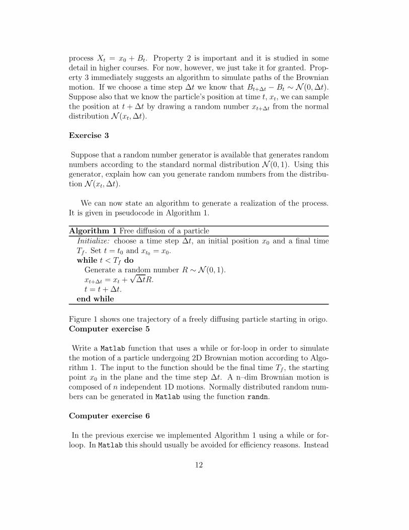
We can now state an algorithm to generate a realization of the process.It is given in pseudocode in Algorithm 1.

Algorithm 1 Free diffusion of a particle

Initialize: choose a time step ∆t, an initial position x0 and a final timeTf . Set t = t0 and xt0 = x0.while t < Tf do

Generate a random number R ∼ N (0, 1).xt+∆t = xt +

√∆tR.

t = t + ∆t.end while

Figure 1 shows one trajectory of a freely diffusing particle starting in origo.Computer exercise 5

Write a Matlab function that uses a while or for-loop in order to simulatethe motion of a particle undergoing 2D Brownian motion according to Algo-rithm 1. The input to the function should be the final time Tf , the startingpoint x0 in the plane and the time step ∆t. A n–dim Brownian motion iscomposed of n independent 1D motions. Normally distributed random num-bers can be generated in Matlab using the function randn.

Computer exercise 6

In the previous exercise we implemented Algorithm 1 using a while or for-loop. In Matlab this should usually be avoided for efficiency reasons. Instead

12

−0.2 0 0.2 0.4 0.6 0.8 1 1.2−0.8

−0.6

−0.4

−0.2

0

0.2

0.4

0.6

x

y

Figure 1: One path of a freely diffusing particle simulated with Algorithm 1.

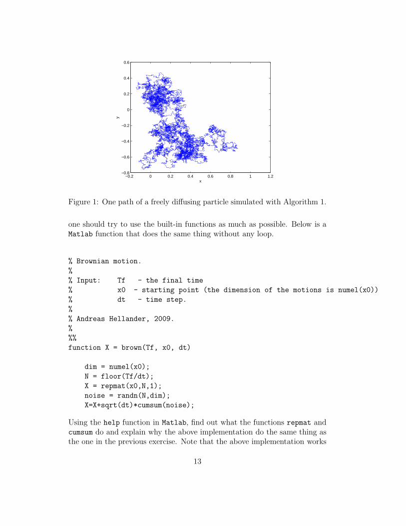
one should try to use the built-in functions as much as possible. Below is aMatlab function that does the same thing without any loop.

% Brownian motion.

%

% Input: Tf - the final time

% x0 - starting point (the dimension of the motions is numel(x0))

% dt - time step.

%

% Andreas Hellander, 2009.

%

%%

function X = brown(Tf, x0, dt)

dim = numel(x0);

N = floor(Tf/dt);

X = repmat(x0,N,1);

noise = randn(N,dim);

X=X+sqrt(dt)*cumsum(noise);

Using the help function in Matlab, find out what the functions repmat andcumsum do and explain why the above implementation do the same thing asthe one in the previous exercise. Note that the above implementation works

13

in arbitrarily dimensions.

Computer exercise 7

Implement the function in the previous exercise and, using the functions ticand toc, compare the time required to generate a realization with Tf = 1,x0 = [0, 0] and ∆t = 1e − 8 using the implementation with a loop and theone without. Which implementation requires most memory?

Computer exercise 8

There are several interesting questions one can ask about a particle un-dergoing Brownian motion. One such questions is, giving that the particlestarts its motion in the center of the interval (a, b), what is the average timeuntil the particle leaves that interval, E[τ ]. For a 1D Brownian motion, thisproblem has a simple analytical solution, E[τ ] = (b − a)2. We will now tryto verify this using a simulation.

a.)

Modify the codes from the previous exercises (which variant is most suitablein this case?) to simulate the Brownian motion until it exits the interval(a, b) and then, return the time that passed. The function should look like

function exit_time = brown_exit(interval, x0, dt)

where the first argument is the interval given as a vector [a, b] and x0 and dtis as in the previous exercises.

b.)

Using the function from a.), write a script that computes the mean value ofthe exit time based on M = 100 realizations. Let the particle start in origoand take the interval (−0.5, 0.5). Compare this value with the analyticalsolution.

c.)

Repeat the calculation in b.) for an increasing number of realizations, M =100, M = 1000, M = 10000. Compute the error in the solutions and comparethem for the different values of M . What appears to be the convergence rateas a function of M?

14

4.2 A biochemical control network

Recently, stochastic models of biochemical reaction networks have attractedmuch interest in the field of (computational) systems biology, a field con-cerned with understanding cellular processes on a systems level. A cell, thedomain where the reactions take place, is very small. In a popular modelorganism, the bacterium E. coli, the cellular volume is approximately 10−15l.Due to the small volume, some of the proteins involved in the reactions maybe present in only 1 − 10 copies. It has been illustrated in several papersthat the classical ODE models based on concentrations or mean values fail todescribe some properties of such systems as accurately as stochastic modelscan, and in this section we will study the model from one of those papers [6]in some detail. In particular, we will see how we can simulate biochemicalnetworks stochastically.

The mathematical model we will be using is a continuous time discretespace Markov Process (CTMC), and this is a very fundamental mathemati-cal formalism with applications in numerous fields of applied mathematics,physics, chemistry and computer science. Even though we will formulatethe algorithm to simulate such models in the context of biochemistry here,the same algorithm is a general method to simulate CTMCs, and thus hasapplications in other fields too, possibly under a different name.

The biochemical model we will study is a prototype model of a circadianrhythm. These kind of systems are responsible for adapting a cell or speciesto periodic oscillations in the environment, the most well known being thedaily rhythm of approximately 24h. This model includes two genes, theircorresponding mRNA and the proteins that are synthesized from the mRNA.However, before we can look at the properties of the model we need to developthe algorithm that we will rely on for simulations. We will also introducesome notation used when describing chemical reactions in a stochastic setting.

4.2.1 The stochastic simulation algorithm (SSA)

We write a chemical reaction between two chemical species A and B thatreact and form the species C as

A + Bω(a,b)−−−→ C. (12)

We assume mass action kinetics, and the propensity function ω(a, b) forthe reaction is a polynomial, ω(a, b) = kaab. This notation is common bothin the deterministic ODE formalism and in stochastic models, but the modelsdiffer in the interpretation of a and b and ω(a, b). The first difference is thatin the stochastic model a and b take values in the positive integers, Z+, and is

15

the number of molecules of the species, while in the deterministic model theyare the concentration and thus real valued. Secondly, in the deterministicmodel, the propensity function would be interpreted as the rate with whichthe reaction occurs, and using the rates for all the reactions in the modelwe formulate equations for the rate of change of each species; the ODEsystem. In the stochastic model on the other hand, the propensity functionis interpreted as the probability per unit time that the reaction occurs. Eachreaction is then treated as a discrete jump from one state to another, changingthe state by integer amounts. The reaction in (12) decreases A and B byone, and increases C by one.

Introducing the stoichiometry vector n = [−1,−1, 1] and the state vectorx = [a, b, c], we write a reaction r as

xωr(x)−−−→ x + nr. (13)

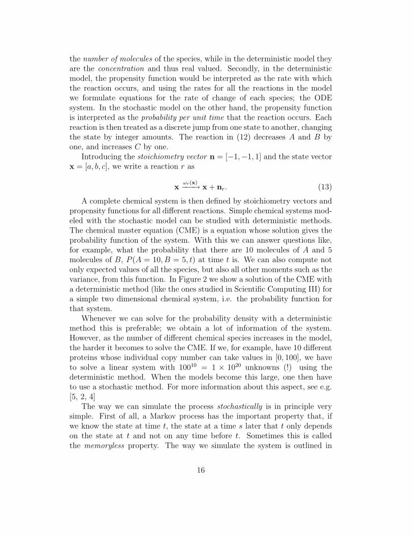
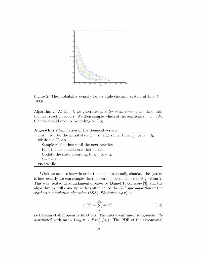
A complete chemical system is then defined by stoichiometry vectors andpropensity functions for all different reactions. Simple chemical systems mod-eled with the stochastic model can be studied with deterministic methods.The chemical master equation (CME) is a equation whose solution gives theprobability function of the system. With this we can answer questions like,for example, what the probability that there are 10 molecules of A and 5molecules of B, P (A = 10, B = 5, t) at time t is. We can also compute notonly expected values of all the species, but also all other moments such as thevariance, from this function. In Figure 2 we show a solution of the CME witha deterministic method (like the ones studied in Scientific Computing III) fora simple two dimensional chemical system, i.e. the probability function forthat system.

Whenever we can solve for the probability density with a deterministicmethod this is preferable; we obtain a lot of information of the system.However, as the number of different chemical species increases in the model,the harder it becomes to solve the CME. If we, for example, have 10 differentproteins whose individual copy number can take values in [0, 100], we haveto solve a linear system with 10010 = 1 × 1020 unknowns (!) using thedeterministic method. When the models become this large, one then haveto use a stochastic method. For more information about this aspect, see e.g.[5, 2, 4]

The way we can simulate the process stochastically is in principle verysimple. First of all, a Markov process has the important property that, ifwe know the state at time t, the state at a time s later that t only dependson the state at t and not on any time before t. Sometimes this is calledthe memoryless property. The way we simulate the system is outlined in

16

A

B

0 10 20 30 40 50 60 70 80 90 1000

10

20

30

40

50

60

70

80

90

100

Figure 2: The probability density for a simple chemical system at time t =1000s.

Algorithm 2. At time t, we generate the inter event time τ , the time untilthe next reaction occurs. We then sample which of the reactions r = 1 . . .Nr

that we should execute according to (13).

Algorithm 2 Simulation of the chemical system.

Initialize: Set the initial state x = x0 and a final time Tf . Set t = t0.while t < Tf do

Sample τ , the time until the next reaction.Find the next reaction r that occurs.Update the state according to x = x + nr.t = t + τ .

end while

What we need to know in order to be able to actually simulate the systemis how exactly we can sample the random numbers τ and r in Algorithm 2.This was treated in a fundamental paper by Daniel T. Gillespie [3], and thealgorithm we will come up with is often called the Gillespie algorithm or thestochastic simulation algorithm (SSA). We define a0(x) as

a0(x) =Nr∑

r

ωr(x), (14)

i.e the sum of all propensity functions. The inter event time τ is exponentiallydistributed with mean 1/a0, τ ∼ Exp(1/a0). The PDF of the exponential

17

distribution is given in (15).

f(τ ; a0) =

a0e−a0τ , τ ≥ 0

0, τ < 0.(15)

In the next exercise we will show how we can generate a random number τfrom this distribution if we have access to random numbers from the uniformdistribution U(0, 1). This will tell us how to actually do step one in Algo-rithm 2. The method we will use is inverse transform sampling and is givenin Algorithm 3.

Algorithm 3 Inverse transform sampling.

Generate a random number u from U(0, 1).Compute τ such that F (τ) = u.Take τ as a random number from the distribution defined by F .

F (τ) is the cumulative distribution function (CDF) and in the next exercisewe will apply this procedure to generate random numbers from the exponen-tial distribution.

Exercise 4

a.)

The CDF is defined as

F (t) = P (τ ≤ t) =

∫ t

−∞

f(τ ; a0)dτ,

where F (τ ≤ t) is the probability that τ is smaller that or equal to t. Forthe exponential distribution as defined in (15), compute the CDF.

b.)

Find the inverse of F (τ), i.e. for a number u find τ such that F (τ) = u, orin other words τ = F−1(u). Remark: This procedure is general, but for manydistributions there is no simple, closed form for the inverse CDF and themethod may be computational expensive. For some important distributionsthere are other, more efficient methods available to generate random numbers.

We are now ready to update Algorithm 2.The only remaining issue before we have a complete algorithm to simulatethe biochemical system is a method to generate the next reaction that occurs.The next reaction is a random variable Y with distribution [3]

18

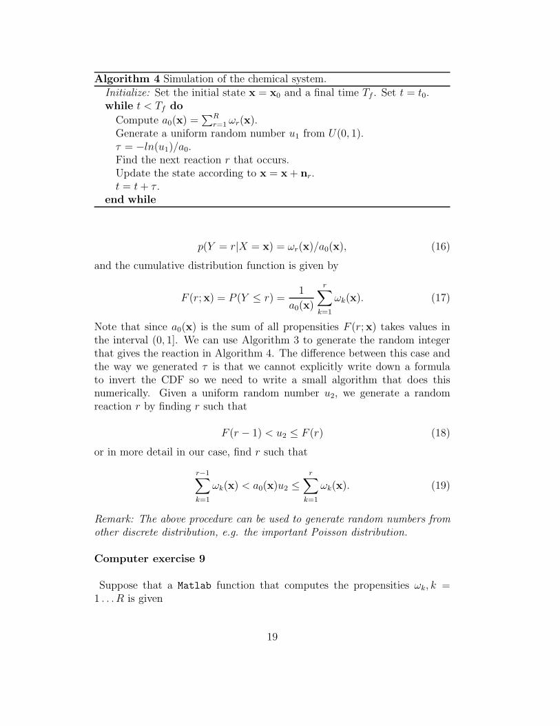
Algorithm 4 Simulation of the chemical system.

Initialize: Set the initial state x = x0 and a final time Tf . Set t = t0.while t < Tf do

Compute a0(x) =∑R

r=1 ωr(x).Generate a uniform random number u1 from U(0, 1).τ = −ln(u1)/a0.Find the next reaction r that occurs.Update the state according to x = x + nr.t = t + τ .

end while

p(Y = r|X = x) = ωr(x)/a0(x), (16)

and the cumulative distribution function is given by

F (r;x) = P (Y ≤ r) =1

a0(x)

r∑

k=1

ωk(x). (17)

Note that since a0(x) is the sum of all propensities F (r;x) takes values inthe interval (0, 1]. We can use Algorithm 3 to generate the random integerthat gives the reaction in Algorithm 4. The difference between this case andthe way we generated τ is that we cannot explicitly write down a formulato invert the CDF so we need to write a small algorithm that does thisnumerically. Given a uniform random number u2, we generate a randomreaction r by finding r such that

F (r − 1) < u2 ≤ F (r) (18)

or in more detail in our case, find r such that

r−1∑

k=1

ωk(x) < a0(x)u2 ≤r

∑

k=1

ωk(x). (19)

Remark: The above procedure can be used to generate random numbers fromother discrete distribution, e.g. the important Poisson distribution.

Computer exercise 9

Suppose that a Matlab function that computes the propensities ωk, k =1 . . . R is given

19

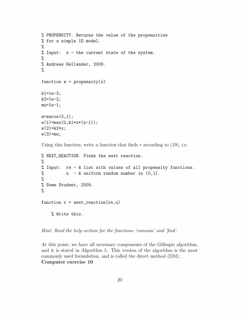
% PROPENSITY. Returns the value of the propensities

% for a simple 1D model.

%

% Input: x - the current state of the system.

%

% Andreas Hellander, 2009.

%

function w = propensity(x)

k1=1e-3;

k2=1e-2;

mu=1e-1;

w=zeros(3,1);

w(1)=max(0,k1*x*(x-1));

w(2)=k2*x;

w(3)=mu;

Using this function, write a function that finds r according to (19), i.e.

% NEXT_REACTION. Finds the next reaction.

%

% Input: re - A list with values of all propensity functions.

% u - A uniform random number in (0,1].

%

% Some Student, 2009.

%

function r = next_reaction(re,u)

% Write this.

Hint: Read the help section for the functions ’cumsum’ and ’find’.

At this point, we have all necessary components of the Gillespie algorithm,and it is stated in Algorithm 5. This version of the algorithm is the mostcommonly used formulation, and is called the direct method (DM).Computer exercise 10

20

Algorithm 5 Gillespie’s direct method (DM)

Initialize: Set the initial state x = x0 and a final time Tf . Set t = t0.while t < Tf do

Compute a0(x) =∑R

r=1 ωr(x).Generate two uniform random number u1, u2 from U(0, 1).τ = −ln(u1)/a0.Find r such that

∑r−1k=1 ωk(x) < a0(x)u2 ≤

∑rk=1 ωk(x).

Update the state according to x = x + nr.t = t + τ .

end while

Implement Algorithm 5 and apply it on the propensities given by the func-tion propensity in the previous exercise. The stoichiometry vectors aren1 = −2, n2 = −1, n2 = 1. The input to the function should be a functionthat computes the propensities, a function that gives the stoichiometry ma-trix, the initial state and a vector that specifies the output times.

4.2.2 The circadian rhythm

Now that we have formulated and tested Gillespie’s direct method on a simplemodel problem in Computer exercise 10 we will use it to study the moreinvolved model in [6]. For the particular system we are considering herethere are 18 reactions and they are found in (20).

D′

a

θaD′

a−−−→ Da

Da + AγaDaA−−−−→ D′

a

D′

r

θrD′

r−−−→ Dr

Dr + AγrDrA−−−−→ D′

r

∅ α′

aD′

a−−−→ Ma

∅ αaDa−−−→ Ma

MaδmaMa−−−−→ ∅

∅ βaMa−−−→ A

∅ θaD′

a−−−→ A

∅ θrD′

r−−−→ A

AδaA−−→ ∅

A + RγcAR−−−→ C

∅ α′

rD′

r−−−→ Mr

∅ αrDr−−−→ Mr

MrδmrMr−−−−→ ∅

∅ βrMr−−−→ R

RδrR−−→ ∅

CδaC−−→ R

(20)

The parameters of the model are given in Table 1. The complete propensityfunctions ωr, r = 1 . . . 18 are given above the arrows.

21

αA α′

a αr α′

r βa βr δma δmr

50.0 500.0 0.01 50 50.0 5.0 10.0 0.5δa δr γa γr γc Θa Θr

1.0 0.2 1.0 1.0 2.0 50.0 100.0

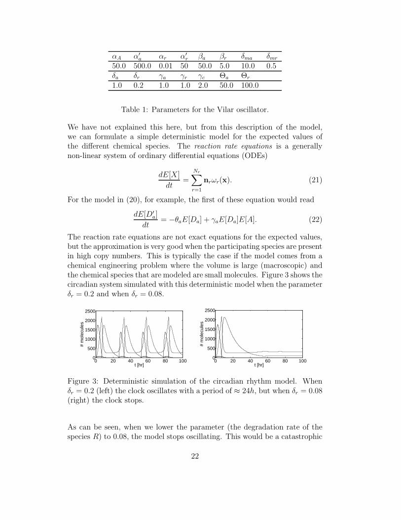
Table 1: Parameters for the Vilar oscillator.

We have not explained this here, but from this description of the model,we can formulate a simple deterministic model for the expected values ofthe different chemical species. The reaction rate equations is a generallynon-linear system of ordinary differential equations (ODEs)

dE[X]

dt=

Nr∑

r=1

nrωr(x). (21)

For the model in (20), for example, the first of these equation would read

dE[D′

a]

dt= −θaE[Da] + γaE[Da]E[A]. (22)

The reaction rate equations are not exact equations for the expected values,but the approximation is very good when the participating species are presentin high copy numbers. This is typically the case if the model comes from achemical engineering problem where the volume is large (macroscopic) andthe chemical species that are modeled are small molecules. Figure 3 shows thecircadian system simulated with this deterministic model when the parameterδr = 0.2 and when δr = 0.08.

0 20 40 60 80 1000

500

1000

1500

2000

2500

t [hr]

# m

olec

ules

0 20 40 60 80 1000

500

1000

1500

2000

2500

t [hr]

# m

olec

ules

Figure 3: Deterministic simulation of the circadian rhythm model. Whenδr = 0.2 (left) the clock oscillates with a period of ≈ 24h, but when δr = 0.08(right) the clock stops.

As can be seen, when we lower the parameter (the degradation rate of thespecies R) to 0.08, the model stops oscillating. This would be a catastrophic

22

event for a living cell, and one would expect that the presence of oscillationswould be more robust to changes in the parameters. Using this ODE model,however, we will inevitably get this sharp switch like behavior. In the paper[6], one also considers the stochastic model discussed in the previous section.We will now try to reproduce the conclusion from that paper.

Computer exercise 11

Simulate a single trajectory of the model defined by (20) and Table 1 usingthe algorithm you implemented in Computer exercise 10. Plot trajectoriescorresponding to δr = 0.2, δr = 0.08 and δr = 0.01. Does the stochasticmodel display the same sharp ”on–off” behavior as the deterministic ODEmodel does? Compare your simulations to the conclusions in paper [6].

5 Summary

In these lecture notes, we have seen examples where stochastic simulationand Monte Carlo methods were used to study different processes. We havealso seen how to use pseudo random numbers to evaluate integrals. MonteCarlo becomes an alternative to deterministic methods for solving scientificproblems in a number of different scenarios, but are often considered as amethod of last resort; they are used when no deterministic methods is avail-able or computationally feasible. The reason for this is the slow convergenceof Monte Carlo methods (O(N−1/2)), making them very computationallydemanding if result with a high accuracy is desired.

For the integration example, it is not in principle hard to formulate deter-ministic quadrature rules to solve high dimensional integrals, but the numberof quadrature points grows exponentially with the dimension. Their conver-gence rate is also sensitive to both the dimensionality and the smoothness ofthe integrand. When there is no longer possible to use these methods, MonteCarlo can still compute a result. However, no one would use Monte Carlointegration to compute an approximation to an integral in say two or threedimensions; deterministic methods are much more efficient in this case.

In another example of a biochemical control network we have seen thata simple stochastic model gives a better description of the system than thesimple deterministic model. Even if we could formulate a complicated de-terministic model that describe the system as good as the stochastic model,we rather use a simple stochastic model. Also in this case, depending on thequestion we are asking, we are presented with a choice between using a de-

23

terministic or stochastic method to study the stochastic model. Also in thiscase, if the deterministic method is applicable, we would use it. However, thecomputational work for the deterministic method grows exponentially withthe number of different chemical species in the model, so for models withmany species we have to resort to a stochastic simulation method, SSA.

Obviously, there are numerous of application areas in scientific comput-ing where Monte Carlo can be used that we have not mentioned here, e.g.optimization, stochastic differential equations and solution of partial differ-ential equations to name a few. However, it is the hope that you at this pointunderstand the basic ideas behind Monte Carlo methods. The same ideasand workflow as we have seen here applies to many other situations, eventhough the details may be different.

References

[1] Steven C. Chapra. Applied Numerical Methods with MATLAB for Engi-neers and Scientists. McGraw–Hill, second edition, intenational edition,2008.

[2] Stefan Engblom. Numerical Solution Methods in Stochastic ChemicalKinetics. PhD thesis, Uppsala University, 2008.

[3] Daniel T Gillespie. A general method for numerically simulating thestochastic time evolution of coupled chemical reacting systems. J. Com-put. Phys., 22:403–434, 1976.

[4] Andreas Hellander. Numerical simulation of well stirred biochemical re-action networks governed by the master equation. Licentiate thesis, De-partment of Information Technology, Uppsala University, 2008.

[5] Paul Sjoberg. Numerical Methods for Stochastic Modeling of Genes andProteins. PhD thesis, Uppsala University, 2007.

[6] Jose M. G. Vilar, Hau Yuan Kueh, Naama Barkai, and Stanislav Leibler.Mechanisms of noise resistance in genetic oscillators. Proc. Nat. Acad.Sci. USA, 99(9):5988–5992, 2002.

24