stochastic source modelling and tsunami analysis of the
TRANSCRIPT

Western University Western University
Scholarship@Western Scholarship@Western
Electronic Thesis and Dissertation Repository
8-24-2021 9:30 AM
Stochastic Source Modelling and Tsunami Analysis of the 2012 Stochastic Source Modelling and Tsunami Analysis of the 2012
Mw 7.8 Haida Gwaii Earthquake Mw 7.8 Haida Gwaii Earthquake
Karina Martinez Alcala, The University of Western Ontario
Supervisor: Goda, Katsuichiro, The University of Western Ontario
Joint Supervisor: Mora-Stock,Cindy, The University of Western Ontario
A thesis submitted in partial fulfillment of the requirements for the Master of Science degree in
Geophysics
© Karina Martinez Alcala 2021
Follow this and additional works at: https://ir.lib.uwo.ca/etd
Part of the Geophysics and Seismology Commons, and the Other Earth Sciences Commons
Recommended Citation Recommended Citation Martinez Alcala, Karina, "Stochastic Source Modelling and Tsunami Analysis of the 2012 Mw 7.8 Haida Gwaii Earthquake" (2021). Electronic Thesis and Dissertation Repository. 8145. https://ir.lib.uwo.ca/etd/8145
This Dissertation/Thesis is brought to you for free and open access by Scholarship@Western. It has been accepted for inclusion in Electronic Thesis and Dissertation Repository by an authorized administrator of Scholarship@Western. For more information, please contact [email protected].

ii
Abstract
The Mw 7.8 2012 Haida Gwaii Earthquake triggered a tsunami that highlighted the
importance of tsunami hazard assessment on Canada’s Pacific coast. Stochastic source
modelling serves as a valuable method to assess future tsunami hazard and has not been
performed for this region. The source models characterize the uncertainty of earthquake
ruptures by considering variability in fault geometry and slip heterogeneity, which, in turn,
allows the consideration of a wide range of tsunami scenarios in the Haida Gwaii region.
The model predictions are constrained by observational data and past source inversion
studies. One hundred twenty-eight stochastic tsunami scenarios are generated using the
stochastic source modelling method to assess tsunami hazard via tsunami inundation
simulations of the target region and conduct sensitivity analyses of tsunami height
variability. The resulting models can promote better-informed risk management decisions
and future probabilistic tsunami hazard analysis in this region.
Keywords
Stochastic source modelling, stochastic models, tsunami hazard, Monte Carlo tsunami
simulation, 2012 Haida Gwaii earthquake, tsunamis, slip distributions

iii
Summary for Lay Audience
On October 28, 2012, an Mw 7.8 earthquake hit the region of Haida Gwaii, Canada. The
tsunami triggered by the earthquake was recorded across the Pacific Ocean. Horizontal and
vertical deformations were obtained months after the earthquake and, during post event
field surveys, run-up levels were measured at several locations within the rupture zone.
This study conducts a tsunami analysis of the Haida Gwaii region using stochastic source
modelling and performs Monte Carlo tsunami simulation to develop source models that
generate tsunami waves in close match with the recorded observations. The developed
stochastic earthquake source model can be applied to evaluate tsunami hazards due to future
tsunamigenic events in Haida Gwaii. The methodology encompasses the wavenumber
analysis of six existing earthquake slip models to define a generic fault model for the
synthetic slip source generation. The stochastic source parameters are based on earthquake
source scaling relations derived from global models. The stochastic method uses spectral
synthesis, where key slip characteristics are specified in slip statistics, slip distribution
parameters, and asperity areas. For a given set of stochastic synthesis parameters, slip
distributions are generated by a Fourier integral method. The derived stochastic models can
capture realistic asperity zones and source parameters close to those of the 2012 event.
Asperity zones are mainly located on the shallow ocean side of the fault, which is consistent
with the epicentre location constrained by seismic and deformation data. Consequently,
simulated tsunami waves at different stations show that first wave amplitudes are in
agreement with the observations. Simulated tsunami run-ups are generally consistent with
those observed at sites sheltered from storm waves, with differences ranging from 0.5−3
m. In contrast, the differences become significant at sites exposed to storm waves with a
discrepancy of up to 7 m. The discrepancy may be attributed to the possibility that run-up
survey observations at exposed bays might include effects due to major storm events that
hit Haida Gwaii between the earthquake and the survey. Moreover, source parameters and
models that are calibrated for the 2012 event can be adopted to evaluate tsunamis due to
future large events in the region.

iv
Co-Authorship Statement
The present thesis, along with the MATLAB codes used in the research were done in co-
authorship with Dr. Katsuichiro Goda. Dr. Goda provided feedback on all thesis chapters
as well as provided the base MATLAB codes used for the synthesis of stochastic models
and tsunami simulations.

v
Acknowledgments
I want to express my deep gratitude to my supervisor Dr. Katsuichiro Goda for his support
and guidance, as well as, the time and effort he put into helping me develop the computer
codes needed for the research and revising my thesis. This project could not have been
accomplished without his help and dedication. It has been a true honour to be your student.
To my co-supervisor, Cindy Mora-Stock, and the research group, Yusong Yang and Elisa
Dong, who listened to my presentations and gave me ideas for improvement, thank you for
your extensive help. A special gratitude goes to Payam Momeni; without your countless
guidance, patience, and encouragement, this thesis would not have been completed. I am
forever grateful to your help.
I also want to thank the three members of my thesis committee, Dr. Schincariol, Dr.
Assatourians, and Dr. McBean, for taking the time to read my thesis and provide useful
comments for improvement.
I want to extend my thanks to SHARCNET and Ocean Networks Canada for their
continued support to Dr. Goda and the rest of the research group.
To my friends Rhys Paterson, Melissa Contreras, Gerardo Garay, and Pedro Ibarra thank
you for being by my side and always believing in me even when I didn't. You have been a
genuine emotional support throughout this journey.
Finally, to my family and partner. There are no words to express how grateful and in debt
I am with you. Mom and Dad, thank you for all your sacrifices that have allowed me always
to reach my dreams. This accomplishment is yours. Cruz Estrella, thank you for always
being there for me, the countless words of encouragement, the immense support, and for
constantly pushing me to be better; without you, I couldn't have started this Master’s.

vi
Table of Contents
Abstract ............................................................................................................................... ii
Summary for Lay Audience ............................................................................................... iii
Co-Authorship Statement ................................................................................................... iv
Acknowledgments ............................................................................................................... v
Table of Contents ............................................................................................................... vi
List of Tables ..................................................................................................................... ix
List of Figures ..................................................................................................................... x
Chapter 1 ............................................................................................................................. 1
1 Introduction .................................................................................................................... 1
1.1 Objectives ............................................................................................................... 6
1.2 Thesis Structure ...................................................................................................... 6
Chapter 2 ............................................................................................................................. 8
2 Overview of Principal Concepts and Techniques for Stochastic Source Modelling
and Tsunami Simulation ................................................................................................ 8
2.1 Earthquake Source Modelling ............................................................................... 10
2.2 Stochastic Source Models ..................................................................................... 12
2.3 Tsunami Simulations ............................................................................................ 14
Chapter 3 ........................................................................................................................... 24
3 Stochastic Source Modelling and Tsunami Analysis of the 2012 Mw 7.8 Haida
Gwaii Earthquake ......................................................................................................... 24
3.1 2012 Haida Gwaii Event ....................................................................................... 25
3.2 Tectonics and Seismicity of the Haida Gwaii Region .......................................... 27
Margin Convergence and Underthrusting ................................................. 27
Fault Geometry ......................................................................................... 28
3.3 Observations ......................................................................................................... 29

vii
Deformation .............................................................................................. 31
Tide Gauges .............................................................................................. 33
Deep-Ocean Observations ........................................................................ 35
Run-up Observations ................................................................................ 36
3.4 Inversion Models .................................................................................................. 38
3.5 Earthquake Scenario ............................................................................................. 41
3.6 Source Parameters ................................................................................................. 46
3.7 Stochastic Sources ................................................................................................ 47
3.8 Monte Carlo Tsunami Simulations ....................................................................... 49
Bathymetry ................................................................................................ 49
Nested Grid Formulations ......................................................................... 50
Tsunami Inundation Simulation ................................................................ 53
3.9 Results ................................................................................................................... 54
Literature Finite-Fault Models .................................................................. 54
Simulated Stochastic Source Models ........................................................ 57
Offshore Tsunami Result: Comparison with Observations ...................... 61
Onshore Tsunami Results: Comparison with Run-up Observations ........ 71
3.10 Conclusions ........................................................................................................... 73
Chapter 4 ........................................................................................................................... 74
4 Future Tsunami Scenarios for the Haida Gwaii Region .............................................. 74
4.1 Procedure .............................................................................................................. 76
4.2 Results ................................................................................................................... 79
Simulated Stochastic Source Models ........................................................ 79
Far-Field Results ....................................................................................... 82
Near field Results ...................................................................................... 85

viii
4.3 Conclusions ........................................................................................................... 87
Chapter 5 ........................................................................................................................... 88
5 Conclusions .................................................................................................................. 88
5.1 Limitations ............................................................................................................ 89
5.2 Future Work .......................................................................................................... 90
References ......................................................................................................................... 91
Appendix A ..................................................................................................................... 104
Appendix B ..................................................................................................................... 114
Curriculum Vitae ............................................................................................................ 116

ix
List of Tables
Table 3.1 Coseismic offsets at GPS stations in the Haida Gwaii region ........................... 31
Table 3.2 Wave parameters of the October 28, 2012 Haida Gwaii tsunami derived from
tide gauge observations on the northwestern Pacific ......................................................... 34
Table 3.3 Wave parameters of the October 28, 2012 Haida Gwaii tsunami derived from
deep-sea observations on the northwestern Pacific............................................................ 36
Table 3.4 Tsunami runup and inundation data of the 2012 Haida Gwaii tsunami ............ 37
Table 3.5 Parameters of inversion models from literature ................................................. 38
Table 3.6 Summary of the finite fault source parameters for the 2012 Haida Gwaii
earthquake .......................................................................................................................... 42
Table 3.7 Linear correlation coefficients of regression residuals of the scaling
relationships for the earthquake source parameters ........................................................... 47
Table 3.8 Summary of stochastic earthquake slip simulation parameters ......................... 57
Table 3.9 Sum of square errors of the tsunami observations and deformation for the six
literature models and best stochastic source models .......................................................... 63
Table 3.10 Run-up values for nine stochastic sources along the Haida Gwaii region ....... 72
Table 4.1 Summary of stochastic earthquake slip simulation parameters ......................... 78

x
List of Figures
Figure 1.1 Haida Gwaii region on the Pacific Ocean northwest, showing epicentre of the
largest earthquakes in the zone (red and orange stars). The locations of the longest ground
motions are also shown (pink rectangle). ............................................................................ 3
Figure 2.1 Geometry of the source model. From Physics of Tsunamis (p. 46) by Levin, B.
& Nosov, M., 2009, Springer. Copyright 2009 by Springer Science + Business Media
B.V(2.1) ............................................................................................................................. 16
Figure 2.2 Formulation of the problem of a tsunami run-up on the coast (Levin & Nosov,
2009) .................................................................................................................................. 22
Figure 3.1 a) location of the thrust fault beneath the QCT in which the 2012 earthquake
occurred, the relative plate motions in this area, and location of the near-vertical QFC
(Cassidy et al., 2014). (b) Surface temperatures, two possible geometries of ................... 25
Figure 3.2 Map of Haida Gwaii showing the locations of FOC and NOAA tide gauges,
Ocean Network Canada BPRs and DART buoys that recorded the 2012 Haida Gwaii
tsunami ............................................................................................................................... 30
Figure 3.3 a) Horizontal deformation by GPS measurements. b) vertical deformation by
intertidal biological indicators and GPS measurements .................................................... 32
Figure 3.4 Time histories of the 2012 Haida Gwaii tsunami waves at FOC and NOAA
tide gauges ......................................................................................................................... 33
Figure 3.5 Time histories of the 2012 Haida Gwaii tsunami waves at ONC's BPRs and
DART buoys ...................................................................................................................... 35
Figure 3.6 Run-up sites with colors depending on amount of run-up ............................... 37
Figure 3.7 Figure 3.8 Finite fault models a) Lay et al., (2013). b) Wei (2012). c) Shao & Ji
(2012). d) Hayes (2013) (Fine et al., 2015). e) Gusman et al., (2016). f) Hayes (2017) ... 40
Figure 3.8 Tsunami source zone model for the Haida Gwaii region ................................. 44

xi
Figure 3.9 Map showing the synthetic fault plane (black) and the asperity zone (red) ..... 45
Figure 3.10 Flow chart of the stochastic method ............................................................... 48
Figure 3.11 Tsunami computational domains (810 m-270 m-90 m-30 m) ........................ 52
Figure 3.12 Tsunami waveforms at Queen Charlotte, Henslung Cove, Crescent City,
Cascadia Basin, Barkley Canyon and DART 46410 stations and literature models ......... 55
Figure 3.13 Horizontal and Vertical deformation vectors of the observations and source
models from the literature .................................................................................................. 56
Figure 3.14 (a-e) Five stochastic models (Mw 7.7-7.9), and (f) overall average slip
models based on the 1000 stochastic sources .................................................................... 58
Figure 3.15 Horizontal and vertical deformations of observations and stochastic models 59
Figure 3.16 Comparison of estimated source parameters for the stochastic models and six
models from literature against the corresponding global scaling relationships ................. 60
Figure 3.17 Comparison of time histories of tsunami wave for the 128 and 168 stochastic
models (mean, 90th percentile, and 90th percentile) and the Gusman et al. (2016) model
with the observations at different tide gauges .................................................................... 64
Figure 3.18 Comparison of time histories of tsunami wave for the 128 and 168 stochastic
models (mean, 90th percentile, and 90th percentile) and the Gusman et al. (2016) model
with the observations at different ONC BPRs and DART buoys ...................................... 65
Figure 3.19 Figure 3.20 Stochastic source models for the 2012 Haida Gwaii earthquake
with slip distributions ......................................................................................................... 66
Figure 3.20 Sites near the coast of Haida Gwaii ................................................................ 66
Figure 3.21 Time histories of tsunami waves for sites 5, 7,12, and 14 .............................. 67
Figure 3.22 Time histories of tsunami waves for locations 15,16, 18, and 20 .................. 68
xii
Figure 3.23 a) Maximum coastal tsunami wave heights generated by the eight stochastic
models and the Gusman et al. (2016) model, and b) sites along the shoreline of Haida
Gwaii .................................................................................................................................. 69
Figure 3.24 Maximum wave height for the Haida Gwaii region ....................................... 70
Figure 4.1 The Oshawa rise, Queen Charlotte Trough (trench), Queen Charlotte terrace
(accretionary sedimentary prism), and Queen Charlotte ranges (uplifted edge of
continent). The dashed lines show the model extent of the underthrust plate for 2.5 and 6
million years, that is, for the triple junction at Brooks Peninsula (from 6 Ma) and at the
Wilson Knolls (from 2.5 Ma). It is assumed that there has been no significant crustal
shortening in these estimates. (Hyndman, 2015) ............................................................... 75
Figure 4.2 Map showing the synthetic fault plane (black) and the asperity zone (red)
defined for this study ......................................................................................................... 76
Figure 4.3 Comparison of 326 stochastic source parameters (green dots) with the
corresponding scaling relationships. .................................................................................. 80
Figure 4.4 (a-e) Five stochastic models (Mw 7.9-8.1), and (f) overall average slip models
based on the 326 stochastic sources ................................................................................... 81
Figure 4.5 Comparison of time histories of tsunami wave for the 326 stochastic models
(mean, 90th, and 10th percentile) and observations........................................................... 83
Figure 4.6 Comparison of time histories of tsunami wave for the 326 stochastic models
(mean, 90th, and 10th percentile) and observations........................................................... 84
Figure 4.7 Maximum wave height for the Haida Gwaii region ......................................... 86

xiii
List of Appendices
Appendix A:1 Time histories of the six literature models against observations ............. 104
Appendix A:2 Time histories of the six literature models against observations ............. 105
Appendix A: 3 Horizontal and Vertical deformation vectors of the observations and
source models from the literatures ................................................................................... 106
Appendix A: 4 Horizontal and Vertical deformation vectors of the observations and
source models from the literatures ................................................................................... 107
Appendix A: 5 Horizontal and vertical deformations of observations and stochastic
models .............................................................................................................................. 108
Appendix A: 6 Tsunami waveforms at Tofino, Ketchikan, DART 46404, DART 46407
stations and literature models ........................................................................................... 108
Appendix A: 7 Horizontal and vertical deformations of observations and stochastic
models .............................................................................................................................. 109
Appendix A:8 Time histories of tsunami waves for sites 1, 2, 3, 4, 6, 8 ......................... 110
Appendix A:9 Time histories of tsunami waves for sites 9, 10, 11, 13 ........................... 111
Appendix A:10 Time histories of tsunami waves for sites 17-19 .................................... 111
Appendix A:11 Maximum wave height for the Haida ..................................................... 112
Appendix A:12 Run-up values for six literature sources along the Haida Gwaii region. 113
Appendix B:1: Comparison of time histories of tsunami wave for the 326 stochastic
models (mean, 90th and 10th percentile) and observations ............................................... 114
Appendix B:2: Maximum wave height for the Haida Gwaii region ................................ 115

1
Chapter 1
1 Introduction
Tsunamis, a combination of two Japanese words translated in English as ‘wave in harbour,’
are a series of water waves caused by seismic activities, landslides, and volcanic eruptions.
Earthquakes are the principal source of tsunamis and cause the largest wave amplitudes
(Leonard et al., 2014). During an earthquake rupture, tsunamis are generated by
transforming large-scale elastic deformation to potential energy within the water column
(Levin & Nosov, 2009). The initial dislocation of a large volume of water then propagates
spatially due to gravity. During this process, a large amount of water is displaced and
eventually causes substantial flooding along coastlines. Thus, making tsunamis one of the
most destructive and deathly phenomena (Bernard & Titov, 2015). Coastal flooding is
caused by a shoaling process in which, as the tsunami approaches the coast, the wave
propagation speed decreases while the tsunami height increases. The increase in the
tsunami’s height is because the wave’s amplitude is a function of the propagation velocity,
which depends on depth. On the other hand, the tsunami wave loses its energy due to bottom
friction and turbulence.
Historical records show that tsunamis have had a significant socio-economic impact on
human history, as evidenced major destruction of coastal communities. Recent significant
tsunami events have also reminded us of the importance of tsunami hazard assessment,
particularly in highly populated coastal areas. For example, the 2004 Indian Ocean mega-
thrust earthquake of moment magnitude (Mw) 9.3 triggered a massive tsunami that reached
a maximum run-up of 30 m (Titov et al., 2005; Wang & Liu, 2006). This tsunami left
hundreds of thousands of deaths and billions of dollars in damages across 19 countries. The
lack of proper risk management decisions and early-warning system made the 2004 Indian
Ocean earthquake and tsunami one of the most devastating natural disasters in human
history (Ghobarah et al., 2006). This catastrophe prompted scientists and engineers to
design better early warning systems and develop new tsunami analysis techniques. The
most recent major event, the 2011 Tohoku earthquake and tsunami in Japan, left more than
19,000 fatalities and hundreds of billions of dollars in damages (Takabatake et al., 2019).

2
This event highlighted another issue in tsunami hazard assessment, the difficulty of
assessing the characteristics of future events. The Tohoku event was extreme because the
actual event was greater than what scientists and engineers previously thought this
subduction zone could generate. Therefore, the tsunami scenarios considered when
preparing the 2005 Japanese tsunami hazard maps were smaller, significantly
underestimating the tsunami hazard. An example was Iwate Prefecture of Japan, where
more than 65% of the casualties were outside the major inundation zones (Goda & Song,
2016). The uncertainty of future events affects risk management decisions, which could
ultimately fail to prevent major devastation and significant human casualties.
The western coast of North America is at risk of potential earthquakes and tsunamis. The
tsunami hazard is significantly higher in the Cascadia and Haida Gwaii region (Figure 1.1).
In the north, the Haida Gwaii region is located on a plate boundary between the North
American and Pacific Plates known as the Queen Charlotte Fault (QCF). The QCF is
characterized by its primary right-lateral shear in its northernmost part (Brothers et al.,
2020). The largest instrumentally recorded earthquake in Canada occurred in this region
(i.e. 1949 Mw 8.1 Queen Charlotte earthquake; Figure 1.1), and several other major
earthquakes of Mw>7 struck the region (i.e. 1899 Mw 8 Yakutat earthquake, 1958 Mw 7.7
Lituya earthquake, 1972 Mw 7.5 Sitka earthquake, 2013 Mw 7.5 Craig earthquake; Szeliga,
2013; Cassidy et al., 2014). The southern part of the QCF is characterized by a convergent
component which resulted in the 2012 Haida Gwaii earthquake. Several tectonic models
have been suggested for the evolution and mechanics of this part of the QCF. Hyndman
(2015) suggested that the convergence is accommodated by a subduction of the Pacific
Plate under the North American Plate. In contrast, other models suggest a partitioning of
the slip-motion on the QCF and convergent deformation on thrust and reverse faults in
Queen Charlotte Terrace (QCT; Tréhu et al., 2015, Brothers et al., 2020).In short, Haida
Gwaii is the most seismically active zone on the western coast.
South of the triple junction among the North American, Pacific, and Juan de Fuca Plate,
the Cascadia Subduction Zone (CSZ) exists. The CSZ results from the convergence of the
North American Plate onto the Juan de Fuca Plate and extends 1100 km along the coastal
margin from Vancouver Island, Canada, to the Mendocino Escarpment, northern

3
California, United States. The CSZ poses a triple seismic threat. Firstly, the subduction
earthquakes from the Juan de Fuca-North American convergence. Secondly, from the faults
in the overriding North American Plate. Lastly, from the intersection of the subduction zone
with the Mendocino transform fault on the San Andreas Fault in the south and the QCF in
the north (Petersen, 2002; Atwater et al., 2015). The CSZ is known to rupture in great Mw
8-9 thrust earthquakes with a recurrence period between 100 to 800 years (Goldfinger,
2012), the last one being the 1700 Mw 9 event. Thus, the subduction zone has the potential
to rupture in a mega-thrust subduction earthquake with an imminent threat of a tsunami,
which would cause extensive damage to highly populated zones along the Pacific coast.
Figure 1.1 Haida Gwaii region on the Pacific Ocean northwest, showing epicentre of the largest
earthquakes in the zone (red and orange stars). The locations of the longest ground motions are
also shown (pink rectangle).

4
Although Haida Gwaii is not a highly populated area, earthquakes and tsunamis produced
in the region can provide a valuable case study. It can help scientists and engineers better
understand the hazard and potential risks of similar or much larger earthquakes and
tsunamis in the CSZ (Leonard & Bednarski, 2014). Therefore, the geophysical and
geological information from the QCF past events can help validate forecasting models for
CSZ future events since the zone lacks information on past earthquakes (Leonard et al.,
2014). Tsunami hazard assessment in the Pacific’s northwest is critical because of the
development that has taken place in coastal communities. This development makes the
social and economic impact of future tsunami events more severe than in the past.
Therefore, it is crucial to plan and assess for future scenarios. Furthermore, such
assessments will inform communities of inundation zones and possible hazards (Bernard
& Titov, 2015). Consequently, making the Haida Gwaii region an interesting and important
zone for research.
Tsunami inversion and simulation studies are essential for enhancing tsunami preparedness
in vulnerable regions. The information used in these models can constrain potential rupture
geometry and recurrence rate of future events, which can be used to simulate tsunami
propagation and inundation. This information can then help produce tsunami hazard maps
for coastal communities (Geist, 2005). However, one of the biggest challenges in tsunami
hazard assessment is accurately predicting the occurrence and properties of future events
(Goda et al., 2014, Goda & Song, 2016). In tsunami analysis, many sources of uncertainty
arise (Geist, 2005; Mueller et al., 2015; Goda & Song, 2016). During the tsunami
generation, the uncertainties include the location, occurrence, the downdip rupture extent,
fault rupture velocity, rock’s shear modulus in the subduction zone, fault geometry,
magnitude, and slip distribution (Suppasri et al., 2010, Goda et al., 2014, Mueller et al.,
2015). The most important property is the earthquake slip because it significantly
influences earthquake ground motions and tsunami propagation and inundation (Satake et
al., 2013, Goda & Song, 2016). In tsunami propagation and inundation, factors, such as
dispersion of wave propagation, bottom friction, Coriolis force, tides, wave equations, and
variability in run-up (Dao & Tkalich, 2007, Løvholt et al., 2012, Mueller et al., 2015),
influence the accuracy of the tsunami simulations. Therefore, by including uncertainties in
tsunami generation, propagation and inundation, the model complexity increases, which in

5
turn increases the need for high-quality data. More detailed bathymetry and digital
elevation models (DEM) could reduce error margins in tsunami simulations, making it
possible to have a better tsunami hazard assessment (Mueller et al., 2014, Fine et al., 2018).
For the 2012 Mw 7.8 Haida Gwaii tsunami, multiple studies have been carried out in the
past decade. Lay et al. (2013) analyzed the interplate earthquakes of the QCF region and
the aftershock sequence of the 2012 event. The study used teleseismic broadband P waves,
shear waves with displacement in the horizontal plane (SH), short-period projections, and
tsunami observations to determine the coseismic slip distribution and slip partitioning.
Nykolaishen et al. (2015) revised the source model of Lay et al. (2013) based on GPS data
by shifting the earthquake source. Shao & Ji (2012) and Wei (2012) used teleseismic P-
waves and SH waves for their inversion models. However, in both studies, the tsunami
sources were too close to the shoreline of the Haida Gwaii Islands, and the source models
were not consistent with deformation observations. Fine et al. (2015) studied the near-field
characteristics of the 2012 tsunami on the coasts of British Columbia, using a “fast-track”
numerical tsunami model by referring to the inversion model by Hayes (2013). The model
was constrained using the observations from bottom pressure sensors and some DART
stations, and the source location of Hayes (2013) was revised to match the GPS
observations by Nykolaishen et al. (2015). Gusman et al. (2016) used a new data
assimilation method and compared it against a traditional tsunami forecasting method to
evaluate the performance of both approaches to deliver timely and accurate forecasting on
the nearby coast. The models accurately matched the tsunami observations of the 2012
earthquake, and both methods were reliable for tsunami forecasting. However, one
drawback of the model is the large resolution of the subfaults in the inversion model; having
larger subfault areas limits the resolution in which the models can go into during tsunami
simulations and their usage for other types of studies such as fragility analysis.
It is important to note that no study has carried a stochastic source modelling methodology
to constrain the asperity and source parameters of the region, nor generated models that
could match as many observations as possible. The previous studies did not quantify
variability and uncertainty associated with source parameters nor with tsunami forecasting.
These are the main objectives of this thesis and constitute the novelty of the thesis. The
6
quantified variability is helpful for the prediction of future scenarios for which no
observations are available.
1.1 Objectives
The thesis aims to carry stochastic source modelling to constrain possible source scenarios
for the 2012 Haida Gwaii tsunami by taking into account the variability and uncertainties
of the source region. Then a Monte Carlo tsunami simulation is carried out to validate if
the stochastic source models generate realistic tsunami waves similar to those of the 2012
event. Furthermore, using the constraints and validation that the stochastic source models
can produce realistic events, the forecasting tsunamis for larger events in the zone is
performed by examining the tsunami amplitudes and wave time arrivals. A summary of the
objective is as follows and involves four tasks:
1. Develop stochastic slip models for the 2012 Haida Gwaii earthquake using a
spectral synthesis approach.
2. Run Monte Carlo tsunami simulations and compare the results with existing
observations (tide gauges, DART buoys, ONC BPRs, and vertical and horizontal
deformations).
3. Evaluate the earthquake slip and fault geometry effects by analyzing near-shore
tsunami heights along the Haida Gwaii coast.
4. The previous tasks are repeated to generate future Mw 8 tsunami scenarios.
1.2 Thesis Structure
This thesis consists of five chapters on stochastic source modelling and tsunami simulations
to understand the tsunami hazard off Haida Gwaii’s coast and provide better knowledge of
future events in the region. The chapters are organized as follows:
Chapter 1 summarizes the objectives of the thesis and introduces the Haida Gwaii region.
A summary of the region’s tectonics is given to understand better the processes involved
during the 2012 Haida Gwaii event and possible future events.
7
Chapter 2 provides a broad overview of key concepts and techniques in earthquake source
modelling, tsunami simulation, and tsunami forecasting. The chapter describes available
approaches in the literature, highlighting their merits and demerits. This chapter introduces
key concepts that are used in this thesis.
Chapter 3 presents the analyses of the 2012 Haida Gwaii earthquake. First, an overview of
the 2012 Haida Gwaii event and the key observations recorded during and after the
earthquake. Then inversion models from the literature are analyzed. Next, the
methodologies used in this study are explained in detail. Based on the characteristics of
inversion models, a generic fault model for stochastic modelling is developed.
Subsequently, stochastic models are synthesized using statistical scaling relationships and
implemented in a Monte Carlo tsunami simulation. Finally, results are analyzed and
compared with the observations. The chapter’s primary goal is to link observations to
parameters in stochastic source modelling and tsunami simulation.
In Chapter 4, the parameters constrained in Chapter 3 are used to develop stochastic models
for possible future Mw 8 events in the zone. The same methodology as Chapter 3 is used.
First, a new asperity zone is set up using the synthetic fault and then new stochastic source
models are generated to carry the Monte Carlo simulation. Finally, the tsunami waves
produced by the models are analyzed.
In Chapter 5, the main conclusions from this thesis are discussed. Then, the limitations of
the present study are mentioned, and possible improvements for future studies are
explained. Finally, a discussion of possible future work is presented.

8
Chapter 2
2 Overview of Principal Concepts and Techniques for
Stochastic Source Modelling and Tsunami Simulation
Tsunami simulation is a complex process involving tsunami generation, propagation, and
inundation along the coast. It is an essential tool in the forecasting and mitigation of tsunami
hazards and can help decrease human and economic losses. There are various
methodologies in which this can be achieved.
There are two methods for tsunami hazard assessments. The first is based on the largest
tsunami event or ‘worst-case scenario’ (i.e. Heidarzadeh et al., 2009) and might be a
relatively conservative approach. This method uses the maximum plausible earthquake and
tsunami. It is favoured for early warning, short-term forecast, tsunami mitigation measures,
and evacuation planning because the rupture length and displacement are based only on the
moment magnitude (Heidarzadeh et al., 2009, Leonard, 2010). However, a significant
drawback is that it focuses on a single or a few scenarios. Therefore, the probability for this
‘worst-case scenario’ to happen is small and is difficult to quantify (Mori et al., 2018).
Furthermore, the method has fewer computational requirements as it does not need the
simulation of hundreds of rupture scenarios. It often adopts a simple first-order
approximation model with a uniform (homogenous) average slip distribution over a
rectangular fault plane (Blaser et al., 2010, Leonard, 2010, An et al., 2018). However, by
having a uniform slip, the tsunami’s potential energy is underestimated, and the tsunami
amplitudes might be underpredicted, which are the most crucial factor in tsunami
forecasting (Melgar et al., 2019, Nakata et al., 2019). Additionally, the models do not
represent real earthquake kinematics and dynamics. This simplification of the slip adds to
the uncertainty of the event since the earthquake source characteristics might not be
constrained effectively, affecting the tsunami inundation and run-up simulations, making it
challenging to convey the risk and damage to coastal communities adequately.
The second method is probabilistic. It evaluates the probabilistic tsunami characteristics,
such as tsunami wave heights and inundation extent (Selva et al., 2016, Mori et al., 2018).

9
There are three approaches to this method. First is the historical approach, which uses
historical records from past earthquakes to constrain possible future scenarios. However,
historical records might not be available or sufficient to develop a credible model. The
second is a logic-tree approach based on weighted slip conditions and slip scenarios based
on expert opinions and historical records (Leonard et al., 2014, Park et al.,2017). Finally,
the third is the random phase approach. In this case, a suite of stochastic models with areas
on the fault with increased friction (i.e. asperities; Løvholt et al., 2012, Goda et al., 2014,
Mueller et al., 2014, Davies et al., 2015) are generated using a slip wavenumber spectrum
(e.g. von Karman correlation function) with random phases. The asperities typically cause
higher vertical displacements and thus higher initial tsunami amplitudes. Therefore, the
definition of asperity zones is necessary because source characteristics significantly
influence earthquake ground motion and tsunami propagation (Frankel et al., 2019). The
source models are constrained by available scientific evidence of past events and the
likelihood of the events occurring (Geist, 2005, Melgar et al., 2019).
Although the use of known earthquake scenarios can constrain some of the uncertainty in
tsunami analysis, there is considerable uncertainty about the observational data, how the
next earthquake could unfold compared to previous events and the model outcomes (Walsh
et al., 2000, Griffin et al., 2017, Lapusta et al., 2019). Therefore, quantifying the
uncertainties inherent in earthquake characteristics is essential for robust interpretation,
particularly in fault areas with limited observations, such as subduction-zone forearcs and
seismogenic zones (Lapusta et al., 2019). Consequently, rather than determining a single
preferred model with a chosen set of physical properties that match the observations, a set
of models with a range of probable physical properties that fit the observations would be
more informative and would incorporate uncertainties by considering errors in the
modelling process (Goda et al., 2014, Lapusta et al., 2016).
Stochastic earthquake models based on spectral analysis of slip heterogeneity and spectral
synthesis of random slip fields (Mai & Beroza, 2002) can generate multiple possible
scenarios with different earthquake slips and fault geometry using synthetic fault models.
Thus, by including multiple source scenarios, the stochastic source models can capture the
uncertainties associated with earthquake source properties for future events (Goda et al.,

10
2014, Goda & Song, 2016, Sanchez-Linares et al., 2016). This approach, combined with
Monte Carlo tsunami simulations, is desirable in developing effective tsunami risk
reduction strategies. It promotes informed decisions by communicating the uncertainty of
hazard predictions and the consequences in different scenarios (Goda & Song, 2016, Mori
et al., 2017b).
This chapter is organized as follows. First, an overview of earthquake source modelling is
given, and the steps in the process are explained. Second, an explanation of how stochastic
source modelling can be used in earthquake source characterization and its advantages are
given. Third, explanations of tsunami simulations and how tsunami generation,
propagation, and inundation are calculated are given.
2.1 Earthquake Source Modelling
One of the major uncertainties and challenges in tsunami simulation analysis is predicting
source characteristics, such as location, magnitude, geometry, and slip distribution of future
tsunamigenic events (Mori et al., 2018, Melgar et al., 2019). These uncertainties are
originated from the resolution and coverage of present data, non-uniqueness of the
inversion processes, and lack of data (Lapusta et al., 2019). Furthermore, tsunami
generation, propagation, and inundation processes are not easy to quantify based on limited
knowledge of the rupture zone and due to inevitable variability of future events (Goda &
Song, 2016). Therefore, it is vital to develop earthquake source models that integrate all
available knowledge about the rupture zone, such as field observations, fault characteristics
and major past events (Mori et al., 2018). The first step in developing earthquake source
models is to find appropriate scaling relations that capture the structural complexities of the
fault and earthquake processes (Lapusta et al., 2019). Then, the scaling relationships are
used to develop the source parameters, such as length, width, slip, and correlation lengths.
These scaling relationships define uncertain earthquake source characteristics in tsunami
hazard assessment and help characterize earthquake models for future events (Goda et al.,
2016). Therefore, the relations need to (1) clearly define the spatial scales of fault slip or
other kinematic variables, (2) identify the physical mechanisms, and (3) capture the coupled
effects in formulated relations (Lapusta et al., 2019). Wells & Coppersmith (1994) derived

11
scaling relationships based on a large dataset, especially for crustal events. However, they
did not include thrust faulting events in subduction zones. Mai & Beroza (2002) developed
scaling relationships for slip distribution by analyzing 44 finite-fault models and modelling
the wavenumber spectra using von Karman, Gaussian, exponential, and fractal models.
They found that the von Karman autocorrelation function was the most consistent with the
data and that parameters, such as correlation length along-strike and downdip, correlate
with source dimension and earthquake size, which can be used to generate scenario
earthquakes for ground motion simulations. The study focused on non-tsunamigenic crustal
events of magnitudes of up to 8. Blaser et al. (2010) analyzed 283 earthquakes, mainly
focused on subduction-zone events to develop scaling relationships. They used orthogonal
regression to account for epistemic uncertainties. However, recent major events were not
included in the study. Strasser et al. (2010) also focused on subduction-zone environments
and developed scaling relationships between rupture area, length, width, and moment
magnitude. Leonard et al. (2010) develop scaling relations that are self-consistent in which
the parameters are estimated from each other and are consistent with the seismic moment.
However, these relationships do not characterize heterogeneous slip distributions. Murotani
et al. (2013) developed scaling relationships by focusing on seven Mw 9 subduction-zone
earthquakes; however, they only used Japanese earthquake data for smaller Mw events.
Finally, Goda et al. (2016) analyzed finite rupture models compiled in the SRCMOD
database (Mai & Thingbaijam, 2014). They evaluated various source parameters to develop
scaling relationships for earthquake source parameters, such as fault area, width, length,
mean slip, maximum slip, Box-Cox power, correlation lengths along-dip and along strike,
and Hurst number. These scaling relationships are helpful for multivariate probabilistic
models as they statistically evaluate the variability and dependency of multiple source
parameters. The source parameters are then useful for synthesizing realistic stochastic
earthquake source models that can be applied in probabilistic tsunami hazard and risk
assessments.
The second challenge in earthquake source modelling is to develop computational
approaches (i.e. earthquake source simulations) that can solve the time evolution and spatial
distributions of the slip/deformation, stresses, and other phenomena (Lapusta et al., 2019).
For example, dynamic rupture simulations have been used to study large earthquake

12
ruptures and focus on the fault's rupture propagation and initial conditions. The simulations
adjust the fault parameters to match the predicted and observed ground motion records and
provide constraints on coseismic stress changes, rupture velocity, and released energy
(Lapusta et al., 2019). The resulting models offer insight into the physics of the rupture and
slip processes (Oglesby & Day, 2002). However, it requires a complete description of the
initial conditions of the fault, which is challenging to constrain with observations because
the fault’s characteristics are not entirely known, and the analyses must be based on
physical assumptions (Lapusta et al., 2019). Another drawback is that it is challenging to
implement and computationally demanding (Causse et al., 2013). Another example is
kinematic rupture simulations, which use slip boundary conditions and require
implementing the spatio-temporal evolution of slip on the fault during an earthquake
(Schmedes et al., 2013).
The third challenge is determining relevant mechanisms and parameters by interpreting the
models compared to field observations (i.e., seismic, paleoseismic, geodetic, and geologic
data; Lapusta et al., 2019). These field observations provide important information about
the earthquake source behaviour. Therefore, models that can reproduce a wide range of
observations help discriminate between relevant and irrelevant model parameters (i.e. Goda
et al., 2017b).
Finally, the fourth challenge is having models that incorporate the uncertainties involved
in forecasting potential future events and earthquake source modelling. Since the last major
tsunami events (e.g. 2011 Mw 9 Tohoku tsunami), there has been a particular interest in
the robustness of tsunami simulations and the inclusion of uncertainties in the simulated
models (Goda et al., 2014, Mori et al., 2017b).
2.2 Stochastic Source Models
In tsunami simulations, earthquake slip is a complex parameter because it is governed by
the fault’s pre-rupture stress conditions, geometry, and frictional properties that sometimes
are not completely understood. The impact of heterogeneous earthquake slip in tsunami
inundation (Geist & Dmowska, 1999) has been increasingly relevant in recent studies
(Løvholt et al., 2012, Goda et al., 2014, 2015, Mueller et al., 2015, Davies et al., 2015, Mori

13
et al., 2017b). The focus has been put on the generation of source models that can represent
multiple future rupture scenarios with different earthquake slip distributions and fault
geometry, and that can capture the uncertainties and variability associated with earthquake
source properties and tsunami generation and propagation (Geist & Oglesby, 2014, Goda
et al., 2014, Griffin et al., 2017, Mori et al., 2017a). Frequently, the slip distributions are
obtained as a set of slip vectors over multiple sub-rupture sources. Stochastic earthquake
source models facilitate this process by generating multiple source models with different
characteristics that do not require expert judgement (Mori et al., 2018). The input
parameters for source models depend on the specific study and the availability and quality
of the observations.
Studies have shown that the stochastic method based on spectral random-phase synthesis
(e.g. Mai & Beroza, 2002, Lavallée et al., 2006) is a reliable method in generating a large
number of synthetic slip distributions with either a static or kinematic slip (Geist et al.,
2014). In this method, the slip distribution is characterized as a power spectral density in
the wavenumber domain, which captures realistic earthquake slip characteristics, stress
drop distribution and a range of fault geometry (Geist & Oglesby, 2014, Mori et al., 2017a).
Various algorithms with different parametrizations for generating stochastic source models
have been developed in recent literature (e.g. Mai & Beroza, 2002, Lavallee et al., 2006,
Goda et al., 2014, Davies et al., 2015, Griffin et al., 2017).
Mai and Beroza (2002) investigated the validity of source parameters using Gaussian,
exponential, von Kármán, and fractal autocorrelation functions of available slip
distributions and a proposed a random-field approach to model the slip distributions of the
source models. The study found that the method can produce predictive slip distributions
and that the fractal dimension and correlation lengths were related to the moment
magnitude (Mw) as well as the fault’s width and length. Lavallee et al. (2006) derived
stochastic models of various earthquakes. They indicated that a heavy-tail Levy distribution
produces a closer match to slip inversions compared to Gaussian distributions that previous
studies primarily used. However, the study only used four events with Mw between 6.0 and
7.2. Goda et al. (2014) compared tsunami wave profiles from a range of stochastic
earthquake slip models for the 2011 Tohoku earthquake using the spectral analysis

14
approach of Mai & Beroza (2002). The study was able to quantify the bias in the synthetic
finite fault models by carrying out various transformations to ensure that the models had
similar properties to those from previous events. The study highlighted the sensitivity of
tsunami amplitudes and inundation to site location, variations in dip, and slip
characteristics. A drawback was that the study used coarse bathymetry and elevation data,
adding potential errors to the tsunami simulations. Goda et al. (2015) improved this by
using higher-resolution bathymetry and elevation data and assessing the spatial inundation
processes to produce more detailed tsunami hazard information. Goda et al. (2017a) further
improved the method by considering the rupture process in both strong motion and tsunami
simulations, thus facilitating the assessment and sensitivity analysis of the shaking and
tsunami hazard parameters to uncertain features of slip concentrations. Davies (2019)
studied the variability of tsunami observations of 18 events using three different
approaches. The first approach assumed a uniform slip distribution and rupture area as a
deterministic function of magnitude using the scaling relationships by Stasser et al. (2010).
The second approach used a uniform-slip distribution and a variable area to account for the
variability of the earthquake fault geometry by using scaling relation prediction errors. The
third approach accounted for both rupture size variability and slip heterogeneity. The study
showed that the first two approaches underestimated simulated tsunami amplitudes at all
magnitudes, which was not apparent in the third approach, confirming that slip
heterogeneity and fault geometry affect the tsunami amplitude in both near and far
observations. They also found that the modifying the rupture area variability improves the
second approach, producing results comparable to the third approach. These findings
suggest that the inclusion of this variability in both approaches could potentially capture
the epistemic uncertainty of the models.
2.3 Tsunami Simulations
Tsunami simulations and tsunami warning systems have become essential in research
considering past major tsunami events (e.g. 2004 Indian Ocean, 2010 Maule, and 2011
Tohoku tsunamis). A challenge in tsunami early warning systems and tsunami preparedness
is to account for multiple tsunami scenarios for a given area to understand the tsunami
hazard better. Advances in tsunami hazard analysis have aimed to generate multiple

15
scenarios to evaluate tsunami risk effectively and to produce reliable hazard and risk maps
(Goda et al., 2017b). Moreover, particular interest has been put into tsunami simulations
that can make effective real-time predictions of wave arrival times, amplitudes, and wave
interactions with surrounding structures (Yolsal-Çevikbilen & Taymaz, 2012). In addition
to the source models’ uncertainties, the tsunami inundation characteristics can also add
some uncertainty to the predictions because of the non-linear behaviour of tsunamis and
their interaction with the variable surrounding (Mori et al., 2018). Hence, both tsunami
source model parameters (i.e. slip distributions, fault geometry, surface and area, location,
and seismic moment) and the coastal morphology are critical in the simulations, and an
evaluation of such parameters is necessary. Furthermore, tsunami models for warning
systems require generation and propagation data of past events to accurately predict future
events and the risks to facilities and human lives (Gisler, 2008).
Tsunami modelling consists of three steps. First, the tsunami generation is simulated, where
the initial conditions are calculated to obtain the water displacement due to earthquake
rupture. Second, the propagation of the tsunami waves at different locations is simulated
by solving the shallow water equations. Finally, the third step is tsunami inundation,
calculated by dry/wet conditions determined by water depth. After synthesizing the
earthquake source models, the tsunami initial condition is simulated by calculating the
elastic displacement of the ocean floor. First, source parameters are calculated to set initial
conditions (Section 2.1). Then, the transfer of the ocean bottom deformation to the water
column is evaluated. This deformation causes water displacement and the exchange of
energy and momentum from rock to water (Geist, 2005). In tsunami generation, the water
displacement is often assumed to be identical to the ocean bottom’s vertical deformation.
The assumption comes from the fact that tsunamis are considered long waves because their
wavelength is much greater than the water depth due to the difference between the fault
plane (several tens to hundreds of kilometres) and the ocean depth in the source region
(several kilometres). Thus, the horizontal movement of the ocean bottom due to faulting is
assumed to be negligible in tsunami generation. Therefore, for long waves, the vertical
acceleration of the water particles can be neglected compared to the gravitational
acceleration, and the horizontal motion of the water mass from the ocean bottom to the
surface (displacement) is assumed to be uniform.

16
An elastic theory of dislocation is used to calculate the surface displacement (𝑢𝑖) on an
elastic half-space due to a dislocation Δu𝑗 across a surface Σ (i.e., crustal deformation due
to faulting). Steketee (1958) obtained the following equation for the surface displacement:
𝑢𝑖 =1
𝐹∬ Δ𝑢𝑗 [𝜆𝛿𝑗𝑘
𝜕𝑢𝑖𝑛
𝜕𝜉𝑛+ 𝜇 (
𝜕𝑢𝑖𝑗
𝜕𝜉𝑘+𝜕𝑢𝑖
𝑘
𝜕𝜉𝑗)]
Σ𝑣𝑘dΣ
where 𝛿𝑗𝑘 is the Kronecker delta, λ and μ are Lame’s constants, 𝑣𝑘 is the direction cosine
of the normal to the fault surface element dΣ, and 𝑢𝑘𝑖 denotes the kth component of the
surface displacement due to the ith component of point force whose magnitude is F.
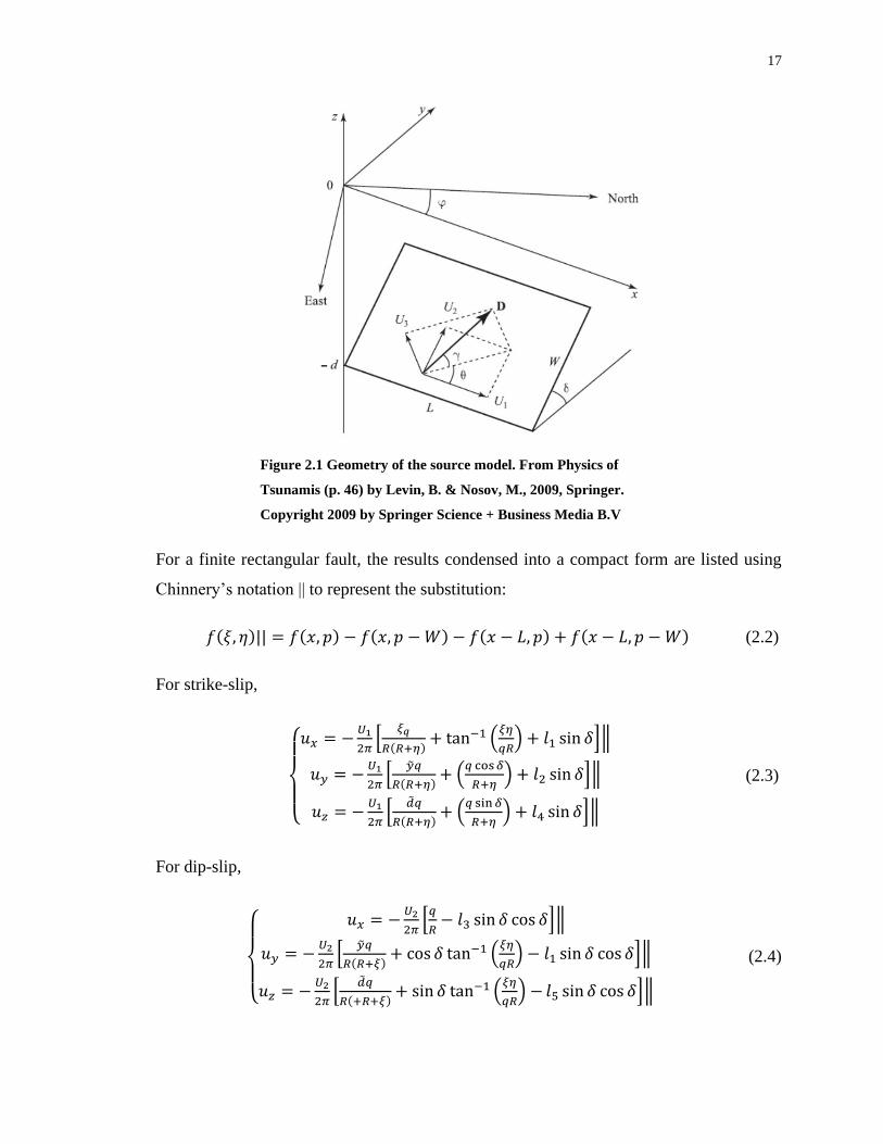
The Okada (1985) formulae are the preferred method to calculate the displacements 𝑢𝑖 in
three directions i.e. horizontal displacements 𝑈1, 𝑈2 and vertical displacement 𝑈3 (Figure
2.1). They can be used to evaluate the displacement at an arbitrary point on the surface or
inside the semi-infinite elastic medium due to a finite-fault source analytically. In this
method, the earthquake is regarded as the rupture of a single fault plane with a set of
physical parameters (dip, strike, rake, width, length, and depth).
The parameters that determine this displacement are the strike angle (represented by the x
axis in Figure 2.1), the dip angle (𝛿), rake angle (𝜃), the angle γ between the Burger’s vector
(𝐷 = 𝑈1, 𝑈2, 𝑈3), and the fault plane (W, L). In Figure 2.1, each vector (𝑈1, 𝑈2, 𝑈3)
represents the movement of the hanging-wall side relative to the foot-wall side (D) and is
related to D as: 𝑈1 = |𝐷|𝑐𝑜𝑠𝛾 ∙ 𝑐𝑜𝑠𝜃, 𝑈2 = |𝐷|𝑐𝑜𝑠𝛾 ∙ 𝑠𝑖𝑛𝜃, 𝑎𝑛𝑑 𝑈3 = |𝐷|𝑠𝑖𝑛𝛾.
(2.1)
Figu
re
2.1
Geo
metr
y of
the
sour
ce
mod
el.
Fro
m
Phys
ics
of
Tsun
amis
(p.
46)
by
Levi
n, B.
&
Nos
ov,
M.,
2009
17
For a finite rectangular fault, the results condensed into a compact form are listed using
Chinnery’s notation || to represent the substitution:
𝑓(𝜉, 𝜂)|| = 𝑓(𝑥, 𝑝) − 𝑓(𝑥, 𝑝 −𝑊) − 𝑓(𝑥 − 𝐿, 𝑝) + 𝑓(𝑥 − 𝐿, 𝑝 −𝑊) (2.2)
For strike-slip,
{
𝑢𝑥 = −
𝑈1
2𝜋[
𝜉𝑞
𝑅(𝑅+𝜂)+ tan−1 (
𝜉𝜂
𝑞𝑅) + 𝑙1 sin 𝛿]‖
𝑢𝑦 = −𝑈1
2𝜋[
�̃�𝑞
𝑅(𝑅+𝜂)+ (
𝑞 cos𝛿
𝑅+𝜂) + 𝑙2 sin 𝛿]‖
𝑢𝑧 = −𝑈1
2𝜋[
�̃�𝑞
𝑅(𝑅+𝜂)+ (
𝑞 sin𝛿
𝑅+𝜂) + 𝑙4 sin 𝛿]‖
(2.3)
For dip-slip,
{
𝑢𝑥 = −
𝑈2
2𝜋[𝑞
𝑅− 𝑙3 sin 𝛿 cos 𝛿]‖
𝑢𝑦 = −𝑈2
2𝜋[
�̃�𝑞
𝑅(𝑅+𝜉)+ cos 𝛿 tan−1 (
𝜉𝜂
𝑞𝑅) − 𝑙1 sin 𝛿 cos 𝛿]‖
𝑢𝑧 = −𝑈2
2𝜋[
�̃�𝑞
𝑅(+𝑅+𝜉)+ sin 𝛿 tan−1 (
𝜉𝜂
𝑞𝑅) − 𝑙5 sin 𝛿 cos 𝛿]‖
(2.4)
Figure 2.1 Geometry of the source model. From Physics of
Tsunamis (p. 46) by Levin, B. & Nosov, M., 2009, Springer.
Copyright 2009 by Springer Science + Business Media B.V

18
For tensile fault,
{
𝑢𝑥 =
𝑈3
2𝜋[
𝑞2
𝑅(𝑅+𝜂)− 𝑙3sin
2𝛿]‖
𝑢𝑦 =𝑈3
2𝜋[−�̃�𝑞
𝑅(𝑅+𝜉)− sin 𝛿 {
𝜉𝑞
𝑅(𝑅+𝜂)− tan−1 (
𝜉𝜂
𝑞𝑅)} − 𝑙1sin
2𝛿]‖
𝑢𝑧 =𝑈3
2𝜋[
�̃�𝑞
𝑅(𝑅+𝜉)+ cosδ {
𝜉𝑞
𝑅(𝑅+𝜂)− tan−1 (
𝜉𝜂
𝑞𝑅)} − 𝑙5sin
2 𝛿]‖
(2.5)
where
{
𝑙1 =
𝜇
𝜆+𝜇[−1
cos𝛿
𝜉
𝑅+�̃�] −
sin𝛿
cos𝛿𝑙5
𝑙2 =𝜇
𝜆+𝜇[− ln(𝑅 + 𝜂)] − 𝑙3
𝑙3 =𝜇
𝜆+𝜇[
1
cos𝛿
�̃�
𝑅+�̃�− ln(𝑅 + 𝜂)] +
sin𝛿
cos𝛿𝑙4
𝑙4 =𝜇
𝜆+𝜇
1
cos𝛿[ln(𝑅 + �̃�) − sin 𝛿 ln(𝑅 + 𝜂)]
𝑙5 =𝜇
𝜆+𝜇
2
cos𝛿tan−1 (
𝜂(𝑋+𝑞 cos𝛿)+𝑋(𝑅+𝑋) sin𝛿
𝜉(𝑅+𝑋)cos𝛿)
(2.6)
If cos (δ) = 0,
{
𝑙1 = −
𝜇
2(𝜆+𝜇)
𝜉𝑞
(𝑅+�̃�)2
𝑙3 =𝜇
2(𝜆+𝜇)⌊𝜂
𝑅+�̃�+
�̃�𝑞
(𝑅+�̃�)2 − ln(𝑅 + 𝜂)⌋
𝑙4 = −𝜇
𝜆+𝜇
𝑞
𝑅+�̃�
𝑙5 = −𝜇
𝜆+𝜇
𝜉 sin𝛿
𝑅+�̃�
(2.7)
{
𝑝 = 𝑦 cos 𝛿 + 𝑑 sin 𝛿𝑞 = 𝑦 sin 𝛿 − 𝑑 cos 𝛿�̃� = 𝜂 cos 𝛿 + 𝑞 sin 𝛿
�̃� = 𝜂sin 𝛿 − 𝑞 cos 𝛿
𝑅2 = 𝜉2 + 𝜂2 + 𝑞2 = 𝜉2 + �̃�2 + �̃�2
𝑋2 = 𝜉2 + 𝑞2
(2.8)
Okada (1985) solutions are used for horizontal bottom deformation. In slope gradients of
less than 1/3, the tsunami generation is dominated by the vertical motion of water, and the
horizontal motion of water is negligible (Iwasaki, 1982). However, if an earthquake
happens on a steep slope (continental or coastal slopes) and the horizontal displacements

19
due to faulting are relatively large and cause the slope to shift, the effects become
significant and must be accounted for (Tanioka & Satake, 1996). Hence, the vertical
displacement of water due to the horizontal movement of the slope (𝑢ℎ) is calculated as:
𝑢ℎ = 𝑢𝑥𝜕𝐻
𝜕𝑥+ 𝑢𝑦
𝜕𝐻
𝜕𝑦 (2.9)
The resulting displacement is then applied to generate the initial tsunami wave
instantaneously or over a specified rupture time. Static tsunami generation assumes the
earthquake (vertical deformation of the ocean bottom) to occur instantaneously, assuming
that the phase speed of the tsunami is slower than the propagation velocity of the earthquake
rupture. Some simulations use dynamic rupture models for an evolutionary tsunami
generation process, using frictional parameterizations and fault stress distributions (Geist
et al., 2014). Dynamic tsunami generation is usually done for ruptures of great length (i.e.
2004 Sumatra earthquake).
After the tsunami generation, the second step in tsunami simulation is the tsunami
propagation across the ocean. Tsunami waves are formed after the release of a large amount
of energy, in this case, an earthquake. The released energy is transferred to the water
column in the form of waves that have wavelengths on the order of hundreds of kilometres
(fault size = wavelength) and small amplitudes on the order of 1 m in deeper portions (water
depth = amplitudes). Thus, tsunami waves typically have a ratio of water depth to
wavelength of at least 1:20 (𝜆 ≫ 𝐻 where λ is the wavelength and H is the depth; Levin &
Nosov, 2009). As the tsunami waves move along the ocean, they lose very little energy at
greater depths, because of the great difference between wavelength and water depth,
allowing them to preserve most of their energy while travelling. Thus, tsunamis can travel
great distances. However, as the tsunami approaches shallow depths, it starts to slow down
since the wave speed depends mainly on the depth of the water (𝑐 = √𝑔𝐻 where g is
gravitational acceleration). As the tsunami front velocity decreases, the wavelength
becomes shorter because the tail of the tsunami catches up with the slower front and
increases the waves’ amplitudes. The energy is then transferred into potential energy
following the conservation of energy, and as the wave continues to slow down, it eventually

20
breaks. A part of the tsunami is reflected back to the ocean, while the remaining part
inundates the land.
The propagation of the waves is carried out in two surface dimensions over varying depth
and distances. Tsunami waves are long waves; therefore, the shallow-water theory is valid
when the wavelength is larger than the water depth. In tsunami simulations, the vertical
accelerations are negligible compared to the gravitational acceleration and curvature
trajectories. Thus, the vertical motion does not affect the pressure distribution, and the
pressure is assumed to be hydrostatic and, therefore, a linear function of depth. The
following equations further explain this:
𝜕𝑢
𝜕𝑡+ 𝑢
𝜕𝑢
𝜕𝑥+ 𝜈
𝜕𝑢
𝜕𝑦+ 𝑔
𝜕Ƞ
𝜕𝑥+𝜏𝑥
𝜌= 0 (2.10)
𝜕Ƞ
𝜕𝑡+𝜕[𝑢(ℎ+Ƞ)]
𝜕𝑥+𝜕[𝜈(ℎ+Ƞ)]
𝜕𝑦= 0 (2.11)
𝜕𝜈
𝜕𝑡+ 𝑢
𝜕𝜈
𝜕𝑥+ 𝜈
𝜕𝜈
𝜕𝑦+ 𝑔
𝜕Ƞ
𝜕𝑦+𝜏𝑦
𝜌= 0 (2.12)
where x and y are the two horizontal directions, respectively, g is the scalar vertical
acceleration due to gravity, h is the height relative to the mean ocean depth, t is time, η is
the vertical displacement, u and v are the water particle velocities in the x and y directions,
respectively, 𝜏𝑥𝜌⁄ and
𝜏𝑦𝜌⁄ are the bottom frictions in both x and y directions. The bottom
friction is expressed as an analogy to the uniform flow as:
𝜏𝑥
𝜌=
1
2𝑔
𝑓
𝐷𝑢√𝑢2 + 𝑣2 ,
𝜏𝑦
𝜌=
1
2𝑔
𝑓
𝐷𝑣√𝑢2 + 𝑣2 (2.13)
where 𝐷 = ℎ + 𝜂 is the total water depth, f is the friction coefficient which can be described
by using n is Manning’s roughness coefficient. n depends on roughness of the bottom
surface and is expressed as:
𝑛 = √𝑓𝐷1/3
2𝐺 (2.14)
Finally, the bottom friction is expressed as:

21
𝜏𝑥
𝜌=
𝑔𝑛2
𝐷43⁄𝑢√𝑢2 + 𝜈2 ,
𝜏𝑦
𝜌=
𝑔𝑛2
𝐷43⁄𝜈√𝑢2 + 𝜈2 (2.15)
Typically, the Manning’s coefficient is simplified and assumed to be 0.025 s/m1/3.
Furthermore, the coast is assumed to be free of dense vegetation which in some cases might
not be applicable.
Equations (2.10) to (2.12) are not commonly used since when discretized, the equations
might not satisfy the conservation of mass. Goto et al. (1997) recommended the following
equations instead since they have no effect on the conservation of mass and satisfy the
conservation of momentum as well.
𝜕Ƞ
𝜕𝑡+𝜕𝑀
𝜕𝑥+𝜕𝑁
𝜕𝑦= 0 (2.16)
𝜕𝑀
𝜕𝑡+
𝜕
𝜕𝑥(𝑀2
𝐷) +
𝜕
𝜕𝑦(𝑀𝑁
𝐷) + 𝑔𝐷
𝜕Ƞ
𝜕𝑥+
𝑔𝑛2
𝐷73⁄𝑀√𝑀2 + 𝑁2 = 0 (2.17)
𝜕𝑁
𝜕𝑡+
𝜕
𝜕𝑥(𝑀𝑁
𝐷) +
𝜕
𝜕𝑦(𝑁2
𝐷) + 𝑔𝐷
𝜕Ƞ
𝜕𝑦+
𝑔𝑛2
𝐷73⁄𝑁√𝑀2 + 𝑁2 = 0 (2.18)
where M and N are the discharge fluxes in the x and y directions, respectively, and are
expressed as:
𝑀 = 𝑢(ℎ + 𝜂) = 𝑢𝐷 , 𝑁 = 𝑣(ℎ + 𝜂) = 𝑣𝐷 (2.19)
The non-linear shallow-water equations allow the effective propagation analysis of the
tsunami waves that increase the resolution in the wave height as the tsunami approaches
the shore. In the deeper parts of the ocean, the linear long-wave theory gives good results
since bottom friction does not influence tsunami propagation. However, as the depth
decreases, the equations should switch to a shallow-water theory with bottom friction.
Shallow-water equations are suitable for simulating maximum run-up and inundation;
however, they are not sufficient to estimate wave forces (Shuto, 1991). In addition, as the
distance of propagation increases, Earth’s curvature and Coriolis effect should be
incorporated into the tsunami propagation model.
As the tsunami approaches the coast tsunami amplitudes increase, which determines the
danger of the tsunami to coastal communities. The increase in amplitude is due to the

22
compression of the wave train in space as the wave propagation velocity decreases due to
a decrease of depth (Levin & Nosov, 2009). This increase of height leads to the third step,
which is the tsunami shoaling, inundation, and run-up over the coastlines. Tsunami
interaction with the coastal zone has been one of the most challenging problems relevant
to tsunami dynamics. There are three types of run-up along the coast: First is spilling,
characterized by the breaking of the wave’s crest, and flowing down the frontal slope and
is particular to gently sloping bottoms. The second type is plunging which happens when
the wave’s crest surpasses foot and curls down; this type is particular to inclined bottom
slopes. Finally, the third type is surging, which is the most common type, the wave floods
the coast without breaking, particular to steep slopes.
Most models describe the wave dynamics in the coastal zone by using the non-linear
shallow-water equations (Equations 2.17-2.19). Since, as the tsunami wave approaches the
coast, the amplitudes may be proportional to the depth (Levin & Nosov, 2009). Therefore,
run-up is considered only in non-linear computations (Goto et al., 1997). The shallow water
equations can then lead to the wave speed equation: √𝑔𝐷 from which a variety of
conclusions can be drawn based on geometrical optics since wave refraction happens as the
tsunami travels around different morphology (Geisler, 2008). This interaction of the
tsunami with the surrounding topography highlights the importance of detailed knowledge
of bathymetry and elevation in the zone of interest.
Moreover, the shallow water equations can help determine boundary conditions for the
tsunami inundation simulations. Generally, during run-up simulations, the initial water
Figure 2.2 Formulation of the problem of a tsunami run-up on the coast (Levin & Nosov, 2009)
𝜂

23
level is equal to the ground height, and a widespread boundary condition, the ‘vertical wall
approximation,’ for tsunami run-up is used. This approximation imitates the continental
slope (Figure 2.2). Therefore, the tsunami run-up is modelled considering a slope connected
with a smooth horizontal ocean bottom. However, this is a considered a idealistic situation
and it is not necessarily guaranteed when realistic tsunami simulations using bathymetry
data are considered. Furthermore, the run-up can be modelled by a moving boundary
approach where the computational cell’s dry/wet is determined based on the total water
depth relative to the elevation following the expression: 𝐷 = ℎ + 𝜂 > 0, then the cell is
submerged, whereas 𝐷 = ℎ + 𝜂 ≤ 0 the cell is dry. When coastal structures are modelled,
the discharge overflowing the structure should be incorporated explicitly in the simulations.
There are some difficulties in run-up simulations to have realistic results. The first difficulty
is the quality of the bathymetry and topographical data. The necessity of having detailed
datasets comes from the fact that there is a significant reduction of the tsunami wave’s
wavelength in shallow-water zones and the influence of topographic features in the
interaction of the waves with the coast. The second difficulty is the availability and quality
of run-up measurements of past events in the area of interest, in addition to water flow
parameters information. The third is the inclusion of coastal structures in tsunami
simulations. Finally, the fourth difficulty is the erosion that tsunamis waves can cause since
that can change the aspect of the coast (i.e., demolition of buildings and destruction of
vegetation) and how the waves will interact with the coast.

24
Chapter 3
3 Stochastic Source Modelling and Tsunami Analysis of the
2012 Mw 7.8 Haida Gwaii Earthquake
On October 28th, 2012, off the western coast of Moresby Island (Figure 3.1) an Mw 7.8
earthquake occurred on a thrust fault beneath the Queen Charlotte Terrace (QCT) beneath
the Queen Charlotte Fault (QCF). The earthquake was the second largest instrumentally
recorded in the region after the 1949 Mw 8.1 earthquake. The 2012 earthquake triggered a
tsunami that was recorded all along the Pacific Ocean. On the northwestern Pacific, the
tsunami was recorded on tide gauges, bottom pressure recorders and deep-ocean buoys.
Furthermore, coseismic deformation measurements were obtained during the consequent
months by GPS stations (Nykolaishen et al., 2015) and intertidal biological organisms level
measurements (Haussler et al., 2015). The tsunami run-up was measured by field surveys
(Leonard & Bednarski, 2014). Multiple past studies have constrained the source fault using
different methods. In the present chapter, a tsunami analysis of the Haida Gwaii region
using stochastic source modelling and Monte Carlo tsunami simulation is conducted to
develop stochastic source models that generate tsunami waves in close match with the
recorded observations. The methodology involves the synthesis of stochastic sources
constrained by deformation measurements, aftershock sequences, and thermal
measurements. The synthesized source models are then used in Monte Carlo tsunami
simulations with run-up to simulate the tsunami waves at different offshore and offshore
locations.
The chapter is organized as follows: First, an overview of the 2012 Haida Gwaii event; and
the region’s seismicity and tectonics. Secondly, the finite fault models from the literature
are presented. Thirdly, the methodology for evaluating the existing source models, the
stochastic source modelling, and Monte Carlo tsunami simulation for the present study is
explained in detail. Finally, the results of the tsunami analysis of the 2012 earthquake are
explained in detail for offshore and onshore observations.

25
3.1 2012 Haida Gwaii Event
At 8:04 P.M Pacific daylight time on October 28, 2012, an Mw 7.8 earthquake hit the region
of Haida Gwaii, British Columbia, Canada (Figure 1.1). The perceived shaking in the Haida
Gwaii Islands lasted between 1.5 to 2 minutes, with strong shaking for about 30 seconds
(Bird & Lamontagne, 2015). The earthquake was felt throughout British Columbia, and
some accounts indicated that it reached as far as Yukon, Alberta and Montana (Bird &
Lamontagne, 2015). Due to the far distance between the epicentre and the populated areas,
this earthquake resulted in minimal residential house damages in the region (Bird &
Lamontagne, 2015). In addition, the epicentre was close to other thrust events of the zone,
such as the 2001 Mw 6.2 earthquake south of the QCF (Lay et al., 2013).
The 2012 earthquake nucleated below the western coast of Moresby Island. However, most
of the slip occurred 20 km off the coast of Haida Gwaii at a depth of 23 km, below the
sedimentary wedge, and about 230 km north of the triple junction between the Explorer,
Figure 3.1 a) location of the thrust fault beneath the QCT in which the 2012 earthquake occurred, the
relative plate motions in this area, and location of the near-vertical QFC (Cassidy et al., 2014). (b)
Surface temperatures, two possible geometries of
26
Pacific, and North American Plates (Lay et al., 2013, Bird & Lamontagne, 2015, Haeussler
et al., 2015; see Figure 3.1a). The United States Geologic Survey (USGS) reported a fault
area of about 140 km by 30 km. In comparison, Kao et al. (2015) reported fault area
dimensions of ~120 km by 30 km based on the epicentre location and the aftershock’s
spatial distributions. The mainshock’s epicentre was located at 52.622°N, 132.103°W, at a
depth of 14 km (Kao et al., 2015). Ground motions with the highest amplitudes were
observed on the western coast of Moresby Island, in Masset and Prince Rupert (Figure 1.1),
and reached the maximum horizontal accelerations of 0.2 g in the region (Leonard &
Bednarski, 2014, Bird & Lamontagne, 2015, Barth et al., 2020). After the mainshock,
thousands of aftershocks followed, the largest being an Mw 6.3 event on October 28, 2012,
and an Mw 6.1 event in October 2019 (Cassidy et al., 2014, Barth et al., 2020; see Figure
3.1c).
Global Positioning System (GPS) data indicated southwestward coseismic surface
displacement of 3 to 115 cm on the western coast of Moresby Island. In addition, seismic
waveforms, aftershocks, and coseismal deformation from GPS measurements indicated
that the earthquake had a low angle thrusting motion, with a slip partitioning in the
transgressive boundary (James et al., 2013, Lay et al., 2013, Kao et al., 2015, Nykolaishen
et al., 2015). This was consistent with the coseismic offset expected from an offshore
shallow-thrust earthquake (Cassidy et al., 2014, Nykolaishen et al., 2015). Moreover, the
shallow angle of the 2012 Mw. 7.8 Haida Gwaii earthquake confirmed oblique convergence
and underthrusting (James et al. 2013, Cassidy et al. 2014). Lay et al. (2013) performed a
series of teleseismic P-wave seismic inversions and estimated the earthquake rupture
parameters, such as fault dimensions, rupture velocity, and dip and hypocentre, by fitting
their simulations with the observations at DART buoys. The P-wave projection imaging
indicated a non-uniform rupture expansion toward the southeast and northwest. Leonard et
al. (2014) calculated a recurrence rate of ~ 760 years for Mw 7.7 strike-slip earthquakes
based on the convergence rate and the average earthquake slip.
The tsunami triggered by the earthquake was recorded on tide gauges, Bottom Pressure
Recorders (BPRs) by Ocean Canada’s Neptune network and Deep-ocean Assessment and
Reporting of Tsunamis (DART) buoys across the Pacific Ocean (Figure 3.2). Horizontal

27
and vertical deformations were also obtained using GPS measurements (Nykolaishen et al.,
2015) and intertidal biological indicators (Haeussler et al., 2015). Moreover, the run-up
level was defined by natural and artificial ocean debris and reached more than 7 m at
locations like Mike Inlet in Moresby Island (James et al., 2013, Lay et al., 2013, Leonard
& Bednarski, 2014; see Figure 3.8). Leonard et al. (2014) predicted that events of the
magnitude of the 2012 earthquake could yield run-ups of 3–7 m for coastlines within 40
km of the rupture zone.
3.2 Tectonics and Seismicity of the Haida Gwaii Region
The QCF is a primarily right-lateral transform fault boundary of the Pacific and North
American Plates. It extends more than 800 km from the triple junction north of Vancouver
Island to the Alaskan Subduction Zone (Cassidy et al., 2014, Hyndman, 2015). Towards
southern Alaska, the QCF becomes the Fairweather Fault (Walton et al., 2013). To the
north, the QCF strikes at 338º and is mainly a transform fault plate boundary with ocean
crust seaward and continental crust landward (Cassidy et al., 2014). Most earthquakes in
the northern region, have occurred in the vertical QCF parallel to the Pacific-North
American Plate’s motion, with a nearly pure strike-slip rupture as mechanism (Hyndman,
2015). The south of the QCF is marked by the triple junction of the Pacific-North
American-Explorer plate and a slow margin convergence known as the Winona basin
(Hyndman, 2015, Kao et al., 2015).
Margin Convergence and Underthrusting
Before the 2012 earthquake, there had been evidence of subduction in the region, later
confirmed by the 2012 earthquake. The evidence included: gravity and heat flow data, the
existence of a bathymetric trench and accretionary prism, and receiver-function analyses
showing dipping oceanic slab (Leonard & Bednarski, 2014).
Hyndman (2015) further explains the oblique convergence accommodated by
underthrusting by the following factors:
1. An offshore ocean plate fore bulge, which is characteristic of subduction
underthrusting.
2. A trough with characteristics of a subduction trench.

28
3. The QCT appears to be a compressive sedimentary fold and thrust belt.
4. The gravity pattern across the margin has a linear low over the Queen Charlotte
trough and terrace and large highs over the western coast of the islands.
5. The heat flow pattern across the margin and the offshore high head decreases
landward under the terrace.
6. Landward-dipping boundaries are interpreted to delineate the underthrust.
7. GPS-derived displacement vectors on the islands are oriented 10° to 30°clockwise
from the margin trend.
8. The uplift in the western coast of the islands and the high and steep topography
along the western coast of Haida Gwaii are the result of the oblique convergence
(Motazedian et al., 2016).
In addition to the factors stated above, the plate motion kinematics in the QCF match the
down-dip transition of the seismogenic behaviour of the megathrust, which is thermally
controlled. The landward part of the QCF accommodates the oblique motion of the oceanic
plate beneath the continental crust and exhibits creep (Wang et al., 2015; see Figure 3.1b).
While the seaward shallow thrust accommodates the normal component relative to the plate
motion, noting that this portion produced the 2012 Haida Gwaii earthquake, and the QCF
accommodates the strike-slip component. Lastly, the recurrence period for this type of
earthquake might be 760 years, assuming thrusting and no creeping in the plate
convergence (Leonard et al., 2014).
Fault Geometry
The complexity of the evolving triple junction with the Explorer Plate and the changes in
relative motion between the Pacific and North America Plates make it difficult to constrain
the regional plate boundaries (Lay et al., 2013). Rohr (2015) identified that the northern
part of the Revere-Dellwood Fault zone overlaps the southern end of the QCF and is close
to the southmost extent of the 2012 thrust earthquake, which might be the southern limit of
the main underthrusting. Furthermore, coseismic subsidence on the western coast of Haida
Gwaii suggested that the main rupture did not extend landward from the QCF (Nykolaishen
et al., 2015). Based on coseismic subsidence and arrival times at local seismograph stations,
Kao et al. (2015) suggested a relocated position for the epicentre 5 km further seaward,

29
which implies that the Haida Gwaii mainshock was near the bottom of the seismogenic
interface. The aftershock distribution also indicated that the earthquake ruptured mainly
offshore with a limited extension landward just under the coast (Hyndman, 2015).
Moreover, the lack of aftershocks down-dip landward and thrust-aftershocks might also
indicate that the total stress was located on the shallow part of the thrust plane (Lay et al.,
2013; see Figure 3.1).
GPS data recorded 30 cm subsidence on the southern part of Moresby Island, further
implied that the rupture was entirely offshore (Nykolaishen et al., 2015). The aftershock
distributions defined a rupture zone area of ~150 km in length and a width of 30 km (about
the width of the QCT). The width of the fault is constrained by thermal models, which
suggest a landward limit of the rupture (Cassidy et al., 2014, Kao et al., 2015, Wang et al.,
2015). Furthermore, thermal constraints of the potential seismogenic zone as well as the
kinematics of the slip partitioning, which is predominantly orthogonal to the margin,
assume that the Haida Gwaii rupture was limited mainly updip of the intersection of the
thrust fault with the QCF (Cassidy et al., 2014, Nykolaishen et al., 2015, Wang et al., 2015).
In addition, there have not been thrust events associated with the plate interface in the
landward part of the QCF (Wang et al., 2015). The Global Centroid Moment Tensor Project
reports this event as a shallow thrust mechanism with strike = 318°, dip = 25°, and rake =
104° (Nykolaishen et al., 2015).
3.3 Observations
The 2012 Haida Gwaii earthquake generated a tsunami that was recorded on Fisheries and
Ocean Canada (FOC) tide gauges throughout the Haida Gwaii Islands, Vancouver Island,
and the mainland. In addition, NEPTUNE, Ocean Network Canada (ONC) bottom pressure
sensors (BPRs) recorded the event along southwestern Vancouver Island (Leonard and
Bednarski, 2014, Fine et al., 2015). On the American side, the 2012 tsunami event was
recorded at National Oceanic and Atmospheric Administration (NOAA) tide gauges; at
least 110 instrumental records of this event are located on the NOAA tsunami database
(Fine et al., 2015). Across the Pacific Ocean, Deep-ocean Assessment and Reporting of
Tsunami (DART) stations recorded the event (Figure 3.2). Deformation was also measured
along the main island in the months following the earthquake by GPS measurements

30
(Nykolaishen et al., 2015) and biological intertidal indicators (Haussler et al., 2015). In
addition, Leonard and Bednarski (2014) conducted field surveys to measure the tsunami
run-up along bays and inlets several weeks after the earthquake. Therefore, the 2012 Haida
Gwaii event was well documented, providing important information for the validation of
tsunami simulations, which can help constrain the source parameters for possible future
events in the zone.
Figure 3.2 Map of Haida Gwaii showing the locations of FOC and NOAA tide gauges, Ocean Network
Canada BPRs and DART buoys that recorded the 2012 Haida Gwaii tsunami

31
Deformation
The horizontal and vertical deformations of the 2012 Haida Gwaii earthquake were
recorded using GPS measurements in the following months after the event (Table 1.1).
Nykolaishen et al. (2015) investigated the coseismic and postseismic displacements at a
series of GPS stations along Moresby Island, southern Haida Gwaii (Figure 3.3). However,
there was only one continuously operating GPS station (BCSS) about 80 km from the
epicentre in the region. Therefore, to complement this station and monitor the aftershock
sequences, a set of GPS stations along temporary seismic stations was placed in the Haida
Gwaii region two weeks after the earthquake by the Geological Survey of Canada (GSC)
of Natural Resources Canada (NRCan; James et al.2013). The results show a coseismic
displacement of 22 cm in the south-southwest part of the Haida Gwaii for the continuously
GPS station (BCSS) with horizontal deformations ranging from 3 cm to 115 cm, whereas
the vertical deformations showed subsidence of 1 cm to 30 cm (except for BCPR that
presented uplift). The site (BARI) closest to the epicentre (30 km) recorded a coseismic
displacement of 115 cm to the south-southwest and subsidence of 30 cm (Figure 3.3a). The
cumulative postseismic horizontal displacements for seven GPS sites were up to 6 cm over
one year (Nykolaishen et al., 2015). The results suggest that multiple processes might be
involved, like long-term processes that might include elastic deformation that did not
contribute to the coseismic displacement during the earthquake and started a few days after
the earthquake indicating an aseismic after-slip of the deeper portion of the fault beneath
Moresby Island.
Table 3.1 Coseismic offsets at GPS stations in the Haida Gwaii region
Site Longitude° Latitude° dN (cm) dE (cm)
dHGHT
(cm)
BCPR -130.435 54.277 -0.024 -0.013 0.007
YAKA -131.837 54.071 -0.052 -0.026 -0.011
BCSS -131.808 53.254 -0.19 -0.104 -0.007
NCRS -131.960 53.144 -0.283 -0.15 -0.06
MORE -132.087 53.020 -0.482 -0.262 -0.107
BARI -131.753 52.5766 -0.931 -0.682 -0.303
STJA -131.016 51.937 -0.068 0.019 -0.054 dH, north component offset; dE, east component offset, dHGHT, vertical component offset

32
The vertical coseismic deformations (Figure 3.3b) were also measured by the upper growth
limits of two intertidal organisms (rockweed and barnacle) at 25 different sites on the
western coast of Moresby Island (Haussler et al., 2015). The mean elevations of the
organism with respect to the mean sea level were evaluated by a linear fit to find the vertical
deformation. Lower elevations between the organism and the mean sea level were
correlated to subsidence after the earthquake. The results show coseismic subsidence of
around 40 cm to 60 cm along the entire western coast. There are also differences in
elevation between the upper limits of each organism in the northern and southern parts,
with decreasing elevations from north to south. Lower elevations were measured in the
rupture region. These lower values in the south of the island were consistent with the GPS
measurements in the southern part of the Haida Gwaii region.
Figure 3.3 a) Horizontal deformation by GPS measurements. b) vertical deformation by intertidal
biological indicators and GPS measurements

33
Tide Gauges
The tsunami waves were recorded on FOC and NOAA tide gauges scattered throughout the
Pacific Ocean (Figure 3.2). Eleven FOC tidal stations recorded the tsunami waves around
British Columbia (BC), with nine Permanent Water Level Network (PWLN) stations and
two temporary stations. All FOC stations exposed on the BC western coast recorded
tsunami amplitudes, including some onshore locations, such as Queen Charlotte. The
tsunami signals at FOC stations had a sampling rate of 1 minute (Figure 3.4).
NOAA stations recorded amplitudes at coastal locations in Alaska, California, Oregon,
Washington, and Hawaii. High amplitudes were recorded away from the source at stations
in Hawaii, and smaller amplitudes were recorded north of the rupture zone (i.e., Ketchikan;
Figure 3.4). While the highest amplitudes were recorded on stations south of the rupture
(i.e., Port Orford, Crescent City, Figure 3.4). The tsunami signals for NOAA stations had a
sampling rate of 6 minutes.
Figure 3.4 Time histories of the 2012 Haida Gwaii tsunami waves at FOC and NOAA tide gauges

34
In this study, only stations close to the rupture area are analyzed. The stations were further
scrutinized by the data quality, wave periods, wave amplitudes, and distances to the source
area (4 FOC and 4 NOAA stations). The tidal records were processed to extract the tsunami
wave amplitudes from the time series. The tidal records were processed using a Butterworth
high-pass filter to attenuate low-frequency signals associated with tidal atmospheric
processes. Since the records had different sampling rates, the signals were resampled to a
sampling rate of 1 second, respecting the Nyquist frequency. Despite the earthquake’s
magnitude, the amplitudes recorded at the chosen stations (Figure 3.2) were relatively
small. Fine et al. (2015) noted that the low amplitudes are related to the directivity of the
tsunami source region, which radiated the tsunami energy in an offshore direction, and the
shadowing effect of Haida Gwaii. The maximum amplitudes were recorded on Henslung
Cove (28 cm) and Winter Harbour (20 cm). Furthermore, it is also important to note that
the region’s topography is constituted mainly of fjords and cliffs, which can shield the
stations from the tsunami waves. The travel path can also explain these low amplitudes
since the tsunami waves had to travel around the southern and northern tips of Haida Gwaii
to reach some of the stations. The time arrivals of the first tsunami wave at different stations
ranged between 1 and 3 hours after the earthquake (Table 3.2).
Table 3.2 Wave parameters of the October 28, 2012 Haida Gwaii tsunami derived from tide gauge
observations on the northwestern Pacific
Stations First Wave
Arrival Time
(UTC) Maximum Amplitude (m)
Winter Harbour (FOC) 4:13 0.18
Queen Charlotte (FOC) 5:42 0.04
Henslung Cove (FOC) 3:52 0.13
Tofino (FOC) 4:49 0.09
Ketchikan (NOAA) 4:54 0.018
La Push (NOAA) 5:00 0.09
Port Orford (NOAA) 5:24 0.11
Crescent City (NOAA) 5:48 0.14

35
Deep-Ocean Observations
Deep-sea observations were recorded on both ONC BPRs and DART stations (Figure 3.5).
ONC BPRs located to the west of Vancouver Island had the highest resolution and highest
sampling rate at 1 second. While the DART stations had a standard sampling rate of 15
minutes, that switched into a 1-minute sampling mode at the time of the earthquake and
then switched back to the standard 15-minute sampling rate. The tsunami signals for both
ONC and DART records were filtered with a high-pass filter. Since the DART stations had
different sampling rates, the signals were re-sampled to 1-second intervals to match the
sampling rate of the other observation stations. Three out of the four ONC BPRs were
picked based on data quality and the amount of background noise present. The three stations
are located on the shelf, continental slope, and in deep water. Five DART stations were
chosen for the present study based on data quality and distance from the source. The closest
stations to the source zone were picked due to the limitations of the tsunami simulation
code, and the present bathymetry of the northern regions, which presented clear distortion
in the Alaska region.
Figure 3.5 Time histories of the 2012 Haida Gwaii tsunami waves at ONC's BPRs and DART buoys

36
The recorded tsunami amplitudes were relatively small due to the stations not being located
directly in the tsunami propagation path. The highest amplitudes were recorded at stations
DART 46407 and DART 46419 (Figure 3.5, Table 3.3). Furthermore, both observations
had relative low background noises since they are not affected by coastal effects in
comparison to the coastal tide gauges (Fine et al., 2015); thus, deep-sea observations
provide accurate tsunami waves information.
Table 3.3 Wave parameters of the October 28, 2012 Haida Gwaii tsunami derived from deep-sea
observations on the northwestern Pacific
Stations First Wave
Water
Depth (m) Arrival Time (UTC) Maximum
Amplitude (m)
Clayoquot Slope 1258 4:22 0.05
Barkley Canyon 392 4:57 0.07
Cascadia Basin 2660.5 4:34 0.02
DART 46404 3738 5:34 0.05
DART46407 3300 3:49 0.07
DART46410 3755 4:05 0.03
DART 46411 4325 4:14 0.03
DART 46419 2795 4:06 0.04
Run-up Observations
Leonard and Bednarski (2014) conducted the post-tsunami field surveys, obtaining the
near-field observations. Unfortunately, the lack of eyewitness accounts, the limited
accessibility of the terrain, and the fact that the Haida Gwaii region is prone to large storms
made post-tsunami surveys difficult to carry out. Thus, the run-up data were limited to a
small number of sheltered bays and heads of long inlets (Leonard & Bednarski, 2014, Fine
et al., 2015). The run-up was measured based on disturbed forest floor, evident erosion,
depositional evidence, and natural or manmade debris with a clear oceanward origin
(Figure 3.6). The run-up sites were divided into two categories. The first was sites that were
exposed to storm waves; these sites had the larger measured run-up. The second was sites
sheltered from storms, where smaller values were observed (Table 3.4). The maximum run-
up at sites open to storm waves was 13 m at Davison Inlet, whereas the maximum measured
run-up in sheltered from storm waves sites was 7.6 m at Mike Inlet.

37
Table 3.4 Tsunami runup and inundation data of the 2012 Haida Gwaii tsunami
Sites Run-up (m) Inundation from shore(m)
Sites Sheltered from Storm Waves
Seal Inlet 3.6 28.5
Sunday Inlet 4.8 23.6
Pocket Inlet 5.3 29.1
Mike Inlet 6.4 22.8
Puffin Cove 3.4 5
Goski Bay 4.3 27.4
Staki Bay 3.1 25.5
Louscoone Inlet 3.7 12.8
Sites Exposed Storm Waves
Otard Bay 6.8 34.8
Gudal Bay 6.9 8.5
Saunders Island 7.3 29
Davidson Inlet 9 21.1
Kwoon Cove 6.5 5
Ta'dasl 8.1 14
Gilbert Bay 7.3 30.8
Figure 3.6 Run-up sites with colors depending on amount of run-up

38
These high tsunami run-ups might result from the natural resonant periods of the inlets that
promote wave amplification. Another plausible explanation is that before the post-tsunami
surveys, a large storm occurred in the region, possibly overprinting the tsunami evidence,
especially in the sites that were exposed to storm waves.
3.4 Inversion Models
Inversion models are an important tool in tsunami simulation analysis, as they are based on
past seismic events. These models attempt to produce close approximations of earthquake
rupture processes by combining observed data (i.e. teleseismic data, strong motion,
geodetic observations, and tsunami observations) and geophysical model predictions (Goda
et al., 2016). However, it is important to note that finite fault models have limitations due
to their resolution and robustness (Lay et al., 2013, Goda et al., 2016, Mori et al., 2018).
Nevertheless, in the literature, earthquake databases with finite fault models are vastly
available, such as SRCMOD finite-source rupture model database (Mai & Thingbaijam,
2014) and the United States Geological Survey National Earthquake Information Center
(Hayes, 2017). There are various finite fault models for the 2012 Haida Gwaii earthquake
(Table 3.5). Most of the literature models used in this study were obtained from the
SRCMOD database. Six inversion models were gathered, analyzed, and used as constraints
for the stochastic source models.
Table 3.5 Parameters of inversion models from literature
Model Length
(km)
Width
(km)
Strike, Dip,
Rake
Seismic moment
(Nm) Lay et al., (2013) 144 52 320,18.5,109 6.74x10²⁰
Wei, (2012) 210 90 319,29,112 7.00x10²⁰
Shao & Ji, (2012) 144 60 325,29,112 4.27x10²⁰
Hayes, (2013) (Fine et al.
2015) 252 82 323,30,120 7.33x10²⁰
Gusman et al., (2016) 165 60 317,18.5,103 5.30x10²⁰
Hayes, (2017) 252 82 323,30,125 7.33x10²⁰
Lay et al. (2013) used teleseismic broadband P waves and SH waves to generate a finite
fault model of the 2012 event (Figure 3.7a). The model was constrained using W-phase
solutions, information from short-period back projections, and tsunami observations off the
coast of Hawaii and DART buoys. The fault geometry, rupture velocity, and hypocentre

39
were matched to the near and far-field characteristics using DART buoys observations.
Overall, the final model matched broadband teleseismic P waves, short-period projections,
and tsunami observations near Hawaii. However, the model had some uncertainty in the
location of the hypocentre. Wei (2012) used teleseismic P waveforms and 63 SH
waveforms for the inversion model (Figure 3.7b). The data were then used to obtain the
slip distribution of the fault plane using the inversion algorithm by Ji et al. (2002), which
introduces a wavelet transform to constraint the time and frequency characteristics of the
seismic waveforms. Shao and Ji (2012) used teleseismic broadband P waveforms, SH
waveforms, and long-period surface waves for the inversion of the finite fault model
(Figure 3.7c). The data were converted to displacement, and the finite-fault inverse
algorithm (Ji et al., 2002) was used to constrain the slip distributions in the fault plane.
Similar to the Wei (2012) model, Shao and Ji (2012) only compared their finite fault model
results with the waveforms of seismographs.
Fine et al. (2015) focused on studying the near-field characteristics of the Haida Gwaii
tsunami. Tsunami observations (DART and ONC buoys) and numerical model simulations
were used to study the physical properties of the Haida Gwaii event and test the accuracy
of the inversion models present at the time. A modified version of the inversion model of
Hayes (2013) was used to define the vertical displacement in the source region (Figure
3.7d). The modelled amplitudes of the study agreed with four observations at DART
stations. However, the modelled arrival times differed from the observations. The late
arrival time of the tsunami simulations suggested that the location of the earthquake
epicentre was different from the one used by Hayes (2013). The inverse isochrones method
was used to estimate the exact location and source boundaries. The results indicated that
the actual epicentre was 23–25 km to the southeast of the original source model by Hayes
(2013). The final finite-fault model was in better agreement with GPS measurements
obtained by Nykolaishen et al. (2015). However, the study did not use fine nested grid
formulations nor high-resolution bathymetry for tsunami simulations. Thus, the study did
not present a detailed comparison between the simulated tsunamis and the observations at
each coastal station nor calculated run-up and inundation.
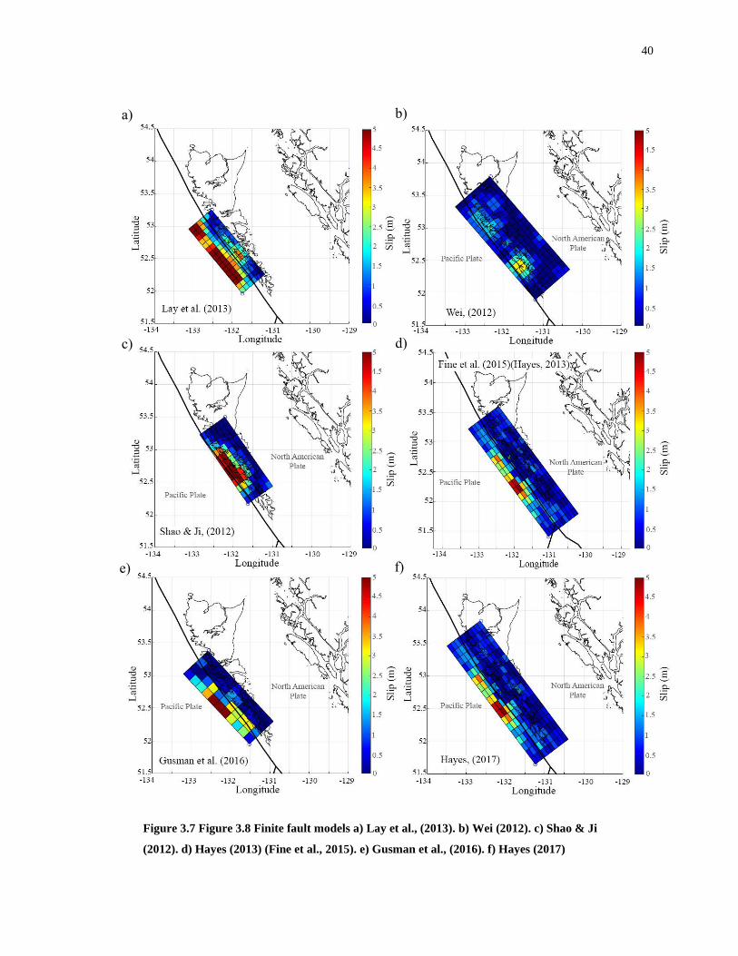
40
a) b)
c) d)
e) f)
Figure 3.7 Figure 3.8 Finite fault models a) Lay et al., (2013). b) Wei (2012). c) Shao & Ji
(2012). d) Hayes (2013) (Fine et al., 2015). e) Gusman et al., (2016). f) Hayes (2017)

41
Gusman et al. (2016) used tsunami waveforms recorded on seafloor pressure gauges off-
shore Oregon and California to test two different real-time tsunami-forecasting methods.
The first tsunami source was estimated by inversion of the recorded tsunami waveforms,
while in the second method, the data were assimilated to produce tsunami wave-fields
(Figure 3.7e). The data used were the tsunami waveforms recorded on DART buoys and
absolute pressure gauges. The model had a forecast accuracy vs the data of 94% on average
at stations near the coast, which decreased on stations further away. The study demonstrated
that tsunami records on dense pressure gauge arrays could deliver timely and accurate
forecasts on the nearby coast. However, as this study focused on early warning purposes,
the resolution of the finite fault model was coarse. The Hayes (2017) model is preferred for
the USGS studies. It used broadband teleseismic data for the inversion analysis, and the
finite fault inversion approach was that of Ji et al. (2002) (Figure 3.7f).
3.5 Earthquake Scenario
Several source models that define the Haida Gwaii region can be found in the literature.
For the present study, six finite-fault models (Section 3.4) were analyzed. The fault
boundaries of most finite-fault models were generated using tsunami data, whereas ground
motions were only used in two models (i.e. Shao & Ji, 2012, Wei, 2012). The models’
source parameters can be found in Table 3.5. The 2012 Haida Gwaii earthquake occurred
on a previously unknown thrust fault dipping to the northeast (Hobbs et al., 2015). The
strike of the rupture zone was parallel to that of the QCF. The models’ strike ranged from
317º to 325º, consistent with that of the southern segment of the fault where the earthquake
occurred. Their hypocentral depth ranged from 15 km to 18 km. The dip of the rupture zone
was not well constrained despite the seismic structure and gravity data across the margin
(Hyndman, 2015). The model’s dip angles ranged from 18º to 30º. Finally, solutions from
the Global Centroid Moment-Tensor (CMT) and USGS centroid moment tensor showed
almost pure thrust faulting with rakes of 104° and 100°, respectively. However, solutions
from Kao et al. (2015) indicated a larger oblique component with the slip vector turning
toward the north. These higher values are more compatible with the relative plate motion
of the Haida Gwaii region. Thus, the literature models presented larger rakes ranging from
109° to 125° (Table 3.5).

42
The source parameters such as the fault length (L), width (W), mean slip (Da), maximum
slip (Dm), Box-Cox parameter (λ), correlation length along strike direction (Az),
correlation length along dip direction (Ax), and Hurst number (H) are evaluated as a
function of moment magnitude using the methodology outlined by Goda et al. (2016)
(Table 3.6).
Table 3.6 Summary of the finite fault source parameters for the 2012 Haida Gwaii earthquake
First, the maximum usable wave number is defined based on the original grid resolution of
the literature models to check the slip values. Then, the subfaults with zero slips at the edge
of the fault are removed to focus on the main slip features of the original model. The slip
is evaluated using the effective width and length (Mai & Beroza, 2000).
𝑊𝐸 =∫ (𝑓𝑊∗𝑓𝑊)𝑑𝑠∞−∞
𝑓𝑊∗𝑓𝑊|𝑠=0 , 𝐿𝐸 =
∫ (𝑓𝐿∗𝑓𝐿)𝑑𝑠∞−∞
𝑓𝐿∗𝑓𝐿|𝑠=0 (3.1)
where 𝑓𝑊 and 𝑓𝐿 are the one-dimensional slip function along dip and strike, respectively.
𝑓𝑊 ∗ 𝑓𝑊 and 𝑓𝐿 ∗ 𝑓𝐿 are the auto-correlation function of the one-dimensional slip,
respectively.
Secondly, the row/ column at the fault’s edge is trimmed to find the largest dimension (W
or L) that fits the autocorrelation dimensions. The largest fitted dimension is determined,
so the difference between the dimension and the autocorrelation is less than or equal to the
subfault size. Depending on the size of the model, the effective dimensions can be smaller
than the original dimensions. Da and Dm are then evaluated using the new effective
dimensions.
Model Mw L
(km)
W
(km)
Da
(km)
Dm
(km) λ
Az
(km)
Ax
(km) H
Lay et al. (2013) 7.82 144 52 2.88 7.67 0.3 11.52 11.52 0.69
Wei (2012) 7.83 210 90 0.8 3.16 0.1 17.6 17.6 0.99
Shao & Ji (2012) 7.72 144 60 2.15 6.29 0.4 12 12 0.99
Hayes (2013)
(Fine et al. 2015) 7.83 252 82 1.12 5.6 0.3 14.28 14.28 0.61
Gusman et al.
(2016) 7.8 165 60 1.38 5.43 0.4 10.5 10.5 0.68
Hayes (2017) 7.83 238 65.6 1.12 5.61 0.3 14.28 64.26 0.61

43
Subsequently, the Box-Cox parameter is calculated using a Box-Cox transformation to
characterize the probability distribution of slip values on the fault plane and find the best
power parameter to transform a non-normal variable into a normal variable.
𝑌 =𝑋𝜆−1
𝜆(𝜆 ≠ 0) (3.2)
where X is the original variable, Y is the transformed variable, and 𝜆 is the power (Box-
Cox) parameter. When 𝜆 = 0 the Box-Cox transformation equates to the lognormal
transformation.
Finally, Az, Ax, and H are calculated using a von Karman wavenumber spectrum P(k) (Mai
& Beroza, 2002)
𝑃(𝑘) ∝𝐴𝑧𝐴𝑥
(1+𝑘2)𝐻+1 (3.3)
where k is the wavenumber and is expressed as 𝑘 = (𝐴𝑧2𝑘𝑧
2 + 𝐴𝑥2𝑘𝑥
2)0.5. Az, Ax, and H are
estimated by minimizing the difference between the observed down-dip/along-strike
spectrum and the theoretical spectrum. The H is constrained to range between 0 and 1.
Finally. a two-dimensional Fast Fourier Transform (FFT) is carried, and the amplitude
spectrum is normalized to the maximum value.
Based on the geometry of the finite-fault models, a generic fault model of the Haida Gwaii
region is defined for the synthetic source generation (Figure 3.8). The usage of various
existing models is favourable because the epistemic uncertainty of source models is
considered. The generated fault model covers the whole Haida Gwaii Islands, and its L and
W are 315 km and 95 km, respectively. The fault model’s geometry is larger than the one
predicted for the 2012 Haida Gwaii event (Table 3.6) to allow for a range of geometry for
the stochastic source models and to fit various asperity areas for different case scenarios.
The slip at the edge of the models is tapered to zero to avoid abrupt changes in slip values
at the fault boundaries (Hayes, 2017). The top edge of the fault plane is positioned at a
depth of 3 km, and the strike (325º) and dip (20º) are kept constant. The fault is discretized

44
into 5 km by 5km subfaults for the stochastic modelling and Monte Carlo tsunami
simulation.
Subsequently, the scenario moment magnitude is selected according to the objective of the
analysis. For the present study, an Mw range of 7.7-7.9 is considered. Furthermore, within
the fault model, an asperity zone is defined (Figure 3.9). The asperity zone constrains the
slip concentration within the generated source models, and its definition is not
straightforward. The asperity zone needs to accommodate a certain amount of slip that is
greater than the specified threshold within the target region and must reflect the
seismological characteristics of the region. Thus, the asperity zone must be defined
carefully based on geophysical aspects of the 2012 Haida Gwaii earthquake, such as the
aftershock sequences (Figure 3.1c). Kao et al. (2015) divided 18 strike-slip aftershocks into
four groups: the first group occurred at shallow depths near the surface trace of the QCF
with a right-lateral component. The second group occurred on secondary fault zones
adjacent to the QCF. The third group occurred within the underthrusting Pacific Plate. The
Figure 3.8 Tsunami source zone model for the Haida Gwaii region

45
final group was located directly beneath the surface trace of the QCF. All aftershocks
occurred on the southern part of Moresby Island, with depths ranging from 5 km to 25 km,
just underneath the island’s western coast.
Furthermore, the depth of the asperity zone is constrained by high temperatures of the
deeper portion that exhibit mostly creep behaviour (Wang et al., 2015). Wang et al. (2015)
estimated a depth range of 15-20 km for the depth limit of the rupture zone based on three
large strike-slip earthquakes along the fault; thus, confining the rupture zone to a shallow
down-dip area (Hyndman, 2015).
The asperity rectangle for the source models is specified as fractions of the fault length and
width. In contrast, the extent of the slip concentration around the asperity is specified as a
percentage of slip within the asperity rectangle with respect to the total sum of slip over the
Figure 3.9 Map showing the synthetic fault plane (black) and the asperity zone
(red)

46
fault plane. The slip needed to be concentrated within the asperity zone 70% to 100% for
the present scenario.
3.6 Source Parameters
After defining the earthquake scenario, fault model and asperity zone. The earthquake
source parameters (W, L, Da, Dm, Az, Ax, λ, and H) are generated as a function of Mw
using the following scaling relationship derived from global source models (Goda et al.,
2016):
log10𝑊 = −0.4877 + 0.3125𝑀𝑤 + 0.1464휀𝑊 (3.4)
log10 𝐿 = − 1.5021 + 0.4669𝑀𝑤 + 0.1717휀𝐿 (3.5)
log10𝐷𝑎 = −5.7933 + 0.7420𝑀𝑤 + 0.2502휀𝐷𝑎 (3.6)
log10𝐷𝑚 =− 4.5761 + 0.6681𝑀𝑤 + 0.2249휀𝐷𝑚 (3.7)
log10 𝐴𝑧 = − 1.0644 + 0.3090𝑀𝑤 + 0.1592휀𝐴𝑧 (3.8)
log10 𝐴𝑥 = −1.9844 + 0.4520𝑀𝑤 + 0.2204휀𝐴𝑥 (3.9)
where the first and second constants are the regression parameters, the third constant is the
standard deviation of regression residuals, and ε is the standard normal variable and
represents the randomness of the scaling equations. It is important to note that uncertainty
associated with the regression models should be considered (Mori et al., 2017b).
Furthermore, since some regression residuals are highly correlated, the correlation matrix
of such residuals needs to be considered to avoid unrealistic source parameters. Thus,
random numbers for ε are sampled from the multivariate standard normal distribution
function with the correlation coefficients listed in Table 3.7.
The geometry of the fault is defined by L, W, strike, and dip. The parameters Da and Dm
define the characteristics of the slip values. Az and Ax control the power spectrum level by
capturing the anisotropic spectral features of the slip distribution in the low wavenumber
range. λ is taken as a random variable and is the best power parameter that achieves the
maximum linear autocorrelation coefficient. Finally, H is used to model the heterogeneity
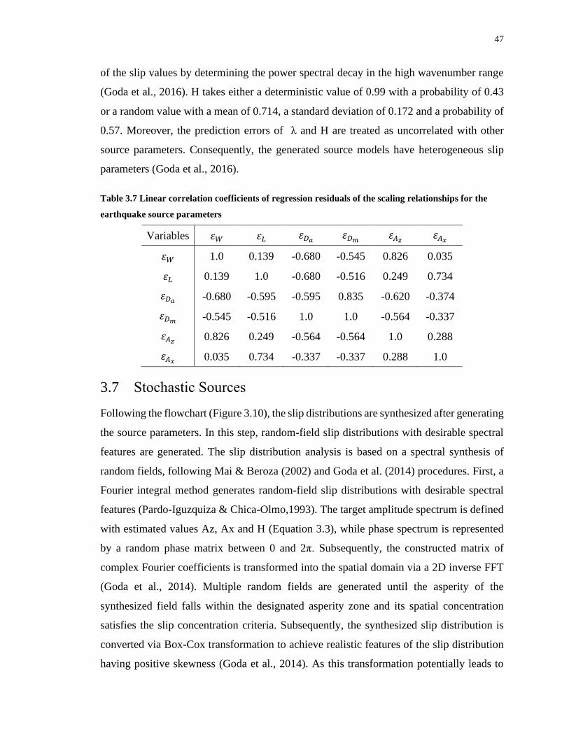
47
of the slip values by determining the power spectral decay in the high wavenumber range
(Goda et al., 2016). H takes either a deterministic value of 0.99 with a probability of 0.43
or a random value with a mean of 0.714, a standard deviation of 0.172 and a probability of
0.57. Moreover, the prediction errors of λ and H are treated as uncorrelated with other
source parameters. Consequently, the generated source models have heterogeneous slip
parameters (Goda et al., 2016).
Table 3.7 Linear correlation coefficients of regression residuals of the scaling relationships for the
earthquake source parameters
Variables 휀𝑊 휀𝐿 휀𝐷𝑎 휀𝐷𝑚 휀𝐴𝑧 휀𝐴𝑥
휀𝑊 1.0 0.139 -0.680 -0.545 0.826 0.035
휀𝐿 0.139 1.0 -0.680 -0.516 0.249 0.734
휀𝐷𝑎 -0.680 -0.595 -0.595 0.835 -0.620 -0.374
휀𝐷𝑚 -0.545 -0.516 1.0 1.0 -0.564 -0.337
휀𝐴𝑧 0.826 0.249 -0.564 -0.564 1.0 0.288
휀𝐴𝑥 0.035 0.734 -0.337 -0.337 0.288 1.0
3.7 Stochastic Sources
Following the flowchart (Figure 3.10), the slip distributions are synthesized after generating
the source parameters. In this step, random-field slip distributions with desirable spectral
features are generated. The slip distribution analysis is based on a spectral synthesis of
random fields, following Mai & Beroza (2002) and Goda et al. (2014) procedures. First, a
Fourier integral method generates random-field slip distributions with desirable spectral
features (Pardo-Iguzquiza & Chica-Olmo,1993). The target amplitude spectrum is defined
with estimated values Az, Ax and H (Equation 3.3), while phase spectrum is represented
by a random phase matrix between 0 and 2π. Subsequently, the constructed matrix of
complex Fourier coefficients is transformed into the spatial domain via a 2D inverse FFT
(Goda et al., 2014). Multiple random fields are generated until the asperity of the
synthesized field falls within the designated asperity zone and its spatial concentration
satisfies the slip concentration criteria. Subsequently, the synthesized slip distribution is
converted via Box-Cox transformation to achieve realistic features of the slip distribution
having positive skewness (Goda et al., 2014). As this transformation potentially leads to

48
very large slip, the transformed slip distributions are adjusted to achieve the target Da and
avoid large slip values of Dm. Moreover, the position of the synthesized fault plane is
determined (floated) randomly over the allowed fault plane, assuring the slip distributions
and locations of the source models are varied.
At this stage, the consistency of source parameters (W, L, and Da) is checked by comparing
the simulated seismic moment (𝑀𝑜 = 𝜇𝑊𝐿𝐷𝑎; 𝜇 = 4𝑥1010𝑁 𝑚⁄2) against the target
Figure 3.10 Flow chart of the stochastic method

49
moment magnitude of 7.7–7.9. If the simulated Mo does not meet the criteria, the source
parameters are generated until the simulated magnitude falls within the target magnitude.
Other criteria are implemented at this step to ensure that the synthesized slip distribution is
realistic with respect to the seismotectonic characteristics of the region. The first criterion
is that the Sa/S ratio of the simulated slip distribution falls within 0.194 and 0.286, where
Sa is the average fault area and S is the fault area. The second criterion is that 70% to 100%
of the simulated earthquake slip must concentrate in asperity regions. The third criterion is
that the difference between the observed and simulated vertical and horizontal deformations
must be less than 0.5. Lastly, additional adjustments of slip values are carried out by a taper
function to deeper segments of the fault plane. Finally, these steps are repeated until enough
acceptable stochastic source models are generated. An acceptable slip distribution is
required to have a Dm and similar slip concentration within the asperity zone.
3.8 Monte Carlo Tsunami Simulations
After generating a sufficient number of source models, tsunami simulations are performed
using a complete bathymetry and digital elevation models (DEM) dataset. The data are
presented as nested grid formulations, covering the entire western coast of Canada all the
way to California, USA. The steps for the tsunami simulations are presented in the
following sub-sections.
Bathymetry
Tsunami propagation and inundation modelling are highly sensitive to bathymetry and
elevation. The resolution of the bathymetry data can introduce significant uncertainty that
is difficult to quantify (Griffin et al., 2017). Therefore, accurate high-resolution DEM and
bathymetry datasets are required to generate realistic results (AECOM, 2013). For tsunami
modelling, the bathymetry data for Pacific coast is obtained from the General Bathymetric
Chart of the Oceans (GEBCO) dataset (2020) and is used for deep to shallow water regions.
The spatial resolution of the GEBCO dataset is 15 arc-seconds (≈450m). However, a high-
resolution onshore elevation is needed for an accurate simulation of tsunami run-up in the
shoaling regions near the coastline. Therefore, a 0.75-arc (∼20 m) Canadian Digital
Elevation Model (CDEM) is used for the onshore topography of the Canadian regions. The

50
CDEM original data are in orthometric height; the horizontal reference datum is the North
American Datum 1983 (NAD83), while the vertical reference datum is the Canadian
Geodetic Vertical Datum 1928 (CGVD28). The altimetric accuracy of the CDEM ranges
from 0 m to 10 m. Furthermore, 1-arc Shuttle Radar Topography Mission (STRM) DEM
is used for the regions in the USA. STRM data are in orthometric heights, the horizontal
datum is the WGS84, and the vertical datum is the Earth Gravitational Model 1996
(EGM96).
Potential errors can be introduced in the simulation depending on the dataset resolution (in
this case 450 m vs 30 m vs 20 m), the sources from which they are obtained, and the
collection date since the morphology and topology are likely to change over time (AECOM,
2013). Hence, the integration of bathymetry and elevation data are not trivial. In addition,
the effects of interpolation between the data sets can be significant at shallow depths near
the shoreline (Mori et al., 2017b.). Therefore, to minimize the errors in combining the
datasets, first, the three datasets are merged without interpolation, and the points are spaced
neither regularly nor uniformly. The duplicated values are eliminated during this step.
Secondly, at shallow depths, the values of the coarser dataset (GEBCO) are replaced by
those of the higher resolution datasets (CDEM for Canadian coasts and STRM for
American coasts) and the shoreline data are set as zero elevation data points. Finally, a
linear interpolation is performed for the combined datasets to provide a set of nested grids.
Linear interpolation is preferred over more complicated methods because it prevents the
over-interpolation of topographical features.
Nested Grid Formulations
The tsunami simulations are based on nested computational domains or nested grid
formulations. The nested grid system for the Haida Gwaii region uses four grid levels, i.e.
810 m-270 m-90 m-30 m (Figure 3.11). The grid formulations are nested by dividing the
large-scale coarse numerical grid by an integer of 3 (1/3 ratio rule) to avoid interference
problems in the tsunami simulations (Goda et al., 2016, Fine et al., 2018).

51
3.8.2.1 810 m Grid
The crudest level is 810 m region and covers the entire Haida Gwaii Islands and part of
Alaska, Oregon, Washington, and California. Six 270 m regions, thirteen 90 m regions, and
thirty-six 30m are defined within this grid. The extension of the 810 m grid must be
sufficient to resolve the feed-back effects from the smaller nested grids on the 810m grid.
The deformation due to fault ruptured is computed at the 810 m resolution using Okada
(1985) and Tanioka & Satake (1996) equations (Chapter 2). The 810 m grid is enough to
simulate deep-ocean tsunami waves since the effects from the topography are not as
relevant.
3.8.2.2 270 m Grid
The maximum wave amplitudes for the offshore observations (especially tide gauge
observations) are obtained in the six 270 m grids since a finer resolution is needed as the
observations are closer to the coast. The location and coverage of the grids are based on the
distances of the tide gauges. That is, all stations are within one of the 270 m grids. It is
important to note that grids with the same resolution must overlap with each other to ensure
that the solutions of the tsunami waves are propagated across different regions properly
(i.e. from deep ocean to shelf and into the coast) during the simulations, and no trapping of
shorter waves at the boundaries occur (Mori et al., 2017b, Fine et al., 2018).
3.8.2.3 90 m Grids and 30 m Grids
Thirteen 90 m grids are nested within the 270 m grid system. The 90 m grids are used to
propagate the tsunami wave from the 270 m grid resolution to 30 m resolution.
The low-elevation coastal areas are covered by thirty-six 30 m grids and have the highest
spatial resolutions of all grid formulations. This resolution is used for tsunami run-up
simulations as it can properly simulate the wave shoaling process along the coast.

52
Figure 3.11 Tsunami computational domains (810 m-270 m-90 m-30 m)

53
Tsunami Inundation Simulation
Tsunami simulations are performed for a set of acceptable source models. First, the initial
deformation is computed. The initial boundary conditions for tsunami simulations (initial
water elevation) are evaluated using Okada (1985) and Tanioka & Satake (1996)
(Equations 2.3-2.9). Afterward, the calculated surface elevation is smoothed using a 9-cell
by 9-cell moving average function to avoid steep initial water surface profiles. The
numerical computational code developed by Goto et al. (1997) is used for tsunami
propagation and inundation. The code uses a leap-frog staggered-grid finite-difference
scheme to solve the non-linear shallow-water equations (Equations 2.17-2.19) and
simulates the tsunami propagation from the source region to the offshore observation
locations and into coastal areas. The run-up is calculated by a moving boundary approach,
where a dry/wet condition of a computational cell is determined based on the total water
depth relative to the elevation. The bottom friction is evaluated using Manning’s formula
with a uniform Manning’s coefficient of 0.025 m-1/3/s. It is important to note that the
shallow-water formulations of tsunami propagations by Goto et al. (1997) cannot model
the dispersive tsunami waves for far-field tsunami wave profiles (Løvholt et al., 2012)
In the present study, two different simulation set-ups are used; the fault rupture is assumed
to occur instantaneously in both cases. The first simulation is to obtain the tsunami wave
amplitudes for offshore observation locations (tide gauges, DART buoys, and ONC’s
BPRs); the resolution of the 270 m grids is sufficient for this case. The numerical
calculation is performed for a duration of 6 hours with an integration time step of 1 second.
The integration time step is determined by satisfying the Courant-Friedrichs-Lewys
criterion. The second simulation case is to obtain the run-up levels. The resolution of the
30-m grids is used for the second simulation. The calculation is set for 2 h for the northern
sites and 1 hr for the southern sites, both with an integration time step of 0.1 seconds. No
tidal variation is considered for both simulation cases.
The steps mentioned above are repeated for all acceptable source models, and the tsunami
amplitudes and inundations at the observational locations are evaluated.

54
3.9 Results
Performance tests of the stochastic simulations are conducted by evaluating results from
the existing finite-fault models against observations (Section 3.4). The best matching model
is then compared against the stochastic models. The model by Gusman et al. (2016) agrees
well with the 2012 Haida Gwaii tsunami observations and thus is used to test the ability of
the stochastic source models to match the observations (further explanation in the following
section).
A brief discussion of the key features of the synthetic/stochastic earthquake slip models for
the 2012 Haida Gwaii earthquake is given. Then, the synthetic tsunami characteristics are
analyzed by comparing the tsunami simulation results with the existing observations of the
2012 event. Finally, to highlight the sensitivity of tsunami inundation to asperity areas, an
evaluation of the earthquake slip and fault geometry effects on coastal tsunami wave
heights along the Haida Gwaii region is carried out by comparing tsunami inundation
against run-up measurements (i.e. large slip areas).
Literature Finite-Fault Models
First, the tsunami simulations from the six literature source models are carried out for the
16 offshore observation stations (Figure 3.2). Then, the results and the observations are
compared against each other to find the best matching model (see Appendix A for the
complete results). Six observation sites (i.e. Queen Charlotte, Henslung Cove, Crescent
City, Cascadia Basin, Barkley Canyon, DART 46410; see Figure 3.2 for locations) are
chosen to illustrate the variation of the tsunami amplitudes based on their location along
the northwestern Pacific and to show the performance of each of the model to be able to
produce tsunami waves close to those of the 2012 event.
Special attention is given to the Queen Charlotte station (Figure 3.12) since the amplitudes
right after the rupture present negative values (a trough), which is interpreted as the
subsidence after the earthquake. The Gusman et al. (2016) model is the only model that
does not present this. Thus, a greater weight was given to this station in choosing which is
the best model to test the performance of the stochastic source models.

55
Next, the horizontal and vertical deformation of the models (Figure 3.13) are compared to
the observed deformations (See Appendix A for complete results). Some models (i.e. Wei,
2012, Shao & Ji, 2012, Hayes, 2013 [Fine et al., 2015], Hayes, 2017) have uplift on the
northern and southern parts of the island, which was not present in the observations. The
uplift presented in some models on the northern part of Haida Gwaii can be explained by
the source models’ length extending more than the actual rupture zone. In contrast, the
source models extending significantly beneath the island can explain the uplift on the
southern part. Whereas the models by Lay et al. (2013) and Gusman et al. (2016) present
Figure 3.12 Tsunami waveforms at Queen Charlotte, Henslung Cove, Crescent City, Cascadia Basin,
Barkley Canyon and DART 46410 stations and literature models

56
only subsidence, which means that the extension of the fault plane is limited to right beneath
the coastline.
The sum of square errors (sse) between the observations and the literature models is
calculated to find the best matching model. In addition, the error ratio between the
deformation observed and the simulated by the models is also considered. The model with
Figure 3.13 Horizontal and Vertical deformation vectors of the observations and source models from the
literature

57
the lowest sse (0.902) is the Gusman et al. (2016) model. Therefore, based on the tsunami
simulations, the deformation, and the Queen Charlotte station, the Gusman et al. (2016)
model was deemed the best matching model; thus, it was used to investigate the
performance of the stochastic source models to match both the observed deformations and
tsunami amplitudes.
Simulated Stochastic Source Models
A total of 1000 stochastic sources are generated for Mw 7.7 to 7.9 earthquakes, out of which
128 stochastic sources are chosen to perform Monte Carlo tsunami simulations. A summary
of the simulation parameters for the stochastic slip synthesis is presented in Table 3.8. The
simulation parameters are determined based on the six literature models, temperature
gradients, and aftershock sequences. All stochastic models consider uncertainty and have
diverse dimensions, slip distributions, slip heterogeneity, and locations. The slip
distributions used for Monte Carlo tsunami simulations are chosen based on the maximum
slip that fits the scenario Mw. The chosen slip distributions show how the slip values and
fault planes differ for similar Mw values. Consequently, the variations in slip distributions
can better account for the uncertainties of the source region. The models’ features are
controlled by the stochastic synthesis parameters and target slip, which significantly
influence the tsunami simulation results (Goda et al., 2014). Figure 3.14 shows the
variations in location, asperity sizes, and the maximum slip of some examples of the
stochastic source models. In general, models that closely match the observations are
constrained to the oceanward part of the fault and have major slip values within the asperity
region. The extension of the fault is also limited by the coastline and does not extend too
far beneath the islands, consistent with the coseismic subsidence deformation (Figure 3.14).
Table 3.8 Summary of stochastic earthquake slip simulation parameters
Model Parameter [Lowe, Upper]
Mw [7.7,7.9]
Slip ratio [0.7,1.0]
Ratio L/W [0.5,3.0]
Az to W range [0.35,0.5]
Ax to L range [0.2,0.5]

58
a) b)
c) d)
e) f)
Figure 3.14 (a-e) Five stochastic models (Mw 7.7-7.9), and (f) overall average slip models based on the
1000 stochastic sources

59
The vertical and horizontal deformations are constrained to an error ratio of 0.5 between
the target and simulated deformation values. Therefore, the source models have slip
distributions that produce deformations close to that of the 2012 event. Furthermore,
models that closely match the deformation also match the tsunami simulations (Figure
3.15).
Figure 3.15 Horizontal and vertical deformations of observations and stochastic models

60
Figure 3.14f shows the average source model generated by calculating the average slip of
every subfault of each of the 1000 stochastic source models. Most of the slip is concentrated
in the asperity region and is limited to the fault’s shallow side, consistent with the observed
aftershock sequences and thermal gradients of the zone. The overall Da is 1.96 m and falls
within the ranges used in past studies (Table 3.6).
Figure 3.16 Comparison of estimated source parameters for the stochastic models and six models
from literature against the corresponding global scaling relationships

61
The overall Dm of all the slip distributions is 9.97m, and it is larger than Dm of the past
models. It is important to note that the models used for the Monte Carlo tsunami simulations
are chosen based on whether the model’s Dm fell within the ranges of the global scaling
relationships for events of the same magnitude (Equation 3.7). The overall Mw is 7.76,
consistent with Mw considered in the six literature models (Mw 7.8). The overall length is
138 km, while the width is 53 km. Both dimension parameters are smaller than the ones
from the six literature models. However, they better fit the dimensions of the predicted fault
plane of 120–145 km length and 30 km width (Kao et al., 2015). The vertical and horizontal
deformations are constrained to an error ratio of 0.5 between the target and simulated
deformation values. Therefore, the slip models have slip distributions deformations close
to those of the 2012 event. Furthermore, models that present uplift are not accepted during
the stochastic source synthesis, further scrutinizing the stochastic models. Consequently,
models that closely match the deformation also match the tsunami simulations (Figure
3.15).
Figure 3.16 shows how the stochastic and literature models compare with the global scaling
relationships developed by Goda et al. (2016). The parameters for most stochastic source
models fall within the scaling equations’ prediction intervals (16th and 84th percentiles) in
comparison to the six models. The models by Hayes (2017) and Hayes (2013) (Fine et al.,
2015) have larger lengths than those expected from earthquakes of the same magnitude and
larger Az, which can contribute to the uplift present on the northern part of the islands. The
models’ width (W) is considerably smaller than those of the scaling relationships,
especially for the models of Shao & Ji (2012) and Lay et al. (2013). Thus, an increase in
slip values (Da and Dm) and a decrease in Ax values are expected. The increase in slip
concentrates tsunami waves (Momeni et al., 2020), which explains the higher amplitudes
produced by both Shao & Ji (2012) and Lay et al. (2013) models (Figure 3.12). On the other
hand, the larger W of Wei (2012) model results in lower Da and Dm, hence the overall
lower tsunami amplitudes.
Offshore Tsunami Result: Comparison with Observations
Due to time constraints from the 1000 stochastic source models, only 128 models are
chosen for Monte Carlo tsunami simulation based on their Dm. Thus, models that have Dm

62
within the expected Dm value for earthquakes of the same magnitudes are chosen over
those that have exceeding Dm. The tsunami wave characteristics of the 128 models are first
examined for offshore locations (i.e. tide gauges, DART stations, and ONC BPRs). In
general, the observations can be enclosed by the stochastic method. However, some models
perform better than others. Therefore, a comparison between the observations and each
model is preferred to find a set of the best matching models. The sum of squared errors
(sse; Equation 3.10) between the observed and simulated first wave amplitude are
calculated to identify the best matching source model for the 2012 event among the
stochastic slips (Table 3.9).
𝑠𝑠𝑒 = ∑(𝑂𝑏𝑠𝑒𝑟𝑣𝑎𝑡𝑖𝑜𝑛(𝑎𝑚𝑝𝑙𝑖𝑡𝑢𝑑𝑒) − 𝑠𝑖𝑚𝑢𝑙𝑎𝑡𝑖𝑜𝑛 (𝑎𝑚𝑝𝑙𝑖𝑡𝑢𝑑𝑒))2 (3.10)
Special attention is given to the Queen Charlotte station since some models start with
trough. Therefore, the sse of the first-hour wave amplitudes at the Queen Charlotte station
is also calculated and given greater weight. The tsunami waves that do not present this
trough at Queen Charlotte are the primary indicator for identifying the best matching source
model for the 2012 event. The sse values of all the stations for a given model are summed.
The stochastic source models are then ranked based on their calculated error metrics
(examples of best models are given in Figure 3.14). The deformation sse during the
stochastic source modelling is also considered in finding the best matching models.
Ultimately, two source models are chosen as the best models for offshore observations and
deformation. Model 168 has the lowest sse values (Table 3.9; Figure 3.14b); the model
matches the deformation best out of the models chosen for the tsunami simulation. In
contrast, Model 128 best matches the tsunami observations (Table 3.9; Figure 3.14e).
Figures 3.17 and 3.18 show the simulated time series of wave amplitudes at different
stations (i.e. Henslung Cove, Queen Charlotte, Winter Harbour, La Push, Port Orford,
Crescent City, Barkley Slope, Clayoquot Canyon, Cascadia Basin, DART 46419, DART
46410, DAR4611; see Figure 3.2 for location). The stations are chosen to illustrate the
variability in wave amplitudes with relation to the distance from major asperity zones. In
Figures 3.17 and 3.18, the individual tsunami wave profiles are shown in gray, the wave
profiles of the Gusman et al. (2016) model are shown in red, the best matching models in

63
green and orange, while the statistics (mean, 90th percentile, and 10th percentile) of the
tsunami simulation results are indicated in black to show major trends of the tsunami wave
profiles.
Table 3.9 Sum of square errors of the tsunami observations and deformation for the six literature
models and best stochastic source models
Models Deformation
Tsunami
Observations Total
sse sse
Lay et al. (2013) 1.602 1.221 2.824
Wei (2012) 7.024 1.096 8.119
Shao & Ji (2012) 12.268 1.13 13.397
Hayes (2013)
[Fine et al. 2015] 2.232 1.211 3.443
Gusman et al. (2016) 0.69 0.212 0.902
Hayes (2017) 2.331 1.225 3.556
Model 82 0.427 1.138 1.564
Model 120 0.533 1.121 1.654
Model 128 0.564 0.189 0.753
Model 168 0.303 0.208 0.511
Model 300 0.555 0.201 0.756
The results indicate that the mean wave amplitudes are similar to the observations.
Therefore, the simulations can closely match the observations. Although the average wave
profiles are not so large, some tsunami waves have larger amplitudes than the 90th percentile
wave. Nevertheless, the difference between the exceeding waves and the observations is
still small because the observation amplitudes are relatively small. As expected, stations
closer to the source (asperity areas) have relatively larger amplitudes (i.e. Winter Harbour
and Henslung Cove). Moreover, the high amplitudes might also be related to the stations’
location in the direct path of tsunami propagation. For the Queen Charlotte station (Figure
3.17), some models capture the deformation (subsidence) during the earthquake, interpreted
as the slip distributions extending too far beneath Haida Gwaii’s western coast (comparison

64
between Figure 3.14 and 3.19), explaining the negative values at the beginning of the
simulations.
Furthermore, the first wave amplitudes and the mean arrival times of the first wave are
close to the observations. However, the arrival times of the simulated first wave for the
station Ketchikan (Appendix A) are all early. Stations like DART 46410 and DART 46411
(Figure 3.19) have the most models with the smallest sse, while stations like Henslung
Cove and Winter Harbour (Figure 3.18) have the most stations with the largest sse. The
Figure 3.17 Comparison of time histories of tsunami wave for the 128 and 168 stochastic models
(mean, 90th percentile, and 90th percentile) and the Gusman et al. (2016) model with the
observations at different tide gauges

65
Model 128 better matches the observations at stations like DART 46410, Cascadia Basin,
Henslung Cove, Barkley Canyon, and Cascadia in comparison with the Gusman et al.
(2016) model, while at stations like Tofino, Port Orford, and Crescent City, the model
performs close or the same as the Gusman et al. (2016) model. On the other hand, Model
168 performs better at stations like Port Orford, Crescent City, and similar to Gusman et
al. (2016) model at stations like DART 46404, DART 46411, and DART 46419 (see
Appendix A for waveforms for Tofino).
Figure 3.18 Comparison of time histories of tsunami wave for the 128 and 168 stochastic models
(mean, 90th percentile, and 90th percentile) and the Gusman et al. (2016) model with the
observations at different ONC BPRs and DART buoys

66
Neither of the models present abnormal values for the Queen Charlotte station; thus, the
slip distributions do not extend too far beneath islands. The sse between the models and the
observation is 0.753 for Model 128 and 0.511 for Model 168, while the sse for the Gusman
model is 0.902.
Figure 3.20 Sites near the coast of Haida Gwaii
Figure 3.19 Figure 3.20 Stochastic source models for the 2012 Haida Gwaii earthquake with slip
distributions

67
The wave amplitudes for nearshore locations are calculated for the eight best models based
on the ability of the models to match the offshore observations. For the analysis, 20 sites
along the coast are chosen with depths of 30 m ± 10m (Figure 3.20). The sites are
distributed all along the western coast of Haida Gwaii, close to the run-up observational
sites. The results from the eight models are shown in gray, while the results from the
Gusman model are presented in green (Figures 3.21-3.22; see Appendix A for all sites).
The sites are chosen to explain further the variation of tsunami amplitudes due to the
location of major asperities. As expected, the results show that sites like Site 5, 7, and 20,
which are further away from the major asperity zone, have smaller wave amplitudes (i.e.
northern sites, Figure 3.21a).
The amplitudes become significant as the sites get closer to the epicentre and major asperity
regions. The largest amplitudes are recorded at sites like Sites 14, 15, and 16 (Figure 3.21b
and Figure 3.22). Generally, the sites to the north have smaller amplitudes compared to the
southern sites. Thus, the tsunami propagation path was mainly directed southward,
consistent with the large amplitudes recorded in places like Hawaii (Lay et al., 2013). In
addition, some models present earlier arrival times of the first wave’s amplitude than other
Figure 3.21 Time histories of tsunami waves for sites 5, 7,12, and 14

68
models, which is interpreted as the epicentre location of such models being too close to the
coast.
The maximum coastal tsunami wave heights along the coastline of Haida Gwaii are
generated by the eight stochastic models and the Gusman et al. (2016) model (Figure 3.23).
Note that the tsunami wave height that is discussed in this study is the height of water flow
above mean sea level. The maximum heights are calculated at 217 sites along the western
coastline of Haida Gwaii with approximately 10 m (±5m) depth. The results are shown in
gray in Figure 3.23 alongside the Gusman et al. (2016) model in green. The maximum
tsunami wave heights range from less than 1.0 m to 5.5 m. The maximum tsunami heights
for the southern part are higher than the northern part due to large slip areas on the southern
part (Figure 3.14), which are determined by the asperity region (Figure 3.9). The Gusman
et al. (2016) model has larger heights at coordinates 5.85x10⁶, while the stochastic models
have the largest heights at coordinates 5.82x10⁶. Both stochastic and Gusman et al. (2016)
models have similar amplitudes on the northern and southern limits.
Figure 3.22 Time histories of tsunami waves for locations 15,16, 18, and 20

69
Figure 3.24 shows the maximum wave amplitudes for the stochastic source models in
Figure 3.14 (See Appendix A for Model no. 300). Since no models had slip values on the
northern side of the QCF, the amplitudes for the models are relatively low in the northern
region, with wave heights less than 2 m. In comparison, zones directly in front of the rupture
have larger tsunami wave heights. Consequently, larger tsunami run-ups are expected in
the region. The run-up measurements in the zone differ significantly between sheltered sites
and exposed sites from storm waves (see Section 3.3.4). Exposed sites reported run-ups of
up to 7.37 m (Leonard & Bednarski, 2014, Table 3.4), whereas sites sheltered from storm
waves reported run-ups of 3.59 m, which agree more with the simulated maximum water
heights; this will be further discussed on the next section. Since most models had major
asperity areas on latitude 52.5º (Northing 5.83x10⁶ m), the largest heights for most of the
models are on those areas (see Figure 3.24). The largest run-up reported is also within this
zone (i.e. 12m at Davison Inlet, Leonard & Bednarski, 2014); however, it is important to
note that the site was exposed to storm waves, which could result in such a high value.
Figure 3.23 a) Maximum coastal tsunami wave heights generated by the eight stochastic models and
the Gusman et al. (2016) model, and b) sites along the shoreline of Haida Gwaii

70
Figure 3.24 Maximum wave height for the Haida Gwaii region

71
Onshore Tsunami Results: Comparison with Run-up Observations
To study the variability of tsunami inundation with changing asperity zones, the tsunami
inundation for different bays and inlets, where run-up observations were collected (see
Section 3.3.4), is calculated for the eight best matching models from the previous section.
Tsunami inundation in coastal areas is affected by three main factors: the source (large slip)
characteristics, the bathymetry features of the coastal area, and the shape of the bay (Mori
et al., 2017b, Momeni et al., 2020). The Haida Gwaii topography consists of cliffs and
fjords, which could amplify the tsunami inundation within the bays and inlets. The tsunami
inundation is calculated from different points along the bays and inlets. The inundation
average for the bay or inlet is compared against the run-up reported by the field surveys.
Overall, the highest inundations are observed on sites near the epicentre, where the highest
slip values are concentrated, with inundation heights of up to 4.56 m (i.e. Kwoon Cove and
Pocket Inlet, see Figure 3.6 for the locations). On the other hand, sites north of the Haida
Gwaii region, which have small or no areas of concentrated slip, have lower inundations
than the southern sites. The differences correlate to the water heights from Figure 3.24.
The run-up observation sites are divided into sites sheltered from storm waves and sites
exposed to storm waves (Leonard & Bednarski, 2014). The highest run-up heights were
generally at sites exposed to storm waves (Table 3.4). The comparison of the simulation
results against the observations shows a significant difference, particularly at sites exposed
to storm waves. Overall, the simulation results are lower than those reported by Leonard
and Bednarski (2010; Table 3.10), with differences ranging from 3 m to 7 m. It is important
to note that there is some uncertainty in the run-up observations, especially at sites exposed
to storm waves, because the field surveys were conducted several weeks after the 2012
event, right after a major storm hit the region. Thus, making the differentiation between
tsunami and storm effects difficult, especially for exposed sites. The six models from the
literature also presented lower values at the sites exposed to storms, with Lay et al. (2013)
model having the highest inundation profiles (see Appendix A).

72
Table 3.10 Run-up values for nine stochastic sources along the Haida Gwaii region
At sites sheltered from storm waves, the simulation results present closer run-up heights to
those of the observations, with differences between 1 m and 3 m. Out of the eight models
used for calculating run-up, Model 82 (Figure 3.14a) yields the best results and has the
smallest differences between the observed and simulated run-up. The spatial variability of
the maximum tsunami inundation height along the coastal line in the Haida Gwaii region
is shown in Figure 3.24 for Model 82. It is observed that the inundation heights are
governed by slip concentration in the asperity areas by comparing the inundation heights
and wave amplitudes. Thus, models with higher slip values generated higher inundation
and wave profiles. It is also important to note that some range of error in the DEM data can
also affect the tsunami simulations, especially close to the coast.
Sites Model
82
Model
120
Model
128
Model
168
Model
185
Model
300
Model
685
Model
828
Otard Bay 0.98 0.82 0.89 0.97 0.96 0.95 0.97 0.88
Seal Inlet 0.39 0.31 0.32 0.34 0.42 0.40 0.48 0.27
Gudal Bay 0.95 0.64 0.96 0.87 1.12 1.09 1.17 0.65
Saunders
Island 0.76 0.66 0.66 0.82 0.77 0.56 0.77 0.46
Davidson
Inlet 3.25 2.10 2.60 2.53 1.78 1.96 1.78 1.97
Sunday
Inlet 4.06 2.77 3.21 3.02 3.13 2.88 3.13 2.98
Kwoon
Cove 4.38 3.30 3.83 3.69 3.10 2.98 3.10 3.69
Inlet 4.56 3.24 3.91 3.84 3.23 3.05 3.23 3.83
Mike Inlet 4.71 3.12 3.40 3.98 3.69 3.58 3.69 4.26
Puffin
Cove 3.92 3.35 2.78 3.41 3.22 3.74 3.22 3.77
Goski Bay 1.72 1.80 1.46 1.50 1.47 2.03 1.47 1.87
Staki Bay 2.06 0.76 1.09 1.24 1.24 1.56 1.24 1.38
Louscoone
Inlet 0.99 0.46 0.55 0.58 0.73 0.73 0.73 0.53
Ta'dasl 2.00 1.26 0.54 1.50 1.51 1.52 1.51 0.88
Gilbert Bay 2.00 1.26 0.54 1.50 1.51 1.52 1.51 0.88

73
3.10 Conclusions
The stochastic tsunami simulations for Mw 7.7-7.8 scenario were calculated for the Haida
Gwaii region. The uncertainties were considered for the source geometry and slip
distributions during the stochastic source models synthesis. The variability of source
parameters and fault geometries for the region based on global scaling relationships
highlighted the sensitivity of the tsunami waves and tsunami inundation to the areas with a
high slip concentration. Therefore, the more concentration of slip in the areas of interest
will result in higher amplitudes. Moreover, the usage of multiple observations to constrain
such parameters validates the results.
Furthermore, a set of models that match the observations can better represent the
uncertainty of the events and help better understand the tsunami hazard of the region. The
inclusion of uncertainty and variability and the usage of multiple observations are important
improvements to the approaches used by previous studies. This is further shown by lower
squared errors (i.e. 0.511 and 0.753 of Model 168 and Model 128 respectively; Table 3.9)
than the previous source models of the region (i.e. lowest of 0.902 from Gusman et al.
model; Table 3.9). Thus, the comparison against the Gusman et al. (2016) model and the
Monte Carlo tsunami simulations shows that the stochastic source models can produce
realistic tsunami results similar to those of the 2012 Haida Gwaii tsunami. However, the
run-up values for the stochastic source models were lower than those reported by the post-
tsunami field surveys. This discrepancy between run-up values could be the result of severe
storms overprinting the tsunami observations. This overprinting can be shown by the larger
differences between the simulated run-up and the run-up on sites exposed to storm waves
and lower differences at sheltered sites. Nevertheless, the stochastic method and Monte
Carlo tsunami simulations can provide important information about possible tsunami
outcomes for the Haida Gwaii region, thus quantifying uncertainties in the prediction of
tsunami hazards.

74
Chapter 4
4 Future Tsunami Scenarios for the Haida Gwaii Region
Historically, the Haida Gwaii region experienced Mw 8 (i.e. 1949 earthquake) strike-slip
earthquakes on the north side of the fault, while an Mw 7.8 (i.e. 2012 earthquake) thrust
earthquake occurred on the southern part of the fault. Although the 1949 earthquake was a
pure strike-slip event, it generated a small tsunami. The lack of tsunami observations might
be due to the fault’s strike-slip mechanism or the lack of settlements and observation
stations along the coast of Haida Gwaii (Cassidy et al., 2014). Apart from those events,
another event (i.e. 2001 Mw 6.1 earthquake) caused a tsunami in the region. The 2001
earthquake generated a larger than expected tsunami. The larger tsunami waves might have
resulted from the 30 km length of the effective seismic source, which is larger than the 15
km length from the actual seismic source expected for the magnitude and the aftershock
sequences (Rabinovich et al., 2008). An explanation for this more extensive effective
seismic source is that the rupture extended into the soft sediments of the Queen Charlotte
Terrace (QCT), amplifying the displacement of the earthquake (Rabinovich et al., 2008).
The QCT is an irregular terrace extending from the south end of the Haida Gwaii islands
to their north end and has a depth of 1000m (Hyndman, 2015; Figure 4.1). Furthermore,
the QCT runs parallel to the margin between the Pacific-North American Plates. As it
moves northwest along the margin, the convergence component decreases as it reaches the
eastward part of the Queen Charlotte Fault (QCF) on the western side of Graham Island.
Thus, on the southwestern side, the underthrusting and convergence follow pre-existing
fractures and thrusts at the base of the terrace.
The 2012 earthquake only ruptured half of the available fault area (Allen et al., 2015).
Moreover, Kao et al. (2015) suggested that most of the elastic strain along the QCF was
not released during the 2012 earthquake. This is suggested based on the 2012 Haida Gwaii
earthquake’s aftershocks distribution extending no further than the seismic gap, and none
were larger than Mw 4.8. Additionally, there is a possibility of the slip extending toward
the northern part of the fault, given the locations of the relocated aftershock distributions,
which show that the 2012 source region correlates with the southern part of the 1949 event.

75
Therefore, this information supports the likelihood of a major strike-slip earthquake on the
northern part of the region that can extend to the southern part and release the thrust
component of the QCF in the future, causing a larger tsunamigenic event than the 2012 Mw
7.8 earthquake. Consequently, the 2012 Haida Gwaii event provides important information
about the region's seismicity, which allows studying possible future events and creating
proper risk mitigation strategies for the region.
The chapter is organized as follows. First, the methodology for the stochastic source
modelling and the Monte Carlo tsunami simulation for future larger events is explained.
The present scenario considers events with Mw ranging from 7.9 to 8.1. Furthermore, a
Figure 4.1 The Oshawa rise, Queen Charlotte Trough (trench), Queen Charlotte terrace
(accretionary sedimentary prism), and Queen Charlotte ranges (uplifted edge of continent). The
dashed lines show the model extent of the underthrust plate for 2.5 and 6 million years, that is,
for the triple junction at Brooks Peninsula (from 6 Ma) and at the Wilson Knolls (from 2.5 Ma).
It is assumed that there has been no significant crustal shortening in these estimates. (Hyndman,
2015)

76
broader asperity zone is considered to produce larger magnitudes. Historical events, such
as the M8.1 event, motivate applying the stochastic method (if slip extends toward the
northern part of the fault) and Monte Carlo tsunami simulation to a slightly larger event
and without strict constraints based on the observations from 2012. Finally, the results of
the tsunami analysis of future larger events are explained in detail for offshore and onshore
observations.
4.1 Procedure
Following the same methodology from Chapter 3, the earthquake scenario is first defined
by specifying the target Mw, fault model, and asperity zone (Figure 4.2). An Mw range of
7.9 to 8.1 is considered based on the existence of the QCT and oblique movement of the
fault, which can release the thrust component in the region, thus, rupturing both the strike-
slip mechanism on the north and thrust mechanism on the south of the fault. Then, the
synthetic fault model is developed based on the geometry of the fault plane (strike and dip).
Figure 4.2 Map showing the synthetic fault plane (black) and the asperity zone
(red) defined for this study

77
The fault model from Chapter 3 (Figure 3.8) is also used for this case since it covers the
entire length of the QCF. The width is based on the QCT (Hyndman, 2015); however, it is
larger to allow different geometry during the stochastic synthesis. The synthetic fault covers
an area spanning 315 km along strike and 95 km along dip, with a constant strike of 325°
and dip angle of 20°. The asperity region is a sub-region within the fault that has a
significant amount of earthquake slip. In this scenario, an asperity zone different from that
of the 2012 Haida Gwaii earthquake is considered. The asperity is larger than that of the
2012 event and is based on the extension of the QCT (Hyndman, 2015) and the thermal
constraints of the fault (Wang et al., 2015; Figure 4.2). The present scenario’s parameters
reflect the hypothesis that all parts of the QCT can simultaneously rupture.
Secondly, earthquake source parameters (width W, length L, slip average Da, slip
maximum Dm, Box-Cox parameter λ, correlation length along strike Ax, correlation length
along dip Az, and Hurst number H) are calculated using scaling relationships by Goda et
al. (2016; Equations 3.4-3.9). The uncertainty and the correlation associated with regression
models should be taken into account in sampling the values of the source parameters. Thus,
the sampling regression prediction errors of the scaling relationships avoid unrealistic
combinations of source parameters and are sampled from the multivariate normal
distribution function in a logarithmic space (Table 3.7).
Third, a Fourier integral method generates a random slip field based on the generated slip
distribution parameters (Pardo-Iguzquiza & Chica-Olmo, 1993). Then, the synthesized slip
distribution is converted via Box-Cox transformation to achieve a slip distribution with
realistic positive skewness (Goda et al., 2014). The resulting slip distribution is then
adjusted to the target Da and Dm to avoid undesirable slip values. Subsequently, the
location of the fault plane is determined randomly within the synthetic fault plane, and the
simulated values are constrained by comparing the target and simulated moment magnitude
(𝑀𝑜 = 𝜇𝑊𝐿𝐷𝑎 , where μ is the rock rigidity and is set to 40 GPa; Gusman et al., 2016).
Only models that fit the set criteria are accepted; thus, the steps are repeated until a model
that falls within the criteria is generated. Finally, further constraints are applied to ensure a
realistic synthesized slip distribution (Table 4.1). The first one is that the ratio between the
average fault area and the fault area (Sa/S) falls within a range of 0.194 to 0.286. The second

78
constraint is that the ratios between the correlation lengths (Az or Ax) and the geometry
parameters (W, or L) are in the ranges of 35 % to 50% and 20% to 60%, respectively, based
on the extension of the QCT, and thermal constraints (i.e. 1949 M. 8.1 earthquake). The
final constraint is that 70 % to 100% of the simulated earthquake slip must concentrate on
asperity regions.
Table 4.1 Summary of stochastic earthquake slip simulation parameters
Model Parameter [Lowe, Upper]
Mw [7.9 8.1]
Slip ratio [0.7,1.0]
Ratio L/W [0.5,6.0]
Az to W range [0.35,0.5]
Ax to L range [0.2,0.6]
Fourth, the Monte Carlo tsunami simulation is carried out. The initial water surface
elevation is calculated using Okada (1985) and Tanioka & Satake (1996) (Section 2.3). The
tsunami wave propagation is calculated by solving the non-linear shallow-water equations
with run-up (Equations 2.17-2.19; Goto et al., 1997). A bathymetry 2020 dataset is obtained
from the Geometry Bathymetric Chart of the Oceans (GEBCO) for deep to shallow water
regions, while digital elevation models (DEM) are obtained for the onshore topography.
The Canadian Digital Elevation Model (CDEM) is used for the Canadian coasts, whereas
the Shuttle Radar Topography Mission (STRM) DEM is used for the American coasts.
Moreover, the bottom friction is evaluated using Manning’s formula, and the fault rupture
is assumed to occur instantaneously. Computational domains are used for the tsunami
propagation simulations and follow a 1/3 ratio (i.e. 810 m, 270 m, 90 m, 30 m; see Section
3.8.2). The grid nesting from coarse to fine resolution is done so the large to small-scale
tsunami waves can be considered based on changes in water depth. For the present scenario,
the finer resolution used is 270m, which is coarse to evaluate the run-up in coastal areas.
Therefore, an extensive inundation calculation is excluded in this study, and error range
should be considered for the nearshore results. The vertical displacement of water due to
earthquake rupture (Okada, 1985) and the horizontal effects of steep slopes on the vertical
displacement of water (Tanioka &Satake, 1996) are computed at the 810-m resolution.
Then, the numerical tsunami calculation is performed for 6 hours with an integration time
step of 1 s to satisfy the Courant-Friedrichs-Lewis condition. Finally, the above procedure

79
is repeated until sufficient source models are generated, and the tsunami simulations are
evaluated.
4.2 Results
Simulated Stochastic Source Models
The magnitude range of Mw 7.9 to 8.1 was considered for the stochastic source models. A
total of 326 stochastic source models were generated with a diverse set of source parameters
and slip characteristics to account for uncertainties and variabilities. Overall, the models
are consistent with global scaling relationships, as presented in Figure 4.3, and mostly fall
within the prediction intervals (16th and 84th percentiles). However, some models had
larger L and Az than earthquakes for similar magnitudes. These larger values are expected
since the fault is rupturing entirely.
Figure 4.4 shows stochastic source examples and the variability of the fault’s geometry and
asperity regions. This highlights the ability of the stochastic source modelling method to
generate variable source models for a given scenario. It can be observed that both the plane
size and slip values increase with Mw, and the location and size of the asperity areas also
change. These features have a significant influence on tsunami simulation results. They are
controlled by the target slip, Mw, and stochastic synthesis parameters (Goda et al., 2016,
Mori et al., 2017b, Momeni et al., 2020). Moreover, the hypocentre is likely to be located
near the fault’s shallow side and around subfaults with relatively large slip. Thus, the
hypocentre is more likely to be in the asperity areas. In this case, since the asperity zone
was set up to cover the entire length of the fault plane, the slip concertation varies more
widely across models, which differs from the more constrained 2012 scenario. This
variability allows accounting for different possibilities of slip concentration in future
events. The overall Da is 1.67 m which falls within the ranges of the global scaling
relationships. The overall Dm for all 326 slip distributions is 8.97 m and is similar to the
scaling relationships. The overall Mw is 7.98 and represents possible larger events in the
region. The average L is 241 km, whereas the average W is 82 km. The L of some models
is larger than the global scaling relationships, whereas the W of other models is smaller
than expected. For the present scenario, no slip distribution was constrained by deformation

80
observations, as was done for the 2012 Haida Gwaii event. The present stochastic source
models can then generate realistic earthquake scenarios and the effects of the corresponding
tsunamis. Figure 4.4f shows the overall average slip model, generated by calculating the
mean slip of subfaults of the 326 stochastic sources with the large slip areas concentrated
to the shallow part of the fault plane. For this scenario, the best model is not chosen, but
instead, the results and 2012 tsunami observations are compared.
Figure 4.3 Comparison of 326 stochastic source parameters (green dots) with the corresponding
scaling relationships.

81
a) b)
c) d)
Figure 4.4 (a-e) Five stochastic models (Mw 7.9-8.1), and (f) overall average slip models based on the
326 stochastic sources
e) f)

82
Far-Field Results
A total of 326 stochastic source models are used for the Monte Carlo tsunami simulations.
The tsunami wave characteristics of the stochastic models are examined for the far-field
locations. The tsunami waves amplitudes are simulated for the far-field results on tide
gauges, DART stations, and ONC BPRs that recorded the 2012 tsunami. The amplitudes
of the larger tsunami are compared against the observations of the 2012 event to evaluate
the difference between tsunami wave amplitudes of the observations (Mw 7.8) and larger
Mw events (Mw 7.9-8.1). In Figures 4.5 and 4.6, the individual tsunami wave profiles for
different stations (i.e. Henslung Cove, Queen Charlotte, Winter Harbour, La Push, Port
Orford, Crescent City, Barkley Slope, Clayoquot Canyon, Cascadia Basin, DART 46419,
DART 46410, and DART 46411; see Figure 3.2 for locations) are shown in gray, the
statistics are shown in black (mean, 10th, and 90th percentiles), while and the observations
of the 2012 Haida Gwaii tsunami are shown as a thick black line (see Appendix B for
tsunami wave profiles of all the stations).
Stations on the north (i.e. Henslung Cove, DART 46410, and Ketchikan), middle (Winter
Harbour, Queen Charlotte, and Cascadia Basin, Barkley Slope, Clayoquot Canyon, and
DART 46419), and south (i.e. La Push, Port Orford, Crescent City, and DART 46411) are
chosen to demonstrate the variability of tsunami wave amplitude based on the proximity to
the asperity regions and to show the effects of regional slip patterns on tsunami profiles.
As expected, the results show that the wave amplitudes are larger than those observed
during the 2012 Haida Gwaii tsunami. The tsunami profiles at these different locations are
variable. The average of the wave profiles is close to the observations of the 2012 events
and does not vary significantly. However, some tsunami waves are several times greater
than the average tsunami amplitudes and observations and exceed the 90th percentile.
Stations like Cascadia Basin and DART 46411 (Figure 4.6) have wave amplitudes almost
twice as large as the 90th percentile. There is more variability in both tsunami amplitudes
and time arrivals depending on the location of the asperity areas since the asperity zone for
this scenario extended along the entire fault’s length. Deep-ocean observations present
higher values than those recorded for the smaller 2012 event. For stations like Cascadia

83
Basin, DART 46410, and DART 46411, the tsunami waves have amplitudes that are three
times as large as the observations.
Tsunami wave profiles are affected by proximity to the asperity areas. Stations closer to the
rupture zone have the highest amplitudes, like Queen Charlotte, Winter Harbour and
Henslung Cove (Figure 4.4). Some simulations start with a trough at northern stations like
Henslung Cove and Ketchikan (see Appendix B). The reason might be that the extension
of the fault rupture lengths extended too far north. Slip distributions like Model 228 (Figure
4.4d) do not present this trough at the Ketchikan station, whereas for the Henslung Cove
Figure 4.5 Comparison of time histories of tsunami wave for the 326 stochastic models (mean, 90th,
and 10th percentile) and observations

84
station, it only presents a slight trough. Models, such as Model 123 (Figure 4.4c), presented
both troughs at such stations. Therefore, the results can help limit the extent of the fault
length on the northern part.
The Queen Charlotte station (Figure 4.5) presents a trough at the beginning of the tsunami
waveforms, just like stations Henslung Cove and Ketchikan. However, for the station, the
slip distributions of some stochastic models extend too far beneath the islands. For example,
although the length of Model 123 (Figure 4.4c) does not extend to the south, the width
covers most of the island, and some subfaults with significant slip are beneath the islands.
Figure 4.6 Comparison of time histories of tsunami wave for the 326 stochastic models (mean, 90th,
and 10th percentile) and observations
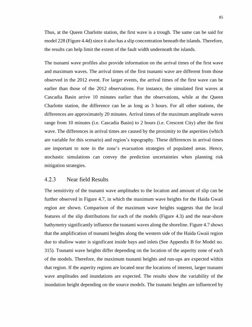
85
Thus, at the Queen Charlotte station, the first wave is a trough. The same can be said for
model 228 (Figure 4.4d) since it also has a slip concentration beneath the islands. Therefore,
the results can help limit the extent of the fault width underneath the islands.
The tsunami wave profiles also provide information on the arrival times of the first wave
and maximum waves. The arrival times of the first tsunami wave are different from those
observed in the 2012 event. For larger events, the arrival times of the first wave can be
earlier than those of the 2012 observations. For instance, the simulated first waves at
Cascadia Basin arrive 10 minutes earlier than the observations, while at the Queen
Charlotte station, the difference can be as long as 3 hours. For all other stations, the
differences are approximately 20 minutes. Arrival times of the maximum amplitude waves
range from 10 minutes (i.e. Cascadia Basin) to 2 hours (i.e. Crescent City) after the first
wave. The differences in arrival times are caused by the proximity to the asperities (which
are variable for this scenario) and region’s topography. These differences in arrival times
are important to note in the zone’s evacuation strategies of populated areas. Hence,
stochastic simulations can convey the prediction uncertainties when planning risk
mitigation strategies.
Near field Results
The sensitivity of the tsunami wave amplitudes to the location and amount of slip can be
further observed in Figure 4.7, in which the maximum wave heights for the Haida Gwaii
region are shown. Comparison of the maximum wave heights suggests that the local
features of the slip distributions for each of the models (Figure 4.3) and the near-shore
bathymetry significantly influence the tsunami waves along the shoreline. Figure 4.7 shows
that the amplification of tsunami heights along the western side of the Haida Gwaii region
due to shallow water is significant inside bays and inlets (See Appendix B for Model no.
315). Tsunami wave heights differ depending on the location of the asperity zone of each
of the models. Therefore, the maximum tsunami heights and run-ups are expected within
that region. If the asperity regions are located near the locations of interest, larger tsunami
wave amplitudes and inundations are expected. The results show the variability of the
inundation height depending on the source models. The tsunami heights are influenced by

86
the source, tsunami path and topography. Hence, the tsunami wave heights are spatially
variable.
Figure 4.7 Maximum wave height for the Haida Gwaii region

87
4.3 Conclusions
Stochastic earthquake source models in Monte Carlo tsunami simulations are useful in
including the uncertainties of tsunami simulations and show the variability and sensitivity
of tsunami wave amplitudes depending on slip values and asperity regions. The stochastic
source models for possible Mw 8 earthquakes in the Haida Gwaii region took into account
uncertainties of the location and source parameters of the fault. This is shown in the
variability of the slip distributions of the source parameters used in Monte Carlo tsunami
simulations and the maximum wave heights and the time series at different stations. The
results highlighted the method's usefulness to explore different possible tsunami amplitudes
and inundations for a given scenario, which can help predict possible tsunami hazards to
coastal communities and make informed decisions in risk mitigation strategies. The
tsunami analysis of future larger events is challenging because of the uncertainties in how
the next scenario will happen and the various assumptions made. For the given scenario,
various improvements can be made, like finer computational domains to assess better the
inundation of coastal areas, and the tsunami simulation of more stochastic source models.
The following points can further improve some of the limitations of the present study:
1. The use of higher-resolution bathymetry and DEM datasets to reduce errors in the
tsunami simulation.
2. The use of geological evidence of past events in the region to better predicts the
fault's mechanism.
Finally, the results of the tsunami simulations can be used in future work to constrain
possible parameters like the possible slip concentration and validate the models based on
the inundation of areas of interest for larger events in the zone, like the ones from the
Cascadia Subduction Zone.

88
Chapter 5
5 Conclusions
The thesis objectives were to develop stochastic slip models for Haida Gwaii earthquakes
and analyze the tsunami hazard along the western North Pacific coastline due to such events
in terms of tsunami wave profiles at observation stations and maximum tsunami wave
heights along the Haida Gwaii using Monte Carlo tsunami simulations. An extensive
tsunami simulation was performed by developing many stochastic source models for both
the 2012 Haida Gwaii event (i.e. 128 stochastic source models) and future larger events
(i.e. 326 stochastic source models) with magnitude ranges of 7.7-7.9 and 7.9-8.1, for each
earthquake scenario, respectively.
For the 2012 Haida Gwaii scenario, the earthquake source regions from six inversion
models from the literature were first evaluated and compared against global scaling
relationships (Goda et al., 2016). Then a synthetic fault model was defined for stochastic
source synthesis. The same synthetic fault plane was used for both Mw scenarios. The
asperity zone was then defined. For the 2012 scenario, the asperity zone was based on the
region's aftershock sequence and thermal constraints. In contrast, the asperity zone for
larger events was based on the extension of Queen Charlotte Terrance, significant slip areas
from the 1949 Mw 8.1 earthquake, and the oblique seismic movement that might release
the fault's thrust component. Deformation observations were used as a constraint during the
synthesis of the stochastic sources for the 2012 scenario, while no such constraint was used
for the larger future events. Uncertainty and variability of earthquake source parameters
were accounted for when producing the stochastic source models.
Both tsunami simulation results were compared against the 2012 observations recorded on
Canadian and American tide gauges, Ocean Network Canada bottom pressure sensors, and
DART buoys. Furthermore, the simulated tsunami wave profiles from the 2012 scenario
were compared against the Gusman et al. (2016) model to test the performance of the
simulations. The tsunami wave amplitudes were further evaluated using the tsunami wave
profiles at 20 sites at 30 m depth along the coastline. The maximum tsunami wave height
at 217 sites at 10 m depth. Moreover, the run-up was calculated for the best eight models

89
and compared to the run-up reported by field surveys (Leonard and Bednarski, 2014). The
tsunami wave profiles produced from the stochastic source models for the 2012 scenario
are in good agreement with those of the 2012 Haida Gwaii event and are comparable to
those of the Gusman et al. (2016) model. The results from the future events show larger
amplitudes than those of the 2012 events and earlier arrival times of the first wave. The
evaluation of tsunami run-up was not possible for the larger events since the grid system
used during tsunami simulations was too coarse.
The results show that the stochastic method can help constrain the source characteristics of
a given event and how different geometries and parameters can produce similar results.
Furthermore, the method helps to have a broader picture of the possible future scenarios
and provides important information that can be used for risk mitigation planning as it helps
constrain parameters that can be used for forecasting future events.
5.1 Limitations
The results show the importance of incorporating uncertainty when modelling earthquake
source models since the location and amount of slip greatly affects the tsunami heights and
concentration. Furthermore, the stochastic method allows constraining the source
parameters for possible future events useful in tsunami forecasting and risk mitigation
planning. However, it is important to note the limitations of the present study. One
limitation is the distance range to simulate tsunami propagation. The present method and
computational code used can only estimate tsunami propagation to relatively close
distances (couple of thousand kilometres) from the source, since larger distances would
need the use of spherical coordinates and take into account the curvature of the Earth’s
surface.
Another limitation depending on the type of analysis, is that the method is computationally
demanding. This limitation is notable in the present study since many simulations for both
earthquake scenarios (offshore and onshore) would have been preferred. Moreover, a more
accurate Digital Elevation Model (DEM) is needed to reduce the run-up simulation errors
further because the simulations need to take into account the topography of the ocean
bottom.

90
5.2 Future Work
In future studies, tsunami simulations for the finer grid system (i.e. 30m) should be run
more extensively to further analyze the run-up extension in the Haida Gwaii region. In
addition, more simulations for offshore and nearshore locations are needed to constrain
better source parameters. This is especially true for future events since the coarse grid used
in the present simulations is too large to calculate run-up locations.
Furthermore, an extensive sensitivity analysis needs to be carried out for the source region
parameters by changing some parameters and evaluating the effects of the changes in the
tsunami simulations. The occurrence probability might also be included to extend this work
to a complete probabilistic tsunami hazard analysis. A more detailed study can be done
with more simulations for Haida Gwaii events for special areas of interest like cities of
towns, based on proximity to areas with likely slip clustering. Furthermore, Cascadia
Subduction Zone simulations events can use the inundation patterns of the larger events’
results to constraint the possible parameters for future subduction events.

91
References
AECOM. (2013). Modeling of potential tsunami inundation limits and run-up. report for
the capital region district. (Project Number: 60242933).
Allen, T.I., Adams, J., Halchuk, S., & Rogers, G.C. (2015). 5th Generation Seismic Hazard
Model for North-Western Canada. The 11th Canadian Conference on Earthquake
Engineering. (Paper Number: 937982)
An, C., Liu, H., Ren Zhiyuan, Y., & Yuan. (2018). Prediction of tsunami waves by uniform
slip models. Journal of Geophysical Research: Oceans,123, 8366–8382.
https://doi.org/10.1029/2018JC014363
Atwater, B.F., Musumi-Rokkaku, S., Satake, K., Tsuji, Y., Ueda, K., & Yamaguchi, D.K.
(2015), The orphan tsunami of 1700—Japanese clues to a parent earthquake in
North America, 2nd ed.: Seattle, University of Washington Press, U.S. Geological
Survey Professional Paper 1707, 135 p
Barth, S., Geertsema, M., Bevington, A. R., Bird, A. L., Clague, J. J., Millard, T.,
Bobrowsky, P. T., Hasler, A., & Liu, H. (2020). Landslide response to the 27
October 2012 earthquake (MW 7.8), southern Haida Gwaii, British Columbia,
Canada. Landslides, 17(3), 517–526. https://doi.org/10.1007/s10346-019-01292-7
Bernard, E., & Titov, V. (2015). Evolution of tsunami warning systems and products.
Philosophical Transactions of the Royal Society A: Mathematical, Physical and
Engineering Sciences, 373, 20140371. https://doi.org/10.1098/rsta.2014.0371
Bird, A. L., & Lamontagne, M. (2015). Impacts of the October 2012 magnitude 7.8
earthquake near Haida Gwaii, Canada. Bulletin of the Seismological Society of
America, 105, 1178–1192. https://doi.org/10.1785/0120140167
Blaser, L., Krüger, F., Ohrnberger, M., & Scherbaum, F. (2010). Scaling relations of
earthquake source parameter estimates with special focus on subduction
environment. Bulletin of the Seismological Society of America, 100, 2914–2926.
https ://doi.org/10.1785/0120100111

92
Brothers, D. S., Miller, N. C., Barrie, J. V., Haeussler, P. J., Greene, H. G., Andrews, O.,
BrianD., Zielke, Watt, J., & Dartnell, P. (2020). Plate boundary localization, slip-
rates and rupture segmentation of the queen charlotte fault based on submarine
tectonic geomorphology. Earth and Planetary Science Letters. 530, 115882.
https://doi.org/10.1016/j.epsl.2019.115882
Cassidy, J. F., Rogers, G. C., & Hyndman, R. D. (2014). An overview of the 28 October
2012mw 7.7 earthquake in Haida Gwaii, Canada: A tsunamigenic thrust event along
a predominantly strike-slip margin. Pure and Applied Geophysics. 171(12), 3457–
3465. https://doi.org/10.1007/s00024-014-0775-1
Causse, M., Dalguer, L. A., & Mai, P. M. (2014) Variability of dynamic source parameters
inferred from kinematic models of past earthquakes, Geophysical Journal
International, 196 (3). 1754–1769, https://doi.org/10.1093/gji/ggt478
Dao, M. H., & Tkalich, P. (2007). Tsunami propagation modelling - a sensitivity study.
Natural Hazards and Earth System Sciences. 7. https://doi.org/10.5194/nhess-7-
741-2007
Davies, G., Horspool, N., & Miller, V. (2015), Tsunami inundation from heterogeneous
earthquake slip distributions: Evaluation of synthetic source models, Journal of
Geophysical Research. Solid Earth. 120, 6431– 6451,
https://doi.org/10.1002/2015JB012272
Davies, G., (2019) Tsunami variability from uncalibrated stochastic earthquake models:
tests against deep ocean observations 2006–2016, Geophysical Journal
International, 218 (3), 1939–1960. https://doi.org/10.1093/gji/ggz260
Fine, I. V., Cherniawsky, J. Y., Thomson, R. E., Rabinovich, A. B., & Krassovski, M. V.
(2015). Observations and numerical modeling of the 2012 Haida Gwaii tsunami off
the coast of British Columbia. Pure and Applied Geophysics, 172(3), 699–718.
https://doi.org/10.1007/s00024-014-1012-7

93
Fine, I. V., Thomson, R. E., Lupton, L. M., & Mudschutz, S. (2018). Numerical modelling
of a Cascadia subduction zone tsunami at the Canadian coast guard base in seal
cove, prince Rupert, British Columbia. Hydrography and Ocean Sciences, 322, 34.
Frankel, A., Chen, R., Petersen, M., Moschetti, M., & Sherrod B. (2019). 2014 update of
the Pacific Northwest portion of the U.S National Seismic Hazard Maps.
Earthquake Spectra, 31 (S1), S131-S148.
https://doi.org/10.1193/111314EQS193M
Geist, E. L. (2002). Complex earthquake rupture and local tsunamis, Journal of
Geophysical Research: Solid Earth, 107(B5), ESE 2-1-ESE 2-15.
https://doi.org/10.1029/2000JB000139
Geist, E. L. (2005). Local tsunami hazards in the pacific northwest from Cascadia
subduction zone earthquakes. U.S Geological Survey, Professional Paper, (1661-
B). https ://doi.org/10.3133/pp1661B
Geist, E. L., & Dmowska, R. (1999). Local tsunamis and distributed slip at the source. Pure
and Applied Geophysics,154, 485–512. https://doi.org/10.1007/s000240050241
Geist E.L. & Oglesby D.D. (2014) Tsunamis: Stochastic Models of Occurrence and
Generation Mechanisms. In: Meyers R. (eds) Encyclopedia of Complexity and
Systems Science. Springer, New York, NY. https://doi.org/10.1007/978-3-642-
27737-5_595-1
Ghobarah, A., Saatcioglu, M., & Nistor, I. (2006). The impact of the 26 December 2004
earthquake and tsunami on structures and infrastructure. Engineering Structures,
28, 312–326. https://doi.org/10.1016/j.engstruct.2005.09.028
Gisler, G. R. (2008). Tsunami simulations, Annual Review of Fluid Mechanics.40 (1), 71-
90. https://doi.org/10.1146/annurev.fluid.40.111406.102208
Goda, K., Mai, P. M., Yasuda, T., & Mori, N. (2014). Sensitivity of tsunami wave profiles
and inundation simulations to earthquake slip and fault geometry for the 2011
94
Tohoku earthquake. Earth, Planets and Space, 66, 105.
https://doi.org/10.1186/1880-5981-66-105
Goda, K., & Song, J. (2016). Uncertainty modeling and visualization for tsunami hazard
and risk mapping: A case study for the 2011 Tohoku earthquake. Stochastic
Environmental Research and Risk Assessment, 30(8), 2271–2285.
https://doi.org/10.1007/s00477 -015-1146-x
Goda, K., Petrone, C., De Risi, R., & Rossetto, T., (2017a). Stochastic coupled simulation
of strong motion and tsunami for the 2011 Tohoku, Japan earthquake. Stochastic
Environmental Research Risk Assessment, 31, 2337–2355.
https://doi.org/10.1007/s00477-016-1352-1
Goda, K., Yasuda, T., Mai, P. M., Maruyama, T. & Mori, N. (2017b). Tsunami simulations
of mega-thrust earthquakes in the Nankai-Tonankai Trough (Japan) based on
stochastic rupture scenarios. Geological Society, London, Special Publications.
456, 55-74. https://doi.org/10.1144/SP456.1
Goda, K., Yasuda, T., Mori, N., & Mai, P. M. (2015), Variability of tsunami inundation
footprints considering stochastic scenarios based on a single rupture model:
Application to the 2011 Tohoku earthquake, Journal of Geophysical Research.
Oceans, 120, 4552– 4575, doi:10.1002/2014JC010626.
Goda, K., Yasuda, T., Mori, N., & Maruyama, T. (2016). New scaling relationships of
earth-quake source parameters for stochastic tsunami simulation. Coastal
Engineering Journal, 58(3), 1650010–1–1650010–40.
https://doi.org/10.1142/S0578563416500108
Goto C., Ogawa Y., Shuto, N., & Imamura, F. (1997). Numerical Method of Tsunami
Simulation with the Leap-Frog Scheme. IOC Manuals and Guides, 35. UNESCO,
Paris, France
Griffin, J. D., Pranantyo, I. R., Kongko, W., Haunan, A., Robiana, R., Miller, V., Davies,
G., Horspool, N., Maemunah, I., Widjaja, W. B., Natawidjaja, D. H., & Latief, H.

95
(2017). Assessing tsunami hazard using heterogeneous slip models in the Mentawai
islands, Indonesia. Geological Society, London, Special Publications, 441(1), 47–
70. https ://doi.org/10.1144/SP441.3
Grilli, S.T., Harris, J.C., Tajalli Bakhsh, T.S. Masterlak, T. L., Kyriakopoulos, C., Kirby,
J.T., & Shi, F. (2013). Numerical Simulation of the 2011 Tohoku Tsunami Based
on a New Transient FEM Co-seismic Source: Comparison to Far- and Near-Field
Observations. Pure and Applied Geophysics. 170, 1333–1359.
https://doi.org/10.1007/s00024-012-0528-y
Gusman, A. R., Sheehan, A. F., Satake, K., Heidarzadeh, M., Mulia, I. E., & Maeda, T.
(2016). Tsunami data assimilation of Cascadia seafloor pressure gauge records from
the 2012haida Gwaii earthquake: Dense array for tsunami warning. Geophysical
Research Letters, 43(9), 4189–4196. https://doi.org/10.1002/2016GL068368
Haeussler, P. J., Witter, R. C., & Wang, K. (2015). Intertidal biological indicators of
coseismic subsidence during the mw 7.8 Haida Gwaii, Canada, earthquake. Bulletin
of the Seismological Society of America, 105(2), 1265–1279.
https://doi.org/10.1785/0120140197
Hayes, G. (2013). Updated finite fault results for the oct 28, 2012 mw 7.8 141 km s of
Masset, Canada earthquake (version2).
http://comcat.cr.usgs.gov/earthquakes/eventpage/pde2012102803040882014#scie
ntificfinite-fault
Hayes, G. P. (2017). The finite, kinematic rupture properties of great-sized earthquakes
since1990. Earth and Planetary Science Letters, 468, 94–100.
https://doi.org/10.1016/j.epsl.2017.04.003
Heidarzadeh, M., Pirooz, M. D., & Zaker, N. H. (2009). Modeling the near-field effects of
the worst-case tsunami in the Makran subduction zone. Ocean Engineering, 36,
368–376. https://doi.org/10.1016/j.oceaneng.2009.01.004

96
Hobbs, T. E., Cassidy, J. F., & Dosso, S. E. (2015). Rupture process of the 2012 Mw 7.8
Haida Gwaii earthquake from an empirical green’s function method. Bulletin of the
Seismological Society of America,105(2), 1219–1230.
https://doi.org/10.1785/0120140175
Hyndman, R. D. (2015). Tectonics and structure of the queen charlotte fault zone, Haida
Gwaii, and large thrust earthquakes. Bulletin of the Seismological Society of
America, 105(2), 1058–1075. https://doi.org/10.1785/0120140181
James, T., Rogers, G. C., Cassidy, J. F., Dragert, H., Hyndman, R. D., Leonard, L.,
Nykolaishen, L., Riedel, M., Schmidt, M., & Wang, K. (2013). Field studies target
2012 Haida Gwaii earthquake. American Geophysical Union, 94 (22).
Ji, C., Wald, D., & Helmberger, D. (2002). Source description of the 1999 hector mine,
California, earthquake, part i: Wavelet domain inversion theory and resolution
analysis. Bulletin of the Seismological Society of America,92, 1192–1207.
https://doi.org/10.1785/0120000916
Kao, H., Shan, S.-J., & Farahbod, A. M. (2015). Source characteristics of the 2012 Haida
Gwaii earthquake sequence. Bulletin of the Seismological Society of
America,105(2), 1206–1218. https://doi.org/10.1785/0120140165
Lapusta, N. et al., (2019), Modeling Earthquake Source Processes: from Tectonics to
Dynamic Rupture, Report to the National Science Foundation.
Lavallee, D., Liu P., & Archuleta, R. J. (2006) Stochastic model of heterogeneity in
earthquake slip spatial distributions. Geophysical Journal International, 165: 622–
640. 10.1111/j.1365-246X.2006.02943.x
Lay, T., Ye, L., Kanamori, H., Yamazaki, Y., Cheung, K. F., Kwong, K., & Koper, K. D.
(2013). The October 28, 2012 mw 7.8 Haida Gwaii under thrusting earthquake and
tsunami: Slip partitioning along the queen charlotte fault transgressional plate
boundary. Earth and Planetary Science Letters, 375, 57–70.
https://doi.org/10.1016/j.epsl.2013.05.005

97
Leonard, L. J., & Bednarski, J. (2014). Field survey following the 28 October 2012 Haida
Gwaii tsunami. Pure and Applied Geophysics, 171(12), 3467–3482.
https://doi.org/10.1007/s00024-014-0792-0
Leonard, L. J., Rogers, G. C., & Mazzotti, S. (2014). Tsunami hazard assessment of
Canada. Natural Hazards, 70(1). https://doi.org/10.1007/s11069-013-0809-5
Leonard, M. (2010). Earthquake fault scaling: Self-consistent relating of rupture length,
width, average displacement, and moment release earthquake fault scaling: Self-
consistent relating of rupture length, width, average displacement. Bulletin of the
Seismological Society of America, 100, 1971–1988.
https://doi.org/10.1785/0120090189
Levin, B., & Nosov, M. (2009). Physics of tsunamis. Springer Netherlands
Løvholt, F., Pedersen, G., Bazin, S., Kühn, D., Bredesen, R. E., & Harbitz, C. (2012).
Stochastic analysis of tsunami runup due to heterogeneous coseismic slip and
dispersion. Journal of Geophysical Research: Oceans, 117.
https://doi.org/10.1029/2011JC007616
Mai, P. M., & Beroza, G. C. (2002). A spatial random field model to characterize
complexity in earthquake slip. Journal of Geophysical Research: Solid Earth, 107,
ESE 10-1-ESE 10–21. https://doi.org/10.1029/2001JB000588
Mai, P. M., & Thingbaijam, K. (2014). SRCMOD: An online database of finite-fault
rupture models. Seismological Research Letters, 85, 1348–1357.
Melgar, D., Williamson, A. L., & Salazar-Monroy, E. F. (2019). Differences between
heterogenous and homogenous slip in regional tsunami hazards modelling.
Geophysical Journal International, 219, 553–562.
https://doi.org/10.1093/gji/ggz299
Momeni, P., Goda, K., Heidarzadeh, M., & Qin, J. (2020). Stochastic Analysis of Tsunami
Hazard of the 1945 Makran Subduction Zone Mw 8.1–8.3 Earthquakes.
Geosciences, 10(11), 452. doi:10.3390/geosciences10110452

98
Mori, N., Goda, K., & Cox, D. (2018). Recent process in probabilistic tsunami hazard
analysis (PTHA) for mega thrust subduction earthquakes [Series Title: Advances in
Natural and Technological Hazards Research]. The 2011 japan earthquake and
tsunami: Reconstruction and restoration (pp. 469–485). Springer International
Publishing. https: //doi.org/10.1007/978-3-319-58691-5 27
Mori, N., Mai, P. M., Goda, K., Yasuda, T. (2017a). Tsunami inundation variability from
stochastic rupture scenarios: Application to multiple inversions of the 2011 Tohoku,
Japan earthquake. Coastal Engineering, 127, 88-105.
https://doi.org/10.1016/j.coastaleng.2017.06.013
Mori, N., Muhammad, A., Goda, K., Yasuda, T., & Ruiz-Angulo, A. (2017b). Probabilistic
tsunami hazard analysis of the pacific coast of Mexico: Case study based on the
1995 Colima earthquake tsunami. Frontiers in Built Environment, 3.
https://doi.org/10.3389/fbuil.2017.00034
Motazedian, D., Zhang, Y., Ma, S., & Chen, Y. (2016). Further studies on the focal
mechanism and source rupture process on the 2012 Haida Gwaii, Canada, 7.8
moment magnitude. Canadian Journal of Earth Sciences, 53, 129–139.
https://doi.org/10.1139/cjes2015-0119
Mueller, C., Power, W., Fraser, S., & Wang, X. (2015). Effects of rupture complexity on
local tsunami inundation: Implications for probabilistic tsunami hazard assessment
by example. Journal of Geophysical Research: Solid Earth, 120, 488–502.
https://doi.org/10.1002/2014JB011301
Murotani, S., Satake, K. & Fujii, Y. (2013) Scaling relations of seismic moment, rupture
area, average slip, and asperity size for M9 subduction-zone earthquakes,
Geophysical Research Letters, 40(19), 5070-5074.
https://doi.org/10.1002/grl.50976
Nakata, K., Hayashi, Y., Tsushima, H. Fujita, K., Yoshida, & Y. Katsumata A. (2019).
Performance of uniform and heterogeneous slip distributions for the modeling of

99
the November 2016 off Fukushima earthquake and tsunami, Japan. Earth Planets
Space, 71, 30 https://doi.org/10.1186/s40623-019-1010-1
Nykolaishen, L., Dragert, H., Wang, K., James, T. S., & Schmidt, M. (2015). GPS
observations of crustal deformation associated with the 2012 Mw 7.8 Haida Gwaii
earthquake. Bulletin of the Seismological Society of America, 105(2), 1241–1252.
https://doi.org/10.1785/0120140177
Oglesby, D. D., & Day, S. M. (2002) Stochastic Fault Stress: Implications for Fault
Dynamics and Ground Motion. Bulletin of the Seismological Society of America;
92 (8), 3006–3021. https://doi.org/10.1785/0120010249
Okada, Y. (1985). Surface deformation due to shear and tensile faults in a half-space.
Bulletin of the Seismological Society of America, 75(4), 1135-1154.
https://doi.org/10.1785/BSSA0750041135
Park, H., Cox, D. T., Alam, M. S., & Barbosa, A. R. (2017). Probabilistic seismic and
tsunami hazard analysis conditioned on a megathrust rupture of the Cascadia
subduction zone. Frontiers in Built Environment, 3.
https://doi.org/10.3389/fbuil.2017.00032
Petersen M. D., Frankel A. D., Harmsen S. C., Mueller C.S., Haller K. M., Wheeler R. L.,
Wesson R. L., Zeng Y., Boyd O. S., Perkins D. M., Lucco N., Field E. H., Willis C.
J., Ruskstales. (2008). Documentation for the 2008 Update of the United States
National Seismic Hazard Maps, United States Geological Service, Open-File
Report 2008-1128. https://doi.org/10.3133/ofr20081128
Priest, G. R., Myers, E., Baptista, P., A.M. & Fleuck, Wang, K., & Peterson, C. (2000).
Source simulation for tsunamis; lessons learned from fault rupture modeling of the
Cascadia subduction zone, North America, Science of Tsunami Hazard, 18, 77–105.
Rohr, K. M. M. (2015). Plate boundary adjustments of the southern most queen charlotte
fault. Bulletin of the Seismological Society of America, 105, 8147–8172.
https://doi.org/10.1785/0120140162.

100
Rabinovich, A.B., Thomson, R.E., Titov, V.V., Stepheson, F.E., & Rogers, G.C. (2008).
Locally generated tsunamis recorded on the coast of British Columbia. Atmosphere-
Ocean, 46(3), 343-360 doi:10.3137/ao.460304
Sánchez-Linares, C., de la Asunción, M., Castro, M.J., Gonzalez-Vida, J.M., & Macias, J.,
Mishra S. (2016). Uncertainty quantification in tsunami modeling using multi-level
Monte Carlo finite volume method. Journal of Mathematics in Industry, 6, 5
https://doi.org/10.1186/s13362-016-0022-8
Satake, K., Fujii, Y., Harada, T., & Namegaya, Y. (2013). Time and space distribution of
coseismic slip of the 2011 Tohoku earthquake as inferred from tsunami waveform
data time and space distribution of coseismic slip of the 2011 Tohoku earthquake.
Bulletin of the Seismological Society of America, 103.
https://doi.org/10.1785/0120120122
Satake, K., Wang, K., & Atwater, B. F. (2003). Fault slip and seismic moment of the 1700
Cascadia earthquake inferred from Japanese tsunami descriptions. Journal of
Geophysical Research, 108, 2535. https://doi.org/10.1029/2003JB002521
Schmedes, J., Archuleta, R. J., Lavallée, D., (2013) A kinematic rupture model generator
incorporating spatial interdependency of earthquake source
parameters, Geophysical Journal International, 192 (3), 1116–1131.
https://doi.org/10.1093/gji/ggs021
Selva, J., Tonini, R., Molinari, I., Tiberti, M., Romano, F., Grezio, A., Melini, D., Piatanesi,
A., Basili, R., & Lorito, S. (2016). Quantification of source uncertainties in seismic
probabilistic tsunami hazard analysis (SPTHA). Geophysical Journal International,
205, 1780–1803. https://doi.org/10.1093/gji/ggw107
Shao, G., & Ji, C. (2012). Preliminary result of the oct 28, 2012 Mw 7.72 Canada.
http://www. geol.ucsb.edu/faculty/ji/big earthquakes/2012/10/canada.html
(accessed: 20.05.2021)

101
Shuto, N. (1991) Numerical simulation of tsunamis — Its present and near future. Natural
Hazards, 4, 171–191. https://doi.org/10.1007/BF00162786
Steketee, J.A. (1958) On Volterra's dislocations in a semi-infinite elastic medium,
Canadian Journal of Physics, 36, 192-205, https://doi.org/10.1139/p58-024
Strasser, F. O., Arango, M. C., & Bommer; J. J. (2010) Scaling of the source dimensions
of interface and intraslab subduction-zone earthquakes with moment magnitude.
Seismological Research Letters, 81 (6), 941–950. https://doi-
org.proxy1.lib.uwo.ca/10.1785/gssrl.81.6.941
Suppasri, A., Imamura, F., & Koshimura, S. (2010). Effects of the rupture velocity of fault
motion, ocean current and initial sea level on the transoceanic propagation of
tsunami. Coastal Engineering Journal, 52, 107–132.
https://doi.org/10.1142/S0578563410002142
Szeliga, W. (2013). 2012 Haida Gwaii quake: Insight into Cascadia’s subduction extent.
Eos, Transactions American Geophysical Union, 94, 85–86.
Takabatake, T., St-Germain, P., Nistor, I., Stolle, J., & Shibayama, T. (2019). Numerical
modelling of coastal inundation from Cascadia subduction zone tsunamis and
implications for coastal communities on western Vancouver Island, Canada.
Natural Hazards, 98(1), 267–291. https://doi.org/10.1007/s11069-019-03614-3
Tanioka, Y., & Satake, K. (1996). Tsunami generation by horizontal displacement of ocean
bottom. Geophysical Research Letters, 23, 861–864.
https://doi.org/10.1029/96GL00736
Titov, V., Rabinovich, A. B., Mofjeld, H. O., Thomson, R. E., & Gonzalez, F. I. (2005).
The global reach of the 26 December 2004 Sumatra tsunami. Science, 309, 2045–
2048. https: //doi.org/10.1126/science.1114576
Tréhu, A. M., Scheidhauer, M., Rohr, K. M. M., Tikoff, B., Walton, M. A. L., Gulick, S.
P. S., &Roland, E. C. (2015). An abrupt transition in the mechanical response of
the upper crust to transpression along the queen charlotte fault an abrupt transition

102
in the mechanical response of the upper crust to transpression along the QCF.
Bulletin of the Seismological Society of America, 105, 1114–1128.
https://doi.org/10.1785/0120140159
Yolsal-Çevikbilen, S. & Taymaz, T. (2012) Earthquake source parameters along the
Hellenic subduction zone and numerical simulations of historical tsunamis in the
Eastern Mediterranean. Tectonophysic. 536–537, 61-100.
https://doi.org/10.1016/j.tecto.2012.02.019
Walsh, T., Caruthers, C., Heinitz, A., Mayers, E., Baptista, A., Erdakos, G., & Kamphaus,
R. (2000). Tsunami hazard map of the southern Washington coast–modeled tsunami
inundation from a Cascadia subduction zone earthquake, Washington State
Department of Natural Resources, geologic map GM-49.
Walton, M. L., Roland, E., S.S., G., G.L., H., Christeson, G., & H.J., V. A. (2013). New
mapping and structural constraints on the queen charlotte-Fairweather fault system,
southeast Alaska. American Geophysical. Union: Annual Meeting, San Francisco,
California, December 2013.
Wang, K., He, J., Schulzeck, F., Hyndman, R., & Riedel, M. (2015). Thermal condition of
the 27 October 2012 mw 7.8 Haida Gwaii subduction earthquake at the obliquely
convergent queen charlotte margin. Bulletin of the Seismological Society of
America, 105, 1290– 1300. https://doi.org/10.1785/0120140183
Wang, X., & Liu, P. L.-F. (2006). An analysis of 2004 Sumatra earthquake fault plane
mechanisms and Indian ocean tsunami. Journal of Hydraulic Research, 44, 147–
154. https: //doi.org/10.1080/00221686.2006.9521671
Wei, S. (2012). Oct./28/2012 (Mw 7.8), Masset, Canada. source models of large
earthquakes. http://www.tectonics.caltech.edu/sliphistory/2012 Masset/index.html
(accessed: 20.05.2021)

103
Wells, D. L., & K. J. Coppersmith (1994). New empirical relationships among magnitude,
rupture length, rupture width, rupture area, and surface displacement. Bulletin of the
Seismological Society of America. 84 974–1002.

104
Appendix A
Offshore results from literature models
Appendix A:1 Time histories of the six literature models against observations

105
Appendix A:2 Time histories of the six literature models against observations

106
Appendix A: 3 Horizontal and Vertical deformation vectors of the observations and source models
from the literatures

107
Appendix A: 4 Horizontal and Vertical deformation vectors of the observations and source models
from the literatures

108
Appendix A: 5 Horizontal and vertical deformations of observations and stochastic models
Appendix A: 6 Tsunami waveforms at Tofino, Ketchikan, DART 46404, DART 46407 stations and
literature models

109
Appendix A: 7 Horizontal and vertical deformations of observations and stochastic models

110
Appendix A:8 Time histories of tsunami waves for sites 1, 2, 3, 4, 6, 8

111
Appendix A:10 Time histories of tsunami waves for sites 17-19
Appendix A:9 Time histories of tsunami waves for sites 9, 10, 11, 13

112
Appendix A:11 Maximum wave height for the Haida

113
Sites Hayes
(2017)
Lay et al.
(2013)
Sha & Ji
(2012)
Wei
(2012)
Gusman
et al.
(2016)
Hayes
(2013)
Fine et al.
(2015)
Run-up
(m)
Run-up
(m)
Run-up
(m)
Run-up
(m)
Run-up
(m)
Run-up
(m)
Otard Bay 0.308 1.24 1.147 0.313 0.860 0.296
Seal Inlet 0.304 0.657 0.379 0.162 0.224 0.190
Gudal Bay 1.374 2.927 1.008 1.186 0.688 0.805
Saunders
Island 0.982 2.146 0.636 0.270 1.161 0.283
Davidson
Inlet 1.705 4.209 0.934 0.067 4.198 1.245
Sunday Inlet 3.186 4.061 3.055 0.209 3.191 1.826
Kwoon
Cove 3.604 5.041 2.327 0.681 3.296 2.710
Pocket Inlet 3.433 5.760 2.621 0.570 3.238 2.721
Mike Inlet 2.513 6.244 2.336 0.573 2.535 4.561
Puffin Cove 1.325 5.242 0.386 0.231 1.483 4.137
Goski Bay 1.003 2.359 0.831 0.830 1.204 1.618
Staki Bay 0.662 1.009 0.974 0.676 0.725 1.320
Louscoone
Inlet 0.427 0.623 0.713 0.358 0.397 0.762
Ta'dasl 0.399 0.729 0.913 0.340 0.512 1.516
Gilbert Bay 0.626 0.919 1.441 0.893 0.913 1.639
Appendix A:12 Run-up values for six literature sources along the Haida Gwaii region

114
Appendix B
Appendix B:1 Comparison of time histories of tsunami wave for the 326 stochastic models (mean, 90th
and 10th percentile) and observations

115
Appendix B:2 Maximum wave height for the Haida Gwaii region

116
Curriculum Vitae
Name: Karina Martinez Alcala
Post-secondary Universidad de Guanajuato
Education and Guanajuato, Guanajuato, Mexico
Degrees: 2015-2018 B.A.
Honours and Geophysics Travel Scholarship
The University of Western Ontario
Awards: 2021
Best Poster Presentation Award
30th International Tsunami Symposium at Sendai Japan
2021
Related Work Teaching Assistant
Experience The University of Western Ontario
2019-2021