stock returns on option expiration dates: price impact of liquidity trading

Journal of Empirical Finance xxx (2014) xxx–xxx

EMPFIN-00719; No of Pages 18

Contents lists available at ScienceDirect

Journal of Empirical Finance

j ourna l homepage: www.e lsev ie r .com/ locate / jempf in

Stock returns on option expiration dates: Price impact ofliquidity trading

Chin-Han Chiang⁎Singapore Management University, LKCSB Singapore Management University, 50 Stamford Road, Singapore 178899, Singapore

a r t i c l e i n f o

⁎ Tel.: +65 68280380; fax: +65 68280777.E-mail address: [email protected].

1 This figure plots the average open interest of in-t(the third Friday of a calendar month).

http://dx.doi.org/10.1016/j.jempfin.2014.03.0030927-5398/© 2014 Elsevier B.V. All rights reserved.

Please cite this article as: Chiang, C.-H., Stoc(2014), http://dx.doi.org/10.1016/j.jempfin

a b s t r a c t

Article history:Received 4 June 2012Received in revised form 19 December 2013Accepted 10 March 2014Available online xxxx

This paper documents striking evidence that stocks with a sufficiently large amount of deeplyin-the-money call options experience a significant return drop of 0.8 percentage point onoption expiration dates; this price movement is then followed by a short-term reversal. Weattribute the negative returns to the selling pressure from call option buyers who exercisedeeply in-the-money calls and sell the acquired stocks immediately. This selling pressure isoffset neither by parallel option writers' purchases nor by put option rebalancing on theopposite end.

© 2014 Elsevier B.V. All rights reserved.

Keywords:Stock returnOption expirationPrice pressure

1. Introduction

Options were introduced into the Chicago Board Options Exchange (CBOE) on April 26, 1973. After 36 years, the option markethas burgeoned, with the daily volume reaching more than 15 million contracts in 2010. As the option market grew, the number ofoptionable stocks also increased. By 2010, nearly two-thirds of all stocks traded on the New York Stock Exchange were optionable.This large fraction has given rise to an issue in the study of the financial markets—how options interact with the underlying stocks.

With a standardized contract, exchange-traded options expire at 10:59 pm Central Standard Time on the Saturday followingthe third Friday of each month. Because the option market as well as the stock market stops trading after closing on the thirdFriday and reopens on the followingMonday, no transactions take place on the official option expiration date. Therefore, investorstreat the third Friday as the expiration date.

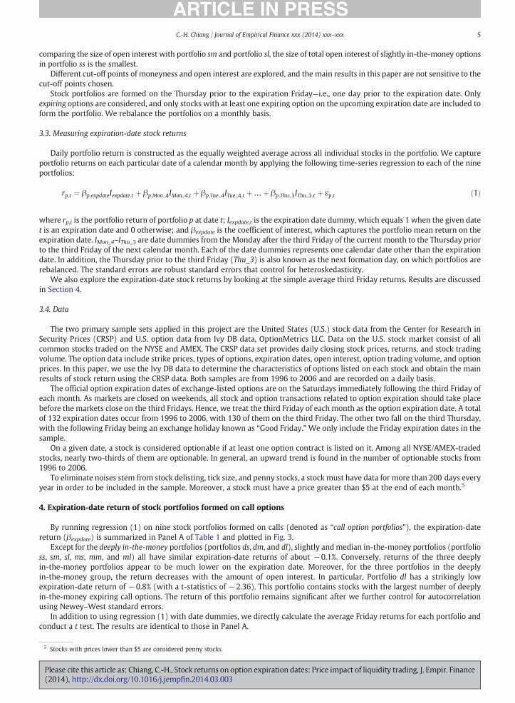
The option expiration date has long been a day with vibrant trading activities. In the option market, evidence shows (seeFig. 2) that the total open interest of options remains at a similar level in the expiration week. This fact suggests that mostinvestors wait until the expiration Friday to close their positions, and it gives rise to a large volume in the optionmarket. As for thestock market, empirical evidence also documents an enormous increase in stock trading volume (Chiang, 2009; Stoll andWhaley,1987, 1990).1 This is true not only for stocks with many at-the-money and slightly in-the-money options but also for those withplenty of deeply in-the-money options. Chiang (2009) further verifies the causal link between this large increase in tradingactivities and option expiration. When an option contract expires on Saturday, any position on this contract automaticallydisappears, and this change in option position can trigger parallel trading in the stock market and can offset trades to close out theoptions themselves on the third Friday (the last trading day before expiration). For stocks with most of their options being

he-money call options in each expiration week of 2006, with zero days to maturity as the expiration date

k returns on option expiration dates: Price impact of liquidity trading, J. Empir. Finance.2014.03.003

http://dx.doi.org/10.1016/j.jempfin.2014.03.003

mailto:[email protected]


http://www.sciencedirect.com/science/journal/09275398


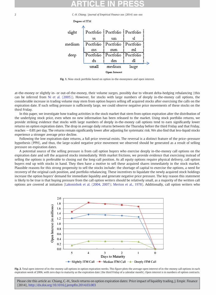
Fig. 1. Nine-stock portfolio based on option in-the-moneyness and open interest.

2 C.-H. Chiang / Journal of Empirical Finance xxx (2014) xxx–xxx

at-the-money or slightly in- or out-of-the-money, their volume surges, possibly due to vibrant delta-hedging rebalancing (thiscan be inferred from Ni et al. (2005)). However, for stocks with large numbers of deeply in-the-money call options, theconsiderable increase in trading volume may stem from option buyers selling off acquired stocks after exercising the calls on theexpiration date. If such selling pressure is sufficiently large, we could observe negative price movements of these stocks on thethird Friday.

In this paper, we investigate how trading activities in the stock market that stem from option expiration alter the distribution ofthe underlying stock price, even when no new information has been released to the market. Using stock portfolio returns, weprovide striking evidence that stocks with large numbers of deeply in-the-money call options tend to earn significantly lowerreturns on option expiration dates. The drop in average daily returns between the Thursday before the third Friday and that Friday,reaches−0.8% per day. The returns remain significantly lower after adjusting for systematic risk. We also find that less-liquid stocksexperience a stronger average price decline.

Following the low expiration-date returns, a full price reversal exists. The reversal is a distinct feature of the price–pressurehypothesis (PPH), and thus, the large-scaled negative price movement we observed should be generated as a result of sellingpressure on expiration dates.

A potential source of the selling pressure is from call option buyers who exercise deeply in-the-money call options on theexpiration date and sell the acquired stocks immediately. With market frictions, we provide evidence that exercising instead ofselling the options is preferable to closing out the long-call position. As all equity options require physical delivery, call optionbuyers end up with stocks in hand. They then have a motive to sell these acquired shares immediately in the stock market.Plausible reasons for this strong propensity to sell the stocks include: the shortage of capital to exercise the options, a need forrecovery of the original cash position, and portfolio rebalancing. These incentives to liquidate the newly acquired stock holdingsincrease the option buyers' demand for immediate liquidity and generate negative price pressure. The key reason this statementis likely to be true is that buying pressure from the call option writers should be relatively small, as a majority of the written calloptions are covered at initiation (Lakonishok et al. (2004, 2007); Merton et al., 1978). Additionally, call option writers who

Fig. 2. Total open interest of in-the-money call options in option expiration weeks. This figure plots the average open interest of in-the-money call options in eachexpiration week of 2006, with zero days to maturity as the expiration date (the third Friday of a calendar month). Open interest is in numbers of option contracts.

Please cite this article as: Chiang, C.-H., Stock returns on option expiration dates: Price impact of liquidity trading, J. Empir. Finance(2014), http://dx.doi.org/10.1016/j.jempfin.2014.03.003


3C.-H. Chiang / Journal of Empirical Finance xxx (2014) xxx–xxx

anticipate being assigned have an incentive to reduce the uncertainty of their losses by purchasing the underlying stocks beforethe expiration dates.2 Therefore, on option expiration dates, buying pressure tends to be negligible. We provide evidence thatwhen open interest of exercised calls is sufficiently large compared with the trading volume of the underlying stocks, the netselling pressure leads to a temporary drop in the returns of the underlying stocks.

This net selling pressure is not offset by potential put-option rebalancing, either. When we control for the put option openinterest by replacing the call option open interest with the net open interest (calls minus puts), the negative returns persist.Stocks with large amounts of net deeply in-the-money call option open interest experience an even larger daily drop in price,reaching −1.2%.

This paper contributes to the literature in several ways: First, it documents a significant return drop on option expiration datesfor stocks listed with large numbers of expiring deeply in-the-money call options. Second, we provide another empirical examplethat supports the price–pressure hypothesis and is cleaner in setup. A group of literature, such as that of Shleifer (1986), Harrisand Gurel (1986), and Wurgler and Zhuravskaya (2002), finds that a stock price rises when it is added into a stock index or whenits weight in an index increases. They attribute this phenomenon to an increase in demand for the stock, and the buying pressurepulls up the stock prices. However, because exchanges usually set certain criteria and only stocks that meet these criteria areadded to the indices, the addition (deletion) itself may convey information regarding the characteristics of the stock. The optionexpiration date, on the contrary, is completely exogenous, pre-determined, and publicly-known. It should contain no newinformation on the fundamentals. One may argue that certain information on the expiration date might result in pricemovements. Nonetheless, as the low returns on option expiration dates are recurrent, it is unlikely that similar information isreleased on a monthly basis and solely on the third Fridays. Third, this paper directly supports Huang and Wang (2009) andshares a similar non-informational implication as the 1987 crash, during which stock prices fell dramatically by 20% in a singletrading day without any news of obvious importance. Huang and Wang (2009) propose a theoretical model, according to whichthe need for liquidity is asymmetric, usually on the selling side and of large sizes. With a sudden surge in liquidity needs and alimited supply of capital to accommodate the trade imbalance, the excessive selling pressure drives prices to drop considerably,causing a market crash. The recovery, in terms of reversals, is slower than the drop in prices. This is mainly because the flow ofcapital into the market to provide liquidity is costly and thus takes time. Similarly, on option expiration dates, trading need isasymmetric, mostly from in-the-money call option buyers. With deeply in-the-money call option buyers selling the acquiredstocks, the prices of certain stocks drop temporarily below fundamentals. When capital flow is costly and slow, the followingreversal takes longer (a week in our sample) than the sudden drop in prices on expiration dates does. Apart from the role thatinformation plays with respect to price changes, this paper provides evidence of another channel through which selling pressureindirectly from a particular trading rule in the option market can lead to significant but rational price movements.

The remainder of the paper is organized as follows: In the next section, we review some related literature. In Section 3, wedescribe our methodology and samples. Section 4 reports the main results of expiration-date returns. An analysis of pricereversals is presented in Section 5. Section 6 provides potential sources of price pressure. Section 7 tests the robustness of theresults. Section 8 briefly discusses stock portfolios on put options, and Section 9 is the conclusion.

2. Related literature

Ever since the establishment of derivative markets three decades ago, the inter-market link between derivative markets andunderlying asset markets has been greatly discussed. One set of studies focuses on the impact of option introduction on theunderlying assets (e.g., Bansal et al., 1989; Conrad, 1989; Detemple and Jorion, 1990; Kumar et al., 1998; Mayhew and Mihov,2005; Skinner, 1989; Sorescu, 2000).

A relatively smaller number of studies examine the relation between option expiration and stock returns. Klemkosky (1978)investigates weekly returns before and after fourteen option expiration dates from 1975 to 1976, and he finds average abnormalreturns of −1% in the week before and +0.4% after the expiration date. However, he focuses on the weekly returns instead of onreturns on the expiration dates. Moreover, the positive returns in the week following option expiration are significant for onlythree of the 14 expiration dates. Cinar and Yu (1987) study the return behavior of six stocks on the expiration dates and findinsignificant results. The insignificance could be due to a considerably small sample of stocks. Instead, we apply daily returns witha much longer sample period (1996–2006) and include all optionable stocks traded on the NYSE/AMEX. Moreover, as optioncharacteristics such as types, in- or out-of-the-moneyness, and open interest may affect investors' trading strategies and thereforeaffect the direction and the size of price movement, we group stocks with similar option characteristics into portfolios andexamine their expiration-date returns.

This paper closely relates to Ni et al. (2005). They show that the closing prices of optionable stocks cluster to the nearest optionstrike prices on expiration dates, and they attribute such effect to portfolio rebalancing by option market makers. In Ni et al.(2005), the stock prices shift to the nearest strike prices. Therefore, this phenomenon should take place in stocks with largenumbers of close-the-money options (at-the-money, slightly in-the-money and slightly out-of-the-money options). However, in

2 To assign means to designate an option writer for fulfillment of his or her obligation to sell stocks (call option writer) or to buy stocks (put option writer).Assignment is the receipt of an exercise notice by an option writer that obligates him or her to sell (in the case of a call) or purchase (in the case of a put) theunderlying security at the specified strike price.




this paper, we discover that a significant return is in stocks with large numbers of deeply in-the-money options, and the effect isrestricted to call options.

3. Methodology and data

This section discusses how we form stock portfolios based on the characteristics of options listed on the relevant stock andhow we measure stock portfolio returns on the expiration date.

3.1. Option characteristics

The impact of options is three-folds—option types, moneyness, and open interest.Two types of options exist: call options and put options. Based on the security design and trading rules, calls and puts function

in opposite directions. For instance, on expiration dates when buyers exercise deeply in-the-money calls, they acquire underlyingstocks and sell them in the stock market, while for those who exercise deeply in-the-money puts, they purchase stocks and sellthem to put option writers. Given the fact that a majority of the writers are covered,3 exercising calls generates selling pressure(if any) in the stock market as exercising puts generates, on the contrary, buying pressure (if any). This inherent distinctioncauses different impacts on stock returns, and thus, these two types of options should be considered separately.

Moneyness is determined by the relative position of option strike price and current stock price. A call option is said to be in themoney (ITM) if its strike price is smaller than the underlying stock price; at-the-money (ATM) if equal; and out-of-the-money(OTM) if the strike is larger than the current stock price. For put options, the relation reverses. Different degrees of moneynesstend to give investors different trading strategies in both the stock and the option markets on expiration dates, and thesestrategies may further affect the direction of stock returns. In this paper, we only look at in-the-money options, as rationalinvestors do not exercise out-of-the-money options. Moreover, the duality of in-the-money calls (puts) and out-of-the-moneyputs (calls) makes the analyses of out-of-the-money options redundant. Stock portfolios based on OTM options are furtherdiscussed in Appendix A.

Open interest is defined as the total number of option contracts that are not closed or delivered on a particular day. If optionscarry useful information on the underlying stock, an option with larger open interest, which is equivalent to a larger share volumein the stock market, should have a stronger impact on stock returns than would an option with smaller open interest. Therefore,option interest should affect the size of stock price movements.

3.2. Forming stock portfolios

Different option characteristics give investors different trading strategies in the stock market, which may further generatedistinct return patterns. Thus, we group stocks into portfolios based on the three characteristics discussed in the previoussubsection of their options. This approach is distinct from prior studies, which apply individual returns. The portfolio approachalso helps to reduce noises.

After separate calls and puts, we apply a double-sortingmethodology. Individual stocks are first sorted based on the moneynessof their calls (puts) and then on the amount of open interest of their calls (puts).

Moneyness is the difference between the underlying stock price and the option strike price scaled by the underlying stockprice and described in percentages. We consider 0–5% ITM options slightly ITM, 5–25% ITM medium ITM, and options more than25% ITM are classified as deeply ITM. The 5% and 25% cut-off points are chosen so that for each stock, roughly one-third of theoptions are in each in-the-money category. We sort stocks into these three in-the-money groups based on the in-the-moneynessof their options. If a stock has more than one option listed on it and those options belong to different in-the-money groups, weallocate this stock into the in-the-money group with the largest total open interest. For instance, stock XYZ has five different calloptions with 1000 contracts outstanding: 200 contracts that are slightly ITM, 300 contracts that are medium ITM, and 500 that aredeeply ITM. As deeply in-the-money options have the largest total open interest in comparison with that of the slightly andmedium in-the-money ones, stock XYZ is classified as part of the deeply in-the-money group.

In each in-the-money group, we further sort the stock based on the total amount of open interest and form three other groups—small, medium, and large. The 40th and 70th percentiles of total open interest in each in-the-money class are used as cut-offpoints.4

Nine stock portfolios are based on calls and on puts, respectively, so 18 portfolios exist in total. All portfolios are denoted withtwo letters, as illustrated in Fig. 1. In particular, portfolio ss contains stocks that have a majority of their options as slightly ITM.When

3 Covered call writing is one of the most popular strategies among option investors. Merton et al. (1978) report that according to CBOE, 85% of all optionswritten are covered. This number is further supported by senior option practitioners.

4 The total amount of open interest only includes open interest of options in the in-the-money class in which the stock was classified; i.e., if a stock is classifiedin the deeply in-the-money class, the total open interest applied in the second-step sorting is calculated using all deeply in-the-money options listed under thisstock




comparing the size of open interest with portfolio sm and portfolio sl, the size of total open interest of slightly in-the-money optionsin portfolio ss is the smallest.

Different cut-off points of moneyness and open interest are explored, and the main results in this paper are not sensitive to thecut-off points chosen.

Stock portfolios are formed on the Thursday prior to the expiration Friday—i.e., one day prior to the expiration date. Onlyexpiring options are considered, and only stocks with at least one expiring option on the upcoming expiration date are included toform the portfolio. We rebalance the portfolios on a monthly basis.

3.3. Measuring expiration-date stock returns

Daily portfolio return is constructed as the equally weighted average across all individual stocks in the portfolio. We captureportfolio returns on each particular date of a calendar month by applying the following time-series regression to each of the nineportfolios:

5 Stoc

Pleas(201

rp;t ¼ βp;expdateIexpdate;t þ βp;Mon 4IMon 4;t þ βp;Tue 4ITue 4;t þ…þ βp;Thu 3IThu 3;t þ εp;t ð1Þ

rp,t is the portfolio return of portfolio p at date t; Iexpdate,t is the expiration date dummy, which equals 1 when the given date
wheret is an expiration date and 0 otherwise; and βexpdate is the coefficient of interest, which captures the portfolio mean return on theexpiration date. IMon_4–IThu_3 are date dummies from the Monday after the third Friday of the current month to the Thursday priorto the third Friday of the next calendar month. Each of the date dummies represents one calendar date other than the expirationdate. In addition, the Thursday prior to the third Friday (Thu_3) is also known as the next formation day, on which portfolios arerebalanced. The standard errors are robust standard errors that control for heteroskedasticity.
We also explore the expiration-date stock returns by looking at the simple average third Friday returns. Results are discussedin Section 4.

3.4. Data

The two primary sample sets applied in this project are the United States (U.S.) stock data from the Center for Research inSecurity Prices (CRSP) and U.S. option data from Ivy DB data, OptionMetrics LLC. Data on the U.S. stock market consist of allcommon stocks traded on the NYSE and AMEX. The CRSP data set provides daily closing stock prices, returns, and stock tradingvolume. The option data include strike prices, types of options, expiration dates, open interest, option trading volume, and optionprices. In this paper, we use the Ivy DB data to determine the characteristics of options listed on each stock and obtain the mainresults of stock return using the CRSP data. Both samples are from 1996 to 2006 and are recorded on a daily basis.

The official option expiration dates of exchange-listed options are on the Saturdays immediately following the third Friday ofeach month. As markets are closed on weekends, all stock and option transactions related to option expiration should take placebefore the markets close on the third Fridays. Hence, we treat the third Friday of each month as the option expiration date. A totalof 132 expiration dates occur from 1996 to 2006, with 130 of them on the third Friday. The other two fall on the third Thursday,with the following Friday being an exchange holiday known as “Good Friday.” We only include the Friday expiration dates in thesample.

On a given date, a stock is considered optionable if at least one option contract is listed on it. Among all NYSE/AMEX-tradedstocks, nearly two-thirds of them are optionable. In general, an upward trend is found in the number of optionable stocks from1996 to 2006.

To eliminate noises stem from stock delisting, tick size, and penny stocks, a stock must have data for more than 200 days everyyear in order to be included in the sample. Moreover, a stock must have a price greater than $5 at the end of each month.5

4. Expiration-date return of stock portfolios formed on call options

By running regression (1) on nine stock portfolios formed on calls (denoted as “call option portfolios”), the expiration-datereturn (βexpdate) is summarized in Panel A of Table 1 and plotted in Fig. 3.

Except for the deeply in-the-money portfolios (portfolios ds, dm, and dl), slightly andmedian in-the-money portfolios (portfolioss, sm, sl, ms, mm, and ml) all have similar expiration-date returns of about −0.1%. Conversely, returns of the three deeplyin-the-money portfolios appear to be much lower on the expiration date. Moreover, for the three portfolios in the deeplyin-the-money group, the return decreases with the amount of open interest. In particular, Portfolio dl has a strikingly lowexpiration-date return of −0.8% (with a t-statistics of −2.36). This portfolio contains stocks with the largest number of deeplyin-the-money expiring call options. The return of this portfolio remains significant after we further control for autocorrelationusing Newey–West standard errors.

In addition to using regression (1) with date dummies, we directly calculate the average Friday returns for each portfolio andconduct a t test. The results are identical to those in Panel A.

ks with prices lower than $5 are considered penny stocks.

e cite this article as: Chiang, C.-H., Stock returns on option expiration dates: Price impact of liquidity trading, J. Empir. Finance4), http://dx.doi.org/10.1016/j.jempfin.2014.03.003


Table 1Returns of nine itm call option portfolios on option expiration dates. This table reports the expiration-date average returns (Panel A) and risk-adjusted returns(Panel B) of nine stock portfolios formed on in-the-money call options. Expiration-date average return of each portfolio p is measured by regression coefficient(βexpdate) obtained by regressing equal-weighted portfolio returns on the date dummies:

rp;t ¼ βp;expdateIexpdate;t þ βp;Mon 4IMon 4;t þ βp;Tue 4ITue 4;t þ…þ βp;Thu 3IThu 3;t þ εp;t

Risk-adjusted returns of the nine in-the-money call option portfolios on option expiration dates are measured using the four-factor model. All returns are inpercentages. The t-statistics are adjusted for heteroskedasticity and reported in parentheses.

Open interest

In-the-moneyness Small Medium Large

Panel A: ITM call option portfoliosSlight −0.06 −0.08 −0.04

(−0.73) (−1.09) (−0.49)Medium −0.08 −0.14 −0.06

(−1.09) (−1.71) (−0.71)Deep −0.23 −0.41 −0.76

(−1.55) (−1.68) (−2.36)

Panel B: Risk-adjusted returnSlight 0 −0.03 0.04

(−0.09) (−0.87) (0.99)Medium −0.04 −0.07 0.04

(−1.30) (−2.42) (1.05)Deep −0.2 −0.36 −0.63

(−1.30) (−1.56) (−2.09)

Fig. 3. Returns of nine in-the-money call option portfolios on option expiration dates. This figure plots the equally weighted average returns of nine stockportfolios formed on in-the-money call options on option expiration dates. All returns are in percentages. Portfolio returns are obtained from Panel A of Table 1.


Fig. 4 compares portfolio returns on expiration dates with those on non-expiration Fridays and non-expiration dates. All nineportfolios have similar returns on dates other than on option expiration dates. Only on the expiration dates do stocks withsufficiently large numbers of deeply in-the-money call options earn considerably lower returns.

The first piece of evidence on the possible source of low expiration-date returns is the risk-based story. To explore, wecalculated the risk-adjusted returns by applying the four-factor model.6 After risk adjustments, as shown in Panel B of Table 1, thedeeply in-the-money portfolio with large amounts of open interest (aka Portfolio dl) consistently exhibits a significantly negativealpha of −0.7% (−2.17).

4.1. Value-weighted returns

Our main results discussed in the previous section use equal-weighted returns on a calendar date. In this subsection, weexplore the value-weighted returns on the expiration date. Panel A of Table 2 reports the average market capitalization of the nine

6 The four factor are the market premium factor (rmkt-rf), the size factor (SMB), the book-to-market factor (HML), and the momentum factor (MOM).



Fig. 4. Returns of nine in-the-money call option portfolios on expiration and non-expiration dates. This figure plots the average returns of nine in-the-money calloption portfolios on expiration dates, non-expiration Fridays and non-expiration dates. The average portfolio returns are regression coefficients obtaining byregressing daily portfolio returns on three sets of date dummies (expiration Friday, non-expiration Friday, and all other non-expiration date). All returns are inpercentages.

Table 2Market capitalization and value-weighted returns. This table reports the average market capitalization and value-weighted expiration-date returns of nine stockportfolios formed on in-the-money call options. Panel A reports the average market capitalization of the nine in-the-money call option portfolios. Panel B reportsthe value-weighted portfolio returns on the expiration date measured by regression (1). All returns are in percentages. The t-statistics are adjusted forheteroskedasticity and reported in parentheses.

Open interest


Panel A: Market capitalization (in millions)Slight 4191 9751 37,578Medium 3563 6739 24,840Deep 1978 5318 20,975

Panel B: Value-weighted portfolio returnSlight −0.08 −0.17 −0.09

(−0.99) (−2.09) (−0.98)Medium −0.08 −0.16 −0.02

(−1.09) (−1.85) (−0.29)Deep −0.43 −0.73 −1.40

(−1.59) (−2.20) (−2.27)


portfolios. Each individual stock in a given portfolio is weighted with its market capitalization relative to the total marketcapitalization of the relevant portfolio. We then apply Eq. (1) and report the value-weighted average expiration-date returns inPanel B of Table 2.

In Panel B, value-weighted returns show a similar pattern as do equal-weighted ones. Most of the slightly and medianin-the-money portfolios have insignificant returns except for portfolio ms. However, the magnitude is considerably smallercompared with the deeply in-the-money portfolios. Deeply in-the-money portfolios with median and large open interests show adip in returns: portfolio dm has a daily return of −0.7% (−2.2) and portfolio dl has a daily return of −1.4% (−2.27).

5. Price reversals

Stock portfolios with large numbers of expiring deeply in-the-money call options have significantly negative returns onexpiration dates. According to one potential hypothesis, call option buyers tend to exercise the options on option expiration dates.As physical settlement is required for equity options, call option buyers acquire stocks from option writers and immediately sellthe acquired shares in the stock market around the expiration date. This creates negative price pressure in the stock market andgenerates a price decline.

As the PPH predicts, a large-scaled sale (purchase) in a stock can result in price decreases (increases) even though no newinformation is associated with the transactions. Under PPH, the short-term demand curve for securities may not be perfectly



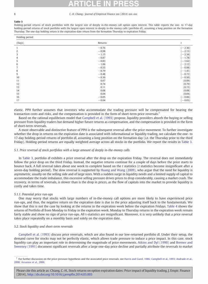
Table 3Holding-period returns of stock portfolios with the largest size of deeply in-the-money call option open interest. This table reports the one- to 17-dayholding-period returns of stock portfolio with the largest open interest in deeply in-the money calls (portfolio dl), assuming a long position on the formationThursday. The one-day holding return is the expiration-date return from the formation Thursday to expiration Friday.

Holding period

(Days) Returns t

1 −0.76 (−2.36)2 −0.98 (−2.13)3 −1.15 (−2.34)4 −0.87 (−1.78)5 −0.83 (−1.62)6 −1.06 (−2.12)7 −0.55 (−0.98)8 −0.79 (−1.41)9 −0.48 (−0.72)10 −0.36 (−0.50)11 0.07 (0.09)12 0.74 (0.79)13 0.11 (0.13)14 0.08 (0.08)15 0.04 (0.04)16 −0.05 (−0.06)17 −0.04 (−0.03)


elastic. PPH further assumes that investors who accommodate the trading pressure will be compensated for bearing thetransaction costs and risks, and the compensation is provided in the form of short-term price reversals.7

Based on the rational equilibrium model that Campbell et al. (1993) propose, liquidity providers absorb the buying or sellingpressure from liquidity traders but demand higher future returns as compensation, and the compensation is provided in the formof short-term reversals.

A most observable and distinctive feature of PPH is the subsequent reversal after the price movement. To further investigatewhether the drop in returns on the expiration date is associated with informational or liquidity trading, we calculate the one- to17-day holding-period returns of portfolio dl, assuming a long position on the formation day (i.e. the Thursday prior to the thirdFriday). Holding-period returns are equally weighted average across all stocks in the portfolio. We report the results in Table 3.

5.1. Price reversal of stock portfolios with a large amount of deeply in-the-money calls

In Table 3, portfolio dl exhibits a price reversal after the drop on the expiration Friday. The reversal does not immediatelyfollow the price drop on the third Friday. Instead, the negative returns continue for a couple of days before the price starts tobounce back. A full reversal takes about one week to complete based on the t statistics (t statistics become insignificant after aseven-day holding period). The slow reversal is supported by Huang and Wang (2009), who argue that the need for liquidity isasymmetric, usually on the selling side and of large sizes. With a sudden surge in liquidity needs and a limited supply of capital toaccommodate the trade imbalance, this excessive selling pressure drives prices to drop considerably, causing a market crash. Therecovery, in terms of reversals, is slower than is the drop in prices, as the flow of capitals into the market to provide liquidity iscostly and takes time.

5.1.1. Potential price run-upsOne may worry that stocks with large numbers of in-the-money call options are more likely to have experienced price

run-ups, and thus, the negative return on the expiration date is due to the price adjusting itself back to the fundamentals. Weshow that this is not the case by looking at the returns in the expiration week before the expiration Fridays. Table 4 shows thereturns of Portfolio dl from Monday to Friday in the expiration week. Monday to Thursday returns in the expiration week remainfairly stable and show no sign of price run-ups. All t-statistics are insignificant. Moreover, it is very unlikely that a price reversaltakes place repeatedly on a monthly basis and solely on the expiration date.

5.2. Stock liquidity and short-term reversals

Campbell et al. (1993) discuss price reversals, which are also found in our low-returned portfolio dl. Under their setup, thedemand curve for stocks may not be perfectly elastic, which allows trade pressure to induce a price impact. In this case, stockliquidity can play an important role in determining the magnitude of price movements. Atkins and Dyl (1990) and Bremer andSweeney (1991) document significant reversals after a large one-day price decline and partially attribute the reversals to market

7 For further discussion on the price-pressure hypothesis and the associated price reversals, see Harris and Gurel, 1986; Campbell et al., 1993; Andrade et al.,2008; Avramov et al., 2006.



Table 4Portfolio Returns in the Expiration Week. This table reports average returns of Portfolio dl from 5 days before expiration date to the expiration date. 0 is theexpiration date (the third Friday in a calendar month). −k is the k-th day prior to the expiration date, with k = 1 to 5. All returns are in percentages. Thet-statistics are adjusted for heteroskedasticity.

Days Return t

−5 0.09 (0.39)−4 0.20 (0.85)−3 0.33 (1.42)−2 0.29 (1.17)−1 −0.1 (−0.49)0 (expiration) −0.76 (−2.36)


illiquidity. Cox and Peterson (1994), who use firm size as a liquidity proxy, conclude that smaller firms tend to have strongerreversals. Avramov et al. (2006) also indicate that more illiquid stocks should have a steeper demand curve and accordinglyexperience stronger reversals.

In this subsection, we further sort stocks in portfolio dl into terciles based on liquidity. We apply the Amihud illiquidity ratio(Amihud, 2002) to measure stock illiquidity. The Amihud illiquidity ratio for stock i at date t, ILLIQi,t, is defined as the ratio of itsdaily absolute returns to its daily dollar trading volume:

Table 5Expiratinto tercapture

Illiqu

1

−0.0(−0.2

Pleas(201

ILLIQi;t ¼ri;t�� VOLi;t

: ð2Þ

� �
Illiquidity of individual stock i at each date t is further measured as its past-week average ILLIQi;t .
Table 5 summarizes the average expiration-date return in the three liquidity terciles, respectively. The more illiquid a stock is,the larger the illiquidity ratio. Consistent with Avramov et al. (2006), less-liquid stocks experience stronger price drops. Tercile 3,which includes the most illiquid stocks, drops by 2.38% more in returns on the expiration date than tercile 1 does.

6. Sources of negative price pressure

The expiration-date price movement is not permanent but instead is accompanied by a complete reversal. This supports theprice–pressure hypothesis and suggests that the drop in returns on the expiration date is associated with the selling pressure. Thisresult raises a question of what produces the selling pressure on the expiration date.

A potential interpretation of the low return in stocks with a sufficiently large number of deeply in-the-money call options onoption expiration dates is as follows:

Investors with a long position on deeply ITM call options tend to exercise the options on the expiration date. With the physicalsettlement feature of equity options, these call option buyers acquire stocks and sell them immediately in the stock market. Whenthe open interest of exercised calls is sufficiently large compared to the daily trading volume of the underlying stocks, this“exercise-and-sell” trade generates downward selling pressure in the stock market. As a majority of the option writers are hedgedby writing covered calls, the buying pressure from the writers is relatively small. Due to this non-synchronization betweenbuying and selling the underlying stocks, there is “net selling pressure” in the stock market on the expiration date, which resultsin a drop in returns.

We further discuss the rationales and provide supporting evidence in the following subsections.

6.1. Do call option buyers exercise at maturity?

The first assumption of this “selling pressure” story is that investors need to exercise in-the-money call options on theexpiration date. Evidence shows (as in Fig. 2) that the total open interest of in-the-money call options remains stable throughout

ion-date returns and stock liquidity. This table reports average expiration-date returns in three illiquidity terciles. We further sorting stocks portfolio dlciles based on the past-week average Amihud illiquidity ratio. Tercile 1 includes the most liquid stocks and tercile 3 includes the most illiquid stocks. “3–1”s the difference in returns between the two most extreme terciles. All returns are in percentages. The t-statistics are adjusted for heteroskedasticity.

idity

2 3 “3–1”

4 −0.53 −2.43 −2.38) (−1.59) (−2.28) (−2.19)




the expiration week. This suggests that investors do not liquidate the option position in the expiration week before the thirdFriday, andmost of the open interest is carried to the expiration date. This is true even for options already being deeply ITM beforethe expiration Friday.8 With these carried-over call options, investors have two alternatives for closing the position on the thirdFriday—exercising them or selling them.

Finucane (1997) and Overdahl and Martin (1994) study the exercise behavior and show that investors tend to exercise theoption with the existence of market frictions, such as a large option bid-ask spread. Accordingly, if a comparably larger spreadexists in the option market than in the stock market, investors would have incentives to exercise the option and trade theunderlying stocks in the stock market. By looking at the bid-ask spread from 90 days prior to expiration to the expiration date, asshown in Fig. 5, a dramatic increase in the in-the-money call option spread occurs as the expiration date approaches. The spread iseven wider for deeply in-the-money calls. The wide spread indicates a relatively illiquid option market. This is true when we lookat the bid-ask spread in raw number without scaling. We also consider the unscaled bid-ask spread because it is the actualtransaction cost that investors are facing when they exercise the options. Similarly, as in Fig. 6, unscaled bid-ask spread of deeplyITM call options9 increases continuously from two weeks before the expiration to the expiration date. With the existence of awide option spread compared with that in the stock market, investors might be better off by exercising the option and trading theacquired stocks rather than selling the calls. Therefore, we further compare the profits from two of the following trading strategieson option expiration dates by taking into consideration the transaction cost (in terms of bid-ask spread) in both markets:

1. Exercise Options and Sell Stocks: Exercise an in-the-money call option at the strike price and sell the underlying stock at theexpiration-date bid price. The profit (π ) of this strategy is

8 Bycontrac5%. Thisonly a 1third Thoption i

9 We

Pleas(201

π1 ¼ stock bid−strike priceð Þfor acalloption ð3Þ

2. Close by Selling Options: Close the option position by selling the option at the bid price of the day, and the profit (π ) is

π2 ¼ option bid: ð4Þ

We then calculate the difference between π and π , denoted by πdiff, and present the result in Table 6. πdiff is scaled by theclosing price of the underlying stock and is reported in percentages.

In Panel A of Table 6, πdiff is significantly positive for medium and deeply in-the-money options, with the magnitude beingparticularly large for deeply in-the-money options. After considering the transaction cost in the stock market, “Exercise Optionsand Sell Stocks” still generates 0.42% higher profits per share for deeply in-the-money calls. This is due partly to a largerpercentage of option in-the-moneyness and partly to a wider option spread.

Panel B further explores πdiff in each of the nine in-the-money call option portfolios. For each portfolio, only πdiff from tradingoptions in the same in-the-money group are reported. For instance, for the three deeply in-the-money portfolios, only profits oftrading deeply in-the-money options are reported. For all of the three deeply in-the-money portfolios, exercising the deeplyin-the-money call options listed under the stocks in these portfolios generate statistically significant higher profits. Byconstruction, the majority of options listed under these portfolios are deeply ITM. Therefore, investors should have incentives toexercise a majority of the call options listed under stocks in these portfolios.

To conclude, with market frictions, the “Exercise Options and Sell Stocks” strategy outperforms the “Close by Selling Options”strategy, and this provides investors with incentives to exercise the call options on expiration dates.

Moreover, Poteshman and Serbin (2003) point out that when investors become involved in the irrational early exercise of calloptions, more often, the underlying stock is attaining a historically high price or is earning a high return. This implies that a highprice of the underlying stock can trigger investors to exercise the option. When a call option is classified as deeply ITM, theunderlying stock is reaching a relatively higher price, and this higher share price provokes investors to exercise the call option.Different from the irrational early exercise, these transactions should be considered a rational exercise on the expiration date.

In summary, in the expiration week, few option contracts are closed before the expiration date. On the expiration date,investors face higher transaction costs in the form of a wider spread in the option market. The large spread makes exercising theoption and selling the acquired underlying stock a dominant trading strategy.

6.2. Call option buyers sell acquired stock immediately

Based on the previous discussion, call option buyers have incentives to exercise the calls. Because equity options require physicaldelivery, these option buyers acquire stocks from option writers. Then, they sell these acquired underlying stocks immediately in thestock market. Senior option traders further confirm this statement. We provide some rationales.

calculating the change in total in-the-money option open interest in the expiration week, call option open interest decreases by only 4.12% (41,600ts) from the third Thursday to the expiration Friday. As for deeply in-the-money call options (determined as deeply ITM on Thursday), the decrease is onlysuggests that most of the open interest is carried to the expiration date. In-the-money put options have an even smaller change in open interest, with.98% decrease from the Thursday prior to the third Friday to the third Friday. The change in open interest is much smaller from the third Wednesday to theursday, with a 1.62% decrease for calls and a 1.14% decrease for puts. This evidence shows that investors wait until the expiration date even though thes already deeply ITM before the expiration Friday.only consider the deeply in-the-money call options here because abnormal returns are observed only in stocks with a large portion of deeply ITM calls.



Fig. 5. Option and stock spreads. This figure plots both the call option spread and the stock spread from 90 days before expiration to the expiration date. Bothspreads are calculated as the bid-ask spread scaled by the midpoint.


Investors have several justifications for their motives to sell the stocks immediately. First of all, to exercise call options,investors require capital to purchase shares from option writers. As the trading hour and settlement period for both the stock andthe option markets are synchronized, with a possible capital constraint, investors need to sell the stocks simultaneously in orderto raise sufficient capital on the expiration date. Second, if a subset of investors wants to recover the cash position when their calloptions expire, they can do so via selling the acquired stocks. Third, some investors hold diversified portfolios, with a fixedfraction being allocated to certain types of stocks, and they are exposed to a larger risk if the fraction on a single stock suddenlyrises. After acquiring the underlying stocks, the weight of their diversified portfolios on certain stocks increases. For riskconsideration, they might rebalance their portfolio holdings by selling the additional stocks.

All in all, these are potential actions that investors take around option expiration dates. This increases the demand forimmediate liquidity. The resulting selling pressure leads to a drop in portfolio returns on option expiration dates. Because therecovery of cash position and portfolio rebalance need not take place solely on the expiration date, they serve as a plausibleexplanation for a temporary price continuation on Monday following the expiration date. The price decline, in turn, attracts thepassive liquidity suppliers. This price movement subsequently reverses as a compensation for the liquidity providers.

6.3. Net selling pressure

For the selling pressure to have a negative price impact, the corresponding buying pressure from the writer must be negligible.If a majority of the option writers need to purchase stocks in order to deliver, this corresponding buying pressure could offset theselling pressure and result in insignificant price movement.

Fig. 6. Option bid-ask spreads. This figure plots both the call option spread and the stock spread from two weeks before expiration to the expiration date. Thebid-ask spreads are calculated as the difference between the ask and the bid prices.



Table 6Profits from two trading strategies on option expiration dates. This table reports the difference in trading profits (πdiff) from two trading strategies—ExerciseOptions and Sell Stocks and Close by Selling Options—on option expiration dates. πdiff is defined as the difference between π and π , where π is the profit from theExercise Options at strike and Sell Stocks at bid strategy, and π is that from the Close by Selling Options at bid strategy. Panel A reports πdiff in three moneynessgroups. Panel B reports πdiff in nine in-the-money call option portfolios.

Panel A: Three ITM groups and two types of options

In-the-moneyness

Type Slight Medium Deep

Call −0.08% 0.11% 0.42%(−13.56) (14.2) (4.24)

Put −0.07% 0.08% 0.70%(−10.92) (10.63) (4.61)

Panel B: Trading profits of nine portfolios

Open interest


Slight −0.07% −0.05% −0.08%(−0.96) (−0.78) (−1.03)

Medium −0.01% 0.13% 0.01%(−0.14) (1.69) (0.16)

Deep 1.58% 1.35% 1.02%(5.56) (4.01) (2.94)


Merton et al. (1978) report that according to CBOE, 85% of all options written are covered.10 This fact indicates that most of thewriters simultaneously purchase the underlying stocks while writing call options. Lakonishok et al. (2004, 2007) further confirmthis. They provide evidence that investors who write calls tend to own the underlying common stock, that is, they write coveredcalls. Moreover, for deeply in-the-money calls, a writer can rationally anticipate before the expiration date that the option will beexercised with a reasonably high probability. In accordance, the writer's purchase of stocks in preparation for potential futuredelivery spreads out across days before option expiration instead of concentrating solely on the expiration date. Therefore, thebuying pressure from writers on the expiration date should be relatively negligible compared with the selling pressure from thecall option buyers. As a result, net selling pressure is present in the stock market, which pushes down the price.

6.4. Selling pressure versus stock trading volume

With strong net selling pressure, stock prices fall on option expiration dates, as documented in this paper. In the following, wetry to explain why low returns are only observed in stocks with sufficiently large numbers of deeply ITM calls:

1. Deeply in-the-money call options, on average, have a wider spread. Combined with a relatively higher price, this givesinvestors a stronger motive to exercise the option (as suggested by Table 6).

2. However, to generate downward price pressure, the key is the volume of the sale orders. In other words, option open interestneeds to be large compared with the daily trading volume of the underlying stock in order to move the stock market.With a standardized contract, one call option contract gives investors the right to purchase 100 shares of the underlying stock.In other words, when an investor exercises the call option, for one contract, he or she receives 100 shares of the underlyingstock. To generate sufficient pressure to drive the price down, when investors sell the acquired shares, the number of sharesshould be large enough compared with the daily trading volume of the stock. For instance, if call option XYZ is 50% ITM,investors may lower the selling price of the underlying stock by 20%. The total option interest of XYZ, however, is only onecontract (which is equivalent to 100 stock shares), while the daily trading volume of the underlying stock is 1 million shares.Selling these 100 stock shares clearly cannot shift the market price.Panel A of Table 6 shows the ratios of call option open interest to the daily trading volume of the underlying stocks. Open interestwe apply here is calculated by converting the original open interest into equivalent stock shares (one option contract is worth 100shares of the underlying stock). Daily trading volume of stocks is measured in share volume. Stock portfolios without lowexpiration-date returns have not only smaller degrees of moneyness but also much smaller open-interest-to-trading-volumeratios. On the contrary, the low-returned portfolios (portfolio dl, in particular) have much larger open-interest-to-volume ratioswhile compared with other portfolios. Moreover, as the ratio increases from 4.53% (portfolio dm) to 40.06% (portfolio dl),portfolio returns also drop from−0.41% to−0.76% (as documented in Section 4), indicating a stronger negative impact on price.

10 This number is further supported by senior option practitioners.



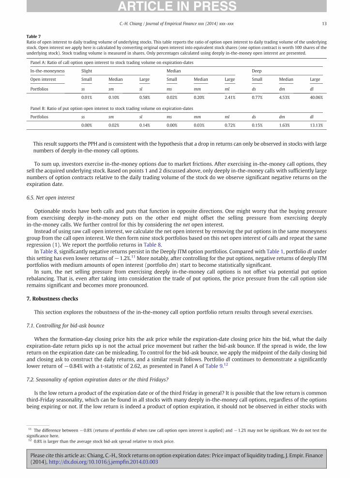
Table 7Ratio of open interest to daily trading volume of underlying stocks. This table reports the ratio of option open interest to daily trading volume of the underlyingstock. Open interest we apply here is calculated by converting original open interest into equivalent stock shares (one option contract is worth 100 shares of theunderlying stock). Stock trading volume is measured in shares. Only percentages calculated using deeply in-the-money open interest are presented.

Panel A: Ratio of call option open interest to stock trading volume on expiration-dates

In-the-moneyness Slight Median Deep

Open interest Small Median Large Small Median Large Small Median Large

Portfolios ss sm sl ms mm ml ds dm dl

0.01% 0.10% 0.58% 0.02% 0.20% 2.41% 0.77% 4.53% 40.06%

Panel B: Ratio of put option open interest to stock trading volume on expiration-dates

Portfolios ss sm sl ms mm ml ds dm dl

0.00% 0.02% 0.14% 0.00% 0.03% 0.72% 0.15% 1.63% 13.13%


This result supports the PPH and is consistent with the hypothesis that a drop in returns can only be observed in stocks with largenumbers of deeply in-the-money call options.

To sum up, investors exercise in-the-money options due to market frictions. After exercising in-the-money call options, theysell the acquired underlying stock. Based on points 1 and 2 discussed above, only deeply in-the-money calls with sufficiently largenumbers of option contracts relative to the daily trading volume of the stock do we observe significant negative returns on theexpiration date.

6.5. Net open interest

Optionable stocks have both calls and puts that function in opposite directions. One might worry that the buying pressurefrom exercising deeply in-the-money puts on the other end might offset the selling pressure from exercising deeplyin-the-money calls. We further control for this by considering the net open interest.

Instead of using raw call open interest, we calculate the net open interest by removing the put options in the same moneynessgroup from the call open interest. We then form nine stock portfolios based on this net open interest of calls and repeat the sameregression (1). We report the portfolio returns in Table 8.

In Table 8, significantly negative returns persist in the Deeply ITM option portfolios. Compared with Table 1, portfolio dl underthis setting has even lower returns of−1.2%.11 More notably, after controlling for the put options, negative returns of deeply ITMportfolios with medium amounts of open interest (portfolio dm) start to become statistically significant.

In sum, the net selling pressure from exercising deeply in-the-money call options is not offset via potential put optionrebalancing. That is, even after taking into consideration the trade of put options, the price pressure from the call option sideremains significant and becomes more pronounced.

7. Robustness checks

This section explores the robustness of the in-the-money call option portfolio return results through several exercises.

7.1. Controlling for bid-ask bounce

When the formation-day closing price hits the ask price while the expiration-date closing price hits the bid, what the dailyexpiration-date return picks up is not the actual price movement but rather the bid-ask bounce. If the spread is wide, the lowreturn on the expiration date can be misleading. To control for the bid-ask bounce, we apply the midpoint of the daily closing bidand closing ask to construct the daily returns, and a similar result follows. Portfolio dl continues to demonstrate a significantlylower return of −0.84% with a t-statistic of 2.62, as presented in Panel A of Table 9.12

7.2. Seasonality of option expiration dates or the third Fridays?

Is the low return a product of the expiration date or of the third Friday in general? It is possible that the low return is commonthird-Friday seasonality, which can be found in all stocks with many deeply in-the-money call options, regardless of the optionsbeing expiring or not. If the low return is indeed a product of option expiration, it should not be observed in either stocks with

11 The difference between −0.8% (returns of portfolio dl when raw call option open interest is applied) and −1.2% may not be significant. We do not test thesignificance here.12 0.8% is larger than the average stock bid-ask spread relative to stock price.



Table 9Robustness checks. This table reports results of robustness checks on in-the-money call option portfolio returns. Panel A reports the expiration-date returnsconstructed by using the daily midpoint; Panel B reports expiration-date portfolio returns after removing the triple-witching days; Panel C reportsexpiration-date returns after removing the LEAPS. All returns are measured using Eq. (1) and are reported in percentages. The t-statistics are adjusted forheteroskedasticity and reported in parentheses.

Open interest


Panel A: ITM call option portfolio returns constructed using midpointSlight −0.05 −0.09 −0.09

(−0.68) (−1.08) (−1.03)Medium −0.06 −0.14 −0.06

(−0.75) (−1.81) (−0.69)Deep −0.04 −0.33 −0.84

(−0.29) (−1.30) (−2.62)

Panel B: ITM call option portfolio returns on non-triple-witching expiration datesSlight −0.06 −0.08 −0.07

(−0.64) (−0.77) (−0.57)Medium −0.11 −0.16 −0.09

(−1.10) (−1.46) (−0.87)Deep −0.26 −0.34 −0.97

(−1.29) (−1.06) (−2.80)

Panel C: ITM call option portfolio returns after removing LEAPSSlight −0.06 −0.10 −0.06

(−0.72) (−1.20) (−0.60)Medium −0.09 −0.15 −0.07

(−1.18) (−1.79) (−0.78)Deep −0.15 −0.42 −0.81

(−1.19) (−1.56) (−2.33)

Table 8Returns of ITM call option portfolios based on net open interest. This table reports the expiration-date returns of nine stock portfolios formed on in-the-moneycall options. Open interest is in net value, which is calculated by removing the put options in the same moneyness group from the call option open interest.Expiration-date return of each portfolio is measured by regression (1). All returns are in percentages. The t-statistics are adjusted for heteroskedasticity andreported in parentheses.

Returns of ITM call option portfolio based on net open interest

Net open interest


Slight −0.06 −0.01 0.00(−0.85) (−0.15) (0.00)

Medium −0.02 −0.06 −0.01(−0.28) (−0.87) (−0.15)

Deep −0.13 −0.53 −1.20(−0.47) (−2.68) (−2.95)


non-expiring options or nonoptionable stocks. Hence, we further examine these two alternative sets of stocks. Optionable stocksare double-sorted into nine portfolios based on the characteristics of non-expiring call options, while nonoptionable stocks aregrouped into a single portfolio. Notice that almost all optionable stocks have both expiring and non-expiring options. The onlydifference here is that for Table 1, stocks are sorted based on the characteristics of “expiring” options, while here, stocks are sortedbased on “non-expiring” options, regardless of their maturity. The result shows that the third-Friday returns using these twosamples are insignificant. This implies that the low return stem from activities that take place only in the expiring options andonly on the expiration date.

7.3. Expiration of index futures—the triple-witching day

Index futures also expire on the third Fridays. However, instead of a monthly expiration scheme, index futures expire on aquarterly basis. To ensure that the low returns are not generated from the expiration of index futures, we remove all quarterlyexpiration dates before forming the portfolios.13 The result remains the same (Panel B of Table 9).

13 Index futures contracts expire on the third Friday of March, June, September, and December—the so-called triple-witching day.



Table 10Risk-adjusted returns of nine in-the-money put option portfolios on option expiration dates. This table reports the reports the expiration-date risk-adjustedreturns of nine stock portfolios formed on in-the-money put options. Expiration-date risk-adjusted returns of the nine in-the-money put option portfolios aremeasured using the four-factor model. All returns are in percentages. The t-statistics are adjusted for heteroskedasticity and reported in parentheses.

ITM put option portfolio risk-adjusted returns

Open interest


Slight −0.07 −0.04 −0.04(−2.30) (−1.15) (−0.93)

Medium −0.01 −0.02 −0.05(−0.29) (−0.36) (−1.06)

Deep 0.18 −0.2 −0.21(1.68) (−1.68) (−1.33)

Fig. 7. Total open interest. This figure plots the total open interest of call options and put options from 180 days before expiration to the expiration date. Openinterest is in numbers of option contracts.


7.4. Expiration of LEAPS

Long-Term Equity Anticipation Securities (LEAPS), known as the long-term equity option contracts, expire only in January.After we remove the January expiration dates, all portfolios exhibit a similar expiration-date return pattern, suggesting that thelow-return effect is not confined to the LEAPS expiration date but to a widespread phenomenon for stocks with equity options(Panel C of Table 9).

8. Expiration-date returns of put option portfolios

This section briefly discusses the expiration-date returns of nine stock portfolios formed on the put options. Here, we reportthe risk-adjusted returns measured by the four-factor model in Table 10. All assumptions are the same as those applied to the calloption portfolios.

All put option portfolios have statistically close to zero risk-adjusted returns on the expiration dates. When compared withreturns of deeply in-the-money call option portfolios, the magnitude of put option portfolio returns is considerably smaller, withthe largest one being only 0.2%. This is due to the fact that the size of open interest of put options compared with the daily tradingvolume of the underlying stocks is too small to generate sufficient price pressure (Panel B of Table 7).

In general, put options have much smaller open interest than do calls throughout the entire option duration. This is shown inFig. 7, which plots the total open interest of in-the-money calls and in-the-money puts from 180 days before expiration to theexpiration date using the 1996—2006 sample. Put options start with a considerably smaller open interest than calls by more than46%. The gap widens as the expiration date approaches. The same pattern follows by using only the 2006 sample. Additionally, asmaller fraction of put options than calls are exercised on the expiration date (40% compared with 70%), giving rise to an evensmaller proportion of stock shares from put options in the stock market.14 This smaller friction is also consistent with the option

14 The percentages are documented in Finucane (1997) and Overdahl and Martin (1994).




pricing theory, according to which call options should optimally be exercised prior to maturity if and only if the underlying stockis about to pay a sufficiently large cash dividend. The same does not apply to put options, which implies that the exercise of putoptions spreads out across the option duration.

9. Conclusion

In this paper, we first provide striking evidence that, by forming stock portfolios based on option characteristics, stocks withsufficiently large numbers of expiring deeply in-the-money call options earn significantly lower returns on monthly optionexpiration dates. This negative return has a considerably large magnitude, with an average daily drop of up to 0.8% and remainssignificant after adjusting for systematic risk.

The drop in returns is followed by a full reversal. This price reversal supports the price–pressure hypothesis, according towhich the large selling pressure generates the low return. On option expiration dates, investors with a long position in the optionmarket tend to exercise their deeply in-the-money call options and sell the acquired shares immediately in the stock market. Thisincreasing demand for immediacy results in selling pressure in the stock market. As a majority of the option writers are hedged bywriting covered calls, the buying pressure from the writers is relatively small. This non-synchronization between buying andselling the underlying stocks creates net selling pressure on the expiration date and results in a drop in stock returns. Thisnegative selling pressure is not offset by portfolio rebalancing of put options on the opposite end, as the significant negativereturns persist after considering the net open interest.

The price subsequently reverses, generating higher future returns as a compensation for liquidity suppliers. The drop inexpiration-date price and the further reversal provide empirical support to Campbell et al. (1993) and Huang and Wang (2009).

Appendix A

A.1. OTM option portfolios

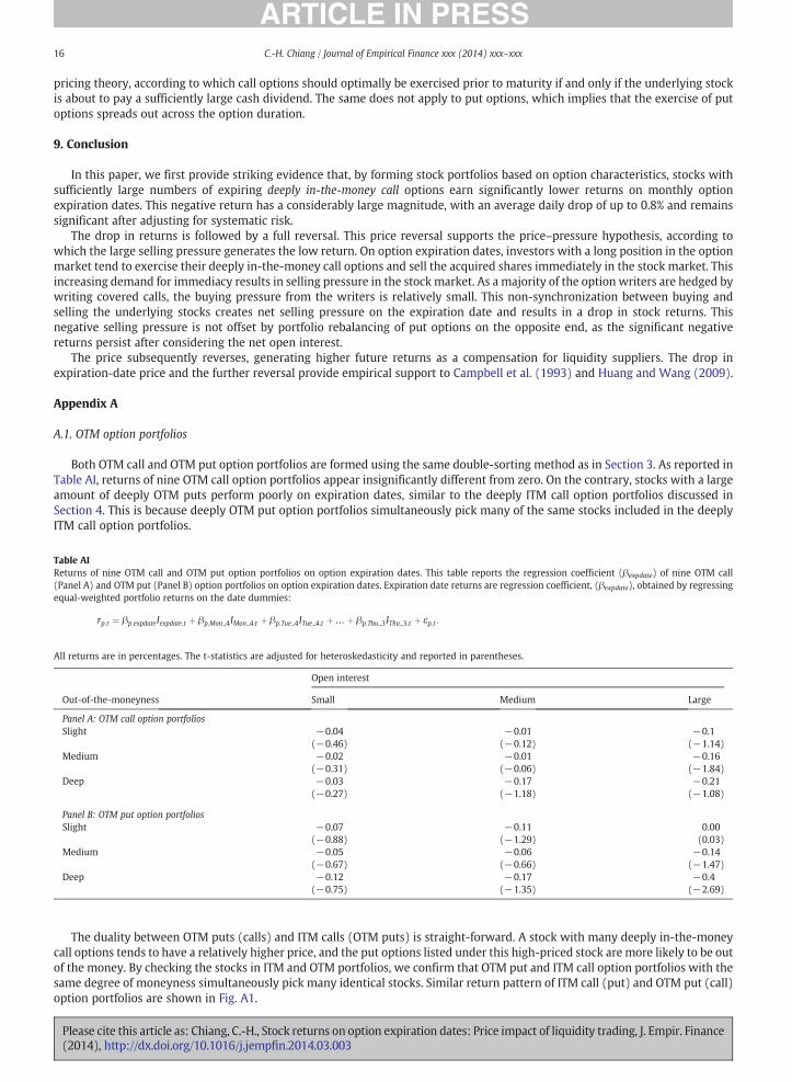
Both OTM call and OTM put option portfolios are formed using the same double-sorting method as in Section 3. As reported inTable AI, returns of nine OTM call option portfolios appear insignificantly different from zero. On the contrary, stocks with a largeamount of deeply OTM puts perform poorly on expiration dates, similar to the deeply ITM call option portfolios discussed inSection 4. This is because deeply OTM put option portfolios simultaneously pick many of the same stocks included in the deeplyITM call option portfolios.

Table AIReturns of nine OTM call and OTM put option portfolios on option expiration dates. This table reports the regression coefficient (βexpdate) of nine OTM call(Panel A) and OTM put (Panel B) option portfolios on option expiration dates. Expiration date returns are regression coefficient, (βexpdate), obtained by regressingequal-weighted portfolio returns on the date dummies:

rp;t ¼ βp;expdateIexpdate;t þ βp;Mon 4IMon 4;t þ βp;Tue 4ITue 4;t þ…þ βp;Thu 3IThu 3;t þ εp;t :

All returns are in percentages. The t-statistics are adjusted for heteroskedasticity and reported in parentheses.

Open interest

Out-of-the-moneyness Small Medium Large

Panel A: OTM call option portfoliosSlight −0.04 −0.01 −0.1

(−0.46) (−0.12) (−1.14)Medium −0.02 −0.01 −0.16

(−0.31) (−0.06) (−1.84)Deep −0.03 −0.17 −0.21

(−0.27) (−1.18) (−1.08)

Panel B: OTM put option portfoliosSlight −0.07 −0.11 0.00

(−0.88) (−1.29) (0.03)Medium −0.05 −0.06 −0.14

(−0.67) (−0.66) (−1.47)Deep −0.12 −0.17 −0.4

(−0.75) (−1.35) (−2.69)

The duality between OTM puts (calls) and ITM calls (OTM puts) is straight-forward. A stock with many deeply in-the-moneycall options tends to have a relatively higher price, and the put options listed under this high-priced stock are more likely to be outof the money. By checking the stocks in ITM and OTM portfolios, we confirm that OTM put and ITM call option portfolios with thesame degree of moneyness simultaneously pick many identical stocks. Similar return pattern of ITM call (put) and OTM put (call)option portfolios are shown in Fig. A1.



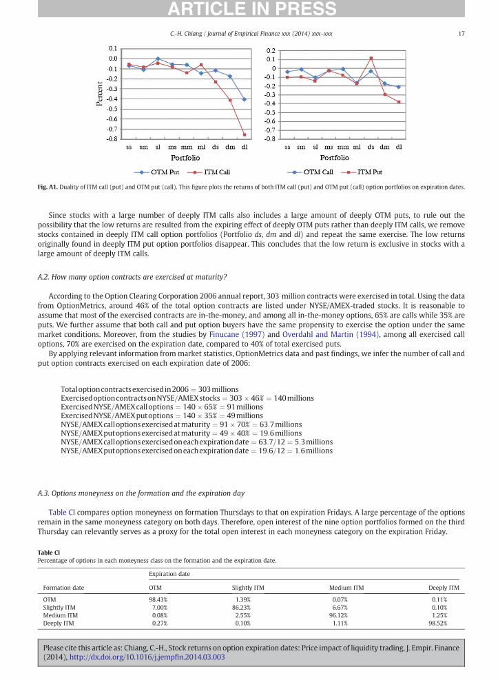
Fig. A1. Duality of ITM call (put) and OTM put (call). This figure plots the returns of both ITM call (put) and OTM put (call) option portfolios on expiration dates.


Since stocks with a large number of deeply ITM calls also includes a large amount of deeply OTM puts, to rule out thepossibility that the low returns are resulted from the expiring effect of deeply OTM puts rather than deeply ITM calls, we removestocks contained in deeply ITM call option portfolios (Portfolio ds, dm and dl) and repeat the same exercise. The low returnsoriginally found in deeply ITM put option portfolios disappear. This concludes that the low return is exclusive in stocks with alarge amount of deeply ITM calls.

A.2. How many option contracts are exercised at maturity?

According to the Option Clearing Corporation 2006 annual report, 303 million contracts were exercised in total. Using the datafrom OptionMetrics, around 46% of the total option contracts are listed under NYSE/AMEX-traded stocks. It is reasonable toassume that most of the exercised contracts are in-the-money, and among all in-the-money options, 65% are calls while 35% areputs. We further assume that both call and put option buyers have the same propensity to exercise the option under the samemarket conditions. Moreover, from the studies by Finucane (1997) and Overdahl and Martin (1994), among all exercised calloptions, 70% are exercised on the expiration date, compared to 40% of total exercised puts.

By applying relevant information frommarket statistics, OptionMetrics data and past findings, we infer the number of call andput option contracts exercised on each expiration date of 2006:

Table CPercent

Form

OTMSlightMediDeep

Pleas(201

Totaloptioncontractsexercisedin2006 ¼ 303millionsExercisedoptioncontractsonNYSE=AMEXstocks ¼ 303� 46% ¼ 140millionsExercisedNYSE=AMEXcalloptions ¼ 140� 65% ¼ 91millionsExercisedNYSE=AMEXputoptions ¼ 140� 35% ¼ 49millionsNYSE=AMEXcalloptionsexercisedatmaturity ¼ 91� 70% ¼ 63:7millionsNYSE=AMEXputoptionsexercisedatmaturity ¼ 49� 40% ¼ 19:6millionsNYSE=AMEXcalloptionsexercisedoneachexpirationdate ¼ 63:7=12 ¼ 5:3millionsNYSE=AMEXputoptionsexercisedoneachexpirationdate ¼ 19:6=12 ¼ 1:6millions

A.3. Options moneyness on the formation and the expiration day

Table CI compares option moneyness on formation Thursdays to that on expiration Fridays. A large percentage of the optionsremain in the same moneyness category on both days. Therefore, open interest of the nine option portfolios formed on the thirdThursday can relevantly serves as a proxy for the total open interest in each moneyness category on the expiration Friday.

Iage of options in each moneyness class on the formation and the expiration date.

Expiration date

ation date OTM Slightly ITM Medium ITM Deeply ITM

98.43% 1.39% 0.07% 0.11%ly ITM 7.00% 86.23% 6.67% 0.10%um ITM 0.08% 2.55% 96.12% 1.25%ly ITM 0.27% 0.10% 1.11% 98.52%




References

Amihud, Yakov, 2002. Illiquidity and stock returns: cross-section and time-series effects. J. Financ. Mark. 5 (1), 31–56.Andrade, Sandro C., Chang, Charles, Seasholes, Mark S., 2008. Trading imbalances, predictable reversals, and cross-stock price pressure. J. Financ. Econ. 88 (2),

406–423.Atkins, A.B., Dyl, E.A., 1990. Price reversals, bid-ask spreads, and market efficiency. J. Financ. Quant. Anal. 25 (O4), 535–547.Avramov, D., Chordia, T., Goyal, A., 2006. Liquidity and autocorrelations in individual stock returns. J. Financ. 61 (5), 2365–2394.Bansal, Vipul, Pruitt, Stephen W., Wei, John, 1989. An empirical reexamination of the impact of CBOE option initiation on the volatility and trading volume of the

underlying equities: l973—1986. Financ. Rev. 24.Bremer, M., Sweeney, R.J., 1991. The reversal of large stock-price decreases. J. Financ. 46 (2), 747–754.Campbell, John Y., Grossman, S.J., Wang, J., 1993. Trading volume and serial correlation in stock returns. Q. J. Econ. 108 (4), 905–939.Chiang, Chin-Han, 2009. Effects of option expiration on trading volume. Working Paper.Cinar, E. Miné, Yu, Joseph, 1987. Evidence on the effect of option expirations on stocks prices. Financ. Anal. J. 43 (1), 55–57.Conrad, Jennifer, 1989. The price effect of option introduction. J. Financ. 44 (2).Cox, D.R., Peterson, D.R., 1994. Stock returns following large one-day declines: evidence on short-term reversals and longer-term performance. J. Financ. 49 (1),

255–267.Detemple, Jerome, Jorion, Pilippe, 1990. Option listing and stock returns: an empirical analysis. J. Bank. Financ. 14 (4).Finucane, Thomas J., 1997. An empirical analysis of common stock call exercise: a note. J. Bank. Financ. 21 (4), 563–571.Harris, Lawrence, Gurel, Eitan, 1986. Price and volume effects associated with changes in the S&P 500 list: new evidence for the existence of price

pressures. J. Financ. 41 (4), 815–829.Huang, Jennifer, Wang, Jiang, 2009. Liquidity and market crashes. Rev. Financ. Stud. 22 (7), 2607–2643.Klemkosky, Robert, 1978. The impact of option expirations on stock prices. J. Financ. Quant. Anal. 13 (3), 507–518.Kumar, Raman, Sarin, Atulya, Shastri, Kuldeep, 1998. The impact of options trading on the market quality of the underlying security: an empirical analysis. J.

Financ. 53 (2).Lakonishok, Josef, Lee, Inmoo, Poteshman, Allen M., 2004. Investor behavior in the option market. Working Paper.Lakonishok, Josef, Lee, Inmoo, Pearson, Neil D., Poteshman, Allen M., 2007. Option market activity. Rev. Financ. Stud. 20 (3), 813–857.Mayhew, Stewart, Mihov, Vassil T., 2005. Short sale constraints, overvaluation, and the introduction of options. Working Paper.Merton, Robert, Scholes, Myron S., Gladstein, Mathew L., 1978. The returns and risk of alternative call option portfolio investment strategies. J. Bus. 51 (2),

183–242.Ni, Sophie X., Pearson, Neil D., Poteshman, Allen M., 2005. Stock price clustering on option expiration dates. J. Financ. Econ. 78 (1), 49–87.Overdahl, James A., Martin, Peter G., 1994. The exercise of equity options: theory and empirical tests. J. Deriv. 2 (1), 38–51.Poteshman, Allen M., Serbin, Vitaly A., 2003. Clearly irrational financial market behavior: evidence from the early exercise of exchange traded stock options. J.

Financ. 58 (1), 37–70.Shleifer, Andrei, 1986. Do demand curves for stocks slope down? J. Financ. 41 (3), 579–590.Skinner, Douglas J., 1989. Options markets and stock return volatility. J. Financ. Econ. 23 (1).Sorescu, S.M., 2000. The effect of options on stock prices: l973 to l995. J. Financ. 55 (1).Stoll, Hans R., Whaley, Robert E., 1987. Program trading and expiration-day effects. Financ. Anal. J. 43 (2), 16–28.Stoll, Hans R., Whaley, Robert E., 1990. Program trading and individual stock returns: ingredients of the triple-witching brew. J. Bus. 63.Wurgler, Jeffrey, Zhuravskaya, Ekaterina, 2002. Does arbitrage flatten demand curves for stocks? J. Bus. 75 (4), 583–608.


http://refhub.elsevier.com/S0927-5398(14)00023-1/rf0040






































stock returns on option expiration dates: price impact of liquidity trading

Documents